Monitoring the Future of Smart Contracts

Abstract

Blockchains are decentralized systems that provide trustable execution guarantees. Smart contracts are programs written in specialized programming languages running on blockchains that govern how tokens and cryptocurrency are sent and received. Smart contracts can invoke other smart contracts during the execution of transactions always initiated by external users.

Once deployed, smart contracts cannot be modified, so techniques like runtime verification are very appealing for improving their reliability. However, the conventional model of computation of smart contracts is transactional: once operations commit, their effects are permanent and cannot be undone.

In this paper, we proposed the concept of future monitors which allows monitors to remain waiting for future transactions to occur before committing or aborting. This is inspired by optimistic rollups, which are modern blockchain implementations that increase efficiency (and reduce cost) by delaying transaction effects. We exploit this delay to propose a model of computation that allows (bounded) future monitors. We show our monitors correct respect of legacy transactions, how they implement future bounded monitors and how they guarantee progress. We illustrate the use of future bounded monitors to implement correctly multi-transaction flash loans.

1 Introduction

Blockchains [18] were first introduced as distributed infrastructures that eliminate the need of trustable third parties in electronic payment systems. Modern blockchains incorporate smart contracts [25, 26] (contracts hereon), which are stateful programs stored in the blockchain that govern the functionality of blockchain transactions. Users interact with blockchains by invoking contracts, whose execution controls the exchange of cryptocurrency. Contracts allow sophisticated functionality, enabling many applications in decentralized finances (DeFi), decentralized governance, Web3, etc.

Contracts are written in high-level programming languages, like Solidity [2] and Ligo [4], which are then typically compiled into low-level bytecode languages like EVM [26] or Michelson [1]. Even though contracts are typically small compared to conventional software, writing contracts is notoriously difficult. The open nature of the invocation system—where every contract can invoke every other contract—facilitates that malicious users break programmer’s assumptions and steal user tokens (e.g. [21]). Once installed, contract code is immutable, and the effect of running a contract cannot be reverted (the contract is the law).

Two classic reliability approaches can be applied to contracts:

• static techniques ranging from static analysis [24] and model checking [20] to deductive software verification techniques [3, 19, 8, 13], theorem proving assistants [7, 5, 22] or assisted formal construction of programs [23].

• dynamic verification [14, 6, 17, 10] dynamically inspecting the execution of contracts against specifications taking corrective measures.

We follow in this paper a dynamic monitoring technique. Monitors are a defensive mechanism to express desired properties that must hold during the execution of the contracts. If the property fails, the monitor fails the whole transaction. Otherwise, the execution finishes normally according to the contract code. In practice, monitors are mixed within the contract code, which limits the properties that can be monitored. In [10], the authors presented a hierarchy of monitors, including operation and transaction monitors. An operation monitor for a contract $A$ runs alongside $A$ and reads and modifies specific monitor variables stored in $A$ [14, 6, 17]. Operation monitors can only execute when $A$ is invoked and cannot inspect or invoke other contracts. Transaction monitors [10] can inspect information across a full transaction, even after the last invocation of $A$ in the transaction. For example, the return of a loan within the transaction is an important property that can be monitored with a transaction monitor and not by an operation monitor, because a transaction must fail if the money lent is not returned by the end of the transaction.

Traditional blockchain systems cannot implement transaction monitors [10], but fortunately, this is easy to achieve by extending the execution model with two simple features: a first¿ instruction and a Fail/NoFail hookup mechanism. Instruction first¿ returns true during the first invocation of the contract in the current transaction. The Fail/NoFail mechanism equips each contract with a new flag, fail¿, that can be assigned (to true or false) during the execution of the contract (and that is false by default). The semantics of fail¿ is that transactions fail if at least one contract has its fail¿ flag set to true at the end of the transaction.

In this paper, we study an even richer notion of monitors that enables to fail or commit depending on future transactions. Future monitors can predicate on sequences of transactions during a bounded period of time. This period of time, called the monitoring window is fixed a priori.

Optimistic rollups.

Future monitors can be incorporated easily in Layer-2 Optimistic Rollups, which are an approach to improve blockchain scalability by moving computation and data off-chain. The most popular optimistic rollup implementation is Arbitrum [9], implemented on top of the Ethereum blockchain [26]. Arbitrum offers the same API as Ethereum, allowing to install and invoke Ethereum contracts. Arbitrum transactions are executed off-chain and their effects are submitted as assertions. Assertions are optimistically assumed to be correct and a fraud-prove arbitration scheme allows to detect invalid assertions. Assertions are pending during a challenging period to allow observers to check their correctness. The arbitration game consists of a bisection protocol, played between the challenger and asserter, which has the property that the honest player can always win the dispute. Assertions that survive until the end of the challenge period become permanent. Future monitors can exploit the delay imposed by the challenging period to fail or commit based on information from the future.

Bounded Future Monitoring.

In this article, we enrich transaction monitors with a controlled ability to predicate about the future evolution of blockchains. Contracts are extended to include: txid, $\<failmap>$, and $\<timeout>$. The instruction txid returns the (unique) current transaction identifier. Each contract is equipped with a map $\<failmap>$ indicating—for each transaction involving the contract—whether the future monitor of the transaction is activated or not, and if so, its monitoring status (commit, fail or undecided). By default, future monitoring is deactivated. Contracts can modify their $\<failmap>$ (1) to activate the future monitor of the current transaction, or (2) to commit or fail undecided future monitors of previous transactions within the monitoring window. If a contract sets a past transaction $\<failmap>$ entry to fail, the corresponding transaction fails. The $\<timeout>$ function is invoked at the end of the monitoring window to decide whether to fail or commit if the future monitor of the transaction is still undecided. This guarantees that transactions cannot be pending after a bounded amount of time.

We call our monitors future monitors since the decision to commit or fail may depend on transactions that will execute in the future. Future monitors expand the monitor hierarchy presented in [10], which included operation and transaction monitors as well as monitors that involve several contracts (multicontract monitors) or even the whole blockchain (global monitors), but always in the context of a single transaction. When combined with future monitors, we obtain multicontract future monitors and global future monitors, but we leave these extensions as future work. A particular subclass of multicontract future monitors was studied in [15] focusing on long-lived transactions [16], whose lifetime span blockchain transactions and potentially involve different contracts and parties. Fig. 1 shows the updated monitoring hierarchy including future monitors.

Present	Future
Global monitors	Global future monitors [future work]
Multicontract monitors	Multicontract future monitors [15] [future work]
Transaction monitors [10]	Future monitors [this work]
Operation monitors [6, 14, 17]

Figure 1: Monitor hierarchy. The first column belongs to [10].

The rest of the paper is organized as follows. Section 2 presents an abstract model of computation, which is extended in Section 3 to support future monitors. In Section 4, we discuss their properties. Section 5 shows a real-world example of future monitors. In Section 6 we discuss related work, and Section 7 concludes.

2 Model of Computation

We introduce now our abstract model of computation to reason about blockchains.

Blockchains Execution Overview.

Blockchains are incremental permanent records of executed transactions packed in blocks. Transactions are in turn composed of a sequence of operations where the initial operation is an invocation from an external user. Each operation invokes a destination contract, which is identified by its unique address. The execution of an operation follows the instructions of the program (the contract) stored at the destination address. Contracts can modify their local storage and invoke other contracts.

Transaction execution consists of executing operations, computing their effects (which may include the generation of new operations) until either (1) there are no more pending operations, or (2) an operation fails or the available gas is exhausted. In the former case, the transaction commits and all changes are made permanent. In the latter case, the transaction fails and no effect takes place in the storage of contracts, except that some gas is consumed. Therefore, the state of contracts is determined by the effects of committing transactions.

Model of Computation.

Our model computation describes blockchain state evolution as the result of sequential transaction executions. Blockchain configurations are records containing all information required to compute transactions, such as: a partial map between addresses and their storage and balance, plus additional information about the blockchain such as block number. We use $\Sigma$ to denote blockchain configurations and $\mathcal{U}$ to denote balances of external users.

Transactions are the result of executing a sequence of operations starting from an external operation placed by a user. Transactions can either commit, if every operation is successful, or fail, if one of its operations fails or the gas is exhausted. We use function $\<basicTx>$, which takes a transaction, a blockchain configuration, and balances of external users as inputs, and returns the blockchain configuration and the external user balances that result from executing the transaction in the input configuration. Additionally, predicate $\<succ>$ indicates whether the execution of a transaction commits or fails in a given blockchain configuration and external user balances. Furthermore, function $\mathsf{discount}$ deducts the specified amount of tokens from the balance of the indicated user in the provided external user balances. The following relation $\leadsto_{tx}$ defines the evolution of the blockchain using $\<basicTx>$, $\<succ>$ and $\mathsf{discount}$:

[commit] basicTx¿(tx,Σ,U) = (Σ’, U’)

succ¿(tx,Σ, U) = commit Σ, U ↝_tx Σ’, U’ [fail] U’ = discount(U, src(tx),cost(tx))

succ¿(tx,Σ,U) = fail Σ, U ↝_tx Σ, U’

If a transaction fails (rule fail), the blockchain configuration is preserved, but the external user originating the transaction pays for the resources consumed. Cost and resource analysis are out of the scope of this paper, so we ignore the computation of $\mathcal{U}$.

Operation and transaction monitors are defined at the operation and transaction level, and thus, they are implemented inside $\<basicTx>$ and abstracted away in this model.

3 Bounded Future Monitored Blockchains

In this section, we present a modified model of computation supporting future monitors. The main addition is the implementation of monitoring transactions predicating on future transactions within a monitoring window $k$. The monitoring window captures for how long (in the number of transactions) the monitor can predicate on. This additional feature enables us to install a monitor per transaction. Future instances of contracts that activated a future monitor can decide to either fail or commit the past transaction within the monitoring window. If any contract sets to fail the transaction future monitor of a past transaction, the monitored transaction fails. Otherwise, when all contracts that monitor a given transaction commit the transaction becomes permanently committed.

3.1 Future $k$-bounded Monitors

Transactions can commit or fail depending on their subsequent $k$ transactions, and thus, the post-state after executing a transaction may depend on future transactions. At any given point in time, transaction future monitors may:

• fail because at least one contract involved set the monitor to fail;

• commit because all contracts involved set the monitor to commit;

• stay pending.

Therefore, we identify three transaction monitor states: known to fail, (denoted by $\mathsf{Fail}$), known to commit (denoted by $\mathsf{Commit}$) and undecided (denoted by ?). Finally, we add another value to represent transactions without monitors: $\mathsf{None}$.

Failing Map.

A contract $C$ can only interact with the future monitor of transaction $t$ if $C$ was involved in $t$. To keep track of different monitors for $C$ (for different transactions), every contract $C$ has a map, called failing map, from transactions to monitor states.

At the start of a transaction, the monitor is deactivated and can only be activated during the current transaction. Therefore, if at the end of a transaction $t$ no contract updated the failing map of its monitor for $t$, then the behavior is like legacy unmonitored transactions (as previously described in Section 2).

A contract $C$ can modify its failing map many times but only the entries of

Figure 2: Monitor transitions.

those transactions where $C$ was involved and activated the monitor. Changes to failing maps at the end of transactions can be (1) the activation of the monitor for the current transaction (from $\mathsf{None}$ to $\mathsf{Fail},\mathsf{Commit}$, or ?, indicated by dashed arrows in Fig. 2); or (2) decisions reached for undecided monitors (from ? to $\mathsf{Fail}$ or $\mathsf{Commit}$, indicated by plain arrows).

Timeout.

Contracts have a new special function called $\mathsf{timeout}$ that can be used to describe the decision of undecided monitors at the monitoring window. Function $\mathsf{timeout}$ takes a transaction identifier and returns either $\mathsf{Fail}$ or $\mathsf{Commit}$ and it is set by contracts. The default $\mathsf{timeout}$ function returns $\mathsf{Commit}$.

At the end of the monitor window, the system invokes $\mathsf{timeout}$ if the failing map entry for that transaction is marked as ?. If at least one contract involved in the transaction decides to fail, the transaction fails, and otherwise the transaction commits.

3.2 Extending the Model of Computation

We extend blockchain configurations with a future monitor context $\Delta$ associating contracts with their failing map and $\mathsf{timeout}$ function.

Transaction Execution:

Transactions can immediately commit or fail, or depend on future transactions that happen within the monitoring window, so the execution of a transaction can return one of the following cases:

• a new configuration as an immediate commit,

• a new configuration as an immediate fail,

• two possible new configurations, one for failing and one for committing, which depends on the future.

These behaviors are captured by a new function $\<applytx>$ that checks if future monitors were activated during the transaction. Future monitors restrict the behavior of the blockchain, because they only modify the blockchain evolution making transactions fail more often.

Non-monitored transactions either immediately commit or fail based on function $\<succ>$, and their effects are equivalent to the traditional model.

The function $\<applytx>$, when applied to a monitored not failing transaction, returns two blockchain configurations, describing the only two possible futures. The first configuration represents the effects if the transaction commits, and the second represents a failing transaction, so in these cases the post-configurations are identical to the previous configurations (modulo resources consumed).

A contract $C$ can only modify its failing map to activate the future monitor of the current transaction or to decide future monitors that $C$ had previously activated but not yet decided. If a contract incorrectly updates its failing map, the current transaction fails. When transactions fail, the system does not modify any failmap map or timeout function.

Blockchain System.

There are two types of transactions: permanent (committed or failed) and pending transactions. Blockchain runs are pairs $(H,\tau)$ consisting of a sequence $H$ of consolidated blockchain configurations called the history and a directed tree $\tau$ where each internal node has one or two children. $H$ contains only permanent transaction. Tree $\tau$ is called the monitoring tree and includes pending transactions. Each node in the monitoring tree is a blockchain configuration. The monitoring tree represents all possible sequences of blockchain states that the list of pending transactions can generate. Exactly one path in the tree will eventually survive and become part of $H$, which depends on whether the corresponding transactions commit of fail. Each level in the tree corresponds to the execution of transactions up to that level but different configuration at the same level is a different possible reality. To simplify notation, we use $n$ to refer to the blockchain configuration captured by node $n$ in the tree. The root of the monitoring tree is the last blockchain configuration that was consolidated, that is, the last blockchain configuration in the history sequence.

The height of the monitoring tree is at most $k$. It can be shorter than $k$ at the genesis of the blockchain but once the first $k$ transactions have been executed the monitoring tree reaches and maintains a height $k$. In the worst case, depending on the contracts deployed in the blockchain, the monitoring tree can have $2^{k+1}-1$ nodes, but in general not every transaction is going to be monitored which reduces the branching and hence the size of the tree.

Fig. 3 shows a blockchain run $(H,\tau)$. The first $j+1$ transactions are permanent and the last $k$ transactions are pending. The last permanent blockchain configuration is $(\Sigma,\Delta)$ and it is also the root of the monitoring tree $\tau$. When the first pending transaction, $t_{j+1}$, executes from configuration $(\Sigma,\Delta)$, a contract $C$ that executed in $t_{j+1}$ activated the transaction future monitor generating a branching in $\tau$. However, not all transactions generate a branching in the monitoring tree as not all transactions are necessarily monitored, (for example $t_{j+k}$). Configuration $(\Sigma^{\prime},\Delta^{\prime})$ is a one of the possible outcomes of executing all pending operations.

Figure 3: A blockchain run of $j+1$ permanent transactions and $k$ pending transactions.

Notation.

We use the following functions:

• $\<nextTx>(n)$: returns the transaction that labels the outgoing edges from $n$.

• The successor of a node $n\xrightarrow{t}n^{\prime}$ in the monitoring tree.

• $\<successors>(n)$: given a node $n$ that is not a leaf, returns all successors of $n$, which can be $(n_{c},n_{f})$, where $n_{c}$ is the committing successor and $n_{f}$ the failing successor, or $n^{\prime}$ if $n$ is not branching.

• the committing subtree of $n$: the maximal subtree rooted at the committing successor of $n$.

• the failing subtree of $n$: the maximal subtree rooted at the failing successor of $n$.

• $\<allFutures>(n)$: the set of leaves reachable from node $n$.

Consider $n\xrightarrow{t}n^{\prime}$. The configuration at $n^{\prime}$ is one of the possible results of executing transaction $t$ from the blockchain configuration at $n$. For simplicity, when referring to a monitoring tree $\tau$ with the root node $n$, we use the terms $\tau$ and $n$ interchangeably. Thus, $\<successors>(\tau)$ denotes the successors of the root node of $\tau$. The possible futures of the root node of monitoring tree $\tau$, denoted by $\<allFutures>(\tau)$, is referred as the futures in $\tau$.

Example 1

The following figure shows an example run after $7$ transactions, starting at initial blockchain configuration $N_{0}$ and monitoring window $k=2$.

History $H$ corresponds to the first $5$ permanent transactions. The remaining transactions are pending forming a directed tree $\tau$ whose root is $N_{5}$. The transaction at node $N_{5}$ is $\<nextTx>(N_{5})=t_{5}$. Node $N_{5}$ successors are $\<successors>(N_{5})=(N^{c}_{6},N^{f}_{6})$. The committing subtree of $N_{5}$ is the subtree with root $N^{c}_{6}$ and the failing subtree of $N_{5}$ is the subtree with root $N^{f}_{6}$. Finally, the futures in $\tau$ are $\<allFutures>(\tau)=\{N^{\textit{cc}}_{7},N^{\textit{cf}}_{7},N^{\textit{fc}}_{7},N^{\textit{ff}}_{7}\}$. We annotate with superscript $c$ and $f$ the committing and failing transactions, respectively, and group them in sequences describing paths in monitoring trees.

3.3 Blockchain evolution

The evolution of the blockchain is defined by function $\<step>$ (see Fig. 4) which takes blockchain runs and transactions, and extends runs. The system has only one rule:

step¿((H,τ), t) = (H’,τ’) (H,τ) -¿¿_t (H’,τ’)

Valid traces are defined by the relation $->>$ and consist of chains of related blockchain states $(H_{0},\tau_{0})->>_{t_{0}}(H_{1},\tau_{1})->>_{t_{1}}\ldots$ where $(H_{0},\tau_{0})$ is an initial blockchain run with $\tau_{0}=H_{0}=(\Sigma,\Delta)$.

Let $(H,\tau)$ be a blockchain run and $t$ a transaction. We extend the monitoring tree $\tau$ by adding a new level attaching $t$ from every possible leaf, which increases by one the height of $\tau$ (see Fig. 4). Let $\tau^{\prime}$ be the result of $\<extend>(\tau,t)$. If $\tau^{\prime}$ has height $k+1$, the monitoring window for the first transaction in $\tau^{\prime}$ has expired and its monitor must fail or commit. To take this decision, function $\<step>$ invokes function $\<prune>$. The resulting monitoring tree $\tau^{\prime\prime}$ returned by function $\<prune>$ becomes the new monitoring tree. Finally, function $\<step>$ extends $H$ making the first pending transaction permanent.

function $\<step>$($(H,\tau),t$)      $\tau^{\prime}\leftarrow\<extend>(\tau,t)$      if  $0pt(\tau^{\prime})\leq k$ then          $\<return>(H,\tau^{\prime})$      else          $\tau^{\prime\prime}\leftarrow\<prune>(\tau^{\prime})$          $\<tx>\leftarrow\<nextTx>(\tau)$          $H.add(\tau\xrightarrow{\<tx>}\tau^{\prime\prime})$          $\<return>(H,\tau^{\prime\prime})$

function $\<extend>$($\tau,t$) $\triangleright$ Extends monitoring trees.     $\tau^{\prime}\leftarrow\tau$     for $l\in\<leafs>(\tau)$ do          switch $\<applytx>(t,l)$ do              case $\mathbf{Commit}(l_{c}):\,\tau^{\prime}.\<add>(l\xrightarrow{t}l_{c})$                            case $\mathbf{Fail}(l_{f}):\,\tau^{\prime}.\<add>(l\xrightarrow{t}l_{f})$                            case $\mathbf{Pending}(l_{c},l_{f}){:\,\tau^{\prime}.\<add>(l\xrightarrow{t}(l_{c},l_{f}))}$                                return¿ $\tau^{\prime}$

Figure 4: Functions $\<step>$ and $\<extend>$.

Function $\<prune>$ (see Fig. 5) determines whether to commit or fail the first pending transaction $tx$ in monitoring tree $\tau$ with height $k+1$ returning either the committing or failing subtree of $\tau$. If $\tau$ has only one successor, the decision is trivial, otherwise we analyze $tx$ possible futures. Function $\<prune>$ checks all futures assuming $tx$ commits, (i.e., all leaves in the committing subtree of $\tau$); if the future monitor of transaction $tx$ commits in all of them, then $tx$ commits and the committing subtree of $\tau$ becomes the new monitoring tree. Otherwise, $tx$ fails and the failing subtree of $\tau$ becomes the new monitoring tree. If $\<prune>$ cannot assert whether the monitored transaction fails or commits, $\<prune>$ invokes $\mathsf{timeout}$ to decide (see function $\<allMonitoringCommitWithTimeout>$ in Fig. 5).

function $\<prune>$($\tau$) $\triangleright$ Decides commit/fail of the root transaction of $\tau$     assert¿ $0pt(\tau)=k+1$     $\tau^{\prime}\leftarrow\<innerprune>(\tau)$     $t\leftarrow\<nextTx>(\tau)$     switch $\<successors>(\tau^{\prime})$ do          case $\tau^{\prime\prime}$: return¿ $\tau^{\prime\prime}$                    case $(\tau_{c},\tau_{f})$:              if $\forall l\in\<leafs>(\tau_{c}):\<allMonitoringCommitWithTimeout>(l,t)$ then   return¿ $\tau_{c}$              else  return¿ $\tau_{f}$
function $\<innerprune>$($\tau$)     if $\tau$ is a leaf then return¿ $\tau$          $t\leftarrow\<nextTx>(\tau)$     switch $\<successors>(\tau)$ do          case $\tau^{\prime}$: return¿ $\tau\xrightarrow{t}\<innerprune>(\tau^{\prime})$                    case $(\tau_{c},\tau_{f})$:              $\tau^{\prime}_{c}\leftarrow\<innerprune>(\tau_{c})$              $\tau^{\prime}_{f}\leftarrow\<innerprune>(\tau_{f})$              if $\forall l\in\<leafs>(\tau^{\prime}_{c}):\<allMonitoringCommit>(l,t)$ then return¿ $\tau\xrightarrow{t}\tau^{\prime}_{c}$                            if $\forall l\in\<leafs>(\tau^{\prime}_{c}):\<oneMonitoringFail>(l,t)$ then return¿ $\tau\xrightarrow{t}\tau^{\prime}_{f}$                            return¿ $\tau\xrightarrow{t}(\tau^{\prime}_{c},\tau^{\prime}_{f})$
function $\<failmapCommit>$($\Delta,c,t$) return¿ $\Delta[c].\<failmap>[t]=\mathsf{Commit}$ function $\<failmapFail>$($\Delta,c,t$) return¿ $\Delta[c].\<failmap>[t]=\mathsf{Fail}$ function $\<timeoutCommit>$($\Delta,c,t$) return¿ $\Delta[c].\<timeout>[t]=\mathsf{Commit}$ function $\<undecided>$($\Delta,c,t$) return¿ $\Delta[c].\<failmap>[t]=\texttt{{?}}$ function  $\<monitoringContracts>$ ($l,t$) return¿ $\{c:l.\Delta[c].\<failmap>[t]\neq\mathsf{None}\}$ function  $\<allMonitoringCommit>$ ($l,t$)      return¿ $\forall c\in\<monitoringContracts>(l,t):\<failmapCommit>(l.\Delta,c,t)$ function  $\<oneMonitoringFail>$ ($l,t$)      return¿ $\exists c\in\<monitoringContracts>(l,t):\<failmapFail>(l.\Delta,c,t)$ function $\<commitWithTimeout>$($\Delta,c,t$)      return¿ $\<failmapCommit>(\Delta,c,t)\vee(\<undecided>(\Delta,c,t)\wedge\<timeoutCommit>(\Delta,c,t)$ function  $\<allMonitoringCommitWithTimeout>$ ($l,t$)      return¿ $\forall c\in\<monitoringContracts>(l,t):\<commitWithTimeout>(l.\Delta,c,t)$

Figure 5: Functions $\mathsf{decide}$, $\mathsf{prune}$ and auxiliary functions.

In some cases, the decision of future monitors is known before the monitoring windows ends. In such instances, some nodes are unreachable, called impossible nodes. For example, when a transaction future monitor is waiting for a transaction in the future and that transaction happens before the monitoring window ends, the future monitor is going to be set to commit, which turns all nodes in its failing subtree impossible nodes. Concretely, if in all possible futures in the committing subtree of node $n$ its transaction is known to commit, then all nodes in the failing subtree of $n$ are impossible nodes. Similarly, if in all possible futures in the committing subtree of node $n$ its transaction is known to fail, then all nodes in the committing subtree of $n$ are impossible. Impossible nodes are removed before deciding whether a transaction commits or not, since we may incorrectly deduce that a monitor fails because of an impossible future node. Consequently, $\<prune>$ invokes $\<innerprune>$ to remove all impossible nodes, and only then, $\<prune>$ determines whether the root transaction commits or not as explained above.

Function $\<innerprune>$ (see Fig. 5) shows how to prune impossible nodes from trees. To guarantee that impossible nodes are pruned before checking if roots of trees are impossible (either commit or fail), we perform a bottom-up recursion.

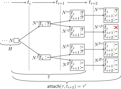
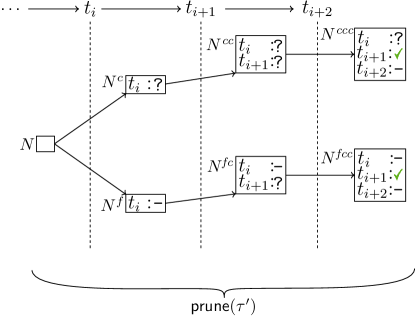
(a)	(b)

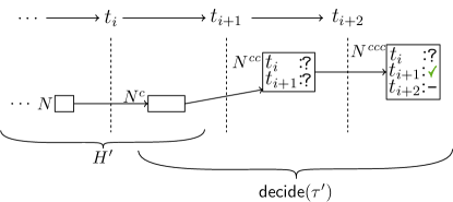
(c)

Figure 6: Application of function $\<step>$ in a blockchain run.

Example 2

Fig. 6 shows the result of applying function $\<step>$ to blockchain run $(H,\tau)$ with a monitoring window $k=2$ and two pending transactions $t_{i}$ and $t_{i+1}$. Each node in the monitoring tree is annotated with the monitor state of all pending transactions up to that node: a question mark means undecided monitors, a tick means known to commit monitors, a cross means known to fail monitors, and a dash denotes no monitored transactions. Initially, no monitors are decided in any node in $\tau$.

Function $\<step>((H,\tau),t_{i+2})$ first invokes function $\<extend>(\tau,t_{i+2})$. This function adds a new level to $\tau$ by applying transaction $t_{i+2}$ at all leaves in $\tau$, obtaining monitoring tree $\tau^{\prime}$, Fig. 6(a). Transaction $t_{i+2}$ immediately commits at all leaves in $\tau$, generating nodes $N^{\textit{ccc}},N^{\textit{cfc}},N^{\textit{fcc}}$ and $N^{\textit{ffc}}$. The future monitor for transaction $t_{i}$ is known to fail at node $N^{\textit{cfc}}$ while remaining undecided at node $N^{\textit{ccc}}$ and the future monitor for transaction $t_{i+1}$ is known to commit at nodes $N^{\textit{ccc}}$ and $N^{\textit{fcc}}$. Next, as the height of the new monitoring tree, $\tau^{\prime}$, is $3>2$, function $\<step>$ invokes function $\<prune>(\tau^{\prime})$ to decide if the first pending transaction, $t_{i}$, fails or commits. Function $\<prune>$ invokes function $\<innerprune>$ to remove all impossible nodes in $\tau^{\prime}$. When computing $\<innerprune>$, the failing subtree of node $N^{c}$, rooted at node $N^{\textit{cf}}$, is removed because at node $N^{\textit{ccc}}$ the future monitor for the transaction at node $N^{c}$, $t_{i+1}$, is known to commit and node $N^{\textit{ccc}}$ is the only future in the committing subtree of node $N^{c}$, making the subtree rooted at $N^{\textit{cf}}$ an impossible subtree. Similarly, the subtree rooted at $N^{\textit{ff}}$ is an impossible subtree and it is also removed by function $\<innerprune>$.

Subtrees with roots $N^{\textit{cf}}$ and $N^{\textit{ff}}$ are the only ones removed when applying function $\<innerprune>$ to monitoring tree $\tau^{\prime}$, as shown in Fig. 6(b).

Finally, to decide whether to commit or not transaction $t_{i}$ function $\<prune>$ consider node $N^{\textit{ccc}}$, as it is the only future in the committing subtree of node $N$ in the monitoring tree returned by function $\<innerprune>$. At node $N^{\textit{ccc}}$ the future monitor for transaction $t_{i}$ is undecided. However, since its monitoring window has ended, function $\<prune>$ uses the $\<timeout>$ of the contracts that are undecided. Assuming for all undecided contracts their $\<timeout>$ function commit transaction $t_{i}$, then function $\<prune>$ commits transaction $t_{i}$, returning the subtree rooted at $N^{c}$ as the new monitoring tree (see Fig. 6(c)), it would fail if at least one contract timeout function fails. Finally, function $\<step>$ extends $H$ by making transaction $t_{i}$ permanent. If $\<innerprune>$ had not been applied before function $\<prune>$ evaluated all futures in the committing subtree of $N$, transaction $t_{i}$ would have incorrectly failed, as in impossible future $N^{cfc}$, the future monitor for transaction $t_{i}$ fails.

Appendix 0.A shows an example of contracts that only lend their tokens if they receive them back within $2$ transactions in the future.

4 Properties

We discuss now properties of the model of computation defined in Section 3. In particular, we establish how the new model extends the previous one, that the size of monitoring trees is manageable, and the blockchain always progresses. We assume a fixed monitoring window $k$. All proofs can be found in Appendix 0.B.

After the monitoring window has expired, the root transaction is confirmed and one of two possible successors is consolidated. monitoring-tree Let $(H,\tau)$ be the system run after $k$ transactions, $t$ a transaction and $(H^{\prime},\tau^{\prime})=\<step>((H,\tau),t)$. The root of $\tau^{\prime}$ is one of the successors of the root of $\tau$ and all paths in $\tau^{\prime}$ without leaves are also paths in $\tau$. Moreover, $H^{\prime}$ is obtained by extending $H$ with the first pending transaction on $\tau$.

The first $k$ transactions from the genesis are just added to the tree. From the previous lemma, after $k$ transactions and when a new step is taken, the first pending transaction is either committed or failed and a new pending transaction is attached to all leaves. Moreover, the transaction added to the history is the root of the previous monitoring tree and one of its successors is the root of the new monitoring tree. In other words, exactly one of the paths in the monitoring tree eventually becomes permanent, and thus, the blockchain always progresses.

Corollary 1 (Progress)

Function $\<step>$ is total and, after the first $k$ invocations, each execution of $\<step>$ makes one transaction permanent.

The height of the monitoring tree is bounded by the monitoring window.

bounded-certainty[Bounded Certainty] Let $\tau$ be a monitoring tree in a blockchain run obtained by applying function step $l$ times. Then, the height of $\tau$ is the minimum between $l$ and $k$. Moreover, all leaves in $\tau$ are in its last level.

Function $\<innerprune>$ removes all impossible nodes from monitoring trees. Function $\<innerprune>$ recursively removes impossible nodes in the committing and failing subtrees, and then, determines if it can remove any subtree by inspecting all possible futures in the committing successor. innerprune-subtree Function $\<innerprune>(\tau)$ returns a sub-monitoring tree of $\tau$ without impossible nodes and only impossible nodes were removed.

Function $\<step>$ consistently makes the blockchain progress. After more than $k$ transactions were added, the first pending transaction is made permanent (see Corollary 1). The resulting monitoring tree keeps the order of the rest of the pending transactions and it also preserves the same information of the pending transactions except the last.

prune Let $\tau$ be a monitoring tree, $\eta$ be the result of expanding $\tau$ with a new transaction, $t$ be the first pending transaction in $\tau$, and $\nu$ be the decided subtree of $\eta$.

• If $\eta$ has only one successor then $\nu$ is the result of pruning $\eta$’s successor.

• If $\eta$ has two successors, then let $\eta_{c}$ and $\eta_{f}$ be the result of pruning the committing and failing subtrees of $\eta$ respectively.

  • Monitoring tree $\nu$ is $\eta_{c}$ if in all possible futures assuming $t$ commits, transaction $t$ does not fail or if no decision has been reached, all pending $\<timeout>$ functions of $t$ commit.

  • Monitoring tree $\nu$ is $\eta_{f}$ if there is a possible future where assuming transactions $t$ commits, leads to the monitor of $t$ fail or some of the pending $\<timeout>$ function of $t$ fail.

The size of monitoring trees can be exponential in the number of monitored transaction rather than in the monitoring window size, as monitored transactions are the only ones branching monitoring trees. size Let $\tau$ be a monitoring tree and $m$ be the number of monitored transactions in $\tau$ (so $m\leq k$). Then, the size of $\tau$ is in $\mathcal{O}(2^{m}\times k)$.

In practical scenarios, the number of monitored transactions typically is small compared to the monitoring window because most transactions do not require future monitors. This makes the size of the monitoring tree much smaller than the theoretical maximum.

Corollary 2

If the number of monitored transactions in monitoring trees is constant then the size of monitoring trees is bounded by $\mathcal{O}(k)$.

Finally, we show that adding future bounded monitors preserves legacy executions, so for blockchain runs where no contracts use future monitors, the monitoring tree is a chain with no branching.

A legacy monitoring tree $\tau$ is such that every configuration obtained from applying $\<applytx>$ coincides with rule $\leadsto$.

legacy-tx[Legacy Pending Transactions]  Let $\tau$ be a legacy monitoring tree. Then, $\tau$ is a chain and the effect of executing all transactions in $\tau$ is equivalent to executing them in the traditional model of computation.

If we add that the permanent history is equivalent (up to now) to the traditional model, then the evolution of the blockchain in both models coincide.

legacy[Legacy History]  Let $\tau$ be a legacy monitoring tree and $H$ be a history such that every permanent transaction coincides with rule $\leadsto$. Then, the result of concatenating $H$ and $\tau$ is equivalent to the traditional model of computation.

From Corollary 1 and Lemma 2, we conclude that the new model of computation is consistent with the previous model of computation and eventually creates a chain. Additionally, Corollary 2 implies that in practical scenarios, the size of monitoring trees is linear on the monitoring window, making it a feasible and practical blockchain implementation.

5 Atomic Loans

Flash loan contracts allow other contracts to borrow tokens without any collateral only if the borrowed tokens are repaid during the same transaction [11] (typically with some interest). Atomic loans are a generalization of flash loans where the borrowing party can repay the lending party in future transactions. It is not possible to implement flash loans unless additional mechanisms are added to the blockchain [10]. Similarly, it is impossible to implement atomic loans in traditional blockchain computational models. As transaction monitors [10] enable flash loans transactions, future monitors allow monitors to check properties across transactions enabling atomic loans. We illustrate now how to implement atomic loans using the monitoring window as the maximum payback time.

We specify lender contracts as contracts respecting the following two properties:

Specification 1 (Atomic Loans)

We say contract $\mathsf{A}$ is an atomic lender if:

AL-safety:

A loan from $\mathsf{A}$ is repaid to $\mathsf{A}$ within the monitoring window.

AL-progress:

Contract $\mathsf{A}$ grants loans unless AL-safety is violated.

The following contract FlashLoanLender shows a simple contract implementing a flash loan lender using Fail/NoFail hookup [10], i.e. with no future monitors but transaction monitors. We highlight monitor code with gray background.

Function lend lends as long as the lender has enough funds, annotates the borrowed tokens in pending_returns and sets its fail bit so the transaction commits only if the loan is paid back. When the loan is returned, returnLoan decreases pending_returns and updates its fail bit. At the end of each transaction, if there are pending loans the fail bit will make the transaction fail.

The above contract implements flash loans that must be returned within a transaction, but does not work properly if future transactions are considered. It is not possible to successfully predict or check whether the loan is returned in some future transactions. We show now how future monitors solve this problem.

The following contract Lender is an atomic lender using future monitors. All loans are treated equally and should be paid back on time, and if one loan is not returned, then all loans issued at the same transaction would be rejected. Here we are being too strict compared to practical cases, but it is enough to illustrate the use of future transaction monitors.

Contract Lender uses a map pending_returns, from transactions to the amount borrowed within that transaction, to determine whether a transaction should commit or fail. Function lend grants a loan if the lender has enough funds, increases the corresponding entry in map pending_returns for the current transaction and sets the failmap entry activating the current transaction monitor. Client contracts can repay loans by invoking returnLoan, which receives the transaction identifier of the lending transaction to decrease the corresponding entry in pending_returns by the amount received. If pending_returns reaches 0 for a given transaction, the failmap entry of that transaction is set to COMMIT. Finally, timeout returns FAIL to fail transactions with unpaid loans at the end of their monitoring window.

Clients can request loans without further collateral, satisfying AL-progress, and if loans are not returned within the monitoring window, the lending transaction will retroactively fail, satisfying AL-safety.

The following contract NaiveClient requests a loan invoking borrow.

In subsequent transactions, the client can invest the funds, and in a final transaction, return the loan to the lender invoking payBack.

Let NC and L be two contracts installed in a blockchain with a monitoring window of length $2$, where NC runs NaiveClient and L runs Lender. Consider $(\Sigma,\Delta)$ to be the current state of the blockchain at which NC has 100 tokens and L has 1000 tokens. From $(\Sigma,\Delta)$, the sequence of transactions is: (1) NCrequests a loan, (2) NCinvests assuming contract L lends the money, and (3) NCreturns the loan. Because L employs future monitors to guarantee clients pay back, the first transaction generates a branching on the blockchain evolution. The next two transactions are not monitored, thus they do not create any branching. Therefore, after these three transactions, there exist two possible futures as shown in Fig.7, one where L grants the loan and another where it does not.

Figure 7: Balance of contracts NC and L in the monitoring tree after executing the three transactions posted by a client.

We can see that NC pays back in all possible futures. Moreover, contract NC pays back even in the future where contract L fails the past lending operation (for a detailed explanation see Appendix 0.C).

A malicious lender can take advantage of such behavior, for example using the following contract MaliciousLender.

The above malicious lender, upon receiving a loan request in function lend, if it has enough tokens, it grants the loan and marks the transaction as undecided using its failmap map. However, this lender contract does not update its failmap map when receiving paybacks. Therefore, at the end of the monitoring window, the monitor remains undecided making the lending transaction fail due to the timeout function. In other words, the malicious lender never lends any tokens, as all its loans are reverted, but it looks like it does. When combined with NaiveClient and the same three transactions described earlier, the malicious lender will receive the repayment of a loan from client NC without having given the loan. In Fig. 7, the bottom branch is the one that survives when the lender implements a malicious contract.

The problem arises because client NC does not implement any mechanism to check in which branch it is executing when repaying the loan. The naive contract does not distinguish between the scenario where the loan will ultimately be committed and the scenario where it will fail. As a result, client NC ends up providing payments in both cases.

The following contract Client presents a correct client implementing a map, toPay, to keep track of its debts to lenders.

The above contract allows clients to determine the specific path in which it is executing, and thus, to decide whether to repay. Consequently, clients can successfully get loans from correct lenders while being resistant to attacks from malicious lenders.

Fig. 8 shows an execution following the same transactions as before but with the correct contract Client: clients request a loan, invest the money, and payback the loan. The top branch shows the case where the lender sends the money and the client returns it, while the bottom branch shows the case where the loan is not given. In the former cases, the client returns the money, and in the latter case, the client just fails the transaction.

Figure 8: Balance of contracts C and L in the monitoring tree after executing the three transactions posted by a client.

These examples show how even contracts not monitoring transactions need to be aware that transactions can create potential executions in the blockchain evolution that may be reverted due to future monitors. Since the same transaction is executed in all possible scenarios, but their effects may be different, contracts need to know in which temporal line they are executing and act accordingly. Contract Client accomplishes this by maintaining a record of debts owed to lenders in variable toPay.

6 Related Work

Dynamic verification of smart contracts

Runtime monitoring tools like ContractLarva [14, 6] and Solythesis [17] take a smart contract code and its properties as input and produce a safe smart contract that fail transactions violating the given properties. They achieve this be injecting the monitor into the smart contract as additional instructions. Therefore, these monitors are restricted to one operation in a single contract. Transaction Monitors [10] extend monitoring beyond a single operation to observe the effect of an entire transaction execution on a given contract.

While these existing works provide strong foundations for smart contract verification, none directly address the ability to react based on future transactions, as proposed in this work.

Branching Computational Models

The monitoring tree generated by pending transactions might reassemble the tree-like structure in branching-time logic such as CTL [12]. However, it is worth noting that the branching in the monitoring tree represent all possible futures given by the monitors of the pending transaction, and exactly one path eventually consolidates. More important, future monitors are not aware of the existence of the other paths in the monitoring tree and therefore cannot reason about them. CTL, on the other hand, can be used to express properties that reason about the different paths in the tree.

7 Conclusion

We presented future monitors for smart contracts. Future monitors are a defense mechanism enabling contracts to state properties across multiple transactions. These kinds of properties are motivated by long-lived transactions, in particular by atomic loans, which are not implementable in their full generality in current blockchains. To implement future monitors, we introduced the notion of monitoring window and two additional new mechanisms to blockchains, namely failing maps and timeout functions.

Future monitors delay the consolidation of transactions, but the system remains consistent and we gain in expressivity. The outcome of transactions remains deterministic and depends solely on the transactions themselves, but now transactions can fail because of future actions. Combining all elements we obtained a deterministic semantics with future monitors in place.

We have also illustrated that contracts need to be aware of the existence of possible executions. Future monitors introduce a branching model to describe the evolution of blockchain systems where transactions may commit or not, caused by the temporary uncertainty regarding the effect of pending transactions. Consequently, when new transactions are added to the blockchain, they are executed in multiple blockchain configurations, representing possible time-lines. Therefore, contracts need to be aware of the different contexts in which they are executing, ensuring that the transaction produces the desired effects in all possible realities.

The main contribution of this paper is theoretical and we left the full implementation of future monitors as future work. Optimistic rollup systems, where the effect of transactions is already delayed due to the fraud-prove arbitration scheme, present an ideal environment to incorporate future monitors into practical blockchain systems without further implications. In particular, optimistic rollup systems can allow future transaction monitors with little modifications, and more importantly, without modifying the underlying blockchain.

For simplicity, we have neglected a specific analysis of the additional gas consumption that arises for using future monitors, which might lead to the failure of accepting transactions. Nevertheless, we conjecture that future monitors are simple enough to guarantee that a calculable amount of gas will prevent gas failing situations. However, we leave a detailed study for future work.

Appendix 0.A Two-bounded Monitor Example

In this section we show an example of the evolution of the system proposed in Section 3.3. The example consists of three contracts exchanging two tokens between them in a blockchain accepting a monitoring window of length $2$.

Let $a,b,c$ be three contracts installed in the blockchain such that both $a$ and $b$ have one token each. Contracts $a$ and $b$ use future monitors and only send their tokens if they will receive their (respective) token back within 2 transactions. For simplicity, in this example, we neglect gas consumption.

Let $(\Sigma_{0},\Delta_{0})$ be a blockchain configuration such that contracts $a,b,c$ are installed and $a$ and $b$ have a token each while $c$ has none. In Fig. 9, we show the evolution of the system beginning from configuration $(\Sigma_{0},\Delta_{0})$ and executing the following three transactions in order: (1) transaction $t_{a,c}$, smart contract $a$ sends its token to $c$; (2) transaction $t_{b,c}$, smart contract $b$ sends its token to $c$; (3) transaction $t_{c,\langle a,b\rangle}$, smart contract $c$ sends tokens to $a$ and $b$. The transaction $t_{c,\langle a,b\rangle}$ involves several internal operations where $c$ sends a token to $a$ and $b$. In Fig. 9(a), we show the initial blockchain run $(H_{0},\tau_{0})$ where both $H_{0}$ and $\tau_{0}$ have a node $N_{0}$ with the initial configuration $(\Sigma_{0},\Delta_{0})$. Let $(H_{1},\tau_{1})$ be the resulting run after contract $a$ sends its token to contract $c$, i.e. executing transaction $t_{a,c}$ (See Fig. 9(b-$\<step>((H_{0},\tau_{0}),t_{a,c})$)). Blockchain run $(H_{1},\tau_{1})$ is the result of executing transaction $t_{a,c}$ to history $H_{0}$ and monitoring tree $\tau_{0}$, in symbols, $\<step>((H_{0},\tau_{0}),t_{a,c})=(H_{1},\tau_{1})$. Internally, function $\<step>$ firsts extends $\tau_{0}$ by executing transaction $t_{a,b}$ in its only leaf, $N_{0}$. Since $a$ only sends its token if it can get it back, the result of executing $t_{a,c}$ in $N_{0}$ depends on future transactions creating a branching in the monitoring tree. In its committing successor, $N^{c}_{1}$, contract $a$ token is sent to $c$, as the transaction is assumed to commit in this scenario. In the failing successor, $N^{f}_{1}$, contract $a$ keeps its token. Since the monitoring tree has height $1<2+1$, the monitor window for the first pending transaction has not expired, and the history remains unchanged, $H_{1}=H_{0}$.

Similar to the first transaction, now we execute the second transaction where contract $b$ sends its token to contract $c$ resulting in another run $(H_{2},\tau_{2})$ (See Fig.9(c-$\<step>((H_{1},\tau_{1}),t_{b,c})$)). First, it extends $\tau_{1}$ by executing transaction $t_{b,c}$ in its leaves, $N^{c}_{1}$ and $N^{f}_{1}$. In both configurations, contract $b$ has a token and only sends it if it can get it back within the monitoring window, and thus, we branch again in both cases generating four possible configurations:

• At configuration $N^{\textit{cc}}_{2}$, the committing successor of $N^{c}_{1}$, contract $c$ has both tokens, as transactions $t_{a,c}$ and $t_{b,c}$ are assumed to commit in this scenario.

• At configuration $N^{\textit{cf}}_{2}$, the failing successor of $N^{c}_{1}$, contract $b$ has its token and contract $c$ has contract $a$ token, as transaction $t_{a,c}$ is assumed to commit while transaction $t_{b,c}$ is assumed to fail.

• At configuration $N^{\textit{fc}}_{2}$, the committing successor of $N^{f}_{1}$, is the dual case of the previous one.

• At configuration $N^{\textit{ff}}_{2}$, the failing successor of $N^{f}_{1}$, contracts $a$ and $b$ have their tokens, as transactions $t_{a,c}$ and transaction $t_{b,c}$ are assumed to fail.

Since the monitoring tree has height $2<2+1$, no decision needs to be made about the first pending transaction, and the history remains unchanged: $H_{2}=H_{1}=H_{0}$.

Finally, we apply the last transaction, $t_{c,\langle a,b\rangle}$, to blockchain run $(H_{2},\tau_{2})$. We show the resulting run in Fig. 9(d-$\<step>((H_{2},\tau_{2}),t_{c,\langle a,b\rangle})$), and since it is the first time a monitoring window ends, we also show the intermediate states in Fig. 9(d-$\<extend>(\tau_{2},t_{a,\langle a,b\rangle})$) and (d-$\<innerprune>(N^{c}_{1})$). We execute transaction $t_{c,\langle a,b\rangle}$ in all four leaves of $\tau_{2}$, resulting in one configuration in all cases, as no contract monitors transaction $t_{c,\langle a,b\rangle}$. There is only one configuration where contract $c$ has enough tokens to perform $t_{c,\langle a,b\rangle}$, $N^{\textit{cc}}_{2}$, and thus, in its committing successor, $N^{\textit{ccc}}_{3}$, tokens are returned to $a$ and $b$. At the other configurations, $N^{\textit{fc}}_{2},N^{\textit{cf}}_{2}$ and $N^{\textit{ff}}_{2}$, transaction $t_{c,\langle a,b\rangle}$ fails, and thus, all the remaining leaves have only a failing successor. The intermediate monitoring tree resulting from attaching transaction $t_{c,\langle a,b\rangle}$ at $\tau_{2}$, $\tau^{\prime}_{2}$, is shown in Fig. 9(d-$\<extend>(\tau_{2},t_{c,\langle a,b\rangle})$).

The monitoring window for transaction $t_{a,c}$ has ended and a decision has to be made. To that end, function $\<step>$ invokes function $\<prune>$ to decide if the first pending transaction, $t_{a,c}$, fails or commits. Function $\<prune>$ first invokes function $\<innerprune>$ to remove all impossible nodes. Function $\<innerprune>$ is recursively applied to all subtrees. Fig. 9(d-$\<innerprune>(N^{c}_{1})$) shows the result of pruning the subtrees with root $N^{c}_{1}$. The future monitor for transaction at $N^{c}_{1}$, $t_{b,c}$, commits if $b$ receives its token back before its monitoring window ends, which happens in $N^{\textit{ccc}}_{3}$, the only future in $N^{c}_{1}$ committing subtree. Therefore, all nodes in the failing subtree of $N^{c}_{1}$ are impossible and hence removed by function $\<innerprune>$. Similarly, the future monitor for transaction at $N_{0}$, $t_{a,c}$, commits if $a$ receives its token back before its monitoring window end, which happens in $N^{\textit{ccc}}_{1}$, the only possible future in $N_{0}$ committing subtree. Hence, all nodes in the failing subtree of $N_{0}$ are impossible and removed by function $\<innerprune>$. Therefore, once the pruning is complete, node $N_{0}$ has no failing successor and its committing subtree is the pruned version of the subtree rooted at $N^{c}_{1}$. Then, function $\<prune>$ returns the pruned subtree at $N^{c}_{1}$ as the new monitoring tree, $\tau_{3}$, committing transaction $t_{a,c}$. Finally, function $\<step>$ extends $H_{2}$ by making transaction $t_{a,c}$ permanent to obtain the new history $H_{3}$ (see Fig. 9(d-$\<step>((H_{2},\tau_{2}),t_{c,\langle a,b\rangle})$)). Notice that if node $N^{\textit{cff}}_{3}$ had been considered when deciding to commit or fail transaction $t_{a,c}$, its future monitor would have incorrectly failed, as $a$ token is not returned in the configuration at node $N^{\textit{cff}}_{3}$, but that node is impossible.

(a)	(b-$\<step>((H_{0},\tau_{0}),t_{a,c})$)	(c-$\<step>((H_{1},\tau_{1}),t_{b,c})$)

(d-$\<extend>(\tau_{2},t_{c,\langle a,b\rangle})$	(d-$\<innerprune>(N^{c}_{1})$)

(d-$\<step>((H_{2},\tau_{2}),t_{c,\langle a,b\rangle})$)

Figure 9: Blockchain system evolution

Appendix 0.B Properties Proofs

In this appendix section, we prove the properties of the model of computation presented in Section 4. We assume there is a fixed monitoring window $k>0$.

The result of pruning a monitor tree is a monitor subtree of the original one where we keep the root.

Lemma 2

Let $\tau$ and $\nu$ be a monitoring tree such that $\<innerprune>(\tau)=\nu$. Then, $\nu$ is a subtree of $\tau$ with the same root as $\tau$ and all leaves in $\nu$ are also leaves in $\tau$.

Proof

The proof is by structural induction on the tree structure of monitor tree $\tau$.

Base Case: If $\tau$ is a leaf, then $\nu=\tau$ and the claim trivially holds.

Inductive Step: We split the inductive step into two cases, based on the number of successors of $\tau$:

• Monitor tree $\tau$ has only one successor $\tau^{\prime}$: By inspecting the definition of $\<innerprune>$, we can see that the result of $\<innerprune>(\tau)$ is a tree that has the same root as $\tau$ and in its only successor is the pruned version of $\tau^{\prime}$, $\nu^{\prime}$. By the inductive hypothesis, all leaves in $\nu^{\prime}$ are also leaves in $\tau^{\prime}$. Since all leaves in $\tau^{\prime}$ are also leaves in $\tau$, it follows that all leaves in $\nu$ are also leaves in $\tau$. Finally, by inductive hypothesis, $\nu^{\prime}$ is a subtree of $\tau^{\prime}$ with the same root as $\tau^{\prime}$, making $\nu$ a subtree of $\tau$.

• If $\tau$ has two successors, then there are three cases depending on if function $\<innerprune>$ removes the failing subtree of $\tau$, the committing subtree of $\tau$ or neither. For all three cases, the proof is analogous to the previous case.

Now, we prove each lemma stated in Section 4.

Lemma LABEL:bounded-certainty

Proof

The proof is by induction on the number of steps taken by the step function, $l$:

Base Case: If no transaction were added, $l=0$, then $\tau$ contains only one node, the initial configuration, and the lemma follows.

Inductive step: Let $(H^{\prime},\nu)$ be a blockchain run obtained by applying function $\<step>$ $l$ times, and $t$ a transaction such that $\<step>((H^{\prime},\nu),t)=(H,\tau)$. Function $\<step>$ starts by invoking function $\<extend>(\nu,t)$, which returns a new monitoring tree, $\eta$, obtained by adding one or two successors to each leaf in $\nu$. Then, all leaves in $\eta$ are added nodes. By inductive hypothesis, all leaves in $\nu$ are in its last level. Then, all leaves in $\eta$ are also its last level.

Furthermore, by inductive hypothesis, the height of $\nu$ is $\min(k,l)$, hence the height of $\eta$ is $\min(k,l)+1$. If $l<k$ then $\tau=\eta$ and the lemma follows. Otherwise, the height of $\eta$ is $k+1$ and function $\<step>$ invokes function $\<prune>$, setting $\tau=\<prune>(\eta)$. Function $\<prune>$ returns a subtree rooted in one of the successors of $\<innerprune>(\eta)$, thus the height of $\tau$ is one less than the height of the pruned version of $\eta$. Lemma 2 directly implies that $\<innerprune>(\eta)$ has the same height as $\eta$. As consequence, the height of $\tau$ is $(k+1)-1=k$.

Lemma LABEL:monitoring-tree

Proof

Function $\<step>((H,\tau),t)$ begins by invoking function $\<extend>(\tau,t)$ which returns a new monitoring tree, $\nu$, obtained by adding one or two successor to each leaf in $\tau$. Thus, the height of $\nu$ is one more than the height of $\tau$. By lemma 1, the height of $\tau$ is $k$, so the height of $\nu$ is $k+1$. Therefore, function $\<step>$ extends history $H$ by making permanent the first transaction in $\tau$ to obtain $H^{\prime}$, and invokes function $\<prune>$ to get the new monitoring tree, that is, $\tau^{\prime}=\<prune>(\nu)$. Function $\<prune>(\nu)$ first invokes function $\<innerprune>(\nu)$, to obtain the pruned version of $\nu$, $\eta$, and then functions $\<prune>$ returns either the committing or failing subtree of $\eta$. That is, $\tau^{\prime}$ is either the committing or failing subtree of the pruned version of $\nu$. Since $\eta$ is a subtree of $\nu$ with the same root as $\nu$ (see Lemma 2), the root of $\tau^{\prime}$ is one of the successors of the root of $\nu$, which, by definition of $\nu$ is one of the successors of the root of $\tau$. Finally, from Lemma 2, all paths in $\tau^{\prime}$ are also path in $\nu$. Specifically, all paths without leaves in $\tau^{\prime}$ are also path without leaves in $\nu$. And, by definition of $\nu$, all paths without leaves in $\nu$ are path in $\tau$. Consequently, all paths without leaves in $\tau^{\prime}$ are path in $\tau$.

Lemma LABEL:innerprune-subtree

Proof

The proof is by induction in $\tau$.

Base Case: If $\tau$ is a leaf, then it is not impossible and $\<innerprune>(\tau)=\tau$.

Inductive Step: There are two cases, depending on the number of successors of $\tau$:

• if $\tau$ has only one successor, $\eta$, then $\<innerprune>(\tau)$ returns a tree, $\tau^{\prime}$ that has the same root as $\tau$ and in its only successor is the pruned version of $\eta$, $\eta^{\prime}$. By inductive hypothesis, $\eta^{\prime}$ does not have impossible nodes; thus, $\tau^{\prime}$ does not have impossible nodes either. Moreover, only the nodes removed when pruning $\eta$ are removed from $\tau$, and by inductive hypothesis, those nodes are impossible. Consequently, only impossible nodes are removed from $\tau$.

• if $\tau$ has two successors, $\eta_{c}$ and $\eta_{f}$, $\<innerprune>$ computes the pruned version of each of them, $\eta^{\prime}_{c}$ and $\eta^{\prime}_{f}$, respectively. By inductive hypothesis, $\eta^{\prime}_{c}$ has no impossible nodes, thus, by inspecting the status of the future monitor of the transaction at the root of $\tau$ in all leaves in $\eta^{\prime}_{c}$ one can know if there are impossible nodes in $\tau$. If in all futures in $\eta^{\prime}_{c}$ the future monitor is known to commit, then all nodes in the failing subtree of $\tau$ are impossible. In this case, function $\<innerprune>$ returns a tree that has the same root as $\tau$ and its only successor is $\eta^{\prime}_{c}$. Similarly, if in all futures in $\eta^{\prime}_{c}$ the future monitor is known to fail, then all nodes in the committing subtree of $\tau$ are impossible, and function $\<innerprune>$ returns a tree that has the same root as $\tau$ and in its only successor is $\eta^{\prime}_{f}$. Otherwise, function $\<innerprune>$ returns a tree that has the same root as $\tau$ and in its successors are $\eta^{\prime}_{c}$ and $\eta^{\prime}_{f}$. In all cases, the lemma follows by inductive hypothesis.

Lemma LABEL:prune

Proof

It follows directly from Lemma 1, which ensures that the pruned version of monitoring trees do not contain impossible nodes, and the definition of function $\<prune>$ (see Fig. 5).

Lemma LABEL:size

Proof

By lemma 1 monitoring trees have height at most $k$. For this proof we consider, w.l.o.g., monitoring trees with height exactly $k$.

By construction, nodes in monitoring trees have at most two successors. New successors are only added inside function $\<extend>$. Specifically, $\<extend>$ adds two successors to a node only if the corresponding transaction is being monitored. Thus, the $m$ levels in the monitoring tree that correspond to monitored transactions can have at most double the number of nodes of the previous level. On the other hand, the $k-m$ levels in the monitoring tree that correspond to unmonitored transactions have the same number of nodes as the previous level. Therefore, a monitoring tree has the maximal number nodes when monitored transactions generate branching in all nodes that are applied, and they precede all unmonitored transactions. In this case, the first $m$ levels of the monitoring tree correspond to a complete binary tree, and the remaining $k-m$ levels have the same number of nodes as the last level of that complete binary tree, which is $2^{m}$. Consequently, the maximal size of monitoring trees with $m$ monitored transactions is $2^{m+1}-1+2^{m}\times(k-m)$ which is in $\mathcal{O}(2^{m}\times k)$.

Lemma LABEL:legacy-tx

Proof

Let $n$ be a node in $\tau$ that is not a leaf, such that its extended blockchain configuration is $(\Sigma,\Delta,\mathcal{U})$ and $\<nextTx>(n)=t$. Then, since $\tau$ is a legacy monitoring tree, the function $\<applytx>$ can return two possible values:

• Transaction commits, $\<applytx>(n,\<nextTx>(n))=\mathbf{Commit}(\Sigma_{c},\Delta_{c},\mathcal{U}_{c})$, producing a committing step $(\Sigma,\mathcal{U})\leadsto_{t}(\Sigma_{c},\mathcal{U}_{c})$. As $\<extend>$ is the only function that adds edges to monitoring trees, it follows that $n$ has only one successor, whose extended blockchain configuration is $(\Sigma_{c},\Delta_{c},\mathcal{U}_{c})$.

• Transaction fails, $\<applytx>(n,\<nextTx>(n))=\mathbf{Fail}(\Sigma,\Delta,\mathcal{U}_{f})$, producing a failing step $(\Sigma,\mathcal{U})\leadsto_{t}(\Sigma,\mathcal{U}_{f})$. Similarly, in this case, node $n$ also has only one successor, whose extended blockchain configuration is $(\Sigma,\Delta,\mathcal{U}_{f})$.

In consequence, monitoring tree $\tau$ is a chain, and for each pair of consecutive nodes $n_{i}\xrightarrow{\<tx>}n_{i+1}$ with extended blockchain configurations $(\Sigma_{i},\Delta_{i},\mathcal{U}_{i})$ and $(\Sigma_{i+1},\Delta_{i+1},\mathcal{U}_{i+1})$, respectively, the relation $(\Sigma_{i},\mathcal{U}_{i})\leadsto_{tx}(\Sigma_{i+1},\mathcal{U}_{i+1})$ holds. This implies that the execution of transactions in $\tau$ is equivalent to executing them in the traditional model of computation.

Lemma LABEL:legacy

Proof

It follows from that every transaction in $H$ coincides with rule $\leadsto$, the root configuration at $\tau$ being the last configuration in $H$ and Lemma 2.

Appendix 0.C Atomic Loan - Example Explained

In this section, we describe in detail the blockchain evolution of the example presented in Section 5. For simplicity, we neglect gas consumption.

Let NC and L be two contracts installed in a blockchain with monitoring window of length $2$, where NC runs NaiveClient and L runs Lender. Consider $(\Sigma_{0},\Delta_{0})$ to be a blockchain configuration where NC has 100 tokens and L has 1000 tokens. We describe the evolution of the system from blockchain run $(H_{0},\tau_{0})$ with $H_{0}=\tau_{0}=(\Sigma_{0},\Delta_{0})$, and executing the following three transactions in order: (1) $t_{req}$, NC requests a loan for 100 to L; (2) $t_{inv}$, NC invests if it has more than 200 tokens; (3) $t_{ret}$, NC returns the loan to L.

Let $N_{0}$ be the root of $\tau_{0}$. The execution of transaction $t_{req}$ in blockchain run $(H_{0},\tau_{0})$ starts by executing transaction $t_{req}$ in the only leaf of $\tau_{0}$, $N_{0}$. Transaction $t_{req}$ is originated by an external invocation to function borrow.

Within the execution of $t_{req}$, function loan is invoked. Since lender L has enough tokens, it will send the requested amount to client NC, and it will update its pending_returns with the lent amount, and also set the entry for transaction $t_{req}$ to undecided in its failmap map. As consequence, there is a branching in the monitoring tree. In node $N_{0}$’s committing successor, $N^{c}_{1}$, the loan is assumed to take place and the balance of client NC is increased by 100 tokens while the balance of lender L is decreased by 100 tokens. On the other hand, in the failing successor, $N^{f}_{1}$, transaction $t_{req}$ fails and $N^{f}_{1}$ has the same configuration as $N_{0}$ There is no need to prune the new monitoring tree as its height is $1<k+1$, and thus the history remains the same.

In the subsequent transaction, $t_{inv}$, client NC try to invest its tokens by invoking function invest. Transaction $t_{inv}$ executes in both leaves of the monitoring tree, $N_{1}^{c}$ and $N_{1}^{f}$, and since it is not monitored, each of them has one successor. In configuration $N_{1}^{c}$, client NC has enough tokens to invest, resulting in a committing successor, $N_{2}^{\textit{cc}}$, where client NC generated some profit. In configuration $N_{1}^{f}$, client NC does not have enough tokens to invest and therefore, it has only a failing successor, $N_{2}^{\textit{ff}}$, whose blockchain configuration coincides with $N_{1}^{f}$. Again, there is no need to prune the new monitoring tree as its height is $2<k+1$.

Finally, the third transaction, $t_{ret}$, is originated by an invocation to function payBack in client NC, to pay back the 100 tokens loan from transaction $t_{req}$. Transaction $t_{req}$ is executed in configurations at $N_{2}^{\textit{cc}}$ and $N_{2}^{\textit{ff}}$, the leaves of the new monitoring tree. When executing transaction $t_{ret}$ in configuration $N^{\textit{cc}}$, client NC has enough tokens to send to lender L, hence function returnLoan in lender L is invoked with the identifier of transaction $t_{req}$ as parameter. Lender L receives the 100 tokens that it had lent in transaction $t_{req}$, thus it sets the entry corresponding to $t_{ret}$ in its failmap map as COMMIT. Transaction $t_{ret}$ is not monitored and thus $N_{2}^{\textit{cc}}$ has only one committing successor, $N_{3}^{\textit{ccc}}$, where the balance of NC is decreased by 100 tokens and the one of L is increased by 100. Similarly, when executing transaction $t_{ret}$ in configuration $N^{\textit{ff}}$, client NC has enough tokens to send to lender L and function returnLoan in lender L is also invoked with the identifier of transaction $t_{req}$ as parameter. In this case, lender L accepts the 100 tokens, but it does not update its failing map because in this scenario transaction $t_{req}$ have failed, and thus, the value of pending return for transaction $t_{req}$ is set to $-100\neq 0$ during the execution of $t_{ret}$. Transaction $t_{ret}$ is not monitored and thus $N_{2}^{\textit{ff}}$ has only one committing successor, $N_{3}^{\textit{ffc}}$. As transaction $t_{ret}$ is committed in this case, the balance of NC decreases by 100 tokens and the one of L increase by 100, even though L has not lent any tokens to NC in this scenario.

Let $\nu$ be the monitoring tree up until this point. Fig. 7 show the balance of smart contract NC and L in the monitoring tree $\nu$. Monitoring tree $\nu$ has height $3=k+1$, and thus the monitoring window for the first transaction has ended, and a decision to commit or fail it must be taken. The first pending transaction in $\nu$ is $t_{req}$, where client NC requested the loan to lender L. The only leaf in $\nu$ that assumes that transaction $t_{ret}$ has committed is $N_{3}^{\textit{ccc}}$, and in this leaf $t_{ret}$ is committed by the monitor. Consequently, $t_{req}$ is committed, and the subtree with root as the committing successor of $N_{0}$, $N_{1}^{c}$, becomes the new monitoring tree, discarding the failing subtree of $N_{0}$, rooted at $N^{f}_{1}$, that assumes that transaction $t_{req}$ failed.

Even though in this run the configuration $N_{3}^{\textit{ffc}}$ is removed, in that configuration, client NC is paying back a loan to lender L that did not happen.

References

- [1] Michelson: the language of smart contracts in Tezos. https://tezos.gitlab.io/whitedoc/michelson.html.
- [2] Ethereum. Solidity documentation –- release 0.2.0. http://solidity.readthedocs.io/, 2016.
- [3] W. Ahrendt and R. Bubel. Functional verification of smart contracts via strong data integrity. In Proc. of ISoLA (3), LNCS, pages 9–24. Springer, 2020.
- [4] G. Alfour. LIGO: a friendly smart-contract language for Tezos. https://ligolang.org, 2020. last accessed: 2022-05-03.
- [5] D. Annenkov, J. B. Nielsen, and B. Spitters. ConCert: a smart contract certification framework in Coq. In Proc. of the 9th ACM SIGPLAN Int’l Conf. on Certified Programs and Proofs (CPP’20), pages 215–218. ACM, 2020.
- [6] S. Azzopardi, J. Ellul, and G. J. Pace. Monitoring smart contracts: ContractLarva and open challenges beyond. In Proc. of the 18th International Conference on Runtime Verification (RV’18), volume 11237 of LNCS, pages 113–137. Springer, 2018.
- [7] B. Bernardo, R. Cauderlier, Z. Hu, B. Pesin, and J. Tesson. Mi-Cho-Coq, a framework for certifying Tezos smart contracts. arXiv, abs/1909.08671, 2019.
- [8] K. Bhargavan, A. Delignat-Lavaud, C. Fourneta, A. Gollamudi, G. Gonthier, N. Kobeissi, N. Kulatova, A. Rastogi, T. Sibut-Pinote, N. Swamy, and S. Z. Béguelin. Formal verification of smart contracts: Short paper. In Proc. of Workshop on Programming Languages and Analysis for Security (PLAS@CCS’16), pages 91–96. ACM, 2016.
- [9] L. Bousfield, R. Bousfield, C. Buckland, B. Burgess, J. Colvin, E. Felten, S. Goldfeder, D. Goldman, B. Huddleston, H. Kalonder, F. Lacs, H. Ng, A. Sanghi, T. Wilson, V. Yermakova, and T. Zidenberg. Arbitrum nitro: A second-generation optimistic rollup. https://github.com/OffchainLabs/nitro/blob/master/docs/Nitro-whitepaper.pdf, 2022.
- [10] M. Capretto, M. Ceresa, and C. Sánchez. Transaction monitoring of smart contracts. In T. Dang and V. Stolz, editors, Runtime Verification - 22nd International Conference, RV 2022, Tbilisi, Georgia, September 28-30, 2022, Proceedings, volume 13498 of Lecture Notes in Computer Science, pages 162–180. Springer, 2022.
- [11] A. C. Cañada, F. Kobayashi, fubuloubu, and A. Williams. Eip-3156: Flash loans. https://eips.ethereum.org/EIPS/eip-3156.
- [12] E. M. Clarke and E. A. Emerson. Design and synthesis of synchronization skeletons using branching time temporal logic. In D. Kozen, editor, Logics of Programs, pages 52–71, Berlin, Heidelberg, 1982. Springer Berlin Heidelberg.
- [13] S. Conchon, A. Korneva, and F. Zaïdi. Verifying smart contracts with Cubicle. In Proc. of the 1st Workshop on Formal Methods for Blockchains (FMBC’19), volume 12232 of LNCS, pages 312–324. Springer, 2019.
- [14] J. Ellul and G. J. Pace. Runtime verification of Ethereum smart contracts. In Proc. of the 14th European Dependable Computing Conference (EDCC’18), pages 158–163. IEEE Computer Society, 2018.
- [15] J. Ellul and G. J. Pace. Optional monitoring for long-lived transactions. In W. Ahrendt, D. Ancona, and A. Francalanza, editors, VORTEX 2021: Proceedings of the 5th ACM International Workshop on Verification and mOnitoring at Runtime EXecution, Virtual Event, Denmark, 12 July 2021, pages 35–39. ACM, 2021.
- [16] J. Gray. The Transaction Concept: Virtues and Limitations, page 140–150. Morgan Kaufmann Publishers Inc., San Francisco, CA, USA, 1988.
- [17] A. Li, J. A. Choi, and an. Long. Securing smart contract with runtime validation. In Proc. of ACM PLDI’20, pages 438–453. ACM, 2020.
- [18] S. Nakamoto. Bitcoin: a peer-to-peer electronic cash system, 2009.
- [19] Z. Nehaï and F. Bobot. Deductive proof of industrial smart contracts using Why3. In Proc. of the 1st Workshop on Formal Methods for Blockchains (FMBC’19), volume 12232 of LNCS, pages 299–311. Springer, 2019.
- [20] A. Permenev, D. Dimitrov, P. Tsankov, D. Drachsler-Cohen, and M. Vechev. Verx: Safety verification of smart contracts. In 2020 IEEE Symposium on Security and Privacy (SP), pages 1661–1677, 2020.
- [21] D. Phil. Analysis of the dao exploit. https://hackingdistributed.com/2016/06/18/analysis-of-the-dao-exploit/, 2016.
- [22] J. Schiffl, W. Ahrendt, B. Beckert, and R. Bubel. Formal analysis of smart contracts: Applying the KeY system. In Deductive Software Verification: Future Perspectives - Reflections on the Occasion of 20 Years of KeY, volume 12345 of LNCS, pages 204–218. 2020.
- [23] I. Sergey, A. Kumar, and A. Hobor. Scilla: a smart contract intermediate-level LAnguage. CoRR, abs/1801.00687, 2018.
- [24] J. Stephens, K. Ferles, B. Mariano, S. Lahiri, and I. Dillig. SmartPulse: Automated checking of temporal properties in smart contracts. In Proc. of the 42nd IEEE Symposium on Security and Privacy (S&P’21). IEEE, May 2021.
- [25] N. Szabo. Smart contracts: Building blocks for digital markets. Extropy, 16, 1996.
- [26] G. Wood. Ethereum: A secure decentralised generalised transaction ledger. Ethereum project yellow paper, 151:1–32, 2014.