Probing the Spin-Induced Quadrupole Moment of Massive Black Holes
with the Inspiral of Binary Black Holes

Abstract

One of the most important sources for the space-borne gravitational wave detectors such as TianQin and LISA, is the merger of massivie black hole binaries. Using the inspiral signals, we can probe the properties of the massive black holes, such as the spin-induced multipole moments. By verifying the relation among the mass, spin and quadrupole moment, the no-hair theoreom can be tested. In this work, we analysed the capability on probing the spin-induced quadrupole moment with the inspiral signal of massive black hole binaries using space-borne gravitational wave detectors. Using the Fisher information matrix, we find that the deviation of quadrupole moment can be constrained to the level of $10^{-1}$, and the events with higher mass-ratio will give a better constraint. We also find that the late inspiral part will dominate the result of parameter estimation. The result of Bayesian analysis shows that the capability will be improved by a few times due to the consideration of higher modes. We also calculate the Bayes factor, and the results indicate that the model of black hole and Boson star can be distinguished undoubtedly.

I Introduction

After the first detection of the gravitational wave (GW) from GW150914 Abbott et al. (2016), the LIGO-Virgo-KAGRA (LVK) collaboration have already reported 90 events for the merger of stellar mass compact binaries Abbott et al. (2021a, b); Scientific (2021); Abbott et al. (2019), which includes binary black hole (BBH), binary neutron star (BNS), and neutron star-black hole (NSBH) Abbott et al. (2019); Broekgaarden and Berger (2021). Besides the black holes and neutron stars, some models of exotic objects Johnson-McDaniel et al. (2020) such as quarkstarsHaensel et al. (1986), boson stars Kolb and Tkachev (1993), gravastarsMazur and Mottola (2023), and BHs in modified theory of gravity are also proposed as the alternativesCardoso and Pani (2019). The GWs generated by the bianries constituted of these exotic compact objects will be different from BBH, and thus we can use GW to test the nature of the compact objects.

According to the black hole no-hair theorem Hawking (2005), the classical black holes in general relativity are fully characterised by their masses, spins and charges. However, due to various neutralization mechanisms Blandford and Znajek (1977), it’s widely believed that the astrophysical BHs will have negligible electric charge. So these BHs can be characterised by the Kerr metric, which include only the mass $M$ and the spin $a$ as the parameters. By measuring multiple parameters of a BH, and test if they could give a consistent prediction of $M$ and $a$ according to the general relativity (GR), we can test the no-hair theorem and probe the nature of the compact objects.

Various parametrization methods have been proposed for such tests, which include the tidal deformability Hinderer et al. (2010); Chatziioannou (2020); Raithel et al. (2018); Malik et al. (2018), the horizon absorption effectBernuzzi et al. (2012), the quasi-normal mode spectrum of ringdown Kokkotas and Schmidt (1999); Kelly and Baker (2013); Ota and Chirenti (2020); Baibhav et al. (2018); Shi et al. (2019); Berti et al. (2006, 2007); Dreyer et al. (2004); Detweiler (1980) and the multipole moments Poisson (1998); Kastha et al. (2018). With these parametrization, the BH will perform differently compare to the mimickers.

For a localized object, its gravitational field can be expanded in terms of the multipole moments Hansen (1974); Geroch (1970); Thorne (1980); Compere et al. (2018). For a stationary asymptotically flat solutions of Einstein equation, such as the Kerr black hole, the multipole moments can be expressed by the mass $M$ and spin $a$ as

$$\mathcal{M}_{l}+{\rm i}\mathcal{S}_{l}=M({\rm i}a)^{l}$$ (1)

There come up two sets of multipole moments, the mass moments $\mathcal{M}_{l}$ for even $l$s, and the current moments $\mathcal{S}_{l}$ for odd $l$s. The mass multipole moments for odd orders and the current multipole moments for even orders will vanish due to the equatorial symmetry of Kerr solution. The leading order mass moment $\mathcal{M}_{0}=M$ and current moment $\mathcal{S}_{1}=Ma$ are the mass and spin angular momentum of the Kerr BH, respectively. If we can measure the multipole moments with $l\geq 2$ besides the mass and spin, then we can test if these expression is broken, and thus test the no-hair theoreom.

In most of the cases, only the $l=2$ term, which is known as the spin induced quadrupole moment (SIQM), is considered in the relevant test. For a general compact object, the SIQM can be represented as $Q=-\kappa\chi^{2}{M^{3}}$ where $\chi=a/M$ is the dimensionless spin parameter and $\kappa$ is a coefficient depended on the internal structure of the object related to its equation of state Krishnendu et al. (2017). For BHs, we will have $\kappa=1$ according to (1). For NSs, it’s belived that $\kappa$ can varies between 2-14 Laarakkers and Poisson (1999); Pappas and Apostolatos (2012) due to the multipole deformation happening during the rotation processStein et al. (2014), up to quadratic in spin. For BSs, the range of $\kappa$ is about 10 to 150 Herdeiro and Radu (2014); Baumann et al. (2019). For some other BH mimickers such as gravastars, the value also can be negativeUchikata et al. (2016); Dubeibe et al. (2007). Then by measuring $\kappa$, we can distinguish between the BHs and its mimickersRyan (1997a, b).

Using the low mass events in GWTC-2Narikawa et al. (2021), the data support the model of BBH rather than ECO, and $\kappa$ is constrained to the level of $\mathcal{O}(10^{2})$. Recent work has also analyse the impact of spin precession and higher modes on the measurement of SIQM with ground-based detectors Divyajyoti (2023), some selected GWTC events are also used in the data analysis. The combined Beyesian factor among the GWTC events is calculated, $\rm logBF_{\delta\kappa_{s}\neq 0}^{\rm Kerr}=0.9$ Abbott et al. (2021c) in GWTC-3 and 1.1 in GWTC-2Abbott et al. (2021d). The capability is also analysed for LISA and DECIGO Krishnendu and Yelikar (2020) with the detection of massive black hole binarys, and $\kappa$ is expected to be constrained to the level of $\mathcal{O}(0.1)$. Based on some astrophysical model for the population of MBHB, it’s also argued that 3% of the events can reach these level. Moreover, with the detection of extreme mass-ratio inspirals, TianQinFan et al. (2020); Zi et al. (2021); Liu and Zhang (2020) and LISABarack and Cutler (2004, 2007); Babak et al. (2017) can constrain the SIQM to $10^{-5}$.

TianQin is a space-borne GW dectector Luo et al. (2016); Hu et al. (2017) to be launched in 2035. It comprising three drag-free satellites orbiting the Earth at radius of $10^{5}$ km, and aims to dectect GWs on mHz band. The major objectives Mei et al. (2021) including the merger of MBHBs Wang et al. (2019); Feng et al. (2019), the inspiral of stellar mass BBHs Liu et al. (2020, 2022), the of glactic compact binaries Huang et al. (2020), the EMRIsFan et al. (2020, 2022), and the stochastic GW background Liang et al. (2023, 2022). With the observation of these signals, we can also study the evolution of the universe Zhu et al. (2022a, b); Huang et al. (2023), and the nature of BHs and gravity Shi et al. (2019); Bao et al. (2019); Zi et al. (2021); Sun et al. (2023); Xie et al. (2022); Shi et al. (2023); Lin et al. (2023).

In this work, we carry out a more comprehensive study on how well TianQin can test NHT by probing the SIQM with the insprial signal of MBHBs. We consider the higher $(l,m)$ modes corrections due to the deviation of the SIQM, and use the time delay interferometry (TDI) response to generate the signal. With the fisher information matrix (FIM) analysis, we find that the late inspiral will dominate the accuracy of the constraint, which indicates that we don’t need to consider a full inspiral signal in this analysis. The result also shows that the events with asymmetric mass will have better capability, and higher modes will be important for large mass-ratio events. So we also consider these higher modes in our waveform, and the corresponding modifications. Then we use bilby to do the Bayesian analysis, and the accuracy on the estimation of the parameters agrees with the FIM result. For the injection signal with non-zero $\delta\kappa$, if we do not consider this deviation in the matched waveform, the result will show a significant bias on the estimation of other source parameters. By calculating the Bayes factor, we find that the siginal from BHs and ECOs can be distinguished undoubtedly.

The paper is organized as follows. In Section II, we will give a brief review about the basic methods on the waveform, the response, and the statistics in each subsections respectively. Then, we present our results for TianQin with FIM and Bayesian analysis in Section III Finally, we give a brief summary of conclusion in Section IV. Throughout this work, the geometrized unit system $(G=c=1)$ is used.

II Method

II.1 Waveform

In this work, we use the IMRPhenomXHM García-Quirós et al. (2020) waveform, which is a frequency domain model for the inspiral-merger-ringdown of quasi-circular non-precessing BBH with higher modes. In general, the waveform can be written as

$$h_{BBH}(f)=\sum_{lm}A_{lm}(f)e^{i\Psi_{lm}^{BBH}(f)}.$$ (2)

$A_{lm}(f)$ and $\Psi_{lm}^{BBH}(f)$ are the amplitude and phase for the $lm$ mode, respectively. The index ‘BBH’ means that the corresponding formula is derived for BBHs, and it will change for binaries constitude of ECOs. The SIQM of the progenitors and the remanent will influence the phase evolution of inspiral and the quasi-normal mode spectrum of ringdown respectively. In this work, we will focus on the inspiral part, and thus a cutoff at innermost stable circular orbit (ISCO) will be adopted in the following calculation. Since the spin precession is not considered in the waveform we used, we will assume the aligned or anti-aligned spin for the binaries.

For binaries constitude of ECOs, the waveform for inspiral can be modified as

$$h_{ECO}(f)=\sum_{lm}A_{lm}(f)e^{i\left(\Psi_{lm}^{BBH}(f)+\Psi_{lm}^{SIQM}(f)\right)},$$ (3)

which means that we ignore the modification of the amplitudeArun et al. (2009), since the phase will dominate the accuracy of parameter estimation (PE) for intrinsic parameters. If we neglect the tidal effect, and only consider the leading order correction of SIQM, the phase correction for the leading $22$ mode can be expressed as Narikawa et al. (2021); Krishnendu et al. (2017); Arun et al. (2009); Mishra et al. (2016)

$$\Psi^{SIQM}_{22}(f)=\frac{75}{64}\frac{\delta\kappa_{1}M^{2}_{1}\chi^{2}_{1}+\delta\kappa_{2}M^{2}_{2}\chi^{2}_{2}}{M_{1}M_{2}}(\pi M_{tot}f)^{-\frac{1}{3}}.$$ (4)

$M_{tot}=M_{1}+M_{2}$ is the total mass of the binary system, and $\delta\kappa_{i}=\kappa_{i}-1$ characterised the deviation of the SIQM relative to the BH. It should be noticed that, the mass we used is the red-shifted mass all through this paper. The power index of $-1/3$ means that this leading-order correction appears at 2PN order. We set $\delta\kappa_{1}=\delta\kappa_{2}=\delta\kappa$, and thus ignore the antisymmetric contribution. Obviously, the BBH cases corresponding to $\delta\kappa=0$, and we have neglected the BH-ECO system or binary ECOs with different $\kappa$.

For the correction on the phase of the higher modes, we adopt the relation given in the parameterized post-Einsteinian framework Mezzasoma and Yunes (2022). Since the leading order correction appears at 2PN order, the higher modes correction can be writen as:

$$\psi_{lm}^{SIQM}=\left(\frac{2}{m}\right)^{-4/3}\psi_{22}^{SIQM}.$$ (5)

In our analysis, the modes we considered include the dominant mode (2,2) and subdominant modes (2,1) and (3,3).

II.2 The Response and Noise of TianQin

For space-borne GW detectors, TDI Tinto et al. (2004); Marsat et al. (2021) must be used to suppress the laser phase noise. In this work, we use the 1.0 type channel for $A$, $E$, $T$ to do the data analysis, and the signal is the product of the waveform and the transfer function,

$$h_{\tilde{A},\tilde{E},\tilde{T}}=\sum_{lm}\mathcal{T}^{lm}_{\tilde{A},\tilde{E},\tilde{T}}\tilde{h}_{lm}(f)$$ (6)

For details of the formalism of the transfer function for TianQin, we refer Lyu et al. (2023) In this work, we only adopt the $A$ channel in our calculation.

The power spectral density (PSD) for the noise of TianQin corresponding to the TDI channel can be written as

$$\begin{split}S_{A,E}&=8\sin^{2}\frac{f}{f_{*}}\left[(2+\cos\frac{f}{f_{*}})(2\pi f)^{2}S_{x}\right.\\ &\left.+4\left(1+\cos\frac{f}{f_{*}}+\cos^{2}\frac{f}{f_{*}}\right)\left(1+\frac{0.1\rm{mHz}}{f}\right)\frac{S_{a}}{(2\pi f)^{2}}\right]\end{split}$$ (7)

where $f_{*}=\frac{1}{2\pi{L}}$ is the characteristic frequency of TianQin, and $L=\sqrt{3}\times 10^{8}$m is the arm length. The acceleration noise $S_{a}$ and the position noise $S_{x}$ isLuo et al. (2016)

$$\begin{split}&S_{a}=10^{-30}{\rm m}^{2}\cdot{{\rm s}^{-4}}\cdot{{\rm Hz}^{-1}}\\ &S_{x}=10^{-24}{\rm m}^{2}\cdot{{\rm Hz}^{-1}}\end{split}$$ (8)

II.3 Parameter Estimation

In this study, FIM is used to estimate TianQin’s ability on the measurement of the parameters. By the definition of inner product

$$(g|h)\equiv 2\int_{f_{low}}^{f_{high}}\frac{{g(f)^{*}}h(f)+{h(f)^{*}}g(f)}{S_{n}(f)}df,$$ (9)

the FIM is defined as Cutler and Flanagan (1994)

$$\Gamma_{ij}\equiv\left(\frac{\partial{h}}{\partial\theta_{i}}|\frac{\partial{h}}{\partial\theta_{j}}\right)$$ (10)

$h$ is the responsed signal of the injected waveform, and $\theta_{i}$ is the $i$-th parameter of the source. In our analysis, the parameters are chosen as:

$$\theta=\left\{{\mathcal{M},\eta,D_{L},t_{c},\phi_{c},\psi,\iota,\chi_{1},\chi_{2},\delta\kappa_{s}}\right\}$$ (11)

$\eta=\frac{M_{1}M_{2}}{(M_{1}+M_{2})^{2}}$ is the symmetric mass ratio, $\mathcal{M}=M_{tot}{\eta}^{3/5}$ is the chirp mass, and $D_{L}$ is the luminosity distance. $t_{c}$ and $\phi_{c}$ are the time and phase at coalescence. $\psi$ and $\iota$ are the polarization and inclination angle of the source. $\chi_{1}$ and $\chi_{2}$ are the dimensionless spin parameters for each BHs. For a siginal with large signal-to-noise ratio (SNR), the uncertainty on the parameter estimation is given by

$$\Delta\theta_{i}=\sqrt{\Gamma^{-1}_{ii}}$$

In the calculation of the inner product, the lower and higher frequency bounds are chosen as

$$\begin{split}&f_{high}=min(f_{max},f_{isco})\\ &f_{low}=max(f_{min},f_{init})\end{split}$$ (12)

Due to the sensitivity band of TianQin, we set $f_{max}$=1Hz, $f_{min}$=$10^{-4}$Hz, and the signal beyond this band will be ignored. $f_{init}$ is the initial frequency of the source, and it depends on the time $T$ we begin to observe before the merger of the BBH

$$f_{init}=(\frac{5}{256})^{3/8}\frac{\mathcal{M}^{-5/8}}{\pi}{T}^{-3/8}$$ (13)

$f_{isco}$ is the frequency for the ISCO, which is the end of the inspiral. In our calculation we use the frequency of Kerr instead of Schwarzschild, since spin is very important in our calculation, and it will have significant influence on the radius of ISCO. The detailed formalism can be found in the Appendix  A.

For a more realistic analysis, we also use the Bayesian inferenceThrane and Talbot (2019) to do the PE for simulated data. In the Bayesian framework, the posterior distribution $p(\theta|D)$ for a specific set of parameters $\theta$ with the given data $D$ is

$$p(\theta|D)=\frac{p(D|\theta)p(\theta)}{p(D)}$$ (14)

In the equation above, $p(\theta)$ is the prior, $p(D|\theta)=\mathcal{L}$ is the likelihood, and $p(D)=\mathcal{Z}$ is the evidence to ensure the normalization condition of the posterior

$$\int{p(\theta|d)d\theta}=1$$ (15)

For GW detection, we usually assume the noise is stationary and Gaussian, then the likelihood can be expressed as:

$$\ln\mathcal{L}\propto{-\frac{1}{2}(D-h(\theta)|D-h(\theta))}$$ (16)

$h(\theta)$ is the waveform template for a given set of parameters $\theta$. The proportionality coefficient is irrelevant to $\theta$. Then the evidence is defined as

$$\mathcal{Z}=\int{\mathcal{L}(D|\theta)p(\theta)}d\theta$$ (17)

Beyond the calculation of the posterior, we can also investigate the model selection, which means the study of which model is preferred by the observed data. This can be achieved by the calculation of Bayes factor between two model $\mathcal{M}_{1}$ and $\mathcal{M}_{2}$:

$$\rm{BF}_{2}^{1}=\frac{\mathcal{Z}_{1}}{\mathcal{Z}_{2}},$$ (18)

and $\mathcal{Z}_{i}$ is the evidence of the model $\mathcal{M}_{i}$. The $\lg$ Bayse factor is most commonly use, and it’s defined as:

$$\lg\rm{BF}_{2}^{1}=\lg\mathcal{Z}_{1}-\lg\mathcal{Z}_{2},$$ (19)

In the calculation of the posterior distribution, we use bilby Ashton et al. (2019) to implement the parameter estimation which is primarily designed for inference of compact binary coalescence events interferometirc data. For the sampling over the parameter space, we used dynesty Speagle (2020) based on the nested sampling algorithm Skilling (2006) . However, since bilby is designed for the ground based detectors, we modified the parts corresponding to the response and the noise of the detector as we introduce in Section II.2.

III Result

The default parameters of the MBHBs we adopt for both Fisher and Bayesian analysis are shown in Table 1. We also list the prior we use in the Bayesian analysis for each parameter in this table. Beside the parameters listed in (11) , $\beta$ and $\lambda$ are the latitude and longitude for the sources in ecliptic coordinates. Since we only consider the 1 day data in our analysis, the detector’s response will not change significantly. Thus the position of the source which will influence the response is poorly constrained. So, we estimate all the parameters in Table 1 except for $\beta$ and $\lambda$.

Table 1: The default value and the prior of the parameters we choose for the MBHBs.

Parameter	Value	Prior
$\mathcal{M}$($M_{\odot}$)	$1.24\times 10^{6}$	logarithm uniform $[10^{2},10^{8}]$
$\eta$	$\frac{2}{9}$	uniform$[\frac{1}{12},\frac{1}{4}]$
$D_{L}$(Mpc)	1000	quadratic uniform$[10^{2},10^{4}]$
$t_{c}$(s)	3600	uniform$[-10000,10000]$
$\phi_{c}$(rad)	$\frac{\pi}{4}$	uniform$[-\pi,\pi]$
$\psi$(rad)	$\frac{\pi}{4}$	uniform$[-\pi,\pi]$
$\iota$(rad)	$\frac{\pi}{4}$	cosine uniform$[0,\pi]$
$\chi_{1}$	0.2	uniform$[-1,1]$
$\chi_{2}$	0.1	uniform$[-1,1]$
$\beta$(rad)	$\frac{\pi}{4}$	N/A
$\lambda$(rad)	$\frac{\pi}{4}$	N/A
$\delta\kappa$	$0$	uniform$[-20,20]$

III.1 Fisher Analysis on the Capability of TianQin

In the sensitive band of TianQin, the inspiral of the MBHBs may last for years before merger. However, it has been find that the late inspiral part will capture most of the SNR Feng et al. (2019). According to the reuslt shown in Table 2, we can find that the signal in the last 1 day can contribute $99.9\%$ of the SNR for the total 1 year signal. The PE accuracy for 1 month is almost the same to the result for 1 year, while the accuracy for 1 day is about 1.8 times worse than the result for 1 year. So we will only consider the analysis for the data of the final 1 day before merger, and the result will have significant difference on the order of magnitude with the result for the real data. However, the PE for the position of the source is achieved by the modulate of the response, since the detector is moving and the response function will be a time-varying function. If we only consider the data last for 1 day, the detector will not move significantly, and thus the estimate of the position will be very bad.

This can be easily solved by consider a longer data. Since we only focus on the estimation of $\delta\kappa$, and it will not have correlation with the latitude and longitude of the source, we will ignore these two parameter in the following analysis.

Table 2: The SNR and PE accuracy for default source with different duration.

Duration Time	SNR	$\delta\kappa$
1 year	6641.35	$0.174$
1 month	6641.35	$0.174$
7 days	6641.16	$0.213$
1 day	6639.58	$0.328$

According to the result above , we can find that TianQin can constrain the SIQM to the level of $\mathcal{O}(0.1)$. Then we calculate the capability for the sources with different total mass and mass ratio. The result is shown in Fig 1 as a contour plot. For a fair comparison, the SNR is normalize to 5000 by changing the luminosity distance $D_{L}$. The mass ratio $q$ varies between $1$ and $21$, and the total mass varies between $10^{4}M_{\odot}$ and $10^{7}M_{\odot}$.

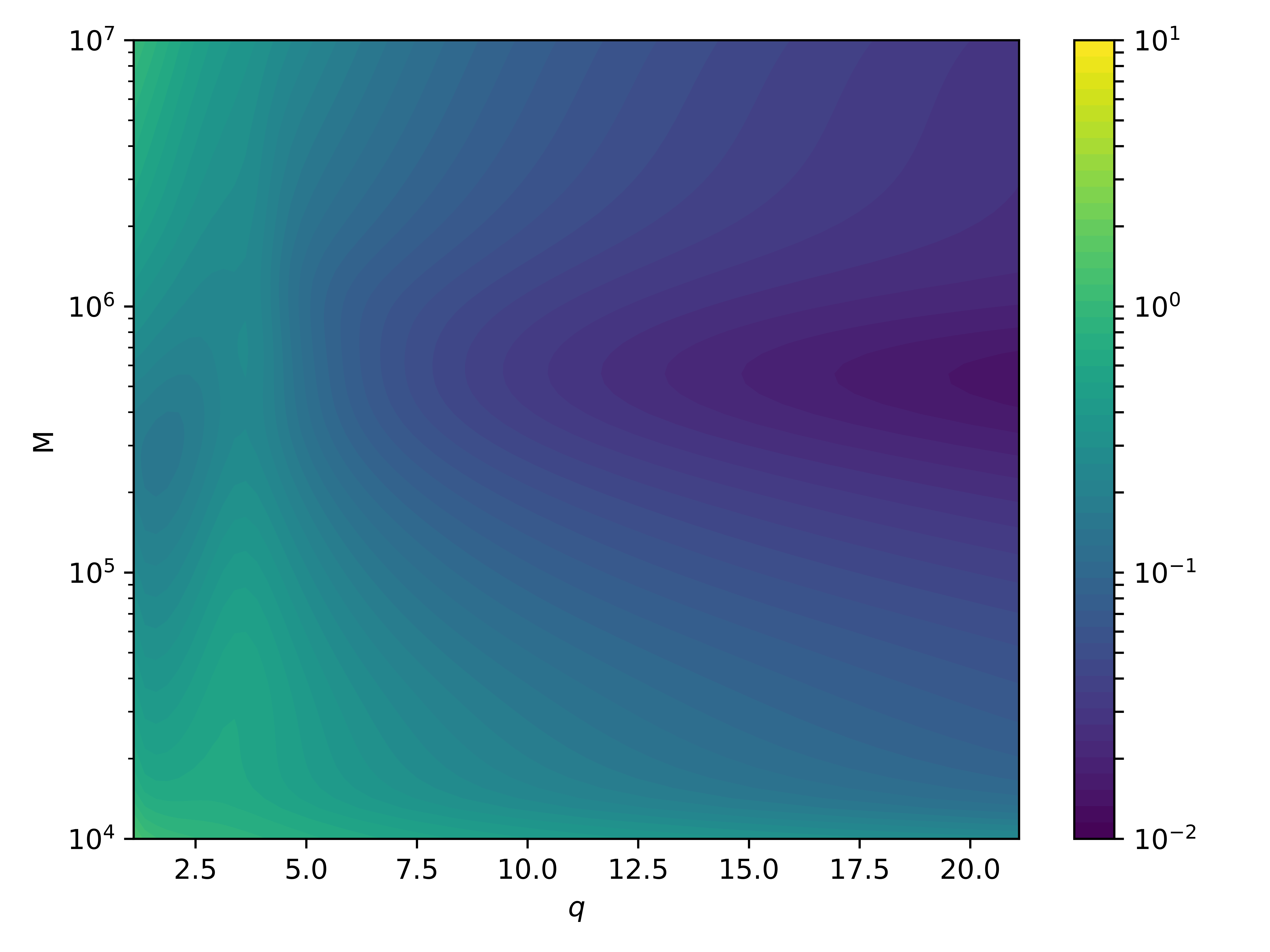
Figure 1: The contour plot for the PE accuracy of $\delta\kappa$ for different value of total mass and mass ratio for the duration of the signal equals to 1 day. The SNR for each point is normalized to 5000 by changing $D_{L}$ in TianQin over a coordinate of total mass and mass ratio and fixed SNR=5000.

According to the contour plot, we can find that TianQin has better capability for the sources around $10^{5.5}M_{\odot}$. This region corresponding to the most sensitivity band of TianQin. It also shows that the events with higher mass ratio will give a better constrain. This is consistent with the result of EMRI Zi et al. (2021), that the mass ratio become $10^{6}$ and the constraint of the SIQM reaches to the level of $10^{-4}$. For the events with asymmetric mass, the higher modes will become important. According to previous study, if we introduce the modification on the higher modes, the capability will also be improved Wang et al. (2023). We will show this in details with Bayesian analysis in next subsection.

III.2 Bayesian analysis

For the Bayesian analysis, we consider two kinds of injected data: the first one is the BBH signal with $\delta\kappa=0$, and the second one is the binary ECO signal with $\delta\kappa=10$. Both injections have three leading modes: $(2,2)$, $(2,1)$, and $(3,3)$, and the other parameters are chosen as Table 1. For the waveform used in the matched filtering, we didn’t assume the model of BBH, which means that $\delta\kappa$ is also a parameter need to be estimated that can’t be set as an constant. The marginalized probability distribution functions are shown in Fig 2. We can see that if we include the higher modes in the waveform, the capability will be improved for about 3 times. The PE result for all the parameters with BBH injected is shown in Fig 3 as an example. We can find that all the parameters are estimated properly, which means that all the true value are contained in the $1-\sigma$ region.

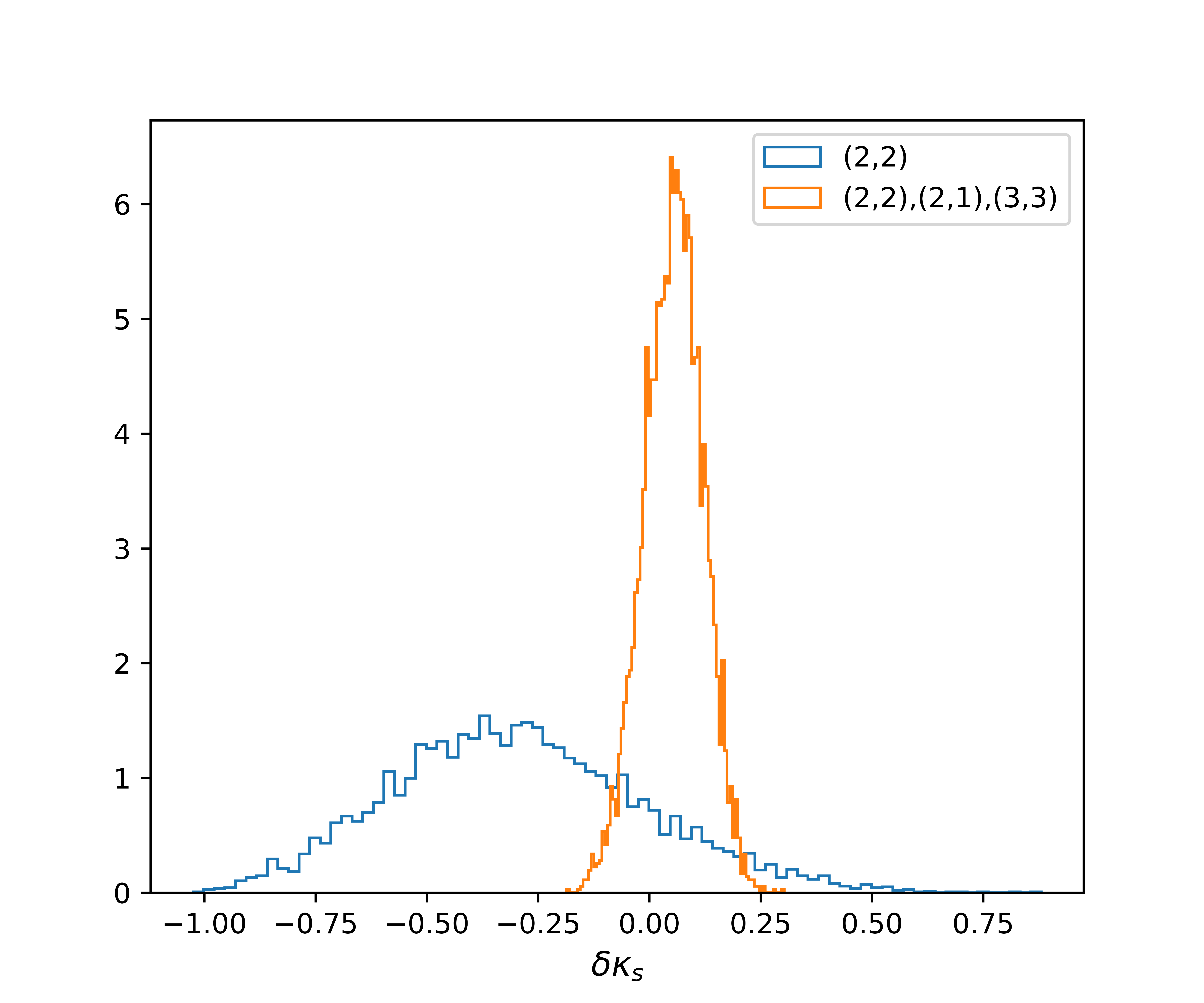
Figure 2: The PDF of $\delta\kappa_{s}$ for the wave form with $(2,2)$ mode only (blue) and with higher modes (orange). The top panel is the result for the injected signal with higher modes and $\delta\kappa_{s}=0$, The bottom panel is the resul for the injected signal with higher modes and $\delta\kappa_{s}=10$.

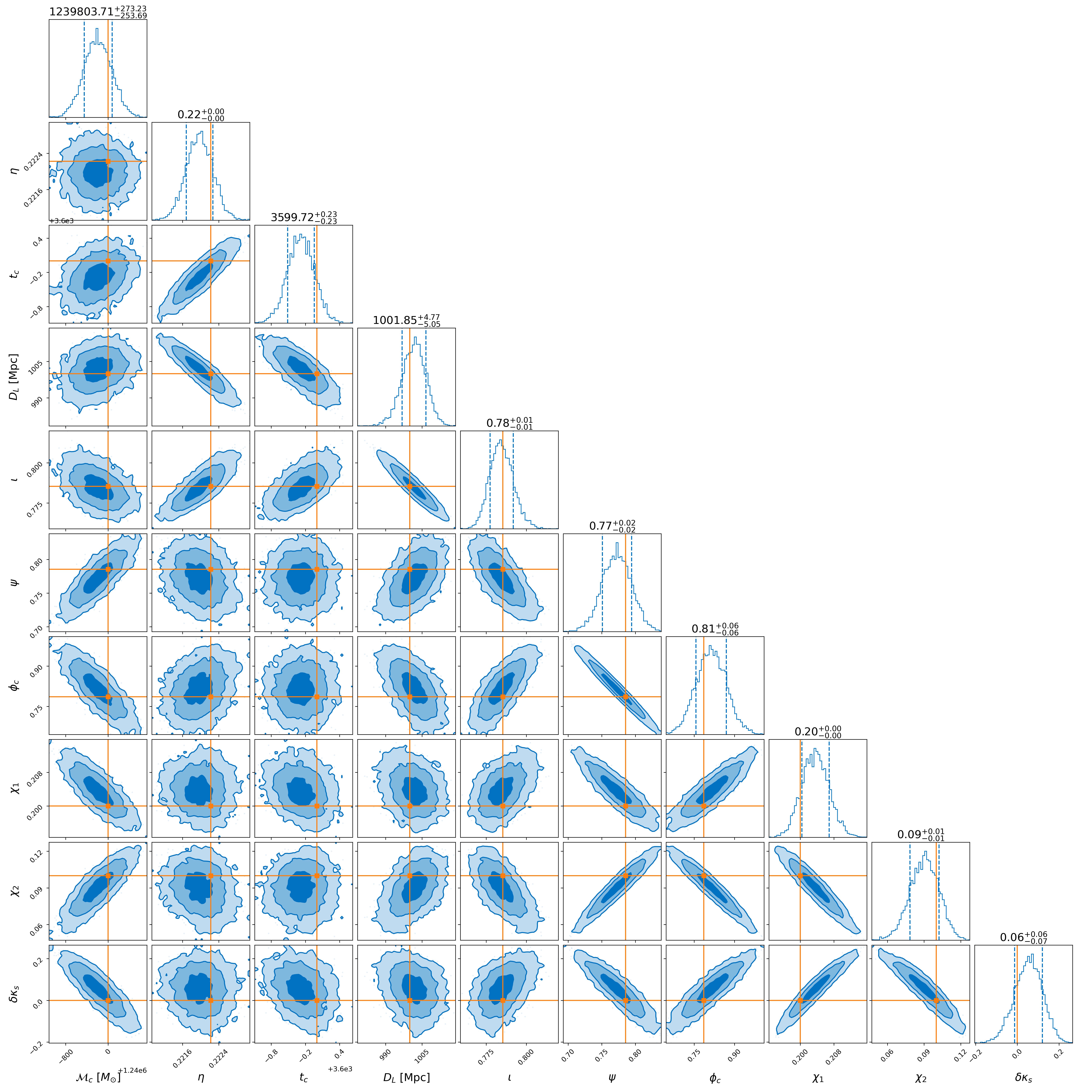
Figure 3: The PE result with higher modes included waveform, for the injected signal with higher modes and $\delta\kappa_{s}=0$. The SIQM is included in the estimated parameters.

We also analysis the case for a non-BBH injection with the estimation of BBH waveform. The injected value is $\delta\kappa=10$, and it’s fixed to be 0 in the Bayesian analysis. This corresponding to the real data is generated by a binary BS, but we mistakenly believed that it’s a BBH. The PE result is shown in Fig 4, we can see that all the parameters are estimated with a significant bias. For example, the injected value of the chirp mass equals to $1.24\times 10^{6}M_{\odot}$, but the estimated result is $1.25\times 10^{6}~{}^{+160}_{-163}M_{\odot}$, the true value is located at about $60-\sigma$ away from the point with the largest likelihood. This means that if we use the BBH waveform to fit a binary ECO signal, the parameters we estimated will have a significant deviation from the real value.

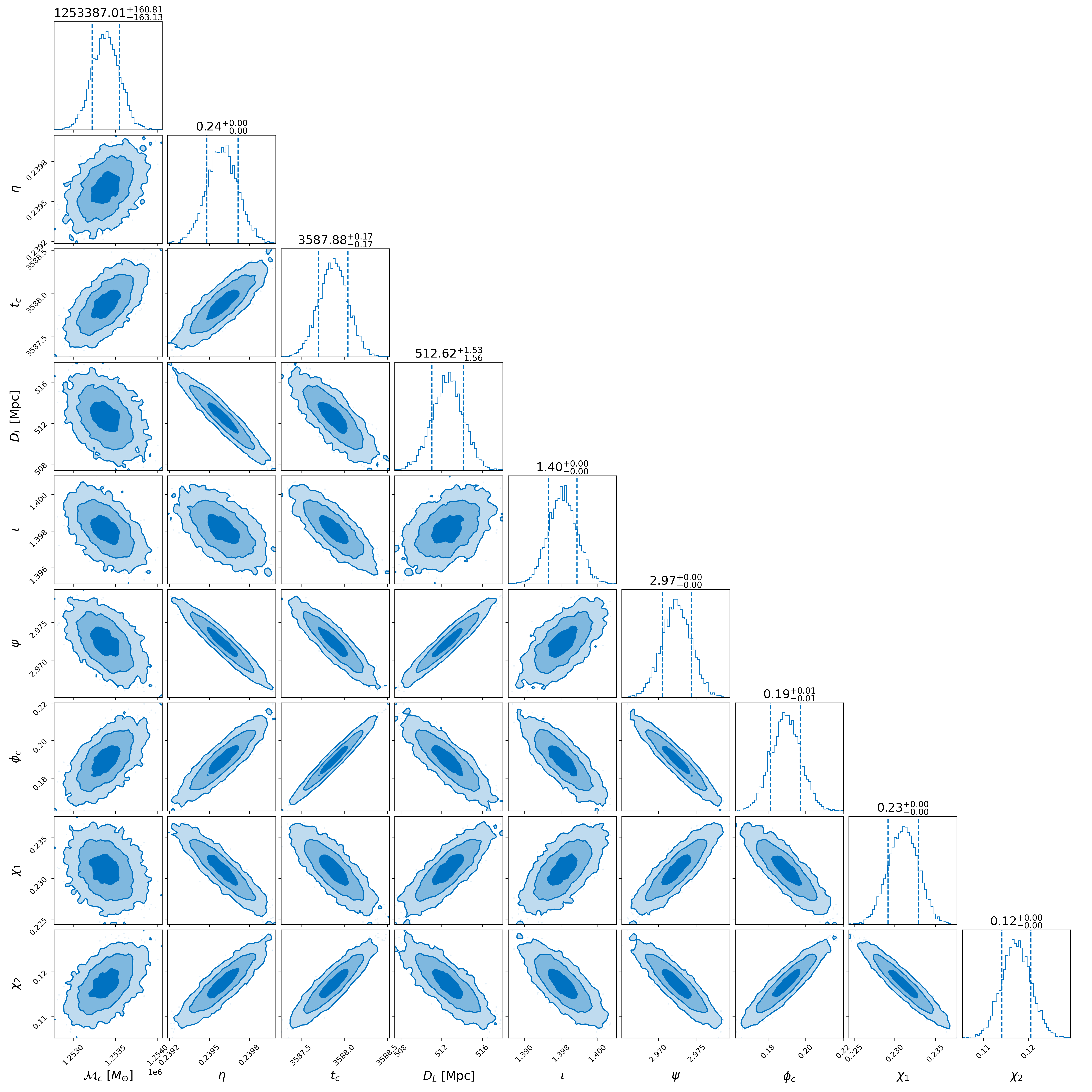
Figure 4: This figure demonstrates the corner plots of waveform template is also consistent to $\delta\kappa_{s}=0$ but the injected signal $\delta\kappa_{s}=10$ with 3 modes considered. We can easily notice that the estimated central values deviate from the injected values in the bottom figure which implies in this figure, our hypothesis is incorrect.

We also calculate the Bayes factors for the BH hypothesis compared to the ECO hypothesis. Here we analysed two kinds of injections, one is $\delta\kappa_{s}=0$ denotes the BH, the other is $\delta\kappa_{s}=10$ denotes the BS. The Bayes factor is calculated according to (19) for model 1 corresponding to BH and model 2 corresponding to ECO. Both injections include the higher modes, and we consider the case of estimate with $(2,2)$ mode only and higher modes included respectively.

Table 3: This table exhibits the $\lg\rm BF^{\rm BH}_{\rm ECO}$ with injected signal whose $\delta\kappa_{s}$=0 or 10 and with higher modes considered or not.

injected $\delta\kappa_{s}$	(2,2) mode only	include higher modes
0	0.19	1.49
10	-188.05	-4740.35

For the injection of BH, the results will favor the BH hypothesis, but the Bayes factor is not very large. $\rm log{\rm BF^{\rm BBH}_{\rm ECO}}$ will be 0.19 if we only consider the (2,2) mode, and the support on the true model is weak. But the result will increase to 1.49 if we consider the higher modes, and the support on the true model is strong. For the injection of ECO, the results will strongly favor the ECO hypothesis, and the Bayes factor will become very large. $\rm log{\rm BF^{\rm BBH}_{\rm ECO}}$ will be -188.05 if we only consider the (2,2) mode, and it will become -4740.35 if we consider the higher modes. Both results will support the true model with a very strong evidence. This means that we can distinguish the model of BH and ECO by calculating the Bayes factor, and then it can help us to avoid the possible systematic error.

IV Conclusion

The no-hair theorem requires that the multiple moments of a BH is fully determined by its mass and spin, and this relation will be violated for ECOs. This work focus on testing the no-hair theorem with the probing of the SIQM of the BHs using the inspiral signal of a BBH system. We consider the space-based GW detector TianQin as an example, and then the source is chose to be the MBHBs.

With the analysis with Fisher matrix, we find that TianQin has the best capability for the sources with the total mass around $10^{5}.5M_{\odot}$, corresponding to the sensitive band of TianQin. The result also shows that BBHs with larger mass ratio will have better constraint, and this implies the consideration of the higher modes.

Then we did the analysis with Bayesian inference. The result agrees with the estimation with Fisher matrix for both the model of BH and ECO, and the accuracy will be improved by about 3 times if we include the higher modes. We also find that if we use the BH model to inference the parameters of a binary ECO system, the estimation of the parameters will have very large systematic error. However, this can be avoid by the calculation of the Bayes factor, and the evidence will be strong enough to distinguish different models.

As a preliminary exploration, our work still have some limitations. For example, in the model with non-zero $\delta\kappa$, we have assumed both ECO in the binary system have the same value of $\delta\kappa$, and thus $\delta\kappa_{a}$ is fixed to zero. Obviously, this could not be the case in real world, but the degenerate between the parameters restrict us to estimate $\delta\kappa_{s}$ and $\delta\kappa_{a}$ simutaneously. Moreover, we use the data for only 1 day to do the PE to reduce the calculation. Although we have proved that this will not loss the generality, and the result will not change a lot for longer data. But this is not the case for the real data analysis, and the position of the source can’t be estimated for this case. We leave the inclusion and treatment of these more realistic issues for future exploration.

Appendix A The frequency for ISCO

In this appendix we present the formula corresponding the the ISCO frequency for BBH with spin Favata et al. (2022). The ISCO frequency can be written as

$$f_{\rm ISCO}=\frac{\hat{\Omega}(\chi_{f})}{\pi{M_{f}}},$$ (20)

where $\chi_{f}$ is the final spin, and $M_{f}$ is the final mass for the remant BH after the merger of BBH. The detailed calculation can be found in Husa et al. (2016); Hofmann et al. (2016). $\hat{\Omega}(\chi_{f})$ is the dimensionless ISCO Kerr angular frequency

$$\hat{\Omega}(\chi_{f})=\frac{1}{{\hat{r}_{\rm ISCO}}^{3/2}(\chi_{f})+\chi_{f}}$$ (21)

The dimensionless radius of the ISCO for a Kerr BH with dimensionless spin $\chi$ is

$$\begin{split}\hat{r}_{\rm ISCO}(\chi)=3+Z_{2}&-\frac{\chi}{|\chi|}\sqrt{(3-Z_{1})(3+Z_{1}+2Z_{2})}\\ &Z_{2}=\sqrt{3\chi^{2}+Z_{1}^{2}}\\ Z_{1}=1+(1-\chi^{2})&{}^{1/3}((1+\chi)^{1/3}+(1-\chi)^{1/3})\end{split}$$ (22)

References

- Abbott et al. (2016) B. P. Abbott, R. Abbott, T. Abbott, M. Abernathy, F. Acernese, K. Ackley, C. Adams, T. Adams, P. Addesso, R. Adhikari, et al., Physical review letters 116, 131103 (2016).
- Abbott et al. (2021a) R. Abbott, T. Abbott, S. Abraham, F. Acernese, K. Ackley, A. Adams, C. Adams, R. Adhikari, V. Adya, C. Affeldt, et al., Physical Review X 11, 021053 (2021a).
- Abbott et al. (2021b) R. Abbott et al., GWTC-3: Compact Binary Coalescences Observed by LIGO and Virgo During the Second Part of the Third Observing Run, arXiv 2111.03604 (2021b).
- Scientific (2021) L. Scientific, arXiv preprint arXiv:2108.01045 (2021).
- Abbott et al. (2019) B. Abbott, R. Abbott, T. Abbott, S. Abraham, F. Acernese, K. Ackley, C. Adams, R. X. Adhikari, V. Adya, C. Affeldt, et al., Physical Review D 100, 104036 (2019).
- Broekgaarden and Berger (2021) F. S. Broekgaarden and E. Berger, The Astrophysical Journal Letters 920, L13 (2021).
- Johnson-McDaniel et al. (2020) N. K. Johnson-McDaniel, A. Mukherjee, R. Kashyap, P. Ajith, W. Del Pozzo, and S. Vitale, Physical Review D 102, 123010 (2020).
- Haensel et al. (1986) P. Haensel, J. Zdunik, and R. Schaefer, Astronomy and Astrophysics (ISSN 0004-6361), vol. 160, no. 1, May 1986, p. 121-128. 160, 121 (1986).
- Kolb and Tkachev (1993) E. W. Kolb and I. I. Tkachev, Physical review letters 71, 3051 (1993).
- Mazur and Mottola (2023) P. O. Mazur and E. Mottola, Universe 9, 88 (2023).
- Cardoso and Pani (2019) V. Cardoso and P. Pani, Living Reviews in Relativity 22, 1 (2019).
- Hawking (2005) S. W. Hawking, Physical Review D 72, 084013 (2005).
- Blandford and Znajek (1977) R. D. Blandford and R. L. Znajek, Monthly Notices of the Royal Astronomical Society 179, 433 (1977).
- Hinderer et al. (2010) T. Hinderer, B. D. Lackey, R. N. Lang, and J. S. Read, Physical Review D 81, 123016 (2010).
- Chatziioannou (2020) K. Chatziioannou, General Relativity and Gravitation 52, 109 (2020).
- Raithel et al. (2018) C. A. Raithel, F. Özel, and D. Psaltis, The Astrophysical Journal Letters 857, L23 (2018).
- Malik et al. (2018) T. Malik, N. Alam, M. Fortin, C. Providência, B. Agrawal, T. Jha, B. Kumar, and S. Patra, Physical Review C 98, 035804 (2018).
- Bernuzzi et al. (2012) S. Bernuzzi, A. Nagar, and A. Zenginoğlu, Physical Review D 86, 104038 (2012).
- Kokkotas and Schmidt (1999) K. D. Kokkotas and B. G. Schmidt, Living Reviews in Relativity 2, 1 (1999).
- Kelly and Baker (2013) B. J. Kelly and J. G. Baker, Physical Review D 87, 084004 (2013).
- Ota and Chirenti (2020) I. Ota and C. Chirenti, Physical Review D 101, 104005 (2020).
- Baibhav et al. (2018) V. Baibhav, E. Berti, V. Cardoso, and G. Khanna, Physical Review D 97, 044048 (2018).
- Shi et al. (2019) C. Shi, J. Bao, H.-T. Wang, J.-d. Zhang, Y.-M. Hu, A. Sesana, E. Barausse, J. Mei, J. Luo, et al., Physical Review D 100, 044036 (2019).
- Berti et al. (2006) E. Berti, V. Cardoso, and C. M. Will, Physical Review D 73, 064030 (2006).
- Berti et al. (2007) E. Berti, J. Cardoso, V. Cardoso, and M. Cavaglia, Physical Review D 76, 104044 (2007).
- Dreyer et al. (2004) O. Dreyer, B. Kelly, B. Krishnan, L. S. Finn, D. Garrison, and R. Lopez-Aleman, Classical and Quantum Gravity 21, 787 (2004).
- Detweiler (1980) S. Detweiler, Astrophysical Journal, Part 1, vol. 239, July 1, 1980, p. 292-295. 239, 292 (1980).
- Poisson (1998) E. Poisson, Physical Review D 57, 5287 (1998).
- Kastha et al. (2018) S. Kastha, A. Gupta, K. Arun, B. Sathyaprakash, and C. Van Den Broeck, Physical Review D 98, 124033 (2018).
- Hansen (1974) R. O. Hansen, Journal of Mathematical Physics 15, 46 (1974).
- Geroch (1970) R. Geroch, Journal of Mathematical Physics 11, 2580 (1970).
- Thorne (1980) K. S. Thorne, Reviews of Modern Physics 52, 299 (1980).
- Compere et al. (2018) G. Compere, R. Oliveri, and A. Seraj, Journal of High Energy Physics 2018, 1 (2018).
- Krishnendu et al. (2017) N. Krishnendu, K. Arun, and C. K. Mishra, Physical review letters 119, 091101 (2017).
- Laarakkers and Poisson (1999) W. G. Laarakkers and E. Poisson, The Astrophysical Journal 512, 282 (1999).
- Pappas and Apostolatos (2012) G. Pappas and T. A. Apostolatos, Physical Review Letters 108, 231104 (2012).
- Stein et al. (2014) L. C. Stein, K. Yagi, and N. Yunes, The Astrophysical Journal 788, 15 (2014).
- Herdeiro and Radu (2014) C. A. Herdeiro and E. Radu, Physical review letters 112, 221101 (2014).
- Baumann et al. (2019) D. Baumann, H. S. Chia, and R. A. Porto, Physical Review D 99, 044001 (2019).
- Uchikata et al. (2016) N. Uchikata, S. Yoshida, and P. Pani, Physical Review D 94, 064015 (2016).
- Dubeibe et al. (2007) F. Dubeibe, L. A. Pachón, and J. D. Sanabria-Gómez, Physical Review D 75, 023008 (2007).
- Ryan (1997a) F. D. Ryan, Physical Review D 56, 1845 (1997a).
- Ryan (1997b) F. D. Ryan, Physical Review D 55, 6081 (1997b).
- Narikawa et al. (2021) T. Narikawa, N. Uchikata, and T. Tanaka, Physical Review D 104, 084056 (2021).
- Divyajyoti (2023) N. V. K. Divyajyoti, arXiv preprint arXiv:2311.05506 (2023).
- Abbott et al. (2021c) R. Abbott, H. Abe, F. Acernese, K. Ackley, N. Adhikari, R. Adhikari, V. Adkins, V. Adya, C. Affeldt, D. Agarwal, et al., arXiv preprint arXiv:2112.06861 (2021c).
- Abbott et al. (2021d) R. Abbott, T. Abbott, S. Abraham, F. Acernese, K. Ackley, A. Adams, C. Adams, R. X. Adhikari, V. Adya, C. Affeldt, et al., Physical review D 103, 122002 (2021d).
- Krishnendu and Yelikar (2020) N. Krishnendu and A. B. Yelikar, Classical and Quantum Gravity 37, 205019 (2020).
- Fan et al. (2020) H.-M. Fan, Y.-M. Hu, E. Barausse, A. Sesana, J.-d. Zhang, X. Zhang, T.-G. Zi, J. Mei, et al., Physical Review D 102, 063016 (2020).
- Zi et al. (2021) T. Zi, J.-d. Zhang, H.-M. Fan, X.-T. Zhang, Y.-M. Hu, C. Shi, J. Mei, et al., Physical Review D 104, 064008 (2021).
- Liu and Zhang (2020) M. Liu and J.-d. Zhang, arXiv preprint arXiv:2008.11396 (2020).
- Barack and Cutler (2004) L. Barack and C. Cutler, Physical Review D 69, 082005 (2004).
- Barack and Cutler (2007) L. Barack and C. Cutler, Physical Review D 75, 042003 (2007).
- Babak et al. (2017) S. Babak, J. Gair, A. Sesana, E. Barausse, C. F. Sopuerta, C. P. Berry, E. Berti, P. Amaro-Seoane, A. Petiteau, and A. Klein, Physical Review D 95, 103012 (2017).
- Luo et al. (2016) J. Luo, L.-S. Chen, H.-Z. Duan, Y.-G. Gong, S. Hu, J. Ji, Q. Liu, J. Mei, V. Milyukov, M. Sazhin, et al., Classical and Quantum Gravity 33, 035010 (2016).
- Hu et al. (2017) Y.-M. Hu, J. Mei, and J. Luo, National Science Review 4, 683 (2017).
- Mei et al. (2021) J. Mei, Y.-Z. Bai, J. Bao, E. Barausse, L. Cai, E. Canuto, B. Cao, W.-M. Chen, Y. Chen, Y.-W. Ding, et al., Progress of Theoretical and Experimental Physics 2021, 05A107 (2021).
- Wang et al. (2019) H.-T. Wang, Z. Jiang, A. Sesana, E. Barausse, S.-J. Huang, Y.-F. Wang, W.-F. Feng, Y. Wang, Y.-M. Hu, J. Mei, et al., Physical Review D 100, 043003 (2019).
- Feng et al. (2019) W.-F. Feng, H.-T. Wang, X.-C. Hu, Y.-M. Hu, and Y. Wang, Physical Review D 99, 123002 (2019).
- Liu et al. (2020) S. Liu, Y.-M. Hu, J.-d. Zhang, J. Mei, et al., Physical Review D 101, 103027 (2020).
- Liu et al. (2022) S. Liu, L.-G. Zhu, Y.-M. Hu, J.-D. Zhang, M.-J. Ji, et al., Physical Review D 105, 023019 (2022).
- Huang et al. (2020) S.-J. Huang, Y.-M. Hu, V. Korol, P.-C. Li, Z.-C. Liang, Y. Lu, H.-T. Wang, S. Yu, J. Mei, et al., Physical Review D 102, 063021 (2020).
- Fan et al. (2022) H.-M. Fan, S. Zhong, Z.-C. Liang, Z. Wu, J.-d. Zhang, and Y.-M. Hu, Phys. Rev. D 106, 124028 (2022), arXiv:2209.13387 [gr-qc] .
- Liang et al. (2023) Z.-C. Liang, Z.-Y. Li, E.-K. Li, J.-d. Zhang, and Y.-M. Hu, arXiv preprint arXiv:2307.01541 (2023).
- Liang et al. (2022) Z.-C. Liang, Y.-M. Hu, Y. Jiang, J. Cheng, J.-d. Zhang, J. Mei, et al., Physical Review D 105, 022001 (2022).
- Zhu et al. (2022a) L.-G. Zhu, Y.-M. Hu, H.-T. Wang, J.-d. Zhang, X.-D. Li, M. Hendry, and J. Mei, Phys. Rev. Res. 4, 013247 (2022a), arXiv:2104.11956 [astro-ph.CO] .
- Zhu et al. (2022b) L.-G. Zhu, L.-H. Xie, Y.-M. Hu, S. Liu, E.-K. Li, N. R. Napolitano, B.-T. Tang, J.-d. Zhang, and J. Mei, Sci. China Phys. Mech. Astron. 65, 259811 (2022b), arXiv:2110.05224 [astro-ph.CO] .
- Huang et al. (2023) S.-J. Huang, Y.-M. Hu, X. Chen, J.-d. Zhang, E.-K. Li, Z. Gao, and X.-Y. Lin, JCAP 08, 003 (2023), arXiv:2304.10435 [astro-ph.CO] .
- Bao et al. (2019) J. Bao, C. Shi, H. Wang, J.-d. Zhang, Y. Hu, J. Mei, J. Luo, et al., Physical Review D 100, 084024 (2019).
- Sun et al. (2023) S. Sun, C. Shi, J.-d. Zhang, and J. Mei, Phys. Rev. D 107, 044023 (2023), arXiv:2207.13009 [gr-qc] .
- Xie et al. (2022) N. Xie, J.-d. Zhang, S.-J. Huang, Y.-M. Hu, and J. Mei, Phys. Rev. D 106, 124017 (2022), arXiv:2208.10831 [gr-qc] .
- Shi et al. (2023) C. Shi, M. Ji, J.-d. Zhang, and J. Mei, Phys. Rev. D 108, 024030 (2023), arXiv:2210.13006 [gr-qc] .
- Lin et al. (2023) X.-y. Lin, J.-d. Zhang, L. Dai, S.-J. Huang, and J. Mei, Phys. Rev. D 108, 064020 (2023), arXiv:2304.04800 [gr-qc] .
- García-Quirós et al. (2020) C. García-Quirós, M. Colleoni, S. Husa, H. Estellés, G. Pratten, A. Ramos-Buades, M. Mateu-Lucena, and R. Jaume, Physical Review D 102, 064002 (2020).
- Arun et al. (2009) K. Arun, A. Buonanno, G. Faye, and E. Ochsner, Physical Review D 79, 104023 (2009).
- Mishra et al. (2016) C. K. Mishra, A. Kela, K. Arun, and G. Faye, Physical Review D 93, 084054 (2016).
- Mezzasoma and Yunes (2022) S. Mezzasoma and N. Yunes, Physical Review D 106, 024026 (2022).
- Tinto et al. (2004) M. Tinto, F. B. Estabrook, and J. W. Armstrong, Phys. Rev. D 69, 082001 (2004), arXiv:gr-qc/0310017 .
- Marsat et al. (2021) S. Marsat, J. G. Baker, and T. Dal Canton, Physical Review D 103, 083011 (2021).
- Lyu et al. (2023) X. Lyu, E.-K. Li, Y.-M. Hu, et al., Physical Review D 108, 083023 (2023).
- Cutler and Flanagan (1994) C. Cutler and E. E. Flanagan, Physical Review D 49, 2658 (1994).
- Thrane and Talbot (2019) E. Thrane and C. Talbot, Publications of the Astronomical Society of Australia 36, e010 (2019).
- Ashton et al. (2019) G. Ashton, M. Hübner, P. D. Lasky, C. Talbot, K. Ackley, S. Biscoveanu, Q. Chu, A. Divakarla, P. J. Easter, B. Goncharov, et al., The Astrophysical Journal Supplement Series 241, 27 (2019).
- Speagle (2020) J. S. Speagle, Monthly Notices of the Royal Astronomical Society 493, 3132 (2020).
- Skilling (2006) J. Skilling, Bayesian Analysis 1, 833 (2006).
- Wang et al. (2023) B. Wang, C. Shi, J.-d. Zhang, Y.-M. hu, and J. Mei, Phys. Rev. D 108, 044061 (2023), arXiv:2302.10112 [gr-qc] .
- van der Walt et al. (2011) S. van der Walt, S. C. Colbert, and G. Varoquaux, Comput. Sci. Eng. 13, 22 (2011), arXiv:1102.1523 [cs.MS] .
- Virtanen et al. (2020) P. Virtanen et al., Nature Meth. 17, 261 (2020), arXiv:1907.10121 [cs.MS] .
- Hunter (2007) J. D. Hunter, Comput. Sci. Eng. 9, 90 (2007).
- Foreman-Mackey (2016) D. Foreman-Mackey, Journal of Open Source Software 1, 24 (2016).
- Favata et al. (2022) M. Favata, C. Kim, K. Arun, J. Kim, and H. W. Lee, Physical Review D 105, 023003 (2022).
- Husa et al. (2016) S. Husa, S. Khan, M. Hannam, M. Pürrer, F. Ohme, X. J. Forteza, and A. Bohé, Physical Review D 93, 044006 (2016).
- Hofmann et al. (2016) F. Hofmann, E. Barausse, and L. Rezzolla, The Astrophysical Journal Letters 825, L19 (2016).