Scalable Automated Verification for Cyber-Physical Systems in Isabelle/HOL Jonathan Julián Huerta y Munive Czech Institute of Informatics, Robotics and Cybernetics Prague, Czechia Simon Foster University of York United Kingdom Mario Gleirscher University of Bremen Germany Georg Struth University of Sheffield United Kingdom Christian Pardillo Laursen University of York United Kingdom Thomas Hickman Genomics PLC United Kingdom (22/January/2024) Abstract We formally introduce IsaVODEs (Isabelle verification with Ordinary Differential Equations), a framework for the verification of cyber-physical systems. We describe the semantic foundations of the framework’s formalisation in the Isabelle/HOL proof assistant. A user-friendly language specification based on a robust state model makes our framework flexible and adaptable to various engineering workflows. New additions to the framework increase both its expressivity and proof automation. Specifically, formalisations related to forward diamond correctness specifications, certification of unique solutions to ordinary differential equations (ODEs) as flows, and invariant reasoning for systems of ODEs contribute to the framework’s scalability and usability. Various examples and an evaluation validate the effectiveness of our framework. Keywords: cyber-physical systems, hybrid systems, program verification, interactive theorem proving, predicate transformers, lenses 1 Introduction Cyber-physical systems (CPSs) are computerised systems whose software (the “cyber” part) interacts with their physical environment. The software is modelled as a variable-updating, potentially non-deterministic program, while the environment is modelled by a system of ordinary differential equations (ODEs). When CPSs interact with humans, for example through robotic manipulators, they are invariably safety-critical, which makes their design verification imperative. However, CPS verification is challenging because of the complex interactions between the software, hardware, and the physical environment. These produce uncountably infinite state spaces, which makes verification generally intractable, and so requires the use of abstractions. A deductive verification approach uses symbolic logics, which support the encoding of solutions and invariants of ODEs. Such an approach has been implemented with the KeYmaera X tool (KYX) [31], which models CPSs via hybrid programs, and verifies their behaviour with differential dynamic logic (𝖽ℒ𝖽ℒ\mathsf{d}\mathcal{L}). Numerous case studies and competitions support the applicability of this approach [44, 52, 56, 85]. General-purpose interactive theorem provers (ITPs), like Coq, Lean, and Isabelle, also support CPS verification [40, 25]. Their track record for large-scale deductive verification is well-documented [5, 14, 45, 47, 49]. A significant reason for these successes is the combination of expressive logical languages, and plugins to enhance reasoning capacity and usability. Different from bespoke axiomatic provers like KYX, these tools are inherently extensible since the mathematics is constructed from first principles, rather than postulated, with accompanying soundness guarantees. For example, the recent addition of transcendental functions to KYX necessitated an extension of the tool, whereas these have been available in HOL, Coq, and Isabelle for many years. Moreover, the foundational mathematical libraries are under constant development by the community111See Isabelle’s Archive of Formal Proofs (https://www.isa-afp.org/statistics/) and Lean’s Mathematical Library (https://leanprover-community.github.io/mathlib_stats.html)., and so ITP-based verification tools benefit from an ever-growing library of definitions and theorems. Our ITP of choice, Isabelle/HOL, provides a framework supporting assured software engineering [45, 11], through an open extensible architecture; a flexible syntax pipeline [82, 60]; integration of external analysis tools in Sledgehammer, Nitpick, and cousins; and output of software artefacts in a variety of languages [34]. Isabelle’s rich library for multi-variate analysis (HOL-Analysis) can be applied to CPS verification [37, 42]. Thanks to its higher-order logic, Isabelle supports several modelling facilities essential to control engineering, such as vectors, matrices, and transcendental functions (e.g. sin\sin, cos\cos, and exsuperscript𝑒𝑥e^{x}) [8, 38], and it has extended reasoning capability through its integration with SMT solvers (CVC4, Z3, Vampire) [61]. Isabelle is therefore ideally suited to reasoning about CPSs, but to harness its facilities we need an accessible and powerful CPS modelling language and verification framework. In this paper we contribute an Isabelle-based verification framework called IsaVODEs (Isabelle Verification with Ordinary Differential Equations) [40, 25]. IsaVODEs provides a textual language for modelling CPSs, which is constructed as a shallow embedding in Isabelle. The language is equipped with nondeterministic state-transformer-based program semantics and a flexible hybrid store model based on lenses [23, 27]. The program model provides several verification calculi, including Hoare logic and dynamic logic, with modalities for specifying both safety and reachability properties. The store model allows software models to benefit from the full generality of the Isabelle type system, including continuous structures like vectors and matrices, and discrete structures like algebraic data types. Our language can therefore scale to systems with both realistic dynamics, and complex control structures. We harness Isabelle’s syntax translation mechanisms to provide a user-friendly frontend for the language, including declarative context, program notation, and operators for arithmetic, vectors, and matrices. Our technical solution is extensible and endeavours to resemble languages like Modelica, Mathematica, and MATLAB. Verification of models in IsaVODEs is supported by a library of deduction rules. For reasoning about ODEs, we support both the use of solutions with flow functions, and differential induction, which avoids the need for solutions. We integrate two Computer Algebra Systems (CASs), namely Mathematica and SageMath, into Isabelle for the supply of symbolic solutions to Lipschitz-continuous ODEs in an analogous way to sledgehammer. We also support both a 𝖽ℒ𝖽ℒ\mathsf{d}\mathcal{L}-style differential ghost rule and Darboux rules that enhance IsaVODEs’ invariant reasoning capabilities for complex continuous dynamics. Orthogonal to this, we also contribute novel laws to support local reasoning in the style of separation logic. We can infer the frame of a program (i.e. the mutable variables), and use a frame rule to prove invariants over variables outside the frame. This is accompanied by a novel form of differentiation called “framed Fréchet derivatives”, which allow us to differentiate with respect to a strict subset of the store variables, particularly ignoring any discrete variables lacking a topological structure. When variables are outside of the frame of a system of ODEs, those variables are unchanged during continuous evolution. Local reasoning further facilitates scalability of our tool, by allowing a verification task to be decomposed into modules supported by individual assumptions and guarantees. We supply several proof methods to support automated proof and verification condition generation (VCG), including the application of differential induction, certification of ODE solutions, and the various Hoare-logic laws. Care is taken to ensure that the resulting proof obligations are presented in a way that preserves abstraction, and elides irrelevant details of the Isabelle mechanisation, to maintain the user experience. Harnessing Isabelle’s Eisbach tool [53], we also employ various high-level search-based proof methods, which exhaustively apply the proof rules to compute a complete set of VCs. The VCs can finally be tackled in the usual way using tools like auto and sledgehammer. The framework has been tested successfully on a large set of hybrid verification benchmarks [54], and many larger examples. Our enhancements yield at least the same performance in essential verification tasks as that of domain-specific provers. Initial case studies suggest a simplification of user interaction. Our new components can be found online222github.com/isabelle-utp/Hybrid-Verification, also by clicking our icons .. Our contributions are highlighted through examples, while additional contributions are noted throughout the text. This article is a substantial extension of previously published work at the Formal Methods symposium (FM2021) [27]. Our additional contributions include generalisations of the laws for frames (§5.1), differential ghosts, and Darboux rules (§5.4); proof methods for certification of continuity, Lipschitz continuity, and uniqueness of solutions (§6.2); extensions to our previous proof methods (§6); the CAS integrations (§6.5); a more substantial evaluation (§7); and several additional examples (§2, §8). As a result of these enhancements, the usability of the tool is more mature and polished. We begin our paper by illustrating the framework with a small case study (§2). We then expound our formalisation of dynamical systems (§3.1), the state-transformer hybrid program model (§3.2), the foundations of the store model (§3.3), the specification of continuous evolution (§3.4), and finally VCG though our framework’s algebraic foundations (§3.5). This includes both safety, and also reachability and termination (§3.5.3). Next, in §4, we introduce our framework’s hybrid modelling language. We supply commands for generating hybrid stores, with variables, constants, and foundational properties (§4.1), and user-friendly notation for expressions (§4.3), matrices, and vectors (§4.4). The notation is automatically processed via rewriting rules supplied to Isabelle’s simplifier, hiding implementation details. In §5 we present laws for local reasoning about frames (§5.1), the seamless integration of framed ODEs into our hybrid programs (§5.2), and automatic certification of ODE invariants through framed Fréchet derivatives (§5.3). These also serve to supply new 𝖽ℒ𝖽ℒ\mathsf{d}\mathcal{L}-style ghost and Darboux rules that enhance IsaVODEs’ invariant reasoning (§5.4). We contribute increased IsaVODEs proof-capabilities for the verification process. We formalise theorems necessary for increased automation, like the fact that differentiable functions are Lipschitz-continuous (§6.2) or the first and second derivative test laws (§6.7). We provide methods to automate certification of differentiation (§6.1), uniqueness of solutions (§6.3), invariants for ODEs (§6.6), and VCG (§6.4). Additional automation is provided through the integration of Mathematica and SageMath (§6.5). We then bring all of the results together for the evaluation (§7) using benchmarks and examples (§8). In the remaining sections we review related work (§9), provide concluding statements, and discuss future research avenues (§10). 2 Motivating Case Study: Flight Dynamics (a) Plane x and y position (b) Velocities and angle (c) Evasive maneuvers (d) Collision Figure 1: Diagrams illustrating the flight dynamics example In this section, we motivate and demonstrate our framework’s usage with a worked example: an aircraft collision avoidance scenario that was first presented by Mitsch et. al. [55]. It describes an aircraft trying to avoid a collision with a nearby intruding aircraft travelling at the same altitude. We can model this intruding aircraft by considering its coordinates x𝑥x and y𝑦y, and angle ϑitalic-ϑ\vartheta, in the reference frame of our own ship. The intruding plane has fixed velocity vi>0subscript𝑣𝑖0v_{i}>0, and our plane has fixed velocity vo>0subscript𝑣𝑜0v_{o}>0 and variable angular velocity ω𝜔\omega. This is illustrated in Figure 1(a) and 1(b). With our tool, we can model this using a dataspace command, as shown below: dataspace planar_flight = constants vo :: real (* own_velocity *) vi :: real (* intruder velocity *) assumes vo_pos: "vo > 0" and vi_pos: "vi > 0" variables (* Coordinates in reference frame of own ship *) x :: real (* Intruder x *) y :: real (* Intruder y *) θ𝜃\theta :: real (* Intruder angle *) ω𝜔\omega :: real (* Angular velocity *) This command allows us to define our constants, any assumptions about the verification problem, and the system’s variables. In this case, we postulate two constants vosubscript𝑣𝑜v_{o} and visubscript𝑣𝑖v_{i}, both of type real, for the velocity of the aircraft and intruder, respectively. Here, real is the type of precise mathematical real numbers, as opposed to floating points or rationals. As per the problem statement, we assume that both of these constants are strictly positive. This is specified by the assumptions called vo_pos and vi_pos, respectively, which can be used as hypotheses in proofs. We supply the variables of this system, which give the relative position of the intruder (x and y), its orientation θ𝜃\theta, and its angular velocity ω𝜔\omega. We next specify the ODEs that model the system as a constant called plant: definition "plant ≡\equiv {x‘ = vi * cos θ𝜃\theta - vo + ω𝜔\omega * y, y‘ = vi * sin θ𝜃\theta - ω𝜔\omega * x, θ𝜃\theta‘ = -ω𝜔\omega}" The ODEs can be specified in a user-friendly manner, as physicists and engineers would informally state them, in terms of the constants and variables of the system x, y, and φ𝜑\varphi. Next, we define a simple controller to avoid collisions, as explained below: abbreviation "I ≡\equiv (vi * sin θ𝜃\theta * x - (vi * cos θ𝜃\theta - vo) * y > vo + vi)e" abbreviation "J ≡\equiv (vi * ω𝜔\omega * sin θ𝜃\theta * x - vi * ω𝜔\omega * cos θ𝜃\theta * y + vo * vi * cos θ𝜃\theta > vo * vi + vi * ω𝜔\omega)e" definition "ctrl ≡\equiv (ω𝜔\omega ::= 0; ¿I?) ⊓square-intersection\sqcap (ω𝜔\omega ::= 1; ¿J?)" This is based on two invariants, I𝐼I and J𝐽J, for two different scenarios. These are properties that remain true after the unfolding of each scenario. The invariant I𝐼I holds when going straight is safe, while J𝐽J holds when an evasion manoeuvre is allowed. Our controller selects whether to set our aircraft’s angular velocity to 0 or 1 depending on which invariant holds (I𝐼I and J𝐽J respectively). The evasive manoeuvres that occur when the angular velocity is set to 1 are illustrated in figure 1(c). Finally, our model follows the usual structure of an iteration (∗) of control choices (ctrl) followed by a nondeterministic evolution of the system dynamics (plant): definition "flight ≡\equiv (ctrl; plant)∗" The behaviour of the system is characterised by all states reachable by executing the controller followed by the plant a finite number of times. Next, we show how we can formally verify the collision avoidance of this system. We do this by specifying a Hoare triple within an Isabelle lemma: lemma flight_safe: "{x2 + y2 > 0} flight {x2 + y2 > 0}" proof - have ctrl_post: "{x2 + y2 > 0} ctrl {(ωω\omega = 0 ∧\wedge @I) ∨\vee (ωω\omega = 1 ∧\wedge @J)}" unfolding ctrl_def by wlp_full have plant_safe_I: "{ωω\omega = 0 ∧\wedge @I} plant {x2 + y2 > 0}" unfolding plant_def apply (dInv "($ωω\omega = 0 ∧\wedge @I)e", dWeaken) using vo_pos vi_pos sum_squares_gt_zero_iff by fastforce have plant_safe_J: "{ωω\omega = 1 ∧\wedge @J} plant {x2 + y2 > 0}" unfolding plant_def apply (dInv "(ωω\omega=1 ∧\wedge @J)e", dWeaken) by (smt (z3) cos_le_one mult_if_delta mult_le_cancel_iff2 mult_left_le sum_squares_gt_zero_iff vi_pos vo_pos) show ?thesis unfolding flight_def apply (intro hoare_kstar_inv hoare_kcomp[OF ctrl_post]) by (rule hoare_disj_split[OF plant_safe_I plant_safe_J]) qed We formulate collision avoidance using x2+y2>0superscript𝑥2superscript𝑦20x^{2}+y^{2}>0 as the invariant in the Hoare triple. A collision occurs when x2+y2=0superscript𝑥2superscript𝑦20x^{2}+y^{2}=0, as illustrated in figure 1(d). We use Isabelle’s Isar scripting language to break down the verification into several intermediate properties via the Isar command “have”, which takes a label followed by a property specification. We first calculate the postconditions that arise from running the controller (ctrl) by using our tactic wlp_full (see Section 6). This gives us two possible execution branches – one where I∧ω=0𝐼𝜔0I\land\omega=0 holds, and one where J∧ω=1𝐽𝜔1J\land\omega=1 holds. We give this first property the name ctrl_post. The postconditions provide two possible initial states for the plant, which we consider using the properties plant_safe_I and plant_safe_J. We show that both preconditions guarantee the problem’s postcondition x2+y2>0superscript𝑥2superscript𝑦20x^{2}+y^{2}>0 by applying differential induction, a technique that proves an invariant of a system of ODEs without computing a solution (see Section 5.3). In each case, we use our Eisbach-designed method dInv, which takes as a parameter the invariant we wish to prove. The invariant is simply the precondition of each Hoare triple. However, we then need to prove that this invariant implies the postcondition, which is done using a further method called dWeaken. The remaining proof obligations can be solved using the Sledgehammer tool, which calls external automated theorem provers to find a solution and reconstructs it using the names of previously proven theorems in Isabelle’s libraries. In particular, the property plant_safe_J is discharged using Z3, which uses trigonometric identities formalised in HOL-Analysis. We display the proof state resulting from applying differential induction below: In the case that Sledgehammer is unable to find a proof, this proof obligation is quite readable, and so a manual proof or refutation could be given (See Section 8). Finally, we put everything together to show that the whole system is safe, using the Isar command show, which is used to conclude proofs and restate the overall goal of the lemma (?thesis). The proof uses a couple of high-level Hoare logic laws, and the properties that were proven to complete the proof. This final step can be completely automated using Isabelle’s classical reasoner, but we leave the details for the purpose of demonstration. This completes our overview of our tool and its capabilities. In the remainder of the paper, we will expound the technical foundations of the tool, and our key results. 3 Semantics for hybrid systems verification We start the section by recapitulating basic concepts from the theory of dynamical systems. We use these notions to describe our approach [40, 27] to hybrid systems verification in general-purpose proof assistants. Specifically, we present hybrid programs and their state transformer semantics. We then introduce our store model and provide intuitions for deriving state transformers for program assignments and ODEs relative to this model. We extend our approach to a predicate transformer semantics to derive laws for verification condition generation (VCG) [40, 9]. That is, we introduce the forward box predicate transformer and use its properties to derive the rules of Hoare logic. Finally, we introduce the forward diamond predicate transformer which serves to prove reachability and progress properties of hybrid systems. Our formalisation of these concepts as a shallow embedding in Isabelle/HOL maximises the availability of the prover’s proof automation in VCG. 3.1 Dynamical Systems In this section, we consider two ways to specify continuous dynamical systems [78]: explicitly via flows and implicitly via systems of ordinary differential equations (ODEs). Flows are functions φ:T→𝒞→𝒞:𝜑→𝑇𝒞→𝒞\varphi:T\to\mathcal{C}\to\mathcal{C}, where T𝑇T is a non-discrete submonoid of the real numbers ℝℝ\mathbb{R} representing time. Similarly, 𝒞𝒞\mathcal{C} is a set with some topological structure like a vector space or a metric space. We emphasise this intuition using an overhead arrow for elements c→∈𝒞→𝑐𝒞\vec{c}\in\mathcal{C} and refer to 𝒞𝒞\mathcal{C} as a continuous state space. By definition, flows are continuously differentiable (C1superscript𝐶1C^{1}) functions and monoid actions: they satisfy the laws φ(t1+t2)=φt1∘φt2𝜑subscript𝑡1subscript𝑡2𝜑subscript𝑡1𝜑subscript𝑡2\varphi(t_{1}+t_{2})=\varphi\,t_{1}\circ\varphi\,t_{2} and φ 0=𝑖𝑑𝒞𝜑 0subscript𝑖𝑑𝒞\varphi\,0=\mathit{id}_{\mathcal{C}}. Given a state c→∈𝒞→𝑐𝒞\vec{c}\in\mathcal{C}, the trajectory φc→:T→𝒞:subscript𝜑→𝑐→𝑇𝒞\varphi_{\vec{c}}:T\to\mathcal{C}, such that φc→t=φtc→subscript𝜑→𝑐𝑡𝜑𝑡→𝑐\varphi_{\vec{c}}\,t=\varphi\,t\,\vec{c}, is a curve modelling the continuous dynamical system’s evolution in time and passing through c→→𝑐\vec{c}. The orbit map γφ:𝒞→𝒫𝒞:superscript𝛾𝜑→𝒞𝒫𝒞\gamma^{\varphi}:\mathcal{C}\to\operatorname{\mathcal{P}}\,\mathcal{C}, such that γφc→=𝒫φc→Tsuperscript𝛾𝜑→𝑐𝒫subscript𝜑→𝑐𝑇\gamma^{\varphi}\,\vec{c}=\operatorname{\mathcal{P}}\,\varphi_{\vec{c}}\,T, gives the graph of this curve for c→→𝑐\vec{c}, where 𝒫𝒫\operatorname{\mathcal{P}} denotes both the powerset operation and the direct image operator. Systems of ODEs are related to flows through their solutions. Formally, systems of ODEs are specified by vector fields f:T→𝒞→𝒞:𝑓→𝑇𝒞→𝒞f:T\rightarrow\mathcal{C}\rightarrow\mathcal{C}, functions assigning vectors to points in space-time. A solution X:T→𝒞:𝑋→𝑇𝒞X:T\to\mathcal{C} to the system of ODEs specified by f𝑓f is then a C1superscript𝐶1C^{1}-function such that X′t=ft(Xt)superscript𝑋′𝑡𝑓𝑡𝑋𝑡X^{\prime}\,t=f\,t\,(X\,t) for all t𝑡t in some interval U⊆T𝑈𝑇U\subseteq T. This solution also solves the associated initial value problem (IVP) given by (t0,c→)subscript𝑡0→𝑐(t_{0},\vec{c}) (denoted by X∈𝑖𝑣𝑝-𝑠𝑜𝑙𝑠Uft0c→𝑋𝑖𝑣𝑝-𝑠𝑜𝑙𝑠𝑈𝑓subscript𝑡0→𝑐X\in\mathit{ivp}\texttt{-}\mathit{sols}\,U\,f\,t_{0}\,\,\vec{c}) if it satisfies Xt0=c→𝑋subscript𝑡0→𝑐X\,t_{0}=\vec{c}, with t0∈Usubscript𝑡0𝑈t_{0}\in U. The existence of solutions to IVPs is guaranteed for continuous vector fields by the Peano theorem, albeit on an interval Uc→𝑈→𝑐U\,\vec{c} depending on the initial condition (t0,c→)subscript𝑡0→𝑐(t_{0},\vec{c}). Similarly, the Picard-Lindelöf theorem states that all solutions to the IVP X′t=ft(Xt)superscript𝑋′𝑡𝑓𝑡𝑋𝑡X^{\prime}\,t=f\,t\,(X\,t) with Xt0=c→𝑋subscript𝑡0→𝑐X\,t_{0}=\vec{c} coincide in some interval Uc→⊆T𝑈→𝑐𝑇U\,\vec{c}\subseteq T (around t0subscript𝑡0t_{0}) if f𝑓f is Lipschitz continuous on T𝑇T. In other words, it states that there is a unique solution to the IVP on Uc→𝑈→𝑐U\,\vec{c}. Thanks to this, when f𝑓f is Lipschitz continuous on T𝑇T, t0=0subscript𝑡00t_{0}=0, and Uc→=T𝑈→𝑐𝑇U\,\vec{c}=T for all c→∈𝒞→𝑐𝒞\vec{c}\in\mathcal{C}, the solutions to the associated IVPs are exactly a flow’s trajectories φc→subscript𝜑→𝑐\varphi_{\vec{c}}, that is, φc→′t=ft(φc→t)superscriptsubscript𝜑→𝑐′𝑡𝑓𝑡subscript𝜑→𝑐𝑡\varphi_{\vec{c}}^{\prime}\,t=f\,t\,(\varphi_{\vec{c}}\,t) and φc→ 0=c→subscript𝜑→𝑐 0→𝑐\varphi_{\vec{c}}\,0=\vec{c}. Therefore, the flow φ𝜑\varphi is the function mapping to each c→∈𝒞→𝑐𝒞\vec{c}\in\mathcal{C} the unique φc→subscript𝜑→𝑐\varphi_{\vec{c}} such that φc→∈𝑖𝑣𝑝-𝑠𝑜𝑙𝑠Tf 0c→subscript𝜑→𝑐𝑖𝑣𝑝-𝑠𝑜𝑙𝑠𝑇𝑓 0→𝑐\varphi_{\vec{c}}\in\mathit{ivp}\texttt{-}\mathit{sols}\,T\,f\,0\,\,\vec{c}. Example 1. We illustrate the above properties about flows and ODEs with the differential equation y′t=a⋅yt+bsuperscript𝑦′𝑡⋅𝑎𝑦𝑡𝑏y^{\prime}\,t=a\cdot y\,t+b, where a≠0𝑎0a\neq 0 and t∈ℝ𝑡ℝt\in\mathbb{R}. This is an important ODE modelling for instance idealised bacterial growth [76], radioactive decay [81] or concentration of glucose in the blood (without the intervention of insulin) [2]. First, given that differentiability implies Lipschitz continuity [78], we can verify that this equation has unique solutions (by the Picard-Lindelöf theorem) simply by noticing that ft=a⋅yt+b𝑓𝑡⋅𝑎𝑦𝑡𝑏f\,t=a\cdot y\,t+b is differentiable with derivative f′t=a⋅y′tsuperscript𝑓′𝑡⋅𝑎superscript𝑦′𝑡f^{\prime}\,t=a\cdot y^{\prime}\,t. The solution to the associated IVP with initial condition y 0=c𝑦 0𝑐y\,0=c is φct=ba⋅ea⋅t+c⋅ea⋅t−basubscript𝜑𝑐𝑡⋅𝑏𝑎superscript𝑒⋅𝑎𝑡⋅𝑐superscript𝑒⋅𝑎𝑡𝑏𝑎\varphi_{c}\,t=\frac{b}{a}\cdot e^{a\cdot t}+c\cdot e^{a\cdot t}-\frac{b}{a}. Indeed, φc′tsuperscriptsubscript𝜑𝑐′𝑡\displaystyle\varphi_{c}^{\prime}\,t =(ba⋅ea⋅t+c⋅ea⋅t−ba)′absentsuperscript⋅𝑏𝑎superscript𝑒⋅𝑎𝑡⋅𝑐superscript𝑒⋅𝑎𝑡𝑏𝑎′\displaystyle=\left(\frac{b}{a}\cdot e^{a\cdot t}+c\cdot e^{a\cdot t}-\frac{b}{a}\right)^{\prime} =ba⋅a⋅ea⋅t+c⋅a⋅ea⋅tabsent⋅𝑏𝑎𝑎superscript𝑒⋅𝑎𝑡⋅𝑐𝑎superscript𝑒⋅𝑎𝑡\displaystyle=\frac{b}{a}\cdot a\cdot e^{a\cdot t}+c\cdot a\cdot e^{a\cdot t} =a⋅(ba⋅ea⋅t+c⋅ea⋅t−ba)+babsent⋅𝑎⋅𝑏𝑎superscript𝑒⋅𝑎𝑡⋅𝑐superscript𝑒⋅𝑎𝑡𝑏𝑎𝑏\displaystyle=a\cdot\left(\frac{b}{a}\cdot e^{a\cdot t}+c\cdot e^{a\cdot t}-\frac{b}{a}\right)+b =a⋅φct+b.absent⋅𝑎subscript𝜑𝑐𝑡𝑏\displaystyle=a\cdot\varphi_{c}\,t+b. It is also easy to check that φc 0=csubscript𝜑𝑐 0𝑐\varphi_{c}\,0=c. Hence, the mapping φ:ℝ→ℝ→ℝ:𝜑→ℝℝ→ℝ\varphi:\mathbb{R}\to\mathbb{R}\to\mathbb{R}, such that φtc=φct𝜑𝑡𝑐subscript𝜑𝑐𝑡\varphi\,t\,c=\varphi_{c}\,t, is the unique flow associated to the ODE y′t=a⋅yt+bsuperscript𝑦′𝑡⋅𝑎𝑦𝑡𝑏y^{\prime}\,t=a\cdot y\,t+b. Indeed, for a fixed τ∈ℝ𝜏ℝ\tau\in\mathbb{R}, the function g:ℝ→ℝ:𝑔→ℝℝg:\mathbb{R}\to\mathbb{R} such that gt=φ(t+τ)c=φc(t+τ)𝑔𝑡𝜑𝑡𝜏𝑐subscript𝜑𝑐𝑡𝜏g\,t=\varphi\,(t+\tau)\,c=\varphi_{c}\,(t+\tau) satisfies g 0=φcτ𝑔 0subscript𝜑𝑐𝜏g\,0=\varphi_{c}\,\tau and also g′t=φc′(t+τ)=a⋅φc(t+τ)+b=a⋅(gt)+bsuperscript𝑔′𝑡superscriptsubscript𝜑𝑐′𝑡𝜏⋅𝑎subscript𝜑𝑐𝑡𝜏𝑏⋅𝑎𝑔𝑡𝑏g^{\prime}\,t=\varphi_{c}^{\prime}(t+\tau)=a\cdot\varphi_{c}\,(t+\tau)+b=a\cdot(g\,t)+b. However, by uniqueness, the only function satisfying these two equations is φφcτsubscript𝜑subscript𝜑𝑐𝜏\varphi_{\varphi_{c}\,\tau}. Hence gt=φφcτt𝑔𝑡subscript𝜑subscript𝜑𝑐𝜏𝑡g\,t=\varphi_{\varphi_{c}\,\tau}\,t, thus, the monoid law φ(t+τ)c=φt(φτc)𝜑𝑡𝜏𝑐𝜑𝑡𝜑𝜏𝑐\varphi\,(t+\tau)\,c=\varphi\,t\,(\varphi\,\tau\,c) holds. Thus, the function φ𝜑\varphi mapping points c𝑐c to IVP-solutions φcsubscript𝜑𝑐\varphi_{c} of the ODE y′t=a⋅yt+bsuperscript𝑦′𝑡⋅𝑎𝑦𝑡𝑏y^{\prime}\,t=a\cdot y\,t+b satisfies the monoid action laws, and is therefore, a flow. ∎ 3.2 State transformer semantics for hybrid programs Having introduced some basic concepts from the theory of dynamical systems, we present our hybrid systems model. We represent these via hybrid programs which are traditionally defined syntactically [35, 65]. Yet, our approach is purely semantic and we merely provide the recursive definition below as a guide to what our semantics should model: α::=x:=e∣x′=f&G∣¿P?∣α;α∣α⊓α∣α∗.\alpha\,::=\,x:=e\mid x^{\prime}=f\,\&\,G\mid\mbox{\textquestiondown}P?\mid\alpha\mathbin{;}\alpha\mid\alpha\sqcap\alpha\mid\alpha^{*}. Typically, x𝑥x denotes variables; e𝑒e and f𝑓f are terms, and G𝐺G and P𝑃P are assertions. In dynamic logic [35], the statement x:=eassign𝑥𝑒x:=e represents an assignment of variable x𝑥x to expression e𝑒e, ¿P?¿𝑃?\mbox{\textquestiondown}P? models testing whether P𝑃P holds, while α;β;𝛼𝛽\alpha\mathbin{;}\beta, α⊓βsquare-intersection𝛼𝛽\alpha\sqcap\beta and α∗superscript𝛼\alpha^{*} are the sequential composition, nondeterministic choice, and finite iteration of programs α𝛼\alpha and β𝛽\beta. Well-known while-programs emerge via the equations if P then α else β≡(¿P?;α)⊓(¿¬P?;β)if 𝑃 then 𝛼 else 𝛽square-intersection;¿𝑃?𝛼¿;𝑃?𝛽\texttt{if }P\texttt{ then }\alpha\texttt{ else }\beta\equiv(\mbox{\textquestiondown}P?\mathbin{;}\alpha)\sqcap(\mbox{\textquestiondown}\neg P?\mathbin{;}\beta) and while P do α≡(¿P?;α)∗;¿¬P?while 𝑃 do 𝛼;superscript;¿𝑃?𝛼¿𝑃?\texttt{while }P\texttt{ do }\alpha\equiv(\mbox{\textquestiondown}P?\mathbin{;}\alpha)^{*}\mathbin{;}\mbox{\textquestiondown}\neg P?. Beyond these, differential dynamic logic (𝖽ℒ𝖽ℒ\mathsf{d}\mathcal{L}) [65] introduces evolution commands x′=f&Gsuperscript𝑥′𝑓𝐺x^{\prime}=f\,\&\,G that represent systems of ODEs with boundary conditions or guards G𝐺G that delimit the solutions’ range to the region described by G𝐺G. We use nondeterministic state transformers α:𝒮→𝒫𝒮:𝛼→𝒮𝒫𝒮\alpha:\mathcal{S}\rightarrow\operatorname{\mathcal{P}}\mathcal{S} as our semantic representation for hybrid programs. Thus, our “hybrid programs” are really arrows in the Kleisli category of the powerset monad. Observe that a subset of these arrows also model “assertions”, namely the subidentities of the monadic unit η𝒮subscript𝜂𝒮\eta_{\mathcal{S}}, such that η𝒮s={s}subscript𝜂𝒮𝑠𝑠\eta_{\mathcal{S}}\,s=\{s\} for all s∈𝒮𝑠𝒮s\in\mathcal{S}. That is, the functions mapping each state s𝑠s either to {s}𝑠\{s\} or to ∅\emptyset model assertions where Ps={s}𝑃𝑠𝑠P\,s=\{s\} represents that P𝑃P holds for s𝑠s, and Ps=∅𝑃𝑠P\,s=\emptyset that P𝑃P does not hold for s𝑠s. Henceforth, we abuse notation and identify predicates P:𝒮→𝔹:𝑃→𝒮𝔹P:\mathcal{S}\rightarrow\mathbb{B} (or P∈𝔹𝒮𝑃superscript𝔹𝒮P\in\mathbb{B}^{\mathcal{S}}), sets 𝒫S𝒫𝑆\operatorname{\mathcal{P}}S, and subidentities of η𝒮subscript𝜂𝒮\eta_{\mathcal{S}}, where 𝔹𝔹\mathbb{B} denotes the Booleans. We also treat predicates as logic formulae by writing, for instance, P∧Q𝑃𝑄P\land Q and P∨Q𝑃𝑄P\lor Q instead of λs.Ps∧Qsformulae-sequence𝜆𝑠𝑃𝑠𝑄𝑠\lambda s.\ P\,s\land Q\,s and λs.Ps∨Qsformulae-sequence𝜆𝑠𝑃𝑠𝑄𝑠\lambda s.\ P\,s\lor Q\,s. Thus, we denote the constantly true and constantly false predicates by ⊤top\top and ⊥bottom\bot respectively. They coincide with the skip and abort programs such that skip=η𝒮skipsubscript𝜂𝒮\texttt{skip}=\eta_{\mathcal{S}} and aborts=∅abort𝑠\texttt{abort}\,s=\emptyset for all s∈𝒮𝑠𝒮s\in\mathcal{S}. In this state transformer semantics, sequential compositions correspond to (forward) Kleisli compositions (α;β)s=⋃{βs′∣s′∈αs};𝛼𝛽𝑠conditional-set𝛽superscript𝑠′superscript𝑠′𝛼𝑠(\alpha\mathbin{;}\beta)\,s=\bigcup\{\beta\,s^{\prime}\mid s^{\prime}\in\alpha\,s\}, nondeterministic choices are pointwise unions (α⊓β)s=αs∪βssquare-intersection𝛼𝛽𝑠𝛼𝑠𝛽𝑠(\alpha\sqcap\beta)\,s=\alpha\,s\cup\beta\,s, and finite iterations are the functions α∗s=⋃i∈ℕαissuperscript𝛼∗𝑠subscript𝑖ℕsuperscript𝛼𝑖𝑠\alpha^{\ast}\,s=\bigcup_{i\in\mathbb{N}}\alpha^{i}\,s, with αi+1=α;αisuperscript𝛼𝑖1𝛼superscript𝛼𝑖\alpha^{i+1}=\alpha;\alpha^{i} and α0=skipsuperscript𝛼0skip\alpha^{0}=\texttt{skip}. 3.3 Store and expressions model To introduce our state transformer semantics of assignments and ODEs, we first describe our store model. We use lenses [59, 10, 21] to algebraically characterise the hybrid store. Through an axiomatic approach to accessing and mutating functions, lenses allow us to locally manipulate program stores [22] and algebraically reason about program variables [23, 28]. Formally, a lens x𝑥x with source 𝒮𝒮\mathcal{S} and view 𝒱𝒱\mathcal{V}, denoted x::𝒱⇒𝒮x::\mathcal{V}\Rightarrow\mathcal{S}, is a pair of functions (getx,putx)subscriptget𝑥subscriptput𝑥(\textit{{get}}_{x},\textit{{put}}_{x}) with getx:𝒮→𝒱:subscriptget𝑥→𝒮𝒱\textit{{get}}_{x}:\mathcal{S}\rightarrow\mathcal{V} and putx:𝒱→𝒮→𝒮:subscriptput𝑥→𝒱𝒮→𝒮\textit{{put}}_{x}:\mathcal{V}\rightarrow\mathcal{S}\rightarrow\mathcal{S} such that getx(putxvs)=v,putxv∘putxv′=putxv, and putx(getxs)s=s,formulae-sequencesubscriptget𝑥subscriptput𝑥𝑣𝑠𝑣formulae-sequencesubscriptput𝑥𝑣subscriptput𝑥superscript𝑣′subscriptput𝑥𝑣 and subscriptput𝑥subscriptget𝑥𝑠𝑠𝑠\textit{{get}}_{x}~{}(\textit{{put}}_{x}~{}v~{}s)=v,\qquad\textit{{put}}_{x}~{}v\circ\textit{{put}}_{x}~{}v^{\prime}=\textit{{put}}_{x}~{}v,\quad\text{ and }\quad\textit{{put}}_{x}~{}(\textit{{get}}_{x}s)~{}s=s, for all v,v′∈𝒱𝑣superscript𝑣′𝒱v,v^{\prime}\in\mathcal{V} and s∈𝒮𝑠𝒮s\in\mathcal{S}. Usually, a lens x𝑥x represents a variable, 𝒮𝒮\mathcal{S} is the system’s state space and 𝒱𝒱\mathcal{V} is the value domain for x𝑥x. Under this interpretation, getxsubscriptget𝑥\textit{{get}}_{x} returns the value of variable x𝑥x while putxsubscriptput𝑥\textit{{put}}_{x} updates it. Yet, we sometimes interpret 𝒱𝒱\mathcal{V} as a subregion of 𝒮𝒮\mathcal{S}, making getxsubscriptget𝑥\textit{{get}}_{x} a projection or restriction and putxsubscriptput𝑥\textit{{put}}_{x} an overwriting or substituting function. For other state models using diverse variable lenses, such as arrays, maps and local variables, see [23, 22]. Lenses x,x′::𝒱⇒𝒮x,x^{\prime}::\mathcal{V}\Rightarrow\mathcal{S} are independent, x⋈x′𝑥⋈superscript𝑥′x\mathop{\,\bowtie\,}x^{\prime}, if putxu∘putx′v=putx′v∘putxusubscriptput𝑥𝑢subscriptputsuperscript𝑥′𝑣subscriptputsuperscript𝑥′𝑣subscriptput𝑥𝑢\textit{{put}}_{x}~{}u\circ\textit{{put}}_{x^{\prime}}~{}v=\textit{{put}}_{x^{\prime}}~{}v\circ\textit{{put}}_{x}~{}u, for all u,v∈𝒱𝑢𝑣𝒱u,v\in\mathcal{V}, that is, these operations commute on all states. We model expressions and assertions used in program syntax as functions e:𝒮→𝒱:𝑒→𝒮𝒱e:\mathcal{S}\rightarrow\mathcal{V}, which semantically are queries over the store 𝒮𝒮\mathcal{S} returning a value of type 𝒱𝒱\mathcal{V}. We can use the get function to perform such queries by “looking up the value of variables”. For instance, if x,y::ℝ⇒𝒮x,y::\mathbb{R}\Rightarrow\mathcal{S} model independent program variables, and c∈ℝ𝑐ℝc\in\mathbb{R} is a constant, then the function λs.(getxs)2+(getys)2≤c2formulae-sequence𝜆𝑠superscriptsubscriptget𝑥𝑠2superscriptsubscriptget𝑦𝑠2superscript𝑐2\lambda s.\ (\textit{{get}}_{x}~{}s)^{2}+(\textit{{get}}_{y}~{}s)^{2}\leq c^{2} represents the “expression” x2+y2≤c2superscript𝑥2superscript𝑦2superscript𝑐2x^{2}+y^{2}\leq c^{2}. Then, function evaluation corresponds to computing the value of the expression at state s∈𝒮𝑠𝒮s\in\mathcal{S}. With this representation, the state transformer λs.{putx(es)s}formulae-sequence𝜆𝑠subscriptput𝑥𝑒𝑠𝑠\lambda s.\ \{\textit{{put}}_{x}\,(e\,s)\,s\} models a program assignment, denoted by x:=eassign𝑥𝑒x:=e. More generally, we turn deterministic functions σ:𝒮→𝒮:𝜎→𝒮𝒮\sigma:\mathcal{S}\to\mathcal{S} into state transformers via function composition with the Kleisli unit, which we denote by ⟨σ⟩=η𝒮∘σdelimited-⟨⟩𝜎subscript𝜂𝒮𝜎\langle\sigma\rangle=\eta_{\mathcal{S}}\circ\sigma. Then, representing expressions e𝑒e as functions e:𝒮→𝒱:𝑒→𝒮𝒱e:\mathcal{S}\to\mathcal{V}, our model for variable assignments becomes (x:=e)=⟨λs.putx(es)s⟩(x:=e)=\langle\lambda s.\,\textit{{put}}_{x}\,(e\,s)\,s\rangle. 3.4 Model for evolution commands To derive in our framework a state transformer semantics 𝒮→𝒫𝒮→𝒮𝒫𝒮\mathcal{S}\to\operatorname{\mathcal{P}}\mathcal{S} for evolution commands x′=f&Gsuperscript𝑥′𝑓𝐺x^{\prime}=f\,\&\,G, observe that a flow’s orbit map γφ:𝒞→𝒫𝒞:superscript𝛾𝜑→𝒞𝒫𝒞\gamma^{\varphi}:\mathcal{C}\to\operatorname{\mathcal{P}}\mathcal{C} with γφc→={φtc→∣t∈T}superscript𝛾𝜑→𝑐conditional-set𝜑𝑡→𝑐𝑡𝑇\gamma^{\varphi}\,\vec{c}=\{\varphi\,t\,\vec{c}\mid t\in T\} is already a state transformer on 𝒞𝒞\mathcal{C}. It sends each c→→𝑐\vec{c} in the continuous state space 𝒞𝒞\mathcal{C} to the reachable states of the trajectory φc→subscript𝜑→𝑐\varphi_{\vec{c}}. Based on the relationship between flows and the solutions to IVPs from Subsection 3.1, we can generalise this state transformer to a set of all points Xt𝑋𝑡X\,t of the solutions X𝑋X of the system of ODEs represented by f𝑓f, i.e. X′t=ft(Xt)superscript𝑋′𝑡𝑓𝑡𝑋𝑡X^{\prime}\,t=f\,t\,(X\,t), with initial condition Xt0=c→𝑋subscript𝑡0→𝑐X\,t_{0}=\vec{c} over an interval Uc→𝑈→𝑐U\,\vec{c} around t0subscript𝑡0t_{0} (t0∈Uc→subscript𝑡0𝑈→𝑐t_{0}\in U\,\vec{c}). Moreover, in line with 𝖽ℒ𝖽ℒ\mathsf{d}\mathcal{L}, the solutions should remain within the guard or boundary condition G𝐺G: ∀τ∈Uc→.τ≤t⇒G(Xτ)formulae-sequencefor-all𝜏𝑈→𝑐𝜏𝑡⇒𝐺𝑋𝜏\forall\tau\in U\,\vec{c}.\ \tau\leq t\Rightarrow G\,(X\,\tau). Thus, to specify dynamical systems via ODEs f𝑓f instead of flows φ𝜑\varphi, we define the generalised guarded orbits map [40] γfGUt0c→={Xt∣t∈Uc→∧X∈𝑖𝑣𝑝-𝑠𝑜𝑙𝑠Uft0c→∧𝒫X(t↓Uc→)⊆G},\gamma^{f}\,G\,U\,t_{0}\,\vec{c}=\{X\,t\mid t\in U\,\vec{c}\land X\in\mathit{ivp}\texttt{-}\mathit{sols}\,U\,f\,t_{0}\,\,\vec{c}\land\operatorname{\mathcal{P}}\,X\,({t}{{\downarrow}_{U\,\vec{c}}})\subseteq G\}, that also introduces guards G𝐺G, initial conditions t0subscript𝑡0t_{0}, and intervals Uc→𝑈→𝑐U\,\vec{c}. The set t↓Tsubscript↓𝑇𝑡absent{t}{{\downarrow}_{T}} is a downward closure t↓T={τ∈T∣τ≤t}{t}{{\downarrow}_{T}}=\{\tau\in T\mid\tau\leq t\} which in applications becomes the interval [0,t]={τ∣0≤τ≤t}0𝑡conditional-set𝜏0𝜏𝑡[0,t]=\{\tau\mid 0\leq\tau\leq t\} because we usually fix Uc→=ℝ≥0={τ∣τ≥0}𝑈→𝑐subscriptℝabsent0conditional-set𝜏𝜏0U\,\vec{c}=\mathbb{R}_{\geq 0}=\{\tau\mid\tau\geq 0\} for all c→∈𝒞→𝑐𝒞\vec{c}\in\mathcal{C}. This is why we also abuse notation and write constant interval functions λc→.Tformulae-sequence𝜆→𝑐𝑇\lambda\vec{c}.\ T simply as T𝑇T. Notice that when the flow φ𝜑\varphi for f𝑓f exists, γf⊤T 0c→=γφc→topsuperscript𝛾𝑓𝑇 0→𝑐superscript𝛾𝜑→𝑐\gamma^{f}\,\top\,T\,0\,\vec{c}=\gamma^{\varphi}\,\vec{c}. Lenses support algebraic reasoning about variable frames: the set of variables that a hybrid program can modify. In particular, they allow us to split the state space into continuous and discrete parts. We explain a lens-based lifting of guarded orbits γfGUt0superscript𝛾𝑓𝐺𝑈subscript𝑡0\gamma^{f}\,G\,U\,t_{0} from the continuous space 𝒞→𝒫𝒞→𝒞𝒫𝒞\mathcal{C}\to\operatorname{\mathcal{P}}\mathcal{C} to the full state space 𝒮𝒮\mathcal{S} in Subsection 5.2. This produces our state transformer for evolution commands (x′=f&G)Ut0:𝒮→𝒫𝒮:superscriptsubscriptsuperscript𝑥′𝑓𝐺𝑈subscript𝑡0→𝒮𝒫𝒮(x^{\prime}=f\,\&\,G)_{U}^{t_{0}}:\mathcal{S}\to\operatorname{\mathcal{P}}\mathcal{S}. Intuitively, it maps each state s∈𝒮𝑠𝒮s\in\mathcal{S} to all X𝑋X-reachable states within the region G𝐺G, where X𝑋X solves the system of ODEs specified by f𝑓f, and leaves intact the non-continuous part of 𝒮𝒮\mathcal{S}. Having the same type as the above-described state transformers enables us to seamlessly use the same operations on (x′=f&G)Ut0superscriptsubscriptsuperscript𝑥′𝑓𝐺𝑈subscript𝑡0(x^{\prime}=f\,\&\,G)_{U}^{t_{0}}. This also enables us to do modular verification condition generation (VCG) of hybrid systems as described below. Example 2. In this example, we use a hybrid program blood_sugar to model an idealised machine controlling the concentration of glucose in a patient’s body. Hybrid programs are often split into discrete control ctrl and continuous dynamics dyn. Their composition is then wrapped in a finite iteration: blood_sugar=(ctrl;dyn)∗blood_sugarsuperscript;ctrldyn\texttt{blood\_sugar}=(\texttt{ctrl}\mathbin{;}\texttt{dyn})^{*}. For the control, we use a conditional statement reacting to the patient’s blood-glucose. Concretely, the program ctrl=if g≤gm then g:=gM else skipctrlif gsubscript𝑔𝑚 then 𝑔assignsubscript𝑔𝑀 else skip\texttt{ctrl}=\texttt{if }\texttt{g}\leq g_{m}\texttt{ then }g:=g_{M}\texttt{ else }\texttt{skip} states that if the value of the patient’s blood-glucose concentration g𝑔g is below a certain warning threshold gm≥0subscript𝑔𝑚0g_{m}\geq 0, the maximum healthy dose of insulin, represented as an immediate spike to the patient’s glucose g:=gMassign𝑔subscript𝑔𝑀g:=g_{M}, is injected into the patient’s body. Otherwise, the patient is fine and the machine does nothing. The continuous variable g𝑔g follows the dynamics in Example 1: y′t=a⋅yt+bsuperscript𝑦′𝑡⋅𝑎𝑦𝑡𝑏y^{\prime}\,t=a\cdot y\,t+b. We assume a=−1𝑎1a=-1 and b=0𝑏0b=0 so that the concentration of glucose decreases over time. This results in the evolution command dyn=(g′=−g&⊤)ℝ≥00\texttt{dyn}=(g^{\prime}=-g\,\&\,\top)^{0}_{\mathbb{R}_{\geq 0}} which we abbreviate as dyn=(g′=−g)dynsuperscript𝑔′𝑔\texttt{dyn}=(g^{\prime}=-g). Formally, the assignment g:=gMassign𝑔subscript𝑔𝑀g:=g_{M} is the state transformer λs.{putggMs}formulae-sequence𝜆𝑠subscriptput𝑔subscript𝑔𝑀𝑠\lambda s.\ \{\textit{{put}}_{g}\,g_{M}\,s\}, the test g≤gm𝑔subscript𝑔𝑚g\leq g_{m} is the predicate λs.getgs≤gmformulae-sequence𝜆𝑠subscriptget𝑔𝑠subscript𝑔𝑚\lambda s.\ \textit{{get}}_{g}\,s\leq g_{m}, and the evolution command g′=−gsuperscript𝑔′𝑔g^{\prime}=-g is the orbit map γφsuperscript𝛾𝜑\gamma^{\varphi} lifted to the whole space 𝒮𝒮\mathcal{S}, where φtc=c⋅e−t𝜑𝑡𝑐⋅𝑐superscript𝑒𝑡\varphi\,t\,c=c\cdot e^{-t} for all t∈ℝ𝑡ℝt\in\mathbb{R}. ∎ 3.5 Predicate transformer semantics Finally, we extend our state transformer semantics to a predicate transformer (𝔹𝒮→𝔹𝒮→superscript𝔹𝒮superscript𝔹𝒮\mathbb{B}^{\mathcal{S}}\to\mathbb{B}^{\mathcal{S}}) semantics for verification condition generation (VCG). Concretely, we define two predicate transformers and use the definition of the first one for deriving partial correctness laws, including the rules of Hoare logic, and the definition of the second one for deriving reachability laws. We also exemplify the application of these to VCG. 3.5.1 Forward boxes We define dynamic logic’s forward box or weakest liberal precondition (wlp) |−]−\mathop{|-]}- operator |α]:𝔹𝒮→𝔹𝒮\mathop{|\alpha]}:\mathbb{B}^{\mathcal{S}}\to\mathbb{B}^{\mathcal{S}} as |α]Qs⇔(∀s′.s′∈αs⇒Qs′)\mathop{|\alpha]}Q\,s\Leftrightarrow\left(\forall s^{\prime}.\ s^{\prime}\in\alpha\,s\Rightarrow Q\,s^{\prime}\right), for α:𝒮→𝒫𝒮:𝛼→𝒮𝒫𝒮\alpha:\mathcal{S}\to\operatorname{\mathcal{P}}\,\mathcal{S} and Q:𝒮→𝔹:𝑄→𝒮𝔹Q:\mathcal{S}\to\mathbb{B}. It is true for those initial system’s states that lead to a state satisfying Q𝑄Q after executing α𝛼\alpha, if α𝛼\alpha terminates. Well-known wlp-laws are derivable and simple consequences from this and our previous definitions [40]. These laws allow us to automate and do VCG much more efficiently than by doing Hoare Logic since all of them, except for the loop rule, are equational simplifications from left to right: (wlp-skip) |skip]Q\mathop{|\texttt{skip}]}Q == Q𝑄Q (wlp-abort) |abort]Q\mathop{|\texttt{abort}]}Q == ⊤top\top (wlp-test) |¿P?]Q\mathop{|\mbox{\textquestiondown}P?]}Q == P⇒Q⇒𝑃𝑄P\Rightarrow Q (wlp-assign) |x:=e]Q\mathop{|x:=e]}Q == Q[e/x]𝑄delimited-[]𝑒𝑥Q[e/x] (wlp-seq) |α;β]Q\mathop{|\alpha\mathbin{;}\beta]}Q == |α]|β]Q\mathop{|\alpha]}\mathop{|\beta]}Q (wlp-choice) |α⊓β]Q\mathop{|\alpha\sqcap\beta]}Q == |α]Q∧|β]Q\mathop{|\alpha]}Q\land\mathop{|\beta]}Q (wlp-loop) |loop α]Q\mathop{|\texttt{loop }\alpha]}Q == ∀n.|αn]Q\forall n.\ \mathop{|\alpha^{n}]}Q (wlp-cond) |if T then α else β]Q\mathop{|\texttt{if }T\texttt{ then }\alpha\texttt{ else }\beta]}Q == (T⇒|α]Q)∧(¬T⇒|β]Q)(T\Rightarrow\mathop{|\alpha]}Q)\land(\neg T\Rightarrow\mathop{|\beta]}Q). Here, n𝑛n is a natural number (i.e. n∈ℕ𝑛ℕn\in\mathbb{N}), loop αloop 𝛼\texttt{loop }\alpha is simply α∗superscript𝛼\alpha^{*}, and Q[e/x]𝑄delimited-[]𝑒𝑥Q[e/x] is our abbreviation for the function λs.Q(putx(es)s)formulae-sequence𝜆𝑠𝑄subscriptput𝑥𝑒𝑠𝑠\lambda s.\ Q\,(\textit{{put}}_{x}\,(e\,s)\,s) that represents the value of Q𝑄Q after variable x𝑥x has been updated by the value of evaluating e𝑒e on s∈𝒮𝑠𝒮s\in\mathcal{S}. We write this semantic operation as a substitution to resemble Hoare logic (see Section 4.3). Similarly, the wlp-law for evolution commands informally corresponds to (wlp-evol) |(x′=f&G)Ut0]Qs\mathop{|(x^{\prime}=f\,\&\,G)_{U}^{t_{0}}]}Q\,s ⇔⇔\Leftrightarrow ∀X∈𝑖𝑣𝑝-𝑠𝑜𝑙𝑠Uft0s.∀t∈Us.formulae-sequencefor-all𝑋𝑖𝑣𝑝-𝑠𝑜𝑙𝑠𝑈𝑓subscript𝑡0𝑠for-all𝑡𝑈𝑠\forall X{\in}\mathit{ivp}\texttt{-}\mathit{sols}\,U\,f\,t_{0}\,s.\ \forall t\in U\,s. (∀τ∈t↓Us.G(Xτ))⇒Q(Xt)(\forall\tau\in{t}{{\downarrow}_{Us}}.\ G\,(X\,\tau))\Rightarrow Q\,(X\,t). That is, a postcondition Q𝑄Q holds after an evolution command starting at (t0,s)subscript𝑡0𝑠(t_{0},s), if and only if, the postcondition holds Q(Xt)𝑄𝑋𝑡Q\,(X\,t) for all solutions to the IVP X′t=ft(Xt)superscript𝑋′𝑡𝑓𝑡𝑋𝑡X^{\prime}\,t=f\,t\,(X\,t), Xt0=s𝑋subscript𝑡0𝑠X\,t_{0}=s, for all times in the interval t∈Us𝑡𝑈𝑠t\in U\,s whose previous times respect G𝐺G. Notice that, if there is a flow φ:T→𝒞→𝒞:𝜑→𝑇𝒞→𝒞\varphi:T\to\mathcal{C}\to\mathcal{C} for f𝑓f and U=T=ℝ≥0𝑈𝑇subscriptℝabsent0U=T=\mathbb{R}_{\geq 0}, this simplifies to (wlp-flow) |x′=f&G]Qs\mathop{|x^{\prime}=f\,\&\,G]}Q\,s ⇔⇔\Leftrightarrow (∀t≥0.(∀τ∈[0,t].G(φsτ))⇒Q(φst)(\forall t\geq 0.\ (\forall\tau{\in}[0,t].\ G\,(\varphi_{s}\,\tau))\Rightarrow Q\,(\varphi_{s}\,t). See Section 5 for the formal version of these laws. 3.5.2 Hoare triples It is well-known that Hoare logic can be derived from the forward box operator of dynamic logic [35]. Thus, we can also write partial correctness specifications as Hoare-triples with our forward box operators via {P}α{Q}⇔(P⇒wlpαQ)⇔𝑃𝛼𝑄⇒𝑃wlp𝛼𝑄\left\{P\right\}\,\alpha\,\left\{Q\right\}\Leftrightarrow(P\Rightarrow\textit{{wlp}}\,\alpha\,Q). From our wlp-laws and definitions, the Hoare logic rules below hold: (h-skip) {P}skip{P}𝑃skip𝑃\left\{P\right\}\,\texttt{skip}\,\left\{P\right\} (h-abort) {P}abort{Q}𝑃abort𝑄\left\{P\right\}\,\texttt{abort}\,\left\{Q\right\} (h-test) {P}¿Q?{P∧Q}𝑃¿𝑄?𝑃𝑄\left\{P\right\}\,\mbox{\textquestiondown}Q?\,\left\{P\land Q\right\} (h-assign) {Q[e/x]}x:=e{Q}assign𝑄delimited-[]𝑒𝑥𝑥𝑒𝑄\left\{Q[e/x]\right\}\,x:=e\,\left\{Q\right\} (h-seq) {P}α{R}∧{R}β{Q}𝑃𝛼𝑅𝑅𝛽𝑄\left\{P\right\}\,\alpha\,\left\{R\right\}\land\left\{R\right\}\,\beta\,\left\{Q\right\} ⇒⇒\Rightarrow {P}α;β{Q};𝑃𝛼𝛽𝑄\left\{P\right\}\,\alpha\mathbin{;}\beta\,\left\{Q\right\} (h-choice) {P}α{Q}∧{P}β{Q}𝑃𝛼𝑄𝑃𝛽𝑄\left\{P\right\}\,\alpha\,\left\{Q\right\}\land\left\{P\right\}\,\beta\,\left\{Q\right\} ⇒⇒\Rightarrow {P}α⊓β{Q}square-intersection𝑃𝛼𝛽𝑄\left\{P\right\}\,\alpha\sqcap\beta\,\left\{Q\right\} (h-loop) {I}α{I}𝐼𝛼𝐼\left\{I\right\}\,\alpha\,\left\{I\right\} ⇒⇒\Rightarrow {I}loop α{I}𝐼loop 𝛼𝐼\left\{I\right\}\,\texttt{loop }\alpha\,\left\{I\right\} (h-cons) (P1⇒P2)∧(Q2⇒Q1)⇒subscript𝑃1subscript𝑃2⇒subscript𝑄2subscript𝑄1(P_{1}\Rightarrow P_{2})\land(Q_{2}\Rightarrow Q_{1}) ∧{P2}α{Q2}subscript𝑃2𝛼subscript𝑄2\land\left\{P_{2}\right\}\,\alpha\,\left\{Q_{2}\right\} ⇒⇒\Rightarrow {P1}α{Q1}subscript𝑃1𝛼subscript𝑄1\left\{P_{1}\right\}\,\alpha\,\left\{Q_{1}\right\} (h-cond) {T∧P}α{Q}𝑇𝑃𝛼𝑄\left\{T\land P\right\}\,\alpha\,\left\{Q\right\} ∧{¬T∧P}β{Q}𝑇𝑃𝛽𝑄\land\left\{\neg T\land P\right\}\,\beta\,\left\{Q\right\} ⇒⇒\Rightarrow {P}if T then α else β{Q}𝑃if 𝑇 then 𝛼 else 𝛽𝑄\left\{P\right\}\,\texttt{if }T\texttt{ then }\alpha\texttt{ else }\beta\,\left\{Q\right\} (h-while) {T∧I}α{I}𝑇𝐼𝛼𝐼\left\{T\land I\right\}\,\alpha\,\left\{I\right\} ⇒⇒\Rightarrow {I}while T do α{¬T∧I}𝐼while 𝑇 do 𝛼𝑇𝐼\left\{I\right\}\,\texttt{while }T\texttt{ do }\alpha\,\left\{\neg T\land I\right\} (h-whilei) (P⇒I)∧(I∧¬T⇒Q)⇒𝑃𝐼⇒𝐼𝑇𝑄(P\Rightarrow I)\land(I\land\neg T\Rightarrow Q) ∧{I∧T}α{I}𝐼𝑇𝛼𝐼\land\left\{I\land T\right\}\,\alpha\,\left\{I\right\} ⇒⇒\Rightarrow {P}while T do α inv I{Q}𝑃while 𝑇 do 𝛼 inv 𝐼𝑄\left\{P\right\}\,\texttt{while }T\texttt{ do }\alpha\texttt{ inv }I\,\left\{Q\right\} (h-loopi) (P⇒I)∧(I⇒Q)⇒𝑃𝐼⇒𝐼𝑄(P\Rightarrow I)\land(I\Rightarrow Q) ∧{I}α{I}𝐼𝛼𝐼\land\left\{I\right\}\,\alpha\,\left\{I\right\} ⇒⇒\Rightarrow {P}loop α inv I{Q}𝑃loop 𝛼 inv 𝐼𝑄\left\{P\right\}\,\texttt{loop }\alpha\texttt{ inv }I\,\left\{Q\right\} (h-evoli) (P⇒I)∧(I∧G⇒Q)⇒𝑃𝐼⇒𝐼𝐺𝑄(P\Rightarrow I)\land(I\land G\Rightarrow Q) ∧{I}(x′=f&G)Ut0{I}𝐼superscriptsubscriptsuperscript𝑥′𝑓𝐺𝑈subscript𝑡0𝐼\land\left\{I\right\}\,(x^{\prime}=f\,\&\,G)_{U}^{t_{0}}\,\left\{I\right\} ⇒⇒\Rightarrow {P}(x′=f&G)Ut0 inv I{Q}𝑃superscriptsubscriptsuperscript𝑥′𝑓𝐺𝑈subscript𝑡0 inv 𝐼𝑄\left\{P\right\}\,(x^{\prime}=f\,\&\,G)_{U}^{t_{0}}\texttt{ inv }I\,\left\{Q\right\} (h-conji) {I}α{I}∧{J}α{J}𝐼𝛼𝐼𝐽𝛼𝐽\left\{I\right\}\,\alpha\,\left\{I\right\}\land\left\{J\right\}\,\alpha\,\left\{J\right\} ⇒⇒\Rightarrow {I∧J}α{I∧J}𝐼𝐽𝛼𝐼𝐽\left\{I\land J\right\}\,\alpha\,\left\{I\land J\right\} (h-disji) {I}α{I}∧{J}α{J}𝐼𝛼𝐼𝐽𝛼𝐽\left\{I\right\}\,\alpha\,\left\{I\right\}\land\left\{J\right\}\,\alpha\,\left\{J\right\} ⇒⇒\Rightarrow {I∨J}α{I∨J}𝐼𝐽𝛼𝐼𝐽\left\{I\lor J\right\}\,\alpha\,\left\{I\lor J\right\} where α inv I𝛼 inv 𝐼\alpha\texttt{ inv }I is simply α𝛼\alpha with the annotated invariant I𝐼I and it binds less than any other program operator, e.g. {P}loop α inv I{Q}={P}(loop α) inv I{Q}𝑃loop 𝛼 inv 𝐼𝑄𝑃loop 𝛼 inv 𝐼𝑄\left\{P\right\}\,\texttt{loop }\alpha\texttt{ inv }I\,\left\{Q\right\}=\left\{P\right\}\,(\texttt{loop }\alpha)\texttt{ inv }I\,\left\{Q\right\}. For automating VCG, the wlp-laws are preferable over the Hoare-style rules since the laws can be added to the proof assistant’s simplifier which rewrites them automatically. However, when loops and ODEs are involved, we use the rules (LABEL:eq:h-whilei), (LABEL:eq:h-loopi) and (LABEL:eq:h-evoli). In particular, two workflows emerge for discharging ODEs. If Picard-Lindelöf holds, that is, if there is a unique solution to the system of ODEs and it is known, the law (3.5.1) is the best choice. Otherwise, we employ the rule (LABEL:eq:h-evoli) if an invariant is known. See Section 6.2 for a procedure guaranteeing the existence of flows or Section 5.3 for a procedure determining invariance for evolution commands. Example 3. We prove that Is⇔getgs≥0⇔𝐼𝑠subscriptget𝑔𝑠0I\,s\Leftrightarrow\textit{{get}}_{g}\,s\geq 0, or simply g≥0𝑔0g\geq 0, is an invariant for the program blood_sugar=loop (ctrl;dyn)blood_sugarloop ;ctrldyn\texttt{blood\_sugar}=\texttt{loop }(\texttt{ctrl}\mathbin{;}\texttt{dyn}) from Example 2. That is, we show that {I}blood_sugar{I}𝐼blood_sugar𝐼\left\{I\right\}\,\texttt{blood\_sugar}\,\left\{I\right\}. We start applying (LABEL:eq:h-loopi) and proceed with wlp-laws: {I}loop (ctrl;dyn) inv I{I}𝐼loop ;ctrldyn inv 𝐼𝐼\displaystyle\left\{I\right\}\,\texttt{loop }(\texttt{ctrl}\mathbin{;}\texttt{dyn})\texttt{ inv }I\,\left\{I\right\} ⇐(I⇒I)∧(I⇒|ctrl;dyn]I)∧(I⇒I)\displaystyle\Leftarrow(I\Rightarrow I)\land(I\Rightarrow\mathop{|\texttt{ctrl}\mathbin{;}\texttt{dyn}]}I)\land(I\Rightarrow I) =(∀s.Is⇒|if g≤gm then g:=gM else skip]|g′=−g]Is)\displaystyle=\left(\forall s.\ I\,s\Rightarrow\mathop{|\texttt{if }g\leq g_{m}\texttt{ then }g:=g_{M}\texttt{ else }\texttt{skip}]}\mathop{|g^{\prime}=-g]}I\,s\right) =(∀s.Is⇒(g≤gm⇒|g:=gM]|g′=−g]Is)∧(g>gm⇒|g′=−g]Is)),\displaystyle=\left(\forall s.\ I\,s\Rightarrow\left(g\leq g_{m}\Rightarrow\mathop{|g:=g_{M}]}\mathop{|g^{\prime}=-g]}I\,s\right)\land\left(g>g_{m}\Rightarrow\mathop{|g^{\prime}=-g]}I\,s\right)\right), where the first equality applies (3.5.1) and unfolds the definition of ctrl and dyn. The second follows by (3.5.1). Next, given that φtc=c⋅e−t𝜑𝑡𝑐⋅𝑐superscript𝑒𝑡\varphi\,t\,c=c\cdot e^{-t} is the flow for g′=−gsuperscript𝑔′𝑔g^{\prime}=-g: |g′=−g]Is⇔(∀t≥0.I[φtc/g])⇔(∀t≥0.g⋅e−t≥0)⇔g≥0,\mathop{|g^{\prime}=-g]}I\,s\Leftrightarrow(\forall t\geq 0.\ I[\varphi\,t\,c/g])\Leftrightarrow(\forall t\geq 0.\ g\cdot e^{-t}\geq 0)\Leftrightarrow g\geq 0, for all s∈𝒮𝑠𝒮s\in\mathcal{S} by (3.5.1), the lens laws, and because G=⊤𝐺topG=\top and k⋅e−t≥0⇔k≥0⇔⋅𝑘superscript𝑒𝑡0𝑘0k\cdot e^{-t}\geq 0\Leftrightarrow k\geq 0. Thus, the conjuncts above simplify to g≤gm⇒(|g′=−g]I)[gM/g]=g≤gm⇒(g≥0)[gM/g]=(g≤gm⇒gM≥0)=⊤,g>gm⇒|g′=−g]Is=g>gm⇒g≥0=⊤,\begin{aligned} &g\leq g_{m}\Rightarrow(\mathop{|g^{\prime}=-g]}I)[g_{M}/g]\\ &=g\leq g_{m}\Rightarrow(g\geq 0)[g_{M}/g]\\ &=(g\leq g_{m}\Rightarrow g_{M}\geq 0)=\top,\end{aligned}\qquad\qquad\begin{aligned} &g>g_{m}\Rightarrow\mathop{|g^{\prime}=-g]}I\,s\\ &=g>g_{m}\Rightarrow g\geq 0\\ &=\top,\end{aligned} by (3.5.1), and because gm,gM≥0subscript𝑔𝑚subscript𝑔𝑀0g_{m},g_{M}\geq 0. Thus, (I⇒|ctrl;dyn]I)=⊤\left(I\Rightarrow\mathop{|\texttt{ctrl}\mathbin{;}\texttt{dyn}]}I\right)=\top. ∎ 3.5.3 Forward diamonds Here we add to our VCG approach by including forward diamonds in our verification framework. Our VCG laws from Sections 3.5.1 and 3.5.2 help users prove partial correctness specifications. Yet, our approach is generic and extensible and can cover other types of specifications [33, 40, 77]. For instance, we have integrated the forward diamond |−⟩−limit-fromket\mathop{|-\rangle}- predicate transformer, defined as |α⟩Qs⇔(∃s′.s′∈αs∧Qs′)\mathop{|\alpha\rangle}Q\,s\Leftrightarrow(\exists s^{\prime}.\ s^{\prime}\in\alpha\,s\land Q\,s^{\prime}). It holds if there is a Q𝑄Q-satisfying state of α𝛼\alpha reachable from s𝑠s. Due to their semantics, forward diamonds enable us to reason about progress and reachability properties. In applications, this implies that our tool supports proofs describing worst and best case scenarios stating that the modelled system can evolve into an undesired/desired state. See Section 8 for an example showing progress for a dynamical system. We formalise and prove the forward diamonds laws below which are also direct consequences of the duality law |α⟩Q=¬|α]¬Q\mathop{|\alpha\rangle}Q=\neg\mathop{|\alpha]}\neg Q. The example immediately after them merely illustrates their seamless application. (fdia-skip) |skip⟩Qketskip𝑄\mathop{|\texttt{skip}\rangle}Q == Q𝑄Q (fdia-abort) |abort⟩Qketabort𝑄\mathop{|\texttt{abort}\rangle}Q == ⊥bottom\bot (fdia-test) |¿P?⟩Qket¿𝑃?𝑄\mathop{|\mbox{\textquestiondown}P?\rangle}Q == P∧Q𝑃𝑄P\land Q (fdia-assign) |x:=e⟩Qketassign𝑥𝑒𝑄\mathop{|x:=e\rangle}Q == Q[e/x]𝑄delimited-[]𝑒𝑥Q[e/x] (fdia-seq) |α;β⟩Qket;𝛼𝛽𝑄\mathop{|\alpha\mathbin{;}\beta\rangle}Q == |α⟩|β⟩Qket𝛼ket𝛽𝑄\mathop{|\alpha\rangle}\mathop{|\beta\rangle}Q (fdia-choice) |α⊓β⟩Qketsquare-intersection𝛼𝛽𝑄\mathop{|\alpha\sqcap\beta\rangle}Q == |α⟩Q∨|β⟩Qket𝛼𝑄ket𝛽𝑄\mathop{|\alpha\rangle}Q\lor\mathop{|\beta\rangle}Q (fdia-loop) |loop α⟩Qketloop 𝛼𝑄\mathop{|\texttt{loop }\alpha\rangle}Q == ∃n.|αn⟩Qformulae-sequence𝑛ketsuperscript𝛼𝑛𝑄\exists n.\ \mathop{|\alpha^{n}\rangle}Q (fdia-cond) |if T then α else β⟩Qketif 𝑇 then 𝛼 else 𝛽𝑄\mathop{|\texttt{if }T\texttt{ then }\alpha\texttt{ else }\beta\rangle}Q == (T∧|α⟩Q)∨(¬T∧|β⟩Q)𝑇ket𝛼𝑄𝑇ket𝛽𝑄(T\land\mathop{|\alpha\rangle}Q)\lor(\neg T\land\mathop{|\beta\rangle}Q). Additionally, the (informal) diamond law for evolution commands is (fdia-evol) |(x′=f&G)Ut0⟩Qsketsuperscriptsubscriptsuperscript𝑥′𝑓𝐺𝑈subscript𝑡0𝑄𝑠\mathop{|(x^{\prime}=f\,\&\,G)_{U}^{t_{0}}\rangle}Q\,s ⇔⇔\Leftrightarrow ∃X∈𝑖𝑣𝑝-𝑠𝑜𝑙𝑠Uft0s.∃t∈Us.formulae-sequence𝑋𝑖𝑣𝑝-𝑠𝑜𝑙𝑠𝑈𝑓subscript𝑡0𝑠𝑡𝑈𝑠\exists X\in\mathit{ivp}\texttt{-}\mathit{sols}\,U\,f\,t_{0}\,s.\ \exists t\in U\,s. (∀τ∈t↓Us.G(Xτ))⇒Q(Xt)(\forall\tau\in{t}{{\downarrow}_{U\,s}}.\ G\,(X\,\tau))\Rightarrow Q\,(X\,t). and the corresponding law for flows φ:T→𝒞→𝒞:𝜑→𝑇𝒞→𝒞\varphi:T\to\mathcal{C}\to\mathcal{C} of f𝑓f and U=T=ℝ≥0𝑈𝑇subscriptℝabsent0U=T=\mathbb{R}_{\geq 0} is (fdia-flow) |x′=f&G⟩Qsketsuperscript𝑥′𝑓𝐺𝑄𝑠\mathop{|x^{\prime}=f\,\&\,G\rangle}Q\,s ⇔⇔\Leftrightarrow (∃t≥0.(∀τ∈[0,t].G(φsτ))⇒Q(φst))(\exists t\geq 0.\ (\forall\tau{\in}[0,t].\ G\,(\varphi_{s}\,\tau))\Rightarrow Q\,(\varphi_{s}\,t)). Example 4. A similar argument as that in Example 3 allows us to prove the inequality I⇒|blood_sugar⟩I⇒𝐼ketblood_sugar𝐼I\Rightarrow\mathop{|\texttt{blood\_sugar}\rangle}I where Is⇔(g≥0)⇔𝐼𝑠𝑔0I\,s\Leftrightarrow(g\geq 0) and blood_sugar=loop (ctrl;dyn)blood_sugarloop ;ctrldyn\texttt{blood\_sugar}=\texttt{loop }(\texttt{ctrl}\mathbin{;}\texttt{dyn}). Namely, we observe that by (3.5.3), the forward diamond of g′=−gsuperscript𝑔′𝑔g^{\prime}=-g and I𝐼I becomes |g′=−g⟩Is⇔(∃t≥0.(I[g⋅e−t/g]))⇔(∃t≥0.g⋅e−t≥0)⇔g≥0,\mathop{|g^{\prime}=-g\rangle}I\,s\Leftrightarrow(\exists t\geq 0.\ (I[g\cdot e^{-t}/g]))\Leftrightarrow(\exists t\geq 0.\ g\cdot e^{-t}\geq 0)\Leftrightarrow g\geq 0, for all s∈𝒮𝑠𝒮s\in\mathcal{S}. Hence, the conjuncts below simplify as shown: g≤gm∧(|g′=−g⟩I)[gM/g]=g≤gm∧(g≥0)[gM/g]=g≤gm∧gM≥0=g≤gm,gs>gm∧|g′=−g⟩Is=gs>gm∧gs≥0=gs>gm.missing-subexpression𝑔subscript𝑔𝑚ketsuperscript𝑔′𝑔𝐼delimited-[]subscript𝑔𝑀𝑔missing-subexpressionabsent𝑔subscript𝑔𝑚𝑔0delimited-[]subscript𝑔𝑀𝑔missing-subexpressionabsent𝑔subscript𝑔𝑚subscript𝑔𝑀0𝑔subscript𝑔𝑚missing-subexpressionsubscript𝑔𝑠subscript𝑔𝑚ketsuperscript𝑔′𝑔𝐼𝑠missing-subexpressionabsentsubscript𝑔𝑠subscript𝑔𝑚subscript𝑔𝑠0missing-subexpressionabsentsubscript𝑔𝑠subscript𝑔𝑚\begin{aligned} &g\leq g_{m}\land(\mathop{|g^{\prime}=-g\rangle}I)[g_{M}/g]\\ &=g\leq g_{m}\land(g\geq 0)[g_{M}/g]\\ &=g\leq g_{m}\land g_{M}\geq 0=g\leq g_{m},\end{aligned}\qquad\qquad\begin{aligned} &g_{s}>g_{m}\land\mathop{|g^{\prime}=-g\rangle}I\,s\\ &=g_{s}>g_{m}\land g_{s}\geq 0\\ &=g_{s}>g_{m}.\end{aligned} Therefore, by backward reasoning with the diamond laws, we have I⇒|loop (ctrl;dyn) inv I⟩I⇒𝐼ketloop ;ctrldyn inv 𝐼𝐼\displaystyle I\Rightarrow\mathop{|\texttt{loop }(\texttt{ctrl}\mathbin{;}\texttt{dyn})\texttt{ inv }I\rangle}I ⇐I⇒|ctrl;dyn⟩I⇐absent𝐼⇒ket;ctrldyn𝐼\displaystyle\Leftarrow I\Rightarrow\mathop{|\texttt{ctrl}\mathbin{;}\texttt{dyn}\rangle}I =(∀s.Is⇒|if g≤gm then g:=gM else skip⟩|g′=−g⟩Is)\displaystyle=\left(\forall s.\ I\,s\Rightarrow\mathop{|\texttt{if }g\leq g_{m}\texttt{ then }g:=g_{M}\texttt{ else }\texttt{skip}\rangle}\mathop{|g^{\prime}=-g\rangle}I\,s\right) =(∀s.Is⇒(g≤gm∧|g:=gM⟩|g′=−g⟩Is)∨(g>gm∧|g′=−g⟩Is))\displaystyle=\left(\forall s.\ I\,s\Rightarrow\left(g\leq g_{m}\land\mathop{|g:=g_{M}\rangle}\mathop{|g^{\prime}=-g\rangle}I\,s\right)\lor\left(g>g_{m}\land\mathop{|g^{\prime}=-g\rangle}I\,s\right)\right) =(∀s.Is⇒g≤gm∨g>gm)=⊤,\displaystyle=(\forall s.\ I\,s\Rightarrow g\leq g_{m}\lor g>g_{m})=\top, where the first implication follows by a rule analogous to (LABEL:eq:h-loopi) for diamonds. Thus, we have shown that I⇒|blood_sugar⟩I⇒𝐼ketblood_sugar𝐼I\Rightarrow\mathop{|\texttt{blood\_sugar}\rangle}I. ∎ We have summarised our approach to hybrid systems verification in general purpose proof assistants [27, 40]. This is the basis for describing our contributions for the rest of this article, included among them, the formalisation of forward diamonds into IsaVODEs. Although a similar formalisation has been done before [77], our implementation is more automated due to its use of standard types, e.g. Isabelle predicates (𝒮→𝔹→𝒮𝔹\mathcal{S}\to\mathbb{B}), that have had more support over time. Thus, our formalisation increases the proof capabilities of our Isabelle-based framework and its expressivity, since the forward diamonds enable us to assert the progress of hybrid programs. Other extensions to our framework not described here are the addition of 𝖽ℒ𝖽ℒ\mathsf{d}\mathcal{L}’s nondeterministic assignments and their corresponding partial correctness and progress laws, as well as the formalisation of variant-based rules on the reachability of finite iterations and while-loops. See previous work [9, 33] for examples with while-loops that our verification framework could tackle. 4 Hybrid Modelling Language Here, we describe our implementation of a hybrid modelling language, which takes advantage of lenses and Isabelle’s flexible syntax processing features. Beyond the advantages already mentioned, lenses enhance our hybrid store models in several ways. They allow us to model frames—sets of mutable variables—and thus support local reasoning. They also allow us to project parts of the global store onto vector spaces to describe continuous dynamics. These projections can be constructed using three lens combinators: composition, sum and quotient. The projections particularly allow us to use hybrid state spaces, consisting of both continuous components with a topological structure (e.g. ℝnsuperscriptℝ𝑛\mathbb{R}^{n}), and discrete components using Isabelle’s flexible type system. This in turn allows our tool to support more general software engineering notations, which typically make use of object-oriented data structures [57]. Moreover, the projections allow us to reason locally about the continuous variables, since discrete variables are outside of the frame during continuous evolution. 4.1 Dataspaces Most modelling and programming languages support modules with local variables, constant declarations, and assumptions. We have implemented an Isabelle command that automates the creation of hybrid stores, which provide a local theory context for hybrid programs. We call these dataspaces, since they are state spaces that can make use of rich data structures in the program variables. dataspace store = [parent_store +] constants c1::C1 ... cn::Cn assumes a1:P1 ... an:Pn variables x1::T1 ... xn::Tn A dataspace has constants ci:Ci:subscript𝑐𝑖subscript𝐶𝑖c_{i}:C_{i}, named constraints ai:Pi:subscript𝑎𝑖subscript𝑃𝑖a_{i}:P_{i} and state variables xi:Ti:subscript𝑥𝑖subscript𝑇𝑖x_{i}:T_{i}. In its context, we can create local definitions, theorems and proofs, which are hidden, but accessible using its namespace. Internally, the dataspace command creates an Isabelle locale with fixed constants and assumptions, inspired by previous work by Schirmer and Wenzel [74]. Like locales, dataspaces support a form of inheritance, whereby constants, assumptions, and variables can be imported from an existing dataspace (e.g. parent_store) and extended with further constants, assumptions, and variables. Each declared state variable is assigned a lens xi::Ti⇒𝒮x_{i}::T_{i}\Rightarrow\mathcal{S}, using the abstract store type 𝒮𝒮\mathcal{S} with the lens axioms from Secion 3.3 as locale assumptions. We also generate independence assumptions, e.g. xi⋈xjsubscript𝑥𝑖⋈subscript𝑥𝑗x_{i}\mathop{\,\bowtie\,}x_{j} for xi≠xjsubscript𝑥𝑖subscript𝑥𝑗x_{i}\neq x_{j}, that distinguish different variables semantically [23]. Formally, x⋈y𝑥⋈𝑦x\mathop{\,\bowtie\,}y if putxu∘putyv=putyv∘putxusubscriptput𝑥𝑢subscriptput𝑦𝑣subscriptput𝑦𝑣subscriptput𝑥𝑢\textit{{put}}_{x}\,u\circ\textit{{put}}_{y}\,v=\textit{{put}}_{y}\,v\circ\textit{{put}}_{x}\,u for all u,v∈𝒱𝑢𝑣𝒱u,v\in\mathcal{V}. That is, two lenses are independent if their put operations commute on all states. 4.2 Lifted Expressions As discussed in Section 3.3, expressions in our hybrid modelling language are modelled by functions of type 𝒮→𝒱→𝒮𝒱\mathcal{S}\rightarrow\mathcal{V}. Assertions are therefore state predicates, or “expressions” where 𝒱=𝔹𝒱𝔹\mathcal{V}=\mathbb{B}. Discharging VCs requires showing that assertions hold for all states. For example, the law (3.5.1) requires us to prove a VC of the form P⇒Q⇒𝑃𝑄P\Rightarrow Q, that is, ∀s.Ps⇒Qsformulae-sequencefor-all𝑠⇒𝑃𝑠𝑄𝑠\forall s.\ Ps\Rightarrow Q\,s. Also, if we have state variables x𝑥x and y𝑦y, then proving the assertion x+y≥x𝑥𝑦𝑥x+y\geq x corresponds to proving the HOL predicate getxs+getys≥getxssubscriptget𝑥𝑠subscriptget𝑦𝑠subscriptget𝑥𝑠\textit{{get}}_{x}~{}s+\textit{{get}}_{y}~{}s\geq\textit{{get}}_{x}~{}s for some arbitrary-but-fixed state s𝑠s, which can readily by discharged using one of Isabelle’s proof methods (simp, auto etc.). This process is automated by methods expr-simp and expr-auto. Nevertheless, there remains a gap between the syntax used in typical programming languages and its semantic representation. Namely, users would prefer writing x2+y2≤c2superscript𝑥2superscript𝑦2superscript𝑐2x^{2}+y^{2}\leq c^{2} over λs.(getxs)2+(getys)2≤c2formulae-sequence𝜆𝑠superscriptsubscriptget𝑥𝑠2superscriptsubscriptget𝑦𝑠2superscript𝑐2\lambda s.\ (\textit{{get}}_{x}~{}s)^{2}+(\textit{{get}}_{y}~{}s)^{2}\leq c^{2}, and so, the main technical challenge is to seamlessly transform between the two. This can be achieved using Isabelle’s syntax pipeline, which significantly improves the usability of our tool. Isabelle’s multi-stage syntax pipeline parses Unicode strings and transforms them into “pre-terms” [46]: elements of the ML term type containing syntactic constants. These must be mapped to previously defined semantic constants by syntax translations, before they can be checked and certified in the Isabelle kernel. Printing reverses this pipeline, mapping terms to strings. We automate the translation between the expression syntax (pre-terms) and semantics using parse and print translations implemented in Isabelle/ML, as part of our Shallow-Expressions component. It lifts pre-terms by replacement of free variables and constants, and insertion of store variables (s) and λ𝜆\lambda-binders. Its implementation uses the syntactic annotation (t)esubscript𝑡e(t)_{\textit{{e}}} to lift the syntactic term t𝑡t to a semantic expression in the syntax translation rules. The syntax translation is described by the following equations: (t)e⇌[(t)e]e,(n)e⇌{λs.getnsif n is a lens,λs.nsif n is an expression,λs.notherwise,(ft)e⇌λs.f((t)es),subscript𝑡e⇌subscriptdelimited-[]superscript𝑡eesuperscript𝑛e⇌casesformulae-sequence𝜆ssubscriptget𝑛sif 𝑛 is a lensformulae-sequence𝜆s𝑛sif 𝑛 is an expressionformulae-sequence𝜆s𝑛otherwiseformulae-sequencesuperscript𝑓𝑡e⇌𝜆s𝑓superscript𝑡es\begin{array}[]{ccc}(t)_{\textit{{e}}}\mathop{\,\rightleftharpoons\,}[(t)^{\textit{{e}}}]_{\textit{{e}}},&\quad(n)^{\textit{{e}}}\mathop{\,\rightleftharpoons\,}\begin{cases}\lambda\textit{{s}}.\ \textit{{get}}_{n}~{}\textit{{s}}&\text{if }n\text{ is a lens},\\ \lambda\textit{{s}}.\ n~{}\textit{{s}}&\text{if }n\text{ is an expression},\\ \lambda\textit{{s}}.\ n&\text{otherwise},\end{cases}&\quad(f~{}t)^{\textit{{e}}}\mathop{\,\rightleftharpoons\,}\lambda\textit{{s}}.\ f~{}((t)^{\textit{{e}}}~{}\textit{{s}}),\end{array} where p⇌q𝑝⇌𝑞p\mathop{\,\rightleftharpoons\,}q means that pre-term p𝑝p is translated to term q𝑞q, and q𝑞q printed as p𝑝p. Moreover, [−]esubscriptdelimited-[]e[-]_{\textit{{e}}} is a constant that marks lifted expressions that are embedded in terms. When the translation encounters a name n𝑛n (i.e. a free variable or constant), it checks whether n𝑛n has a definition in the context. If it is a lens (i.e. n::𝒱⇒𝒮)n::\mathcal{V}\Rightarrow\mathcal{S}), then it inserts a get. If it is an expression (i.e. n:𝒮→𝒱:𝑛→𝒮𝒱n:\mathcal{S}\to\mathcal{V}), then it is applied to the state. Otherwise, it leaves the name unchanged, assuming it to be a constant. Function applications are also left unchanged by ⇌⇌\rightleftharpoons. For instance, ((x+y)2/z)e⇌[λs.(getxs+getys)2/z]e((x+y)^{2}/z)_{\textit{{e}}}\rightleftharpoons[\lambda\textit{{s}}.\,(\textit{{get}}_{x}~{}\textit{{s}}+\textit{{get}}_{y}~{}\textit{{s}})^{2}/z]_{\textit{{e}}} for variables (lenses) x𝑥x and y𝑦y and constant z𝑧z. Once an expression has been processed, the resulting λ𝜆\lambda-term is enclosed in [−]esubscriptdelimited-[]e[-]_{\textit{{e}}}. The pretty printer can then recognise a lifted term and print it. This process is fully automated, so that users see only the sugared expression, without the λ𝜆\lambda-binders, in both the parser and terms’ output during the proving process. 4.3 Substitutions In our semantic approach, substitutions correspond to functions σ:𝒮→𝒮:𝜎→𝒮𝒮\sigma:\mathcal{S}\to\mathcal{S} on the store 𝒮𝒮\mathcal{S}. This interpretation allows us to denote updates as a sequence of variable assignments. That is, instead of directly manipulating the store s:𝒮:𝑠𝒮s:\mathcal{S} with the lens functions, we provide more user-friendly program specifications with the notation σ(x↝e)=λs.putx(es)(σs)formulae-sequence𝜎leads-to𝑥𝑒𝜆𝑠subscriptput𝑥𝑒𝑠𝜎𝑠\sigma(x\!\leadsto\!e)=\lambda s.\,\textit{{put}}_{x}\,(e\,s)\,(\sigma\,s). It allows us to describe assignments as sequences of updates: [x1↝e1,x2↝e2,⋯]=id(x1↝e1)(x2↝e2)⋯delimited-[]formulae-sequenceleads-tosubscript𝑥1subscript𝑒1leads-tosubscript𝑥2subscript𝑒2⋯𝑖𝑑leads-tosubscript𝑥1subscript𝑒1leads-tosubscript𝑥2subscript𝑒2⋯[x_{1}\leadsto e_{1},x_{2}\leadsto e_{2},\cdots]=id(x_{1}\leadsto e_{1})(x_{2}\leadsto e_{2})\cdots, for variable lenses xi::𝒱i⇒𝒮x_{i}::\mathcal{V}_{i}\Rightarrow\mathcal{S} and “expressions” ei:𝒮→𝒱i:subscript𝑒𝑖→𝒮subscript𝒱𝑖e_{i}:\mathcal{S}\rightarrow\mathcal{V}_{i}. Implicitly, any variable y𝑦y not mentioned in such a substitution is left unchanged: y↝yleads-to𝑦𝑦y\leadsto y. We further write e[v/x]=e∘[x↝v]𝑒delimited-[]𝑣𝑥𝑒delimited-[]leads-to𝑥𝑣e[v/x]=e\circ[x\leadsto v], for x::𝒱⇒𝒮x::\mathcal{V}\Rightarrow\mathcal{S}, e:𝒮→𝒱′:𝑒→𝒮superscript𝒱′e:\mathcal{S}\rightarrow\mathcal{V}^{\prime}, and v:𝒮→𝒱:𝑣→𝒮𝒱v:\mathcal{S}\rightarrow\mathcal{V}, for the application of substitutions to expressions. This yields standard notations for program specifications, e.g. (x:=e)=⟨[x↝e]⟩assign𝑥𝑒delimited-⟨⟩delimited-[]leads-to𝑥𝑒(x:=e)=\langle[x\leadsto e]\rangle and wlp⟨[x↝e]⟩Q=Q[e/x]wlpdelimited-⟨⟩delimited-[]leads-to𝑥𝑒𝑄𝑄delimited-[]𝑒𝑥\textit{{wlp}}~{}\langle[x\leadsto e]\rangle~{}Q=Q[e/x]. Using an Isabelle simplification procedure (a “simproc”), the simplifier can reorder assignments alphabetically according to their variable name, and otherwise reduce and evaluate substitutions during VCG [23]. We can extract assignments for x𝑥x writing ⟨σ⟩sx=getx∘σsubscriptdelimited-⟨⟩𝜎𝑠𝑥subscriptget𝑥𝜎\langle\sigma\rangle_{s}\,x=\textit{{get}}_{x}\circ\sigma so that, e.g. ⟨[x↝e1,y↝e2]⟩sxsubscriptdelimited-⟨⟩delimited-[]formulae-sequenceleads-to𝑥subscript𝑒1leads-to𝑦subscript𝑒2𝑠𝑥\langle[x\leadsto e_{1},y\leadsto e_{2}]\rangle_{s}\,x reduces to e1subscript𝑒1e_{1} when x⋈y𝑥⋈𝑦x\mathop{\,\bowtie\,}y. Example 5. We continue our blood glucose running example and formalise Example 2. First, we declare our problem variables and assumptions via our dataspace command. We name this dataspace glucose, and assume that there is a minimal warning threshold gm>0subscript𝑔𝑚0g_{m}>0 and a maximum dosage gM>gmsubscript𝑔𝑀subscript𝑔𝑚g_{M}>g_{m}. The patient’s glucose is represented via the “continuous” variable g𝑔g. dataspace glucose = constants gm :: real gM :: real assumes ge_0: "gm > 0" and ge_gm: "gM > gm" variables g :: real Next, inside the glucose context we declare, via Isabelle’s abbreviation command, the definition of the controller and the dynamics. Our shallow expressions hide the lens infrastructure and, from the user’s perspective, the definitions are Isabelle abbreviations. Notice also, that our recently introduced “substitution” notation allows us to explicitly specify the flow’s behaviour on the continuous variable g𝑔g. It also occurs implicitly in our declaration of the differential equation g′=gsuperscript𝑔′𝑔g^{\prime}=g (see Section 5.2). context glucose begin abbreviation "ctrl ≡\equiv IF g ≤\leq gm THEN g ::= gM ELSE skip" abbreviation "dyn ≡\equiv {g‘ = -g}" abbreviation "flow ττ\tau ≡\equiv [g ↝leads-to\leadsto g * exp (- ττ\tau)]" abbreviation "blood_sugar ≡\equiv LOOP (ctrl; dyn) INV (g ≥\geq 0)" end Thus, our lens integrations provide a seamless way to formalise hybrid system verification problems in Isabelle. We explore their verification condition generation in Section 6.2.∎ 4.4 Vectors and matrices Vectors and matrices are ubiquitous in engineering applications and users of our framework would appreciate using familiar concepts and notations to them. This is possible due to our modelling language. In particular, vectors are supported by HOL-Analysis using finite Cartesian product types, (A,n) vec with the notation A^n. Here, A is the element type, and n is a numeral type denoting the dimension. The type of vectors is isomorphic to [n]→A→delimited-[]𝑛𝐴[n]\rightarrow A where [n]={1,…,n}delimited-[]𝑛1…𝑛[n]=\{1,\dots,n\}. A matrix is simply a vector of vectors, A^m^n, hence a map [m]→[n]→A→delimited-[]𝑚delimited-[]𝑛→𝐴[m]\rightarrow[n]\rightarrow A. Building on this, we supply notation [[x11,...,x1n],...,[xm1,...,xmn]] for matrices and means for accessing coordinates of vectors via hybrid program variables [24]. This notation supports the inference of vector and matrices’ dimensions conveyed by the type variables. Vectors and matrices are often represented as composite objects consisting of several values, e.g. p=(px,py)∈ℝ2𝑝subscript𝑝𝑥subscript𝑝𝑦superscriptℝ2p=(p_{x},p_{y})\in\mathbb{R}^{2}. When writing specifications, it is often convenient to refer to and manipulate these components individually. We can denote such variables using component lenses and the lens composition operator. We write x1⨟x2::𝒮1⇒𝒮3x_{1}\fatsemi x_{2}::\mathcal{S}_{1}\Rightarrow\mathcal{S}_{3}, for x1::𝒮1⇒𝒮2x_{1}::\mathcal{S}_{1}\Rightarrow\mathcal{S}_{2}, x2::𝒮2⇒𝒮3x_{2}::\mathcal{S}_{2}\Rightarrow\mathcal{S}_{3}, for the forward composition and 𝟏𝒮::𝒮⇒𝒮\mathbf{1}_{\mathcal{S}}::\mathcal{S}\Rightarrow\mathcal{S} for the units in the lens category, but do not show formal definitions [23]. Intuitively, the composition ⨟⨟\fatsemi selects part of a larger store as illustrated below. We model vectors in ℝnsuperscriptℝ𝑛\mathbb{R}^{n} as part of larger hybrid stores, lenses v::ℝn⇒𝒮v::\mathbb{R}^{n}\Rightarrow\mathcal{S}, and project onto coordinate vk::ℝ⇒𝒮v_{k}::\mathbb{R}\Rightarrow\mathcal{S} using lens composition and a vector lens Π(i)::ℝ⇒ℝn\Pi(i)::\mathbb{R}\Rightarrow\mathbb{R}^{n}: Π(i)Π𝑖\displaystyle\Pi(i) =(getΠ(i),putΠ(i)), whereabsentsubscriptgetΠ𝑖subscriptputΠ𝑖 where\displaystyle=(\textit{{get}}_{\Pi(i)},\textit{{put}}_{\Pi(i)}),\text{ where } getΠ(i)subscriptgetΠ𝑖\displaystyle\textit{{get}}_{\Pi(i)} =(λs.vec-nthsi),\displaystyle=(\lambda s.\,\textit{vec-nth}~{}s~{}i), putΠ(i)subscriptputΠ𝑖\displaystyle\textit{{put}}_{\Pi(i)} =(λvs.vec-updsiv),\displaystyle=(\lambda v~{}s.\,\textit{vec-upd}~{}s~{}i~{}v), and i∈[n]={1,…,n}𝑖delimited-[]𝑛1…𝑛i\in[n]=\{1,\dots,n\}.The lookup function vec-nth:An→[n]→A:vec-nth→superscript𝐴𝑛delimited-[]𝑛→𝐴\textit{vec-nth}:A^{n}\rightarrow[n]\rightarrow A and update function vec-upd:An→[n]→A→An:vec-upd→superscript𝐴𝑛delimited-[]𝑛→𝐴→superscript𝐴𝑛\textit{vec-upd}:A^{n}\rightarrow[n]\rightarrow A\rightarrow A^{n} come from HOL-Analysis and satisfy the lens axioms (Section 3.3). Then, as an example, px=Π(1)⨟psubscript𝑝𝑥Π1⨟𝑝p_{x}=\Pi(1)\fatsemi p and py=Π(2)⨟psubscript𝑝𝑦Π2⨟𝑝p_{y}=\Pi(2)\fatsemi p for p::ℝ2⇒𝒮p::\mathbb{R}^{2}\Rightarrow\mathcal{S}, using ⨟⨟\fatsemi to first select the variable p𝑝p and then the vector-part of the hybrid store. Intuitively, two vector elements are independent, Π(i)⋈Π(j)Π𝑖⋈Π𝑗\Pi(i)\mathop{\,\bowtie\,}\Pi(j) iff they have different indices, i≠j𝑖𝑗i\neq j. Example 6. To illustrate the use of vector variables, we model the dynamics and a controller for an autonomous boat. We refer readers to previous publications for the verification of an invariant for this system [24, 27]. The boat is manoeuvrable in 2 and has a rotatable thruster generating a positive propulsive force f𝑓f with maximum fmaxsubscript𝑓𝑚𝑎𝑥f_{max}. The boat’s state is determined by its position p=(px,py)𝑝subscript𝑝𝑥subscript𝑝𝑦p=(p_{x},p_{y}), velocity v=(vx,vy)𝑣subscript𝑣𝑥subscript𝑣𝑦v=(v_{x},v_{y}), and acceleration a=(ax,ay)𝑎subscript𝑎𝑥subscript𝑎𝑦a=(a_{x},a_{y}). We describe this state with the following dataspace: dataspace AMV = constants S:: fmax:: assumes fmax:"fmax ≥\geq 0" variables p::" vec[2]" v::" vec[2]" a::" vec[2]" ϕitalic-ϕ\phi:: s:: wps::"( vec[2]) list" org::"( vec[2]) set" rs:: rh:: This store model combines discrete and continuous variables and uses the alternative notation vec[n] for a real-valued vector of dimension n𝑛n. The dataspace specifies a variable for linear speed s𝑠s, and a constant S𝑆S for the boat’s maximum speed. We also provide discrete variable wps for a list of points to pass through in the vehicle’s path (way-point path), org for a set of points where obstacles are located (obstacle register), and the requested speed and heading (rs and rh). Our dataspace allows us to declare variables p,v,a:vec[2]:𝑝𝑣𝑎vec[2]p,v,a:\ \texttt{vec[2]} and manipulate them using operations for vectors (see Section 5.2).∎ 5 Local Reasoning In this section, we describe our framework’s support for local reasoning, which allows us to consider only parts of the state that are changed by a component in the verification. This improves the scalability of our approach, since we can decompose verification tasks into smaller manageable tasks, in an analogous way to separation logic [70]. We show how lenses can be used to characterise a program’s frame: the set of variables which may be modified. We then explain how frames extend to evolution commands, such that variables with no derivative (or derivative 0) are outside of the frame. Next, we develop a framed version of differentiation, called framed Fréchet derivatives, which allows us to perform local differentiation with respect to a strict subset of the store variables. This, in turn, supports a method, framed differential induction, for proving invariants in the continuous part of the state space. Finally, we introduce a corresponding implementation of 𝖽ℒ𝖽ℒ\mathsf{d}\mathcal{L}’s differential ghost rule [65] that augments systems of ODEs with fresh equations to aid invariant reasoning. This rule likewise supports frames. 5.1 Frames Lenses support algebraic manipulations of variable frames. A frame is the set of variables that a program is permitted to change. Variables outside of the frame are immutable. We first show how variable sets can be modelled via lens sums. Then we recall a predicate characterising immutable program variables [26]. Most importantly, we derive a frame rule à la separation logic for local reasoning with framed variables. Variable lenses x1::𝒱1⇒𝒮x_{1}::\mathcal{V}_{1}\Rightarrow\mathcal{S} and x2::𝒱2⇒𝒮x_{2}::\mathcal{V}_{2}\Rightarrow\mathcal{S} can be combined into lenses for variable sets with lens sum [23], x1⊕x2::𝒱1×𝒱2⇒𝒮x_{1}\oplus x_{2}::\mathcal{V}_{1}\times\mathcal{V}_{2}\Rightarrow\mathcal{S} if x1⋈x2subscript𝑥1⋈subscript𝑥2x_{1}\mathop{\,\bowtie\,}x_{2} via getx1⊕x2(s1,s2)=(getx1s1,getx2s2)subscriptgetdirect-sumsubscript𝑥1subscript𝑥2subscript𝑠1subscript𝑠2subscriptgetsubscript𝑥1subscript𝑠1subscriptgetsubscript𝑥2subscript𝑠2\textit{{get}}_{x_{1}\oplus x_{2}}\,(s_{1},s_{2})=(\textit{{get}}_{x_{1}}\,s_{1},\textit{{get}}_{x_{2}}\,s_{2}) and putx1⊕x2(v1,v2)=putx1v1∘putx2v2subscriptputdirect-sumsubscript𝑥1subscript𝑥2subscript𝑣1subscript𝑣2subscriptputsubscript𝑥1subscript𝑣1subscriptputsubscript𝑥2subscript𝑣2\textit{{put}}_{x_{1}\oplus x_{2}}\,(v_{1},v_{2})=\textit{{put}}_{x_{1}}\,v_{1}\circ\textit{{put}}_{x_{2}}\,v_{2} This combines two independent lenses into a single lens with a product view. It can be used to model composite variables, for example, (x⊕y):=(e,f)assigndirect-sum𝑥𝑦𝑒𝑓(x\oplus y):=(e,f) is a simultaneous assignment to x𝑥x and y𝑦y. We can decompose such a composite update into two atomic updates, with [(x,y)↝(e1,e2)]=[x↝e1,y↝e2]delimited-[]leads-to𝑥𝑦subscript𝑒1subscript𝑒2delimited-[]formulae-sequenceleads-to𝑥subscript𝑒1leads-to𝑦subscript𝑒2[(x,y)\!\leadsto\!(e_{1},e_{2})]=[x\!\leadsto\!e_{1},y\!\leadsto\!e_{2}]. We can also use lens sums to model finite sets, for example {x,y,z}𝑥𝑦𝑧\{x,y,z\} is modelled as x⊕(y⊕z)direct-sum𝑥direct-sum𝑦𝑧x\oplus(y\oplus z). Each variable in such a sum may have a different type, e.g. {vx,p→}subscript𝑣𝑥→𝑝\{v_{x},\vec{p}\} is a valid and well-typed construction. Lens sums are only associative and commutative up-to isomorphism of cartesian products. We need heterogeneous orderings and equivalences between lenses to capture this. We define a lens preorder [23], x1⪯x2⇔∃x3.x1=x3⨟x2x_{1}\preceq x_{2}\Leftrightarrow\exists x_{3}.\,x_{1}=x_{3}\fatsemi x_{2} that captures the part-of relation between x1::𝒱1⇒𝒮x_{1}::\mathcal{V}_{1}\Rightarrow\mathcal{S} and x2::𝒱2⇒𝒮x_{2}::\mathcal{V}_{2}\Rightarrow\mathcal{S}, e.g. vx⪯v→precedes-or-equalssubscript𝑣𝑥→𝑣v_{x}\preceq\vec{v} and p→⪯p→⊕v→precedes-or-equals→𝑝direct-sum→𝑝→𝑣\vec{p}\preceq\vec{p}\oplus\vec{v}. Lens equivalence ≅=⪯∩⪰precedes-or-equalssucceeds-or-equals{\cong}={\preceq}\cap{\succeq} then identifies lenses with the same shape in the store. Then, for variable set lenses up-to ≅\cong, ⊕direct-sum\oplus models ∪\cup, ⋈⋈\mathop{\,\bowtie\,} models ∉\notin, and ⪯precedes-or-equals\preceq models ⊆\subseteq or ∈\in. Since x1⪯x1⊕x2precedes-or-equalssubscript𝑥1direct-sumsubscript𝑥1subscript𝑥2x_{1}\preceq x_{1}\oplus x_{2} and x1⊕x2≅x2⊕x1direct-sumsubscript𝑥1subscript𝑥2direct-sumsubscript𝑥2subscript𝑥1x_{1}\oplus x_{2}\cong x_{2}\oplus x_{1}, with our variable set interpretation, we can show, e.g., that x∈{x,y,z}𝑥𝑥𝑦𝑧x\in\{x,y,z\}, {x,y}⊆{x,y,z}𝑥𝑦𝑥𝑦𝑧\{x,y\}\subseteq\{x,y,z\}, and {x,y}={y,x}𝑥𝑦𝑦𝑥\{x,y\}=\{y,x\}. Hence we can use these lens combinators to construct and reason about variable frames. We can use variable set lenses to capture the frame of a program. Let A::𝒱⇒𝒮A::\mathcal{V}\Rightarrow\mathcal{S} be a lens modelling a variable set. For s1,s2∈𝒮subscript𝑠1subscript𝑠2𝒮s_{1},s_{2}\in\mathcal{S} let s1≈As2subscript𝐴subscript𝑠1subscript𝑠2s_{1}\approx_{A}s_{2} hold if s1=s2subscript𝑠1subscript𝑠2s_{1}=s_{2} up-to the values of variables in A𝐴A, that is getAs1=getAs2subscriptget𝐴subscript𝑠1subscriptget𝐴subscript𝑠2\textit{{get}}_{A}~{}s_{1}=\textit{{get}}_{A}~{}s_{2}. Local reasoning within A𝐴A uses the lens quotient [22] x⫽A𝑥⫽𝐴x\mathop{\!\sslash\!}A, which localises a lens x::𝒱⇒𝒮x::\mathcal{V}\Rightarrow\mathcal{S} to a lens 𝒱⇒𝒞⇒𝒱𝒞\mathcal{V}\Rightarrow\mathcal{C}. Assuming x⪯Aprecedes-or-equals𝑥𝐴x\preceq A, it yields x1::𝒱⇒𝒞x_{1}::\mathcal{V}\Rightarrow\mathcal{C} such that x=x1⨟A𝑥subscript𝑥1⨟𝐴x=x_{1}\fatsemi A. For example, px⫽p=Π(1)subscript𝑝𝑥⫽𝑝Π1p_{x}\mathop{\!\sslash\!}p=\Pi(1) with 𝒞=nsuperscript𝑛𝒞absent\mathcal{C}=^{n}. . We can also use lenses to describe when a variable does not occur freely in an expression or predicate with the unrestriction property: A♯e⇔∀v.e∘(putAv)=eA\mathop{\sharp\,}e\Leftrightarrow\forall v.\,e\circ(\textit{{put}}_{A}~{}v)=e [23]. A variable x𝑥x is unrestricted in e𝑒e, written x♯e𝑥♯𝑒x\mathop{\sharp\,}e, provides that e𝑒e does not semantically depend on x𝑥x for its evaluation. For example, x♯(y+1)𝑥♯𝑦1x\mathop{\sharp\,}(y+1), when x⋈y𝑥⋈𝑦x\mathop{\,\bowtie\,}y, since y+1𝑦1y+1 does not mention x𝑥x. We also define (−A)♯e⇔∀s1s2v.e(putAvs1)=e(putAvs2)(-A)\mathop{\sharp\,}e\Leftrightarrow\forall s_{1}\,s_{2}\,v.\,e\,(\textit{{put}}_{A}\,v\,s_{1})=e\,(\textit{{put}}_{A}\,v\,s_{2}) as the converse, which requires that e𝑒e does not depend on variables outside of A𝐴A. Next, we capture the non-modification of variables by a program. For α:𝒮→𝒫𝒮:𝛼→𝒮𝒫𝒮\alpha:\mathcal{S}\rightarrow\operatorname{\mathcal{P}}\mathcal{S} and an expression (or predicate) e𝑒e we define αnmodse⇔(∀s1∈𝒮.e(s1)=e(s2))\alpha\mathop{\textit{{nmods}}\,}e\Leftrightarrow\left(\forall s_{1}\in\mathcal{S}.\ e(s_{1})=e(s_{2})\right), which describes when e𝑒e does not depend on the mutable variable of α𝛼\alpha. The expression e𝑒e can characterise a set of variables giving the set of immutable variables. For example, we have it that (x:=x+1)nmods(y,z)assign𝑥𝑥1nmods𝑦𝑧(x:=x+1)\mathop{\textit{{nmods}}\,}(y,z), when x⋈y𝑥⋈𝑦x\mathop{\,\bowtie\,}y and x⋈z𝑥⋈𝑧x\mathop{\,\bowtie\,}z, since this assignment changes only x𝑥x and no other variables. Intuitively, non-modification αnmodsx𝛼nmods𝑥\alpha\mathop{\textit{{nmods}}\,}x, where x𝑥x is a variable lens, is equivalent to the specification for {x=v}α{x=v}𝑥𝑣𝛼𝑥𝑣\left\{x=v\right\}\,\alpha\,\left\{x=v\right\} for fresh logical variable v𝑣v. This means that x𝑥x retains its initial value in any final state of α𝛼\alpha. We prove the following laws for non-modification: A♯x𝐴♯𝑥A\mathop{\sharp\,}x (x:=e)nmodsAassign𝑥𝑒nmods𝐴(x:=e)\mathop{\textit{{nmods}}\,}A αnmodsA𝛼nmods𝐴\alpha\mathop{\textit{{nmods}}\,}A βnmodsA𝛽nmods𝐴\beta\mathop{\textit{{nmods}}\,}A (α⨟β)nmodsA𝛼⨟𝛽nmods𝐴(\alpha\mathop{\fatsemi\,}\beta)\mathop{\textit{{nmods}}\,}A αnmodsA𝛼nmods𝐴\alpha\mathop{\textit{{nmods}}\,}A βnmodsA𝛽nmods𝐴\beta\mathop{\textit{{nmods}}\,}A (α⊓β)nmodsAsquare-intersection𝛼𝛽nmods𝐴(\alpha\sqcap\beta)\mathop{\textit{{nmods}}\,}A αnmodsB𝛼nmods𝐵\alpha\mathop{\textit{{nmods}}\,}B A⪯Bprecedes-or-equals𝐴𝐵A\preceq B αnmodsA𝛼nmods𝐴\alpha\mathop{\textit{{nmods}}\,}A The variables in A𝐴A are immutable for assignment x:=eassign𝑥𝑒x:=e provided x𝑥x is not in A𝐴A. A test ¿P?¿𝑃?\mbox{\textquestiondown}P? modifies no variables, and therefore any set A𝐴A is immutable. For the programming operators, non-modification is inherited from the parts. The final law shows that we can always shrink the specified set of immutable variables. With these concepts in place, we derive two frame rules for local reasoning: αnmodsI𝛼nmods𝐼\alpha\mathop{\textit{{nmods}}\,}I {P}α{Q}𝑃𝛼𝑄\left\{P\right\}\,\alpha\,\left\{Q\right\} {P∧I}α{Q∧I}𝑃𝐼𝛼𝑄𝐼\left\{P\land I\right\}\,\alpha\,\left\{Q\land I\right\} αnmodsA𝛼nmods𝐴\alpha\mathop{\textit{{nmods}}\,}A (−A)♯I𝐴♯𝐼(-A)\mathop{\sharp\,}I {P}α{Q}𝑃𝛼𝑄\left\{P\right\}\,\alpha\,\left\{Q\right\} {P∧I}α{Q∧I}𝑃𝐼𝛼𝑄𝐼\left\{P\land I\right\}\,\alpha\,\left\{Q\land I\right\} If program α𝛼\alpha does not modify any variables mentioned in I𝐼I, then I𝐼I can be added as an invariant of α𝛼\alpha. In the first law, non-modification is checked directly of the variables used by I𝐼I. In the second, which is an instance of the first, we instead infer the immutable variables of A𝐴A and check that I𝐼I does not depend on variables outside of A𝐴A. With these laws, we can import invariants for a program fragment that refer to only those variables that are left unchanged. This allows us to perform modular verification, whereby we need only consider invariants of variables used in a component. In the following section, we show how this can be applied to systems of ODEs. 5.2 Framed evolution commands We extend previous components [40] for continuous dynamics with function framing techniques that project onto parts of the store. That is, we formally describe the implementation of the evolution command state transformer using the lens infrastructure described so far [27]. Specifically, we use framing to derive continuous vector fields (𝒞→𝒞→𝒞𝒞\mathcal{C}\to\mathcal{C}) and flows from state-wide “substitutions” (𝒮→𝒮→𝒮𝒮\mathcal{S}\to\mathcal{S}). We also add a non-modification rule for evolution commands. This supports local reasoning where evolution commands modify only continuous variables and leave discrete ones—outside a frame—unchanged. Framing uses the second interpretation of lenses where the frame 𝒞𝒞\mathcal{C} is a subregion of 𝒮𝒮\mathcal{S} that we can access through x::𝒞⇒𝒮x::\mathcal{C}\Rightarrow\mathcal{S}. We view the store as divided into its continuous 𝒞𝒞\mathcal{C} and discrete parts and localise continuous variables to the former. The continuous part must have sufficient topological structure to support derivatives and is thus restricted to certain type constructions like normed vector spaces or the real numbers. However, the discrete part may use any type defined in HOL. With this view, we can use getxsubscriptget𝑥\textit{{get}}_{x} and putxsubscriptput𝑥\textit{{put}}_{x} to lift entities defined on 𝒞𝒞\mathcal{C} or project those in 𝒮𝒮\mathcal{S}. For instance, given any s∈𝒮𝑠𝒮s\in\mathcal{S} and a predicate G:𝒮→𝔹:𝐺→𝒮𝔹G:\mathcal{S}\to\mathbb{B} (like the guards in evolution commands), there is a corresponding restriction G↓xs:𝒞→𝔹G{\downarrow}^{s}_{x}:\mathcal{C}\to\mathbb{B} such that G↓xsc→⇔G[c→/x]⇔G(putxc→s)⇔subscriptsuperscript↓𝑠𝑥𝐺→𝑐𝐺delimited-[]→𝑐𝑥⇔𝐺subscriptput𝑥→𝑐𝑠G{\downarrow}^{s}_{x}\,\vec{c}\Leftrightarrow G[\vec{c}/x]\Leftrightarrow G\,(\textit{{put}}_{x}\,\vec{c}\,s). Conversely, for s∈𝒮𝑠𝒮s\in\mathcal{S} and X𝑋X, a set of vectors in 𝒞𝒞\mathcal{C}, the set X↑xs=𝒫(λc→.putxc→s)XX{\uparrow}^{s}_{x}=\operatorname{\mathcal{P}}\,(\lambda\vec{c}.\ \textit{{put}}_{x}\,\vec{c}\,s)\,X has values in 𝒮𝒮\mathcal{S}. More importantly, we can specify ODEs and flows via time-dependent deterministic functions (Section 4.3’s substitutions). Given a lens x::𝒞⇒𝒮x::\mathcal{C}\Rightarrow\mathcal{S} from global store 𝒮𝒮\mathcal{S} onto local continuous store 𝒞𝒞\mathcal{C} and s∈𝒮𝑠𝒮s\in\mathcal{S}, we can turn any state-wide function f:T→𝒮→𝒮:𝑓→𝑇𝒮→𝒮f:T\to\mathcal{S}\to\mathcal{S} into a vector field f↓xs:T→𝒞→𝒞f{\downarrow}^{s}_{x}:T\rightarrow\mathcal{C}\rightarrow\mathcal{C} by framing it via f↓xstc→=getx((ft)(putxc→s))subscriptsuperscript↓𝑠𝑥𝑓𝑡→𝑐subscriptget𝑥𝑓𝑡subscriptput𝑥→𝑐𝑠f{\downarrow}^{s}_{x}\,t\,\vec{c}=\textit{{get}}_{x}\left((f\,t)\,(\textit{{put}}_{x}\vec{c}\,s)\right). Example 7. Suppose 𝒮=2×2×2×𝒮′\mathcal{S}=^{2}\times^{2}\times^{2}\times\mathcal{S}^{\prime} and p,v,a::ℝ2⇒𝒮p,v,a::\mathbb{R}^{2}\Rightarrow\mathcal{S}. The variable set lens A=(p⊕v⊕a)::2×2×2⇒𝒮A=(p\oplus v\oplus a)::^{2}\times^{2}\times^{2}\Rightarrow\mathcal{S} frames the continuous part of the state space 𝒮𝒮\mathcal{S}. The substitution f:T→𝒮→𝒮:𝑓→𝑇𝒮→𝒮f:T\to\mathcal{S}\to\mathcal{S} such that ft=[p↝v,v↝a,a↝0]𝑓𝑡delimited-[]formulae-sequenceleads-to𝑝𝑣formulae-sequenceleads-to𝑣𝑎leads-to𝑎0f\,t=[p\!\leadsto\!v,v\!\leadsto\!a,a\!\leadsto\!0] then behaves as the identity function on 𝒮′superscript𝒮′\mathcal{S}^{\prime} and becomes the vector field f↓As:T→2×2×2→2×2×2f{\downarrow}^{s}_{A}:T\rightarrow^{2}\times^{2}\times^{2}\rightarrow^{2}\times^{2}\times^{2}. Hence, f𝑓f naturally describes the ODEs p′t=vt,v′t=at,a′t=0formulae-sequencesuperscript𝑝′𝑡𝑣𝑡formulae-sequencesuperscript𝑣′𝑡𝑎𝑡superscript𝑎′𝑡0p^{\prime}\,t=v\,t,v^{\prime}\,t=a\,t,a^{\prime}\,t=0 after framing. ∎ Using the previously described liftings and projections, we formally define the semantics of evolution commands. For this, we only need to lift the definition of generalised guarded orbits maps (Section 3) on the continuous 𝒞𝒞\mathcal{C} to the larger space 𝒮𝒮\mathcal{S}. Thus, for substitution f:T→𝒮→𝒮:𝑓→𝑇𝒮→𝒮f:T\to\mathcal{S}\to\mathcal{S}, predicate G:𝒮→𝔹:𝐺→𝒮𝔹G:\mathcal{S}\to\mathbb{B}, interval function U:𝒞→𝒫ℝ:𝑈→𝒞𝒫ℝU:\mathcal{C}\to\operatorname{\mathcal{P}}\,\mathbb{R}, and t0∈ℝsubscript𝑡0ℝt_{0}\in\mathbb{R} the state transformer 𝒮→𝒫𝒮→𝒮𝒫𝒮\mathcal{S}\to\operatorname{\mathcal{P}}\mathcal{S} modelling evolution commands is (x′=f&G)Ut0s=(γf↓xs(G↓xs)Ut0xs)↑xs(x^{\prime}=f\,\&\,G)_{U}^{t_{0}}\,s=(\gamma^{f{\downarrow}^{s}_{x}}\,(G{\downarrow}^{s}_{x})\,U\,t_{0}\,x_{s}){\uparrow}^{s}_{x}, or equivalently (x′=f&G)Ut0s={putx(Xt)s|t∈Uxs∧X∈𝑖𝑣𝑝-𝑠𝑜𝑙𝑠U(f↓xs)t0xs∧𝒫X(t↓Uxs)⊆G↓xs},(x^{\prime}=f\,\&\,G)_{U}^{t_{0}}\,s=\left\{\textit{{put}}_{x}\,(X\,t)\,s\,\middle|\,\begin{array}[]{l}t\in U\,x_{s}\land X\in\mathit{ivp}\texttt{-}\mathit{sols}\,U\,(f{\downarrow}^{s}_{x})\,t_{0}\,\,x_{s}\\ \land\operatorname{\mathcal{P}}\,X\,({t}{{\downarrow}_{U\,x_{s}}})\subseteq G{\downarrow}^{s}_{x}\end{array}\right\}, where we abbreviate getxssubscriptget𝑥𝑠\textit{{get}}_{x}\,s with xssubscript𝑥𝑠x_{s}. That is, evolution commands are state transformers that output those states whose discrete part remains unchanged from s𝑠s but whose continuous part changes according to the ODEs’ solutions within G𝐺G. With this, the law (3.5.1) formally becomes |(x′=f&G)Ut0]Qs\mathop{|(x^{\prime}=f\,\&\,G)_{U}^{t_{0}}]}Q\,s ⇔⇔\Leftrightarrow ∀X∈𝑖𝑣𝑝-𝑠𝑜𝑙𝑠U(f↓xs)t0xs.∀t∈Uxs.\forall X{\in}\mathit{ivp}\texttt{-}\mathit{sols}\,U\,(f{\downarrow}^{s}_{x})\,t_{0}\,x_{s}.\ \forall t{\in}U\,x_{s}. (∀τ∈t↓Uxs.G[Xτ/x])⇒Q[Xt/x](\forall\tau{\in}{t}{{\downarrow}_{U\,x_{s}}}.\ G[X\,\tau/x])\Rightarrow Q[X\,t/x]. This says that the postcondition Q𝑄Q holds after an evolution command (x′=f&G)Ut0superscriptsubscriptsuperscript𝑥′𝑓𝐺𝑈subscript𝑡0(x^{\prime}=f\,\&\,G)_{U}^{t_{0}} for s∈𝒮𝑠𝒮s\in\mathcal{S} if every solution X𝑋X to the IVP corresponding to (t0,xs)subscript𝑡0subscript𝑥𝑠(t_{0},x_{s}) satisfies Q𝑄Q on every time t𝑡t, provided G𝐺G holds from the beginning of the interval t0∈Uxssubscript𝑡0𝑈subscript𝑥𝑠t_{0}\in U\,x_{s} until t𝑡t. Thus, VCG follows our description in Section 3: users must supply flows and evidence for Lipschitz continuity in order to obtain wlps. We provide tactics that automate these processes in Section 6. We use Isabelle’s syntax translations to provide a natural syntax for specifying evolution commands. Users can write {x1′=e1,⋯,xn′=en|GonUV@t0}conditional-setformulae-sequencesuperscriptsubscript𝑥1′subscript𝑒1⋯superscriptsubscript𝑥𝑛′subscript𝑒𝑛𝐺on𝑈𝑉@subscript𝑡0\{x_{1}^{\prime}=e_{1},\cdots,x_{n}^{\prime}=e_{n}~{}|~{}G\mathop{\,\textit{{on}}\,}U\,V\,\mathop{\,@\,}t_{0}\} directly into the prover where each xi::𝒱i⇒𝒮x_{i}::\mathcal{V}_{i}\Rightarrow\mathcal{S} is a summand of the frame lens x={x1,⋯,xn}::𝒞⇒𝒮x=\{x_{1},\cdots,x_{n}\}::\mathcal{C}\Rightarrow\mathcal{S}. Users can thus declare the ODEs in evolution commands coordinate-wise with lifted expressions ei:𝒮→𝒱i:subscript𝑒𝑖→𝒮subscript𝒱𝑖e_{i}:\mathcal{S}\to\mathcal{V}_{i}. They can also omit the parameters G𝐺G, U𝑈U, V𝑉V and t0subscript𝑡0t_{0} which defaults them to ⊤top\top, ℝ≥0subscriptℝabsent0\mathbb{R}_{\geq 0}, 𝒞𝒞\mathcal{C} and 00, respectively. If desired, they can also use product syntax (x1′,⋯,xn′)=(e1,⋯,en)superscriptsubscript𝑥1′⋯superscriptsubscript𝑥𝑛′subscript𝑒1⋯subscript𝑒𝑛(x_{1}^{\prime},\cdots,x_{n}^{\prime})=(e_{1},\cdots,e_{n}) or vector syntax x′=esuperscript𝑥′𝑒x^{\prime}=e, and specify evolution commands using flows instead of ODEs with the notation {EVOLx=eτ|G}conditional-setEVOL𝑥𝑒𝜏𝐺\{\texttt{EVOL}\,x=e\,\tau\,|\,G\}. With these, non-modification of variables naturally extends to ODEs with the law x♯A𝑥♯𝐴x\mathop{\sharp\,}A {x′=e|G}nmodsAconditional-setsuperscript𝑥′𝑒𝐺nmods𝐴\{x^{\prime}=e\,|\,G\}\mathop{\textit{{nmods}}\,}A Specifically, any set of variables (A𝐴A) without assigned derivatives in a system of ODEs is immutable. Then, by application of the frame rule, we can demonstrate that any assertion I𝐼I that uses only variables outside of x𝑥x is an invariant of the system of ODEs. Example 8. We use the autonomous boat from Example 6 to illustrate the use of non-modification. A system of ODEs for the boat’s state p,v,a𝑝𝑣𝑎p,v,a may be specified as follows: abbreviation "ODE ≡\equiv { p‘ = v, v‘ = a, a‘ = 0, ϕitalic-ϕ\phi‘ = ω𝜔\omega, s‘ = if s ≠\neq 0 then (v ⋅⋅\cdot a) / s else ∥∥\lVerta∥∥\rVert | s *R [[sin(ϕitalic-ϕ\phi), cos(ϕitalic-ϕ\phi)]] = v ∧\land 0 ≤\leq s ∧\land s ≤\leq S }" We also write derivatives for ϕitalic-ϕ\phi and s𝑠s. The derivative of the former is the angular velocity ω𝜔\omega, which has the value 𝑎𝑟𝑐𝑜𝑠((v+a)⋅v/(∥v+a∥⋅∥v∥))𝑎𝑟𝑐𝑜𝑠⋅𝑣𝑎𝑣⋅delimited-∥∥𝑣𝑎delimited-∥∥𝑣\mathit{arcos}((v+a)\cdot v/(\lVert v+a\rVert\cdot\lVert v\rVert)) when ∥v∥≠0delimited-∥∥𝑣0\lVert v\rVert\neq 0 and 00 otherwise [24]. The linear acceleration (s′superscript𝑠′s^{\prime}) is calculated using the inner product of v𝑣v and a𝑎a. If the current speed is 00, then s′superscript𝑠′s^{\prime} is ∥a∥delimited-∥∥𝑎\lVert a\rVert. Immediately after the derivatives, we also specify the guard or boundary condition that serves to constrain the relationship between the velocity vector and the heading ϕitalic-ϕ\phi. The guard states that the velocity vector v𝑣v is equal to s𝑠s multiplied with the heading unit-vector using scalar multiplication (*R) and our vector syntax. We also require that 0≤s≤S0𝑠𝑆0\leq s\leq S, i.e. that the linear speed is between 00 and the maximum speed. All other variables in the store remain outside the evolution frame and do not need to be specified. In particular, notice that the ODE above does not mention the requested speed variable rs. This is a discrete variable that is unchanged during evolution. Therefore, we can show: ODEnmodsrsODEnmodsrs\textit{ODE}\mathop{\textit{{nmods}}\,}\textit{rs}. Moreover, using the frame rule we can also demonstrate that rs>0rs0\textit{rs}>0 is an invariant, i.e. {rs>0}ODE{rs>0}rs0ODErs0\left\{\textit{rs}>0\right\}\,\textit{ODE}\,\left\{\textit{rs}>0\right\} [27]. ∎ 5.3 Frames and invariants for ODEs As discussed in Section 3, an alternative to using flows for verification of evolution commands is finding and certifying invariants for them. Mathematically, evolution commands’ invariants coincide with invariant sets for dynamical systems or 𝖽ℒ𝖽ℒ\mathsf{d}\mathcal{L}’s differential invariants [40]. We abbreviate the statement “I𝐼I is an invariant for the evolution command (x′=f&G)Ut0superscriptsubscriptsuperscript𝑥′𝑓𝐺𝑈subscript𝑡0(x^{\prime}=f\,\&\,G)_{U}^{t_{0}}” with the notation 𝑑𝑖𝑓𝑓-𝑖𝑛𝑣xfGUt0I𝑑𝑖𝑓𝑓-𝑖𝑛𝑣𝑥𝑓𝐺𝑈subscript𝑡0𝐼\mathit{diff}\texttt{-}\mathit{inv}\,x\,f\,G\,U\,t_{0}\,I. In terms of Hoare logic, invariants for evolution commands satisfy 𝑑𝑖𝑓𝑓-𝑖𝑛𝑣xfGUt0I⇔{I}(x′=f&G)Ut0{I}.⇔𝑑𝑖𝑓𝑓-𝑖𝑛𝑣𝑥𝑓𝐺𝑈subscript𝑡0𝐼𝐼superscriptsubscriptsuperscript𝑥′𝑓𝐺𝑈subscript𝑡0𝐼\mathit{diff}\texttt{-}\mathit{inv}\,x\,f\,G\,U\,t_{0}\,I\Leftrightarrow\left\{I\right\}\,(x^{\prime}=f\,\&\,G)_{U}^{t_{0}}\,\left\{I\right\}. Informally, 𝑑𝑖𝑓𝑓-𝑖𝑛𝑣xfGUt0I𝑑𝑖𝑓𝑓-𝑖𝑛𝑣𝑥𝑓𝐺𝑈subscript𝑡0𝐼\mathit{diff}\texttt{-}\mathit{inv}\,x\,f\,G\,U\,t_{0}\,I asserts that all states in the generalised guarded orbit (x′=f&G)Ut0ssuperscriptsubscriptsuperscript𝑥′𝑓𝐺𝑈subscript𝑡0𝑠(x^{\prime}=f\,\&\,G)_{U}^{t_{0}}\,s of s∈𝒮𝑠𝒮s\in\mathcal{S} such that Is𝐼𝑠I\,s, will also satisfy I𝐼I. In dynamical systems parlance, the orbits of the system of ODEs within the region characterised by I𝐼I remain within I𝐼I. A common approach in hybrid program verification for certifying invariants for evolution commands is differential induction [63]. It establishes sufficient conditions for guaranteeing that simple predicates, such as (in)equalities, are invariants. From these, more complex predicates like conjunctions or disjunctions of these (in)equalities can be shown to be invariants using the rules (LABEL:eq:h-conji) and (LABEL:eq:h-disji). Example 9. To prove that the conjunction x>c∧y≥x𝑥𝑐𝑦𝑥x>c\land y\geq x is an invariant of the pair of ODEs x′=1,y′=2formulae-sequencesuperscript𝑥′1superscript𝑦′2x^{\prime}=1,y^{\prime}=2 with c∈ℝ𝑐ℝc\in\mathbb{R} (a constant) we need to show that {x>c∧y≥x}(x′=1,y′=2){x>c∧y≥x}.𝑥𝑐𝑦𝑥formulae-sequencesuperscript𝑥′1superscript𝑦′2𝑥𝑐𝑦𝑥\left\{x>c\land y\geq x\right\}\,(x^{\prime}=1,y^{\prime}=2)\,\left\{x>c\land y\geq x\right\}. An application of the rule (LABEL:eq:h-conji) yields the two proof obligations {x>c}(x′=1,y′=2){x>c}, and {y≥x}(x′=1,y′=2){y≥x}.𝑥𝑐formulae-sequencesuperscript𝑥′1superscript𝑦′2𝑥𝑐 and 𝑦𝑥formulae-sequencesuperscript𝑥′1superscript𝑦′2𝑦𝑥\displaystyle\left\{x>c\right\}\,(x^{\prime}=1,y^{\prime}=2)\,\left\{x>c\right\},\text{ and }\left\{y\geq x\right\}\,(x^{\prime}=1,y^{\prime}=2)\,\left\{y\geq x\right\}. We conclude the proof informally to provide an intuition for how to proceed: Since the derivative of x𝑥x is greater than 00, its magnitude is increasing. Hence, for all time t≥0𝑡0t\geq 0, the value of xt𝑥𝑡x\,t is greater or equal to its original value x 0>c𝑥 0𝑐x\,0>c. This means that the “values” of x𝑥x remain above c𝑐c. Similarly, since the derivative of y𝑦y is greater than that of x𝑥x and positive, y𝑦y “grows” faster than x𝑥x. Hence, the value of y𝑦y remains greater or equal to that of x𝑥x. Thus, the predicate x>c∧y≥d𝑥𝑐𝑦𝑑x>c\land y\geq d is an invariant of x′=1,y′=2formulae-sequencesuperscript𝑥′1superscript𝑦′2x^{\prime}=1,y^{\prime}=2.∎ Formally, if a predicate I𝐼I is in negation normal form (NNF) in a first-order language for the real numbers ℒℝ⟨0,1,+,−,⋅,<,≤⟩subscriptℒℝ01⋅\mathcal{L}_{\mathbb{R}}\langle 0,1,+,-,\cdot,<,\leq\rangle, to show that it is an invariant, we can apply the rules (LABEL:eq:h-conji) and (LABEL:eq:h-disji) until the only remaining proof obligations are Hoare triples of literals. The negated literals can also be converted into positive ones via the equivalences ¬(x<y)⇔y≤x⇔𝑥𝑦𝑦𝑥\neg(x<y)\Leftrightarrow y\leq x, ¬(x≤y)⇔y<x⇔𝑥𝑦𝑦𝑥\neg(x\leq y)\Leftrightarrow y<x, and ¬(x=y)⇔(y<x∨x<y)⇔𝑥𝑦𝑦𝑥𝑥𝑦\neg(x=y)\Leftrightarrow(y<x\lor x<y). The remaining proof obligations can be discharged by analysing the derivatives of the magnitudes represented in them as done in Example 9. In the sequel, we present the theory to do this analysis formally in our setting. The discussion in Example 9 compares derivatives of expressions depending on the ODEs’ variables. In our semantic approach, the system of ODEs is modelled by a function ft:𝒮→𝒮:𝑓𝑡→𝒮𝒮f\,t:\mathcal{S}\to\mathcal{S} that becomes a vector field (𝒞→𝒞→𝒞𝒞\mathcal{C}\to\mathcal{C}) after framing via some x::𝒞⇒𝒮x::\mathcal{C}\Rightarrow\mathcal{S}, where 𝒞𝒞\mathcal{C} is the continuous part of 𝒮𝒮\mathcal{S}. Similarly, our “expressions” are really functions e:𝒮→𝒰:𝑒→𝒮𝒰e:\mathcal{S}\to\mathcal{U} (see Section 3.3), and we can assume that 𝒰𝒰\mathcal{U} is a continuous state space to get “continuous expressions”. We frame these functions to the continuous part 𝒞𝒞\mathcal{C} of 𝒮𝒮\mathcal{S} to obtain our framed expressions e↓sx:𝒞→𝒰e{\downarrow}^{x}_{s}:\mathcal{C}\to\mathcal{U} such that e↓sx=e∘(λc→.putxc→s)e{\downarrow}^{x}_{s}=e\circ(\lambda\vec{c}.\ \textit{{put}}_{x}\,\vec{c}\,s). We wish to “differentiate” these expressions as informally done in Example 9. Hence, for a general and formal treatment of our semantic entities, we use the Fréchet derivative of these framed expressions. More specifically, recall that, if a function F:𝒞→𝒰:𝐹→𝒞𝒰F:\mathcal{C}\to\mathcal{U} between normed spaces 𝒞,𝒰𝒞𝒰\mathcal{C},\mathcal{U} is Fréchet differentiable at c→→𝑐\vec{c}, the Fréchet derivative of F𝐹F at c→→𝑐\vec{c} is the bounded linear operator DFc→:𝒞→𝒰:𝐷𝐹→𝑐→𝒞𝒰D\,F\,\vec{c}:\mathcal{C}\to\mathcal{U} that attests this. In the finite-dimensional case, e.g. F:ℝn→ℝm:𝐹→superscriptℝ𝑛superscriptℝ𝑚F:\mathbb{R}^{n}\to\mathbb{R}^{m} with m,n∈ℕ𝑚𝑛ℕm,n\in\mathbb{N}, the Fréchet derivative DFc→𝐷𝐹→𝑐D\,F\,\vec{c} is the Jacobian. It is well-known that if e→isubscript→𝑒𝑖\vec{e}_{i} is the i𝑖i-th unit vector of the canonical ordered base, the function λx→.(DFx→)e→iformulae-sequence𝜆→𝑥𝐷𝐹→𝑥subscript→𝑒𝑖\lambda\vec{x}.\ (D\,F\,\vec{x})\,\vec{e}_{i} provides the i𝑖ith partial derivatives of F𝐹F while the directional derivative of F𝐹F in the direction of c→→𝑐\vec{c} is λx→.(DFx→)c→formulae-sequence𝜆→𝑥𝐷𝐹→𝑥→𝑐\lambda\vec{x}.\ (D\,F\,\vec{x})\,\vec{c}. With these ideas in mind, we define our framed Fréchet derivatives 𝒟xfe:𝒮→𝒰:subscriptsuperscript𝒟𝑓𝑥𝑒→𝒮𝒰\mathcal{D}^{f}_{x}e:\mathcal{S}\to\mathcal{U} of expression e:𝒮→𝒰:𝑒→𝒮𝒰e:\mathcal{S}\to\mathcal{U} in the direction of f:𝒮→𝒮:𝑓→𝒮𝒮f:\mathcal{S}\to\mathcal{S} with respect to x::𝒞⇒𝒮x::\mathcal{C}\Rightarrow\mathcal{S} as [27] (𝒟xfe)s=(De↓sx(getxs))(getx(fs)).subscriptsuperscript𝒟𝑓𝑥𝑒𝑠subscriptsuperscript↓𝑥𝑠𝐷𝑒subscriptget𝑥𝑠subscriptget𝑥𝑓𝑠(\mathcal{D}^{f}_{x}e)\,s=\left(D~{}e{\downarrow}^{x}_{s}\,(\textit{{get}}_{x}\,s)\right)\,(\textit{{get}}_{x}\,(f\,s)). That is, they are the directional derivatives of framed expressions e↓sxsubscriptsuperscript↓𝑥𝑠𝑒absente{\downarrow}^{x}_{s} in the direction of the projection of f𝑓f onto the continuous space 𝒞𝒞\mathcal{C}. These framed Fréchet derivatives capture the intuitive analysis performed in Example 9. In fact, the following rules are sound: (dinv-eq) (G⇒𝒟xfe1=𝒟xfe2)⇒𝐺subscriptsuperscript𝒟𝑓𝑥subscript𝑒1subscriptsuperscript𝒟𝑓𝑥subscript𝑒2(G\Rightarrow\mathcal{D}^{f}_{x}e_{1}=\mathcal{D}^{f}_{x}e_{2}) ⇒⇒\Rightarrow 𝑑𝑖𝑓𝑓-𝑖𝑛𝑣xfGℝ≥0 0(e1=e2)𝑑𝑖𝑓𝑓-𝑖𝑛𝑣𝑥𝑓𝐺subscriptℝabsent0 0subscript𝑒1subscript𝑒2\mathit{diff}\texttt{-}\mathit{inv}\,x\,f\,G\,\mathbb{R}_{\geq 0}\,0\,(e_{1}=e_{2}) (dinv-leq) (G⇒𝒟xfe1≤𝒟xfe2)⇒𝐺subscriptsuperscript𝒟𝑓𝑥subscript𝑒1subscriptsuperscript𝒟𝑓𝑥subscript𝑒2(G\Rightarrow\mathcal{D}^{f}_{x}e_{1}\leq\mathcal{D}^{f}_{x}e_{2}) ⇒⇒\Rightarrow 𝑑𝑖𝑓𝑓-𝑖𝑛𝑣xfGℝ≥0 0(e1≤e2)𝑑𝑖𝑓𝑓-𝑖𝑛𝑣𝑥𝑓𝐺subscriptℝabsent0 0subscript𝑒1subscript𝑒2\mathit{diff}\texttt{-}\mathit{inv}\,x\,f\,G\,\mathbb{R}_{\geq 0}\,0\,(e_{1}\leq e_{2}) (dinv-less) (G⇒𝒟xfe1≤𝒟xfe2)⇒𝐺subscriptsuperscript𝒟𝑓𝑥subscript𝑒1subscriptsuperscript𝒟𝑓𝑥subscript𝑒2(G\Rightarrow\mathcal{D}^{f}_{x}e_{1}\leq\mathcal{D}^{f}_{x}e_{2}) ⇒⇒\Rightarrow 𝑑𝑖𝑓𝑓-𝑖𝑛𝑣xfGℝ≥0 0(e1<e2)𝑑𝑖𝑓𝑓-𝑖𝑛𝑣𝑥𝑓𝐺subscriptℝabsent0 0subscript𝑒1subscript𝑒2\mathit{diff}\texttt{-}\mathit{inv}\,x\,f\,G\,\mathbb{R}_{\geq 0}\,0\,(e_{1}<e_{2}) The rule (5.3) asserts that showing that an equality is an invariant reduces to showing that both sides of the equality change at the same rate over time. Similarly, the rules (5.3) and (5.3) state that showing that inequalities are invariants requires showing that the rates of change on both sides preserve or augment the initial difference. From the users’ perspective, 𝒟xfesubscriptsuperscript𝒟𝑓𝑥𝑒\mathcal{D}^{f}_{x}e operates as the derivative of expression e𝑒e with respect to the variables x𝑥x according to the system of ODEs f𝑓f. Well-known laws hold. 𝒟xfksubscriptsuperscript𝒟𝑓𝑥𝑘\displaystyle\mathcal{D}^{f}_{x}k =0absent0\displaystyle=0 if x♯k,if 𝑥♯𝑘\displaystyle\text{if }x\mathop{\sharp\,}k, (1) 𝒟yfxsubscriptsuperscript𝒟𝑓𝑦𝑥\displaystyle\mathcal{D}^{f}_{y}x =0absent0\displaystyle=0 if x⋈y,if 𝑥⋈𝑦\displaystyle\text{if }x\mathop{\,\bowtie\,}y, (2) 𝒟Xfxsubscriptsuperscript𝒟𝑓𝑋𝑥\displaystyle\mathcal{D}^{f}_{X}x =⟨f⟩sxabsentsubscriptdelimited-⟨⟩𝑓𝑠𝑥\displaystyle=\langle f\rangle_{s}~{}x if x∈X and getx⫽X is a bounded linear operator,if 𝑥𝑋subscript and get𝑥⫽𝑋 is a bounded linear operator\displaystyle\text{if }x\in X\text{ and }\textit{{get}}_{x\mathop{\!\sslash\!}X}\text{ is a bounded linear operator}, (3) 𝒟xf(e1+e2)subscriptsuperscript𝒟𝑓𝑥subscript𝑒1subscript𝑒2\displaystyle\mathcal{D}^{f}_{x}(e_{1}+e_{2}) =(𝒟xfe1)+(𝒟xfe2),absentsubscriptsuperscript𝒟𝑓𝑥subscript𝑒1subscriptsuperscript𝒟𝑓𝑥subscript𝑒2\hskip 2.79857pt=(\mathcal{D}^{f}_{x}e_{1})+(\mathcal{D}^{f}_{x}e_{2}), (4) 𝒟xf(e1⋅e2)subscriptsuperscript𝒟𝑓𝑥⋅subscript𝑒1subscript𝑒2\displaystyle\mathcal{D}^{f}_{x}(e_{1}\cdot e_{2}) =(e1⋅𝒟xfe2)+(𝒟xfe1⋅e2),absent⋅subscript𝑒1subscriptsuperscript𝒟𝑓𝑥subscript𝑒2⋅subscriptsuperscript𝒟𝑓𝑥subscript𝑒1subscript𝑒2\hskip 2.79857pt=(e_{1}\cdot\mathcal{D}^{f}_{x}e_{2})+(\mathcal{D}^{f}_{x}e_{1}\cdot e_{2}), (5) 𝒟xfensubscriptsuperscript𝒟𝑓𝑥superscript𝑒𝑛\displaystyle\mathcal{D}^{f}_{x}e^{n} =n⋅(𝒟xfe)⋅e(n−1),absent⋅𝑛subscriptsuperscript𝒟𝑓𝑥𝑒superscript𝑒𝑛1\hskip 2.79857pt=n\cdot(\mathcal{D}^{f}_{x}e)\cdot e^{(n-1)}, (6) 𝒟xfln(e)subscriptsuperscript𝒟𝑓𝑥𝑒\displaystyle\mathcal{D}^{f}_{x}\ln(e) =(𝒟xfe)/eabsentsubscriptsuperscript𝒟𝑓𝑥𝑒𝑒\displaystyle=(\mathcal{D}^{f}_{x}e)/e if e>0.if 𝑒0\displaystyle\text{if }e>0. (7) In summary, users can read (1) and (2) as stating that the derivative of constants or variables outside the frame of differentiation are 00. Law (3) says that the derivative of a variable inside the frame is dictated by the ODE, and thus, users simply need to substitute according to f𝑓f. The remaining laws are well-known differentiation properties such as linearity of derivatives or the Leibniz rule. Example 10. First, consider the various Fréchet derivatives of the expression z2superscript𝑧2z^{2}. Using the ODE z′=1superscript𝑧′1z^{\prime}=1, the resulting expression is 𝒟z[z↝1]z2=2⋅(𝒟z[z↝1]z)⋅z=2⋅1⋅z=2z.subscriptsuperscript𝒟delimited-[]leads-to𝑧1𝑧superscript𝑧2⋅2subscriptsuperscript𝒟delimited-[]leads-to𝑧1𝑧𝑧𝑧⋅21𝑧2𝑧\mathcal{D}^{[z\leadsto 1]}_{z}z^{2}=2\cdot(\mathcal{D}^{[z\leadsto 1]}_{z}z)\cdot z=2\cdot 1\cdot z=2z. However, differentiating with respect to a different variable yields 𝒟y[z↝1]z2=2⋅(𝒟y[z↝1]z)⋅z=2⋅0⋅z=0,subscriptsuperscript𝒟delimited-[]leads-to𝑧1𝑦superscript𝑧2⋅2subscriptsuperscript𝒟delimited-[]leads-to𝑧1𝑦𝑧𝑧⋅20𝑧0\mathcal{D}^{[z\leadsto 1]}_{y}z^{2}=2\cdot(\mathcal{D}^{[z\leadsto 1]}_{y}z)\cdot z=2\cdot 0\cdot z=0, assuming y⋈z𝑦⋈𝑧y\mathop{\,\bowtie\,}z. Finally, the ODE changes the final result 𝒟z[z↝2]z2=2⋅(𝒟z[z↝2]z)⋅z=2⋅2⋅z=4z.subscriptsuperscript𝒟delimited-[]leads-to𝑧2𝑧superscript𝑧2⋅2subscriptsuperscript𝒟delimited-[]leads-to𝑧2𝑧𝑧𝑧⋅22𝑧4𝑧\mathcal{D}^{[z\leadsto 2]}_{z}z^{2}=2\cdot(\mathcal{D}^{[z\leadsto 2]}_{z}z)\cdot z=2\cdot 2\cdot z=4z. Therefore, certifying invariants for evolution commands reduces to computing framed Fréchet derivatives and comparing the results which are often easily computable by rewriting. For instance, to certify that z>0𝑧0z>0 is an invariant of z′=z2superscript𝑧′superscript𝑧2z^{\prime}=z^{2}, it suffices to check 0=𝒟z[z↝z2]0≤𝒟z[z↝z2]z=z20subscriptsuperscript𝒟delimited-[]leads-to𝑧superscript𝑧2𝑧0subscriptsuperscript𝒟delimited-[]leads-to𝑧superscript𝑧2𝑧𝑧superscript𝑧20=\mathcal{D}^{[z\leadsto z^{2}]}_{z}0\leq\mathcal{D}^{[z\leadsto z^{2}]}_{z}z=z^{2} by rule (5.3). We can now formally culminate the proof in Example 9. By rules (5.3) and (5.3) respectively, the assertions x>c𝑥𝑐x>c and y≥x𝑦𝑥y\geq x are invariants since 1=𝒟x⊕y[x↝1,y↝2]x≥𝒟x⊕y[x↝1,y↝2]c=0 and 2=𝒟x⊕y[x↝1,y↝2]y≥𝒟x⊕y[x↝1,y↝2]x=1.1subscriptsuperscript𝒟delimited-[]formulae-sequenceleads-to𝑥1leads-to𝑦2direct-sum𝑥𝑦𝑥subscriptsuperscript𝒟delimited-[]formulae-sequenceleads-to𝑥1leads-to𝑦2direct-sum𝑥𝑦𝑐0 and 2subscriptsuperscript𝒟delimited-[]formulae-sequenceleads-to𝑥1leads-to𝑦2direct-sum𝑥𝑦𝑦subscriptsuperscript𝒟delimited-[]formulae-sequenceleads-to𝑥1leads-to𝑦2direct-sum𝑥𝑦𝑥11=\mathcal{D}^{[x\leadsto 1,y\leadsto 2]}_{x\oplus y}x\geq\mathcal{D}^{[x\leadsto 1,y\leadsto 2]}_{x\oplus y}c=0\text{ and }2=\mathcal{D}^{[x\leadsto 1,y\leadsto 2]}_{x\oplus y}y\geq\mathcal{D}^{[x\leadsto 1,y\leadsto 2]}_{x\oplus y}x=1. Thus, this example and Example 9 illustrate how to certify invariants through 𝖽ℒ𝖽ℒ\mathsf{d}\mathcal{L}’s differential induction method by applying our semantic framed (Fréchet) differentiation.∎ 5.4 Ghosts and Darboux rules Differential induction does not suffice to prove all invariant certifications [62, 68]. For instance, applying rule (5.3) to the dynamics x′=−xsuperscript𝑥′𝑥x^{\prime}=-x of Examples 1-4 to show invariance of x>0𝑥0x>0 does not lead to a concluding proof state. Indeed, 𝒟x[x↝−x]x=−xsubscriptsuperscript𝒟delimited-[]leads-to𝑥𝑥𝑥𝑥𝑥\mathcal{D}^{[x\leadsto-x]}_{x}x=-x is not necessarily greater or equal to 0=𝒟x[x↝−x]00subscriptsuperscript𝒟delimited-[]leads-to𝑥𝑥𝑥00=\mathcal{D}^{[x\leadsto-x]}_{x}0. For those cases, differential dynamic logic 𝖽ℒ𝖽ℒ\mathsf{d}\mathcal{L} includes the differential ghost [68] rule which asserts the correctness of an evolution command given the correctness of a higher-dimensional but equivalent system of ODEs. Here we generalise our previous formalisation of this rule [27] and use it to derive 𝖽ℒ𝖽ℒ\mathsf{d}\mathcal{L}’s three Darboux rules [68]. Concretely, we formalise and prove soundness of the rules: {P}{x′=f,y′=A⋅y+b&G}{Q}{∃v.P[v/y]}{x′=f&G}{∃v.Q[v/y]},\frac{\left\{P\right\}\,\{x^{\prime}=f,y^{\prime}=A\cdot y+b\ \&\ G\}\,\left\{Q\right\}}{\left\{\exists v.\,P[v/y]\right\}\,\{x^{\prime}=f\ \&\ G\}\,\left\{\exists v.\,Q[v/y]\right\}},\hskip 15.00002pt\href https://github.com/isabelle-utp/Hybrid-Verification/blob/2f79ded6abbc8efc9101b226a1577651ba29dd90/Hybrid_Programs/Diff_Dyn_Logic.thy#L212 (dG) 𝒟x+Lyf(y↝−c⋅y)e=c⋅e{e=0}{x′=f&G}{e=0},subscriptsuperscript𝒟𝑓leads-to𝑦⋅𝑐𝑦subscript𝐿𝑥𝑦𝑒⋅𝑐𝑒𝑒0superscript𝑥′𝑓𝐺𝑒0\frac{\mathcal{D}^{f(y\leadsto-c\cdot y)}_{x+_{L}y}e=c\cdot e}{\left\{e=0\right\}\,\{x^{\prime}=f\ \&\ G\}\,\left\{e=0\right\}},\hskip 26.49997pt\href https://github.com/isabelle-utp/Hybrid-Verification/blob/2f79ded6abbc8efc9101b226a1577651ba29dd90/Hybrid_Programs/Diff_Dyn_Logic.thy#L625 (dbx-eq) 𝒟x+Lyf(y↝−c⋅y)e≥c⋅e{e∝0}{x′=f&G}{e∝0},subscriptsuperscript𝒟𝑓leads-to𝑦⋅𝑐𝑦subscript𝐿𝑥𝑦𝑒⋅𝑐𝑒proportional-to𝑒0superscript𝑥′𝑓𝐺proportional-to𝑒0\frac{\mathcal{D}^{f(y\leadsto-c\cdot y)}_{x+_{L}y}e\geq c\cdot e}{\left\{e\mathrel{\rotatebox[origin={c}]{180.0}{$\propto$}}0\right\}\,\{x^{\prime}=f\ \&\ G\}\,\left\{e\mathrel{\rotatebox[origin={c}]{180.0}{$\propto$}}0\right\}},\hskip 28.00006pt\href https://github.com/isabelle-utp/Hybrid-Verification/blob/2f79ded6abbc8efc9101b226a1577651ba29dd90/Hybrid_Programs/Diff_Dyn_Logic.thy#L521 (dbx-ge) where A𝐴A is a square matrix, b𝑏b is a vector, ∝∈{>,≥}\mathrel{\rotatebox[origin={c}]{180.0}{$\propto$}}\in\{>,\geq\}, x𝑥x and y𝑦y are independent variables y⋈x𝑦⋈𝑥y\!\mathop{\,\bowtie\,}\!x, and y𝑦y does not appear in G𝐺G or f𝑓f: y♯(G,f)𝑦♯𝐺𝑓y\mathop{\sharp\,}(G,f). In contrast with their usual presentation, our semantic formalisation of the Darboux rules also requires the existence of a third independent variable z𝑧z such that z♯(G,f)𝑧♯𝐺𝑓z\mathop{\sharp\,}(G,f) because our proof requires two applications of the (dG) rule. More work is needed to provide an alternative proof without these conditions, and to generalise A𝐴A and b𝑏b in (dG) to be functions on x𝑥x that do not mention y𝑦y. The use of matrices in the (dG) rule was possible due to our previous work on linear systems [24, 38] but further generalisations are possible in terms of bounded linear operators. Example 11. Below, we provide an alternative (dbx-ge)-based Hoare-style proof that I⇔(g≥0)⇔𝐼𝑔0I\Leftrightarrow(g\geq 0) is an invariant for blood_sugar=loop (ctrl;dyn)blood_sugarloop ;ctrldyn\texttt{blood\_sugar}=\texttt{loop }(\texttt{ctrl}\mathbin{;}\texttt{dyn}) from Examples 2-4. {I}loop (ctrl;dyn) inv I{I}𝐼loop ;ctrldyn inv 𝐼𝐼\displaystyle\left\{I\right\}\,\texttt{loop }(\texttt{ctrl}\mathbin{;}\texttt{dyn})\texttt{ inv }I\,\left\{I\right\} ⇐{I}ctrl;dyn{I}⇐absent;𝐼ctrldyn𝐼\displaystyle\Leftarrow\left\{I\right\}\,\texttt{ctrl}\mathbin{;}\texttt{dyn}\,\left\{I\right\} ⇐{I}g:=gM{I}∧{I}g′=−g{I}⇐absent𝐼𝑔assignsubscript𝑔𝑀𝐼𝐼superscript𝑔′𝑔𝐼\displaystyle\Leftarrow\left\{I\right\}\,g:=g_{M}\,\left\{I\right\}\land\left\{I\right\}\,g^{\prime}=-g\,\left\{I\right\} ⇐(g≥0)⪯(gM≥0)∧{gM≥0}g:=gM{g≥0}∧𝒟g+Ly[g↝−g,y↝−1⋅y]g≥−1⋅g⇐absent𝑔0precedes-or-equalssubscript𝑔𝑀0subscript𝑔𝑀0𝑔assignsubscript𝑔𝑀𝑔0subscriptsuperscript𝒟delimited-[]formulae-sequenceleads-to𝑔𝑔leads-to𝑦⋅1𝑦subscript𝐿𝑔𝑦𝑔⋅1𝑔\displaystyle\Leftarrow(g\geq 0)\preceq(g_{M}\geq 0)\land\left\{g_{M}\geq 0\right\}\,g:=g_{M}\,\left\{g\geq 0\right\}\land\mathcal{D}^{[g\leadsto-g,y\leadsto-1\cdot y]}_{g+_{L}y}g\geq-1\cdot g ⇐⊤∧⊤∧−g≥−g⇐⊤.\displaystyle\Leftarrow\top\land\top\land-g\geq-g\Leftarrow\top. The second implication follows by (LABEL:eq:h-seq), the third one by (LABEL:eq:h-cons) and (dbx-ge), and the last one is true by (LABEL:eq:h-assign), definitions, and the framed derivative rules. This concludes the proof. As previously noted, differential induction cannot certify that I𝐼I is an invariant of g′=−gsuperscript𝑔′𝑔g^{\prime}=-g. Although its invariance could be verified with the flow as in Example 3, it is not always straightforward to find the solution to a system of ODEs (see Sections 7 and 8). Hence, in 𝖽ℒ𝖽ℒ\mathsf{d}\mathcal{L}-style reasoning, one sometimes needs to embed the ODEs into a higher-dimensional space to prove invariance. Despite extant Isabelle’s HOL-based proof strategies to certify this example [39], our formalisation of the Darboux rules expands our pool of methods to tackle similar problems in the style of 𝖽ℒ𝖽ℒ\mathsf{d}\mathcal{L}.∎ 6 Reasoning Components Here, we describe our recently improved support for proof automation in our verification framework. Specifically, we discuss the proof methods we have developed using Isabelle’s Eisbach tool [53] and the underlying formalisations of mathematical concepts required to make the automation effective. That is, our methods not only employ the proof rules introduced in Sections 3.5 and 5, but we also add lemmas and formalisations in this section that aid in making previously described procedures hidden from the user. Thus, our methods often discharge any side conditions generated in the verification process. As noted in Example 2, verification problems for hybrid programs often follow the pattern loop (ctrl;dyn) inv Iloop ;ctrldyn inv 𝐼\texttt{loop }(\texttt{ctrl}\,\mathbin{;}\,\texttt{dyn})\texttt{ inv }I. That is, they are an iteration of a discrete controller intervening in a continuous dynamical system. We can therefore apply invariant reasoning with the laws (LABEL:eq:h-loopi) and (LABEL:eq:h-whilei), meaning that often the main task requires verifying {I}ctrl;dyn{I}𝐼ctrldyn𝐼\left\{I\right\}\,\texttt{ctrl}\,;\,\texttt{dyn}\,\left\{I\right\}. As foretold at the end of Section 3.5.2, two workflows can be applied to verify this Hoare triple. If the system of ODEs is solvable, then we can insert the flow using law (3.5.1), and VCG becomes purely equational using the forward box laws (Section 3.5.1). This approach is implemented in our proof method wlp_full (described below in Section 6.4). Alternatively, if a solution is not available, we can find a suitable invariant I𝐼I and use our differential induction proof method dInduct, and its variants (Section 6.6), to verify {I}dyn{I}𝐼dyn𝐼\left\{I\right\}\,\texttt{dyn}\,\left\{I\right\}. In the remainder, we describe the proof methods and formalisations that support each of these workflows. Specifically, for wlp_simp we describe our automation of the certification of differentiation, Lipschitz continuity, uniqueness of solutions, and the integration of computer algebra systems (CASs) into IsaVODEs. On the dInduct side, we provide proof methods for automating differential induction, weakening, and differential ghosts. Finally, we lay the foundations for automating the proofs of obligations that depend on the analysis of real-valued functions. We do this by formalising and proving well-known derivative test theorems ubiquitous in calculus. 6.1 Automatic certification of differentiation Our tactic vderiv for automatically discharging statements of the form f′=gsuperscript𝑓′𝑔f^{\prime}=g for functions f,g:ℝ→𝒞:𝑓𝑔→ℝ𝒞f,g:\mathbb{R}\to\mathcal{C} has been described before [40] but it is a component of other tactics and we have extended its capabilities here. Essentially, by the chain rule of differential calculus, derivative laws often require further certifications of simpler derivatives. A recursive procedure emerges where the certification of f′t=gtsuperscript𝑓′𝑡𝑔𝑡f^{\prime}\,t=g\,t with f=f1∘⋯∘fn𝑓subscript𝑓1⋯subscript𝑓𝑛f=f_{1}\circ\cdots\circ f_{n} is determined by a list of proven derivative rules (fi(ht))′=fi′(ht)⋅(h′t)superscriptsubscript𝑓𝑖ℎ𝑡′⋅superscriptsubscript𝑓𝑖′ℎ𝑡superscriptℎ′𝑡(f_{i}\,(h\,t))^{\prime}=f_{i}^{\prime}(h\,t)\cdot(h^{\prime}\,t) for i∈{1,…,n}𝑖1…𝑛i\in\{1,\dots,n\} together with t′=1superscript𝑡′1t^{\prime}=1. The tactic vderiv recursively applies these rules until it determines that f′t=(fn′t)⋅∏i=1n−1fi′((fi+1∘⋯∘fn)t).superscript𝑓′𝑡⋅superscriptsubscript𝑓𝑛′𝑡superscriptsubscriptproduct𝑖1𝑛1superscriptsubscript𝑓𝑖′subscript𝑓𝑖1⋯subscript𝑓𝑛𝑡f^{\prime}\,t=(f_{n}^{\prime}\,t)\cdot\prod_{i=1}^{n-1}f_{i}^{\prime}((f_{i+1}\circ\cdots\circ f_{n})\,t). Then, it uses Isabelle’s support for higher-order unification to try to show that gt=(fn′t)⋅∏i=1n−1fi′((fi+1∘⋯∘fn)t).𝑔𝑡⋅superscriptsubscript𝑓𝑛′𝑡superscriptsubscriptproduct𝑖1𝑛1superscriptsubscript𝑓𝑖′subscript𝑓𝑖1⋯subscript𝑓𝑛𝑡g\,t=(f_{n}^{\prime}\,t)\cdot\prod_{i=1}^{n-1}f_{i}^{\prime}((f_{i+1}\circ\cdots\circ f_{n})\,t). For this work, we have added derivative rules for the real-valued exponentiation exp(−)\exp(-), the square root −\sqrt{-}, the tangent tan(−)\tan(-) and cotangent cot(−)\cot(-) trigonometric functions, and vectors’ inner products ∗Rsubscript𝑅*_{R} and norms ∥−∥\lVert-\lVert. The tactic vderiv is an integral part of those described below, and it is tacitly used in our example of Section 8.1. 6.2 Automatic certification of Lipschitz continuity As evidenced in Examples 1-4, verification of hybrid systems might depend on knowing that there is a unique solution for a system of differential equations. In practice, certifying the existence and uniqueness of solutions with a general-purpose prover has required finding the Lipschitz-continuity constant [27, 40]. If it exists, then by the Picard-Lindelöf theorem (see Section 3.1), there is an interval around the initial time where solutions to the system of ODEs are unique. Alternatively, a domain-specific prover can restrict the specification language to a fragment where uniqueness is guaranteed [63] albeit limiting the space of verifiable dynamics. Here, we provide the foundation for allowing a general-purpose prover to automatically certify the uniqueness of solutions to IVPs. Namely, we formalise the well-known fact that continuously differentiable (C1superscript𝐶1C^{1}) functions are Lipschitz continuous. The statement of the Isabelle lemma is shown below. lemma c1_local_lipschitz: fixes f::"real ⇒⇒\Rightarrow (’a::{banach,perfect_space}) ⇒⇒\Rightarrow ’a" assumes "open S" and "open T" and c1hyp: "∀for-all\forall\,ττ\tau ∈\in T. ∀for-all\forall\,s ∈\in S. D (f ττ\tau) ↦maps-to\mapsto 𝒟𝒟\mathcal{D} (at s within S)" and "continuous_on S 𝒟𝒟\mathcal{D}" shows "local_lipschitz T S f" ⟨proof⟩delimited-⟨⟩𝑝𝑟𝑜𝑜𝑓\langle proof\rangle Then, a procedure emerges when applying (3.5.1) or (3.5.3): 1. Users try to rewrite a correctness specification that includes an evolution command. That is they try to rewrite |(x′=f&G)Ut0]Qs\mathop{|(x^{\prime}=f\,\&\,G)_{U}^{t_{0}}]}Q\,s or |(x′=f&G)Ut0⟩Qsketsuperscriptsubscriptsuperscript𝑥′𝑓𝐺𝑈subscript𝑡0𝑄𝑠\mathop{|(x^{\prime}=f\,\&\,G)_{U}^{t_{0}}\rangle}Q\,s. 2. In order to guarantee that (3.5.1) or (3.5.3) are applicable, users need to show that there is a flow φ𝜑\varphi for the ODEs x′=fsuperscript𝑥′𝑓x^{\prime}=f. This is formalised in Isabelle/HOL as the proof obligation local_flow_on f x T S φφ\varphi. 3. Unfolding this predicate’s definition yields the obligation local_lipschitz T S f to show that the vector field f𝑓f is Lipschitz continuous on T𝑇T. 4. Then, users can apply our lemma c1_local_lipschitz above which requires them to show that (1)1(1) T𝑇T and S𝑆S are open sets and that (2)2(2) the derivative of fτ𝑓𝜏f\,\tau is some function 𝒟𝒟\mathcal{D} that (3)3(3) is continuous on S𝑆S. Users can either supply 𝒟𝒟\mathcal{D} or let Isabelle reconstruct it through its support for higher-order unification later in the proof. 5. Users discharge the remaining proof obligations: openness, continuity, differentiability, and original obligation with |(x′=f&G)Ut0]Qs\mathop{|(x^{\prime}=f\,\&\,G)_{U}^{t_{0}}]}Q\,s rewritten by (3.5.1). Example 12. We illustrate the procedure for certifying the uniqueness of solutions in Isabelle below by formalising part of the argument of Example 3. Recall the definitions of the control and dynamics of the problem. abbreviation "ctrl ≡\equiv IF g ≤\leq gm THEN g ::= gM ELSE skip" abbreviation "dyn ≡\equiv {g‘ = -g}" abbreviation "flow ττ\tau ≡\equiv [g ↝leads-to\leadsto g * exp (- ττ\tau)]" abbreviation "blood_sugar ≡\equiv LOOP (ctrl; dyn) INV (g ≥\geq 0)" The procedure appears in a partial apply-style Isabelle proof below. We label each procedure step with its number and add Isabelle outputs after each apply command. lemma "{g ≥\geq 0} blood_sugar {g ≥\geq 0}" apply (wlp_simp) — the forward box |g′=−g]0≤g\mathop{|g^{\prime}=-g]}0\leq g appears apply (subst fbox_solve[where φφ\varphi=flow]) — Step (1) Isabelle’s output: local_flow_on [g ↝leads-to\leadsto g] g ℝℝ\mathbb{R} ℝℝ\mathbb{R} flow — Step (2) apply ((clarsimp simp: local_flow_on_def)?, unfold_locales; clarsimp?) Isabelle’s output: local_lipschitz ℝℝ\mathbb{R} ℝℝ\mathbb{R} (λλ\lambdat. [g ↝leads-to\leadsto g]↓↓\downarrowSubst)g−−−Step(3)𝐚𝐩𝐩𝐥𝐲(rulec1˙local˙lipschitz)−−−Step(4)Isabelle’s outputs:open{{}_{{\mbox{{}\footnotesize\tt g}}\endmath}})\ \ {\rm---Step(3)}\mbox{}\par\mbox{}\ \ \ \ \ \ \ {\color[rgb]{0,0.27,0.6}\definecolor[named]{pgfstrokecolor}{rgb}{0,0.27,0.6}\pgfsys@color@cmyk@stroke{1.0}{0.33}{0}{.4}\pgfsys@color@cmyk@fill{1.0}{0.33}{0}{.4}{apply}}\ {\char 40\relax}{\kern 0.0pt}rule\ c{1}{\char 95\relax}{\kern 0.0pt}local{\char 95\relax}{\kern 0.0pt}lipschitz{\char 41\relax}{\kern 0.0pt}\ \ \hskip 125.10014pt{\rm---Step(4)}\mbox{}\par\mbox{}\ \ \ \ \ \ \ \texttt{Isabelle's outputs}:open\ R,open,\ open\ R,continuous˙on,\ continuous{\char 95\relax}on\ R𝒟,𝒟\ {\emph{$\mathcal{D}$}},… ⟨proof⟩−−−Step(5)Inpractice,certifyingopennessof\hskip 279.00047pt{\rm---Step(5)}\mbox{}\par\mbox{}\par\par\noindent Inpractice,certifyingopennessofRorintervals𝑜𝑟𝑖𝑛𝑡𝑒𝑟𝑣𝑎𝑙𝑠orintervals(a,b)={x∣a < x < b}with𝑤𝑖𝑡ℎwitha≤bisautomaticthankstoIsabelle′ssimplifier.Findingderivativesorcheckingcontinuityisnotalwaysasstraightforwardbutsimplelinearcombinationsareautomaticallycertifiable.WehavebundledtheprocedureforcertifyingtheuniquenessofsolutionstoIVPsinanIsabelletacticlocal_flow_on_autodescribedinSection6.3butbelowwefocusonautomatingthecertificationofLipschitzcontinuity.∎fragmentsisautomaticthankstoIsabelle′ssimplifier.Findingderivativesorcheckingcontinuityisnotalwaysasstraightforwardbutsimplelinearcombinationsareautomaticallycertifiable.WehavebundledtheprocedureforcertifyingtheuniquenessofsolutionstoIVPsinanIsabelletacticlocal_flow_on_autodescribedinSection6.3butbelowwefocusonautomatingthecertificationofLipschitzcontinuity.∎isautomaticthankstoIsabelle^{\prime}ssimplifier.Findingderivativesorcheckingcontinuityisnotalwaysasstraightforwardbutsimplelinearcombinationsareautomaticallycertifiable.WehavebundledtheprocedureforcertifyingtheuniquenessofsolutionstoIVPsinanIsabelletactic\emph{\small\tt local{\char 95\relax}flow{\char 95\relax}on{\char 95\relax}auto}describedinSection~{}\ref{subsec:auto-flow}butbelowwefocusonautomatingthecertificationofLipschitzcontinuity.\qed In Example 1, we use the fact that continuously differentiable (C1fragmentsC1C^{1}) functions are Lipschitz continuous to argue that a system of ODEs fff has unique solutions by the Picard-Lindelöf theorem. Thus, formalisation of the rule c1_local_lipschitz is the first step towards automating the certification of the uniqueness of solutions to IVPs and a crucial step in hybrid system verification (via flows) in general-purpose proof assistants. Next, we provide tactics c1_lipschitz and c1_lipschitzI to make certification of Lipschitz continuity as seamless in VCG as in pen and paper proofs, like that of Example 1. Our tactics automate an initial application, in a backward reasoning style, of our lemma c1_local_lipschitz. The tactics discharge the emerging proof obligations by replicating the behaviour of vderiv but using rules for continuity and Fréchet differentiability available in Isabelle’s HOL-Analysis library. The difference between both tactics is that c1_lipschitzI allows users more control by enabling them to supply the derivative 𝒟𝒟\mathcal{D}. We exemplify c1_lipschitz in VCG below: lemma "vwb_lens x ⟹⟹\Longrightarrow vwb_lens y ⟹⟹\Longrightarrow vwb_lens z ⟹⟹\Longrightarrow x ⋈⋈\bowtie y ⟹⟹\Longrightarrow x ⋈⋈\bowtie z ⟹⟹\Longrightarrow y ⋈⋈\bowtie z ⟹⟹\Longrightarrow local_lipschitz UNIV UNIV (λλ\lambdat::real. [x ↝leads-to\leadsto $y, y ↝leads-to\leadsto $z] ↓↓\downarrowSubstx +L ys)”𝒃𝒚c1˙lipschitz𝒍𝒆𝒎𝒎𝒂”vwb˙lensx⟹local˙lipschitzUNIVUNIV(λt.[x↝ 1−$x]↓Substxs)”𝐛𝐲c1˙lipschitz𝐥𝐞𝐦𝐦𝐚”vwb˙lensx⟹x⋈y⟹local˙lipschitzUNIVUNIV(λt::real.[x↝−($y∗$x)]↓Substxs)”𝒃𝒚c1˙lipschitzInapplications,weuseourtacticsonframedsubstitutions,e.g.[x ↝ 1 - $x] ↓Substx,thatrepresentsystemsofODEsf.VCGalsorequiresassumptionsoflens-independenceandsatisfactionoflenslawsduetoouruseofshallowexpressionsandframes.TheseareautomaticallyprovidedbyourdataspaceIsabellecommandandtakenintoaccountinourc1_lipschitztactics.Thetacticc1_lipschitzisindirectlyusedintheverificationprobleminSection8.1.BothtacticsautomaticallydischargeproofobligationswheretheODEs′(thevectorfieldf)formalinearsystemofODEs.Thisalreadyyieldspolynomialandtranscendentalfunctionsassolutionsφtothesesystems.Accordingly,userscanemployourtoolsupportforlinearsystemsofODEs[38].WeleavetheautomationofLipschitzcontinuitycertificationfornon-linearsystemsasfuturework.Alternativeproofstrategieslikedifferentialinduction(seeSection8)arealsoavailableforcaseswhenthesetacticsfail. 6.3 Automatic certification of the flow In Section 6.2, we describe a procedure to verify the partial correctness of an evolution command by supplying the flow to its system of ODEs. Here, we automate the flow certification part of this procedure in a tactic local_flow_on_auto. This proof method calls our two previously described tactics c1_lipschitz and vderiv. The first one discharges the Lipschitz continuity requirement from the Picard-Lindelöf theorem to guarantee uniqueness of solutions to the associated IVP. The tactic vderiv certifies that the supplied flow φ is a solution to the system of ODEs. The following lines exemplify our tactic usage in hybrid systems verification tasks. Our tactic is robust as it automatically discharges frequently occurring proof obligations. Notice that for each Isabelle lemma below, there is a corresponding (local) Lipschitz continuity example from Section 6.2. lemma "vwb_lens x ⟹ vwb_lens y ⟹ vwb_lens z ⟹ x ⋈ y ⟹ x ⋈ z ⟹ y ⋈ z ⟹ local_flow_on [x ↝ $y, y ↝ $z] (x +L y) UNIV UNIV (λt. [x ↝ $z * t2 / 2 + $y * t + $x, y ↝ $z * t + $y])" by local_flow_on_auto lemma "vwb_lens x ⟹ local_flow_on [x ↝ - $x + 1] x UNIV UNIV (λt. [x ↝ 1 - exp (- t) + $x * exp (- t)])" by local_flow_on_auto lemma "vwb_lens (x::real ⟹ ’s) ⟹ x ⋈ y ⟹ local_flow_on [x ↝ - $y * $x] x UNIV UNIV (λt. [x ↝ $x * exp (- t * $y)])" by local_flow_on_auto Crucially, local_flow_on_auto certifies the exponential and trigonometric solutions required for these ODEs as evidenced by its successful application on the examples above and in the verification problem of Section 8.1. 6.4 Automatic VCG with flows In addition to our derivative, Lipschitz continuity, and flow automatic certifications, we have added various tactics for verification condition generation. The simplest one is wlp_simp. It merely calls Isabelle’s simplifier adding Section 3’s wlp equational laws as rewriting rules except those for finite iterations and while loops which it initially tries to remove with invariant reasoning via (LABEL:eq:h-loopi) and (LABEL:eq:h-whilei). The tactic assumes that the hybrid program has the standard shape loop (ctrl;dyn) inv I iterating a discrete controller intervening in a continuous dynamical system as seen in Example 2. From this initial proof method, we create two tactics for supplying flows: the tactic wlp_flow takes as input a previously proven flow-certification theorem asserting our predicate local_flow_on. Alternatively, users can try to make this certification automatic with the tactic wlp_solve which requires as input a candidate solution φ. It calls local_flow_on_auto after applying wlp_simp and trying (3.5.1) with the input φ. The intention is that both wlp_flow and wlp_solve leave only proof obligations that require reasoning of first-order logic of real numbers. Complementary tactics wlp_full and wlp_expr_solve try to discharge these remaining proof obligations automatically leaving raw Isabelle terms in the proof obligations without our syntax translations. We have also supplied simple tactics for algebraic reasoning more interactively. Specifically, we have provided a tactic for distributing factors over additions and a tactic for simplifying powers in multi-variable monomials. See Section 8.1 for the application of these in a verification problem. 6.5 Solutions from Computer Algebra Systems We have integrated two Computer Algebra Systems (CASs), namely SageMath and the Wolfram Engine, into Isabelle/HOL to supply symbolic solutions to ODEs. The user can make use of the integration via the find_local_flow command, which supplies a solution to the first ODE it finds within the current subgoal. Below, we show an application of our integration and its corresponding output in Isabelle. Users can click the greyed-out area to automatically insert the suggestion. lemma local_flow_example: "{x > 0} x ::= 1; {x´ = 1} {x > 1}" find_local_flow Output: Calling Wolfram... λt. [x ↝ t + $x] try this: apply (wlp_solve "λt. [x ↝ t + $x]") In this case, our plugin requests a solution to the simple ODE x′=1 from the Wolfram Engine. The solution is expressed as a λ-abstraction, which takes the current time as input. In the body, a substitution is constructed which gives the value for each continuous variable at time t. In this case, the solution is simply xt=t+x 0, which is represented by the substitution [x↝t+x]. Our integration follows the following steps in order to produce a solution: 1. Retrieve an Isabelle term describing the system of ODEs. 2. Convert the term into an intermediate representation. 3. Use one of the CAS backends to solve the ODE. 4. Convert the solution to an Isabelle term. 5. Certify the solution using the wlp_solve Isabelle tactic. We consider each of these stages below. Intermediate representation To have an extensible and modular interface, we implement (1) an intermediate data structure for representing ODEs and their solutions, and (2) procedures for translating back and forth between Isabelle and our intermediate representation. This allows us to capture the structure of the ODEs without the added overhead of Isabelle syntax. It also gives us a unified interface between Isabelle and any CAS. Our plugin assumes that a system of ODEs as a substitution [x↝e,y↝f,⋯], as described in Section 5.2. Each expression (e,f,⋯) gives the derivative expression for each corresponding variable, potentially in terms of other variables. Naturally, for an ODE, these expressions are formed using only arithmetic operators and mathematical functions. We therefore derive the following constrained grammar for arithmetic expressions: datatype AExp = NConst of string | UOp of string * AExp | BOp of string * AExp * AExp | NNat of int | NInt of int | NReal of real | CVar of string | SVar of string | IVar NConst represents numeric constants, such as e or π. UOp is for unary operations and BOp is for binary operations. Both of these take a name, and the number of required parameter expressions. The name corresponds to the internal name for the operator in Isabelle/HOL. The operator ‘‘+’’, for example, has the name Groups.plus_class.plus. We then have three constructors for numeric constants: NNat for naturals, NInt for integers and NReal for reals. We have three characterisations of variables: CVar are arbitrary but fixed variables, SVar are mutable (state) variables, and IVar represents the independent variable of our system, usually time. A system of ODEs is then modelled simply as a finite map from variable names to derivative expressions. Converting back and forth between Isabelle terms (i.e. elements of the term datatype in Isabelle/ML) and the AExp datatype consists of recursing through the structure of the term, using a lookup table to translate each named arithmetic function. Integrating a CAS into IsaVODEs consists of three separate components: a translation from the intermediate representation to the CAS input format, an interface with the CAS to obtain a solution, and a translation from the solution back into the required format. Wolfram Engine The Wolfram Engine is the CAS behind WolframAlpha and Mathematica [84]. It is one of the leading CASs on the market, with powerful features for solving differential equations, amongst many other applications. The Wolfram language provides the DSolve function which produces solutions to various kinds of differential equations. The basic building block for this integration is a representation of Wolfram expressions as an ML datatype. In the Wolfram language, everything is an expression [83], so this is sufficient for a complete interface. We represent these expressions as follows: datatype expr = Int of int | Real of real | Id of string | Fun of string * expr list | CurryFun of string * expr list list Real and Int represent real and integer numbers respectively. Id represented an identifiers, and Fun represents functions with only one list of arguments, which are distinguished from curried functions CurryFun with multiple sets of arguments. Our approach for translation from AExp to expr is the following: 1. Generate an alphabetically ordered variable mapping to avoid name clashes and ease solution reconstruction. 2. Traverse the expression tree and translate each term to Wolfram. 3. Wrap in the Wolfram DSolve function, supplying the state and independent variables along with our ODE. Once we have a well-formed Wolfram expression, we use the wolframscript command-line interface to obtain a solution in the form of a list of Wolfram Rule expressions, which are isomorphic to our substitutions. We can parse the result back into the expr type, and translate this into the AExp type using a translation table for function names and the variable name mapping we constructed. SageMath SageMath [79] is an open-source competitor to the Wolfram Engine. It is accessed via calls to a Python API. It integrates several open-source CASs to provide its functionality, choosing in each case the best implementation for a particular symbolic computation. This makes SageMath an ideal target for integration with Isabelle. The translation process is similar to that of our Wolfram Engine integration, but we also apply some preprocessing to the ODEs in order to make the solving more efficient. Since the CASs integrated with SageMath are better at solving smaller ODEs, we can improve their performance by rewriting the following kinds of ODEs: 1. SODEs formed from a higher order ODE, where an extra variable has been introduced in order to make all derivatives first order, can be recast into their higher-order form. For example, the ODE x′=2x+y,y′=x can be rewritten as x′′=2x+x′. 2. Independent components of an ODE can be solved independently by the CAS. For example, in the ODE x′=x,t′=1, x and t are independent and so they can be solved independently. 6.6 Automatic differential invariants We have developed three main proof methods for automating differential invariant proofs: dWeaken, dInduct, and dGhost, which implement differential weakening, induction, and ghosts, respectively [65, 40]. The first, dWeaken, applies the differential weakening law to prove {P}{x′=f|G}{Q}, when G⇒Q. Proof of the implication is attempted via the auto proof method. Application of differential induction (see §5.3) is automated by the dInduct proof method. To prove goals {I}{x′=f|G}{I}, it (1) applies rules (5.3)-(5.3) to produce a framed derivative expression, and (2) calculates derivatives using the laws (1)-(7), substitution laws, and basic simplification laws. This yields derivative-free equality or inequality predicates. dInduct uses only the simplifier for calculating invariants, and so it is both efficient and yields readable VCs. For cases requiring deduction to solve the VCs, we have implemented dInduct_auto, which applies expr-auto after dInduct, plus further simplification lemmas from HOL-Analysis. Ultimately such heuristics should be based on decision procedures [36, 13, 50, 20], as oracles or as verified components. Should differential induction fail, our diff_inv_on tactics use the vector derivative laws from Isabelle’s ODEs library [41, 40]. The latter is more interactive as users need to provide the derivatives of both sides of the (in)equality. Yet, this provides more fine-grained control and makes the tactic more likely to succeed. While dInduct_auto suffices for simpler examples, differential induction must often be combined with weakening and cut rules. These rules have been explained elsewhere [65, 40]. This process is automated by a search-based proof method called dInduct_mega. The following steps are executed iteratively until all goals are proved or no rule applies: (1) try any fact labelled with attribute facts, (2) try differential weakening to prove the goal, (3) try differential cut to split it into two differential invariants, (4) try dInduct_auto. The rules are applied using backtracking so that if one rule fails, another one is tried. Method dInduct_mega is applied by the method dInv, which we applied in §2. The dInv method allows us to prove a goal of the form {P}{x′=f|G}{Q} by supplying an assertion I, and proving that this is an invariant of {x′=f|G} and also that P⇒I. This method also requires us to apply differential cut and weakening laws. Finally, the differential ghost law (dG) is automated through the dGhost proof method. We have complemented these tactics with sound rules from differential dynamic logic. Together with the tactics described in this Section, they enable users to seamlessly prove properties about hybrid systems in the style of dL. Yet, users of the general-purpose prover can also use the interactive style provided by Isabelle’s Isar scripting language. See Section 8.2 for an example where our tactics largely automate a proof of invariance. 6.7 Derivative tests To culminate this section, we lay the foundations for further automating the verification process in our framework. Both wlp_full and dInduct methods cannot certify complex real arithmetic proof obligations after discharging any derivative-related intermediate steps. In many cases, this requires determining the local minima and maxima of expressions and using them for further argumentation. A well-known application of differentiation is the analysis of real-valued functions: determining their local minima and maxima or where they are increasing or decreasing. Optimisation problems in physics and engineering frequently require this kind of analysis. Behind it, there are two key results generally called the first and second derivative tests. We formalise and prove these basic theorems in Isabelle/HOL, setting the foundation for automatic certification of the analysis of real-valued functions (see Section 8.3). We start by defining increasing/decreasing functions and local extrema: definition "increasing_on T f ⟷ (∀x∈T. ∀y∈T. x ≤ y ⟶ f x ≤ f y)" definition "decreasing_on T f ⟷ (∀x∈T. ∀y∈T. x ≤ y ⟶ f y ≤ f x)" definition "strict_increasing_on T f ⟷ (∀x∈T. ∀y∈T. x < y ⟶ f x < f y)" definition "strict_decreasing_on T f ⟷ (∀x∈T. ∀y∈T. x < y ⟶ f y < f x)" definition "local_maximum_at T f x ⟷ (∀y∈T. f y ≤ f x)" definition "local_minimum_at T f x ⟷ (∀y∈T. f y ≥ f x)" We also prove simple consequences of these definitions on closed intervals [a,b] denoted in Isabelle as {a..b}. For instance, we prove the transitivity of the increasing and decreasing properties over consecutive intervals and their relationship to local extrema. We exemplify some of these results below and refer to our repository for all proved properties. lemma increasing_on_trans: fixes f :: "’a::linorder ⇒ ’b::preorder" assumes "a ≤ b" and "b ≤ c" and "increasing_on {a..b} f" and "increasing_on {b..c} f" shows "increasing_on {a..c} f" unfolding increasing_on_def by auto (smt (verit, best) intervalE nle_le order_trans) lemma increasing_on_local_maximum: fixes f :: "’a::preorder ⇒ ’b::preorder" assumes "a ≤ b" and "increasing_on {a..b} f" shows "local_maximum_at {a..b} f b" by (auto simp: increasing_on_def local_maximum_at_def) lemma incr_decr_local_maximum: fixes f :: "’a::linorder ⇒ ’b::preorder" assumes "a ≤ b" and "b ≤ c" and "increasing_on {a..b} f" and "decreasing_on {b..c} f" shows "local_maximum_at {a..c} f b" unfolding increasing_on_def decreasing_on_def local_maximum_at_def by auto (metis intervalE linorder_le_cases) Crucially, the proofs of all these results only require unfolding definitions and calling Isabelle’s auto proof method and Sledgehammer tool [61] to discharge the last proof obligation. We then use our definitions of increasing and decreasing functions to state and prove the first derivative test. It states that if the derivative of a function is greater (resp. less) than 0 over an interval T, then the function is increasing (resp. decreasing) on that interval. The simple 2-line proof above uses an intermediate lemma has_vderiv_mono_test hiding our full proof of this basic result. lemma first_derivative_test: assumes T_hyp: "is_interval T" and d_hyp: "D f = f’ on T" shows "∀x∈T. (0::real) ≤ f’ x ⟹ increasing_on T f" and "∀x∈T. f’ x ≤ 0 ⟹ decreasing_on T f" unfolding increasing_on_def decreasing_on_def using has_vderiv_mono_test[OF assms] by blast For the second derivative test, we formalise a frequently used property of continuous real-valued functions. Namely, that if a function maps a point t to some value above (resp. below) a threshold c, then there is an open set around t filled with points mapped to values above (resp. below) the threshold. This result and similar ones in terms of open balls with fixed radius around t appear in our formalisations. For these, we also complement Isabelle’s library of topological concepts with the definition of neighbourhood and some of its properties and characterisations. definition "neighbourhood N x ⟷ (∃X. open X ∧ x ∈ X ∧ X ⊆ N)" lemma continuous_on_Ex_open_less: fixes f :: "’a :: topological_space ⇒ real" assumes "continuous_on T f" and "neighbourhood T t" shows "f t > c ⟹ ∃X. open X ∧ t ∈ X ∧ X ⊆ T ∧ (∀τ∈X. f τ > c)" and "f t < c ⟹ ∃X. open X ∧ t ∈ X ∧ X ⊆ T ∧ (∀τ∈X. f τ < c)" Finally, the second derivative test states that if the derivative of a real-valued function is 0 at a point t, and its second derivative is continuous and positive (resp. negative) at t, then the original function has a local minimum (resp. maximum) at t. lemma second_derivative_test: assumes "continuous_on T f’’" and "neighbourhood T t" and f’: "D f = f’ on T" and f’’: "D f’ = f’’ on T" and "f’ t = (0 :: real)" shows "f’’ t < 0 ⟹ ∃a b. a<t ∧ t<b ∧ {a--b} ⊆ T ∧ local_maximum_at {a--b} f t" and "f’’ t > 0 ⟹ ∃a b. a<t ∧ t<b ∧ {a--b} ⊆ T ∧ local_minimum_at {a--b} f t" unfolding local_maximum_at_def local_minimum_at_def using has_vderiv_max_test[OF assms] has_vderiv_min_test[OF assms] by blast+ As before, we provide the complete argument in the proof of our lemmas has_vderiv_max_test and has_vderiv_min_test. We refer interested readers to our repository for complete results. Section 8 provides an example where we use these derivative tests to reason about real-arithmetic properties and establish the progress of a dynamical system. Beyond that, this subsection showcases the openness of our framework. Anyone can formalise well-known analysis concepts that provide background theory engineering to increase proof automation or that generalise extant verification methods. We have presented various tactics that increase proof automation for hybrid systems verification in our framework. The automation supports both, solution and invariant-based reasoning. The definition of the tactics and their testing covers more than 500 lines of Isabelle code. From these 500 lines, the tactics setup (definitions and lemmas) comprises approximately 200 lines. This number does not take into account our described formalisations. The tactics have simplified our verification experience by discharging certifications of the uniqueness of solutions or differential inductions. We have used them extensively in a set of 66 hybrid systems verification problems. See Section 7 for more details. 7 Evaluation For the evaluation of our verification framework, we have tackled 66 problems of the Hybrid Systems Theorem Proving (HSTP) category from the 9th International Workshop on Applied Verification of Continuous and Hybrid Systems (ARCH22) [56] Friendly Competition. Of those, 5 are verifications of regular programs, 32 are verifications of continuous dynamics and 29 are verifications of hybrid programs. In a different classification, the first 9 problems test the tool’s ability to handle the interactions between hybrid programs’ constructors through various orders of loops, tests, assignments and dynamics. The next 30 problems test the tool’s ability to tackle different kinds of continuous dynamics: one evolution command after another, an evolution command with many variables at once, and dynamics that in dL require invariants, ghosts, differential cuts, weakenings, or Darboux rules. 21 problems come from tutorials [64, 69] (9 and 12 respectively) on how to model and prove hybrid systems in dL. They include event and time-triggered controls for straight-line motion and two-dimensional curved motion. 3 hybrid programs come from a case study on the verification of the European train control system protocol [67]. The remaining 3 involve linear and nonlinear dynamics. We fully proved in Isabelle 58 of the 66 problems. Of the remaining 8, we proved 4 with our verification framework while leaving some arithmetic certifications to external computer algebra systems. We could not find the proofs for 2 of the remaining 4 problems while the last 2 require the generalisation of our Darboux rule or a different proof method. This performance is similar to state-of-the-art tools participating in the same competition [56] on those benchmark problems in the proof-interaction/scripted format. In general, our first approach to solving all 66 problems was a combination of our wlp’s tactics with a supplied solution. Yet, we only were able to solve 38 of them with this approach. The remaining 20 problems required us to employ higher-order logic methods or dL techniques like differential induction, ghosts, cuts, weakenings or Darboux rules. Specifically, our three proofs using Isabelle’s higher-order logic and analysis methods involved nonlinear dynamics which immediately required us to increase our interaction with the tool. A generalisation of our invariance certification methods would alleviate this because as solutions to the systems of ODEs become more complex, their certification is more difficult. This explains why invariant reasoning becomes prominent in the remaining 17 solved problems. For 14 problems, we provided several proofs to exemplify our tool’s diversity of methods. Between providing solutions and using differential induction, neither method is comparatively easier to use than the other in the 14 problems tested. Most of the time they end up with the same number of lines of code (LOC) per proof and whenever one has more LOC for a problem, a different problem favours equally the other method. Quantitatively speaking, we used the solution method 36 times and the induction method 26 times. We used differential ghosts 4 times and our Darboux rule twice. In terms of LOC, the average length of the statement of a problem is 3.72 lines with a median and mode of 1 totalling 246 LOCs for all problem statements. The average number of LOC of the problems’ shortest proofs is 8.11 with a median of 3 and a mode of 1 totalling 511 LOC for problems’ proofs. The shortest proof for a problem is 1 while the longest is 98 LOC. These figures do not take into account any additional lemmata about real numbers necessary for having fully certified proofs in Isabelle/HOL. In general, 23 of the 62 (at least partially) solved problems require the assertion of real arithmetical facts for their full verification. Thus, automation of first-order logic arithmetic for real numbers in general-purpose ITPs is highly desired for the scalability of end-to-end verification within them. Otherwise, trust in computer algebra tools will be necessary. Our additions of tactics to the verification framework have highly reduced the number of LOC to verify a problem as evidenced by the fact that 48 benchmark problems are solved with a single call to one of our tactics. Our addition of the fact that C1-functions are Lipschitz continuous has largely contributed to the success of this automation: 18 of our proofs call our tactic wlp_solve and 9 use local_flow_on_auto. Finally, thanks to our shallow expressions and our nondeterministic assignments, our formalisation of the benchmark problems is now fully faithful to the ARCH22 competition-required dL syntax. 8 Examples In this section, we showcase the benefits of our contributions by applying them in some of the ARCH22 competition benchmarks and examples of our own. 8.1 Rotational dynamics 3. Our first problem illustrates the integration of all our features for ODEs. It describes the preservation of I⇔d12+d22=w2⋅p2∧d1=-w⋅x2∧d2=w⋅x1 for the ODEs x1′=d1,x2′=d2,d1′=-w⋅d2,d2′=w⋅d1. Observe that the relationship between d1 and d2 in the system of ODEs is similar to that of scaled sine and cosine functions. Moreover, the invariant states a Pythagorean relation among them. Thus, we can expect the flow to involve trigonometric functions and the problem to be solved with differential invariants in dL due to its previously limited capabilities to explicitly state these functions [32]. Indeed, differential induction in Isabelle/HOL can prove this example in one line: lemma "(d12 + d22 = w2 * p2 ∧ d1 = - w * x2 ∧ d2 = w * x1)e ≤ |{x1‘ = d1, x2‘ = d2, d1‘ = - w * d2, d2‘ = w * d1}] (d12 + d22 = w2 * p2 ∧ d1 = - w * x2 ∧ d2 = w * x1)" by (intro fbox_invs; diff_inv_on_eq) In the proof above, the application of the lemma fbox_invs as an introduction rule splits the Hoare-triple in three invariant statements, one for each conjunct. The semicolon indicates to Isabelle that the subsequent tactic should be applied to all emerging proof obligations. Therefore, our tactic diff_inv_on_eq implementing differential induction for equalities (5.3) is applied to each of the emerging invariant statements, which concludes the proof. Nevertheless, we can also tackle this problem directly via the flow. Despite the fact that we suspect that the solutions involve trigonometric functions, obtaining the general solution is time-consuming. Therefore, we call our integration between the Wolfram language and Isabelle/HOL find_local_flow to provide the solution for us. We can use the supplied solution in the proof. lemma "w ≠ 0 ⟹ (d12 + d22 = w2 * p2 ∧ d1 = - w * x2 ∧ d2 = w * x1)e ≤ |{x1‘ = d1, x2‘ = d2, d1‘ = - w * d2, d2‘ = w * d1}] (d12 + d22 = w2 * p2 ∧ d1 = - w * x2 ∧ d2 = w * x1)" find_local_flow apply (wlp_solve "λt. [d1 ↝ $d1 * cos (t * w) + - 1 * $d2 * sin (t * w), d2 ↝ $d2 * cos (t * w) + $d1 * sin (t * w), x1 ↝ $x1 + 1/w * $d2 * (- 1 + cos (t * w)) + 1/w * $d1 * sin (t * w), x2 ↝ $x2 + 1/w * $d1 * (1 + - cos (t * w)) + 1/w * $d2 * sin (t * w)]") apply (expr_auto add: le_fun_def field_simps) subgoal for s t apply mon_pow_simp apply (mon_simp_vars "getx1s””getx2s”)usingrotational˙dynamics3˙arithbyforcedoneThefirstlineoftheproofappliesourtacticwlp_solvewiththesuggestedsolutionfromfind_local_flow.Thesolution′ssyntaxspecifiesoneexpressionpervariableinthesystemofODEs.AsexplainedinSection6,thetacticwlp_solveappliestherule(3.5.1),certifiesthatthecorrespondingvectorfieldisLipschitz-continuousbycallingourtacticc1_lipschitz,andcertifiesthatitisindeedthesolutiontothesystemofODEsviaourtacticvderiv.Thesubgoalcommandallowsustospecifythenameofthevariablesintheproofobligationsothatwecanusethosenamesinoursubsequenttactics.Ournewtacticmon_pow_simpsimplifiespowersinthemonomialexpressionsoftheproofobligation.Inthenextline,ourtacticmon_simp_varscallsmon_pow_simptwicebutreordersfactorsintheorderofitsinputsgetx1sandgetx2s.Thelastlinesuppliesthelemmarotational_dynamics3_arith(below)whoseproofwasprovidedbySledgehammer[61].lemmarotational_dynamics3_arith:"w2∗(getx1s)2+w2∗(getx2s)2=p2∗w2⟹w2∗((cos(t∗w))2∗(getx1s)2)+(w2∗((sin(t∗w))2∗(getx1s)2)+(w2∗((cos(t∗w))2∗(getx2s)2)+w2∗((sin(t∗w))2∗(getx2s)2)))=p2∗w2”⟨proof⟩Thisexampleshowstheversatilityofusinggeneral-purposeproofassistantsforhybridsystemsverification.Userscanprovideautomationmethodsforinvariantorflowcertification.Thisallowstheintegrationofunverifiedtoolsintotheverificationprocess.FastcertificationenablesITPstoquicklyvalidateCAS′inputs.Intermsofourcontributions,thisexampleshowcasesourshallowembedding′sintuitivesyntax,ourintegrationoftheWolframlanguageforsuggestingsimplesolutions,andourtacticsautomatingVCG,C1-lipschitzcontinuity,derivativescertification,andreal-arithmeticreasoning. 8.2 Dynamics: Conserved quantity We prove that the inequality I⇔x14⋅x22+x12⋅x24-3⋅x12⋅x22+1≤c is an invariant of the system f=otherwiseotherwise{x1′=2⋅x14⋅x2+4⋅x12⋅x23-6⋅x12⋅x2,x2′=-4⋅x13⋅x22-2⋅x1⋅x24+6⋅x1⋅x22, where we abuse notation and ‘‘equate’’ the vector field with its representation as a system of ODEs. In contrast with the previous benchmark, the solution to this system of ODEs is not easy to describe analytically. The following is a subexpression to the solution for x2 according to Wolfram∣Alpha (∫1t1τ2(τ6-6τ4+9τ2+c1)-τ4+3τ2-τ2(τ6-6τ4+9τ2+c1)τ2dτ)-1. The solution for x2 involves another four factors with integrals of fractions with denominators having square roots of square roots. Instead of computing these solutions and certifying them in Isabelle, we perform differential induction. We show that I is an invariant by proving that the framed Fréchet derivatives on both sides of the inequality are 0. In Isabelle/HOL, certification of this reasoning is automatic due to our dInduct_mega tactic. lemma "(x14*x22 + x12*x24 - 3*x12*x22 + 1 ≤ c)e ≤ |{x1‘ = 2*x14*x2 + 4*x12*x23 - 6*x12*x2, x2‘ = -4*x13*x22 - 2*x1*x24 + 6*x1*x22}] (x14*x22 + x12*x24 - 3*x12*x22 + 1 ≤ c)" by dInduct_mega Although the problem is simpler through differential induction, readers should be aware that the simplicity of proving this invariance in Isabelle benefits greatly from our increased automation. We describe below the automated steps to conclude the proof. 1. The inequality is transformed into a proof of invariance diff-inv(x1⊕x2)f⊤R+ 0I 2. Backward reasoning with (5.3) requires showing Dfx1⊕x2e≤Dfx1⊕x2c 3. The right hand side reduces to 0 while the simplifier performs the following rewrites on the left-hand side e=x14⋅x22+x12⋅x24-3⋅x12⋅x22+1 (abbreviating xi′=Dfx1⊕x2xi) Dfx1⊕x2e =4⋅x13⋅x22⋅x1′+2⋅x14⋅x2⋅x2′+2⋅x1⋅x24⋅x1′ +4⋅x12⋅x23⋅x2′-6⋅x1⋅x22⋅x1′-6⋅x12⋅x2⋅x2′ =8⋅x17⋅x23+16⋅x15⋅x25-24⋅x15⋅x23-8⋅x17⋅x23-4⋅x15⋅x25 +12⋅x15⋅x23+4⋅x15⋅x25+8⋅x13⋅x27-12⋅x13⋅x25-16⋅x15⋅x25 -8⋅x13⋅x27+24⋅x13⋅x25-12⋅x15⋅x23-24⋅x13⋅x25 +36⋅x13⋅x23+24⋅x15⋅x23+12⋅x13⋅x25-36⋅x13⋅x23 =0 4. Since Dfx1⊕x2e=0≤0=Dfx1⊕x2c, the proof ends satisfactorily. Thus, our tactic dInduct_mega hides various logical, algebraic, differential and numerical computations and certifications. This example showcases the scalability of hybrid systems verifications in interactive theorem provers. Namely, with adequate tactic implementations, ITPs become more automated tools and easier to use over time. 8.3 Reachability of a rocket launch Consider a rocket’s vertical liftoff and assume it loses fuel at a constant rate of k>0 kilograms per second starting with m0>k kilograms while its acceleration is equal to the amount of fuel left in it. These assumptions do not accurately model rockets’ liftoff; however, they suffice to produce a behaviour approximating the observed phenomena, see Figure 2, and facilitate the presentation of our contributions. The corresponding system of ODEs and its solution are f=otherwiseotherwiseotherwiseotherwise{m′=-k,v′=m,y′=v,t′=1, φτ=otherwiseotherwiseotherwiseotherwise{mτ=-k⋅τ+m0,vτ=-k⋅τ22+m0⋅τ=τ⋅(-k⋅τ2+m0),yτ=-k⋅τ36+m0⋅τ22=τ22⋅(-k⋅τ3+m0),tτ=τ, where m is the fuel’s mass, v is the rocket’s velocity, y is its altitude, and t models time. Figure 2: Depiction of the rocket behaviour assuming m0>k We study the rocket’s behaviour before it reaches a maximum altitude with its first-stage propulsion because the second stage should begin before the rocket starts falling. We therefore prove two things about the initial propulsion stage. The first is that no matter which height h we consider strictly below the maximum altitude H=2m03/(3k2), there will always be a state of the rocket greater than h approaching H. The second is that all scenarios with a single propulsion from the ground lead to altitudes lower than H. Using the abbreviations ‘‘odes’’ for f and ‘‘flow’’ for φ, the verification of the first specification is now possible thanks to our implementation of forward diamonds. lemma local_flow_on_rocket: "local_flow_on [y↝$v, v↝$m, t↝1, m↝-k] (y+Lv+Lt+Lm) UNIV UNIV flow" by local_flow_on_auto lemma "(0≤h ∧ h<H ∧ m=m0 ∧ m0>k ∧ t=0 ∧ v=0 ∧ y=0)e ≤ |odes⟩ (h≤y)" using k_ge_1 by (subst fdia_g_ode_frame_flow[OF local_flow_on_rocket]; expr_simp) (auto simp: field_simps power3_eq_cube intro!: exI[of _ "2*m0/k"]) The proof starts with the law (3.5.3) using the lemma local_flow_on_rocket asserting that φ is the flow for f. The proof of this is now automatic due to our tactic local_flow_on_auto. The second line of the proof for our specification culminates with some arithmetical reasoning, where we provide the time 2m0/k as the witness for the existential quantifier in the law (3.5.3). That is, the time for the second 0-intercept of the velocity when the maximum altitude is reached. The second specification looks equally simple and its three line proof is deceiving (see below). Our contributed tactics automatically handle VCG, derivative certifications, and uniqueness. However, as reported in Section 7, emerging arithmetic proof obligations often have to be checked separately. We do this with the lemma rocket_arith proved using our derivative tests from Section 6.7. lemma "(m = m0 ∧ m0 > k ∧ t = 0 ∧ v = 0 ∧ y = 0)e ≤ |ode] (y ≤ 2*m03/(3*k2))" apply (wlp_solve "flow") using k_ge_1 rocket_arith by (expr_simp add: le_fun_def) lemma rocket_arith: assumes "(k::real) > 1" and "m0 > k" and "x ∈ {0..}" shows "- k*x3/6 + m0*x2/2 ≤ 2*m03/(3*k2)" (is "?lhs ≤ _") proof- let ?f = "λt. -k*t3/6 + m0*t2/2" and ?f’ = "λt. -k*t2/2 + m0*t" and ?f’’ = "λt. -k*t + m0" have "2*m03/(3*k2) = -k*(2*m0/k)3/6 + m0*(2*m0/k)2/2" (is "_ = ?rhs") by (auto simp: field_simps power3_eq_cube) moreover have "?lhs ≤ ?rhs" proof(cases "x ≤ 2 * m0 / k") case True have ge_0_left: "0 ≤ y ⟹ y ≤ m0/k ⟹ ?f’ 0 ≤ ?f’ y" for y apply (rule has_vderiv_mono_test(1)[of "{0..m0/k}" ?f’ ?f’’ 0]) using ⟨k > 1⟩ ⟨m0 > k⟩ by (auto intro!: vderiv_intros simp: field_simps) moreover have ge_0_right: "m0/k≤y ⟹ y≤2*m0/k ⟹ ?f’ (2*m0/k) ≤ ?f’ y" for y apply(rule has_vderiv_mono_test(2) [of "{m0/k..2*m0/k}" ?f’ ?f’’ _ "2*m0/k"]) using ⟨k > 1⟩ ⟨m0 > k⟩ by (auto intro!: vderiv_intros simp: field_simps) ultimately have ge_0: "∀y∈{0..2*m0/k}. 0 ≤ ?f’ y" using ⟨k > 1⟩ ⟨m0 > k⟩ by (fastforce simp: field_simps) show ?thesis apply (rule has_vderiv_mono_test(1)[of "{0..2*m0/k}" ?f ?f’ _ "2*m0/k"]) using ge_0 True ⟨x ∈ {0..}⟩ ⟨k > 1⟩ ⟨m0 > k⟩ by (auto intro!: vderiv_intros simp: field_simps) next case False have "2*m0/k ≤ y ⟹ ?f’ y ≤ ?f’ (2*m0/k)" for y apply (rule has_vderiv_mono_test(2)[of "{m0/k..}" ?f’ ?f’’]) using ⟨k > 1⟩ ⟨m0 > k⟩ by (auto intro!: vderiv_intros simp: field_simps) hence obs: "∀y∈{2*m0/k..}. ?f’ y ≤ 0" using ⟨k > 1⟩ ⟨m0 > k⟩ by (clarsimp simp: field_simps) show ?thesis apply (rule has_vderiv_mono_test(2)[of "{2*m0/k..}" ?f ?f’]) using False ⟨k > 1⟩ obs by (auto intro!: vderiv_intros simp: field_simps) qed ultimately show ?thesis by simp qed Our proof of rocket_arith analyses the altitude behaviour to the left (x≤2m0/k) and right (x>2m0/k) of the maximum altitude. Using the first derivative test, we show that, to the left, the altitude is increasing, and to the right, it is decreasing. Thus, the rocket achieves a maximum altitude at ⟨2m0/k,2m03/(3k2)⟩. Accordingly, we repeat our use of the derivative test to show that the velocity remains above 0 in the interval [0,2m0/k]. This example illustrates the relevance of our additions of forward diamonds and derivative tests. The diamonds allow us to do reachability proofs and show progress for hybrid systems. The tests enable us to prove emerging real-arithmetic proof obligations after VCG and provide the basis for increasing automation in this subtask of the verification process. We have showcased various examples illustrating the automation added to our hybrid system verification framework. We refer readers interested in more examples using, for instance, our integration of vectors and matrices to previous publications and our participation in ARCH competition reports [27, 54, 56, 38]. 9 Related Work We know of two complementary approaches to the verification of hybrid systems: reachability analysis and deductive verification. Reachability analysis [3, 6, 15, 17, 19, 29, 30, 51] approximates the set of all reachable states of a hybrid system via the iteration of its transition relation until reaching a fixed point or a specification-violating state. This approach iteratively explores a hybrid system’s state space and finds states that violate specified properties. Our focus is on the deductive verification of hybrid systems with interactive theorem provers (ITPs) [1, 7, 27, 31, 63, 71, 75, 80]. It uses mathematical proofs to establish adherence to safety specifications for all system states. Examples of this approach in relevant general-purpose ITPs include a formalisation of hybrid automata and invariant reasoning for them in the PVS prover [1], a shallowly embedded implementation of a Logic of Events for hybrid systems reasoning in the Coq prover [7], or the use of the Coquelicot library for formalising a temporal logic of actions with the same purpose [71]. All these approaches have different semantics from our predicate transformer one and arguably employ less automated ITPs than our choice. In Isabelle/HOL, Hoare-style verification and refinement frameworks have appeared [9, 48, 73] and fewer have been specialised to hybrid systems [25]. These frameworks could be combined with our own in the spirit of working towards a full hybrid systems development environment within Isabelle/HOL. The formalisms to describe and prove hybrid systems’ correctness specifications are as diverse as the tools to implement such deductive verification systems. The HHL and HHLPy provers [75, 80] employ a Hybrid Hoare Logic (HHL) [86] for reasoning about Hybrid Communicating Sequential Processes (HCSPs) with the duration calculus in Isabelle/HOL and Python respectively. Analogously, the KeYmaera and KeYmaeara X provers implement versions of differential dynamic logic dL, a logic to reason about hybrid systems [31, 63]. Our work has been compared with these provers in hybrid system verification competitions [54, 56]. Yet, the tools are very different in nature and implementation. While both families of provers implement specific logics, our development is flexible and includes a differential Hoare logic, a refinement calculus [25], rules from differential dynamic logic [27], and linear systems (matrix) integrations [38]. Moreover, both the HHL and KeYmaera families have integrated unverified tools into their certification process. The HHLPy prover is mainly written in Python, while KeYmaera X uses the Wolfram Engine and/or Z3 as black-box solvers for quantifying elimination procedures. Albeit, the first HHL prover is verified with Isabelle/HOL, and there is work towards verifying real arithmetic algorithms for integration into KeYmaera X [72]. In contrast, our work has taken a stricter approach where every input from external tools must be certified by Isabelle/HOL. This illustrates our long-term goal of enabling general-purpose ITPs with fully automated verification capabilities. We built our IsaVODEs framework on top of the Archive of Formal Proofs (AFP) entry for Ordinary Differential Equations [43] and our own extensions to it [38, 40]. Together with Isabelle’s HOL-Analysis library, they provide a thorough basis for stating real analysis theorems in Isabelle/HOL. In particular, the library already has a different formalisation of the fact that C1-differentiation implies Lipschitz continuity. Nevertheless, that version depends on a type of bounded linear continuous functions while our implementation avoids creating a new type and the corresponding abstraction functions. As a result, our version is more manageable within IsaVODEs. Formalisations of dL and related logics have recently appeared in the AFP [16, 66] but they are not intended as verification tools and, therefore, they are incomparable with our framework. Despite the implementation differences, we compare KeYmaera X and our support for dL reasoning. Our personal experience indicates that using (one-step) differential cuts, weakenings, and inductions is similar to their use in KeYmaera X. However, supplying solutions works differently because our framework requires certifying or assuming their uniqueness. In contrast, the uniqueness of solutions is guaranteed by dL’s syntax. Our work in this paper automates this certification process. Finally, our verification of the soundness of the differential ghost rule presented here could be generalised further to match all the cases prescribed by dL’s syntactic implementation. 10 Conclusions and Future Work In this paper, we have described IsaVODEs, our framework for verifying cyber-physical systems in Isabelle/HOL. This substantial development includes both strong theoretical foundations and practical verification support, provided by automated theorem provers and an integration with computer algebra systems. Our language and verification technique extends dL’s hybrid programs in several ways, notably with matrices to support engineering mathematics, and frames to support modular reasoning. We have validated our tool with a substantial library of benchmarks and examples. Here we have improved our framework by formalising and proving VCG laws about forward diamonds which enable reasoning about the reachability or progress of hybrid systems. We have generalised our frame laws and dL-style differential ghosts rule, allowing us to derive related Darboux rules. We have formalised foundational theorems like the fact that differentiable functions are Lipschitz-continuous, and the first and second derivative test laws. These support the practical goal of increasing automation via our proof methods for performing differential induction or VCG via supplying flows. Our integration of CASs into this process makes the verification experience with flows seamless. Finally, we have evaluated the benefits of all these additions with various verification examples. Our Isabelle-based approach is inherently extensible. We can add syntax and semantics for bespoke program operators and associated Hoare-logic rules to support tailoring for particular models. Overall, verifying CPSs using IsaVODEs benefits from the wealth of technology provided by Isabelle, notably the frontend, asynchronous document processing, the theory library, proof automation, and support for code generation. We need not be limited to a single notation but can provide semantics for established engineering notations. IsaVODEs benefits from the fact that Isabelle is a gateway for a variety of other verification tools through ‘‘hammers’’, such as SMT solvers, model generators, and computer algebra systems. Our additions in this paper increase IsaVODEs’ usability for complex verifications. We believe these advantages can allow the integration of our technology into software engineering workflows. A limitation of our current approach occurs when the arithmetic obligations at the end of the verification are too complex for SMT solvers [61]. Currently, there are two options: users can manually prove these obligations themselves, or they can assert them at the cost of increasing uncertainty in their verification. In these cases, the ideal approach would connect tools deciding these expressions, e.g. CAS systems or domain-specific automated provers [4] in a way that IsaVODEs certifies the underlying reasoning. We leave this development for future work. Another avenue of improvement, following our introduction of the forward diamond in our framework, is the addition of the remaining modal operators and their VCG rules [77]. Currently, we have only formalised a backward diamond but its VCG rules remain to be proved. Their implementation could lead to a framework for incorrectness analysis [58] of hybrid systems complementing current testing and simulation techniques. We will also consider supporting further extensions to hybrid programs, such as quantified dL and differential-algebraic logic (DAL), which can both provide additional modelling capacity. In terms of alternative uses of our framework, we expect dL-style security analysis about hybrid systems [85] to be easily done in IsaVODEs too. Similarly, IsaVODEs foundations have been used as semantics for other model-based robot development technologies [12, 18]. Therefore, IsaVODEs proofs could be integrated into these tools for increased confidence in the performed analysis. Acknowledgements This preprint has not undergone peer review (when applicable) or any post-submission improvements or corrections. Funding statements A Novo Nordisk Fonden Start Package Grant (NNF20OC0063462) and a Horizon MSCA 2022 Postdoctoral Fellowship (project acronym DeepIsaHOL and number 101102608) partially supported the first author during the development of this article. Views and opinions expressed are however those of the author(s) only and do not necessarily reflect those of the European Union or the European Research Executive Agency. Neither the European Union nor the European Research Executive Agency can be held responsible for them. The work was also funded by UKRI-EPSRC project CyPhyAssure (grant reference EP/S001190/1), the Assuring Autonomy International Programme (AAIP; grant CSI:Cobot), a partnership between Lloyd’s Register Foundation and the University of York, and Labex DigiCosme through an invited professorship of the fourth author at the Laboratoire d’informatique de l’École polytechnique. References [1] E. Ábrahám-Mumm, M. Steffen, and U. Hannemann. Verification of hybrid systems: Formalization and proof rules in PVS. In ICECCS 2001, pages 48--57, New Jersey, 2001. IEEE Computer Society. [2] E. Ackerman, L. C. Gatewood, J. W. Rosevear, and G. D. Molnar. Model studies of blood-glucose regulation. The bulletin of mathematical biophysics, 27(5):21--37, 1965. https://doi.org/10.1007/BF02477259. [3] A. S. Adimoolam and T. Dang. Safety verification of networked control systems by complex zonotopes. Leibniz Trans. Embed. Syst., 8(2):01:1--01:22, 2022. [4] B. Akbarpour and L. C. Paulson. MetiTarski: An automatic theorem prover for real-valued special functions. JAR, 44(3):175--205, 2010. [5] J. B. Almeida, M. Barbosa, G. Barthe, A. Blot, B. Grégoire, V. Laporte, T. Oliveira, H. Pacheco, B. Schmidt, and P. Strub. Jasmin: High-assurance and high-speed cryptography. In CCS 2017, pages 1807--1823, New York, 2017. ACM. [6] M. Althoff. An introduction to CORA 2015. In ARCH 2015, volume 34, pages 120--151, EasyChair, 2015. EasyChair. [7] A. Anand and R. A. Knepper. Roscoq: Robots powered by constructive reals. In ITP, volume 9236 of LNCS, pages 34--50, Heidelberg, 2015. Springer. [8] J. Aransay and J. Divasón. A formalisation in HOL of the fundamental theorem of linear algebra and its application to the solution of the least squares problem. JAR, 58(4):509--535, 2017. [9] A. Armstrong, V. B. F. Gomes, and G. Struth. Building program construction and verification tools from algebraic principles. Formal Aspects of Computing, 28(2):265--293, 2016. [10] R. Back and J. von Wright. Refinement Calculus---A Systematic Introduction. Springer, Heidelberg, 1998. [11] D. A. Basin, T. Dardinier, N. Hauser, L. Heimes, J. J. H. y Munive, N. Kaletsch, S. Krstic, E. Marsicano, M. Raszyk, J. Schneider, D. L. Tirore, D. Traytel, and S. Zingg. VeriMon: A formally verified monitoring tool. In H. Seidl, Z. Liu, and C. S. Pasareanu, editors, ICTAC 2022, volume 13572 of LNCS, pages 1--6, Heidelberg, 2022. Springer. [12] J. Baxter, G. Carvalho, A. Cavalcanti, and F. R. Júnior. Roboworld: Verification of robotic systems with environment in the loop. FAC, 2023. Just Accepted. [13] J. C. Blanchette, C. Kaliszyk, L. C. Paulson, and J. Urban. Hammering towards QED. Journal of Formalized Reasoning, 9(1), 2016. [14] M. Bodin, A. Charguéraud, D. Filaretti, P. Gardner, S. Maffeis, D. Naudziuniene, A. Schmitt, and G. Smith. A trusted mechanised JavaScript specification. In POPL 2014, pages 87--100, New York, 2014. ACM. [15] S. Bogomolov, M. Forets, G. Frehse, K. Potomkin, and C. Schilling. JuliaReach: a toolbox for set-based reachability. In N. Ozay and P. Prabhakar, editors, HSCC 2019, pages 39--44, New York, 2019. ACM. [16] R. Bohrer, V. Rahli, I. Vukotic, M. Völp, and A. Platzer. Formally verified differential dynamic logic. In CPP, pages 208--221, New York, 2017. ACM. [17] L. Bu, Y. Li, L. Wang, X. Chen, and X. Li. BACH 2 : Bounded reachability checker for compositional linear hybrid systems. In DATE 2010, pages 1512--1517, New Jersey, 2010. IEEE Computer Society. [18] A. Cavalcanti, Z. Attala, J. Baxter, A. Miyazawa, and P. Ribeiro. Model-Based Engineering for Robotics with RoboChart and RoboTool, pages 106--151. Springer, Heidelberg, 2023. [19] X. Chen, E. Ábrahám, and S. Sankaranarayanan. Flow*: An analyzer for non-linear hybrid systems. In CAV 2013, volume 8044 of LNCS, pages 258--263, Heidelberg, 2013. Springer. [20] K. Cordwell, K. T. Yong, and P. A. A verified decision procedure for univariate real arithmetic with the BKR algorithm. In L. Cohen and C. Kaliszyk, editors, ITP, volume 193 of Leibniz International Proceedings in Informatics (LIPIcs), pages 14:1--14:20, Germany, 2021. Schloss Dagstuhl -- Leibniz-Zentrum für Informatik. [21] J. Foster. Bidirectional programming languages. PhD thesis, University of Pennsylvania, 2009. [22] S. Foster and J. Baxter. Automated algebraic reasoning for collections and local variables with lenses. In RAMiCS, volume 12062 of LNCS, Heidelberg, 2020. Springer. [23] S. Foster, J. Baxter, A. Cavalcanti, J. Woodcock, and F. Zeyda. Unifying semantic foundations for automated verification tools in Isabelle/UTP. Science of Computer Programming, 197, October 2020. [24] S. Foster, M. Gleirscher, and R. Calinescu. Towards deductive verification of control algorithms for autonomous marine vehicles. In ICECCS, New Jersey, October 2020. IEEE. [25] S. Foster, J. J. Huerta y Munive, and G. Struth. Differential Hoare logics and refinement calculi for hybrid systems with Isabelle/HOL. In RAMiCS[postponed], volume 12062 of LNCS, pages 169--186, 2020. [26] S. Foster, Y. Nemouchi, M. Gleirscher, R. Wei, and T. Kelly. Integration of formal proof into unified assurance cases with Isabelle/SACM. Formal Aspects of Computing, 2021. [27] S. Foster, J. J. H. y Munive, M. Gleirscher, and G. Struth. Hybrid systems verification with Isabelle/HOL: Simpler syntax, better models, faster proofs. In FM 2021, volume 13047 of LNCS, pages 367--386, Heidelberg, 2021. Springer. [28] S. Foster and F. Zeyda. Optics. Archive of Formal Proofs, May 2017. [29] G. Frehse, C. L. Guernic, A. Donzé, S. Cotton, R. Ray, O. Lebeltel, R. Ripado, A. Girard, T. Dang, and O. Maler. SpaceEx: Scalable verification of hybrid systems. In CAV 2011, volume 6806 of LNCS, pages 379--395, Heidelberg, 2011. Springer. [30] G. Frehse, B. H. Krogh, R. A. Rutenbar, and O. Maler. Time domain verification of oscillator circuit properties. In O. Maler, editor, FAC 2005, volume 153 of ENTCS, pages 9--22, Amsterdam, 2005. Elsevier. [31] N. Fulton, S. Mitsch, J.-D. Quesel, M. Völp, and A. Platzer. KeYmaera X: An axiomatic tactical theorem prover for hybrid systems. In A. P. Felty and A. Middeldorp, editors, CADE, volume 9195 of LNCS, pages 527--538, Heidelberg, 2015. Springer. [32] J. Gallicchio, Y. K. Tan, S. Mitsch, and A. Platzer. Implicit definitions with differential equations for keymaera X - (system description). In IJCAR 2022, pages 723--733, 2022. [33] V. B. F. Gomes and G. Struth. Modal Kleene algebra applied to program correctness. In FM, volume 9995 of LNCS, pages 310--325, 2016. [34] F. Haftmann and T. Nipkow. Code generation via higher-order rewrite systems. In 10th Intl. Symp. on Functional and Logic Programming (FLOPS), volume 6009 of LNCS, pages 103--117, Heidelberg, 2010. Springer. [35] D. Harel, D. Kozen, and J. Tiuryn. Dynamic Logic. MIT Press, Massachusetts, 2000. [36] J. Hölzl. Proving inequalities over reals with computation in Isabelle/HOL. In PLMMS, pages 38--45, New York, 2009. ACM. [37] J. Hölzl, F. Immler, and B. Huffman. Type classes and filters for mathematical analysis in Isabelle/HOL. In ITP, volume 7998 of LNCS, pages 279--294, Heidelberg, 2013. Springer. [38] J. J. Huerta y Munive. Affine systems of ODEs in Isabelle/HOL for hybrid-program verification. In SEFM, volume 12310 of LNCS, pages 77--92, Heidelberg, 2020. Springer. [39] J. J. Huerta y Munive. Algebraic verification of hybrid systems in Isabelle/HOL. PhD thesis, The University of Sheffield, 2021. [40] J. J. Huerta y Munive and G. Struth. Predicate transformer semantics for hybrid systems. JAR, 66(1):93--139, 2022. [41] F. Immler and J. Hölzl. Ordinary differential equations. Archive of Formal Proofs, 2012. [42] F. Immler and C. Traut. The flow of ODEs: Formalization of variational equation and poincaré. In ITP 2016, volume 9807 of LNCS, pages 184--199, Heidelberg, 2016. Springer. [43] F. Immler and C. Traut. The flow of ODEs: Formalization of variational equation and Poincaré map. JAR, 62(2):215--236, 2019. [44] J. Jeannin, K. Ghorbal, Y. Kouskoulas, A. Schmidt, R. Gardner, S. Mitsch, and A. Platzer. A formally verified hybrid system for safe advisories in the next-generation airborne collision avoidance system. STTT, 19(6):717--741, 2017. [45] G. Klein et al. seL4: Formal verification of an OS kernel. In Proc. 22nd Symp. on Operating Systems Principles (SOSP), pages 207--220, New York, 2009. ACM. [46] O. Kuncar and A. Popescu. A consistent foundation for Isabelle/HOL. JAR, 62:531--555, 2019. [47] P. Lammich. Generating verified LLVM from Isabelle/HOL. In ITP 2019, volume 141 of LIPIcs, pages 22:1--22:19, Germany, 2019. Schloss Dagstuhl - Leibniz-Zentrum für Informatik. [48] P. Lammich. Refinement to imperative HOL. JAR, 62(4):481--503, 2019. [49] X. Leroy, S. Blazy, D. Kästner, B. Schommer, M. Pister, and C. Ferdinand. Compcert -- a formally verified optimizing compiler. In ERTS 2016: Embedded Real Time Software and Systems, France, 2016. SEE. [50] W. Li, G. Passmore, and L. Paulson. Deciding univariate polynomial problems using untrusted certificates in Isabelle/HOL. J. Autom. Reasoning, 62:29--91, 2019. [51] Y. Li, H. Zhu, K. Braught, K. Shen, and S. Mitra. Verse: A python library for reasoning about multi-agent hybrid system scenarios. In CAV 2023, volume 13964 of LNCS, pages 351--364, Heidelberg, 2023. Springer. [52] S. M. Loos, A. Platzer, and L. Nistor. Adaptive cruise control: Hybrid, distributed, and now formally verified. In FM 2011, volume 6664 of LNCS, pages 42--56, Heidelberg, 2011. Springer. [53] D. Matichuk, T. C. Murray, and M. Wenzel. Eisbach: A proof method language for Isabelle. J. Automated Reasoning, 56(3):261--282, 2016. [54] S. Mitsch, J. J. Huerta y Munive, X. Jin, B. Zhan, S. Wang, and N. Zhan. ARCH-COMP20 category report: Hybrid systems theorem proving. In ARCH20., volume 74, pages 141--161, EasyChair, 2020. EasyChair. [55] S. Mitsch and A. Platzer. Verified runtime validation for partially observable hybrid systems. CoRR, abs/1811.06502, 2018. [56] S. Mitsch, B. Zhan, H. Sheng, A. Bentkamp, X. Jin, S. Wang, S. Foster, C. P. Laursen, and J. J. H. y Munive. ARCH-COMP22 category report: Hybrid systems theorem proving. In ARCH22, volume 90 of EPiC Series in Computing, pages 185--203, Munich, 2022. EasyChair. [57] A. Miyazawa, P. Ribeiro, W. Li, A. Cavalcanti, J. Timmis, and J. Woodcock. RoboChart: modelling and verification of the functional behaviour of robotic applications. Software and Systems Modelling, 18:3097--3149, January 2019. [58] P. W. O’Hearn. Incorrectness logic. Proc. ACM Program. Lang., 4(POPL):10:1--10:32, 2020. [59] F. Oles. A Category-Theoretic Approach to the Semantics of Programming Languages. PhD thesis, Syracuse University, 1982. [60] L. C. Paulson. ML for the working programmer (2. ed.). Cambridge University Press, Cambridge, 1996. https://www.cl.cam.ac.uk/~lp15/MLbook/. [61] L. C. Paulson and J. C. Blanchette. Three years of experience with Sledgehammer, a practical link between automatic and interactive theorem provers. In G. Sutcliffe, S. Schulz, and E. Ternovska, editors, IWIL 2010, volume 2 of EPiC Series in Computing, pages 1--11, EasyChair, 2010. EasyChair. [62] A. Platzer. The structure of differential invariants and differential cut elimination. Logical Methods in Computer Science, 8(4), 2008. [63] A. Platzer. Logical Analysis of Hybrid Systems. Springer, Heidelberg, 2010. [64] A. Platzer. Logics of dynamical systems. In LICS, pages 13--24, 2012. https://doi.org/10.1109/LICS.2012.13. [65] A. Platzer. Logical Foundations of Cyber-Physical Systems. Springer, Heidelberg, 2018. [66] A. Platzer. Differential game logic. Archive of Formal Proofs, 2019, 2019. [67] A. Platzer and J. Quesel. European train control system: A case study in formal verification. In ICFEM, volume 5885 of LNCS, pages 246--265, Heidelberg, 2009. Springer. [68] A. Platzer and Y. K. Tan. Differential equation axiomatization: The impressive power of differential ghosts. In LICS, pages 819--828, New Jersey, 2018. ACM. [69] J. Quesel, S. Mitsch, S. M. Loos, N. Arechiga, and A. Platzer. How to model and prove hybrid systems with KeYmaera: a tutorial on safety. STTT, 18(1):67--91, 2016. [70] J. Reynolds. Separation logic: a logic for shared mutable data structures. In LICS, New Jersey, 2002. IEEE. [71] D. Ricketts, G. Malecha, M. M. Alvarez, V. Gowda, and S. Lerner. Towards verification of hybrid systems in a foundational proof assistant. In MEMOCODE, pages 248--257, New Jersey, 2015. IEEE. [72] M. Scharager, K. Cordwell, S. Mitsch, and A. Platzer. Verified quadratic virtual substitution for real arithmetic. In M. Huisman, C. S. Pasareanu, and N. Zhan, editors, FM 2021, volume 13047 of LNCS, pages 200--217, Heidelberg, 2021. Springer. [73] N. Schirmer. Verification of sequential imperative programs in Isabelle-HOL. PhD thesis, Technical University Munich, Germany, 2006. [74] N. Schirmer and M. Wenzel. State spaces -- the locale way. In SSV 2009, volume 254 of ENTCS, pages 161--179, 2009. [75] H. Sheng, A. Bentkamp, and B. Zhan. HHLPy: Practical verification of hybrid systems using hoare logic. In M. Chechik, J. Katoen, and M. Leucker, editors, FM 2023, volume 14000 of LNCS, pages 160--178, Heidelberg, 2023. Springer. [76] D. Stanescu and B. M. Chen-Charpentier. Random coefficient differential equation models for bacterial growth. Mathematical and Computer Modelling, 50(5):885--895, 2009. https://doi.org/10.1016/j.mcm.2009.05.017. [77] G. Struth. Transformer semantics. Archive of Formal Proofs, 2018. [78] G. Teschl. Ordinary Differential Equations and Dynamical Systems. AMS, Rhode Island, 2012. [79] The Sage Developers. SageMath, the Sage Mathematics Software System (Version 9.0), 2020. [80] S. Wang, N. Zhan, and L. Zou. An improved HHL prover: An interactive theorem prover for hybrid systems. In ICFEM, volume 9407 of LNCS, pages 382--399, 2015. [81] F. Weinert. Radioactive Decay Law (Rutherford--Soddy). Springer, Berlin, Heidelberg, 2009. https://doi.org/10.1007/978-3-540-70626-7_183. [82] M. Wenzel, C. Ballarin, S. Berghofer, J. Blanchette, T. Bourke, L. Bulwahn, A. Chaieb, L. Dixon, F. Haftmann, B. Huffman, L. Hupel, G. Klein, A. Krauss, O. Kuncar, A. Lochbihler, T. Nipkow, L. Noschinski, D. von Oheimb, L. Paulson, S. Skalberg, C. Sternagel, and D. Traytel. The Isabelle/Isar reference manual, 2023. https://isabelle.in.tum.de/doc/isar-ref.pdf. [83] Wolfram Research. Expressions - wolfram language. [84] Wolfram Research. Wolfram engine. [85] J. Xiang, N. Fulton, and S. Chong. Relational analysis of sensor attacks on cyber-physical systems. In CSF 2021, pages 1--16, New Jersey, 2021. IEEE. [86] N. Zhan, B. Zhan, S. Wang, D. P. Guelev, and X. Jin. A generalized hybrid Hoare logic. CoRR, abs/2303.15020, 2023. fragmentsx +L ys)”byc1˙lipschitzlemma”vwb˙lensx⟹local˙lipschitzUNIVUNIV(λt.[xleads-to1$x]↓Substxs)”𝐛𝐲c1˙lipschitz𝐥𝐞𝐦𝐦𝐚”vwb˙lensx⟹x⋈y⟹local˙lipschitzUNIVUNIV(λt::real.[x↝−($y∗$x)]↓Substxs)”𝒃𝒚c1˙lipschitzInapplications,weuseourtacticsonframedsubstitutions,e.g.[x ↝ 1 - $x] ↓Substx,thatrepresentsystemsofODEsf.VCGalsorequiresassumptionsoflens-independenceandsatisfactionoflenslawsduetoouruseofshallowexpressionsandframes.TheseareautomaticallyprovidedbyourdataspaceIsabellecommandandtakenintoaccountinourc1_lipschitztactics.Thetacticc1_lipschitzisindirectlyusedintheverificationprobleminSection8.1.BothtacticsautomaticallydischargeproofobligationswheretheODEs′(thevectorfieldf)formalinearsystemofODEs.Thisalreadyyieldspolynomialandtranscendentalfunctionsassolutionsφtothesesystems.Accordingly,userscanemployourtoolsupportforlinearsystemsofODEs[38].WeleavetheautomationofLipschitzcontinuitycertificationfornon-linearsystemsasfuturework.Alternativeproofstrategieslikedifferentialinduction(seeSection8)arealsoavailableforcaseswhenthesetacticsfail. 6.3 Automatic certification of the flow In Section 6.2, we describe a procedure to verify the partial correctness of an evolution command by supplying the flow to its system of ODEs. Here, we automate the flow certification part of this procedure in a tactic local_flow_on_auto. This proof method calls our two previously described tactics c1_lipschitz and vderiv. The first one discharges the Lipschitz continuity requirement from the Picard-Lindelöf theorem to guarantee uniqueness of solutions to the associated IVP. The tactic vderiv certifies that the supplied flow φ is a solution to the system of ODEs. The following lines exemplify our tactic usage in hybrid systems verification tasks. Our tactic is robust as it automatically discharges frequently occurring proof obligations. Notice that for each Isabelle lemma below, there is a corresponding (local) Lipschitz continuity example from Section 6.2. lemma "vwb_lens x ⟹ vwb_lens y ⟹ vwb_lens z ⟹ x ⋈ y ⟹ x ⋈ z ⟹ y ⋈ z ⟹ local_flow_on [x ↝ $y, y ↝ $z] (x +L y) UNIV UNIV (λt. [x ↝ $z * t2 / 2 + $y * t + $x, y ↝ $z * t + $y])" by local_flow_on_auto lemma "vwb_lens x ⟹ local_flow_on [x ↝ - $x + 1] x UNIV UNIV (λt. [x ↝ 1 - exp (- t) + $x * exp (- t)])" by local_flow_on_auto lemma "vwb_lens (x::real ⟹ ’s) ⟹ x ⋈ y ⟹ local_flow_on [x ↝ - $y * $x] x UNIV UNIV (λt. [x ↝ $x * exp (- t * $y)])" by local_flow_on_auto Crucially, local_flow_on_auto certifies the exponential and trigonometric solutions required for these ODEs as evidenced by its successful application on the examples above and in the verification problem of Section 8.1. 6.4 Automatic VCG with flows In addition to our derivative, Lipschitz continuity, and flow automatic certifications, we have added various tactics for verification condition generation. The simplest one is wlp_simp. It merely calls Isabelle’s simplifier adding Section 3’s wlp equational laws as rewriting rules except those for finite iterations and while loops which it initially tries to remove with invariant reasoning via (LABEL:eq:h-loopi) and (LABEL:eq:h-whilei). The tactic assumes that the hybrid program has the standard shape loop (ctrl;dyn) inv I iterating a discrete controller intervening in a continuous dynamical system as seen in Example 2. From this initial proof method, we create two tactics for supplying flows: the tactic wlp_flow takes as input a previously proven flow-certification theorem asserting our predicate local_flow_on. Alternatively, users can try to make this certification automatic with the tactic wlp_solve which requires as input a candidate solution φ. It calls local_flow_on_auto after applying wlp_simp and trying (3.5.1) with the input φ. The intention is that both wlp_flow and wlp_solve leave only proof obligations that require reasoning of first-order logic of real numbers. Complementary tactics wlp_full and wlp_expr_solve try to discharge these remaining proof obligations automatically leaving raw Isabelle terms in the proof obligations without our syntax translations. We have also supplied simple tactics for algebraic reasoning more interactively. Specifically, we have provided a tactic for distributing factors over additions and a tactic for simplifying powers in multi-variable monomials. See Section 8.1 for the application of these in a verification problem. 6.5 Solutions from Computer Algebra Systems We have integrated two Computer Algebra Systems (CASs), namely SageMath and the Wolfram Engine, into Isabelle/HOL to supply symbolic solutions to ODEs. The user can make use of the integration via the find_local_flow command, which supplies a solution to the first ODE it finds within the current subgoal. Below, we show an application of our integration and its corresponding output in Isabelle. Users can click the greyed-out area to automatically insert the suggestion. lemma local_flow_example: "{x > 0} x ::= 1; {x´ = 1} {x > 1}" find_local_flow Output: Calling Wolfram... λt. [x ↝ t + $x] try this: apply (wlp_solve "λt. [x ↝ t + $x]") In this case, our plugin requests a solution to the simple ODE x′=1 from the Wolfram Engine. The solution is expressed as a λ-abstraction, which takes the current time as input. In the body, a substitution is constructed which gives the value for each continuous variable at time t. In this case, the solution is simply xt=t+x 0, which is represented by the substitution [x↝t+x]. Our integration follows the following steps in order to produce a solution: 1. Retrieve an Isabelle term describing the system of ODEs. 2. Convert the term into an intermediate representation. 3. Use one of the CAS backends to solve the ODE. 4. Convert the solution to an Isabelle term. 5. Certify the solution using the wlp_solve Isabelle tactic. We consider each of these stages below. Intermediate representation To have an extensible and modular interface, we implement (1) an intermediate data structure for representing ODEs and their solutions, and (2) procedures for translating back and forth between Isabelle and our intermediate representation. This allows us to capture the structure of the ODEs without the added overhead of Isabelle syntax. It also gives us a unified interface between Isabelle and any CAS. Our plugin assumes that a system of ODEs as a substitution [x↝e,y↝f,⋯], as described in Section 5.2. Each expression (e,f,⋯) gives the derivative expression for each corresponding variable, potentially in terms of other variables. Naturally, for an ODE, these expressions are formed using only arithmetic operators and mathematical functions. We therefore derive the following constrained grammar for arithmetic expressions: datatype AExp = NConst of string | UOp of string * AExp | BOp of string * AExp * AExp | NNat of int | NInt of int | NReal of real | CVar of string | SVar of string | IVar NConst represents numeric constants, such as e or π. UOp is for unary operations and BOp is for binary operations. Both of these take a name, and the number of required parameter expressions. The name corresponds to the internal name for the operator in Isabelle/HOL. The operator ‘‘+’’, for example, has the name Groups.plus_class.plus. We then have three constructors for numeric constants: NNat for naturals, NInt for integers and NReal for reals. We have three characterisations of variables: CVar are arbitrary but fixed variables, SVar are mutable (state) variables, and IVar represents the independent variable of our system, usually time. A system of ODEs is then modelled simply as a finite map from variable names to derivative expressions. Converting back and forth between Isabelle terms (i.e. elements of the term datatype in Isabelle/ML) and the AExp datatype consists of recursing through the structure of the term, using a lookup table to translate each named arithmetic function. Integrating a CAS into IsaVODEs consists of three separate components: a translation from the intermediate representation to the CAS input format, an interface with the CAS to obtain a solution, and a translation from the solution back into the required format. Wolfram Engine The Wolfram Engine is the CAS behind WolframAlpha and Mathematica [84]. It is one of the leading CASs on the market, with powerful features for solving differential equations, amongst many other applications. The Wolfram language provides the DSolve function which produces solutions to various kinds of differential equations. The basic building block for this integration is a representation of Wolfram expressions as an ML datatype. In the Wolfram language, everything is an expression [83], so this is sufficient for a complete interface. We represent these expressions as follows: datatype expr = Int of int | Real of real | Id of string | Fun of string * expr list | CurryFun of string * expr list list Real and Int represent real and integer numbers respectively. Id represented an identifiers, and Fun represents functions with only one list of arguments, which are distinguished from curried functions CurryFun with multiple sets of arguments. Our approach for translation from AExp to expr is the following: 1. Generate an alphabetically ordered variable mapping to avoid name clashes and ease solution reconstruction. 2. Traverse the expression tree and translate each term to Wolfram. 3. Wrap in the Wolfram DSolve function, supplying the state and independent variables along with our ODE. Once we have a well-formed Wolfram expression, we use the wolframscript command-line interface to obtain a solution in the form of a list of Wolfram Rule expressions, which are isomorphic to our substitutions. We can parse the result back into the expr type, and translate this into the AExp type using a translation table for function names and the variable name mapping we constructed. SageMath SageMath [79] is an open-source competitor to the Wolfram Engine. It is accessed via calls to a Python API. It integrates several open-source CASs to provide its functionality, choosing in each case the best implementation for a particular symbolic computation. This makes SageMath an ideal target for integration with Isabelle. The translation process is similar to that of our Wolfram Engine integration, but we also apply some preprocessing to the ODEs in order to make the solving more efficient. Since the CASs integrated with SageMath are better at solving smaller ODEs, we can improve their performance by rewriting the following kinds of ODEs: 1. SODEs formed from a higher order ODE, where an extra variable has been introduced in order to make all derivatives first order, can be recast into their higher-order form. For example, the ODE x′=2x+y,y′=x can be rewritten as x′′=2x+x′. 2. Independent components of an ODE can be solved independently by the CAS. For example, in the ODE x′=x,t′=1, x and t are independent and so they can be solved independently. 6.6 Automatic differential invariants We have developed three main proof methods for automating differential invariant proofs: dWeaken, dInduct, and dGhost, which implement differential weakening, induction, and ghosts, respectively [65, 40]. The first, dWeaken, applies the differential weakening law to prove {P}{x′=f|G}{Q}, when G⇒Q. Proof of the implication is attempted via the auto proof method. Application of differential induction (see §5.3) is automated by the dInduct proof method. To prove goals {I}{x′=f|G}{I}, it (1) applies rules (5.3)-(5.3) to produce a framed derivative expression, and (2) calculates derivatives using the laws (1)-(7), substitution laws, and basic simplification laws. This yields derivative-free equality or inequality predicates. dInduct uses only the simplifier for calculating invariants, and so it is both efficient and yields readable VCs. For cases requiring deduction to solve the VCs, we have implemented dInduct_auto, which applies expr-auto after dInduct, plus further simplification lemmas from HOL-Analysis. Ultimately such heuristics should be based on decision procedures [36, 13, 50, 20], as oracles or as verified components. Should differential induction fail, our diff_inv_on tactics use the vector derivative laws from Isabelle’s ODEs library [41, 40]. The latter is more interactive as users need to provide the derivatives of both sides of the (in)equality. Yet, this provides more fine-grained control and makes the tactic more likely to succeed. While dInduct_auto suffices for simpler examples, differential induction must often be combined with weakening and cut rules. These rules have been explained elsewhere [65, 40]. This process is automated by a search-based proof method called dInduct_mega. The following steps are executed iteratively until all goals are proved or no rule applies: (1) try any fact labelled with attribute facts, (2) try differential weakening to prove the goal, (3) try differential cut to split it into two differential invariants, (4) try dInduct_auto. The rules are applied using backtracking so that if one rule fails, another one is tried. Method dInduct_mega is applied by the method dInv, which we applied in §2. The dInv method allows us to prove a goal of the form {P}{x′=f|G}{Q} by supplying an assertion I, and proving that this is an invariant of {x′=f|G} and also that P⇒I. This method also requires us to apply differential cut and weakening laws. Finally, the differential ghost law (dG) is automated through the dGhost proof method. We have complemented these tactics with sound rules from differential dynamic logic. Together with the tactics described in this Section, they enable users to seamlessly prove properties about hybrid systems in the style of dL. Yet, users of the general-purpose prover can also use the interactive style provided by Isabelle’s Isar scripting language. See Section 8.2 for an example where our tactics largely automate a proof of invariance. 6.7 Derivative tests To culminate this section, we lay the foundations for further automating the verification process in our framework. Both wlp_full and dInduct methods cannot certify complex real arithmetic proof obligations after discharging any derivative-related intermediate steps. In many cases, this requires determining the local minima and maxima of expressions and using them for further argumentation. A well-known application of differentiation is the analysis of real-valued functions: determining their local minima and maxima or where they are increasing or decreasing. Optimisation problems in physics and engineering frequently require this kind of analysis. Behind it, there are two key results generally called the first and second derivative tests. We formalise and prove these basic theorems in Isabelle/HOL, setting the foundation for automatic certification of the analysis of real-valued functions (see Section 8.3). We start by defining increasing/decreasing functions and local extrema: definition "increasing_on T f ⟷ (∀x∈T. ∀y∈T. x ≤ y ⟶ f x ≤ f y)" definition "decreasing_on T f ⟷ (∀x∈T. ∀y∈T. x ≤ y ⟶ f y ≤ f x)" definition "strict_increasing_on T f ⟷ (∀x∈T. ∀y∈T. x < y ⟶ f x < f y)" definition "strict_decreasing_on T f ⟷ (∀x∈T. ∀y∈T. x < y ⟶ f y < f x)" definition "local_maximum_at T f x ⟷ (∀y∈T. f y ≤ f x)" definition "local_minimum_at T f x ⟷ (∀y∈T. f y ≥ f x)" We also prove simple consequences of these definitions on closed intervals [a,b] denoted in Isabelle as {a..b}. For instance, we prove the transitivity of the increasing and decreasing properties over consecutive intervals and their relationship to local extrema. We exemplify some of these results below and refer to our repository for all proved properties. lemma increasing_on_trans: fixes f :: "’a::linorder ⇒ ’b::preorder" assumes "a ≤ b" and "b ≤ c" and "increasing_on {a..b} f" and "increasing_on {b..c} f" shows "increasing_on {a..c} f" unfolding increasing_on_def by auto (smt (verit, best) intervalE nle_le order_trans) lemma increasing_on_local_maximum: fixes f :: "’a::preorder ⇒ ’b::preorder" assumes "a ≤ b" and "increasing_on {a..b} f" shows "local_maximum_at {a..b} f b" by (auto simp: increasing_on_def local_maximum_at_def) lemma incr_decr_local_maximum: fixes f :: "’a::linorder ⇒ ’b::preorder" assumes "a ≤ b" and "b ≤ c" and "increasing_on {a..b} f" and "decreasing_on {b..c} f" shows "local_maximum_at {a..c} f b" unfolding increasing_on_def decreasing_on_def local_maximum_at_def by auto (metis intervalE linorder_le_cases) Crucially, the proofs of all these results only require unfolding definitions and calling Isabelle’s auto proof method and Sledgehammer tool [61] to discharge the last proof obligation. We then use our definitions of increasing and decreasing functions to state and prove the first derivative test. It states that if the derivative of a function is greater (resp. less) than 0 over an interval T, then the function is increasing (resp. decreasing) on that interval. The simple 2-line proof above uses an intermediate lemma has_vderiv_mono_test hiding our full proof of this basic result. lemma first_derivative_test: assumes T_hyp: "is_interval T" and d_hyp: "D f = f’ on T" shows "∀x∈T. (0::real) ≤ f’ x ⟹ increasing_on T f" and "∀x∈T. f’ x ≤ 0 ⟹ decreasing_on T f" unfolding increasing_on_def decreasing_on_def using has_vderiv_mono_test[OF assms] by blast For the second derivative test, we formalise a frequently used property of continuous real-valued functions. Namely, that if a function maps a point t to some value above (resp. below) a threshold c, then there is an open set around t filled with points mapped to values above (resp. below) the threshold. This result and similar ones in terms of open balls with fixed radius around t appear in our formalisations. For these, we also complement Isabelle’s library of topological concepts with the definition of neighbourhood and some of its properties and characterisations. definition "neighbourhood N x ⟷ (∃X. open X ∧ x ∈ X ∧ X ⊆ N)" lemma continuous_on_Ex_open_less: fixes f :: "’a :: topological_space ⇒ real" assumes "continuous_on T f" and "neighbourhood T t" shows "f t > c ⟹ ∃X. open X ∧ t ∈ X ∧ X ⊆ T ∧ (∀τ∈X. f τ > c)" and "f t < c ⟹ ∃X. open X ∧ t ∈ X ∧ X ⊆ T ∧ (∀τ∈X. f τ < c)" Finally, the second derivative test states that if the derivative of a real-valued function is 0 at a point t, and its second derivative is continuous and positive (resp. negative) at t, then the original function has a local minimum (resp. maximum) at t. lemma second_derivative_test: assumes "continuous_on T f’’" and "neighbourhood T t" and f’: "D f = f’ on T" and f’’: "D f’ = f’’ on T" and "f’ t = (0 :: real)" shows "f’’ t < 0 ⟹ ∃a b. a<t ∧ t<b ∧ {a--b} ⊆ T ∧ local_maximum_at {a--b} f t" and "f’’ t > 0 ⟹ ∃a b. a<t ∧ t<b ∧ {a--b} ⊆ T ∧ local_minimum_at {a--b} f t" unfolding local_maximum_at_def local_minimum_at_def using has_vderiv_max_test[OF assms] has_vderiv_min_test[OF assms] by blast+ As before, we provide the complete argument in the proof of our lemmas has_vderiv_max_test and has_vderiv_min_test. We refer interested readers to our repository for complete results. Section 8 provides an example where we use these derivative tests to reason about real-arithmetic properties and establish the progress of a dynamical system. Beyond that, this subsection showcases the openness of our framework. Anyone can formalise well-known analysis concepts that provide background theory engineering to increase proof automation or that generalise extant verification methods. We have presented various tactics that increase proof automation for hybrid systems verification in our framework. The automation supports both, solution and invariant-based reasoning. The definition of the tactics and their testing covers more than 500 lines of Isabelle code. From these 500 lines, the tactics setup (definitions and lemmas) comprises approximately 200 lines. This number does not take into account our described formalisations. The tactics have simplified our verification experience by discharging certifications of the uniqueness of solutions or differential inductions. We have used them extensively in a set of 66 hybrid systems verification problems. See Section 7 for more details. 7 Evaluation For the evaluation of our verification framework, we have tackled 66 problems of the Hybrid Systems Theorem Proving (HSTP) category from the 9th International Workshop on Applied Verification of Continuous and Hybrid Systems (ARCH22) [56] Friendly Competition. Of those, 5 are verifications of regular programs, 32 are verifications of continuous dynamics and 29 are verifications of hybrid programs. In a different classification, the first 9 problems test the tool’s ability to handle the interactions between hybrid programs’ constructors through various orders of loops, tests, assignments and dynamics. The next 30 problems test the tool’s ability to tackle different kinds of continuous dynamics: one evolution command after another, an evolution command with many variables at once, and dynamics that in dL require invariants, ghosts, differential cuts, weakenings, or Darboux rules. 21 problems come from tutorials [64, 69] (9 and 12 respectively) on how to model and prove hybrid systems in dL. They include event and time-triggered controls for straight-line motion and two-dimensional curved motion. 3 hybrid programs come from a case study on the verification of the European train control system protocol [67]. The remaining 3 involve linear and nonlinear dynamics. We fully proved in Isabelle 58 of the 66 problems. Of the remaining 8, we proved 4 with our verification framework while leaving some arithmetic certifications to external computer algebra systems. We could not find the proofs for 2 of the remaining 4 problems while the last 2 require the generalisation of our Darboux rule or a different proof method. This performance is similar to state-of-the-art tools participating in the same competition [56] on those benchmark problems in the proof-interaction/scripted format. In general, our first approach to solving all 66 problems was a combination of our wlp’s tactics with a supplied solution. Yet, we only were able to solve 38 of them with this approach. The remaining 20 problems required us to employ higher-order logic methods or dL techniques like differential induction, ghosts, cuts, weakenings or Darboux rules. Specifically, our three proofs using Isabelle’s higher-order logic and analysis methods involved nonlinear dynamics which immediately required us to increase our interaction with the tool. A generalisation of our invariance certification methods would alleviate this because as solutions to the systems of ODEs become more complex, their certification is more difficult. This explains why invariant reasoning becomes prominent in the remaining 17 solved problems. For 14 problems, we provided several proofs to exemplify our tool’s diversity of methods. Between providing solutions and using differential induction, neither method is comparatively easier to use than the other in the 14 problems tested. Most of the time they end up with the same number of lines of code (LOC) per proof and whenever one has more LOC for a problem, a different problem favours equally the other method. Quantitatively speaking, we used the solution method 36 times and the induction method 26 times. We used differential ghosts 4 times and our Darboux rule twice. In terms of LOC, the average length of the statement of a problem is 3.72 lines with a median and mode of 1 totalling 246 LOCs for all problem statements. The average number of LOC of the problems’ shortest proofs is 8.11 with a median of 3 and a mode of 1 totalling 511 LOC for problems’ proofs. The shortest proof for a problem is 1 while the longest is 98 LOC. These figures do not take into account any additional lemmata about real numbers necessary for having fully certified proofs in Isabelle/HOL. In general, 23 of the 62 (at least partially) solved problems require the assertion of real arithmetical facts for their full verification. Thus, automation of first-order logic arithmetic for real numbers in general-purpose ITPs is highly desired for the scalability of end-to-end verification within them. Otherwise, trust in computer algebra tools will be necessary. Our additions of tactics to the verification framework have highly reduced the number of LOC to verify a problem as evidenced by the fact that 48 benchmark problems are solved with a single call to one of our tactics. Our addition of the fact that C1-functions are Lipschitz continuous has largely contributed to the success of this automation: 18 of our proofs call our tactic wlp_solve and 9 use local_flow_on_auto. Finally, thanks to our shallow expressions and our nondeterministic assignments, our formalisation of the benchmark problems is now fully faithful to the ARCH22 competition-required dL syntax. 8 Examples In this section, we showcase the benefits of our contributions by applying them in some of the ARCH22 competition benchmarks and examples of our own. 8.1 Rotational dynamics 3. Our first problem illustrates the integration of all our features for ODEs. It describes the preservation of I⇔d12+d22=w2⋅p2∧d1=-w⋅x2∧d2=w⋅x1 for the ODEs x1′=d1,x2′=d2,d1′=-w⋅d2,d2′=w⋅d1. Observe that the relationship between d1 and d2 in the system of ODEs is similar to that of scaled sine and cosine functions. Moreover, the invariant states a Pythagorean relation among them. Thus, we can expect the flow to involve trigonometric functions and the problem to be solved with differential invariants in dL due to its previously limited capabilities to explicitly state these functions [32]. Indeed, differential induction in Isabelle/HOL can prove this example in one line: lemma "(d12 + d22 = w2 * p2 ∧ d1 = - w * x2 ∧ d2 = w * x1)e ≤ |{x1‘ = d1, x2‘ = d2, d1‘ = - w * d2, d2‘ = w * d1}] (d12 + d22 = w2 * p2 ∧ d1 = - w * x2 ∧ d2 = w * x1)" by (intro fbox_invs; diff_inv_on_eq) In the proof above, the application of the lemma fbox_invs as an introduction rule splits the Hoare-triple in three invariant statements, one for each conjunct. The semicolon indicates to Isabelle that the subsequent tactic should be applied to all emerging proof obligations. Therefore, our tactic diff_inv_on_eq implementing differential induction for equalities (5.3) is applied to each of the emerging invariant statements, which concludes the proof. Nevertheless, we can also tackle this problem directly via the flow. Despite the fact that we suspect that the solutions involve trigonometric functions, obtaining the general solution is time-consuming. Therefore, we call our integration between the Wolfram language and Isabelle/HOL find_local_flow to provide the solution for us. We can use the supplied solution in the proof. lemma "w ≠ 0 ⟹ (d12 + d22 = w2 * p2 ∧ d1 = - w * x2 ∧ d2 = w * x1)e ≤ |{x1‘ = d1, x2‘ = d2, d1‘ = - w * d2, d2‘ = w * d1}] (d12 + d22 = w2 * p2 ∧ d1 = - w * x2 ∧ d2 = w * x1)" find_local_flow apply (wlp_solve "λt. [d1 ↝ $d1 * cos (t * w) + - 1 * $d2 * sin (t * w), d2 ↝ $d2 * cos (t * w) + $d1 * sin (t * w), x1 ↝ $x1 + 1/w * $d2 * (- 1 + cos (t * w)) + 1/w * $d1 * sin (t * w), x2 ↝ $x2 + 1/w * $d1 * (1 + - cos (t * w)) + 1/w * $d2 * sin (t * w)]") apply (expr_auto add: le_fun_def field_simps) subgoal for s t apply mon_pow_simp apply (mon_simp_vars "getx1s””getx2s”)usingrotational˙dynamics3˙arithbyforcedoneThefirstlineoftheproofappliesourtacticwlp_solvewiththesuggestedsolutionfromfind_local_flow.Thesolution′ssyntaxspecifiesoneexpressionpervariableinthesystemofODEs.AsexplainedinSection6,thetacticwlp_solveappliestherule(3.5.1),certifiesthatthecorrespondingvectorfieldisLipschitz-continuousbycallingourtacticc1_lipschitz,andcertifiesthatitisindeedthesolutiontothesystemofODEsviaourtacticvderiv.Thesubgoalcommandallowsustospecifythenameofthevariablesintheproofobligationsothatwecanusethosenamesinoursubsequenttactics.Ournewtacticmon_pow_simpsimplifiespowersinthemonomialexpressionsoftheproofobligation.Inthenextline,ourtacticmon_simp_varscallsmon_pow_simptwicebutreordersfactorsintheorderofitsinputsgetx1sandgetx2s.Thelastlinesuppliesthelemmarotational_dynamics3_arith(below)whoseproofwasprovidedbySledgehammer[61].lemmarotational_dynamics3_arith:"w2∗(getx1s)2+w2∗(getx2s)2=p2∗w2⟹w2∗((cos(t∗w))2∗(getx1s)2)+(w2∗((sin(t∗w))2∗(getx1s)2)+(w2∗((cos(t∗w))2∗(getx2s)2)+w2∗((sin(t∗w))2∗(getx2s)2)))=p2∗w2”⟨proof⟩Thisexampleshowstheversatilityofusinggeneral-purposeproofassistantsforhybridsystemsverification.Userscanprovideautomationmethodsforinvariantorflowcertification.Thisallowstheintegrationofunverifiedtoolsintotheverificationprocess.FastcertificationenablesITPstoquicklyvalidateCAS′inputs.Intermsofourcontributions,thisexampleshowcasesourshallowembedding′sintuitivesyntax,ourintegrationoftheWolframlanguageforsuggestingsimplesolutions,andourtacticsautomatingVCG,C1-lipschitzcontinuity,derivativescertification,andreal-arithmeticreasoning. 8.2 Dynamics: Conserved quantity We prove that the inequality I⇔x14⋅x22+x12⋅x24-3⋅x12⋅x22+1≤c is an invariant of the system f=otherwiseotherwise{x1′=2⋅x14⋅x2+4⋅x12⋅x23-6⋅x12⋅x2,x2′=-4⋅x13⋅x22-2⋅x1⋅x24+6⋅x1⋅x22, where we abuse notation and ‘‘equate’’ the vector field with its representation as a system of ODEs. In contrast with the previous benchmark, the solution to this system of ODEs is not easy to describe analytically. The following is a subexpression to the solution for x2 according to Wolfram∣Alpha (∫1t1τ2(τ6-6τ4+9τ2+c1)-τ4+3τ2-τ2(τ6-6τ4+9τ2+c1)τ2dτ)-1. The solution for x2 involves another four factors with integrals of fractions with denominators having square roots of square roots. Instead of computing these solutions and certifying them in Isabelle, we perform differential induction. We show that I is an invariant by proving that the framed Fréchet derivatives on both sides of the inequality are 0. In Isabelle/HOL, certification of this reasoning is automatic due to our dInduct_mega tactic. lemma "(x14*x22 + x12*x24 - 3*x12*x22 + 1 ≤ c)e ≤ |{x1‘ = 2*x14*x2 + 4*x12*x23 - 6*x12*x2, x2‘ = -4*x13*x22 - 2*x1*x24 + 6*x1*x22}] (x14*x22 + x12*x24 - 3*x12*x22 + 1 ≤ c)" by dInduct_mega Although the problem is simpler through differential induction, readers should be aware that the simplicity of proving this invariance in Isabelle benefits greatly from our increased automation. We describe below the automated steps to conclude the proof. 1. The inequality is transformed into a proof of invariance diff-inv(x1⊕x2)f⊤R+ 0I 2. Backward reasoning with (5.3) requires showing Dfx1⊕x2e≤Dfx1⊕x2c 3. The right hand side reduces to 0 while the simplifier performs the following rewrites on the left-hand side e=x14⋅x22+x12⋅x24-3⋅x12⋅x22+1 (abbreviating xi′=Dfx1⊕x2xi) Dfx1⊕x2e =4⋅x13⋅x22⋅x1′+2⋅x14⋅x2⋅x2′+2⋅x1⋅x24⋅x1′ +4⋅x12⋅x23⋅x2′-6⋅x1⋅x22⋅x1′-6⋅x12⋅x2⋅x2′ =8⋅x17⋅x23+16⋅x15⋅x25-24⋅x15⋅x23-8⋅x17⋅x23-4⋅x15⋅x25 +12⋅x15⋅x23+4⋅x15⋅x25+8⋅x13⋅x27-12⋅x13⋅x25-16⋅x15⋅x25 -8⋅x13⋅x27+24⋅x13⋅x25-12⋅x15⋅x23-24⋅x13⋅x25 +36⋅x13⋅x23+24⋅x15⋅x23+12⋅x13⋅x25-36⋅x13⋅x23 =0 4. Since Dfx1⊕x2e=0≤0=Dfx1⊕x2c, the proof ends satisfactorily. Thus, our tactic dInduct_mega hides various logical, algebraic, differential and numerical computations and certifications. This example showcases the scalability of hybrid systems verifications in interactive theorem provers. Namely, with adequate tactic implementations, ITPs become more automated tools and easier to use over time. 8.3 Reachability of a rocket launch Consider a rocket’s vertical liftoff and assume it loses fuel at a constant rate of k>0 kilograms per second starting with m0>k kilograms while its acceleration is equal to the amount of fuel left in it. These assumptions do not accurately model rockets’ liftoff; however, they suffice to produce a behaviour approximating the observed phenomena, see Figure 2, and facilitate the presentation of our contributions. The corresponding system of ODEs and its solution are f=otherwiseotherwiseotherwiseotherwise{m′=-k,v′=m,y′=v,t′=1, φτ=otherwiseotherwiseotherwiseotherwise{mτ=-k⋅τ+m0,vτ=-k⋅τ22+m0⋅τ=τ⋅(-k⋅τ2+m0),yτ=-k⋅τ36+m0⋅τ22=τ22⋅(-k⋅τ3+m0),tτ=τ, where m is the fuel’s mass, v is the rocket’s velocity, y is its altitude, and t models time. Figure 2: Depiction of the rocket behaviour assuming m0>k We study the rocket’s behaviour before it reaches a maximum altitude with its first-stage propulsion because the second stage should begin before the rocket starts falling. We therefore prove two things about the initial propulsion stage. The first is that no matter which height h we consider strictly below the maximum altitude H=2m03/(3k2), there will always be a state of the rocket greater than h approaching H. The second is that all scenarios with a single propulsion from the ground lead to altitudes lower than H. Using the abbreviations ‘‘odes’’ for f and ‘‘flow’’ for φ, the verification of the first specification is now possible thanks to our implementation of forward diamonds. lemma local_flow_on_rocket: "local_flow_on [y↝$v, v↝$m, t↝1, m↝-k] (y+Lv+Lt+Lm) UNIV UNIV flow" by local_flow_on_auto lemma "(0≤h ∧ h<H ∧ m=m0 ∧ m0>k ∧ t=0 ∧ v=0 ∧ y=0)e ≤ |odes⟩ (h≤y)" using k_ge_1 by (subst fdia_g_ode_frame_flow[OF local_flow_on_rocket]; expr_simp) (auto simp: field_simps power3_eq_cube intro!: exI[of _ "2*m0/k"]) The proof starts with the law (3.5.3) using the lemma local_flow_on_rocket asserting that φ is the flow for f. The proof of this is now automatic due to our tactic local_flow_on_auto. The second line of the proof for our specification culminates with some arithmetical reasoning, where we provide the time 2m0/k as the witness for the existential quantifier in the law (3.5.3). That is, the time for the second 0-intercept of the velocity when the maximum altitude is reached. The second specification looks equally simple and its three line proof is deceiving (see below). Our contributed tactics automatically handle VCG, derivative certifications, and uniqueness. However, as reported in Section 7, emerging arithmetic proof obligations often have to be checked separately. We do this with the lemma rocket_arith proved using our derivative tests from Section 6.7. lemma "(m = m0 ∧ m0 > k ∧ t = 0 ∧ v = 0 ∧ y = 0)e ≤ |ode] (y ≤ 2*m03/(3*k2))" apply (wlp_solve "flow") using k_ge_1 rocket_arith by (expr_simp add: le_fun_def) lemma rocket_arith: assumes "(k::real) > 1" and "m0 > k" and "x ∈ {0..}" shows "- k*x3/6 + m0*x2/2 ≤ 2*m03/(3*k2)" (is "?lhs ≤ _") proof- let ?f = "λt. -k*t3/6 + m0*t2/2" and ?f’ = "λt. -k*t2/2 + m0*t" and ?f’’ = "λt. -k*t + m0" have "2*m03/(3*k2) = -k*(2*m0/k)3/6 + m0*(2*m0/k)2/2" (is "_ = ?rhs") by (auto simp: field_simps power3_eq_cube) moreover have "?lhs ≤ ?rhs" proof(cases "x ≤ 2 * m0 / k") case True have ge_0_left: "0 ≤ y ⟹ y ≤ m0/k ⟹ ?f’ 0 ≤ ?f’ y" for y apply (rule has_vderiv_mono_test(1)[of "{0..m0/k}" ?f’ ?f’’ 0]) using ⟨k > 1⟩ ⟨m0 > k⟩ by (auto intro!: vderiv_intros simp: field_simps) moreover have ge_0_right: "m0/k≤y ⟹ y≤2*m0/k ⟹ ?f’ (2*m0/k) ≤ ?f’ y" for y apply(rule has_vderiv_mono_test(2) [of "{m0/k..2*m0/k}" ?f’ ?f’’ _ "2*m0/k"]) using ⟨k > 1⟩ ⟨m0 > k⟩ by (auto intro!: vderiv_intros simp: field_simps) ultimately have ge_0: "∀y∈{0..2*m0/k}. 0 ≤ ?f’ y" using ⟨k > 1⟩ ⟨m0 > k⟩ by (fastforce simp: field_simps) show ?thesis apply (rule has_vderiv_mono_test(1)[of "{0..2*m0/k}" ?f ?f’ _ "2*m0/k"]) using ge_0 True ⟨x ∈ {0..}⟩ ⟨k > 1⟩ ⟨m0 > k⟩ by (auto intro!: vderiv_intros simp: field_simps) next case False have "2*m0/k ≤ y ⟹ ?f’ y ≤ ?f’ (2*m0/k)" for y apply (rule has_vderiv_mono_test(2)[of "{m0/k..}" ?f’ ?f’’]) using ⟨k > 1⟩ ⟨m0 > k⟩ by (auto intro!: vderiv_intros simp: field_simps) hence obs: "∀y∈{2*m0/k..}. ?f’ y ≤ 0" using ⟨k > 1⟩ ⟨m0 > k⟩ by (clarsimp simp: field_simps) show ?thesis apply (rule has_vderiv_mono_test(2)[of "{2*m0/k..}" ?f ?f’]) using False ⟨k > 1⟩ obs by (auto intro!: vderiv_intros simp: field_simps) qed ultimately show ?thesis by simp qed Our proof of rocket_arith analyses the altitude behaviour to the left (x≤2m0/k) and right (x>2m0/k) of the maximum altitude. Using the first derivative test, we show that, to the left, the altitude is increasing, and to the right, it is decreasing. Thus, the rocket achieves a maximum altitude at ⟨2m0/k,2m03/(3k2)⟩. Accordingly, we repeat our use of the derivative test to show that the velocity remains above 0 in the interval [0,2m0/k]. This example illustrates the relevance of our additions of forward diamonds and derivative tests. The diamonds allow us to do reachability proofs and show progress for hybrid systems. The tests enable us to prove emerging real-arithmetic proof obligations after VCG and provide the basis for increasing automation in this subtask of the verification process. We have showcased various examples illustrating the automation added to our hybrid system verification framework. We refer readers interested in more examples using, for instance, our integration of vectors and matrices to previous publications and our participation in ARCH competition reports [27, 54, 56, 38]. 9 Related Work We know of two complementary approaches to the verification of hybrid systems: reachability analysis and deductive verification. Reachability analysis [3, 6, 15, 17, 19, 29, 30, 51] approximates the set of all reachable states of a hybrid system via the iteration of its transition relation until reaching a fixed point or a specification-violating state. This approach iteratively explores a hybrid system’s state space and finds states that violate specified properties. Our focus is on the deductive verification of hybrid systems with interactive theorem provers (ITPs) [1, 7, 27, 31, 63, 71, 75, 80]. It uses mathematical proofs to establish adherence to safety specifications for all system states. Examples of this approach in relevant general-purpose ITPs include a formalisation of hybrid automata and invariant reasoning for them in the PVS prover [1], a shallowly embedded implementation of a Logic of Events for hybrid systems reasoning in the Coq prover [7], or the use of the Coquelicot library for formalising a temporal logic of actions with the same purpose [71]. All these approaches have different semantics from our predicate transformer one and arguably employ less automated ITPs than our choice. In Isabelle/HOL, Hoare-style verification and refinement frameworks have appeared [9, 48, 73] and fewer have been specialised to hybrid systems [25]. These frameworks could be combined with our own in the spirit of working towards a full hybrid systems development environment within Isabelle/HOL. The formalisms to describe and prove hybrid systems’ correctness specifications are as diverse as the tools to implement such deductive verification systems. The HHL and HHLPy provers [75, 80] employ a Hybrid Hoare Logic (HHL) [86] for reasoning about Hybrid Communicating Sequential Processes (HCSPs) with the duration calculus in Isabelle/HOL and Python respectively. Analogously, the KeYmaera and KeYmaeara X provers implement versions of differential dynamic logic dL, a logic to reason about hybrid systems [31, 63]. Our work has been compared with these provers in hybrid system verification competitions [54, 56]. Yet, the tools are very different in nature and implementation. While both families of provers implement specific logics, our development is flexible and includes a differential Hoare logic, a refinement calculus [25], rules from differential dynamic logic [27], and linear systems (matrix) integrations [38]. Moreover, both the HHL and KeYmaera families have integrated unverified tools into their certification process. The HHLPy prover is mainly written in Python, while KeYmaera X uses the Wolfram Engine and/or Z3 as black-box solvers for quantifying elimination procedures. Albeit, the first HHL prover is verified with Isabelle/HOL, and there is work towards verifying real arithmetic algorithms for integration into KeYmaera X [72]. In contrast, our work has taken a stricter approach where every input from external tools must be certified by Isabelle/HOL. This illustrates our long-term goal of enabling general-purpose ITPs with fully automated verification capabilities. We built our IsaVODEs framework on top of the Archive of Formal Proofs (AFP) entry for Ordinary Differential Equations [43] and our own extensions to it [38, 40]. Together with Isabelle’s HOL-Analysis library, they provide a thorough basis for stating real analysis theorems in Isabelle/HOL. In particular, the library already has a different formalisation of the fact that C1-differentiation implies Lipschitz continuity. Nevertheless, that version depends on a type of bounded linear continuous functions while our implementation avoids creating a new type and the corresponding abstraction functions. As a result, our version is more manageable within IsaVODEs. Formalisations of dL and related logics have recently appeared in the AFP [16, 66] but they are not intended as verification tools and, therefore, they are incomparable with our framework. Despite the implementation differences, we compare KeYmaera X and our support for dL reasoning. Our personal experience indicates that using (one-step) differential cuts, weakenings, and inductions is similar to their use in KeYmaera X. However, supplying solutions works differently because our framework requires certifying or assuming their uniqueness. In contrast, the uniqueness of solutions is guaranteed by dL’s syntax. Our work in this paper automates this certification process. Finally, our verification of the soundness of the differential ghost rule presented here could be generalised further to match all the cases prescribed by dL’s syntactic implementation. 10 Conclusions and Future Work In this paper, we have described IsaVODEs, our framework for verifying cyber-physical systems in Isabelle/HOL. This substantial development includes both strong theoretical foundations and practical verification support, provided by automated theorem provers and an integration with computer algebra systems. Our language and verification technique extends dL’s hybrid programs in several ways, notably with matrices to support engineering mathematics, and frames to support modular reasoning. We have validated our tool with a substantial library of benchmarks and examples. Here we have improved our framework by formalising and proving VCG laws about forward diamonds which enable reasoning about the reachability or progress of hybrid systems. We have generalised our frame laws and dL-style differential ghosts rule, allowing us to derive related Darboux rules. We have formalised foundational theorems like the fact that differentiable functions are Lipschitz-continuous, and the first and second derivative test laws. These support the practical goal of increasing automation via our proof methods for performing differential induction or VCG via supplying flows. Our integration of CASs into this process makes the verification experience with flows seamless. Finally, we have evaluated the benefits of all these additions with various verification examples. Our Isabelle-based approach is inherently extensible. We can add syntax and semantics for bespoke program operators and associated Hoare-logic rules to support tailoring for particular models. Overall, verifying CPSs using IsaVODEs benefits from the wealth of technology provided by Isabelle, notably the frontend, asynchronous document processing, the theory library, proof automation, and support for code generation. We need not be limited to a single notation but can provide semantics for established engineering notations. IsaVODEs benefits from the fact that Isabelle is a gateway for a variety of other verification tools through ‘‘hammers’’, such as SMT solvers, model generators, and computer algebra systems. Our additions in this paper increase IsaVODEs’ usability for complex verifications. We believe these advantages can allow the integration of our technology into software engineering workflows. A limitation of our current approach occurs when the arithmetic obligations at the end of the verification are too complex for SMT solvers [61]. Currently, there are two options: users can manually prove these obligations themselves, or they can assert them at the cost of increasing uncertainty in their verification. In these cases, the ideal approach would connect tools deciding these expressions, e.g. CAS systems or domain-specific automated provers [4] in a way that IsaVODEs certifies the underlying reasoning. We leave this development for future work. Another avenue of improvement, following our introduction of the forward diamond in our framework, is the addition of the remaining modal operators and their VCG rules [77]. Currently, we have only formalised a backward diamond but its VCG rules remain to be proved. Their implementation could lead to a framework for incorrectness analysis [58] of hybrid systems complementing current testing and simulation techniques. We will also consider supporting further extensions to hybrid programs, such as quantified dL and differential-algebraic logic (DAL), which can both provide additional modelling capacity. In terms of alternative uses of our framework, we expect dL-style security analysis about hybrid systems [85] to be easily done in IsaVODEs too. Similarly, IsaVODEs foundations have been used as semantics for other model-based robot development technologies [12, 18]. Therefore, IsaVODEs proofs could be integrated into these tools for increased confidence in the performed analysis. Acknowledgements This preprint has not undergone peer review (when applicable) or any post-submission improvements or corrections. Funding statements A Novo Nordisk Fonden Start Package Grant (NNF20OC0063462) and a Horizon MSCA 2022 Postdoctoral Fellowship (project acronym DeepIsaHOL and number 101102608) partially supported the first author during the development of this article. Views and opinions expressed are however those of the author(s) only and do not necessarily reflect those of the European Union or the European Research Executive Agency. Neither the European Union nor the European Research Executive Agency can be held responsible for them. The work was also funded by UKRI-EPSRC project CyPhyAssure (grant reference EP/S001190/1), the Assuring Autonomy International Programme (AAIP; grant CSI:Cobot), a partnership between Lloyd’s Register Foundation and the University of York, and Labex DigiCosme through an invited professorship of the fourth author at the Laboratoire d’informatique de l’École polytechnique. References [1] E. Ábrahám-Mumm, M. Steffen, and U. Hannemann. Verification of hybrid systems: Formalization and proof rules in PVS. In ICECCS 2001, pages 48--57, New Jersey, 2001. IEEE Computer Society. [2] E. Ackerman, L. C. Gatewood, J. W. Rosevear, and G. D. Molnar. Model studies of blood-glucose regulation. The bulletin of mathematical biophysics, 27(5):21--37, 1965. https://doi.org/10.1007/BF02477259. [3] A. S. Adimoolam and T. Dang. Safety verification of networked control systems by complex zonotopes. Leibniz Trans. Embed. Syst., 8(2):01:1--01:22, 2022. [4] B. Akbarpour and L. C. Paulson. MetiTarski: An automatic theorem prover for real-valued special functions. JAR, 44(3):175--205, 2010. [5] J. B. Almeida, M. Barbosa, G. Barthe, A. Blot, B. Grégoire, V. Laporte, T. Oliveira, H. Pacheco, B. Schmidt, and P. Strub. Jasmin: High-assurance and high-speed cryptography. In CCS 2017, pages 1807--1823, New York, 2017. ACM. [6] M. Althoff. An introduction to CORA 2015. In ARCH 2015, volume 34, pages 120--151, EasyChair, 2015. EasyChair. [7] A. Anand and R. A. Knepper. Roscoq: Robots powered by constructive reals. In ITP, volume 9236 of LNCS, pages 34--50, Heidelberg, 2015. Springer. [8] J. Aransay and J. Divasón. A formalisation in HOL of the fundamental theorem of linear algebra and its application to the solution of the least squares problem. JAR, 58(4):509--535, 2017. [9] A. Armstrong, V. B. F. Gomes, and G. Struth. Building program construction and verification tools from algebraic principles. Formal Aspects of Computing, 28(2):265--293, 2016. [10] R. Back and J. von Wright. Refinement Calculus---A Systematic Introduction. Springer, Heidelberg, 1998. [11] D. A. Basin, T. Dardinier, N. Hauser, L. Heimes, J. J. H. y Munive, N. Kaletsch, S. Krstic, E. Marsicano, M. Raszyk, J. Schneider, D. L. Tirore, D. Traytel, and S. Zingg. VeriMon: A formally verified monitoring tool. In H. Seidl, Z. Liu, and C. S. Pasareanu, editors, ICTAC 2022, volume 13572 of LNCS, pages 1--6, Heidelberg, 2022. Springer. [12] J. Baxter, G. Carvalho, A. Cavalcanti, and F. R. Júnior. Roboworld: Verification of robotic systems with environment in the loop. FAC, 2023. Just Accepted. [13] J. C. Blanchette, C. Kaliszyk, L. C. Paulson, and J. Urban. Hammering towards QED. Journal of Formalized Reasoning, 9(1), 2016. [14] M. Bodin, A. Charguéraud, D. Filaretti, P. Gardner, S. Maffeis, D. Naudziuniene, A. Schmitt, and G. Smith. A trusted mechanised JavaScript specification. In POPL 2014, pages 87--100, New York, 2014. ACM. [15] S. Bogomolov, M. Forets, G. Frehse, K. Potomkin, and C. Schilling. JuliaReach: a toolbox for set-based reachability. In N. Ozay and P. Prabhakar, editors, HSCC 2019, pages 39--44, New York, 2019. ACM. [16] R. Bohrer, V. Rahli, I. Vukotic, M. Völp, and A. Platzer. Formally verified differential dynamic logic. In CPP, pages 208--221, New York, 2017. ACM. [17] L. Bu, Y. Li, L. Wang, X. Chen, and X. Li. BACH 2 : Bounded reachability checker for compositional linear hybrid systems. In DATE 2010, pages 1512--1517, New Jersey, 2010. IEEE Computer Society. [18] A. Cavalcanti, Z. Attala, J. Baxter, A. Miyazawa, and P. Ribeiro. Model-Based Engineering for Robotics with RoboChart and RoboTool, pages 106--151. Springer, Heidelberg, 2023. [19] X. Chen, E. Ábrahám, and S. Sankaranarayanan. Flow*: An analyzer for non-linear hybrid systems. In CAV 2013, volume 8044 of LNCS, pages 258--263, Heidelberg, 2013. Springer. [20] K. Cordwell, K. T. Yong, and P. A. A verified decision procedure for univariate real arithmetic with the BKR algorithm. In L. Cohen and C. Kaliszyk, editors, ITP, volume 193 of Leibniz International Proceedings in Informatics (LIPIcs), pages 14:1--14:20, Germany, 2021. Schloss Dagstuhl -- Leibniz-Zentrum für Informatik. [21] J. Foster. Bidirectional programming languages. PhD thesis, University of Pennsylvania, 2009. [22] S. Foster and J. Baxter. Automated algebraic reasoning for collections and local variables with lenses. In RAMiCS, volume 12062 of LNCS, Heidelberg, 2020. Springer. [23] S. Foster, J. Baxter, A. Cavalcanti, J. Woodcock, and F. Zeyda. Unifying semantic foundations for automated verification tools in Isabelle/UTP. Science of Computer Programming, 197, October 2020. [24] S. Foster, M. Gleirscher, and R. Calinescu. Towards deductive verification of control algorithms for autonomous marine vehicles. In ICECCS, New Jersey, October 2020. IEEE. [25] S. Foster, J. J. Huerta y Munive, and G. Struth. Differential Hoare logics and refinement calculi for hybrid systems with Isabelle/HOL. In RAMiCS[postponed], volume 12062 of LNCS, pages 169--186, 2020. [26] S. Foster, Y. Nemouchi, M. Gleirscher, R. Wei, and T. Kelly. Integration of formal proof into unified assurance cases with Isabelle/SACM. Formal Aspects of Computing, 2021. [27] S. Foster, J. J. H. y Munive, M. Gleirscher, and G. Struth. Hybrid systems verification with Isabelle/HOL: Simpler syntax, better models, faster proofs. In FM 2021, volume 13047 of LNCS, pages 367--386, Heidelberg, 2021. Springer. [28] S. Foster and F. Zeyda. Optics. Archive of Formal Proofs, May 2017. [29] G. Frehse, C. L. Guernic, A. Donzé, S. Cotton, R. Ray, O. Lebeltel, R. Ripado, A. Girard, T. Dang, and O. Maler. SpaceEx: Scalable verification of hybrid systems. In CAV 2011, volume 6806 of LNCS, pages 379--395, Heidelberg, 2011. Springer. [30] G. Frehse, B. H. Krogh, R. A. Rutenbar, and O. Maler. Time domain verification of oscillator circuit properties. In O. Maler, editor, FAC 2005, volume 153 of ENTCS, pages 9--22, Amsterdam, 2005. Elsevier. [31] N. Fulton, S. Mitsch, J.-D. Quesel, M. Völp, and A. Platzer. KeYmaera X: An axiomatic tactical theorem prover for hybrid systems. In A. P. Felty and A. Middeldorp, editors, CADE, volume 9195 of LNCS, pages 527--538, Heidelberg, 2015. Springer. [32] J. Gallicchio, Y. K. Tan, S. Mitsch, and A. Platzer. Implicit definitions with differential equations for keymaera X - (system description). In IJCAR 2022, pages 723--733, 2022. [33] V. B. F. Gomes and G. Struth. Modal Kleene algebra applied to program correctness. In FM, volume 9995 of LNCS, pages 310--325, 2016. [34] F. Haftmann and T. Nipkow. Code generation via higher-order rewrite systems. In 10th Intl. Symp. on Functional and Logic Programming (FLOPS), volume 6009 of LNCS, pages 103--117, Heidelberg, 2010. Springer. [35] D. Harel, D. Kozen, and J. Tiuryn. Dynamic Logic. MIT Press, Massachusetts, 2000. [36] J. Hölzl. Proving inequalities over reals with computation in Isabelle/HOL. In PLMMS, pages 38--45, New York, 2009. ACM. [37] J. Hölzl, F. Immler, and B. Huffman. Type classes and filters for mathematical analysis in Isabelle/HOL. In ITP, volume 7998 of LNCS, pages 279--294, Heidelberg, 2013. Springer. [38] J. J. Huerta y Munive. Affine systems of ODEs in Isabelle/HOL for hybrid-program verification. In SEFM, volume 12310 of LNCS, pages 77--92, Heidelberg, 2020. Springer. [39] J. J. Huerta y Munive. Algebraic verification of hybrid systems in Isabelle/HOL. PhD thesis, The University of Sheffield, 2021. [40] J. J. Huerta y Munive and G. Struth. Predicate transformer semantics for hybrid systems. JAR, 66(1):93--139, 2022. [41] F. Immler and J. Hölzl. Ordinary differential equations. Archive of Formal Proofs, 2012. [42] F. Immler and C. Traut. The flow of ODEs: Formalization of variational equation and poincaré. In ITP 2016, volume 9807 of LNCS, pages 184--199, Heidelberg, 2016. Springer. [43] F. Immler and C. Traut. The flow of ODEs: Formalization of variational equation and Poincaré map. JAR, 62(2):215--236, 2019. [44] J. Jeannin, K. Ghorbal, Y. Kouskoulas, A. Schmidt, R. Gardner, S. Mitsch, and A. Platzer. A formally verified hybrid system for safe advisories in the next-generation airborne collision avoidance system. STTT, 19(6):717--741, 2017. [45] G. Klein et al. seL4: Formal verification of an OS kernel. In Proc. 22nd Symp. on Operating Systems Principles (SOSP), pages 207--220, New York, 2009. ACM. [46] O. Kuncar and A. Popescu. A consistent foundation for Isabelle/HOL. JAR, 62:531--555, 2019. [47] P. Lammich. Generating verified LLVM from Isabelle/HOL. In ITP 2019, volume 141 of LIPIcs, pages 22:1--22:19, Germany, 2019. Schloss Dagstuhl - Leibniz-Zentrum für Informatik. [48] P. Lammich. Refinement to imperative HOL. JAR, 62(4):481--503, 2019. [49] X. Leroy, S. Blazy, D. Kästner, B. Schommer, M. Pister, and C. Ferdinand. Compcert -- a formally verified optimizing compiler. In ERTS 2016: Embedded Real Time Software and Systems, France, 2016. SEE. [50] W. Li, G. Passmore, and L. Paulson. Deciding univariate polynomial problems using untrusted certificates in Isabelle/HOL. J. Autom. Reasoning, 62:29--91, 2019. [51] Y. Li, H. Zhu, K. Braught, K. Shen, and S. Mitra. Verse: A python library for reasoning about multi-agent hybrid system scenarios. In CAV 2023, volume 13964 of LNCS, pages 351--364, Heidelberg, 2023. Springer. [52] S. M. Loos, A. Platzer, and L. Nistor. Adaptive cruise control: Hybrid, distributed, and now formally verified. In FM 2011, volume 6664 of LNCS, pages 42--56, Heidelberg, 2011. Springer. [53] D. Matichuk, T. C. Murray, and M. Wenzel. Eisbach: A proof method language for Isabelle. J. Automated Reasoning, 56(3):261--282, 2016. [54] S. Mitsch, J. J. Huerta y Munive, X. Jin, B. Zhan, S. Wang, and N. Zhan. ARCH-COMP20 category report: Hybrid systems theorem proving. In ARCH20., volume 74, pages 141--161, EasyChair, 2020. EasyChair. [55] S. Mitsch and A. Platzer. Verified runtime validation for partially observable hybrid systems. CoRR, abs/1811.06502, 2018. [56] S. Mitsch, B. Zhan, H. Sheng, A. Bentkamp, X. Jin, S. Wang, S. Foster, C. P. Laursen, and J. J. H. y Munive. ARCH-COMP22 category report: Hybrid systems theorem proving. In ARCH22, volume 90 of EPiC Series in Computing, pages 185--203, Munich, 2022. EasyChair. [57] A. Miyazawa, P. Ribeiro, W. Li, A. Cavalcanti, J. Timmis, and J. Woodcock. RoboChart: modelling and verification of the functional behaviour of robotic applications. Software and Systems Modelling, 18:3097--3149, January 2019. [58] P. W. O’Hearn. Incorrectness logic. Proc. ACM Program. Lang., 4(POPL):10:1--10:32, 2020. [59] F. Oles. A Category-Theoretic Approach to the Semantics of Programming Languages. PhD thesis, Syracuse University, 1982. [60] L. C. Paulson. ML for the working programmer (2. ed.). Cambridge University Press, Cambridge, 1996. https://www.cl.cam.ac.uk/~lp15/MLbook/. [61] L. C. Paulson and J. C. Blanchette. Three years of experience with Sledgehammer, a practical link between automatic and interactive theorem provers. In G. Sutcliffe, S. Schulz, and E. Ternovska, editors, IWIL 2010, volume 2 of EPiC Series in Computing, pages 1--11, EasyChair, 2010. EasyChair. [62] A. Platzer. The structure of differential invariants and differential cut elimination. Logical Methods in Computer Science, 8(4), 2008. [63] A. Platzer. Logical Analysis of Hybrid Systems. Springer, Heidelberg, 2010. [64] A. Platzer. Logics of dynamical systems. In LICS, pages 13--24, 2012. https://doi.org/10.1109/LICS.2012.13. [65] A. Platzer. Logical Foundations of Cyber-Physical Systems. Springer, Heidelberg, 2018. [66] A. Platzer. Differential game logic. Archive of Formal Proofs, 2019, 2019. [67] A. Platzer and J. Quesel. European train control system: A case study in formal verification. In ICFEM, volume 5885 of LNCS, pages 246--265, Heidelberg, 2009. Springer. [68] A. Platzer and Y. K. Tan. Differential equation axiomatization: The impressive power of differential ghosts. In LICS, pages 819--828, New Jersey, 2018. ACM. [69] J. Quesel, S. Mitsch, S. M. Loos, N. Arechiga, and A. Platzer. How to model and prove hybrid systems with KeYmaera: a tutorial on safety. STTT, 18(1):67--91, 2016. [70] J. Reynolds. Separation logic: a logic for shared mutable data structures. In LICS, New Jersey, 2002. IEEE. [71] D. Ricketts, G. Malecha, M. M. Alvarez, V. Gowda, and S. Lerner. Towards verification of hybrid systems in a foundational proof assistant. In MEMOCODE, pages 248--257, New Jersey, 2015. IEEE. [72] M. Scharager, K. Cordwell, S. Mitsch, and A. Platzer. Verified quadratic virtual substitution for real arithmetic. In M. Huisman, C. S. Pasareanu, and N. Zhan, editors, FM 2021, volume 13047 of LNCS, pages 200--217, Heidelberg, 2021. Springer. [73] N. Schirmer. Verification of sequential imperative programs in Isabelle-HOL. PhD thesis, Technical University Munich, Germany, 2006. [74] N. Schirmer and M. Wenzel. State spaces -- the locale way. In SSV 2009, volume 254 of ENTCS, pages 161--179, 2009. [75] H. Sheng, A. Bentkamp, and B. Zhan. HHLPy: Practical verification of hybrid systems using hoare logic. In M. Chechik, J. Katoen, and M. Leucker, editors, FM 2023, volume 14000 of LNCS, pages 160--178, Heidelberg, 2023. Springer. [76] D. Stanescu and B. M. Chen-Charpentier. Random coefficient differential equation models for bacterial growth. Mathematical and Computer Modelling, 50(5):885--895, 2009. https://doi.org/10.1016/j.mcm.2009.05.017. [77] G. Struth. Transformer semantics. Archive of Formal Proofs, 2018. [78] G. Teschl. Ordinary Differential Equations and Dynamical Systems. AMS, Rhode Island, 2012. [79] The Sage Developers. SageMath, the Sage Mathematics Software System (Version 9.0), 2020. [80] S. Wang, N. Zhan, and L. Zou. An improved HHL prover: An interactive theorem prover for hybrid systems. In ICFEM, volume 9407 of LNCS, pages 382--399, 2015. [81] F. Weinert. Radioactive Decay Law (Rutherford--Soddy). Springer, Berlin, Heidelberg, 2009. https://doi.org/10.1007/978-3-540-70626-7_183. [82] M. Wenzel, C. Ballarin, S. Berghofer, J. Blanchette, T. Bourke, L. Bulwahn, A. Chaieb, L. Dixon, F. Haftmann, B. Huffman, L. Hupel, G. Klein, A. Krauss, O. Kuncar, A. Lochbihler, T. Nipkow, L. Noschinski, D. von Oheimb, L. Paulson, S. Skalberg, C. Sternagel, and D. Traytel. The Isabelle/Isar reference manual, 2023. https://isabelle.in.tum.de/doc/isar-ref.pdf. [83] Wolfram Research. Expressions - wolfram language. [84] Wolfram Research. Wolfram engine. [85] J. Xiang, N. Fulton, and S. Chong. Relational analysis of sensor attacks on cyber-physical systems. In CSF 2021, pages 1--16, New Jersey, 2021. IEEE. [86] N. Zhan, B. Zhan, S. Wang, D. P. Guelev, and X. Jin. A generalized hybrid Hoare logic. CoRR, abs/2303.15020, 2023. {{}_{{\mbox{{}\footnotesize\tt x\ {\char 43\relax}{\kern 0.0pt}\emph{${}_{L}$}\ y}}\endmath}}\ s{\char 41\relax}{\kern 0.0pt}{\char 34\relax}\mbox{}\par\mbox{}\ \ {\color[rgb]{0,0.27,0.6}\definecolor[named]{pgfstrokecolor}{rgb}{0,0.27,0.6}\pgfsys@color@cmyk@stroke{1.0}{0.33}{0}{.4}\pgfsys@color@cmyk@fill{1.0}{0.33}{0}{.4}{by}}\ c{1}{\char 95\relax}{\kern 0.0pt}lipschitz\mbox{}\par\mbox{}\par{\color[rgb]{0,0.27,0.6}\definecolor[named]{pgfstrokecolor}{rgb}{0,0.27,0.6}\pgfsys@color@cmyk@stroke{1.0}{0.33}{0}{.4}\pgfsys@color@cmyk@fill{1.0}{0.33}{0}{.4}{lemma}}\ {\char 34\relax}vwb{\char 95\relax}{\kern 0.0pt}lens\ x\ {\emph{$\Longrightarrow$}}\ local{\char 95\relax}{\kern 0.0pt}lipschitz\ UNIV\ UNIV\ {\char 40\relax}{\kern 0.0pt}{\emph{$\lambda$}}t{\char 46\relax}{\kern 0.0pt}\ {\char 91\relax}{\kern 0.0pt}x\ {\emph{$\leadsto$}}\ {1}\ {\char 45\relax}{\kern 0.0pt}\ {\char 36\relax}{\kern 0.0pt}x{\char 93\relax}{\kern 0.0pt}\ {\emph{$\downarrow$}}\emph{${}_{S}$}\emph{${}_{u}$}\emph{${}_{b}$}\emph{${}_{s}$}\emph{${}_{t}$}\emph{{}\math{}_{{\mbox{{}\footnotesize\tt x}}\endmath}}\ s{\char 41\relax}{\kern 0.0pt}{\char 34\relax}\mbox{}\par\mbox{}\ \ {\color[rgb]{0,0.27,0.6}\definecolor[named]{pgfstrokecolor}{rgb}{0,0.27,0.6}\pgfsys@color@cmyk@stroke{1.0}{0.33}{0}{.4}\pgfsys@color@cmyk@fill{1.0}{0.33}{0}{.4}{by}}\ c{1}{\char 95\relax}{\kern 0.0pt}lipschitz\mbox{}\par\mbox{}\par{\color[rgb]{0,0.27,0.6}\definecolor[named]{pgfstrokecolor}{rgb}{0,0.27,0.6}\pgfsys@color@cmyk@stroke{1.0}{0.33}{0}{.4}\pgfsys@color@cmyk@fill{1.0}{0.33}{0}{.4}{lemma}}\ {\char 34\relax}vwb{\char 95\relax}{\kern 0.0pt}lens\ x\ {\emph{$\Longrightarrow$}}\ x\ {\emph{$\bowtie$}}\ y\ \mbox{}\par\mbox{}\ \ {\emph{$\Longrightarrow$}}\ local{\char 95\relax}{\kern 0.0pt}lipschitz\ UNIV\ UNIV\ {\char 40\relax}{\kern 0.0pt}{\emph{$\lambda$}}t{\char 58\relax}{\kern 0.0pt}{\char 58\relax}{\kern 0.0pt}real{\char 46\relax}{\kern 0.0pt}\ {\char 91\relax}{\kern 0.0pt}x\ {\emph{$\leadsto$}}\ {\char 45\relax}{\kern 0.0pt}\ {\char 40\relax}{\kern 0.0pt}{\char 36\relax}{\kern 0.0pt}y\ {\char 42\relax}{\kern 0.0pt}\ {\char 36\relax}{\kern 0.0pt}x{\char 41\relax}{\kern 0.0pt}{\char 93\relax}{\kern 0.0pt}\ {\emph{$\downarrow$}}\emph{${}_{S}$}\emph{${}_{u}$}\emph{${}_{b}$}\emph{${}_{s}$}\emph{${}_{t}$}\emph{{}\math{}_{{\mbox{{}\footnotesize\tt x}}\endmath}}\ s{\char 41\relax}{\kern 0.0pt}{\char 34\relax}\mbox{}\par\mbox{}\ \ {\color[rgb]{0,0.27,0.6}\definecolor[named]{pgfstrokecolor}{rgb}{0,0.27,0.6}\pgfsys@color@cmyk@stroke{1.0}{0.33}{0}{.4}\pgfsys@color@cmyk@fill{1.0}{0.33}{0}{.4}{by}}\ c{1}{\char 95\relax}{\kern 0.0pt}lipschitz\mbox{}\par\mbox{}\par\par Inapplications,weuseourtacticsonframedsubstitutions,e.g.\emph{\small\tt{\char 91\relax}{\kern 0.0pt}x\ {\emph{$\leadsto$}}\ {1}\ {\char 45\relax}{\kern 0.0pt}\ {\char 36\relax}{\kern 0.0pt}x{\char 93\relax}{\kern 0.0pt}\ {\emph{$\downarrow$}}\emph{${}_{S}$}\emph{${}_{u}$}\emph{${}_{b}$}\emph{${}_{s}$}\emph{${}_{t}$}\emph{{}\math{}_{{\mbox{{}\footnotesize\tt x}}\endmath}}},thatrepresentsystemsofODEs$f$.VCGalsorequiresassumptionsoflens-independenceandsatisfactionoflenslawsduetoouruseofshallowexpressionsandframes.Theseareautomaticallyprovidedbyour\emph{\small\tt{\color[rgb]{0,0.27,0.6}\definecolor[named]{pgfstrokecolor}{rgb}{0,0.27,0.6}\pgfsys@color@cmyk@stroke{1.0}{0.33}{0}{.4}\pgfsys@color@cmyk@fill{1.0}{0.33}{0}{.4}{dataspace}}}Isabellecommandandtakenintoaccountinour\emph{\small\tt c{1}{\char 95\relax}{\kern 0.0pt}lipschitz}tactics.Thetactic\emph{\small\tt c{1}{\char 95\relax}{\kern 0.0pt}lipschitz}isindirectlyusedintheverificationprobleminSection~{}\ref{sec:rotdyn}.BothtacticsautomaticallydischargeproofobligationswheretheODEs^{\prime}(thevectorfield$f$)formalinearsystemofODEs.Thisalreadyyieldspolynomialandtranscendentalfunctionsassolutions$\varphi$tothesesystems.Accordingly,userscanemployourtoolsupportforlinearsystemsofODEs~{}\cite[cite]{[\@@bibref{}{Munive20}{}{}]}.WeleavetheautomationofLipschitzcontinuitycertificationfornon-linearsystemsasfuturework.Alternativeproofstrategieslikedifferentialinduction(seeSection~{}\ref{sec:ex})arealsoavailableforcaseswhenthesetacticsfail.\par\par\@@numbered@section{subsection}{toc}{Automatic certification of the flow} In Section~{}\ref{subsec:lipschitz}, we describe a procedure to verify the partial correctness of an evolution command by supplying the flow to its system of ODEs. Here, we automate the flow certification part of this procedure in a tactic \emph{\small\tt local{\char 95\relax}flow{\char 95\relax}on{\char 95\relax}auto}. This proof method calls our two previously described tactics \emph{\small\tt c1{\char 95\relax}lipschitz} and \emph{\small\tt vderiv}. The first one discharges the Lipschitz continuity requirement from the Picard-Lindel\"{o}f theorem to guarantee uniqueness of solutions to the associated IVP. The tactic \emph{\small\tt vderiv} certifies that the supplied flow $\varphi$ is a solution to the system of ODEs. The following lines exemplify our tactic usage in hybrid systems verification tasks. Our tactic is robust as it automatically discharges frequently occurring proof obligations. Notice that for each Isabelle lemma below, there is a corresponding (local) Lipschitz continuity example from Section~{}\ref{subsec:lipschitz}. \par\par\small\tt \mbox{}\par\mbox{}{\color[rgb]{0,0.27,0.6}\definecolor[named]{pgfstrokecolor}{rgb}{0,0.27,0.6}\pgfsys@color@cmyk@stroke{1.0}{0.33}{0}{.4}\pgfsys@color@cmyk@fill{1.0}{0.33}{0}{.4}{lemma}}\ {\char 34\relax}vwb{\char 95\relax}{\kern 0.0pt}lens\ x\ {\emph{$\Longrightarrow$}}\ vwb{\char 95\relax}{\kern 0.0pt}lens\ y\ {\emph{$\Longrightarrow$}}\ vwb{\char 95\relax}{\kern 0.0pt}lens\ z\mbox{}\par\mbox{}\ \ {\emph{$\Longrightarrow$}}\ x\ {\emph{$\bowtie$}}\ y\ {\emph{$\Longrightarrow$}}\ x\ {\emph{$\bowtie$}}\ z\ {\emph{$\Longrightarrow$}}\ y\ {\emph{$\bowtie$}}\ z \mbox{}\par\mbox{}\ \ {\emph{$\Longrightarrow$}}\ local{\char 95\relax}{\kern 0.0pt}flow{\char 95\relax}{\kern 0.0pt}on\ {\char 91\relax}{\kern 0.0pt}x\ {\emph{$\leadsto$}}\ {\char 36\relax}{\kern 0.0pt}y{\char 44\relax}{\kern 0.0pt}\ y\ {\emph{$\leadsto$}}\ {\char 36\relax}{\kern 0.0pt}z{\char 93\relax}{\kern 0.0pt}\ {\char 40\relax}{\kern 0.0pt}x\ {\char 43\relax}{\kern 0.0pt}\emph{${}_{L}$}\ y{\char 41\relax}{\kern 0.0pt}\ UNIV\ UNIV\ \mbox{}\par\mbox{}\ \ {\char 40\relax}{\kern 0.0pt}{\emph{$\lambda$}}t{\char 46\relax}{\kern 0.0pt}\ {\char 91\relax}{\kern 0.0pt}x\ {\emph{$\leadsto$}}\ {\char 36\relax}{\kern 0.0pt}z\ {\char 42\relax}{\kern 0.0pt}\ t\emph{${}^{2}$}\ {\char 47\relax}{\kern 0.0pt}\ {2}\ {\char 43\relax}{\kern 0.0pt}\ {\char 36\relax}{\kern 0.0pt}y\ {\char 42\relax}{\kern 0.0pt}\ t\ {\char 43\relax}{\kern 0.0pt}\ {\char 36\relax}{\kern 0.0pt}x{\char 44\relax}{\kern 0.0pt}\ y\ {\emph{$\leadsto$}}\ {\char 36\relax}{\kern 0.0pt}z\ {\char 42\relax}{\kern 0.0pt}\ t\ {\char 43\relax}{\kern 0.0pt}\ {\char 36\relax}{\kern 0.0pt}y{\char 93\relax}{\kern 0.0pt}{\char 41\relax}{\kern 0.0pt}{\char 34\relax} \mbox{}\par\mbox{}\ \ {\color[rgb]{0,0.27,0.6}\definecolor[named]{pgfstrokecolor}{rgb}{0,0.27,0.6}\pgfsys@color@cmyk@stroke{1.0}{0.33}{0}{.4}\pgfsys@color@cmyk@fill{1.0}{0.33}{0}{.4}{by}}\ local{\char 95\relax}{\kern 0.0pt}flow{\char 95\relax}{\kern 0.0pt}on{\char 95\relax}{\kern 0.0pt}auto \mbox{}\par\mbox{}\par{\color[rgb]{0,0.27,0.6}\definecolor[named]{pgfstrokecolor}{rgb}{0,0.27,0.6}\pgfsys@color@cmyk@stroke{1.0}{0.33}{0}{.4}\pgfsys@color@cmyk@fill{1.0}{0.33}{0}{.4}{lemma}}\ {\char 34\relax}vwb{\char 95\relax}{\kern 0.0pt}lens\ x\ {\emph{$\Longrightarrow$}}\ local{\char 95\relax}{\kern 0.0pt}flow{\char 95\relax}{\kern 0.0pt}on\ {\char 91\relax}{\kern 0.0pt}x\ {\emph{$\leadsto$}}\ {\char 45\relax}{\kern 0.0pt}\ {\char 36\relax}{\kern 0.0pt}x\ {\char 43\relax}{\kern 0.0pt}\ {1}{\char 93\relax}{\kern 0.0pt}\ x\ UNIV\ UNIV \mbox{}\par\mbox{}\ \ {\char 40\relax}{\kern 0.0pt}{\emph{$\lambda$}}t{\char 46\relax}{\kern 0.0pt}\ {\char 91\relax}{\kern 0.0pt}x\ {\emph{$\leadsto$}}\ {1}\ {\char 45\relax}{\kern 0.0pt}\ exp\ {\char 40\relax}{\kern 0.0pt}{\char 45\relax}{\kern 0.0pt}\ t{\char 41\relax}{\kern 0.0pt}\ {\char 43\relax}{\kern 0.0pt}\ {\char 36\relax}{\kern 0.0pt}x\ {\char 42\relax}{\kern 0.0pt}\ exp\ {\char 40\relax}{\kern 0.0pt}{\char 45\relax}{\kern 0.0pt}\ t{\char 41\relax}{\kern 0.0pt}{\char 93\relax}{\kern 0.0pt}{\char 41\relax}{\kern 0.0pt}{\char 34\relax} \mbox{}\par\mbox{}\ \ {\color[rgb]{0,0.27,0.6}\definecolor[named]{pgfstrokecolor}{rgb}{0,0.27,0.6}\pgfsys@color@cmyk@stroke{1.0}{0.33}{0}{.4}\pgfsys@color@cmyk@fill{1.0}{0.33}{0}{.4}{by}}\ local{\char 95\relax}{\kern 0.0pt}flow{\char 95\relax}{\kern 0.0pt}on{\char 95\relax}{\kern 0.0pt}auto \mbox{}\par\mbox{}\par{\color[rgb]{0,0.27,0.6}\definecolor[named]{pgfstrokecolor}{rgb}{0,0.27,0.6}\pgfsys@color@cmyk@stroke{1.0}{0.33}{0}{.4}\pgfsys@color@cmyk@fill{1.0}{0.33}{0}{.4}{lemma}}\ {\char 34\relax}vwb{\char 95\relax}{\kern 0.0pt}lens\ {\char 40\relax}{\kern 0.0pt}x{\char 58\relax}{\kern 0.0pt}{\char 58\relax}{\kern 0.0pt}real\ {\emph{$\Longrightarrow$}}\ {\char 39\relax}{\kern 0.0pt}s{\char 41\relax}{\kern 0.0pt}\ {\emph{$\Longrightarrow$}}\ x\ {\emph{$\bowtie$}}\ y\ \mbox{}\par\mbox{}\ \ {\emph{$\Longrightarrow$}}\ local{\char 95\relax}{\kern 0.0pt}flow{\char 95\relax}{\kern 0.0pt}on\ {\char 91\relax}{\kern 0.0pt}x\ {\emph{$\leadsto$}}\ {\char 45\relax}{\kern 0.0pt}\ {\char 36\relax}{\kern 0.0pt}y\ {\char 42\relax}{\kern 0.0pt}\ {\char 36\relax}{\kern 0.0pt}x{\char 93\relax}{\kern 0.0pt}\ x\ UNIV\ UNIV \mbox{}\par\mbox{}\ \ {\char 40\relax}{\kern 0.0pt}{\emph{$\lambda$}}t{\char 46\relax}{\kern 0.0pt}\ {\char 91\relax}{\kern 0.0pt}x\ {\emph{$\leadsto$}}\ {\char 36\relax}{\kern 0.0pt}x\ {\char 42\relax}{\kern 0.0pt}\ exp\ {\char 40\relax}{\kern 0.0pt}{\char 45\relax}{\kern 0.0pt}\ t\ {\char 42\relax}{\kern 0.0pt}\ {\char 36\relax}{\kern 0.0pt}y{\char 41\relax}{\kern 0.0pt}{\char 93\relax}{\kern 0.0pt}{\char 41\relax}{\kern 0.0pt}{\char 34\relax} \mbox{}\par\mbox{}\ \ {\color[rgb]{0,0.27,0.6}\definecolor[named]{pgfstrokecolor}{rgb}{0,0.27,0.6}\pgfsys@color@cmyk@stroke{1.0}{0.33}{0}{.4}\pgfsys@color@cmyk@fill{1.0}{0.33}{0}{.4}{by}}\ local{\char 95\relax}{\kern 0.0pt}flow{\char 95\relax}{\kern 0.0pt}on{\char 95\relax}{\kern 0.0pt}auto \mbox{}\par\mbox{}\par \par Crucially, \emph{\small\tt local{\char 95\relax}flow{\char 95\relax}on{\char 95\relax}auto} certifies the exponential and trigonometric solutions required for these ODEs as evidenced by its successful application on the examples above and in the verification problem of Section~{}\ref{sec:rotdyn}. \par\par\@@numbered@section{subsection}{toc}{Automatic VCG with flows} In addition to our derivative, Lipschitz continuity, and flow automatic certifications, we have added various tactics for verification condition generation. The simplest one is \emph{\small\tt wlp{\char 95\relax}simp}. It merely calls Isabelle's simplifier adding Section~{}\ref{sec:prelim}'s $\textit{{wlp}}$ equational laws as rewriting rules except those for finite iterations and while loops which it initially tries to remove with invariant reasoning via~{}(\ref{eq:h-loopi}) and~{}(\ref{eq:h-whilei}). The tactic assumes that the hybrid program has the standard shape $\texttt{loop }(\texttt{ctrl};\texttt{dyn})\texttt{ inv }I$ iterating a discrete controller intervening in a continuous dynamical system as seen in Example~{}\ref{ex:hp}. From this initial proof method, we create two tactics for supplying flows: the tactic \emph{\small\tt wlp{\char 95\relax}flow} takes as input a previously proven flow-certification theorem asserting our predicate \emph{\small\tt local{\char 95\relax}flow{\char 95\relax}on}. Alternatively, users can try to make this certification automatic with the tactic \emph{\small\tt wlp{\char 95\relax}solve} which requires as input a candidate solution $\varphi$. It calls \emph{\small\tt local{\char 95\relax}flow{\char 95\relax}on{\char 95\relax}auto} after applying \emph{\small\tt wlp{\char 95\relax}simp} and trying~{}(\ref{eq:wlp-flow}) with the input $\varphi$. The intention is that both \emph{\small\tt wlp{\char 95\relax}flow} and \emph{\small\tt wlp{\char 95\relax}solve} leave only proof obligations that require reasoning of first-order logic of real numbers. Complementary tactics \emph{\small\tt wlp{\char 95\relax}full} and \emph{\small\tt wlp{\char 95\relax}expr{\char 95\relax}solve} try to discharge these remaining proof obligations automatically leaving raw Isabelle terms in the proof obligations without our syntax translations. We have also supplied simple tactics for algebraic reasoning more interactively. Specifically, we have provided a tactic for distributing factors over additions and a tactic for simplifying powers in multi-variable monomials. See Section~{}\ref{sec:rotdyn} for the application of these in a verification problem. \par\par\@@numbered@section{subsection}{toc}{Solutions from Computer Algebra Systems} \par We have integrated two Computer Algebra Systems (CASs), namely SageMath and the Wolfram Engine, into Isabelle/HOL to supply symbolic solutions to ODEs. The user can make use of the integration via the {\color[rgb]{0,0.27,0.6}\definecolor[named]{pgfstrokecolor}{rgb}{0,0.27,0.6}\pgfsys@color@cmyk@stroke{1.0}{0.33}{0}{.4}\pgfsys@color@cmyk@fill{1.0}{0.33}{0}{.4}{{{find{\char 95\relax}local{\char 95\relax}flow}}}} command, which supplies a solution to the first ODE it finds within the current subgoal. \par Below, we show an application of our integration and its corresponding output in Isabelle. Users can click the greyed-out area to automatically insert the suggestion. \par\par\small\tt\mbox{}\par\mbox{}{\color[rgb]{0,0.27,0.6}\definecolor[named]{pgfstrokecolor}{rgb}{0,0.27,0.6}\pgfsys@color@cmyk@stroke{1.0}{0.33}{0}{.4}\pgfsys@color@cmyk@fill{1.0}{0.33}{0}{.4}{lemma}}\ local{\char 95\relax}flow{\char 95\relax}example{\char 58\relax}\mbox{}\par\mbox{}\ \ {\char 34\relax}{\boldmath\char 123\relax}{\kern 0.0pt}x\ {\char 62\relax}{\kern 0.0pt}\ {0}{\boldmath\char 125\relax}{\kern 0.0pt}\ x\ {\char 58\relax}{\char 58\relax}{\char 61\relax}\ {1}{\char 59\relax}\ {\char 123\relax}x{\emph{\'{\relax}}}\ {\char 61\relax}\ {1}{\char 125\relax} {\boldmath\char 123\relax}{\kern 0.0pt}x {\char 62\relax}{\kern 0.0pt}\ {1}{\boldmath\char 125\relax}{\kern 0.0pt}{\char 34\relax}\mbox{}\par\mbox{}\ \ {\color[rgb]{0,0.27,0.6}\definecolor[named]{pgfstrokecolor}{rgb}{0,0.27,0.6}\pgfsys@color@cmyk@stroke{1.0}{0.33}{0}{.4}\pgfsys@color@cmyk@fill{1.0}{0.33}{0}{.4}{{find{\char 95\relax}local{\char 95\relax}flow}}}\mbox{}\par\mbox{}{Output}:\mbox{}\par\mbox{}\ \ {Calling Wolfram...}\mbox{}\par\mbox{}\ \ {\emph{$\lambda$}}t{\char 46\relax}\ {\char 91\relax}x\ {\emph{$\leadsto$}}\ t\ {\char 43\relax}\ {\char 36\relax}x{\char 93\relax}\mbox{}\par\mbox{}\ \ {try this:}\ {\hbox{\pagecolor{lightgray}apply (wlp{\char 95\relax}solve {\char 34\relax}{\emph{$\lambda$}}t{\char 46\relax}\ {\char 91\relax}x\ {\emph{$\leadsto$}}\ t\ {\char 43\relax}\ {\char 36\relax}x{\char 93\relax}{\char 34\relax})}} \mbox{}\par\mbox{}\par \noindent In this case, our plugin requests a solution to the simple ODE $x^{\prime}=1$ from the Wolfram Engine. The solution is expressed as a $\lambda$-abstraction, which takes the current time as input. In the body, a substitution is constructed which gives the value for each continuous variable at time $t$. In this case, the solution is simply $x\,t=t+x\,0$, which is represented by the substitution $[x\leadsto t+x]$. \par Our integration follows the following steps in order to produce a solution: \par\begin{enumerate}\par\enumerate@item@Retrieve an Isabelle term describing the system of ODEs. \par\enumerate@item@Convert the term into an intermediate representation. \par\enumerate@item@Use one of the CAS backends to solve the ODE. \par\enumerate@item@Convert the solution to an Isabelle term. \par\enumerate@item@Certify the solution using the {wlp\_solve} Isabelle tactic. \par\end{enumerate} \par\noindent We consider each of these stages below. \par\par\@@unnumbered@section{paragraph}{toc}{Intermediate representation} \par\noindent To have an extensible and modular interface, we implement $(1)$ an intermediate data structure for representing ODEs and their solutions, and $(2)$ procedures for translating back and forth between Isabelle and our intermediate representation. This allows us to capture the structure of the ODEs without the added overhead of Isabelle syntax. It also gives us a unified interface between Isabelle and any CAS. \par Our plugin assumes that a system of ODEs as a substitution $[x\leadsto e,y\leadsto f,\cdots]$, as described in Section~{}\ref{subsec:dynevol}. Each expression ($e,f,\cdots$) gives the derivative expression for each corresponding variable, potentially in terms of other variables. Naturally, for an ODE, these expressions are formed using only arithmetic operators and mathematical functions. We therefore derive the following constrained grammar for arithmetic expressions:\vspace{1ex} \par\begin{alltt} datatype AExp = NConst of string | UOp of string * AExp | BOp of string * AExp * AExp | NNat of int | NInt of int | NReal of real | CVar of string | SVar of string | IVar \end{alltt} \vspace{1ex} \par\noindent{NConst} represents numeric constants, such as $e$ or $\pi$. {UOp} is for unary operations and {BOp} is for binary operations. Both of these take a name, and the number of required parameter expressions. The name corresponds to the internal name for the operator in Isabelle/HOL. The operator ``+'', for example, has the name {Groups.plus\_class.plus}. We then have three constructors for numeric constants: {NNat} for naturals, {NInt} for integers and {NReal} for reals. We have three characterisations of variables: {CVar} are arbitrary but fixed variables, {SVar} are mutable (state) variables, and {IVar} represents the independent variable of our system, usually time. \par A system of ODEs is then modelled simply as a finite map from variable names to derivative expressions. Converting back and forth between Isabelle terms (i.e. elements of the {term} datatype in Isabelle/ML) and the {AExp} datatype consists of recursing through the structure of the term, using a lookup table to translate each named arithmetic function. \par Integrating a CAS into IsaVODEs consists of three separate components: a translation from the intermediate representation to the CAS input format, an interface with the CAS to obtain a solution, and a translation from the solution back into the required format. \par\par\@@unnumbered@section{paragraph}{toc}{Wolfram Engine} The Wolfram Engine is the CAS behind WolframAlpha and Mathematica~{}\cite[cite]{[\@@bibref{}{wolfram_engine}{}{}]}. It is one of the leading CASs on the market, with powerful features for solving differential equations, amongst many other applications. The Wolfram language provides the DSolve function which produces solutions to various kinds of differential equations. \par The basic building block for this integration is a representation of Wolfram expressions as an ML datatype. In the Wolfram language, everything is an expression~{}\cite[cite]{[\@@bibref{}{wolfram_expression}{}{}]}, so this is sufficient for a complete interface. We represent these expressions as follows: \par\par\begin{alltt} {datatype} expr = Int {of} int | Real {of} real | Id {of} string | Fun {of} string * expr list | CurryFun {of} string * expr list list \end{alltt} \par\noindent{Real} and {Int} represent real and integer numbers respectively. {Id} represented an identifiers, and {Fun} represents functions with only one list of arguments, which are distinguished from curried functions {CurryFun} with multiple sets of arguments. \par Our approach for translation from {AExp} to {expr} is the following: \begin{enumerate}\par\enumerate@item@Generate an alphabetically ordered variable mapping to avoid name clashes and ease solution reconstruction. \par\enumerate@item@Traverse the expression tree and translate each term to Wolfram. \par\enumerate@item@Wrap in the Wolfram {DSolve} function, supplying the state and independent variables along with our ODE. \par\end{enumerate} \par Once we have a well-formed Wolfram expression, we use the {wolframscript} command-line interface to obtain a solution in the form of a list of Wolfram {Rule} expressions, which are isomorphic to our substitutions. We can parse the result back into the {expr} type, and translate this into the {AExp} type using a translation table for function names and the variable name mapping we constructed. \par\par\par\@@unnumbered@section{paragraph}{toc}{SageMath} SageMath~{}\cite[cite]{[\@@bibref{}{sagemath}{}{}]} is an open-source competitor to the Wolfram Engine. It is accessed via calls to a Python API. It integrates several open-source CASs to provide its functionality, choosing in each case the best implementation for a particular symbolic computation. This makes SageMath an ideal target for integration with Isabelle. \par The translation process is similar to that of our Wolfram Engine integration, but we also apply some preprocessing to the ODEs in order to make the solving more efficient. Since the CASs integrated with SageMath are better at solving smaller ODEs, we can improve their performance by rewriting the following kinds of ODEs: \par\begin{enumerate}\par\enumerate@item@SODEs formed from a higher order ODE, where an extra variable has been introduced in order to make all derivatives first order, can be recast into their higher-order form. For example, the ODE $x^{\prime}=2x+y,y^{\prime}=x$ can be rewritten as $x^{\prime\prime}=2x+x^{\prime}$. \par\enumerate@item@Independent components of an ODE can be solved independently by the CAS. For example, in the ODE $x^{\prime}=x,t^{\prime}=1$, x and t are independent and so they can be solved independently. \par\end{enumerate} \par\par\par\@@numbered@section{subsection}{toc}{Automatic differential invariants} \par\par\par We have developed three main proof methods for automating differential invariant proofs: \emph{\small\tt dWeaken}, \emph{\small\tt dInduct}, and \emph{\small\tt dGhost}, which implement differential weakening, induction, and ghosts, respectively~{}\cite[cite]{[\@@bibref{}{Platzer18, MuniveS22}{}{}]}. The first, \emph{\small\tt dWeaken}, applies the differential weakening law to prove $\left\{P\right\}\,\{x^{\prime}=f~{}|~{}G\}\,\left\{Q\right\}$, when $G\Rightarrow Q$. Proof of the implication is attempted via the \emph{\small\tt auto} proof method. \par Application of differential induction (see \S\ref{subsec:dinv}) is automated by the \emph{\small\tt dInduct} proof method. To prove goals $\left\{I\right\}\,\{x^{\prime}=f~{}|~{}G\}\,\left\{I\right\}$, it (1) applies rules~{}\eqref{eq:dinv-eq}-\eqref{eq:dinv-less} to produce a framed derivative expression, and (2) calculates derivatives using the laws~{}\eqref{eq:const}-\eqref{eq:ln}, substitution laws, and basic simplification laws. This yields derivative-free equality or inequality predicates. \emph{\small\tt dInduct} uses only the simplifier for calculating invariants, and so it is both efficient and yields readable VCs. \par For cases requiring deduction to solve the VCs, we have implemented \emph{\small\tt dInduct\_auto}, which applies {{expr-auto}} after \emph{\small\tt dInduct}, plus further simplification lemmas from {HOL-Analysis}. Ultimately such heuristics should be based on decision procedures~{}\cite[cite]{[\@@bibref{}{Holzl2009-Approximate,Blanchette2016Hammers,Li2017-Poly,Cordwell2021BKR}{}{}]}, as oracles or as verified components. \par\par Should differential induction fail, our \emph{\small\tt diff{\char 95\relax}inv{\char 95\relax}on} tactics use the vector derivative laws from Isabelle's ODEs library~{}\cite[cite]{[\@@bibref{}{afp:odes,MuniveS22}{}{}]}. The latter is more interactive as users need to provide the derivatives of both sides of the (in)equality. Yet, this provides more fine-grained control and makes the tactic more likely to succeed. \par While \emph{\small\tt dInduct\_auto} suffices for simpler examples, differential induction must often be combined with weakening and cut rules. These rules have been explained elsewhere~{}\cite[cite]{[\@@bibref{}{Platzer18, MuniveS22}{}{}]}. This process is automated by a search-based proof method called \emph{\small\tt dInduct\_mega}. The following steps are executed iteratively until all goals are proved or no rule applies: (1) try any fact labelled with attribute {facts}, (2) try differential weakening to prove the goal, (3) try differential cut to split it into two differential invariants, (4) try \emph{\small\tt dInduct\_auto}. The rules are applied using backtracking so that if one rule fails, another one is tried. \par Method \emph{\small\tt dInduct\_mega} is applied by the method {{dInv}}, which we applied in \S\ref{sec:planar-flight}. The \emph{\small\tt dInv} method allows us to prove a goal of the form $\left\{P\right\}\,\{x^{\prime}=f~{}|~{}G\}\,\left\{Q\right\}$ by supplying an assertion $I$, and proving that this is an invariant of ${\{x^{\prime}=f~{}|~{}G\}}$ and also that $P\Rightarrow I$. This method also requires us to apply differential cut and weakening laws. \par\par Finally, the differential ghost law \eqref{eq:dG} is automated through the \emph{\small\tt dGhost} proof method. We have complemented these tactics with sound rules from differential dynamic logic. Together with the tactics described in this Section, they enable users to seamlessly prove properties about hybrid systems in the style of $\mathsf{d}\mathcal{L}$. Yet, users of the general-purpose prover can also use the interactive style provided by Isabelle's Isar scripting language. See Section~{}\ref{sec:longsol} for an example where our tactics largely automate a proof of invariance. \par\par\par\@@numbered@section{subsection}{toc}{Derivative tests} To culminate this section, we lay the foundations for further automating the verification process in our framework. Both \emph{\small\tt wlp{\char 95\relax}full} and \emph{\small\tt dInduct} methods cannot certify complex real arithmetic proof obligations after discharging any derivative-related intermediate steps. In many cases, this requires determining the local minima and maxima of expressions and using them for further argumentation. A well-known application of differentiation is the analysis of real-valued functions: determining their local minima and maxima or where they are increasing or decreasing. Optimisation problems in physics and engineering frequently require this kind of analysis. Behind it, there are two key results generally called the \emph{first} and \emph{second derivative tests}. We formalise and prove these basic theorems in Isabelle/HOL, setting the foundation for automatic certification of the analysis of real-valued functions (see Section~{}\ref{sec:rocket}). We start by defining increasing/decreasing functions and local extrema: \par\par\small\tt \mbox{}\par\mbox{}{\color[rgb]{0,0.27,0.6}\definecolor[named]{pgfstrokecolor}{rgb}{0,0.27,0.6}\pgfsys@color@cmyk@stroke{1.0}{0.33}{0}{.4}\pgfsys@color@cmyk@fill{1.0}{0.33}{0}{.4}{definition}}\ {\char 34\relax}increasing{\char 95\relax}{\kern 0.0pt}on\ T\ f\ {\emph{$\longleftrightarrow$}}\ {\char 40\relax}{\kern 0.0pt}{\emph{$\forall\,$}}x{\emph{$\in$}}T{\char 46\relax}{\kern 0.0pt}\ {\emph{$\forall\,$}}y{\emph{$\in$}}T{\char 46\relax}{\kern 0.0pt}\ x\ {\emph{$\leq$}}\ y\ {\emph{$\longrightarrow$}}\ f\ x\ {\emph{$\leq$}}\ f\ y{\char 41\relax}{\kern 0.0pt}{\char 34\relax} \par\mbox{}\par\mbox{}{\color[rgb]{0,0.27,0.6}\definecolor[named]{pgfstrokecolor}{rgb}{0,0.27,0.6}\pgfsys@color@cmyk@stroke{1.0}{0.33}{0}{.4}\pgfsys@color@cmyk@fill{1.0}{0.33}{0}{.4}{definition}}\ {\char 34\relax}decreasing{\char 95\relax}{\kern 0.0pt}on\ T\ f\ {\emph{$\longleftrightarrow$}}\ {\char 40\relax}{\kern 0.0pt}{\emph{$\forall\,$}}x{\emph{$\in$}}T{\char 46\relax}{\kern 0.0pt}\ {\emph{$\forall\,$}}y{\emph{$\in$}}T{\char 46\relax}{\kern 0.0pt}\ x\ {\emph{$\leq$}}\ y\ {\emph{$\longrightarrow$}}\ f\ y\ {\emph{$\leq$}}\ f\ x{\char 41\relax}{\kern 0.0pt}{\char 34\relax} \par\mbox{}\par\mbox{}{\color[rgb]{0,0.27,0.6}\definecolor[named]{pgfstrokecolor}{rgb}{0,0.27,0.6}\pgfsys@color@cmyk@stroke{1.0}{0.33}{0}{.4}\pgfsys@color@cmyk@fill{1.0}{0.33}{0}{.4}{definition}}\ {\char 34\relax}strict{\char 95\relax}{\kern 0.0pt}increasing{\char 95\relax}{\kern 0.0pt}on\ T\ f\ {\emph{$\longleftrightarrow$}}\ {\char 40\relax}{\kern 0.0pt}{\emph{$\forall\,$}}x{\emph{$\in$}}T{\char 46\relax}{\kern 0.0pt}\ {\emph{$\forall\,$}}y{\emph{$\in$}}T{\char 46\relax}{\kern 0.0pt}\ x\ {\char 60\relax}{\kern 0.0pt}\ y\ {\emph{$\longrightarrow$}}\ f\ x\ {\char 60\relax}{\kern 0.0pt}\ f\ y{\char 41\relax}{\kern 0.0pt}{\char 34\relax} \par\mbox{}\par\mbox{}{\color[rgb]{0,0.27,0.6}\definecolor[named]{pgfstrokecolor}{rgb}{0,0.27,0.6}\pgfsys@color@cmyk@stroke{1.0}{0.33}{0}{.4}\pgfsys@color@cmyk@fill{1.0}{0.33}{0}{.4}{definition}}\ {\char 34\relax}strict{\char 95\relax}{\kern 0.0pt}decreasing{\char 95\relax}{\kern 0.0pt}on\ T\ f\ {\emph{$\longleftrightarrow$}}\ {\char 40\relax}{\kern 0.0pt}{\emph{$\forall\,$}}x{\emph{$\in$}}T{\char 46\relax}{\kern 0.0pt}\ {\emph{$\forall\,$}}y{\emph{$\in$}}T{\char 46\relax}{\kern 0.0pt}\ x\ {\char 60\relax}{\kern 0.0pt}\ y\ {\emph{$\longrightarrow$}}\ f\ y\ {\char 60\relax}{\kern 0.0pt}\ f\ x{\char 41\relax}{\kern 0.0pt}{\char 34\relax} \par\mbox{}\par\mbox{}{\color[rgb]{0,0.27,0.6}\definecolor[named]{pgfstrokecolor}{rgb}{0,0.27,0.6}\pgfsys@color@cmyk@stroke{1.0}{0.33}{0}{.4}\pgfsys@color@cmyk@fill{1.0}{0.33}{0}{.4}{definition}}\ {\char 34\relax}local{\char 95\relax}{\kern 0.0pt}maximum{\char 95\relax}{\kern 0.0pt}at\ T\ f\ x\ {\emph{$\longleftrightarrow$}}\ {\char 40\relax}{\kern 0.0pt}{\emph{$\forall\,$}}y{\emph{$\in$}}T{\char 46\relax}{\kern 0.0pt}\ f\ y\ {\emph{$\leq$}}\ f\ x{\char 41\relax}{\kern 0.0pt}{\char 34\relax} \par\mbox{}\par\mbox{}{\color[rgb]{0,0.27,0.6}\definecolor[named]{pgfstrokecolor}{rgb}{0,0.27,0.6}\pgfsys@color@cmyk@stroke{1.0}{0.33}{0}{.4}\pgfsys@color@cmyk@fill{1.0}{0.33}{0}{.4}{definition}}\ {\char 34\relax}local{\char 95\relax}{\kern 0.0pt}minimum{\char 95\relax}{\kern 0.0pt}at\ T\ f\ x\ {\emph{$\longleftrightarrow$}}\ {\char 40\relax}{\kern 0.0pt}{\emph{$\forall\,$}}y{\emph{$\in$}}T{\char 46\relax}{\kern 0.0pt}\ f\ y\ {\emph{$\geq$}}\ f\ x{\char 41\relax}{\kern 0.0pt}{\char 34\relax} \mbox{}\par\mbox{}\par \par We also prove simple consequences of these definitions on closed intervals $[a,b]$ denoted in Isabelle as \emph{\small\tt{\char 123\relax}{\kern 0.0pt}a{\char 46\relax}{\kern 0.0pt}{\char 46\relax}{\kern 0.0pt}b{\char 125\relax}}. For instance, we prove the transitivity of the increasing and decreasing properties over consecutive intervals and their relationship to local extrema. We exemplify some of these results below and refer to our repository for all proved properties.\hfill\href https://github.com/isabelle-utp/Hybrid-Verification/blob/7aa6a58e057586085f9eb6d646d523c6b7c85cb5/HS_Preliminaries.thy#L595 \par\par\small\tt \mbox{}\par\mbox{}\mbox{}\par\mbox{}{\color[rgb]{0,0.27,0.6}\definecolor[named]{pgfstrokecolor}{rgb}{0,0.27,0.6}\pgfsys@color@cmyk@stroke{1.0}{0.33}{0}{.4}\pgfsys@color@cmyk@fill{1.0}{0.33}{0}{.4}{lemma}}\ increasing{\char 95\relax}{\kern 0.0pt}on{\char 95\relax}{\kern 0.0pt}trans{\char 58\relax}{\kern 0.0pt}\mbox{}\par\mbox{}\ \ {\color[rgb]{0,0.8,0}\definecolor[named]{pgfstrokecolor}{rgb}{0,0.8,0}\pgfsys@color@cmyk@stroke{1.0}{0}{1.0}{.2}\pgfsys@color@cmyk@fill{1.0}{0}{1.0}{.2}{fixes}}\ f\ {\char 58\relax}{\kern 0.0pt}{\char 58\relax}{\kern 0.0pt}\ {\char 34\relax}{\char 39\relax}{\kern 0.0pt}a{\char 58\relax}{\kern 0.0pt}{\char 58\relax}{\kern 0.0pt}linorder\ {\emph{$\Rightarrow$}}\ {\char 39\relax}{\kern 0.0pt}b{\char 58\relax}{\kern 0.0pt}{\char 58\relax}{\kern 0.0pt}preorder{\char 34\relax}\mbox{}\par\mbox{}\ \ {\color[rgb]{0,0.8,0}\definecolor[named]{pgfstrokecolor}{rgb}{0,0.8,0}\pgfsys@color@cmyk@stroke{1.0}{0}{1.0}{.2}\pgfsys@color@cmyk@fill{1.0}{0}{1.0}{.2}{assumes}} {\char 34\relax}a\ {\emph{$\leq$}}\ b{\char 34\relax}\ {\color[rgb]{0,0.8,0}\definecolor[named]{pgfstrokecolor}{rgb}{0,0.8,0}\pgfsys@color@cmyk@stroke{1.0}{0}{1.0}{.2}\pgfsys@color@cmyk@fill{1.0}{0}{1.0}{.2}{and}}\ {\char 34\relax}b\ {\emph{$\leq$}}\ c{\char 34\relax}\mbox{}\par\mbox{}\ \ \ \ {\color[rgb]{0,0.8,0}\definecolor[named]{pgfstrokecolor}{rgb}{0,0.8,0}\pgfsys@color@cmyk@stroke{1.0}{0}{1.0}{.2}\pgfsys@color@cmyk@fill{1.0}{0}{1.0}{.2}{and}} {\char 34\relax}increasing{\char 95\relax}{\kern 0.0pt}on\ {\char 123\relax}{\kern 0.0pt}a{\char 46\relax}{\kern 0.0pt}{\char 46\relax}{\kern 0.0pt}b{\char 125\relax}{\kern 0.0pt}\ f{\char 34\relax}\ {\color[rgb]{0,0.8,0}\definecolor[named]{pgfstrokecolor}{rgb}{0,0.8,0}\pgfsys@color@cmyk@stroke{1.0}{0}{1.0}{.2}\pgfsys@color@cmyk@fill{1.0}{0}{1.0}{.2}{and}}\ {\char 34\relax}increasing{\char 95\relax}{\kern 0.0pt}on\ {\char 123\relax}{\kern 0.0pt}b{\char 46\relax}{\kern 0.0pt}{\char 46\relax}{\kern 0.0pt}c{\char 125\relax}{\kern 0.0pt}\ f{\char 34\relax}\mbox{}\par\mbox{}\ \ {\color[rgb]{0,0.8,0}\definecolor[named]{pgfstrokecolor}{rgb}{0,0.8,0}\pgfsys@color@cmyk@stroke{1.0}{0}{1.0}{.2}\pgfsys@color@cmyk@fill{1.0}{0}{1.0}{.2}{shows}}\ {\char 34\relax}increasing{\char 95\relax}{\kern 0.0pt}on\ {\char 123\relax}{\kern 0.0pt}a{\char 46\relax}{\kern 0.0pt}{\char 46\relax}{\kern 0.0pt}c{\char 125\relax}{\kern 0.0pt}\ f{\char 34\relax}\mbox{}\par\mbox{}\ \ {\color[rgb]{0,0.27,0.6}\definecolor[named]{pgfstrokecolor}{rgb}{0,0.27,0.6}\pgfsys@color@cmyk@stroke{1.0}{0.33}{0}{.4}\pgfsys@color@cmyk@fill{1.0}{0.33}{0}{.4}{unfolding}}\ increasing{\char 95\relax}{\kern 0.0pt}on{\char 95\relax}{\kern 0.0pt}def\ \ \mbox{}\par\mbox{}\ \ {\color[rgb]{0,0.27,0.6}\definecolor[named]{pgfstrokecolor}{rgb}{0,0.27,0.6}\pgfsys@color@cmyk@stroke{1.0}{0.33}{0}{.4}\pgfsys@color@cmyk@fill{1.0}{0.33}{0}{.4}{by}}\ auto\ {\char 40\relax}{\kern 0.0pt}smt\ {\char 40\relax}{\kern 0.0pt}verit{\char 44\relax}{\kern 0.0pt}\ best{\char 41\relax}{\kern 0.0pt}\ intervalE\ nle{\char 95\relax}{\kern 0.0pt}le\ order{\char 95\relax}{\kern 0.0pt}trans{\char 41\relax}{\kern 0.0pt}\par\mbox{}\par\mbox{}{\color[rgb]{0,0.27,0.6}\definecolor[named]{pgfstrokecolor}{rgb}{0,0.27,0.6}\pgfsys@color@cmyk@stroke{1.0}{0.33}{0}{.4}\pgfsys@color@cmyk@fill{1.0}{0.33}{0}{.4}{lemma}}\ increasing{\char 95\relax}{\kern 0.0pt}on{\char 95\relax}{\kern 0.0pt}local{\char 95\relax}{\kern 0.0pt}maximum{\char 58\relax}{\kern 0.0pt}\mbox{}\par\mbox{}\ \ {\color[rgb]{0,0.8,0}\definecolor[named]{pgfstrokecolor}{rgb}{0,0.8,0}\pgfsys@color@cmyk@stroke{1.0}{0}{1.0}{.2}\pgfsys@color@cmyk@fill{1.0}{0}{1.0}{.2}{fixes}}\ f\ {\char 58\relax}{\kern 0.0pt}{\char 58\relax}{\kern 0.0pt}\ {\char 34\relax}{\char 39\relax}{\kern 0.0pt}a{\char 58\relax}{\kern 0.0pt}{\char 58\relax}{\kern 0.0pt}preorder\ {\emph{$\Rightarrow$}}\ {\char 39\relax}{\kern 0.0pt}b{\char 58\relax}{\kern 0.0pt}{\char 58\relax}{\kern 0.0pt}preorder{\char 34\relax}\mbox{}\par\mbox{}\ \ {\color[rgb]{0,0.8,0}\definecolor[named]{pgfstrokecolor}{rgb}{0,0.8,0}\pgfsys@color@cmyk@stroke{1.0}{0}{1.0}{.2}\pgfsys@color@cmyk@fill{1.0}{0}{1.0}{.2}{assumes}} {\char 34\relax}a\ {\emph{$\leq$}}\ b{\char 34\relax}\ {\color[rgb]{0,0.8,0}\definecolor[named]{pgfstrokecolor}{rgb}{0,0.8,0}\pgfsys@color@cmyk@stroke{1.0}{0}{1.0}{.2}\pgfsys@color@cmyk@fill{1.0}{0}{1.0}{.2}{and}} {\char 34\relax}increasing{\char 95\relax}{\kern 0.0pt}on\ {\char 123\relax}{\kern 0.0pt}a{\char 46\relax}{\kern 0.0pt}{\char 46\relax}{\kern 0.0pt}b{\char 125\relax}{\kern 0.0pt}\ f{\char 34\relax}\mbox{}\par\mbox{}\ \ {\color[rgb]{0,0.8,0}\definecolor[named]{pgfstrokecolor}{rgb}{0,0.8,0}\pgfsys@color@cmyk@stroke{1.0}{0}{1.0}{.2}\pgfsys@color@cmyk@fill{1.0}{0}{1.0}{.2}{shows}} {\char 34\relax}local{\char 95\relax}{\kern 0.0pt}maximum{\char 95\relax}{\kern 0.0pt}at\ {\char 123\relax}{\kern 0.0pt}a{\char 46\relax}{\kern 0.0pt}{\char 46\relax}{\kern 0.0pt}b{\char 125\relax}{\kern 0.0pt}\ f\ b{\char 34\relax}\ \mbox{}\par\mbox{}\ \ {\color[rgb]{0,0.27,0.6}\definecolor[named]{pgfstrokecolor}{rgb}{0,0.27,0.6}\pgfsys@color@cmyk@stroke{1.0}{0.33}{0}{.4}\pgfsys@color@cmyk@fill{1.0}{0.33}{0}{.4}{by}}\ {\char 40\relax}{\kern 0.0pt}auto\ simp{\char 58\relax}{\kern 0.0pt}\ increasing{\char 95\relax}{\kern 0.0pt}on{\char 95\relax}{\kern 0.0pt}def\ local{\char 95\relax}{\kern 0.0pt}maximum{\char 95\relax}{\kern 0.0pt}at{\char 95\relax}{\kern 0.0pt}def{\char 41\relax} \par\mbox{}\par\mbox{}{\color[rgb]{0,0.27,0.6}\definecolor[named]{pgfstrokecolor}{rgb}{0,0.27,0.6}\pgfsys@color@cmyk@stroke{1.0}{0.33}{0}{.4}\pgfsys@color@cmyk@fill{1.0}{0.33}{0}{.4}{lemma}}\ incr{\char 95\relax}{\kern 0.0pt}decr{\char 95\relax}{\kern 0.0pt}local{\char 95\relax}{\kern 0.0pt}maximum{\char 58\relax}{\kern 0.0pt}\mbox{}\par\mbox{}\ \ {\color[rgb]{0,0.8,0}\definecolor[named]{pgfstrokecolor}{rgb}{0,0.8,0}\pgfsys@color@cmyk@stroke{1.0}{0}{1.0}{.2}\pgfsys@color@cmyk@fill{1.0}{0}{1.0}{.2}{fixes}}\ f\ {\char 58\relax}{\kern 0.0pt}{\char 58\relax}{\kern 0.0pt}\ {\char 34\relax}{\char 39\relax}{\kern 0.0pt}a{\char 58\relax}{\kern 0.0pt}{\char 58\relax}{\kern 0.0pt}linorder\ {\emph{$\Rightarrow$}}\ {\char 39\relax}{\kern 0.0pt}b{\char 58\relax}{\kern 0.0pt}{\char 58\relax}{\kern 0.0pt}preorder{\char 34\relax}\mbox{}\par\mbox{}\ \ {\color[rgb]{0,0.8,0}\definecolor[named]{pgfstrokecolor}{rgb}{0,0.8,0}\pgfsys@color@cmyk@stroke{1.0}{0}{1.0}{.2}\pgfsys@color@cmyk@fill{1.0}{0}{1.0}{.2}{assumes}} {\char 34\relax}a\ {\emph{$\leq$}}\ b{\char 34\relax}\ {\color[rgb]{0,0.8,0}\definecolor[named]{pgfstrokecolor}{rgb}{0,0.8,0}\pgfsys@color@cmyk@stroke{1.0}{0}{1.0}{.2}\pgfsys@color@cmyk@fill{1.0}{0}{1.0}{.2}{and}} {\char 34\relax}b\ {\emph{$\leq$}}\ c{\char 34\relax}\mbox{}\par\mbox{}\ \ \ \ {\color[rgb]{0,0.8,0}\definecolor[named]{pgfstrokecolor}{rgb}{0,0.8,0}\pgfsys@color@cmyk@stroke{1.0}{0}{1.0}{.2}\pgfsys@color@cmyk@fill{1.0}{0}{1.0}{.2}{and}}\ {\char 34\relax}increasing{\char 95\relax}{\kern 0.0pt}on\ {\char 123\relax}{\kern 0.0pt}a{\char 46\relax}{\kern 0.0pt}{\char 46\relax}{\kern 0.0pt}b{\char 125\relax}{\kern 0.0pt}\ f{\char 34\relax}\ {\color[rgb]{0,0.8,0}\definecolor[named]{pgfstrokecolor}{rgb}{0,0.8,0}\pgfsys@color@cmyk@stroke{1.0}{0}{1.0}{.2}\pgfsys@color@cmyk@fill{1.0}{0}{1.0}{.2}{and}}\ {\char 34\relax}decreasing{\char 95\relax}{\kern 0.0pt}on\ {\char 123\relax}{\kern 0.0pt}b{\char 46\relax}{\kern 0.0pt}{\char 46\relax}{\kern 0.0pt}c{\char 125\relax}{\kern 0.0pt}\ f{\char 34\relax}\mbox{}\par\mbox{}\ \ {\color[rgb]{0,0.8,0}\definecolor[named]{pgfstrokecolor}{rgb}{0,0.8,0}\pgfsys@color@cmyk@stroke{1.0}{0}{1.0}{.2}\pgfsys@color@cmyk@fill{1.0}{0}{1.0}{.2}{shows}} {\char 34\relax}local{\char 95\relax}{\kern 0.0pt}maximum{\char 95\relax}{\kern 0.0pt}at\ {\char 123\relax}{\kern 0.0pt}a{\char 46\relax}{\kern 0.0pt}{\char 46\relax}{\kern 0.0pt}c{\char 125\relax}{\kern 0.0pt}\ f\ b{\char 34\relax}\mbox{}\par\mbox{}\ \ {\color[rgb]{0,0.27,0.6}\definecolor[named]{pgfstrokecolor}{rgb}{0,0.27,0.6}\pgfsys@color@cmyk@stroke{1.0}{0.33}{0}{.4}\pgfsys@color@cmyk@fill{1.0}{0.33}{0}{.4}{unfolding}}\ increasing{\char 95\relax}{\kern 0.0pt}on{\char 95\relax}{\kern 0.0pt}def\ decreasing{\char 95\relax}{\kern 0.0pt}on{\char 95\relax}{\kern 0.0pt}def\ local{\char 95\relax}{\kern 0.0pt}maximum{\char 95\relax}{\kern 0.0pt}at{\char 95\relax}{\kern 0.0pt}def\mbox{}\par\mbox{}\ \ {\color[rgb]{0,0.27,0.6}\definecolor[named]{pgfstrokecolor}{rgb}{0,0.27,0.6}\pgfsys@color@cmyk@stroke{1.0}{0.33}{0}{.4}\pgfsys@color@cmyk@fill{1.0}{0.33}{0}{.4}{by}}\ auto\ {\char 40\relax}{\kern 0.0pt}metis\ intervalE\ linorder{\char 95\relax}{\kern 0.0pt}le{\char 95\relax}{\kern 0.0pt}cases{\char 41\relax} \mbox{}\par\mbox{}\par \par Crucially, the proofs of all these results only require unfolding definitions and calling Isabelle's \emph{auto} proof method and \emph{Sledgehammer} tool~{}\cite[cite]{[\@@bibref{}{PaulsonB10}{}{}]} to discharge the last proof obligation. We then use our definitions of increasing and decreasing functions to state and prove the first derivative test. It states that if the derivative of a function is greater (resp. less) than $0$ over an interval $T$, then the function is increasing (resp. decreasing) on that interval. The simple 2-line proof above uses an intermediate lemma \emph{\small\tt has{\char 95\relax}{\kern 0.0pt}vderiv{\char 95\relax}{\kern 0.0pt}mono{\char 95\relax}{\kern 0.0pt}test} hiding our full proof of this basic result.\hfill\href https://github.com/isabelle-utp/Hybrid-Verification/blob/7aa6a58e057586085f9eb6d646d523c6b7c85cb5/HS_Preliminaries.thy#L671 \par\par\small\tt \mbox{}\par\mbox{}{\color[rgb]{0,0.27,0.6}\definecolor[named]{pgfstrokecolor}{rgb}{0,0.27,0.6}\pgfsys@color@cmyk@stroke{1.0}{0.33}{0}{.4}\pgfsys@color@cmyk@fill{1.0}{0.33}{0}{.4}{lemma}}\ first{\char 95\relax}{\kern 0.0pt}derivative{\char 95\relax}{\kern 0.0pt}test{\char 58\relax}{\kern 0.0pt}\mbox{}\par\mbox{}\ \ {\color[rgb]{0,0.8,0}\definecolor[named]{pgfstrokecolor}{rgb}{0,0.8,0}\pgfsys@color@cmyk@stroke{1.0}{0}{1.0}{.2}\pgfsys@color@cmyk@fill{1.0}{0}{1.0}{.2}{assumes}}\ T{\char 95\relax}{\kern 0.0pt}hyp{\char 58\relax}{\kern 0.0pt}\ {\char 34\relax}is{\char 95\relax}{\kern 0.0pt}interval\ T{\char 34\relax}\ \mbox{}\par\mbox{}\ \ \ \ {\color[rgb]{0,0.8,0}\definecolor[named]{pgfstrokecolor}{rgb}{0,0.8,0}\pgfsys@color@cmyk@stroke{1.0}{0}{1.0}{.2}\pgfsys@color@cmyk@fill{1.0}{0}{1.0}{.2}{and}}\ d{\char 95\relax}{\kern 0.0pt}hyp{\char 58\relax}{\kern 0.0pt}\ {\char 34\relax}D\ f\ {\char 61\relax}{\kern 0.0pt}\ f{\char 39\relax}{\kern 0.0pt}\ on\ T{\char 34\relax}\mbox{}\par\mbox{}\ \ {\color[rgb]{0,0.8,0}\definecolor[named]{pgfstrokecolor}{rgb}{0,0.8,0}\pgfsys@color@cmyk@stroke{1.0}{0}{1.0}{.2}\pgfsys@color@cmyk@fill{1.0}{0}{1.0}{.2}{shows}}\ {\char 34\relax}{\emph{$\forall\,$}}x{\emph{$\in$}}T{\char 46\relax}{\kern 0.0pt}\ {\char 40\relax}{\kern 0.0pt}{0}{\char 58\relax}{\kern 0.0pt}{\char 58\relax}{\kern 0.0pt}real{\char 41\relax}{\kern 0.0pt}\ {\emph{$\leq$}}\ f{\char 39\relax}{\kern 0.0pt}\ x\ {\emph{$\Longrightarrow$}}\ increasing{\char 95\relax}{\kern 0.0pt}on\ T\ f{\char 34\relax}\mbox{}\par\mbox{}\ \ \ \ {\color[rgb]{0,0.8,0}\definecolor[named]{pgfstrokecolor}{rgb}{0,0.8,0}\pgfsys@color@cmyk@stroke{1.0}{0}{1.0}{.2}\pgfsys@color@cmyk@fill{1.0}{0}{1.0}{.2}{and}}\ {\char 34\relax}{\emph{$\forall\,$}}x{\emph{$\in$}}T{\char 46\relax}{\kern 0.0pt}\ f{\char 39\relax}{\kern 0.0pt}\ x\ {\emph{$\leq$}}\ {0}\ {\emph{$\Longrightarrow$}}\ decreasing{\char 95\relax}{\kern 0.0pt}on\ T\ f{\char 34\relax}\mbox{}\par\mbox{}\ \ {\color[rgb]{0,0.27,0.6}\definecolor[named]{pgfstrokecolor}{rgb}{0,0.27,0.6}\pgfsys@color@cmyk@stroke{1.0}{0.33}{0}{.4}\pgfsys@color@cmyk@fill{1.0}{0.33}{0}{.4}{unfolding}}\ increasing{\char 95\relax}{\kern 0.0pt}on{\char 95\relax}{\kern 0.0pt}def\ decreasing{\char 95\relax}{\kern 0.0pt}on{\char 95\relax}{\kern 0.0pt}def\mbox{}\par\mbox{}\ \ {\color[rgb]{0,0.27,0.6}\definecolor[named]{pgfstrokecolor}{rgb}{0,0.27,0.6}\pgfsys@color@cmyk@stroke{1.0}{0.33}{0}{.4}\pgfsys@color@cmyk@fill{1.0}{0.33}{0}{.4}{using}}\ has{\char 95\relax}{\kern 0.0pt}vderiv{\char 95\relax}{\kern 0.0pt}mono{\char 95\relax}{\kern 0.0pt}test{\char 91\relax}{\kern 0.0pt}OF\ assms{\char 93\relax}{\kern 0.0pt}\ {\color[rgb]{0,0.27,0.6}\definecolor[named]{pgfstrokecolor}{rgb}{0,0.27,0.6}\pgfsys@color@cmyk@stroke{1.0}{0.33}{0}{.4}\pgfsys@color@cmyk@fill{1.0}{0.33}{0}{.4}{by}}\ blast \mbox{}\par\mbox{}\par \par For the second derivative test, we formalise a frequently used property of continuous real-valued functions. Namely, that if a function maps a point $t$ to some value above (resp. below) a threshold $c$, then there is an open set around $t$ filled with points mapped to values above (resp. below) the threshold. This result and similar ones in terms of open balls with fixed radius around $t$ appear in our formalisations. For these, we also complement Isabelle's library of topological concepts with the definition of \emph{neighbourhood} and some of its properties and characterisations.\hfill\href https://github.com/isabelle-utp/Hybrid-Verification/blob/7aa6a58e057586085f9eb6d646d523c6b7c85cb5/HS_Preliminaries.thy#L707 \par\par\small\tt \mbox{}\par\mbox{}{\color[rgb]{0,0.27,0.6}\definecolor[named]{pgfstrokecolor}{rgb}{0,0.27,0.6}\pgfsys@color@cmyk@stroke{1.0}{0.33}{0}{.4}\pgfsys@color@cmyk@fill{1.0}{0.33}{0}{.4}{definition}}\ {\char 34\relax}neighbourhood\ N\ x\ {\emph{$\longleftrightarrow$}}\ {\char 40\relax}{\kern 0.0pt}{\emph{$\exists\,$}}X{\char 46\relax}{\kern 0.0pt}\ open\ X\ {\emph{$\wedge$}}\ x\ {\emph{$\in$}}\ X\ {\emph{$\wedge$}}\ X\ {\emph{$\subseteq$}}\ N{\char 41\relax}{\kern 0.0pt}{\char 34\relax} \par\mbox{}\par\mbox{}{\color[rgb]{0,0.27,0.6}\definecolor[named]{pgfstrokecolor}{rgb}{0,0.27,0.6}\pgfsys@color@cmyk@stroke{1.0}{0.33}{0}{.4}\pgfsys@color@cmyk@fill{1.0}{0.33}{0}{.4}{lemma}}\ continuous{\char 95\relax}{\kern 0.0pt}on{\char 95\relax}{\kern 0.0pt}Ex{\char 95\relax}{\kern 0.0pt}open{\char 95\relax}{\kern 0.0pt}less{\char 58\relax}{\kern 0.0pt}\mbox{}\par\mbox{}\ \ {\color[rgb]{0,0.8,0}\definecolor[named]{pgfstrokecolor}{rgb}{0,0.8,0}\pgfsys@color@cmyk@stroke{1.0}{0}{1.0}{.2}\pgfsys@color@cmyk@fill{1.0}{0}{1.0}{.2}{fixes}}\ f\ {\char 58\relax}{\kern 0.0pt}{\char 58\relax}{\kern 0.0pt}\ {\char 34\relax}{\char 39\relax}{\kern 0.0pt}a\ {\char 58\relax}{\kern 0.0pt}{\char 58\relax}{\kern 0.0pt}\ topological{\char 95\relax}{\kern 0.0pt}space\ {\emph{$\Rightarrow$}}\ real{\char 34\relax}\mbox{}\par\mbox{}\ \ {\color[rgb]{0,0.8,0}\definecolor[named]{pgfstrokecolor}{rgb}{0,0.8,0}\pgfsys@color@cmyk@stroke{1.0}{0}{1.0}{.2}\pgfsys@color@cmyk@fill{1.0}{0}{1.0}{.2}{assumes}}\ {\char 34\relax}continuous{\char 95\relax}{\kern 0.0pt}on\ T\ f{\char 34\relax}\mbox{}\par\mbox{}\ \ \ \ {\color[rgb]{0,0.8,0}\definecolor[named]{pgfstrokecolor}{rgb}{0,0.8,0}\pgfsys@color@cmyk@stroke{1.0}{0}{1.0}{.2}\pgfsys@color@cmyk@fill{1.0}{0}{1.0}{.2}{and}}\ {\char 34\relax}neighbourhood\ T\ t{\char 34\relax}\mbox{}\par\mbox{}\ \ {\color[rgb]{0,0.8,0}\definecolor[named]{pgfstrokecolor}{rgb}{0,0.8,0}\pgfsys@color@cmyk@stroke{1.0}{0}{1.0}{.2}\pgfsys@color@cmyk@fill{1.0}{0}{1.0}{.2}{shows}}\ {\char 34\relax}f\ t\ {\char 62\relax}{\kern 0.0pt}\ c\ {\emph{$\Longrightarrow$}}\ {\emph{$\exists\,$}}X{\char 46\relax}{\kern 0.0pt}\ open\ X\ {\emph{$\wedge$}}\ t\ {\emph{$\in$}}\ X\ {\emph{$\wedge$}}\ X\ {\emph{$\subseteq$}}\ T\ {\emph{$\wedge$}}\ {\char 40\relax}{\kern 0.0pt}{\emph{$\forall\,$}}{\emph{$\tau$}}{\emph{$\in$}}X{\char 46\relax}{\kern 0.0pt}\ f\ {\emph{$\tau$}}\ {\char 62\relax}{\kern 0.0pt}\ c{\char 41\relax}{\kern 0.0pt}{\char 34\relax}\mbox{}\par\mbox{}\ \ \ \ {\color[rgb]{0,0.8,0}\definecolor[named]{pgfstrokecolor}{rgb}{0,0.8,0}\pgfsys@color@cmyk@stroke{1.0}{0}{1.0}{.2}\pgfsys@color@cmyk@fill{1.0}{0}{1.0}{.2}{and}}\ {\char 34\relax}f\ t\ {\char 60\relax}{\kern 0.0pt}\ c\ {\emph{$\Longrightarrow$}}\ {\emph{$\exists\,$}}X{\char 46\relax}{\kern 0.0pt}\ open\ X\ {\emph{$\wedge$}}\ t\ {\emph{$\in$}}\ X\ {\emph{$\wedge$}}\ X\ {\emph{$\subseteq$}}\ T\ {\emph{$\wedge$}}\ {\char 40\relax}{\kern 0.0pt}{\emph{$\forall\,$}}{\emph{$\tau$}}{\emph{$\in$}}X{\char 46\relax}{\kern 0.0pt}\ f\ {\emph{$\tau$}}\ {\char 60\relax}{\kern 0.0pt}\ c{\char 41\relax}{\kern 0.0pt}{\char 34\relax}\mbox{}\par\mbox{}\par \par Finally, the second derivative test states that if the derivative of a real-valued function is $0$ at a point $t$, and its second derivative is continuous and positive (resp. negative) at $t$, then the original function has a local minimum (resp. maximum) at $t$. \par\par\small\tt \mbox{}\par\mbox{}{\color[rgb]{0,0.27,0.6}\definecolor[named]{pgfstrokecolor}{rgb}{0,0.27,0.6}\pgfsys@color@cmyk@stroke{1.0}{0.33}{0}{.4}\pgfsys@color@cmyk@fill{1.0}{0.33}{0}{.4}{lemma}}\ second{\char 95\relax}{\kern 0.0pt}derivative{\char 95\relax}{\kern 0.0pt}test{\char 58\relax}{\kern 0.0pt}\mbox{}\par\mbox{}\ \ {\color[rgb]{0,0.8,0}\definecolor[named]{pgfstrokecolor}{rgb}{0,0.8,0}\pgfsys@color@cmyk@stroke{1.0}{0}{1.0}{.2}\pgfsys@color@cmyk@fill{1.0}{0}{1.0}{.2}{assumes}}\ {\char 34\relax}continuous{\char 95\relax}{\kern 0.0pt}on\ T\ f{\char 39\relax}{\kern 0.0pt}{\char 39\relax}{\kern 0.0pt}{\char 34\relax}\mbox{}\par\mbox{}\ \ \ \ {\color[rgb]{0,0.8,0}\definecolor[named]{pgfstrokecolor}{rgb}{0,0.8,0}\pgfsys@color@cmyk@stroke{1.0}{0}{1.0}{.2}\pgfsys@color@cmyk@fill{1.0}{0}{1.0}{.2}{and}}\ {\char 34\relax}neighbourhood\ T\ t{\char 34\relax}\mbox{}\par\mbox{}\ \ \ \ {\color[rgb]{0,0.8,0}\definecolor[named]{pgfstrokecolor}{rgb}{0,0.8,0}\pgfsys@color@cmyk@stroke{1.0}{0}{1.0}{.2}\pgfsys@color@cmyk@fill{1.0}{0}{1.0}{.2}{and}}\ f{\char 39\relax}{\kern 0.0pt}{\char 58\relax}{\kern 0.0pt}\ {\char 34\relax}D\ f\ {\char 61\relax}{\kern 0.0pt}\ f{\char 39\relax}{\kern 0.0pt}\ on\ T{\char 34\relax}\mbox{}\par\mbox{}\ \ \ \ {\color[rgb]{0,0.8,0}\definecolor[named]{pgfstrokecolor}{rgb}{0,0.8,0}\pgfsys@color@cmyk@stroke{1.0}{0}{1.0}{.2}\pgfsys@color@cmyk@fill{1.0}{0}{1.0}{.2}{and}}\ f{\char 39\relax}{\kern 0.0pt}{\char 39\relax}{\kern 0.0pt}{\char 58\relax}{\kern 0.0pt}\ {\char 34\relax}D\ f{\char 39\relax}{\kern 0.0pt}\ {\char 61\relax}{\kern 0.0pt}\ f{\char 39\relax}{\kern 0.0pt}{\char 39\relax}{\kern 0.0pt}\ on\ T{\char 34\relax}\mbox{}\par\mbox{}\ \ \ \ {\color[rgb]{0,0.8,0}\definecolor[named]{pgfstrokecolor}{rgb}{0,0.8,0}\pgfsys@color@cmyk@stroke{1.0}{0}{1.0}{.2}\pgfsys@color@cmyk@fill{1.0}{0}{1.0}{.2}{and}}\ {\char 34\relax}f{\char 39\relax}{\kern 0.0pt}\ t\ {\char 61\relax}{\kern 0.0pt}\ {\char 40\relax}{\kern 0.0pt}{0}\ {\char 58\relax}{\kern 0.0pt}{\char 58\relax}{\kern 0.0pt}\ real{\char 41\relax}{\kern 0.0pt}{\char 34\relax}\mbox{}\par\mbox{}\ \ {\color[rgb]{0,0.8,0}\definecolor[named]{pgfstrokecolor}{rgb}{0,0.8,0}\pgfsys@color@cmyk@stroke{1.0}{0}{1.0}{.2}\pgfsys@color@cmyk@fill{1.0}{0}{1.0}{.2}{shows}}\ {\char 34\relax}f{\char 39\relax}{\kern 0.0pt}{\char 39\relax}{\kern 0.0pt}\ t {\char 60\relax} {0}\mbox{}\par\mbox{}\ \ \ \ {\emph{$\Longrightarrow$}}\ {\emph{$\exists\,$}}a\ b{\char 46\relax}{\kern 0.0pt}\ a{\char 60\relax}t\ {\emph{$\wedge$}}\ t{\char 60\relax}b\ {\emph{$\wedge$}}\ {\char 123\relax}{\kern 0.0pt}a{\char 45\relax}{\kern 0.0pt}{\char 45\relax}{\kern 0.0pt}b{\char 125\relax}{\kern 0.0pt}\ {\emph{$\subseteq$}}\ T\ {\emph{$\wedge$}}\ local{\char 95\relax}{\kern 0.0pt}maximum{\char 95\relax}{\kern 0.0pt}at\ {\char 123\relax}{\kern 0.0pt}a{\char 45\relax}{\kern 0.0pt}{\char 45\relax}{\kern 0.0pt}b{\char 125\relax}{\kern 0.0pt}\ f\ t{\char 34\relax}\mbox{}\par\mbox{}\ \ \ \ {\color[rgb]{0,0.8,0}\definecolor[named]{pgfstrokecolor}{rgb}{0,0.8,0}\pgfsys@color@cmyk@stroke{1.0}{0}{1.0}{.2}\pgfsys@color@cmyk@fill{1.0}{0}{1.0}{.2}{and}}\ {\char 34\relax}f{\char 39\relax}{\kern 0.0pt}{\char 39\relax}{\kern 0.0pt}\ t {\char 62\relax} {0}\mbox{}\par\mbox{}\ \ \ \ {\emph{$\Longrightarrow$}}\ {\emph{$\exists\,$}}a\ b{\char 46\relax}{\kern 0.0pt}\ a{\char 60\relax}t\ {\emph{$\wedge$}}\ t{\char 60\relax}b\ {\emph{$\wedge$}}\ {\char 123\relax}{\kern 0.0pt}a{\char 45\relax}{\kern 0.0pt}{\char 45\relax}{\kern 0.0pt}b{\char 125\relax}{\kern 0.0pt}\ {\emph{$\subseteq$}}\ T\ {\emph{$\wedge$}}\ local{\char 95\relax}{\kern 0.0pt}minimum{\char 95\relax}{\kern 0.0pt}at\ {\char 123\relax}{\kern 0.0pt}a{\char 45\relax}{\kern 0.0pt}{\char 45\relax}{\kern 0.0pt}b{\char 125\relax}{\kern 0.0pt}\ f\ t{\char 34\relax}\mbox{}\par\mbox{}\ \ {\color[rgb]{0,0.27,0.6}\definecolor[named]{pgfstrokecolor}{rgb}{0,0.27,0.6}\pgfsys@color@cmyk@stroke{1.0}{0.33}{0}{.4}\pgfsys@color@cmyk@fill{1.0}{0.33}{0}{.4}{unfolding}}\ local{\char 95\relax}{\kern 0.0pt}maximum{\char 95\relax}{\kern 0.0pt}at{\char 95\relax}{\kern 0.0pt}def\ local{\char 95\relax}{\kern 0.0pt}minimum{\char 95\relax}{\kern 0.0pt}at{\char 95\relax}{\kern 0.0pt}def\mbox{}\par\mbox{}\ \ {\color[rgb]{0,0.27,0.6}\definecolor[named]{pgfstrokecolor}{rgb}{0,0.27,0.6}\pgfsys@color@cmyk@stroke{1.0}{0.33}{0}{.4}\pgfsys@color@cmyk@fill{1.0}{0.33}{0}{.4}{using}}\ has{\char 95\relax}{\kern 0.0pt}vderiv{\char 95\relax}{\kern 0.0pt}max{\char 95\relax}{\kern 0.0pt}test{\char 91\relax}{\kern 0.0pt}OF\ assms{\char 93\relax}{\kern 0.0pt}\ has{\char 95\relax}{\kern 0.0pt}vderiv{\char 95\relax}{\kern 0.0pt}min{\char 95\relax}{\kern 0.0pt}test{\char 91\relax}{\kern 0.0pt}OF\ assms{\char 93\relax}{\kern 0.0pt}\ \mbox{}\par\mbox{}\ \ {\color[rgb]{0,0.27,0.6}\definecolor[named]{pgfstrokecolor}{rgb}{0,0.27,0.6}\pgfsys@color@cmyk@stroke{1.0}{0.33}{0}{.4}\pgfsys@color@cmyk@fill{1.0}{0.33}{0}{.4}{by}}\ blast{\char 43\relax} \mbox{}\par\mbox{}\par \par As before, we provide the complete argument in the proof of our lemmas \emph{\small\tt has{\char 95\relax}{\kern 0.0pt}vderiv{\char 95\relax}{\kern 0.0pt}max{\char 95\relax}{\kern 0.0pt}test} and \emph{\small\tt has{\char 95\relax}{\kern 0.0pt}vderiv{\char 95\relax}{\kern 0.0pt}min{\char 95\relax}{\kern 0.0pt}test}. We refer interested readers to our repository for complete results.\hfill\href https://github.com/isabelle-utp/Hybrid-Verification/blob/7aa6a58e057586085f9eb6d646d523c6b7c85cb5/HS_Preliminaries.thy#L801 Section~{}\ref{sec:ex} provides an example where we use these derivative tests to reason about real-arithmetic properties and establish the progress of a dynamical system. Beyond that, this subsection showcases the openness of our framework. Anyone can formalise well-known analysis concepts that provide background theory engineering to increase proof automation or that generalise extant verification methods. \par We have presented various tactics that increase proof automation for hybrid systems verification in our framework. The automation supports both, solution and invariant-based reasoning. The definition of the tactics and their testing covers more than 500 lines of Isabelle code. From these 500 lines, the tactics setup (definitions and lemmas) comprises approximately 200 lines. This number does not take into account our described formalisations. The tactics have simplified our verification experience by discharging certifications of the uniqueness of solutions or differential inductions. We have used them extensively in a set of 66 hybrid systems verification problems. See Section~{}\ref{sec:eval} for more details. \par \par\@@numbered@section{section}{toc}{Evaluation} For the evaluation of our verification framework, we have tackled 66 problems of the Hybrid Systems Theorem Proving (HSTP) category from the 9th International Workshop on Applied Verification of Continuous and Hybrid Systems (ARCH22)~{}\cite[cite]{[\@@bibref{}{ARCH22}{}{}]} Friendly Competition. Of those, 5 are verifications of regular programs, 32 are verifications of continuous dynamics and 29 are verifications of hybrid programs. In a different classification, the first 9 problems test the tool's ability to handle the interactions between hybrid programs' constructors through various orders of loops, tests, assignments and dynamics. The next 30 problems test the tool's ability to tackle different kinds of continuous dynamics: one evolution command after another, an evolution command with many variables at once, and dynamics that in $\mathsf{d}\mathcal{L}$ require invariants, ghosts, differential cuts, weakenings, or Darboux rules. 21 problems come from tutorials~{}\cite[cite]{[\@@bibref{}{Platzer12a, QueselMLAP16}{}{}]} (9 and 12 respectively) on how to model and prove hybrid systems in $\mathsf{d}\mathcal{L}$. They include event and time-triggered controls for straight-line motion and two-dimensional curved motion. 3 hybrid programs come from a case study on the verification of the European train control system protocol~{}\cite[cite]{[\@@bibref{}{PlatzerQ09}{}{}]}. The remaining 3 involve linear and nonlinear dynamics.\hfill\href https://github.com/isabelle-utp/Hybrid-Verification/blob/c6b893eb66ea9c91f116cd4145367f1b99735a23/Hybrid_Programs/Verification_Examples/ARCH2022_Examples.thy#L31 \par We fully proved in Isabelle 58 of the 66 problems. Of the remaining 8, we proved 4 with our verification framework while leaving some arithmetic certifications to external computer algebra systems. We could not find the proofs for 2 of the remaining 4 problems while the last 2 require the generalisation of our Darboux rule or a different proof method. This performance is similar to state-of-the-art tools participating in the same competition~{}\cite[cite]{[\@@bibref{}{ARCH22}{}{}]} on those benchmark problems in the proof-interaction/scripted format. In general, our first approach to solving all 66 problems was a combination of our $\textit{{wlp}}$'s tactics with a supplied solution. Yet, we only were able to solve 38 of them with this approach. The remaining 20 problems required us to employ higher-order logic methods or $\mathsf{d}\mathcal{L}$ techniques like differential induction, ghosts, cuts, weakenings or Darboux rules. Specifically, our three proofs using Isabelle's higher-order logic and analysis methods involved nonlinear dynamics which immediately required us to increase our interaction with the tool. A generalisation of our invariance certification methods would alleviate this because as solutions to the systems of ODEs become more complex, their certification is more difficult. This explains why invariant reasoning becomes prominent in the remaining 17 solved problems. \par For 14 problems, we provided several proofs to exemplify our tool's diversity of methods. Between providing solutions and using differential induction, neither method is comparatively easier to use than the other in the 14 problems tested. Most of the time they end up with the same number of lines of code (LOC) per proof and whenever one has more LOC for a problem, a different problem favours equally the other method. Quantitatively speaking, we used the solution method 36 times and the induction method 26 times. We used differential ghosts 4 times and our Darboux rule twice. In terms of LOC, the average length of the statement of a problem is 3.72 lines with a median and mode of 1 totalling 246 LOCs for all problem statements. The average number of LOC of the problems' shortest proofs is 8.11 with a median of 3 and a mode of 1 totalling 511 LOC for problems' proofs. The shortest proof for a problem is 1 while the longest is 98 LOC. These figures do not take into account any additional lemmata about real numbers necessary for having fully certified proofs in Isabelle/HOL. In general, 23 of the 62 (at least partially) solved problems require the assertion of real arithmetical facts for their full verification. Thus, automation of first-order logic arithmetic for real numbers in general-purpose ITPs is highly desired for the scalability of end-to-end verification within them. Otherwise, trust in computer algebra tools will be necessary. \par Our additions of tactics to the verification framework have highly reduced the number of LOC to verify a problem as evidenced by the fact that 48 benchmark problems are solved with a single call to one of our tactics. Our addition of the fact that $C^{1}$-functions are Lipschitz continuous has largely contributed to the success of this automation: 18 of our proofs call our tactic \emph{\small\tt wlp{\char 95\relax}solve} and 9 use \emph{\small\tt local{\char 95\relax}flow{\char 95\relax}on{\char 95\relax}auto}. Finally, thanks to our shallow expressions and our nondeterministic assignments, our formalisation of the benchmark problems is now fully faithful to the ARCH22 competition-required $\mathsf{d}\mathcal{L}$ syntax. \par \par\@@numbered@section{section}{toc}{Examples} In this section, we showcase the benefits of our contributions by applying them in some of the ARCH22 competition benchmarks and examples of our own. \par\par\@@numbered@section{subsection}{toc}{Rotational dynamics 3.} Our first problem illustrates the integration of all our features for ODEs. It describes the preservation of $I\Leftrightarrow d_{1}^{2}+d_{2}^{2}=w^{2}\cdot p^{2}\land d_{1}=-w\cdot x_{2}\land d_{2}=w\cdot x_{1}$ for the ODEs $x_{1}^{\prime}=d_{1},x_{2}^{\prime}=d_{2},d_{1}^{\prime}=-w\cdot d_{2},d_{2}^{\prime}=w\cdot d_{1}$. Observe that the relationship between $d_{1}$ and $d_{2}$ in the system of ODEs is similar to that of scaled sine and cosine functions. Moreover, the invariant states a Pythagorean relation among them. Thus, we can expect the flow to involve trigonometric functions and the problem to be solved with differential invariants in $\mathsf{d}\mathcal{L}$ due to its previously limited capabilities to explicitly state these functions~{}\cite[cite]{[\@@bibref{}{GallicchioTMP22}{}{}]}. Indeed, differential induction in Isabelle/HOL can prove this example in one line: \par\par\small\tt\mbox{}\par\mbox{}{\color[rgb]{0,0.27,0.6}\definecolor[named]{pgfstrokecolor}{rgb}{0,0.27,0.6}\pgfsys@color@cmyk@stroke{1.0}{0.33}{0}{.4}\pgfsys@color@cmyk@fill{1.0}{0.33}{0}{.4}{lemma}}\ {\char 34\relax}{\char 40\relax}{\kern 0.0pt}d{1}\emph{${}^{2}$}\ {\char 43\relax}{\kern 0.0pt}\ d{2}\emph{${}^{2}$}\ {\char 61\relax}{\kern 0.0pt}\ w\emph{${}^{2}$}\ {\char 42\relax}{\kern 0.0pt}\ p\emph{${}^{2}$}\ {\emph{$\wedge$}}\ d{1}\ {\char 61\relax}{\kern 0.0pt}\ {\char 45\relax}{\kern 0.0pt}\ w\ {\char 42\relax}{\kern 0.0pt}\ x{2}\ {\emph{$\wedge$}}\ d{2}\ {\char 61\relax}{\kern 0.0pt}\ w\ {\char 42\relax}{\kern 0.0pt}\ x{1}{\char 41\relax}{\kern 0.0pt}\emph{${}_{e}$}\ {\emph{$\leq$}}\mbox{}\par\mbox{}\ \ {\char 124\relax}{\kern 0.0pt}{\char 123\relax}{\kern 0.0pt}x{1}{\char 96\relax}{\kern 0.0pt}\ {\char 61\relax}{\kern 0.0pt}\ d{1}{\char 44\relax}{\kern 0.0pt}\ x{2}{\char 96\relax}{\kern 0.0pt}\ {\char 61\relax}{\kern 0.0pt}\ d{2}{\char 44\relax}{\kern 0.0pt}\ d{1}{\char 96\relax}{\kern 0.0pt}\ {\char 61\relax}{\kern 0.0pt}\ {\char 45\relax}{\kern 0.0pt}\ w\ {\char 42\relax}{\kern 0.0pt}\ d{2}{\char 44\relax}{\kern 0.0pt}\ d{2}{\char 96\relax}{\kern 0.0pt}\ {\char 61\relax}{\kern 0.0pt}\ w\ {\char 42\relax}{\kern 0.0pt}\ d{1}{\char 125\relax}{\kern 0.0pt}{\char 93\relax}{\kern 0.0pt}\ \mbox{}\par\mbox{}\ \ {\char 40\relax}{\kern 0.0pt}d{1}\emph{${}^{2}$}\ {\char 43\relax}{\kern 0.0pt}\ d{2}\emph{${}^{2}$}\ {\char 61\relax}{\kern 0.0pt}\ w\emph{${}^{2}$}\ {\char 42\relax}{\kern 0.0pt}\ p\emph{${}^{2}$}\ {\emph{$\wedge$}}\ d{1}\ {\char 61\relax}{\kern 0.0pt}\ {\char 45\relax}{\kern 0.0pt}\ w\ {\char 42\relax}{\kern 0.0pt}\ x{2}\ {\emph{$\wedge$}}\ d{2}\ {\char 61\relax}{\kern 0.0pt}\ w\ {\char 42\relax}{\kern 0.0pt}\ x{1}{\char 41\relax}{\kern 0.0pt}{\char 34\relax}\mbox{}\par\mbox{}\ \ {\color[rgb]{0,0.27,0.6}\definecolor[named]{pgfstrokecolor}{rgb}{0,0.27,0.6}\pgfsys@color@cmyk@stroke{1.0}{0.33}{0}{.4}\pgfsys@color@cmyk@fill{1.0}{0.33}{0}{.4}{by}}\ {\char 40\relax}{\kern 0.0pt}intro\ fbox{\char 95\relax}{\kern 0.0pt}invs{\char 59\relax}{\kern 0.0pt}\ diff{\char 95\relax}{\kern 0.0pt}inv{\char 95\relax}{\kern 0.0pt}on{\char 95\relax}{\kern 0.0pt}eq{\char 41\relax} \mbox{}\par\mbox{}\par \par In the proof above, the application of the lemma \emph{\small\tt fbox{\char 95\relax}{\kern 0.0pt}invs} as an introduction rule splits the Hoare-triple in three invariant statements, one for each conjunct. The semicolon indicates to Isabelle that the subsequent tactic should be applied to all emerging proof obligations. Therefore, our tactic \emph{\small\tt diff{\char 95\relax}{\kern 0.0pt}inv{\char 95\relax}{\kern 0.0pt}on{\char 95\relax}{\kern 0.0pt}eq} implementing differential induction for equalities~{}(\ref{eq:dinv-eq}) is applied to each of the emerging invariant statements, which concludes the proof. \par Nevertheless, we can also tackle this problem directly via the flow. Despite the fact that we suspect that the solutions involve trigonometric functions, obtaining the general solution is time-consuming. Therefore, we call our integration between the Wolfram language and Isabelle/HOL \emph{\small\tt{find{\char 95\relax}local{\char 95\relax}flow}} to provide the solution for us. We can use the supplied solution in the proof. \par\par\small\tt\mbox{}\par\mbox{}{\color[rgb]{0,0.27,0.6}\definecolor[named]{pgfstrokecolor}{rgb}{0,0.27,0.6}\pgfsys@color@cmyk@stroke{1.0}{0.33}{0}{.4}\pgfsys@color@cmyk@fill{1.0}{0.33}{0}{.4}{lemma}}\ {\char 34\relax}w\ {\emph{$\not=$}}\ {0}\ {\emph{$\Longrightarrow$}}\ {\char 40\relax}{\kern 0.0pt}d{1}\emph{${}^{2}$}\ {\char 43\relax}{\kern 0.0pt}\ d{2}\emph{${}^{2}$}\ {\char 61\relax}{\kern 0.0pt}\ w\emph{${}^{2}$}\ {\char 42\relax}{\kern 0.0pt}\ p\emph{${}^{2}$}\ {\emph{$\wedge$}}\ d{1}\ {\char 61\relax}{\kern 0.0pt}\ {\char 45\relax}{\kern 0.0pt}\ w\ {\char 42\relax}{\kern 0.0pt}\ x{2}\ {\emph{$\wedge$}}\ d{2}\ {\char 61\relax}{\kern 0.0pt}\ w\ {\char 42\relax}{\kern 0.0pt}\ x{1}{\char 41\relax}{\kern 0.0pt}\emph{${}_{e}$}\ {\emph{$\leq$}}\mbox{}\par\mbox{}\ \ {\char 124\relax}{\kern 0.0pt}{\char 123\relax}{\kern 0.0pt}x{1}{\char 96\relax}{\kern 0.0pt}\ {\char 61\relax}{\kern 0.0pt}\ d{1}{\char 44\relax}{\kern 0.0pt}\ x{2}{\char 96\relax}{\kern 0.0pt}\ {\char 61\relax}{\kern 0.0pt}\ d{2}{\char 44\relax}{\kern 0.0pt}\ d{1}{\char 96\relax}{\kern 0.0pt}\ {\char 61\relax}{\kern 0.0pt}\ {\char 45\relax}{\kern 0.0pt}\ w\ {\char 42\relax}{\kern 0.0pt}\ d{2}{\char 44\relax}{\kern 0.0pt}\ d{2}{\char 96\relax}{\kern 0.0pt}\ {\char 61\relax}{\kern 0.0pt}\ w\ {\char 42\relax}{\kern 0.0pt}\ d{1}{\char 125\relax}{\kern 0.0pt}{\char 93\relax}{\kern 0.0pt}\ \mbox{}\par\mbox{}\ \ {\char 40\relax}{\kern 0.0pt}d{1}\emph{${}^{2}$}\ {\char 43\relax}{\kern 0.0pt}\ d{2}\emph{${}^{2}$}\ {\char 61\relax}{\kern 0.0pt}\ w\emph{${}^{2}$}\ {\char 42\relax}{\kern 0.0pt}\ p\emph{${}^{2}$}\ {\emph{$\wedge$}}\ d{1}\ {\char 61\relax}{\kern 0.0pt}\ {\char 45\relax}{\kern 0.0pt}\ w\ {\char 42\relax}{\kern 0.0pt}\ x{2}\ {\emph{$\wedge$}}\ d{2}\ {\char 61\relax}{\kern 0.0pt}\ w\ {\char 42\relax}{\kern 0.0pt}\ x{1}{\char 41\relax}{\kern 0.0pt}{\char 34\relax}\mbox{}\par\mbox{}\ \ {find{\char 95\relax}local{\char 95\relax}flow}\mbox{}\par\mbox{}\ \ {\color[rgb]{0,0.27,0.6}\definecolor[named]{pgfstrokecolor}{rgb}{0,0.27,0.6}\pgfsys@color@cmyk@stroke{1.0}{0.33}{0}{.4}\pgfsys@color@cmyk@fill{1.0}{0.33}{0}{.4}{apply}}\ {\char 40\relax}{\kern 0.0pt}wlp{\char 95\relax}{\kern 0.0pt}solve\ {\char 34\relax}{\emph{$\lambda$}}t{\char 46\relax}{\kern 0.0pt}\ {\char 91\relax}{\kern 0.0pt}d{1}\ {\emph{$\leadsto$}}\ {\char 36\relax}{\kern 0.0pt}d{1}\ {\char 42\relax}{\kern 0.0pt}\ cos\ {\char 40\relax}{\kern 0.0pt}t\ {\char 42\relax}{\kern 0.0pt}\ w{\char 41\relax}{\kern 0.0pt}\ {\char 43\relax}{\kern 0.0pt}\ {\char 45\relax}{\kern 0.0pt}\ {1}\ {\char 42\relax}{\kern 0.0pt}\ {\char 36\relax}{\kern 0.0pt}d{2}\ {\char 42\relax}{\kern 0.0pt}\ sin\ {\char 40\relax}{\kern 0.0pt}t\ {\char 42\relax}{\kern 0.0pt}\ w{\char 41\relax}{\kern 0.0pt}{\char 44\relax}{\kern 0.0pt}\ \mbox{}\par\mbox{}\ \ \ \ d{2}\ {\emph{$\leadsto$}}\ {\char 36\relax}{\kern 0.0pt}d{2}\ {\char 42\relax}{\kern 0.0pt}\ cos\ {\char 40\relax}{\kern 0.0pt}t\ {\char 42\relax}{\kern 0.0pt}\ w{\char 41\relax}{\kern 0.0pt}\ {\char 43\relax}{\kern 0.0pt}\ {\char 36\relax}{\kern 0.0pt}d{1}\ {\char 42\relax}{\kern 0.0pt}\ sin\ {\char 40\relax}{\kern 0.0pt}t\ {\char 42\relax}{\kern 0.0pt}\ w{\char 41\relax}{\kern 0.0pt}{\char 44\relax}{\kern 0.0pt}\ \mbox{}\par\mbox{}\ \ \ \ x{1}\ {\emph{$\leadsto$}}\ {\char 36\relax}{\kern 0.0pt}x{1}\ {\char 43\relax}{\kern 0.0pt}\ {1}{\char 47\relax}{\kern 0.0pt}w\ {\char 42\relax}{\kern 0.0pt}\ {\char 36\relax}{\kern 0.0pt}d{2}\ {\char 42\relax}{\kern 0.0pt}\ {\char 40\relax}{\kern 0.0pt}{\char 45\relax}{\kern 0.0pt}\ {1}\ {\char 43\relax}{\kern 0.0pt}\ cos\ {\char 40\relax}{\kern 0.0pt}t\ {\char 42\relax}{\kern 0.0pt}\ w{\char 41\relax}{\kern 0.0pt}{\char 41\relax}{\kern 0.0pt}\ {\char 43\relax}{\kern 0.0pt}\ {1}{\char 47\relax}{\kern 0.0pt}w\ {\char 42\relax}{\kern 0.0pt}\ {\char 36\relax}{\kern 0.0pt}d{1}\ {\char 42\relax}{\kern 0.0pt}\ sin\ {\char 40\relax}{\kern 0.0pt}t\ {\char 42\relax}{\kern 0.0pt}\ w{\char 41\relax}{\kern 0.0pt}{\char 44\relax}{\kern 0.0pt}\ \mbox{}\par\mbox{}\ \ \ \ x{2}\ {\emph{$\leadsto$}}\ {\char 36\relax}{\kern 0.0pt}x{2}\ {\char 43\relax}{\kern 0.0pt}\ {1}{\char 47\relax}{\kern 0.0pt}w\ {\char 42\relax}{\kern 0.0pt}\ {\char 36\relax}{\kern 0.0pt}d{1}\ {\char 42\relax}{\kern 0.0pt}\ {\char 40\relax}{\kern 0.0pt}{1}\ {\char 43\relax}{\kern 0.0pt}\ {\char 45\relax}{\kern 0.0pt}\ cos\ {\char 40\relax}{\kern 0.0pt}t\ {\char 42\relax}{\kern 0.0pt}\ w{\char 41\relax}{\kern 0.0pt}{\char 41\relax}{\kern 0.0pt}\ {\char 43\relax}{\kern 0.0pt}\ {1}{\char 47\relax}{\kern 0.0pt}w\ {\char 42\relax}{\kern 0.0pt}\ {\char 36\relax}{\kern 0.0pt}d{2}\ {\char 42\relax}{\kern 0.0pt}\ sin\ {\char 40\relax}{\kern 0.0pt}t\ {\char 42\relax}{\kern 0.0pt}\ w{\char 41\relax}{\kern 0.0pt}{\char 93\relax}{\kern 0.0pt}{\char 34\relax}{\char 41\relax}{\kern 0.0pt}\mbox{}\par\mbox{}\ \ {\color[rgb]{0,0.27,0.6}\definecolor[named]{pgfstrokecolor}{rgb}{0,0.27,0.6}\pgfsys@color@cmyk@stroke{1.0}{0.33}{0}{.4}\pgfsys@color@cmyk@fill{1.0}{0.33}{0}{.4}{apply}}\ {\char 40\relax}{\kern 0.0pt}expr{\char 95\relax}{\kern 0.0pt}auto\ add{\char 58\relax}{\kern 0.0pt}\ le{\char 95\relax}{\kern 0.0pt}fun{\char 95\relax}{\kern 0.0pt}def\ field{\char 95\relax}{\kern 0.0pt}simps{\char 41\relax}{\kern 0.0pt}\mbox{}\par\mbox{}\ \ {\color[rgb]{0,0.27,0.6}\definecolor[named]{pgfstrokecolor}{rgb}{0,0.27,0.6}\pgfsys@color@cmyk@stroke{1.0}{0.33}{0}{.4}\pgfsys@color@cmyk@fill{1.0}{0.33}{0}{.4}{subgoal}}\ {\color[rgb]{0,0.8,0}\definecolor[named]{pgfstrokecolor}{rgb}{0,0.8,0}\pgfsys@color@cmyk@stroke{1.0}{0}{1.0}{.2}\pgfsys@color@cmyk@fill{1.0}{0}{1.0}{.2}{for}}\ s\ t\mbox{}\par\mbox{}\ \ \ \ {\color[rgb]{0,0.27,0.6}\definecolor[named]{pgfstrokecolor}{rgb}{0,0.27,0.6}\pgfsys@color@cmyk@stroke{1.0}{0.33}{0}{.4}\pgfsys@color@cmyk@fill{1.0}{0.33}{0}{.4}{apply}}\ mon{\char 95\relax}{\kern 0.0pt}pow{\char 95\relax}{\kern 0.0pt}simp\mbox{}\par\mbox{}\ \ \ \ {\color[rgb]{0,0.27,0.6}\definecolor[named]{pgfstrokecolor}{rgb}{0,0.27,0.6}\pgfsys@color@cmyk@stroke{1.0}{0.33}{0}{.4}\pgfsys@color@cmyk@fill{1.0}{0.33}{0}{.4}{apply}}\ {\char 40\relax}{\kern 0.0pt}mon{\char 95\relax}{\kern 0.0pt}simp{\char 95\relax}{\kern 0.0pt}vars\ {\char 34\relax}get\emph{{}\math{}_{{\mbox{{}\footnotesize\tt x{1}}}\endmath}}\ s{\char 34\relax}\ {\char 34\relax}get\emph{{}\math{}_{{\mbox{{}\footnotesize\tt x{2}}}\endmath}}\ s{\char 34\relax}\ {\char 41\relax}{\kern 0.0pt}\mbox{}\par\mbox{}\ \ \ \ {\color[rgb]{0,0.27,0.6}\definecolor[named]{pgfstrokecolor}{rgb}{0,0.27,0.6}\pgfsys@color@cmyk@stroke{1.0}{0.33}{0}{.4}\pgfsys@color@cmyk@fill{1.0}{0.33}{0}{.4}{using}}\ rotational{\char 95\relax}{\kern 0.0pt}dynamics{3}{\char 95\relax}{\kern 0.0pt}arith\ {\color[rgb]{0,0.27,0.6}\definecolor[named]{pgfstrokecolor}{rgb}{0,0.27,0.6}\pgfsys@color@cmyk@stroke{1.0}{0.33}{0}{.4}\pgfsys@color@cmyk@fill{1.0}{0.33}{0}{.4}{by}}\ force\mbox{}\par\mbox{}\ \ {\color[rgb]{0,0.27,0.6}\definecolor[named]{pgfstrokecolor}{rgb}{0,0.27,0.6}\pgfsys@color@cmyk@stroke{1.0}{0.33}{0}{.4}\pgfsys@color@cmyk@fill{1.0}{0.33}{0}{.4}{done}}\mbox{}\par\mbox{}\par\par Thefirstlineoftheproofappliesourtactic\emph{\small\tt wlp{\char 95\relax}{\kern 0.0pt}solve}withthesuggestedsolutionfrom\emph{\small\tt{find{\char 95\relax}local{\char 95\relax}flow}}.Thesolution^{\prime}ssyntaxspecifiesoneexpressionpervariableinthesystemofODEs.AsexplainedinSection~{}\ref{sec:tactics},thetactic\emph{\small\tt wlp{\char 95\relax}{\kern 0.0pt}solve}appliestherule~{}(\ref{eq:wlp-flow}),certifiesthatthecorrespondingvectorfieldisLipschitz-continuousbycallingourtactic\emph{\small\tt c{1}{\char 95\relax}{\kern 0.0pt}lipschitz},andcertifiesthatitisindeedthesolutiontothesystemofODEsviaourtactic\emph{\small\tt vderiv}.The\emph{\small\tt{\color[rgb]{0,0.27,0.6}\definecolor[named]{pgfstrokecolor}{rgb}{0,0.27,0.6}\pgfsys@color@cmyk@stroke{1.0}{0.33}{0}{.4}\pgfsys@color@cmyk@fill{1.0}{0.33}{0}{.4}{subgoal}}}commandallowsustospecifythenameofthevariablesintheproofobligationsothatwecanusethosenamesinoursubsequenttactics.Ournewtactic\emph{\small\tt mon{\char 95\relax}{\kern 0.0pt}pow{\char 95\relax}{\kern 0.0pt}simp}simplifiespowersinthemonomialexpressionsoftheproofobligation.Inthenextline,ourtactic\emph{\small\tt mon{\char 95\relax}{\kern 0.0pt}simp{\char 95\relax}{\kern 0.0pt}vars}calls\emph{\small\tt mon{\char 95\relax}{\kern 0.0pt}pow{\char 95\relax}{\kern 0.0pt}simp}twicebutreordersfactorsintheorderofitsinputs\emph{\small\tt get\emph{{}\math{}_{{\mbox{{}\footnotesize\tt x{1}}}\endmath}}\ s}and\emph{\small\tt get\emph{{}\math{}_{{\mbox{{}\footnotesize\tt x{2}}}\endmath}}\ s}.Thelastlinesuppliesthelemma\emph{\small\tt rotational{\char 95\relax}{\kern 0.0pt}dynamics{3}{\char 95\relax}{\kern 0.0pt}arith}(below)whoseproofwasprovidedbySledgehammer~{}\cite[cite]{[\@@bibref{}{PaulsonB10}{}{}]}.\par\par\small\tt\mbox{}\par\mbox{}{\color[rgb]{0,0.27,0.6}\definecolor[named]{pgfstrokecolor}{rgb}{0,0.27,0.6}\pgfsys@color@cmyk@stroke{1.0}{0.33}{0}{.4}\pgfsys@color@cmyk@fill{1.0}{0.33}{0}{.4}{lemma}}\ rotational{\char 95\relax}{\kern 0.0pt}dynamics{3}{\char 95\relax}{\kern 0.0pt}arith{\char 58\relax}{\kern 0.0pt}\ \mbox{}\par\mbox{}\ \ {\char 34\relax}w\emph{${}^{2}$}\ {\char 42\relax}{\kern 0.0pt}\ {\char 40\relax}{\kern 0.0pt}get\emph{{}\math{}_{{\mbox{{}\footnotesize\tt x{1}}}\endmath}}\ s{\char 41\relax}{\kern 0.0pt}\emph{${}^{2}$}\ {\char 43\relax}{\kern 0.0pt}\ w\emph{${}^{2}$}\ {\char 42\relax}{\kern 0.0pt}\ {\char 40\relax}{\kern 0.0pt}get\emph{{}\math{}_{{\mbox{{}\footnotesize\tt x{2}}}\endmath}}\ s{\char 41\relax}{\kern 0.0pt}\emph{${}^{2}$}\ {\char 61\relax}{\kern 0.0pt}\ p\emph{${}^{2}$}\ {\char 42\relax}{\kern 0.0pt}\ w\emph{${}^{2}$}\ \mbox{}\par\mbox{}\ \ {\emph{$\Longrightarrow$}}\ w\emph{${}^{2}$}\ {\char 42\relax}{\kern 0.0pt}\ {\char 40\relax}{\kern 0.0pt}{\char 40\relax}{\kern 0.0pt}cos\ {\char 40\relax}{\kern 0.0pt}t\ {\char 42\relax}{\kern 0.0pt}\ w{\char 41\relax}{\kern 0.0pt}{\char 41\relax}{\kern 0.0pt}\emph{${}^{2}$}\ {\char 42\relax}{\kern 0.0pt}\ {\char 40\relax}{\kern 0.0pt}get\emph{{}\math{}_{{\mbox{{}\footnotesize\tt x{1}}}\endmath}}\ s{\char 41\relax}{\kern 0.0pt}\emph{${}^{2}$}{\char 41\relax}{\kern 0.0pt}\ \mbox{}\par\mbox{}\ \ \ \ {\char 43\relax}{\kern 0.0pt}\ {\char 40\relax}{\kern 0.0pt}w\emph{${}^{2}$}\ {\char 42\relax}{\kern 0.0pt}\ {\char 40\relax}{\kern 0.0pt}{\char 40\relax}{\kern 0.0pt}sin\ {\char 40\relax}{\kern 0.0pt}t\ {\char 42\relax}{\kern 0.0pt}\ w{\char 41\relax}{\kern 0.0pt}{\char 41\relax}{\kern 0.0pt}\emph{${}^{2}$}\ {\char 42\relax}{\kern 0.0pt}\ {\char 40\relax}{\kern 0.0pt}get\emph{{}\math{}_{{\mbox{{}\footnotesize\tt x{1}}}\endmath}}\ s{\char 41\relax}{\kern 0.0pt}\emph{${}^{2}$}{\char 41\relax}{\kern 0.0pt}\ \mbox{}\par\mbox{}\ \ \ \ {\char 43\relax}{\kern 0.0pt}\ {\char 40\relax}{\kern 0.0pt}w\emph{${}^{2}$}\ {\char 42\relax}{\kern 0.0pt}\ {\char 40\relax}{\kern 0.0pt}{\char 40\relax}{\kern 0.0pt}cos\ {\char 40\relax}{\kern 0.0pt}t\ {\char 42\relax}{\kern 0.0pt}\ w{\char 41\relax}{\kern 0.0pt}{\char 41\relax}{\kern 0.0pt}\emph{${}^{2}$}\ {\char 42\relax}{\kern 0.0pt}\ {\char 40\relax}{\kern 0.0pt}get\emph{{}\math{}_{{\mbox{{}\footnotesize\tt x{2}}}\endmath}}\ s{\char 41\relax}{\kern 0.0pt}\emph{${}^{2}$}{\char 41\relax}{\kern 0.0pt}\ \mbox{}\par\mbox{}\ \ \ \ {\char 43\relax}{\kern 0.0pt}\ w\emph{${}^{2}$}\ {\char 42\relax}{\kern 0.0pt}\ {\char 40\relax}{\kern 0.0pt}{\char 40\relax}{\kern 0.0pt}sin\ {\char 40\relax}{\kern 0.0pt}t\ {\char 42\relax}{\kern 0.0pt}\ w{\char 41\relax}{\kern 0.0pt}{\char 41\relax}{\kern 0.0pt}\emph{${}^{2}$}\ {\char 42\relax}{\kern 0.0pt}\ {\char 40\relax}{\kern 0.0pt}get\emph{{}\math{}_{{\mbox{{}\footnotesize\tt x{2}}}\endmath}}\ s{\char 41\relax}{\kern 0.0pt}\emph{${}^{2}$}{\char 41\relax}{\kern 0.0pt}{\char 41\relax}{\kern 0.0pt}{\char 41\relax}{\kern 0.0pt}\ {\char 61\relax}{\kern 0.0pt}\ p\emph{${}^{2}$}\ {\char 42\relax}{\kern 0.0pt}\ w\emph{${}^{2}$}{\char 34\relax}\mbox{}\par\mbox{}\ \ $\langle proof\rangle$\mbox{}\par\mbox{}\par\par Thisexampleshowstheversatilityofusinggeneral-purposeproofassistantsforhybridsystemsverification.Userscanprovideautomationmethodsforinvariantorflowcertification.Thisallowstheintegrationofunverifiedtoolsintotheverificationprocess.FastcertificationenablesITPstoquicklyvalidateCAS^{\prime}inputs.Intermsofourcontributions,thisexampleshowcasesourshallowembedding^{\prime}sintuitivesyntax,ourintegrationoftheWolframlanguageforsuggestingsimplesolutions,andourtacticsautomatingVCG,C1-lipschitzcontinuity,derivativescertification,andreal-arithmeticreasoning.\par\par\@@numbered@section{subsection}{toc}{Dynamics: Conserved quantity} We prove that the inequality $I\Leftrightarrow x_{1}^{4}\cdot x_{2}^{2}+x_{1}^{2}\cdot x_{2}^{4}-3\cdot x_{1}^{2}\cdot x_{2}^{2}+1\leq c$ is an invariant of the system \begin{equation*}f=\begin{cases}x_{1}^{\prime}=2\cdot x_{1}^{4}\cdot x_{2}+4\cdot x_{1}^{2}\cdot x_{2}^{3}-6\cdot x_{1}^{2}\cdot x_{2},\\ x_{2}^{\prime}=-4\cdot x_{1}^{3}\cdot x_{2}^{2}-2\cdot x_{1}\cdot x_{2}^{4}+6\cdot x_{1}\cdot x_{2}^{2},\end{cases}\end{equation*} where we abuse notation and ``equate'' the vector field with its representation as a system of ODEs. In contrast with the previous benchmark, the solution to this system of ODEs is not easy to describe analytically. The following is a subexpression to the solution for $x_{2}$ according to Wolfram$\mid$Alpha \begin{equation*}\left(\int_{1}^{t}\frac{1}{\sqrt{\tau^{2}(\tau^{6}-6\tau^{4}+9\tau^{2}+c_{1})}\sqrt{\frac{-\tau^{4}+3\tau^{2}-\sqrt{\tau^{2}(\tau^{6}-6\tau^{4}+9\tau^{2}+c_{1})}}{\tau^{2}}}}d\tau\right)^{-1}_{.}\end{equation*} The solution for $x_{2}$ involves another four factors with integrals of fractions with denominators having square roots of square roots. Instead of computing these solutions and certifying them in Isabelle, we perform differential induction. We show that $I$ is an invariant by proving that the framed Fr\'{e}chet derivatives on both sides of the inequality are $0$. In Isabelle/HOL, certification of this reasoning is automatic due to our \emph{dInduct{\char 95\relax}{\kern 0.0pt}mega} tactic. \par\par\small\tt \mbox{}\par\mbox{}{\color[rgb]{0,0.27,0.6}\definecolor[named]{pgfstrokecolor}{rgb}{0,0.27,0.6}\pgfsys@color@cmyk@stroke{1.0}{0.33}{0}{.4}\pgfsys@color@cmyk@fill{1.0}{0.33}{0}{.4}{lemma}}\ {\char 34\relax}{\char 40\relax}{\kern 0.0pt}x{1}\emph{${}^{4}$}{\char 42\relax}{\kern 0.0pt}x{2}\emph{${}^{2}$}\ {\char 43\relax}{\kern 0.0pt}\ x{1}\emph{${}^{2}$}{\char 42\relax}{\kern 0.0pt}x{2}\emph{${}^{4}$}\ {\char 45\relax}{\kern 0.0pt}\ {3}{\char 42\relax}{\kern 0.0pt}x{1}\emph{${}^{2}$}{\char 42\relax}{\kern 0.0pt}x{2}\emph{${}^{2}$}\ {\char 43\relax}{\kern 0.0pt}\ {1}\ {\emph{$\leq$}}\ c{\char 41\relax}{\kern 0.0pt}\emph{${}_{e}$}\ {\emph{$\leq$}}\mbox{}\par\mbox{}\ \ {\char 124\relax}{\kern 0.0pt}{\char 123\relax}{\kern 0.0pt}x{1}{\char 96\relax}{\kern 0.0pt}\ {\char 61\relax}{\kern 0.0pt}\ {2}{\char 42\relax}{\kern 0.0pt}x{1}\emph{${}^{4}$}{\char 42\relax}{\kern 0.0pt}x{2}\ {\char 43\relax}{\kern 0.0pt}\ {4}{\char 42\relax}{\kern 0.0pt}x{1}\emph{${}^{2}$}{\char 42\relax}{\kern 0.0pt}x{2}\emph{${}^{3}$}\ {\char 45\relax}{\kern 0.0pt}\ {6}{\char 42\relax}{\kern 0.0pt}x{1}\emph{${}^{2}$}{\char 42\relax}{\kern 0.0pt}x{2}{\char 44\relax}{\kern 0.0pt} \mbox{}\par\mbox{}\ \ \ \ x{2}{\char 96\relax}{\kern 0.0pt}\ {\char 61\relax}{\kern 0.0pt}\ {\char 45\relax}{\kern 0.0pt}{4}{\char 42\relax}{\kern 0.0pt}x{1}\emph{${}^{3}$}{\char 42\relax}{\kern 0.0pt}x{2}\emph{${}^{2}$}\ {\char 45\relax}{\kern 0.0pt}\ {2}{\char 42\relax}{\kern 0.0pt}x{1}{\char 42\relax}{\kern 0.0pt}x{2}\emph{${}^{4}$}\ {\char 43\relax}{\kern 0.0pt}\ {6}{\char 42\relax}{\kern 0.0pt}x{1}{\char 42\relax}{\kern 0.0pt}x{2}\emph{${}^{2}$}{\char 125\relax}{\kern 0.0pt}{\char 93\relax}{\kern 0.0pt}\mbox{}\par\mbox{}\ \ {\char 40\relax}{\kern 0.0pt}x{1}\emph{${}^{4}$}{\char 42\relax}{\kern 0.0pt}x{2}\emph{${}^{2}$}\ {\char 43\relax}{\kern 0.0pt}\ x{1}\emph{${}^{2}$}{\char 42\relax}{\kern 0.0pt}x{2}\emph{${}^{4}$}\ {\char 45\relax}{\kern 0.0pt}\ {3}{\char 42\relax}{\kern 0.0pt}x{1}\emph{${}^{2}$}{\char 42\relax}{\kern 0.0pt}x{2}\emph{${}^{2}$}\ {\char 43\relax}{\kern 0.0pt}\ {1}\ {\emph{$\leq$}}\ c{\char 41\relax}{\kern 0.0pt}{\char 34\relax}\mbox{}\par\mbox{}\ \ {\color[rgb]{0,0.27,0.6}\definecolor[named]{pgfstrokecolor}{rgb}{0,0.27,0.6}\pgfsys@color@cmyk@stroke{1.0}{0.33}{0}{.4}\pgfsys@color@cmyk@fill{1.0}{0.33}{0}{.4}{by}}\ dInduct{\char 95\relax}{\kern 0.0pt}mega\mbox{}\par\mbox{}\par \par Although the problem is simpler through differential induction, readers should be aware that the simplicity of proving this invariance in Isabelle benefits greatly from our increased automation. We describe below the automated steps to conclude the proof. \begin{enumerate}\par\enumerate@item@The inequality is transformed into a proof of invariance $\mathit{diff}\texttt{-}\mathit{inv}\,(x_{1}\oplus x_{2})\,f\,\top\,\mathbb{R}_{+}\,0\,I$ \par\enumerate@item@Backward reasoning with (\ref{eq:dinv-leq}) requires showing $\mathcal{D}^{f}_{x_{1}\oplus x_{2}}e\leq\mathcal{D}^{f}_{x_{1}\oplus x_{2}}c$ \par\enumerate@item@The right hand side reduces to $0$ while the simplifier performs the following rewrites on the left-hand side $e=x_{1}^{4}\cdot x_{2}^{2}+x_{1}^{2}\cdot x_{2}^{4}-3\cdot x_{1}^{2}\cdot x_{2}^{2}+1$ (abbreviating $x_{i}^{\prime}=\mathcal{D}^{f}_{x_{1}\oplus x_{2}}x_{i}$) \@@amsalign\mathcal{D}^{f}_{x_{1}\oplus x_{2}}e&=4\cdot x_{1}^{3}\cdot x_{2}^{2}\cdot x_{1}^{\prime}+2\cdot x_{1}^{4}\cdot x_{2}\cdot x_{2}^{\prime}+2\cdot x_{1}\cdot x_{2}^{4}\cdot x_{1}^{\prime}\\ &+4\cdot x_{1}^{2}\cdot x_{2}^{3}\cdot x_{2}^{\prime}-6\cdot x_{1}\cdot x_{2}^{2}\cdot x_{1}^{\prime}-6\cdot x_{1}^{2}\cdot x_{2}\cdot x_{2}^{\prime}\\ &=8\cdot x_{1}^{7}\cdot x_{2}^{3}+16\cdot x_{1}^{5}\cdot x_{2}^{5}-24\cdot x_{1}^{5}\cdot x_{2}^{3}-8\cdot x_{1}^{7}\cdot x_{2}^{3}-4\cdot x_{1}^{5}\cdot x_{2}^{5}\\ &+12\cdot x_{1}^{5}\cdot x_{2}^{3}+4\cdot x_{1}^{5}\cdot x_{2}^{5}+8\cdot x_{1}^{3}\cdot x_{2}^{7}-12\cdot x_{1}^{3}\cdot x_{2}^{5}-16\cdot x_{1}^{5}\cdot x_{2}^{5}\\ &-8\cdot x_{1}^{3}\cdot x_{2}^{7}+24\cdot x_{1}^{3}\cdot x_{2}^{5}-12\cdot x_{1}^{5}\cdot x_{2}^{3}-24\cdot x_{1}^{3}\cdot x_{2}^{5}\\ &+36\cdot x_{1}^{3}\cdot x_{2}^{3}+24\cdot x_{1}^{5}\cdot x_{2}^{3}+12\cdot x_{1}^{3}\cdot x_{2}^{5}-36\cdot x_{1}^{3}\cdot x_{2}^{3}\\ &=0 \par\enumerate@item@Since $\mathcal{D}^{f}_{x_{1}\oplus x_{2}}e=0\leq 0=\mathcal{D}^{f}_{x_{1}\oplus x_{2}}c$, the proof ends satisfactorily. \par\end{enumerate} Thus, our tactic \emph{\small\tt dInduct{\char 95\relax}{\kern 0.0pt}mega} hides various logical, algebraic, differential and numerical computations and certifications. This example showcases the scalability of hybrid systems verifications in interactive theorem provers. Namely, with adequate tactic implementations, ITPs become more automated tools and easier to use over time. \par\par\@@numbered@section{subsection}{toc}{Reachability of a rocket launch} Consider a rocket's vertical liftoff and assume it loses fuel at a constant rate of $k>0$ kilograms per second starting with $m_{0}>k$ kilograms while its acceleration is equal to the amount of fuel left in it. These assumptions do not accurately model rockets' liftoff; however, they suffice to produce a behaviour approximating the observed phenomena, see Figure~{}\ref{fig:rocket}, and facilitate the presentation of our contributions. The corresponding system of ODEs and its solution are\\ \par\begin{minipage}{130.08731pt} \begin{equation*}f=\begin{cases}m^{\prime}=-k,\\ v^{\prime}=m,\\ y^{\prime}=v,\\ t^{\prime}=1,\end{cases}\end{equation*} \end{minipage} \begin{minipage}{255.8342pt}\vspace{-2ex} \begin{equation*}\varphi\,\tau=\begin{cases}m\,\tau=-k\cdot\tau+m_{0},\\ v\,\tau=-k\cdot\frac{\tau^{2}}{2}+m_{0}\cdot\tau=\tau\cdot(-k\cdot\frac{\tau}{2}+m_{0}),\\ y\,\tau=-k\cdot\frac{\tau^{3}}{6}+m_{0}\cdot\frac{\tau^{2}}{2}=\frac{\tau^{2}}{2}\cdot(-k\cdot\frac{\tau}{3}+m_{0}),\\ t\,\tau=\tau,\end{cases}\end{equation*} \end{minipage}\\ \par\noindent where $m$ is the fuel's mass, $v$ is the rocket's velocity, $y$ is its altitude, and $t$ models time. \begin{figure}\begin{center} \includegraphics[scale={0.3}]{rocket.png} \vspace*{-1ex} \@@toccaption{{\lx@tag[ ]{{2}}{\centering Depiction of the rocket behaviour assuming $m_{0}>k$\@add@centering}}}\@@caption{{\lx@tag[: ]{{\small Figure 2}}{\small\centering Depiction of the rocket behaviour assuming $m_{0}>k$\@add@centering}}} \vspace*{-3ex} \end{center} \end{figure} \par We study the rocket's behaviour before it reaches a maximum altitude with its first-stage propulsion because the second stage should begin before the rocket starts falling. We therefore prove two things about the initial propulsion stage. The first is that no matter which height $h$ we consider strictly below the maximum altitude $H=2m_{0}^{3}/(3k^{2})$, there will always be a state of the rocket greater than $h$ approaching $H$. The second is that all scenarios with a single propulsion from the ground lead to altitudes lower than $H$. Using the abbreviations ``\emph{\small\tt odes}'' for $f$ and ``\emph{\small\tt flow}'' for $\varphi$, the verification of the first specification is now possible thanks to our implementation of forward diamonds. \par\small\tt \mbox{}\par\mbox{}{\color[rgb]{0,0.27,0.6}\definecolor[named]{pgfstrokecolor}{rgb}{0,0.27,0.6}\pgfsys@color@cmyk@stroke{1.0}{0.33}{0}{.4}\pgfsys@color@cmyk@fill{1.0}{0.33}{0}{.4}{lemma}}\ local{\char 95\relax}{\kern 0.0pt}flow{\char 95\relax}{\kern 0.0pt}on{\char 95\relax}{\kern 0.0pt}rocket{\char 58\relax}{\kern 0.0pt}\mbox{}\par\mbox{}\ \ {\char 34\relax}local{\char 95\relax}{\kern 0.0pt}flow{\char 95\relax}{\kern 0.0pt}on\ {\char 91\relax}{\kern 0.0pt}y{\emph{$\leadsto$}}{\char 36\relax}{\kern 0.0pt}v{\char 44\relax}{\kern 0.0pt}\ v{\emph{$\leadsto$}}{\char 36\relax}{\kern 0.0pt}m{\char 44\relax}{\kern 0.0pt}\ t{\emph{$\leadsto$}}{1}{\char 44\relax}{\kern 0.0pt}\ m{\emph{$\leadsto$}}{\char 45\relax}{\kern 0.0pt}k{\char 93\relax}{\kern 0.0pt}\ {\char 40\relax}{\kern 0.0pt}y{\char 43\relax}{\kern 0.0pt}\emph{${}_{L}$}v{\char 43\relax}{\kern 0.0pt}\emph{${}_{L}$}t{\char 43\relax}{\kern 0.0pt}\emph{${}_{L}$}m{\char 41\relax}{\kern 0.0pt}\ UNIV\ UNIV\ flow{\char 34\relax}\mbox{}\par\mbox{}\ \ {\color[rgb]{0,0.27,0.6}\definecolor[named]{pgfstrokecolor}{rgb}{0,0.27,0.6}\pgfsys@color@cmyk@stroke{1.0}{0.33}{0}{.4}\pgfsys@color@cmyk@fill{1.0}{0.33}{0}{.4}{by}}\ local{\char 95\relax}{\kern 0.0pt}flow{\char 95\relax}{\kern 0.0pt}on{\char 95\relax}{\kern 0.0pt}auto\par\mbox{}\par\mbox{}{\color[rgb]{0,0.27,0.6}\definecolor[named]{pgfstrokecolor}{rgb}{0,0.27,0.6}\pgfsys@color@cmyk@stroke{1.0}{0.33}{0}{.4}\pgfsys@color@cmyk@fill{1.0}{0.33}{0}{.4}{lemma}}\ {\char 34\relax}{\char 40\relax}{\kern 0.0pt}{0}{\emph{$\leq$}}h\ {\emph{$\wedge$}}\ h{\char 60\relax}{\kern 0.0pt}H\ {\emph{$\wedge$}}\ m{\char 61\relax}{\kern 0.0pt}m\emph{${}_{0}$}\ {\emph{$\wedge$}}\ m\emph{${}_{0}$}{\char 62\relax}{\kern 0.0pt}k\ {\emph{$\wedge$}}\ t{\char 61\relax}{\kern 0.0pt}{0}\ {\emph{$\wedge$}}\ v{\char 61\relax}{\kern 0.0pt}{0}\ {\emph{$\wedge$}}\ y{\char 61\relax}{\kern 0.0pt}{0}{\char 41\relax}{\kern 0.0pt}\emph{${}_{e}$}\ {\emph{$\leq$}}\ {\char 124\relax}{\kern 0.0pt}odes{\emph{$\rangle$}}\ {\char 40\relax}{\kern 0.0pt}h{\emph{$\leq$}}y{\char 41\relax}{\kern 0.0pt}{\char 34\relax}\mbox{}\par\mbox{}\ \ {\color[rgb]{0,0.27,0.6}\definecolor[named]{pgfstrokecolor}{rgb}{0,0.27,0.6}\pgfsys@color@cmyk@stroke{1.0}{0.33}{0}{.4}\pgfsys@color@cmyk@fill{1.0}{0.33}{0}{.4}{using}}\ k{\char 95\relax}{\kern 0.0pt}ge{\char 95\relax}{\kern 0.0pt}{1}\mbox{}\par\mbox{}\ \ {\color[rgb]{0,0.27,0.6}\definecolor[named]{pgfstrokecolor}{rgb}{0,0.27,0.6}\pgfsys@color@cmyk@stroke{1.0}{0.33}{0}{.4}\pgfsys@color@cmyk@fill{1.0}{0.33}{0}{.4}{by}}\ {\char 40\relax}{\kern 0.0pt}subst\ fdia{\char 95\relax}{\kern 0.0pt}g{\char 95\relax}{\kern 0.0pt}ode{\char 95\relax}{\kern 0.0pt}frame{\char 95\relax}{\kern 0.0pt}flow{\char 91\relax}{\kern 0.0pt}OF\ local{\char 95\relax}{\kern 0.0pt}flow{\char 95\relax}{\kern 0.0pt}on{\char 95\relax}{\kern 0.0pt}rocket{\char 93\relax}{\kern 0.0pt}{\char 59\relax}{\kern 0.0pt}\ expr{\char 95\relax}{\kern 0.0pt}simp{\char 41\relax}{\kern 0.0pt}\mbox{}\par\mbox{}\ \ \ \ {\char 40\relax}{\kern 0.0pt}auto\ simp{\char 58\relax}{\kern 0.0pt}\ field{\char 95\relax}{\kern 0.0pt}simps\ power{3}{\char 95\relax}{\kern 0.0pt}eq{\char 95\relax}{\kern 0.0pt}cube\ intro{\char 33\relax}{\kern 0.0pt}{\char 58\relax}{\kern 0.0pt}\ exI{\char 91\relax}{\kern 0.0pt}of\ {\char 95\relax}{\kern 0.0pt}\ {\char 34\relax}{2}{\char 42\relax}{\kern 0.0pt}m\emph{${}_{0}$}{\char 47\relax}{\kern 0.0pt}k{\char 34\relax}{\char 93\relax}{\kern 0.0pt}{\char 41\relax}{\kern 0.0pt}\mbox{}\par\mbox{}\par \par The proof starts with the law~{}(\ref{eq:fdia-flow}) using the lemma \emph{\small\tt local\_flow\_on\_rocket} asserting that $\varphi$ is the flow for $f$. The proof of this is now automatic due to our tactic \emph{\small\tt local{\char 95\relax}{\kern 0.0pt}flow{\char 95\relax}{\kern 0.0pt}on{\char 95\relax}{\kern 0.0pt}auto}. The second line of the proof for our specification culminates with some arithmetical reasoning, where we provide the time $2m_{0}/k$ as the witness for the existential quantifier in the law (\ref{eq:fdia-flow}). That is, the time for the second $0$-intercept of the velocity when the maximum altitude is reached. \par The second specification looks equally simple and its three line proof is deceiving (see below). Our contributed tactics automatically handle VCG, derivative certifications, and uniqueness. However, as reported in Section~{}\ref{sec:eval}, emerging arithmetic proof obligations often have to be checked separately. We do this with the lemma \emph{\small\tt rocket{\char 95\relax}{\kern 0.0pt}arith} proved using our derivative tests from Section~{}\ref{subsec:deriv-tests}. \par\par\small\tt \mbox{}\par\mbox{}{\color[rgb]{0,0.27,0.6}\definecolor[named]{pgfstrokecolor}{rgb}{0,0.27,0.6}\pgfsys@color@cmyk@stroke{1.0}{0.33}{0}{.4}\pgfsys@color@cmyk@fill{1.0}{0.33}{0}{.4}{lemma}}\ {\char 34\relax}{\char 40\relax}{\kern 0.0pt}m\ {\char 61\relax}{\kern 0.0pt}\ m\emph{${}_{0}$}\ {\emph{$\wedge$}}\ m\emph{${}_{0}$}\ {\char 62\relax}{\kern 0.0pt}\ k\ {\emph{$\wedge$}}\ t\ {\char 61\relax}{\kern 0.0pt}\ {0}\ {\emph{$\wedge$}}\ v\ {\char 61\relax}{\kern 0.0pt}\ {0}\ {\emph{$\wedge$}}\ y\ {\char 61\relax}{\kern 0.0pt}\ {0}{\char 41\relax}{\kern 0.0pt}\emph{${}_{e}$} \mbox{}\par\mbox{}\ \ {\emph{$\leq$}}\ {\char 124\relax}{\kern 0.0pt}ode{\char 93\relax}{\kern 0.0pt}\ {\char 40\relax}{\kern 0.0pt}y\ {\emph{$\leq$}}\ {2}{\char 42\relax}{\kern 0.0pt}m\emph{${}_{0}$}\emph{${}^{3}$}{\char 47\relax}{\kern 0.0pt}{\char 40\relax}{\kern 0.0pt}{3}{\char 42\relax}{\kern 0.0pt}k\emph{${}^{2}$}{\char 41\relax}{\kern 0.0pt}{\char 41\relax}{\kern 0.0pt}{\char 34\relax}\mbox{}\par\mbox{}\ \ {\color[rgb]{0,0.27,0.6}\definecolor[named]{pgfstrokecolor}{rgb}{0,0.27,0.6}\pgfsys@color@cmyk@stroke{1.0}{0.33}{0}{.4}\pgfsys@color@cmyk@fill{1.0}{0.33}{0}{.4}{apply}}\ {\char 40\relax}{\kern 0.0pt}wlp{\char 95\relax}{\kern 0.0pt}solve\ {\char 34\relax}flow{\char 34\relax}{\char 41\relax}{\kern 0.0pt}\mbox{}\par\mbox{}\ \ {\color[rgb]{0,0.27,0.6}\definecolor[named]{pgfstrokecolor}{rgb}{0,0.27,0.6}\pgfsys@color@cmyk@stroke{1.0}{0.33}{0}{.4}\pgfsys@color@cmyk@fill{1.0}{0.33}{0}{.4}{using}}\ k{\char 95\relax}{\kern 0.0pt}ge{\char 95\relax}{\kern 0.0pt}{1}\ rocket{\char 95\relax}{\kern 0.0pt}arith\mbox{}\par\mbox{}\ \ {\color[rgb]{0,0.27,0.6}\definecolor[named]{pgfstrokecolor}{rgb}{0,0.27,0.6}\pgfsys@color@cmyk@stroke{1.0}{0.33}{0}{.4}\pgfsys@color@cmyk@fill{1.0}{0.33}{0}{.4}{by}}\ {\char 40\relax}{\kern 0.0pt}expr{\char 95\relax}{\kern 0.0pt}simp\ add{\char 58\relax}{\kern 0.0pt}\ le{\char 95\relax}{\kern 0.0pt}fun{\char 95\relax}{\kern 0.0pt}def{\char 41\relax}{\kern 0.0pt}\mbox{}\par\mbox{}\par{\color[rgb]{0,0.27,0.6}\definecolor[named]{pgfstrokecolor}{rgb}{0,0.27,0.6}\pgfsys@color@cmyk@stroke{1.0}{0.33}{0}{.4}\pgfsys@color@cmyk@fill{1.0}{0.33}{0}{.4}{lemma}}\ rocket{\char 95\relax}{\kern 0.0pt}arith{\char 58\relax}{\kern 0.0pt}\mbox{}\par\mbox{}\ \ {\color[rgb]{0,0.8,0}\definecolor[named]{pgfstrokecolor}{rgb}{0,0.8,0}\pgfsys@color@cmyk@stroke{1.0}{0}{1.0}{.2}\pgfsys@color@cmyk@fill{1.0}{0}{1.0}{.2}{assumes}}\ {\char 34\relax}{\char 40\relax}{\kern 0.0pt}k{\char 58\relax}{\kern 0.0pt}{\char 58\relax}{\kern 0.0pt}real{\char 41\relax}{\kern 0.0pt}\ {\char 62\relax}{\kern 0.0pt}\ {1}{\char 34\relax}\ {\color[rgb]{0,0.8,0}\definecolor[named]{pgfstrokecolor}{rgb}{0,0.8,0}\pgfsys@color@cmyk@stroke{1.0}{0}{1.0}{.2}\pgfsys@color@cmyk@fill{1.0}{0}{1.0}{.2}{and}}\ {\char 34\relax}m\emph{${}_{0}$}\ {\char 62\relax}{\kern 0.0pt}\ k{\char 34\relax}\ {\color[rgb]{0,0.8,0}\definecolor[named]{pgfstrokecolor}{rgb}{0,0.8,0}\pgfsys@color@cmyk@stroke{1.0}{0}{1.0}{.2}\pgfsys@color@cmyk@fill{1.0}{0}{1.0}{.2}{and}}\ {\char 34\relax}x\ {\emph{$\in$}}\ {\char 123\relax}{\kern 0.0pt}{0}{\char 46\relax}{\kern 0.0pt}{\char 46\relax}{\kern 0.0pt}{\char 125\relax}{\kern 0.0pt}{\char 34\relax}\mbox{}\par\mbox{}\ \ {\color[rgb]{0,0.8,0}\definecolor[named]{pgfstrokecolor}{rgb}{0,0.8,0}\pgfsys@color@cmyk@stroke{1.0}{0}{1.0}{.2}\pgfsys@color@cmyk@fill{1.0}{0}{1.0}{.2}{shows}}\ {\char 34\relax}{\char 45\relax}{\kern 0.0pt}\ k{\char 42\relax}{\kern 0.0pt}x\emph{${}^{3}$}{\char 47\relax}{\kern 0.0pt}{6}\ {\char 43\relax}{\kern 0.0pt}\ m\emph{${}_{0}$}{\char 42\relax}{\kern 0.0pt}x\emph{${}^{2}$}{\char 47\relax}{\kern 0.0pt}{2}\ {\emph{$\leq$}}\ {2}{\char 42\relax}{\kern 0.0pt}m\emph{${}_{0}$}\emph{${}^{3}$}{\char 47\relax}{\kern 0.0pt}{\char 40\relax}{\kern 0.0pt}{3}{\char 42\relax}{\kern 0.0pt}k\emph{${}^{2}$}{\char 41\relax}{\kern 0.0pt}{\char 34\relax}\ {\char 40\relax}{\kern 0.0pt}{\color[rgb]{0,0.8,0}\definecolor[named]{pgfstrokecolor}{rgb}{0,0.8,0}\pgfsys@color@cmyk@stroke{1.0}{0}{1.0}{.2}\pgfsys@color@cmyk@fill{1.0}{0}{1.0}{.2}{is}}\ {\char 34\relax}{\char 63\relax}{\kern 0.0pt}lhs\ {\emph{$\leq$}}\ {\char 95\relax}{\kern 0.0pt}{\char 34\relax}{\char 41\relax}{\kern 0.0pt}\mbox{}\par\mbox{}{\color[rgb]{0,0.27,0.6}\definecolor[named]{pgfstrokecolor}{rgb}{0,0.27,0.6}\pgfsys@color@cmyk@stroke{1.0}{0.33}{0}{.4}\pgfsys@color@cmyk@fill{1.0}{0.33}{0}{.4}{proof}}{\char 45\relax}{\kern 0.0pt}\mbox{}\par\mbox{}\ \ {\color[rgb]{0,0.27,0.6}\definecolor[named]{pgfstrokecolor}{rgb}{0,0.27,0.6}\pgfsys@color@cmyk@stroke{1.0}{0.33}{0}{.4}\pgfsys@color@cmyk@fill{1.0}{0.33}{0}{.4}{let}}\ {\char 63\relax}{\kern 0.0pt}f\ {\char 61\relax}{\kern 0.0pt}\ {\char 34\relax}{\emph{$\lambda$}}t{\char 46\relax}{\kern 0.0pt}\ {\char 45\relax}{\kern 0.0pt}k{\char 42\relax}{\kern 0.0pt}t\emph{${}^{3}$}{\char 47\relax}{\kern 0.0pt}{6}\ {\char 43\relax}{\kern 0.0pt}\ m\emph{${}_{0}$}{\char 42\relax}{\kern 0.0pt}t\emph{${}^{2}$}{\char 47\relax}{\kern 0.0pt}{2}{\char 34\relax}\ \mbox{}\par\mbox{}\ \ \ \ {\color[rgb]{0,0.8,0}\definecolor[named]{pgfstrokecolor}{rgb}{0,0.8,0}\pgfsys@color@cmyk@stroke{1.0}{0}{1.0}{.2}\pgfsys@color@cmyk@fill{1.0}{0}{1.0}{.2}{and}}\ {\char 63\relax}{\kern 0.0pt}f{\char 39\relax}{\kern 0.0pt}\ {\char 61\relax}{\kern 0.0pt}\ {\char 34\relax}{\emph{$\lambda$}}t{\char 46\relax}{\kern 0.0pt}\ {\char 45\relax}{\kern 0.0pt}k{\char 42\relax}{\kern 0.0pt}t\emph{${}^{2}$}{\char 47\relax}{\kern 0.0pt}{2}\ {\char 43\relax}{\kern 0.0pt}\ m\emph{${}_{0}$}{\char 42\relax}{\kern 0.0pt}t{\char 34\relax}\mbox{}\par\mbox{}\ \ \ \ {\color[rgb]{0,0.8,0}\definecolor[named]{pgfstrokecolor}{rgb}{0,0.8,0}\pgfsys@color@cmyk@stroke{1.0}{0}{1.0}{.2}\pgfsys@color@cmyk@fill{1.0}{0}{1.0}{.2}{and}}\ {\char 63\relax}{\kern 0.0pt}f{\char 39\relax}{\kern 0.0pt}{\char 39\relax}{\kern 0.0pt}\ {\char 61\relax}{\kern 0.0pt}\ {\char 34\relax}{\emph{$\lambda$}}t{\char 46\relax}{\kern 0.0pt}\ {\char 45\relax}{\kern 0.0pt}k{\char 42\relax}{\kern 0.0pt}t\ {\char 43\relax}{\kern 0.0pt}\ m\emph{${}_{0}$}{\char 34\relax}\mbox{}\par\mbox{}\ \ {\color[rgb]{0,0.27,0.6}\definecolor[named]{pgfstrokecolor}{rgb}{0,0.27,0.6}\pgfsys@color@cmyk@stroke{1.0}{0.33}{0}{.4}\pgfsys@color@cmyk@fill{1.0}{0.33}{0}{.4}{have}}\ {\char 34\relax}{2}{\char 42\relax}{\kern 0.0pt}m\emph{${}_{0}$}\emph{${}^{3}$}{\char 47\relax}{\kern 0.0pt}{\char 40\relax}{\kern 0.0pt}{3}{\char 42\relax}{\kern 0.0pt}k\emph{${}^{2}$}{\char 41\relax}{\kern 0.0pt}\ {\char 61\relax}{\kern 0.0pt}\ {\char 45\relax}{\kern 0.0pt}k{\char 42\relax}{\kern 0.0pt}{\char 40\relax}{\kern 0.0pt}{2}{\char 42\relax}{\kern 0.0pt}m\emph{${}_{0}$}{\char 47\relax}{\kern 0.0pt}k{\char 41\relax}{\kern 0.0pt}\emph{${}^{3}$}{\char 47\relax}{\kern 0.0pt}{6}\ {\char 43\relax}{\kern 0.0pt}\ m\emph{${}_{0}$}{\char 42\relax}{\kern 0.0pt}{\char 40\relax}{\kern 0.0pt}{2}{\char 42\relax}{\kern 0.0pt}m\emph{${}_{0}$}{\char 47\relax}{\kern 0.0pt}k{\char 41\relax}{\kern 0.0pt}\emph{${}^{2}$}{\char 47\relax}{\kern 0.0pt}{2}{\char 34\relax}\ {\char 40\relax}{\kern 0.0pt}{\color[rgb]{0,0.8,0}\definecolor[named]{pgfstrokecolor}{rgb}{0,0.8,0}\pgfsys@color@cmyk@stroke{1.0}{0}{1.0}{.2}\pgfsys@color@cmyk@fill{1.0}{0}{1.0}{.2}{is}}\ {\char 34\relax}{\char 95\relax}{\kern 0.0pt}\ {\char 61\relax}{\kern 0.0pt}\ {\char 63\relax}{\kern 0.0pt}rhs{\char 34\relax}{\char 41\relax}{\kern 0.0pt}\mbox{}\par\mbox{}\ \ \ \ {\color[rgb]{0,0.27,0.6}\definecolor[named]{pgfstrokecolor}{rgb}{0,0.27,0.6}\pgfsys@color@cmyk@stroke{1.0}{0.33}{0}{.4}\pgfsys@color@cmyk@fill{1.0}{0.33}{0}{.4}{by}}\ {\char 40\relax}{\kern 0.0pt}auto\ simp{\char 58\relax}{\kern 0.0pt}\ field{\char 95\relax}{\kern 0.0pt}simps\ power{3}{\char 95\relax}{\kern 0.0pt}eq{\char 95\relax}{\kern 0.0pt}cube{\char 41\relax}{\kern 0.0pt}\mbox{}\par\mbox{}\ \ {\color[rgb]{0,0.27,0.6}\definecolor[named]{pgfstrokecolor}{rgb}{0,0.27,0.6}\pgfsys@color@cmyk@stroke{1.0}{0.33}{0}{.4}\pgfsys@color@cmyk@fill{1.0}{0.33}{0}{.4}{moreover}}\ {\color[rgb]{0,0.27,0.6}\definecolor[named]{pgfstrokecolor}{rgb}{0,0.27,0.6}\pgfsys@color@cmyk@stroke{1.0}{0.33}{0}{.4}\pgfsys@color@cmyk@fill{1.0}{0.33}{0}{.4}{have}}\ {\char 34\relax}{\char 63\relax}{\kern 0.0pt}lhs\ {\emph{$\leq$}}\ {\char 63\relax}{\kern 0.0pt}rhs{\char 34\relax}\mbox{}\par\mbox{}\ \ {\color[rgb]{0,0.27,0.6}\definecolor[named]{pgfstrokecolor}{rgb}{0,0.27,0.6}\pgfsys@color@cmyk@stroke{1.0}{0.33}{0}{.4}\pgfsys@color@cmyk@fill{1.0}{0.33}{0}{.4}{proof}}{\char 40\relax}{\kern 0.0pt}cases\ {\char 34\relax}x\ {\emph{$\leq$}}\ {2}\ {\char 42\relax}{\kern 0.0pt}\ m\emph{${}_{0}$}\ {\char 47\relax}{\kern 0.0pt}\ k{\char 34\relax}{\char 41\relax}{\kern 0.0pt}\mbox{}\par\mbox{}\ \ \ \ {\color[rgb]{0,0.27,0.6}\definecolor[named]{pgfstrokecolor}{rgb}{0,0.27,0.6}\pgfsys@color@cmyk@stroke{1.0}{0.33}{0}{.4}\pgfsys@color@cmyk@fill{1.0}{0.33}{0}{.4}{case}}\ True\mbox{}\par\mbox{}\ \ \ \ {\color[rgb]{0,0.27,0.6}\definecolor[named]{pgfstrokecolor}{rgb}{0,0.27,0.6}\pgfsys@color@cmyk@stroke{1.0}{0.33}{0}{.4}\pgfsys@color@cmyk@fill{1.0}{0.33}{0}{.4}{have}}\ ge{\char 95\relax}{\kern 0.0pt}{0}{\char 95\relax}{\kern 0.0pt}left{\char 58\relax}{\kern 0.0pt}\ {\char 34\relax}{0}\ {\emph{$\leq$}}\ y\ {\emph{$\Longrightarrow$}}\ y\ {\emph{$\leq$}}\ m\emph{${}_{0}$}{\char 47\relax}{\kern 0.0pt}k\ {\emph{$\Longrightarrow$}}\ {\char 63\relax}{\kern 0.0pt}f{\char 39\relax}{\kern 0.0pt}\ {0}\ {\emph{$\leq$}}\ {\char 63\relax}{\kern 0.0pt}f{\char 39\relax}{\kern 0.0pt}\ y{\char 34\relax}\ {\color[rgb]{0,0.8,0}\definecolor[named]{pgfstrokecolor}{rgb}{0,0.8,0}\pgfsys@color@cmyk@stroke{1.0}{0}{1.0}{.2}\pgfsys@color@cmyk@fill{1.0}{0}{1.0}{.2}{for}}\ y\mbox{}\par\mbox{}\ \ \ \ \ \ {\color[rgb]{0,0.27,0.6}\definecolor[named]{pgfstrokecolor}{rgb}{0,0.27,0.6}\pgfsys@color@cmyk@stroke{1.0}{0.33}{0}{.4}\pgfsys@color@cmyk@fill{1.0}{0.33}{0}{.4}{apply}}\ {\char 40\relax}{\kern 0.0pt}rule\ has{\char 95\relax}{\kern 0.0pt}vderiv{\char 95\relax}{\kern 0.0pt}mono{\char 95\relax}{\kern 0.0pt}test{\char 40\relax}{\kern 0.0pt}{1}{\char 41\relax}{\kern 0.0pt}{\char 91\relax}{\kern 0.0pt}of\ {\char 34\relax}{\char 123\relax}{\kern 0.0pt}{0}{\char 46\relax}{\kern 0.0pt}{\char 46\relax}{\kern 0.0pt}m\emph{${}_{0}$}{\char 47\relax}{\kern 0.0pt}k{\char 125\relax}{\kern 0.0pt}{\char 34\relax}\ {\char 63\relax}{\kern 0.0pt}f{\char 39\relax}{\kern 0.0pt}\ {\char 63\relax}{\kern 0.0pt}f{\char 39\relax}{\kern 0.0pt}{\char 39\relax}{\kern 0.0pt}\ {0}{\char 93\relax}{\kern 0.0pt}{\char 41\relax}{\kern 0.0pt}\mbox{}\par\mbox{}\ \ \ \ \ \ {\color[rgb]{0,0.27,0.6}\definecolor[named]{pgfstrokecolor}{rgb}{0,0.27,0.6}\pgfsys@color@cmyk@stroke{1.0}{0.33}{0}{.4}\pgfsys@color@cmyk@fill{1.0}{0.33}{0}{.4}{using}}\ {\emph{\raise 1.1625pt\hbox{$\scriptscriptstyle\langle$}}}k\ {\char 62\relax}{\kern 0.0pt}\ {1}{\emph{\raise 1.1625pt\hbox{$\scriptscriptstyle\rangle$}}}\ {\emph{\raise 1.1625pt\hbox{$\scriptscriptstyle\langle$}}}m\emph{${}_{0}$}\ {\char 62\relax}{\kern 0.0pt}\ k{\emph{\raise 1.1625pt\hbox{$\scriptscriptstyle\rangle$}}}\mbox{}\par\mbox{}\ \ \ \ \ \ {\color[rgb]{0,0.27,0.6}\definecolor[named]{pgfstrokecolor}{rgb}{0,0.27,0.6}\pgfsys@color@cmyk@stroke{1.0}{0.33}{0}{.4}\pgfsys@color@cmyk@fill{1.0}{0.33}{0}{.4}{by}}\ {\char 40\relax}{\kern 0.0pt}auto\ intro{\char 33\relax}{\kern 0.0pt}{\char 58\relax}{\kern 0.0pt}\ vderiv{\char 95\relax}{\kern 0.0pt}intros\ simp{\char 58\relax}{\kern 0.0pt}\ field{\char 95\relax}{\kern 0.0pt}simps{\char 41\relax}{\kern 0.0pt}\mbox{}\par\mbox{}\ \ \ \ {\color[rgb]{0,0.27,0.6}\definecolor[named]{pgfstrokecolor}{rgb}{0,0.27,0.6}\pgfsys@color@cmyk@stroke{1.0}{0.33}{0}{.4}\pgfsys@color@cmyk@fill{1.0}{0.33}{0}{.4}{moreover}}\ {\color[rgb]{0,0.27,0.6}\definecolor[named]{pgfstrokecolor}{rgb}{0,0.27,0.6}\pgfsys@color@cmyk@stroke{1.0}{0.33}{0}{.4}\pgfsys@color@cmyk@fill{1.0}{0.33}{0}{.4}{have}}\ ge{\char 95\relax}{\kern 0.0pt}{0}{\char 95\relax}{\kern 0.0pt}right{\char 58\relax}{\kern 0.0pt}\ {\char 34\relax}m\emph{${}_{0}$}{\char 47\relax}{\kern 0.0pt}k{\emph{$\leq$}}y\ {\emph{$\Longrightarrow$}}\ y{\emph{$\leq$}}{2}{\char 42\relax}{\kern 0.0pt}m\emph{${}_{0}$}{\char 47\relax}{\kern 0.0pt}k \mbox{}\par\mbox{}\ \ \ \ \ \ {\emph{$\Longrightarrow$}}\ {\char 63\relax}{\kern 0.0pt}f{\char 39\relax}{\kern 0.0pt}\ {\char 40\relax}{\kern 0.0pt}{2}{\char 42\relax}{\kern 0.0pt}m\emph{${}_{0}$}{\char 47\relax}{\kern 0.0pt}k{\char 41\relax}{\kern 0.0pt}\ {\emph{$\leq$}}\ {\char 63\relax}{\kern 0.0pt}f{\char 39\relax}{\kern 0.0pt}\ y{\char 34\relax}\ {\color[rgb]{0,0.8,0}\definecolor[named]{pgfstrokecolor}{rgb}{0,0.8,0}\pgfsys@color@cmyk@stroke{1.0}{0}{1.0}{.2}\pgfsys@color@cmyk@fill{1.0}{0}{1.0}{.2}{for}}\ y\mbox{}\par\mbox{}\ \ \ \ \ \ {\color[rgb]{0,0.27,0.6}\definecolor[named]{pgfstrokecolor}{rgb}{0,0.27,0.6}\pgfsys@color@cmyk@stroke{1.0}{0.33}{0}{.4}\pgfsys@color@cmyk@fill{1.0}{0.33}{0}{.4}{apply}}{\char 40\relax}{\kern 0.0pt}rule\ has{\char 95\relax}{\kern 0.0pt}vderiv{\char 95\relax}{\kern 0.0pt}mono{\char 95\relax}{\kern 0.0pt}test{\char 40\relax}{\kern 0.0pt}{2}{\char 41\relax}\mbox{}\par\mbox{}\ \ \ \ \ \ \ \ {\kern 0.0pt}{\char 91\relax}{\kern 0.0pt}of\ {\char 34\relax}{\char 123\relax}{\kern 0.0pt}m\emph{${}_{0}$}{\char 47\relax}{\kern 0.0pt}k{\char 46\relax}{\kern 0.0pt}{\char 46\relax}{\kern 0.0pt}{2}{\char 42\relax}{\kern 0.0pt}m\emph{${}_{0}$}{\char 47\relax}{\kern 0.0pt}k{\char 125\relax}{\kern 0.0pt}{\char 34\relax}\ {\char 63\relax}{\kern 0.0pt}f{\char 39\relax}{\kern 0.0pt}\ {\char 63\relax}{\kern 0.0pt}f{\char 39\relax}{\kern 0.0pt}{\char 39\relax}{\kern 0.0pt}\ {\char 95\relax}{\kern 0.0pt}\ {\char 34\relax}{2}{\char 42\relax}{\kern 0.0pt}m\emph{${}_{0}$}{\char 47\relax}{\kern 0.0pt}k{\char 34\relax}{\char 93\relax}{\kern 0.0pt}{\char 41\relax}{\kern 0.0pt}\mbox{}\par\mbox{}\ \ \ \ \ \ {\color[rgb]{0,0.27,0.6}\definecolor[named]{pgfstrokecolor}{rgb}{0,0.27,0.6}\pgfsys@color@cmyk@stroke{1.0}{0.33}{0}{.4}\pgfsys@color@cmyk@fill{1.0}{0.33}{0}{.4}{using}}\ {\emph{\raise 1.1625pt\hbox{$\scriptscriptstyle\langle$}}}k\ {\char 62\relax}{\kern 0.0pt}\ {1}{\emph{\raise 1.1625pt\hbox{$\scriptscriptstyle\rangle$}}}\ {\emph{\raise 1.1625pt\hbox{$\scriptscriptstyle\langle$}}}m\emph{${}_{0}$}\ {\char 62\relax}{\kern 0.0pt}\ k{\emph{\raise 1.1625pt\hbox{$\scriptscriptstyle\rangle$}}}\mbox{}\par\mbox{}\ \ \ \ \ \ {\color[rgb]{0,0.27,0.6}\definecolor[named]{pgfstrokecolor}{rgb}{0,0.27,0.6}\pgfsys@color@cmyk@stroke{1.0}{0.33}{0}{.4}\pgfsys@color@cmyk@fill{1.0}{0.33}{0}{.4}{by}}\ {\char 40\relax}{\kern 0.0pt}auto\ intro{\char 33\relax}{\kern 0.0pt}{\char 58\relax}{\kern 0.0pt}\ vderiv{\char 95\relax}{\kern 0.0pt}intros\ simp{\char 58\relax}{\kern 0.0pt}\ field{\char 95\relax}{\kern 0.0pt}simps{\char 41\relax}{\kern 0.0pt}\mbox{}\par\mbox{}\ \ \ \ {\color[rgb]{0,0.27,0.6}\definecolor[named]{pgfstrokecolor}{rgb}{0,0.27,0.6}\pgfsys@color@cmyk@stroke{1.0}{0.33}{0}{.4}\pgfsys@color@cmyk@fill{1.0}{0.33}{0}{.4}{ultimately}}\ {\color[rgb]{0,0.27,0.6}\definecolor[named]{pgfstrokecolor}{rgb}{0,0.27,0.6}\pgfsys@color@cmyk@stroke{1.0}{0.33}{0}{.4}\pgfsys@color@cmyk@fill{1.0}{0.33}{0}{.4}{have}}\ ge{\char 95\relax}{\kern 0.0pt}{0}{\char 58\relax}{\kern 0.0pt}\ {\char 34\relax}{\emph{$\forall\,$}}y{\emph{$\in$}}{\char 123\relax}{\kern 0.0pt}{0}{\char 46\relax}{\kern 0.0pt}{\char 46\relax}{\kern 0.0pt}{2}{\char 42\relax}{\kern 0.0pt}m\emph{${}_{0}$}{\char 47\relax}{\kern 0.0pt}k{\char 125\relax}{\kern 0.0pt}{\char 46\relax}{\kern 0.0pt}\ {0}\ {\emph{$\leq$}}\ {\char 63\relax}{\kern 0.0pt}f{\char 39\relax}{\kern 0.0pt}\ y{\char 34\relax}\mbox{}\par\mbox{}\ \ \ \ \ \ {\color[rgb]{0,0.27,0.6}\definecolor[named]{pgfstrokecolor}{rgb}{0,0.27,0.6}\pgfsys@color@cmyk@stroke{1.0}{0.33}{0}{.4}\pgfsys@color@cmyk@fill{1.0}{0.33}{0}{.4}{using}}\ {\emph{\raise 1.1625pt\hbox{$\scriptscriptstyle\langle$}}}k\ {\char 62\relax}{\kern 0.0pt}\ {1}{\emph{\raise 1.1625pt\hbox{$\scriptscriptstyle\rangle$}}}\ {\emph{\raise 1.1625pt\hbox{$\scriptscriptstyle\langle$}}}m\emph{${}_{0}$}\ {\char 62\relax}{\kern 0.0pt}\ k{\emph{\raise 1.1625pt\hbox{$\scriptscriptstyle\rangle$}}}\mbox{}\par\mbox{}\ \ \ \ \ \ {\color[rgb]{0,0.27,0.6}\definecolor[named]{pgfstrokecolor}{rgb}{0,0.27,0.6}\pgfsys@color@cmyk@stroke{1.0}{0.33}{0}{.4}\pgfsys@color@cmyk@fill{1.0}{0.33}{0}{.4}{by}}\ {\char 40\relax}{\kern 0.0pt}fastforce\ simp{\char 58\relax}{\kern 0.0pt}\ field{\char 95\relax}{\kern 0.0pt}simps{\char 41\relax}{\kern 0.0pt}\mbox{}\par\mbox{}\ \ \ \ {\color[rgb]{0,0.27,0.6}\definecolor[named]{pgfstrokecolor}{rgb}{0,0.27,0.6}\pgfsys@color@cmyk@stroke{1.0}{0.33}{0}{.4}\pgfsys@color@cmyk@fill{1.0}{0.33}{0}{.4}{show}}\ {\char 63\relax}{\kern 0.0pt}thesis\mbox{}\par\mbox{}\ \ \ \ \ \ {\color[rgb]{0,0.27,0.6}\definecolor[named]{pgfstrokecolor}{rgb}{0,0.27,0.6}\pgfsys@color@cmyk@stroke{1.0}{0.33}{0}{.4}\pgfsys@color@cmyk@fill{1.0}{0.33}{0}{.4}{apply}}\ {\char 40\relax}{\kern 0.0pt}rule\ has{\char 95\relax}{\kern 0.0pt}vderiv{\char 95\relax}{\kern 0.0pt}mono{\char 95\relax}{\kern 0.0pt}test{\char 40\relax}{\kern 0.0pt}{1}{\char 41\relax}{\kern 0.0pt}{\char 91\relax}{\kern 0.0pt}of\ {\char 34\relax}{\char 123\relax}{\kern 0.0pt}{0}{\char 46\relax}{\kern 0.0pt}{\char 46\relax}{\kern 0.0pt}{2}{\char 42\relax}{\kern 0.0pt}m\emph{${}_{0}$}{\char 47\relax}{\kern 0.0pt}k{\char 125\relax}{\kern 0.0pt}{\char 34\relax}\ {\char 63\relax}{\kern 0.0pt}f\ {\char 63\relax}{\kern 0.0pt}f{\char 39\relax}{\kern 0.0pt}\ {\char 95\relax}{\kern 0.0pt}\ {\char 34\relax}{2}{\char 42\relax}{\kern 0.0pt}m\emph{${}_{0}$}{\char 47\relax}{\kern 0.0pt}k{\char 34\relax}{\char 93\relax}{\kern 0.0pt}{\char 41\relax}{\kern 0.0pt}\mbox{}\par\mbox{}\ \ \ \ \ \ {\color[rgb]{0,0.27,0.6}\definecolor[named]{pgfstrokecolor}{rgb}{0,0.27,0.6}\pgfsys@color@cmyk@stroke{1.0}{0.33}{0}{.4}\pgfsys@color@cmyk@fill{1.0}{0.33}{0}{.4}{using}}\ ge{\char 95\relax}{\kern 0.0pt}{0}\ True\ {\emph{\raise 1.1625pt\hbox{$\scriptscriptstyle\langle$}}}x\ {\emph{$\in$}}\ {\char 123\relax}{\kern 0.0pt}{0}{\char 46\relax}{\kern 0.0pt}{\char 46\relax}{\kern 0.0pt}{\char 125\relax}{\kern 0.0pt}{\emph{\raise 1.1625pt\hbox{$\scriptscriptstyle\rangle$}}}\ {\emph{\raise 1.1625pt\hbox{$\scriptscriptstyle\langle$}}}k\ {\char 62\relax}{\kern 0.0pt}\ {1}{\emph{\raise 1.1625pt\hbox{$\scriptscriptstyle\rangle$}}}\ {\emph{\raise 1.1625pt\hbox{$\scriptscriptstyle\langle$}}}m\emph{${}_{0}$}\ {\char 62\relax}{\kern 0.0pt}\ k{\emph{\raise 1.1625pt\hbox{$\scriptscriptstyle\rangle$}}}\mbox{}\par\mbox{}\ \ \ \ \ \ {\color[rgb]{0,0.27,0.6}\definecolor[named]{pgfstrokecolor}{rgb}{0,0.27,0.6}\pgfsys@color@cmyk@stroke{1.0}{0.33}{0}{.4}\pgfsys@color@cmyk@fill{1.0}{0.33}{0}{.4}{by}}\ {\char 40\relax}{\kern 0.0pt}auto\ intro{\char 33\relax}{\kern 0.0pt}{\char 58\relax}{\kern 0.0pt}\ vderiv{\char 95\relax}{\kern 0.0pt}intros\ simp{\char 58\relax}{\kern 0.0pt}\ field{\char 95\relax}{\kern 0.0pt}simps{\char 41\relax}{\kern 0.0pt}\mbox{}\par\mbox{}\ \ {\color[rgb]{0,0.27,0.6}\definecolor[named]{pgfstrokecolor}{rgb}{0,0.27,0.6}\pgfsys@color@cmyk@stroke{1.0}{0.33}{0}{.4}\pgfsys@color@cmyk@fill{1.0}{0.33}{0}{.4}{next}}\mbox{}\par\mbox{}\ \ \ \ {\color[rgb]{0,0.27,0.6}\definecolor[named]{pgfstrokecolor}{rgb}{0,0.27,0.6}\pgfsys@color@cmyk@stroke{1.0}{0.33}{0}{.4}\pgfsys@color@cmyk@fill{1.0}{0.33}{0}{.4}{case}}\ False\mbox{}\par\mbox{}\ \ \ \ {\color[rgb]{0,0.27,0.6}\definecolor[named]{pgfstrokecolor}{rgb}{0,0.27,0.6}\pgfsys@color@cmyk@stroke{1.0}{0.33}{0}{.4}\pgfsys@color@cmyk@fill{1.0}{0.33}{0}{.4}{have}}\ {\char 34\relax}{2}{\char 42\relax}{\kern 0.0pt}m\emph{${}_{0}$}{\char 47\relax}{\kern 0.0pt}k\ {\emph{$\leq$}}\ y\ {\emph{$\Longrightarrow$}}\ {\char 63\relax}{\kern 0.0pt}f{\char 39\relax}{\kern 0.0pt}\ y\ {\emph{$\leq$}}\ {\char 63\relax}{\kern 0.0pt}f{\char 39\relax}{\kern 0.0pt}\ {\char 40\relax}{\kern 0.0pt}{2}{\char 42\relax}{\kern 0.0pt}m\emph{${}_{0}$}{\char 47\relax}{\kern 0.0pt}k{\char 41\relax}{\kern 0.0pt}{\char 34\relax}\ {\color[rgb]{0,0.8,0}\definecolor[named]{pgfstrokecolor}{rgb}{0,0.8,0}\pgfsys@color@cmyk@stroke{1.0}{0}{1.0}{.2}\pgfsys@color@cmyk@fill{1.0}{0}{1.0}{.2}{for}}\ y\mbox{}\par\mbox{}\ \ \ \ \ \ {\color[rgb]{0,0.27,0.6}\definecolor[named]{pgfstrokecolor}{rgb}{0,0.27,0.6}\pgfsys@color@cmyk@stroke{1.0}{0.33}{0}{.4}\pgfsys@color@cmyk@fill{1.0}{0.33}{0}{.4}{apply}}\ {\char 40\relax}{\kern 0.0pt}rule\ has{\char 95\relax}{\kern 0.0pt}vderiv{\char 95\relax}{\kern 0.0pt}mono{\char 95\relax}{\kern 0.0pt}test{\char 40\relax}{\kern 0.0pt}{2}{\char 41\relax}{\kern 0.0pt}{\char 91\relax}{\kern 0.0pt}of\ {\char 34\relax}{\char 123\relax}{\kern 0.0pt}m\emph{${}_{0}$}{\char 47\relax}{\kern 0.0pt}k{\char 46\relax}{\kern 0.0pt}{\char 46\relax}{\kern 0.0pt}{\char 125\relax}{\kern 0.0pt}{\char 34\relax}\ {\char 63\relax}{\kern 0.0pt}f{\char 39\relax}{\kern 0.0pt}\ {\char 63\relax}{\kern 0.0pt}f{\char 39\relax}{\kern 0.0pt}{\char 39\relax}{\kern 0.0pt}{\char 93\relax}{\kern 0.0pt}{\char 41\relax}{\kern 0.0pt}\mbox{}\par\mbox{}\ \ \ \ \ \ {\color[rgb]{0,0.27,0.6}\definecolor[named]{pgfstrokecolor}{rgb}{0,0.27,0.6}\pgfsys@color@cmyk@stroke{1.0}{0.33}{0}{.4}\pgfsys@color@cmyk@fill{1.0}{0.33}{0}{.4}{using}}\ {\emph{\raise 1.1625pt\hbox{$\scriptscriptstyle\langle$}}}k\ {\char 62\relax}{\kern 0.0pt}\ {1}{\emph{\raise 1.1625pt\hbox{$\scriptscriptstyle\rangle$}}}\ {\emph{\raise 1.1625pt\hbox{$\scriptscriptstyle\langle$}}}m\emph{${}_{0}$}\ {\char 62\relax}{\kern 0.0pt}\ k{\emph{\raise 1.1625pt\hbox{$\scriptscriptstyle\rangle$}}}\ {\color[rgb]{0,0.27,0.6}\definecolor[named]{pgfstrokecolor}{rgb}{0,0.27,0.6}\pgfsys@color@cmyk@stroke{1.0}{0.33}{0}{.4}\pgfsys@color@cmyk@fill{1.0}{0.33}{0}{.4}{by}}\ {\char 40\relax}{\kern 0.0pt}auto\ intro{\char 33\relax}{\kern 0.0pt}{\char 58\relax}{\kern 0.0pt}\ vderiv{\char 95\relax}{\kern 0.0pt}intros\ simp{\char 58\relax}{\kern 0.0pt}\ field{\char 95\relax}{\kern 0.0pt}simps{\char 41\relax}{\kern 0.0pt}\mbox{}\par\mbox{}\ \ \ \ {\color[rgb]{0,0.27,0.6}\definecolor[named]{pgfstrokecolor}{rgb}{0,0.27,0.6}\pgfsys@color@cmyk@stroke{1.0}{0.33}{0}{.4}\pgfsys@color@cmyk@fill{1.0}{0.33}{0}{.4}{hence}}\ obs{\char 58\relax}{\kern 0.0pt}\ {\char 34\relax}{\emph{$\forall\,$}}y{\emph{$\in$}}{\char 123\relax}{\kern 0.0pt}{2}{\char 42\relax}{\kern 0.0pt}m\emph{${}_{0}$}{\char 47\relax}{\kern 0.0pt}k{\char 46\relax}{\kern 0.0pt}{\char 46\relax}{\kern 0.0pt}{\char 125\relax}{\kern 0.0pt}{\char 46\relax}{\kern 0.0pt}\ {\char 63\relax}{\kern 0.0pt}f{\char 39\relax}{\kern 0.0pt}\ y\ {\emph{$\leq$}}\ {0}{\char 34\relax}\mbox{}\par\mbox{}\ \ \ \ \ \ {\color[rgb]{0,0.27,0.6}\definecolor[named]{pgfstrokecolor}{rgb}{0,0.27,0.6}\pgfsys@color@cmyk@stroke{1.0}{0.33}{0}{.4}\pgfsys@color@cmyk@fill{1.0}{0.33}{0}{.4}{using}}\ {\emph{\raise 1.1625pt\hbox{$\scriptscriptstyle\langle$}}}k\ {\char 62\relax}{\kern 0.0pt}\ {1}{\emph{\raise 1.1625pt\hbox{$\scriptscriptstyle\rangle$}}}\ {\emph{\raise 1.1625pt\hbox{$\scriptscriptstyle\langle$}}}m\emph{${}_{0}$}\ {\char 62\relax}{\kern 0.0pt}\ k{\emph{\raise 1.1625pt\hbox{$\scriptscriptstyle\rangle$}}}\mbox{}\par\mbox{}\ \ \ \ \ \ {\color[rgb]{0,0.27,0.6}\definecolor[named]{pgfstrokecolor}{rgb}{0,0.27,0.6}\pgfsys@color@cmyk@stroke{1.0}{0.33}{0}{.4}\pgfsys@color@cmyk@fill{1.0}{0.33}{0}{.4}{by}}\ {\char 40\relax}{\kern 0.0pt}clarsimp\ simp{\char 58\relax}{\kern 0.0pt}\ field{\char 95\relax}{\kern 0.0pt}simps{\char 41\relax}{\kern 0.0pt}\mbox{}\par\mbox{}\ \ \ \ {\color[rgb]{0,0.27,0.6}\definecolor[named]{pgfstrokecolor}{rgb}{0,0.27,0.6}\pgfsys@color@cmyk@stroke{1.0}{0.33}{0}{.4}\pgfsys@color@cmyk@fill{1.0}{0.33}{0}{.4}{show}}\ {\char 63\relax}{\kern 0.0pt}thesis\mbox{}\par\mbox{}\ \ \ \ \ \ {\color[rgb]{0,0.27,0.6}\definecolor[named]{pgfstrokecolor}{rgb}{0,0.27,0.6}\pgfsys@color@cmyk@stroke{1.0}{0.33}{0}{.4}\pgfsys@color@cmyk@fill{1.0}{0.33}{0}{.4}{apply}}\ {\char 40\relax}{\kern 0.0pt}rule\ has{\char 95\relax}{\kern 0.0pt}vderiv{\char 95\relax}{\kern 0.0pt}mono{\char 95\relax}{\kern 0.0pt}test{\char 40\relax}{\kern 0.0pt}{2}{\char 41\relax}{\kern 0.0pt}{\char 91\relax}{\kern 0.0pt}of\ {\char 34\relax}{\char 123\relax}{\kern 0.0pt}{2}{\char 42\relax}{\kern 0.0pt}m\emph{${}_{0}$}{\char 47\relax}{\kern 0.0pt}k{\char 46\relax}{\kern 0.0pt}{\char 46\relax}{\kern 0.0pt}{\char 125\relax}{\kern 0.0pt}{\char 34\relax}\ {\char 63\relax}{\kern 0.0pt}f\ {\char 63\relax}{\kern 0.0pt}f{\char 39\relax}{\kern 0.0pt}{\char 93\relax}{\kern 0.0pt}{\char 41\relax}{\kern 0.0pt}\mbox{}\par\mbox{}\ \ \ \ \ \ {\color[rgb]{0,0.27,0.6}\definecolor[named]{pgfstrokecolor}{rgb}{0,0.27,0.6}\pgfsys@color@cmyk@stroke{1.0}{0.33}{0}{.4}\pgfsys@color@cmyk@fill{1.0}{0.33}{0}{.4}{using}}\ False\ {\emph{\raise 1.1625pt\hbox{$\scriptscriptstyle\langle$}}}k\ {\char 62\relax}{\kern 0.0pt}\ {1}{\emph{\raise 1.1625pt\hbox{$\scriptscriptstyle\rangle$}}}\ obs\mbox{}\par\mbox{}\ \ \ \ \ \ {\color[rgb]{0,0.27,0.6}\definecolor[named]{pgfstrokecolor}{rgb}{0,0.27,0.6}\pgfsys@color@cmyk@stroke{1.0}{0.33}{0}{.4}\pgfsys@color@cmyk@fill{1.0}{0.33}{0}{.4}{by}}\ {\char 40\relax}{\kern 0.0pt}auto\ intro{\char 33\relax}{\kern 0.0pt}{\char 58\relax}{\kern 0.0pt}\ vderiv{\char 95\relax}{\kern 0.0pt}intros\ simp{\char 58\relax}{\kern 0.0pt}\ field{\char 95\relax}{\kern 0.0pt}simps{\char 41\relax}{\kern 0.0pt}\mbox{}\par\mbox{}\ \ {\color[rgb]{0,0.27,0.6}\definecolor[named]{pgfstrokecolor}{rgb}{0,0.27,0.6}\pgfsys@color@cmyk@stroke{1.0}{0.33}{0}{.4}\pgfsys@color@cmyk@fill{1.0}{0.33}{0}{.4}{qed}}\mbox{}\par\mbox{}\ \ {\color[rgb]{0,0.27,0.6}\definecolor[named]{pgfstrokecolor}{rgb}{0,0.27,0.6}\pgfsys@color@cmyk@stroke{1.0}{0.33}{0}{.4}\pgfsys@color@cmyk@fill{1.0}{0.33}{0}{.4}{ultimately}}\ {\color[rgb]{0,0.27,0.6}\definecolor[named]{pgfstrokecolor}{rgb}{0,0.27,0.6}\pgfsys@color@cmyk@stroke{1.0}{0.33}{0}{.4}\pgfsys@color@cmyk@fill{1.0}{0.33}{0}{.4}{show}}\ {\char 63\relax}{\kern 0.0pt}thesis\mbox{}\par\mbox{}\ \ \ \ {\color[rgb]{0,0.27,0.6}\definecolor[named]{pgfstrokecolor}{rgb}{0,0.27,0.6}\pgfsys@color@cmyk@stroke{1.0}{0.33}{0}{.4}\pgfsys@color@cmyk@fill{1.0}{0.33}{0}{.4}{by}}\ simp\mbox{}\par\mbox{}{\color[rgb]{0,0.27,0.6}\definecolor[named]{pgfstrokecolor}{rgb}{0,0.27,0.6}\pgfsys@color@cmyk@stroke{1.0}{0.33}{0}{.4}\pgfsys@color@cmyk@fill{1.0}{0.33}{0}{.4}{qed}} \mbox{}\par\mbox{}\par \par Our proof of \emph{\small\tt rocket{\char 95\relax}{\kern 0.0pt}arith} analyses the altitude behaviour to the left ($x\leq 2m_{0}/k$) and right ($x>2m_{0}/k$) of the maximum altitude. Using the first derivative test, we show that, to the left, the altitude is increasing, and to the right, it is decreasing. Thus, the rocket achieves a maximum altitude at $\langle 2m_{0}/k,2m_{0}^{3}/(3k^{2})\rangle$. Accordingly, we repeat our use of the derivative test to show that the velocity remains above $0$ in the interval $[0,2m_{0}/k]$. \par This example illustrates the relevance of our additions of forward diamonds and derivative tests. The diamonds allow us to do reachability proofs and show progress for hybrid systems. The tests enable us to prove emerging real-arithmetic proof obligations after VCG and provide the basis for increasing automation in this subtask of the verification process. \par We have showcased various examples illustrating the automation added to our hybrid system verification framework. We refer readers interested in more examples using, for instance, our integration of vectors and matrices to previous publications and our participation in ARCH competition reports~{}\cite[cite]{[\@@bibref{}{FosterMGS21,MitschMJZWZ20,ARCH22,Munive20}{}{}]}. \par\par\par\par\par \par\@@numbered@section{section}{toc}{Related Work} \par We know of two complementary approaches to the verification of hybrid systems: reachability analysis and deductive verification. Reachability analysis~{}\cite[cite]{[\@@bibref{}{Adimoolam022,Althoff15, BogomolovFFPS19,BuLWCL10,ChenAS13, FrehseGDCRLRGDM11, FrehseKRM06, LiZBSM23}{}{}]} approximates the set of all reachable states of a hybrid system via the iteration of its transition relation until reaching a fixed point or a specification-violating state. This approach iteratively explores a hybrid system's state space and finds states that violate specified properties. \par Our focus is on the deductive verification of hybrid systems with interactive theorem provers (ITPs)~{}\cite[cite]{[\@@bibref{}{Abraham-MummSH01, AnandK15,FosterMGS21,KeYmaera,Platzer10,RickettsMAGL15,ShengBZ23,WangZZ15}{}{}]}. It uses mathematical proofs to establish adherence to safety specifications for all system states. Examples of this approach in relevant general-purpose ITPs include a formalisation of hybrid automata and invariant reasoning for them in the PVS prover~{}\cite[cite]{[\@@bibref{}{Abraham-MummSH01}{}{}]}, a shallowly embedded implementation of a Logic of Events for hybrid systems reasoning in the Coq prover~{}\cite[cite]{[\@@bibref{}{AnandK15}{}{}]}, or the use of the Coquelicot library for formalising a temporal logic of actions with the same purpose~{}\cite[cite]{[\@@bibref{}{RickettsMAGL15}{}{}]}. All these approaches have different semantics from our predicate transformer one and arguably employ less automated ITPs than our choice. In Isabelle/HOL, Hoare-style verification and refinement frameworks have appeared~{}\cite[cite]{[\@@bibref{}{ArmstrongGS16, Lammich19, Schirmer2006}{}{}]} and fewer have been specialised to hybrid systems~{}\cite[cite]{[\@@bibref{}{FosterMS20}{}{}]}. These frameworks could be combined with our own in the spirit of working towards a full hybrid systems development environment within Isabelle/HOL. \par The formalisms to describe and prove hybrid systems' correctness specifications are as diverse as the tools to implement such deductive verification systems. The {HHL} and {HHLPy} provers~{}\cite[cite]{[\@@bibref{}{ShengBZ23,WangZZ15}{}{}]} employ a Hybrid Hoare Logic (HHL)~{}\cite[cite]{[\@@bibref{}{ZhanZWGJ23}{}{}]} for reasoning about Hybrid Communicating Sequential Processes (HCSPs) with the duration calculus in Isabelle/HOL and Python respectively. Analogously, the KeYmaera and KeYmaeara X provers implement versions of differential dynamic logic $\mathsf{d}\mathcal{L}$, a logic to reason about hybrid systems~{}\cite[cite]{[\@@bibref{}{KeYmaera,Platzer10}{}{}]}. Our work has been compared with these provers in hybrid system verification competitions~{}\cite[cite]{[\@@bibref{}{MitschMJZWZ20,ARCH22}{}{}]}. Yet, the tools are very different in nature and implementation. While both families of provers implement specific logics, our development is flexible and includes a differential Hoare logic, a refinement calculus~{}\cite[cite]{[\@@bibref{}{FosterMS20}{}{}]}, rules from differential dynamic logic~{}\cite[cite]{[\@@bibref{}{FosterMGS21}{}{}]}, and linear systems (matrix) integrations~{}\cite[cite]{[\@@bibref{}{Munive20}{}{}]}. Moreover, both the HHL and KeYmaera families have integrated unverified tools into their certification process. The {HHLPy} prover is mainly written in Python, while KeYmaera X uses the Wolfram Engine and/or Z3 as black-box solvers for quantifying elimination procedures. Albeit, the first HHL prover is verified with Isabelle/HOL, and there is work towards verifying real arithmetic algorithms for integration into KeYmaera X~{}\cite[cite]{[\@@bibref{}{ScharagerCMP21}{}{}]}. In contrast, our work has taken a stricter approach where every input from external tools must be certified by Isabelle/HOL. This illustrates our long-term goal of enabling general-purpose ITPs with fully automated verification capabilities. \par\par We built our IsaVODEs framework on top of the Archive of Formal Proofs (AFP) entry for Ordinary Differential Equations~{}\cite[cite]{[\@@bibref{}{ImmlerT19}{}{}]} and our own extensions to it~{}\cite[cite]{[\@@bibref{}{Munive20, MuniveS22}{}{}]}. Together with Isabelle's HOL-Analysis library, they provide a thorough basis for stating real analysis theorems in Isabelle/HOL. In particular, the library already has a different formalisation of the fact that $C^{1}$-differentiation implies Lipschitz continuity. Nevertheless, that version depends on a type of bounded linear continuous functions while our implementation avoids creating a new type and the corresponding abstraction functions. As a result, our version is more manageable within IsaVODEs. \par Formalisations of $\mathsf{d}\mathcal{L}$ and related logics have recently appeared in the AFP~{}\cite[cite]{[\@@bibref{}{BohrerRVVP17,afp:dgl}{}{}]} but they are not intended as verification tools and, therefore, they are incomparable with our framework. Despite the implementation differences, we compare KeYmaera X and our support for $\mathsf{d}\mathcal{L}$ reasoning. Our personal experience indicates that using (one-step) differential cuts, weakenings, and inductions is similar to their use in KeYmaera X. However, supplying solutions works differently because our framework requires certifying or assuming their uniqueness. In contrast, the uniqueness of solutions is guaranteed by $\mathsf{d}\mathcal{L}$'s syntax. Our work in this paper automates this certification process. Finally, our verification of the soundness of the differential ghost rule presented here could be generalised further to match all the cases prescribed by $\mathsf{d}\mathcal{L}$'s syntactic implementation. \par\par \par\@@numbered@section{section}{toc}{Conclusions and Future Work} \par\par In this paper, we have described IsaVODEs, our framework for verifying cyber-physical systems in Isabelle/HOL. This substantial development includes both strong theoretical foundations and practical verification support, provided by automated theorem provers and an integration with computer algebra systems. Our language and verification technique extends $\mathsf{d}\mathcal{L}$'s hybrid programs in several ways, notably with matrices to support engineering mathematics, and frames to support modular reasoning. We have validated our tool with a substantial library of benchmarks and examples. \par Here we have improved our framework by formalising and proving VCG laws about forward diamonds which enable reasoning about the reachability or progress of hybrid systems. We have generalised our frame laws and $\mathsf{d}\mathcal{L}$-style differential ghosts rule, allowing us to derive related Darboux rules. We have formalised foundational theorems like the fact that differentiable functions are Lipschitz-continuous, and the first and second derivative test laws. These support the practical goal of increasing automation via our proof methods for performing differential induction or VCG via supplying flows. Our integration of CASs into this process makes the verification experience with flows seamless. Finally, we have evaluated the benefits of all these additions with various verification examples. \par Our Isabelle-based approach is inherently extensible. We can add syntax and semantics for bespoke program operators and associated Hoare-logic rules to support tailoring for particular models. Overall, verifying CPSs using IsaVODEs benefits from the wealth of technology provided by Isabelle, notably the frontend, asynchronous document processing, the theory library, proof automation, and support for code generation. We need not be limited to a single notation but can provide semantics for established engineering notations. IsaVODEs benefits from the fact that Isabelle is a gateway for a variety of other verification tools through ``hammers'', such as SMT solvers, model generators, and computer algebra systems. Our additions in this paper increase IsaVODEs' usability for complex verifications. We believe these advantages can allow the integration of our technology into software engineering workflows. \par A limitation of our current approach occurs when the arithmetic obligations at the end of the verification are too complex for SMT solvers~{}\cite[cite]{[\@@bibref{}{PaulsonB10}{}{}]}. Currently, there are two options: users can manually prove these obligations themselves, or they can assert them at the cost of increasing uncertainty in their verification. In these cases, the ideal approach would connect tools deciding these expressions, e.g. CAS systems or domain-specific automated provers~{}\cite[cite]{[\@@bibref{}{AkbarpourP10}{}{}]} in a way that IsaVODEs certifies the underlying reasoning. We leave this development for future work. \par Another avenue of improvement, following our introduction of the forward diamond in our framework, is the addition of the remaining modal operators and their VCG rules~{}\cite[cite]{[\@@bibref{}{afp:transem}{}{}]}. Currently, we have only formalised a backward diamond but its VCG rules remain to be proved. Their implementation could lead to a framework for incorrectness analysis~{}\cite[cite]{[\@@bibref{}{OHearn20}{}{}]} of hybrid systems complementing current testing and simulation techniques. We will also consider supporting further extensions to hybrid programs, such as quantified $\mathsf{d}\mathcal{L}$ and differential-algebraic logic (DAL), which can both provide additional modelling capacity. \par In terms of alternative uses of our framework, we expect $\mathsf{d}\mathcal{L}$-style security analysis about hybrid systems~{}\cite[cite]{[\@@bibref{}{XiangFC21}{}{}]} to be easily done in IsaVODEs too. Similarly, IsaVODEs foundations have been used as semantics for other model-based robot development technologies~{}\cite[cite]{[\@@bibref{}{BaxterCCJ23,CavalcantiABMR23}{}{}]}. Therefore, IsaVODEs proofs could be integrated into these tools for increased confidence in the performed analysis. \par\par \par\par\par\@@unnumbered@section{paragraph}{toc}{Acknowledgements} This preprint has not undergone peer review (when applicable) or any post-submission improvements or corrections. \par\par\@@unnumbered@section{paragraph}{toc}{Funding statements} A Novo Nordisk Fonden Start Package Grant (NNF20OC0063462) and a Horizon MSCA 2022 Postdoctoral Fellowship (project acronym DeepIsaHOL and number 101102608) partially supported the first author during the development of this article. Views and opinions expressed are however those of the author(s) only and do not necessarily reflect those of the European Union or the European Research Executive Agency. Neither the European Union nor the European Research Executive Agency can be held responsible for them. The work was also funded by UKRI-EPSRC project CyPhyAssure (grant reference EP/S001190/1), the Assuring Autonomy International Programme (AAIP; grant CSI:Cobot), a partnership between Lloyd\textquoteright s Register Foundation and the University of York, and Labex DigiCosme through an invited professorship of the fourth author at the Laboratoire d'informatique de l'\'{E}cole polytechnique. \par\bibstyle{abbrv} \thebibliography\lx@bibitem{Abraham-MummSH01} E.~{}{\'{A}}brah{\'{a}}m{-}Mumm, M.~{}Steffen, and U.~{}Hannemann. \lx@bibnewblock Verification of hybrid systems: Formalization and proof rules in {PVS}. \lx@bibnewblock In {\em{ICECCS} 2001}, pages 48--57, New Jersey, 2001. {IEEE} Computer Society. \par\lx@bibitem{AckermanGRM65} E.~{}Ackerman, L.~{}C. Gatewood, J.~{}W. Rosevear, and G.~{}D. Molnar. \lx@bibnewblock Model studies of blood-glucose regulation. \lx@bibnewblock{\em The bulletin of mathematical biophysics}, 27(5):21--37, 1965. \lx@bibnewblock https://doi.org/10.1007/BF02477259. \par\lx@bibitem{Adimoolam022} A.~{}S. Adimoolam and T.~{}Dang. \lx@bibnewblock Safety verification of networked control systems by complex zonotopes. \lx@bibnewblock{\em Leibniz Trans. Embed. Syst.}, 8(2):01:1--01:22, 2022. \par\lx@bibitem{AkbarpourP10} B.~{}Akbarpour and L.~{}C. Paulson. \lx@bibnewblock{MetiTarski}: An automatic theorem prover for real-valued special functions. \lx@bibnewblock{\em JAR}, 44(3):175--205, 2010. \par\lx@bibitem{AlmeidaBBBGLOPS17} J.~{}B. Almeida, M.~{}Barbosa, G.~{}Barthe, A.~{}Blot, B.~{}Gr{\'{e}}goire, V.~{}Laporte, T.~{}Oliveira, H.~{}Pacheco, B.~{}Schmidt, and P.~{}Strub. \lx@bibnewblock Jasmin: High-assurance and high-speed cryptography. \lx@bibnewblock In {\em{CCS} 2017}, pages 1807--1823, New York, 2017. {ACM}. \par\lx@bibitem{Althoff15} M.~{}Althoff. \lx@bibnewblock An introduction to {CORA} 2015. \lx@bibnewblock In {\em{ARCH} 2015}, volume~{}34, pages 120--151, EasyChair, 2015. EasyChair. \par\lx@bibitem{AnandK15} A.~{}Anand and R.~{}A. Knepper. \lx@bibnewblock Roscoq: Robots powered by constructive reals. \lx@bibnewblock In {\em{ITP}}, volume 9236 of {\em LNCS}, pages 34--50, Heidelberg, 2015. Springer. \par\lx@bibitem{AransayD17} J.~{}Aransay and J.~{}Divas{\'{o}}n. \lx@bibnewblock A formalisation in {HOL} of the fundamental theorem of linear algebra and its application to the solution of the least squares problem. \lx@bibnewblock{\em JAR}, 58(4):509--535, 2017. \par\lx@bibitem{ArmstrongGS16} A.~{}Armstrong, V.~{}B.~{}F. Gomes, and G.~{}Struth. \lx@bibnewblock Building program construction and verification tools from algebraic principles. \lx@bibnewblock{\em Formal Aspects of Computing}, 28(2):265--293, 2016. \par\lx@bibitem{BackW98} R.~{}Back and J.~{}von Wright. \lx@bibnewblock{\em Refinement Calculus---{A} Systematic Introduction}. \lx@bibnewblock Springer, Heidelberg, 1998. \par\lx@bibitem{BasinDHHMKKMRST22} D.~{}A. Basin, T.~{}Dardinier, N.~{}Hauser, L.~{}Heimes, J.~{}J.~{}H. y~{}Munive, N.~{}Kaletsch, S.~{}Krstic, E.~{}Marsicano, M.~{}Raszyk, J.~{}Schneider, D.~{}L. Tirore, D.~{}Traytel, and S.~{}Zingg. \lx@bibnewblock{VeriMon}: {A} formally verified monitoring tool. \lx@bibnewblock In H.~{}Seidl, Z.~{}Liu, and C.~{}S. Pasareanu, editors, {\em{ICTAC} 2022}, volume 13572 of {\em LNCS}, pages 1--6, Heidelberg, 2022. Springer. \par\lx@bibitem{BaxterCCJ23} J.~{}Baxter, G.~{}Carvalho, A.~{}Cavalcanti, and F.~{}R. J\'{u}nior. \lx@bibnewblock Roboworld: Verification of robotic systems with environment in the loop. \lx@bibnewblock{\em FAC}, 2023. \lx@bibnewblock Just Accepted. \par\lx@bibitem{Blanchette2016Hammers} J.~{}C. Blanchette, C.~{}Kaliszyk, L.~{}C. Paulson, and J.~{}Urban. \lx@bibnewblock Hammering towards {QED}. \lx@bibnewblock{\em Journal of Formalized Reasoning}, 9(1), 2016. \par\lx@bibitem{BodinCFGMNSS14} M.~{}Bodin, A.~{}Chargu{\'{e}}raud, D.~{}Filaretti, P.~{}Gardner, S.~{}Maffeis, D.~{}Naudziuniene, A.~{}Schmitt, and G.~{}Smith. \lx@bibnewblock A trusted mechanised {J}ava{S}cript specification. \lx@bibnewblock In {\em{POPL} 2014}, pages 87--100, New York, 2014. {ACM}. \par\lx@bibitem{BogomolovFFPS19} S.~{}Bogomolov, M.~{}Forets, G.~{}Frehse, K.~{}Potomkin, and C.~{}Schilling. \lx@bibnewblock{JuliaReach}: a toolbox for set-based reachability. \lx@bibnewblock In N.~{}Ozay and P.~{}Prabhakar, editors, {\em{HSCC} 2019}, pages 39--44, New York, 2019. {ACM}. \par\lx@bibitem{BohrerRVVP17} R.~{}Bohrer, V.~{}Rahli, I.~{}Vukotic, M.~{}V{\"{o}}lp, and A.~{}Platzer. \lx@bibnewblock Formally verified differential dynamic logic. \lx@bibnewblock In {\em CPP}, pages 208--221, New York, 2017. {ACM}. \par\lx@bibitem{BuLWCL10} L.~{}Bu, Y.~{}Li, L.~{}Wang, X.~{}Chen, and X.~{}Li. \lx@bibnewblock{BACH} 2 : Bounded reachability checker for compositional linear hybrid systems. \lx@bibnewblock In {\em{DATE} 2010}, pages 1512--1517, New Jersey, 2010. {IEEE} Computer Society. \par\lx@bibitem{CavalcantiABMR23} A.~{}Cavalcanti, Z.~{}Attala, J.~{}Baxter, A.~{}Miyazawa, and P.~{}Ribeiro. \lx@bibnewblock{\em Model-Based Engineering for~Robotics with~{RoboChart} and~{RoboTool}}, pages 106--151. \lx@bibnewblock Springer, Heidelberg, 2023. \par\lx@bibitem{ChenAS13} X.~{}Chen, E.~{}{\'{A}}brah{\'{a}}m, and S.~{}Sankaranarayanan. \lx@bibnewblock Flow*: An analyzer for non-linear hybrid systems. \lx@bibnewblock In {\em{CAV} 2013}, volume 8044 of {\em LNCS}, pages 258--263, Heidelberg, 2013. Springer. \par\lx@bibitem{Cordwell2021BKR} K.~{}Cordwell, K.~{}T. Yong, and P.~{}A. \lx@bibnewblock A verified decision procedure for univariate real arithmetic with the {BKR} algorithm. \lx@bibnewblock In L.~{}Cohen and C.~{}Kaliszyk, editors, {\em ITP}, volume 193 of {\em Leibniz International Proceedings in Informatics (LIPIcs)}, pages 14:1--14:20, Germany, 2021. Schloss Dagstuhl -- Leibniz-Zentrum f{\"{u}}r Informatik. \par\lx@bibitem{Foster09} J.~{}Foster. \lx@bibnewblock{\em Bidirectional programming languages}. \lx@bibnewblock PhD thesis, University of Pennsylvania, 2009. \par\lx@bibitem{Foster2020-LocalVars} S.~{}Foster and J.~{}Baxter. \lx@bibnewblock Automated algebraic reasoning for collections and local variables with lenses. \lx@bibnewblock In {\em{RAMiCS}}, volume 12062 of {\em LNCS}, Heidelberg, 2020. Springer. \par\lx@bibitem{Foster2020-IsabelleUTP} S.~{}Foster, J.~{}Baxter, A.~{}Cavalcanti, J.~{}Woodcock, and F.~{}Zeyda. \lx@bibnewblock Unifying semantic foundations for automated verification tools in {Isabelle/UTP}. \lx@bibnewblock{\em Science of Computer Programming}, 197, October 2020. \par\lx@bibitem{FosterGC20} S.~{}Foster, M.~{}Gleirscher, and R.~{}Calinescu. \lx@bibnewblock Towards deductive verification of control algorithms for autonomous marine vehicles. \lx@bibnewblock In {\em{ICECCS}}, New Jersey, October 2020. IEEE. \par\lx@bibitem{FosterMS20} S.~{}Foster, J.~{}J. {Huerta y Munive}, and G.~{}Struth. \lx@bibnewblock Differential {H}oare logics and refinement calculi for hybrid systems with {I}sabelle/{HOL}. \lx@bibnewblock In {\em RAMiCS[postponed]}, volume 12062 of {\em LNCS}, pages 169--186, 2020. \par\lx@bibitem{Foster2021-IsaSACM} S.~{}Foster, Y.~{}Nemouchi, M.~{}Gleirscher, R.~{}Wei, and T.~{}Kelly. \lx@bibnewblock Integration of formal proof into unified assurance cases with {Isabelle/SACM}. \lx@bibnewblock{\em Formal Aspects of Computing}, 2021. \par\lx@bibitem{FosterMGS21} S.~{}Foster, J.~{}J.~{}H. y~{}Munive, M.~{}Gleirscher, and G.~{}Struth. \lx@bibnewblock Hybrid systems verification with {I}sabelle/{HOL}: Simpler syntax, better models, faster proofs. \lx@bibnewblock In {\em{FM} 2021}, volume 13047 of {\em LNCS}, pages 367--386, Heidelberg, 2021. Springer. \par\lx@bibitem{Optics-AFP} S.~{}Foster and F.~{}Zeyda. \lx@bibnewblock Optics. \lx@bibnewblock{\em Archive of Formal Proofs}, May 2017. \par\lx@bibitem{FrehseGDCRLRGDM11} G.~{}Frehse, C.~{}L. Guernic, A.~{}Donz{\'{e}}, S.~{}Cotton, R.~{}Ray, O.~{}Lebeltel, R.~{}Ripado, A.~{}Girard, T.~{}Dang, and O.~{}Maler. \lx@bibnewblock{SpaceEx}: Scalable verification of hybrid systems. \lx@bibnewblock In {\em{CAV} 2011}, volume 6806 of {\em LNCS}, pages 379--395, Heidelberg, 2011. Springer. \par\lx@bibitem{FrehseKRM06} G.~{}Frehse, B.~{}H. Krogh, R.~{}A. Rutenbar, and O.~{}Maler. \lx@bibnewblock Time domain verification of oscillator circuit properties. \lx@bibnewblock In O.~{}Maler, editor, {\em{FAC} 2005}, volume 153 of {\em ENTCS}, pages 9--22, Amsterdam, 2005. Elsevier. \par\lx@bibitem{KeYmaera} N.~{}Fulton, S.~{}Mitsch, J.-D. Quesel, M.~{}V{\"{o}}lp, and A.~{}Platzer. \lx@bibnewblock{KeYmaera X}: An axiomatic tactical theorem prover for hybrid systems. \lx@bibnewblock In A.~{}P. Felty and A.~{}Middeldorp, editors, {\em CADE}, volume 9195 of {\em LNCS}, pages 527--538, Heidelberg, 2015. Springer. \par\lx@bibitem{GallicchioTMP22} J.~{}Gallicchio, Y.~{}K. Tan, S.~{}Mitsch, and A.~{}Platzer. \lx@bibnewblock Implicit definitions with differential equations for keymaera {X} - (system description). \lx@bibnewblock In {\em{IJCAR} 2022}, pages 723--733, 2022. \par\lx@bibitem{GomesS16} V.~{}B.~{}F. Gomes and G.~{}Struth. \lx@bibnewblock Modal {K}leene algebra applied to program correctness. \lx@bibnewblock In {\em{FM}}, volume 9995 of {\em LNCS}, pages 310--325, 2016. \par\lx@bibitem{Haftman2010-CodeGen} F.~{}Haftmann and T.~{}Nipkow. \lx@bibnewblock Code generation via higher-order rewrite systems. \lx@bibnewblock In {\em 10th Intl. Symp. on Functional and Logic Programming (FLOPS)}, volume 6009 of {\em LNCS}, pages 103--117, Heidelberg, 2010. Springer. \par\lx@bibitem{HarelKT00} D.~{}Harel, D.~{}Kozen, and J.~{}Tiuryn. \lx@bibnewblock{\em Dynamic Logic}. \lx@bibnewblock MIT Press, Massachusetts, 2000. \par\lx@bibitem{Holzl2009-Approximate} J.~{}H\"{o}lzl. \lx@bibnewblock Proving inequalities over reals with computation in {I}sabelle/{HOL}. \lx@bibnewblock In {\em PLMMS}, pages 38--45, New York, 2009. ACM. \par\lx@bibitem{HolzlIH13} J.~{}H{\"{o}}lzl, F.~{}Immler, and B.~{}Huffman. \lx@bibnewblock Type classes and filters for mathematical analysis in {I}sabelle/{HOL}. \lx@bibnewblock In {\em ITP}, volume 7998 of {\em LNCS}, pages 279--294, Heidelberg, 2013. Springer. \par\lx@bibitem{Munive20} J.~{}J. {Huerta y Munive}. \lx@bibnewblock Affine systems of {ODE}s in {I}sabelle/{HOL} for hybrid-program verification. \lx@bibnewblock In {\em{SEFM}}, volume 12310 of {\em LNCS}, pages 77--92, Heidelberg, 2020. Springer. \par\lx@bibitem{Munive21} J.~{}J. Huerta~{}y Munive. \lx@bibnewblock{\em{Algebraic verification of hybrid systems in Isabelle/HOL}}. \lx@bibnewblock PhD thesis, The University of Sheffield, 2021. \par\lx@bibitem{MuniveS22} J.~{}J. Huerta~{}y Munive and G.~{}Struth. \lx@bibnewblock Predicate transformer semantics for hybrid systems. \lx@bibnewblock{\em JAR}, 66(1):93--139, 2022. \par\lx@bibitem{afp:odes} F.~{}Immler and J.~{}H{\"{o}}lzl. \lx@bibnewblock Ordinary differential equations. \lx@bibnewblock{\em Archive of Formal Proofs}, 2012. \par\lx@bibitem{ImmlerT16} F.~{}Immler and C.~{}Traut. \lx@bibnewblock The flow of {ODE}s: Formalization of variational equation and poincar\'{e}. \lx@bibnewblock In {\em ITP 2016}, volume 9807 of {\em LNCS}, pages 184--199, Heidelberg, 2016. Springer. \par\lx@bibitem{ImmlerT19} F.~{}Immler and C.~{}Traut. \lx@bibnewblock The flow of {ODE}s: Formalization of variational equation and {P}oincar{\'{e}} map. \lx@bibnewblock{\em JAR}, 62(2):215--236, 2019. \par\lx@bibitem{JeanninGKSGMP17} J.~{}Jeannin, K.~{}Ghorbal, Y.~{}Kouskoulas, A.~{}Schmidt, R.~{}Gardner, S.~{}Mitsch, and A.~{}Platzer. \lx@bibnewblock A formally verified hybrid system for safe advisories in the next-generation airborne collision avoidance system. \lx@bibnewblock{\em{STTT}}, 19(6):717--741, 2017. \par\lx@bibitem{Klein2009} G.~{}Klein et~{}al. \lx@bibnewblock{seL4}: Formal verification of an {OS} kernel. \lx@bibnewblock In {\em Proc. 22nd Symp. on Operating Systems Principles (SOSP)}, pages 207--220, New York, 2009. ACM. \par\lx@bibitem{Kuncar2019-IsabelleFoundation} O.~{}Kuncar and A.~{}Popescu. \lx@bibnewblock A consistent foundation for {Isabelle/HOL}. \lx@bibnewblock{\em JAR}, 62:531--555, 2019. \par\lx@bibitem{Lammich19LLVM} P.~{}Lammich. \lx@bibnewblock Generating verified {LLVM} from {Isabelle/HOL}. \lx@bibnewblock In {\em{ITP} 2019}, volume 141 of {\em LIPIcs}, pages 22:1--22:19, Germany, 2019. Schloss Dagstuhl - Leibniz-Zentrum f{\"{u}}r Informatik. \par\lx@bibitem{Lammich19} P.~{}Lammich. \lx@bibnewblock Refinement to imperative {HOL}. \lx@bibnewblock{\em JAR}, 62(4):481--503, 2019. \par\lx@bibitem{LeroyBKSPF2016} X.~{}Leroy, S.~{}Blazy, D.~{}K\"{a}stner, B.~{}Schommer, M.~{}Pister, and C.~{}Ferdinand. \lx@bibnewblock Compcert -- a formally verified optimizing compiler. \lx@bibnewblock In {\em ERTS 2016: Embedded Real Time Software and Systems}, France, 2016. SEE. \par\lx@bibitem{Li2017-Poly} W.~{}Li, G.~{}Passmore, and L.~{}Paulson. \lx@bibnewblock Deciding univariate polynomial problems using untrusted certificates in {Isabelle/HOL}. \lx@bibnewblock{\em J. Autom. Reasoning}, 62:29--91, 2019. \par\lx@bibitem{LiZBSM23} Y.~{}Li, H.~{}Zhu, K.~{}Braught, K.~{}Shen, and S.~{}Mitra. \lx@bibnewblock Verse: {A} python library for reasoning about multi-agent hybrid system scenarios. \lx@bibnewblock In {\em{CAV} 2023}, volume 13964 of {\em LNCS}, pages 351--364, Heidelberg, 2023. Springer. \par\lx@bibitem{LoosPN11} S.~{}M. Loos, A.~{}Platzer, and L.~{}Nistor. \lx@bibnewblock Adaptive cruise control: Hybrid, distributed, and now formally verified. \lx@bibnewblock In {\em{FM} 2011}, volume 6664 of {\em LNCS}, pages 42--56, Heidelberg, 2011. Springer. \par\lx@bibitem{MatichukMW16} D.~{}Matichuk, T.~{}C. Murray, and M.~{}Wenzel. \lx@bibnewblock Eisbach: {A} proof method language for {I}sabelle. \lx@bibnewblock{\em J. Automated Reasoning}, 56(3):261--282, 2016. \par\lx@bibitem{MitschMJZWZ20} S.~{}Mitsch, J.~{}J. {Huerta y Munive}, X.~{}Jin, B.~{}Zhan, S.~{}Wang, and N.~{}Zhan. \lx@bibnewblock{ARCH-COMP20} category report: Hybrid systems theorem proving. \lx@bibnewblock In {\em{ARCH20.}}, volume~{}74, pages 141--161, EasyChair, 2020. EasyChair. \par\lx@bibitem{Mitsch2018} S.~{}Mitsch and A.~{}Platzer. \lx@bibnewblock Verified runtime validation for partially observable hybrid systems. \lx@bibnewblock{\em CoRR}, abs/1811.06502, 2018. \par\lx@bibitem{ARCH22} S.~{}Mitsch, B.~{}Zhan, H.~{}Sheng, A.~{}Bentkamp, X.~{}Jin, S.~{}Wang, S.~{}Foster, C.~{}P. Laursen, and J.~{}J.~{}H. y~{}Munive. \lx@bibnewblock{ARCH-COMP22} category report: Hybrid systems theorem proving. \lx@bibnewblock In {\em{ARCH22}}, volume~{}90 of {\em EPiC Series in Computing}, pages 185--203, Munich, 2022. EasyChair. \par\lx@bibitem{Miyazawa2019-RoboChart} A.~{}Miyazawa, P.~{}Ribeiro, W.~{}Li, A.~{}Cavalcanti, J.~{}Timmis, and J.~{}Woodcock. \lx@bibnewblock{RoboChart}: modelling and verification of the functional behaviour of robotic applications. \lx@bibnewblock{\em Software and Systems Modelling}, 18:3097--3149, January 2019. \par\lx@bibitem{OHearn20} P.~{}W. O'Hearn. \lx@bibnewblock Incorrectness logic. \lx@bibnewblock{\em Proc. {ACM} Program. Lang.}, 4({POPL}):10:1--10:32, 2020. \par\lx@bibitem{Oles82} F.~{}Oles. \lx@bibnewblock{\em A Category-Theoretic Approach to the Semantics of Programming Languages}. \lx@bibnewblock PhD thesis, Syracuse University, 1982. \par\lx@bibitem{Paulson96} L.~{}C. Paulson. \lx@bibnewblock{\em{ML} for the working programmer {(2.} ed.)}. \lx@bibnewblock Cambridge University Press, Cambridge, 1996. \lx@bibnewblock\url{https://www.cl.cam.ac.uk/~lp15/MLbook/}. \par\lx@bibitem{PaulsonB10} L.~{}C. Paulson and J.~{}C. Blanchette. \lx@bibnewblock Three years of experience with {Sledgehammer}, a practical link between automatic and interactive theorem provers. \lx@bibnewblock In G.~{}Sutcliffe, S.~{}Schulz, and E.~{}Ternovska, editors, {\em{IWIL} 2010}, volume~{}2 of {\em EPiC Series in Computing}, pages 1--11, EasyChair, 2010. EasyChair. \par\lx@bibitem{Platzer12} A.~{}Platzer. \lx@bibnewblock The structure of differential invariants and differential cut elimination. \lx@bibnewblock{\em Logical Methods in Computer Science}, 8(4), 2008. \par\lx@bibitem{Platzer10} A.~{}Platzer. \lx@bibnewblock{\em Logical Analysis of Hybrid Systems}. \lx@bibnewblock Springer, Heidelberg, 2010. \par\lx@bibitem{Platzer12a} A.~{}Platzer. \lx@bibnewblock Logics of dynamical systems. \lx@bibnewblock In {\em LICS}, pages 13--24, 2012. \lx@bibnewblock https://doi.org/10.1109/LICS.2012.13. \par\lx@bibitem{Platzer18} A.~{}Platzer. \lx@bibnewblock{\em Logical Foundations of Cyber-Physical Systems}. \lx@bibnewblock Springer, Heidelberg, 2018. \par\lx@bibitem{afp:dgl} A.~{}Platzer. \lx@bibnewblock Differential game logic. \lx@bibnewblock{\em Archive of Formal Proofs}, 2019, 2019. \par\lx@bibitem{PlatzerQ09} A.~{}Platzer and J.~{}Quesel. \lx@bibnewblock European train control system: {A} case study in formal verification. \lx@bibnewblock In {\em{ICFEM}}, volume 5885 of {\em LNCS}, pages 246--265, Heidelberg, 2009. Springer. \par\lx@bibitem{PlatzerT18} A.~{}Platzer and Y.~{}K. Tan. \lx@bibnewblock Differential equation axiomatization: The impressive power of differential ghosts. \lx@bibnewblock In {\em{LICS}}, pages 819--828, New Jersey, 2018. {ACM}. \par\lx@bibitem{QueselMLAP16} J.~{}Quesel, S.~{}Mitsch, S.~{}M. Loos, N.~{}Arechiga, and A.~{}Platzer. \lx@bibnewblock How to model and prove hybrid systems with {K}e{Y}maera: a tutorial on safety. \lx@bibnewblock{\em{STTT}}, 18(1):67--91, 2016. \par\lx@bibitem{Reynolds2002} J.~{}Reynolds. \lx@bibnewblock Separation logic: a logic for shared mutable data structures. \lx@bibnewblock In {\em LICS}, New Jersey, 2002. IEEE. \par\lx@bibitem{RickettsMAGL15} D.~{}Ricketts, G.~{}Malecha, M.~{}M. Alvarez, V.~{}Gowda, and S.~{}Lerner. \lx@bibnewblock Towards verification of hybrid systems in a foundational proof assistant. \lx@bibnewblock In {\em{MEMOCODE}}, pages 248--257, New Jersey, 2015. {IEEE}. \par\lx@bibitem{ScharagerCMP21} M.~{}Scharager, K.~{}Cordwell, S.~{}Mitsch, and A.~{}Platzer. \lx@bibnewblock Verified quadratic virtual substitution for real arithmetic. \lx@bibnewblock In M.~{}Huisman, C.~{}S. Pasareanu, and N.~{}Zhan, editors, {\em{FM} 2021}, volume 13047 of {\em LNCS}, pages 200--217, Heidelberg, 2021. Springer. \par\lx@bibitem{Schirmer2006} N.~{}Schirmer. \lx@bibnewblock{\em Verification of sequential imperative programs in Isabelle-HOL}. \lx@bibnewblock PhD thesis, Technical University Munich, Germany, 2006. \par\lx@bibitem{Schirmer2009} N.~{}Schirmer and M.~{}Wenzel. \lx@bibnewblock State spaces -- the locale way. \lx@bibnewblock In {\em SSV 2009}, volume 254 of {\em ENTCS}, pages 161--179, 2009. \par\lx@bibitem{ShengBZ23} H.~{}Sheng, A.~{}Bentkamp, and B.~{}Zhan. \lx@bibnewblock{HHLPy}: Practical verification of hybrid systems using hoare logic. \lx@bibnewblock In M.~{}Chechik, J.~{}Katoen, and M.~{}Leucker, editors, {\em{FM} 2023}, volume 14000 of {\em LNCS}, pages 160--178, Heidelberg, 2023. Springer. \par\lx@bibitem{Stanescu09} D.~{}Stanescu and B.~{}M. Chen-Charpentier. \lx@bibnewblock Random coefficient differential equation models for bacterial growth. \lx@bibnewblock{\em Mathematical and Computer Modelling}, 50(5):885--895, 2009. \lx@bibnewblock https://doi.org/10.1016/j.mcm.2009.05.017. \par\lx@bibitem{afp:transem} G.~{}Struth. \lx@bibnewblock Transformer semantics. \lx@bibnewblock{\em Archive of Formal Proofs}, 2018. \par\lx@bibitem{Teschl12} G.~{}Teschl. \lx@bibnewblock{\em Ordinary Differential Equations and Dynamical Systems}. \lx@bibnewblock AMS, Rhode Island, 2012. \par\lx@bibitem{sagemath} {The Sage Developers}. \lx@bibnewblock{\em{SageMath, the Sage Mathematics Software System (Version 9.0)}}, 2020. \par\lx@bibitem{WangZZ15} S.~{}Wang, N.~{}Zhan, and L.~{}Zou. \lx@bibnewblock An improved {HHL} prover: An interactive theorem prover for hybrid systems. \lx@bibnewblock In {\em{ICFEM}}, volume 9407 of {\em LNCS}, pages 382--399, 2015. \par\lx@bibitem{Weinert09} F.~{}Weinert. \lx@bibnewblock{\em Radioactive Decay Law (Rutherford--Soddy)}. \lx@bibnewblock Springer, Berlin, Heidelberg, 2009. \lx@bibnewblock https://doi.org/10.1007/978-3-540-70626-7\_183. \par\lx@bibitem{MakariusIsarManual} M.~{}Wenzel, C.~{}Ballarin, S.~{}Berghofer, J.~{}Blanchette, T.~{}Bourke, L.~{}Bulwahn, A.~{}Chaieb, L.~{}Dixon, F.~{}Haftmann, B.~{}Huffman, L.~{}Hupel, G.~{}Klein, A.~{}Krauss, O.~{}Kuncar, A.~{}Lochbihler, T.~{}Nipkow, L.~{}Noschinski, D.~{}von Oheimb, L.~{}Paulson, S.~{}Skalberg, C.~{}Sternagel, and D.~{}Traytel. \lx@bibnewblock The {Isabelle/Isar} reference manual, 2023. \lx@bibnewblock\url{https://isabelle.in.tum.de/doc/isar-ref.pdf}. \par\lx@bibitem{wolfram_expression} {Wolfram Research}. \lx@bibnewblock Expressions - wolfram language. \par\lx@bibitem{wolfram_engine} {Wolfram Research}. \lx@bibnewblock Wolfram engine. \par\lx@bibitem{XiangFC21} J.~{}Xiang, N.~{}Fulton, and S.~{}Chong. \lx@bibnewblock Relational analysis of sensor attacks on cyber-physical systems. \lx@bibnewblock In {\em{CSF} 2021}, pages 1--16, New Jersey, 2021. {IEEE}. \par\lx@bibitem{ZhanZWGJ23} N.~{}Zhan, B.~{}Zhan, S.~{}Wang, D.~{}P. Guelev, and X.~{}Jin. \lx@bibnewblock A generalized hybrid {Hoare} logic. \lx@bibnewblock{\em CoRR}, abs/2303.15020, 2023. \par\endthebibliography \par\@add@PDF@RDFa@triples\LTX@newpage\par\end{document}
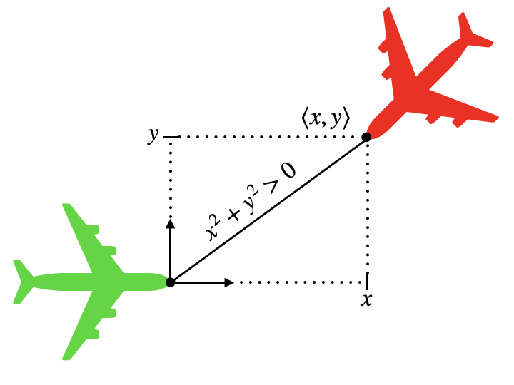
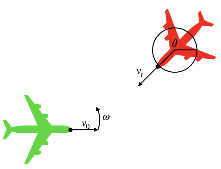
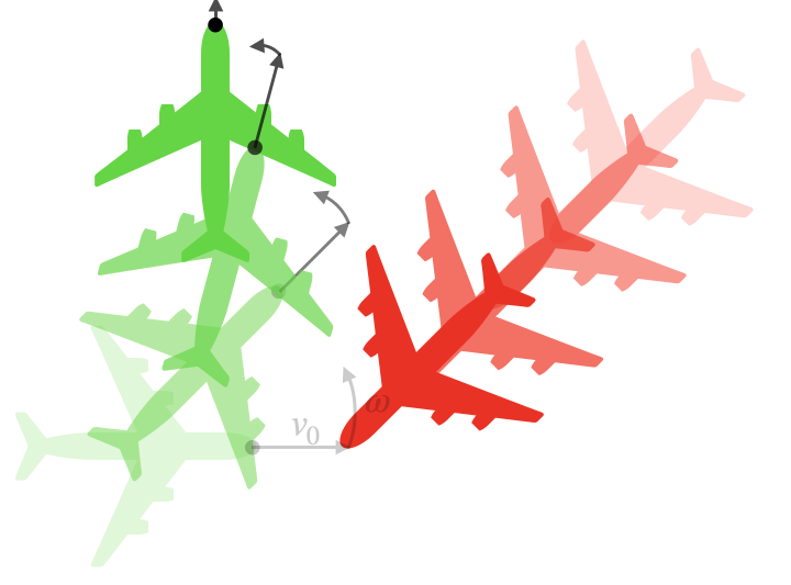
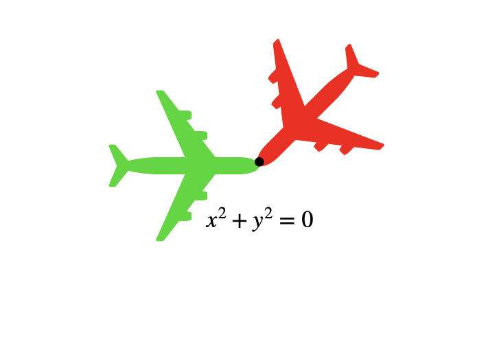
![[Uncaptioned image]](/html/2401.12061/assets/images/proof-state.png)