RUMBoost: Gradient Boosted Random Utility Models

Abstract

This paper introduces the RUMBoost model, a novel discrete choice modelling approach that combines the interpretability and behavioural robustness of Random Utility Models (RUMs) with the generalisation and predictive ability of deep learning methods. We obtain the full functional form of non-linear utility specifications by replacing each linear parameter in the utility functions of a RUM with an ensemble of gradient boosted regression trees. This enables piece-wise constant utility values to be imputed for all alternatives directly from the data for any possible combination of input variables. We introduce additional constraints on the ensembles to ensure three crucial features of the utility specifications: (i) dependency of the utilities of each alternative on only the attributes of that alternative, (ii) monotonicity of marginal utilities, and (iii) an intrinsically interpretable functional form, where the exact response of the model is known throughout the entire input space. Furthermore, we introduce an optimisation-based smoothing technique that replaces the piece-wise constant utility values of alternative attributes with monotonic piece-wise cubic splines to identify non-linear parameters with defined gradient. We demonstrate the potential of the RUMBoost model compared to various ML and Random Utility benchmark models for revealed preference mode choice data from London. The results highlight both the great predictive performance and the direct interpretability of our proposed approach. Furthermore, by analysing the non-linear utility functions, we can identify complex behaviours associated with different transportation modes which would not have been possible with conventional approaches. The smoothed attribute utility functions allow for the calculation of various behavioural indicators such as the Value of Time (VoT) and marginal utilities. Finally, we demonstrate the flexibility of our methodology by showing how the RUMBoost model can be extended to complex model specifications, including attribute interactions, correlation within alternative error terms (Nested Logit model) and heterogeneity within the population (Mixed Logit model).

[inst1]organization=Department of Civil, Environmental and Geomatic Engineering, University College London,addressline=Gower Street, city=London, postcode=WC1E 6BT, country=United Kingdom

1 Introduction and literature review

Discrete choice models (DCMs), based on Random Utility theory, have been used extensively to model choices over the last 50 years (Ben-Akiva and Lerman, 1985; Train, 2009), including the choice of travel mode. DCMs have many desirable qualities: most crucially, their parametric form is directly interpretable and allows for the integration of expert knowledge consistent with behavioural theory. For example, with a DCM, it is possible to: (i) ensure marginal utilities in the model are monotonic (e.g. that increasing the cost of an alternative will always decrease its utility); (ii) restrict the utilities of each alternative to be dependent only on the attributes (or features) of that alternative; and (iii) define arbitrary interactions of socio-economic characteristics and alternative-specific attributes. These three points are essential to derive key behavioural indicators, such as elasticities and Value of Time (VoT), used to inform transport policies and investment decisions. However, the parametric form of DCMs is not without disadvantages. Crucially, the linear-in-parameters utility functions are relatively inflexible and must be specified in advance by the modeller. As such, these models may fail to capture complex phenomena and non-linear effects in human behaviour. Among DCMs, one of the best-known and most widely used models is the Multinomial Logit model (MNL) derived by McFadden et al. (1973). The model assumes that the error term is a type 1 extreme value (EV) random variable, which is independent and identically distributed (i.i.d.) across all alternatives and observations. This formulation results in a closed-form expression of the probability, allowing for easier estimation of the model parameters. However, more complex model specifications exist, for example to capture: (i) different distributions of the error term; (ii) nesting (joint consideration) of alternatives; (iii) behavioural heterogeneity across individuals in the population; and (iv) behavioural heterogeneity across sequential choices.

There have been numerous attempts to apply machine learning (ML) probabilistic classification algorithms, such as neural networks and ensemble learning, to investigate choice behaviour. These models exhibit high predictive performance and, thanks to their data-driven nature, do not require any utility functions to be specified in advance of model estimation. However, they lack an underlying behavioural model and so it is not possible to guarantee consistency of forecasts or derive behavioural indicators such as Value of Time (VoT) or willingness-to- pay from the model parameters. Initial approaches for analysing these models from a behavioural perspective rely on approximating the partial derivatives of the output probabilities of unconstrained ML classifiers in order to define elasticities (and therefore marginal rates of substitution/VoT) for variables of interest. Wang et al. (2020) use this approach to extract economic indicators from neural networks for mode choice problems, whilst Ángel Martín-Baos et al. (2023) extend this to several other classification algorithms, including Gradient Boosting Decision Trees, the Random Forest, and Support Vector Machines. Unlike marginal utilities from a DCM, which have a parametric functional form, the probability derivatives of ML classifiers provide only a numeric estimate of the point elasticities at observed data points. Furthermore, as the underlying models are unconstrained, they exhibit several qualities that are inconsistent with random utility theory, including: (i) non-monotonic elasticities, leading to unwanted behaviours, such as a negative VoT; and (ii) including all features for all alternatives uniformly, therefore violating the independence of irrelevant alternatives assumption. As such, these techniques have seen limited real-world use and practitioners continue to rely predominantly on parametric DCMs. That being said, the ability of ML models to capture complex non-linear relationships as well as their improved predictive accuracy makes them an attractive proposition.

In response to these limitations, there has been an emergence of hybrid data-driven utility models in recent years, that attempt to combine the benefits of ML and DCMs. These can largely be grouped into two different approaches:

1. adding additional constraints to machine learning models (e.g. monotonicity, alternative-specific attributes, etc) so that their output can mimic DCM utility values; and

2. using data-driven approaches to automate or assist with identifying suitable parametric utility functions.

There have been several studies which attempt to incorporate key components from DCMs through making appropriate constraints on the structure of ML models. This analysis stems from the fact that probabilistic ML classifiers, such as neural networks and GBDTs, make use of the same logistic function (commonly referred to as softmax in ML) as the MNL to generate choice probabilities over each alternative; replacing the linear-in-parameter utility functions of the MNL with a complex network of neurons with non-linear activation functions (in the case of the neural network) or ensemble of regression trees (in the case of GBDTs). As such, with suitable constraints on the model, the pre-softmax regression values for each alternative can be considered as pseudo-utilities. The most important of these constraints is that the pseudo-utility of each alternative is a function of only the attributes of that alternative (alongside the socio-economic characteristics of the decision-maker), therefore obeying the independence of irrelevant alternatives assumption. Without this assumption, it is not possible to perform a utility-based behavioural analysis as modifying one attribute would affect the utility values of all alternatives. Wang et al. (2021) build on their prior work of modelling choices with DNNs by defining a separate sub-network per alternative, dependent only on the attributes of that alternative, thus allowing for more robust behavioural indicators to be extracted. Similarly, Martín-Baos et al. (2021) make use of kernel Logistic Regression (KLR) (where the non-linearity is achieved through transforming the input data with a kernel) to learn the deterministic part of each alternative utility by having one kernel per alternative. This allows for behavioural indicators to be defined in the pseudo-utility space, rather than the probability space. Other studies instead use a neural network to complement a conventional utility model. Sifringer et al. (2020) use a Convolutional Neural Network (CNN) to learn a linear-in-parameter utility function for the alternative-specific attributes alongside a DNN to get socio-economic interactions, adding them to the pseudo-utility output in a second stage. In a similar approach, Wong and Farooq (2021) use a Residual Neural Network to add a non-linear, fully-connected residual on top of the linear pseudo-utility at each layer of the network.

However, these studies still lack of a key component of the interpretability and extrapolation ability of DCMs: monotonicity of marginal pseudo-utilities. Whilst not relying on traditional deep learning models, there are several studies that allow for monotonicity of marginal utilities in ML models. Kim and Bansal (2023) use a lattice network with input and output calibration layer to account for non-linearities and partial monotonicity. Krueger and Daziano (2022) replace the sum operator in a traditional Mixed Logit model with the Choquet integral, accounting for attribute interaction under monotonicity. Lastly, Aboutaleb (2022) take advantage of the sum of squares of polynomials to learn data-driven utility functions under monotonicity and shape constraints.

Finally, some researchers retain the traditional structure of the utility function but add data-driven components such as learned parameters or assisted utility specification. Han et al. (2022), with the TasteNet model, use a Deep Neural Network to learn individual-specific parameters from socio-economic characteristics, constraining the sign of the parameters with the appropriate activation function. Instead of replacing the deterministic utility by a data driven model, Hillel et al. (2019) and Ortelli et al. (2021) use data-driven models to assist the modeller with utility specification. The first paper suggests potential non-linear interactions of attributes from the gain of split points in a GBDT algorithm. The second study proposes an algorithm for automatically evaluating multiple model specifications by drawing the Pareto frontier, which is useful in assessing the quality of model specification under multiple objectives. However, the modeller still needs to pre-specify the input space and identify non-linearities.

The summary of state-of-the-art practices in hybrid utility models is in Table 1. The features that we consider in the table are if the models: (i) include alternative-specific attributes; (ii) incorporate monotonicity constraints; (iii) have intrinsically interpretable pseudo-utilities, as in DCMs; (iv) provide automatic identification of non-linearity in the pseudo-utilities, i.e the complete non-linear transformations from the input variable to the pseudo-utilities are observable; and (v) include non-i.i.d. error terms, therefore allowing for complex model specifications such as the Nested Logit or the Mixed Logit models; In this paper, we provide an algorithm to directly learn the non-linear full functional form of the utility, while ensuring alternative-specific attributes and monotonicity on key attributes.

Table 1: Summary of state-of-the-art practice in hybrid utility models. A cross (X) means that the model implements the feature and a tilde ($\sim$) means that the model partly incorporates the feature. Complete explanations on the features that we consider for each column are in the text.

Papers	Alternative specific attributes	Monotonicity constraint	Intrinsically interpretable utility function	Automatic idenfication of non-linearities	Non-i.i.d error terms
Wang et al. (2021)	X
Martín-Baos et al. (2021)	X
Wong and Farooq (2021)	X		$\sim$		X
Sifringer et al. (2020)	X		$\sim$		X
Han et al. (2022)	X	X	X
Kim and Bansal (2023)	X	X	$\sim$	$\sim$
Krueger and Daziano (2022)	X	X	$\sim$		X
Aboutaleb (2022)	X	X	X		X
Ortelli et al. (2021)	X	X	X		X

Whilst the above review evaluates the literature in hybrid data-driven utility modelling, it is also worth considering the more general field of eXplainable Artificial Intelligence (XAI), where researchers aim to add explanations to the predictions of general purpose ML algorithms. The most well known XAI techniques, in use across multiple fields, are: LIME (Ribeiro et al., 2016) and SHAP (Lundberg and Lee, 2017). Several researchers use them to provide interpretability of ML classifiers in a mode choice context (Tamim Kashifi et al., 2022; Ren et al., 2023; Dahmen et al., 2023; Ángel Martín-Baos et al., 2023). However these methods are local approximations of the model relying on data points and, therefore, have no guarantee of validity outside of the input space. On the other hand, Explainable Boosting Machine (EBM) from Caruana et al. (2015) is an example of interpretable Gradient Boosting Decision Trees algorithm. They achieve interpretability by growing shallow regression trees. However, the model does not allow the modeller to specify alternative-specific variables and monotonicity is only applied as a post-processing tool on features without interaction. In addition, a feature can interact with several other features simultaneously, which is inconsistent with random utility theory. We also observe that the majority of research on ML models for choice modelling focuses on neural networks. Although neural networks have numerous applications in many fields and show great results, other algorithms exhibit better performance on classification tasks such as choice modelling. In particular, GBDT models, including XGBoost (Chen and Guestrin, 2016) and LightGBM (Ke et al., 2017) have demonstrated state-of-the-art predictive performance for a variety of classification tasks (Hillel et al., 2018; Ángel Martín-Baos et al., 2023). These models, despite lacking of behaviour interpretability, consistency and robustness (like other ML models) show great interpretability potential due to their additive nature. Furthermore, existing ML approaches have continued to rely on the logit formulation, with i.i.d. EV error terms. As such, they cannot capture complex behavioural phenomenons (e.g. panel effects, dynamic or sequential choice situations, nesting of alternatives, etc).

In this paper, we present Random Utility Models with Boosting (RUMBoost) which aims to combine the predictive power of GBDTs with the interpretability and behavioural consistency of DCMs. At a high level, RUMBoost replaces each parameter in the utility specifications of traditional DCMs with an ensemble of regression trees, allowing for non-linear parameters to be extracted directly from data. Algorithmically, RUMBoost consists of two parts: (i) Gradient Boosted Utility Values(GBUV), where ensembles of regression trees are used to impute piece-wise constant values for each parameter in each pseudo-utility specification; and (ii) Piece-wise Cubic Utility Functions(PCUF), where monotonic piece-wise cubic splines are optimised to fit the GBUV outputs, to allow for a defined gradient for each parameter where elasticities are needed.

The GBUV output effectively defines piece-wise constant pseudo-utility specifications that are consistent with a DCM, with the ability to constrain the model to have: (i) pseudo-utility functions depending only on their alternative-specific attributes and socio-economic characteristics; (ii) monotonicity of marginal pseudo-utilities; and (iii) arbitrary interactions between variables as defined by the modeller. Furthermore, the GBUV output is intrinsically interpretable, with the exact functional form observable to the modeller over the full input space of each variable. Hereafter, we no longer distinguish between utility and pseudo-utility as we believe that, with the constraints aforementionned, the GBUV output can be interpreted as utility values.

As the GBUV output is piece-wise constant, it does not have a defined gradient, with the gradient being either zero or infinite at any given point. As such, behavioural indicators such as elasticities and VoT cannot be extracted directly. This is addressed through the second element of RUMBoost, PCUF. PCUF only needs to be applied for variables for which elasticities are needed (typically the alternative-specific attributes), which optimises a set of piece-wise cubic splines (polynomials) to obtain a defined gradient over the full range of the input space. This allows the modeller to compute behavioural indicators such as the Value of Time (VoT).

The flexibility of our approach allows for estimating complex model structures with correlated error terms such as the Nested Logit model or accounting for population heterogeneity such as the Mixed Logit model. The model is implemented with Python and the code is freely available on GitHub (https://github.com/NicoSlvd/RUMBoost).

The rest of the paper is organised as follows: Section 2 presents the methodology of this paper, the results of a case study are presented in Section 3, Section 4 provides some model extensions, and Section 5 concludes and suggests areas of improvement for future work.

2 Methodology

2.1 Theoretical background

We summarise here key theory of both RUMs and GBDTs under a unified notation in order to help the reader understand our approach. For a more detailed background on each approach, we direct the reader to the following texts: Ben-Akiva and Lerman (1985); Train (2009); Friedman (2001); Chen and Guestrin (2016); Ke et al. (2017).

2.1.1 RUMs

Discrete Choice Models based on Random Utility theory assume that individuals choose the alternative that maximises their utility, a latent measure of the attractivity of an alternative. The utility is usually defined as follows:

$$U_{in}=V_{in}+\varepsilon_{in}$$ (1)

where $V_{in}$ is the observable utility and $\varepsilon_{in}$ the error term capturing unobserved variables for alternative $i$ and individual $n$. In a DCM, $V_{in}$ is a manually specified linear-in-parameters function of the variables, such that:

$$V_{in}=\beta_{i,0}+\sum_{k}^{K}\beta_{i,k}x_{ikn}$$ (2)

where $K+1$ parameters associated with $K$ variables $x_{ikn}$ have to be estimated from the data. For simplicity, we consider here the MNL model, where the error term is assumed to be i.i.d, following an extreme value distribution of type 1 (Gumbel). We will later demonstrate more complex model specifications where the error terms are allowed to be correlated across alternatives. For the MNL, in a classification problem with $J$ classes, the probabilities are given by the multi-class logistic function:

$$P_{in}=\frac{e^{V_{in}}}{\sum_{j}^{J}e^{V_{jn}}}$$ (3)

The qualities of the MNL model are directly derived from the parametric form of $V_{in}$. In particular, it is intrinsically interpretable because there are no variable interactions.

In addition, the modeller can easily incorporate domain knowledge through alternative-specific attributes and monotonicity of marginal utilities. For a multi-class classification problem with $J$ classes, and $K$ explanatory variables, we define:

$$\bm{x}_{i}=\bm{a}_{i}\cup s$$ (4)

where $x_{i}$ is the set of variables for alternative $i$ and

1. $|\bm{x}_{i}|\leq K$, i.e. the cardinality of $\bm{x}_{i}$ should be smaller or equal than the number of attributes $K$

2. $\bm{a}_{i}$ is the set of alternative-specific attributes for alternative $i$, such that $\bm{a}_{i}\in\bm{x},\ \forall i$ and $\bm{a}_{i}\cap\bm{a}_{j}=\emptyset,\ \forall i\neq j$

3. $\bm{s}$ is the set of socio-economic characteristics such that $\bm{s}\in\bm{x}$ and $\bm{s}\cap\bm{a}_{i}=\emptyset,\ \forall i$

Discrete choice models also guarantee the monotonicity of marginal utilities. A positive (resp. negative) monotonic relationship implies that an increasing attribute $\bm{x}_{k}$ will increase (resp. decrease) the value of the utility function $V_{in}$. The signs of parameters in DCMs allow the modeller to easily verify the monotonicity of an attribute and, if needed, to constrain it with parameter bounds.

Finally, the gradient is always defined and easy to compute, which allows for the derivation of behavioural indicators. Among them, the Value of Time (VoT) is an important measure of the perceived cost of travelling time by individuals. The VoT of an alternative $i$ is defined as follows:

$$VoT_{i}=\frac{\partial V_{i}}{\partial x_{i,time}}\cdot\frac{1}{\frac{\partial V_{i}}{\partial x_{i,cost}}}=\frac{\beta_{i,time}}{\beta_{i,cost}}$$ (5)

where $\beta_{i,time}$ and $\beta_{i,cost}$ are the parameters associated with the time $x_{i,time}$ and cost $x_{i,cost}$ attributes of the utility function $V_{i}$.

2.1.2 Gradient boosting

The following notation combines that of Friedman (2001) and Chen and Guestrin (2016), summarising the GBDT algorithm commonly used in popular libraries such as XGBoost and LightGBM. Deep learning models, including DNNs and GBDT use the same multi-class logistic function (typically referred to as the softmax function) as the MNL, which means that they are based on the same assumptions on the error term. In other words, these models first estimate a latent regression value for each class which is then used to generate choice probabilities. The advantage of these models over a linear-in-parameter RUM is that they are inherently non-linear, and so can capture complex relationships between the input features and the choice probabilities. However, unlike in RUMs, these regression models: (i) are a function of all explanatory variables/features (i.e. attributes of each alternative); (ii) do not contain any constraints to represent behavioural assumptions; (iii) allow for complex feature interactions that cannot be constrained (or in many cases even observed) by the modeller; and (iv) have an unknown functional form that is not observable by the modeller. Formally, the ML predictive function $F_{i}(\textbf{x})$ is used to replace the deterministic part of the utility function $V_{i}(\textbf{x})$. In GBDT algorithms, the predictive function is an additive function of the form:

$$V_{i}(\textbf{x})=F_{i,m}(\textbf{x})=\sum_{m}f_{i,m}(\textbf{x})$$ (6)

where $f_{i,m}(\textbf{x})$ is the output of a single regression tree. At each boosting round $m$, assuming $J$ classes, $J$ regression trees are induced to directly minimise the following objective:

$$L=\sum_{n=1}^{N}\sum_{i=1}^{J}\ell(y_{in},\hat{y}_{in,m-1}+f_{i,m}(\bm{x}_{in}))$$ (7)

where:

• $N$ is the number of observations in the dataset;

• $y_{in}=1$ if the choice $i_{n}$ of the individual $n$ is $i$, and $0$ otherwise; and

• $\hat{y}_{in,m-1}$ is the predicted probability of class $i$ and observation $n$ with attributes $\bm{x}_{in}$ at iteration $m-1$, i.e. $\hat{y}_{in,m-1}=F_{i,m-1}(x_{in})$.

This optimisation problem has no closed-form solution. It is generally solved by taking the Taylor second-order approximation of the loss function:

$$L=\sum_{n=1}^{N}\sum_{i=1}^{J}\ell(y_{in},\hat{y}_{in,m-1})+g_{in}f_{i,m}(\bm{x}_{in})+\frac{1}{2}h_{in}f_{i,m}(\bm{x}_{in})^{2}$$ (8)

where $g_{in}=\partial\ell(y_{in},\hat{y}_{in,m-1})/\partial\hat{y}_{in,m-1}$ and $h_{in}=\partial^{2}\ell(y_{in},\hat{y}_{in,m-1})/\partial^{2}\hat{y}_{in,m-1}$ are the first and second derivative of the loss function with respect to the prediction for observation $n$ and class $i$. Here, the Hessian matrix is replaced by a diagonal approximation following Friedman (2001), which means that each class prediction is assumed to be independent. This approximation is crucial for computational efficiency and allows for efficient optimisation of the loss function. In addition, we can ignore the constant term $\ell(y_{in},\hat{y}_{in,m-1})$ for the minimisation task.

Assuming that we have $L$ terminal nodes (i.e. the bottom nodes of the regression tree) resulting in $L$ regions $L_{im}$ for a tree of class $i$ at iteration $m$, each observation will belong uniquely to one of the region $L_{im}$, such that Equation 8 becomes:

$$L=\sum_{i=1}^{J}\sum_{l\in L_{im}}(\sum_{n\in l}g_{in})\gamma_{l,im}+\frac{1}{2}(\sum_{n\in l}h_{in})\gamma_{l,im}^{2}$$ (9)

with $\gamma_{l,im}$ being the leaf value at region $l$ for class $i$. Therefore, by taking the first derivative with respect to $\gamma$ and setting it to $0$, we obtain the optimal leaf value:

$$\gamma_{l,im}=-\frac{(\sum_{n\in l}g_{in})}{(\sum_{n\in l}h_{in})}$$ (10)

By substituting Equation 10 into 9, and assuming a split point that would lead to a left $L_{left,im}$ and right $L_{right,im}$ regions, we obtain the loss reduction for splitting:

$$L_{split}=\frac{1}{2}\sum_{i=1}^{J}\left(\sum_{l_{left}\in L_{left,im}}\frac{(\sum_{n\in l_{left}}g_{in})^{2}}{\sum_{n\in l_{left}}h_{in}}+\sum_{l_{right}\in L_{right,im}}\frac{(\sum_{n\in l_{right}}g_{in})^{2}}{\sum_{n\in l_{right}}h_{in}}-\sum_{l\in L_{im}}\frac{(\sum_{n\in l}g_{in})^{2}}{\sum_{n\in l}h_{in}}\right)$$ (11)

Therefore, we can choose the split point that maximises the loss reduction. For a classification problem, the loss function is usually defined as:

$$\ell=y_{in}\cdot\log(p_{i}(\bm{x_{in}})),$$ (12)

where $p_{i}(\bm{x}_{in})=\hat{y}_{in}$. This equation is typically referred to as the cross-entropy loss in ML contexts, though is equivalent to the log likelihood in RUMs. As in the MNL, we can obtain the predicted probabilities of each class using the softmax function:

$$p_{i}(\bm{x}_{in})=\frac{e^{V_{i}(\bm{x}_{in})}}{\sum_{j=1}^{J}e^{V_{j}(\bm{x}_{jn})}},$$ (13)

Plugging Equations 12 and 13 into Equation 10 gives:

$$\gamma_{l,im}=\frac{J-1}{J}\frac{\sum_{\bm{x}_{in}\in R_{l,im}}y_{in}-p_{i}(\bm{x}_{in})}{\sum_{\bm{x}_{in}\in R_{l,im}}p_{i}(\bm{x}_{in})(y_{in}-p_{i}(\bm{x}_{in}))}$$ (14)

where $\frac{J-1}{J}$ is a factor accounting for redundancy.

The utilities of each ensemble for each individual can then be updated at each iteration:

$$V_{i,m}(x_{in})=V_{i,m-1}(\bm{x}_{in})+\sum_{l=1}^{L}\gamma_{l,im}\cdot\mathbf{1}(\bm{x}_{in}\in L_{im})$$ (15)

where $\mathbf{1}(\cdot)$ is the indicator function, i.e. equals $1$ if the argument is true, $0$ otherwise.

Monotonicity is easily implemented in regression trees. If we assume a positive (resp. negative) monotonic relationship for an explanatory variable, a split point that partitions the data in two such that $\mathbf{x}_{left}<\mathbf{x}_{right}$ is only considered if:

$$\gamma_{left}<\gamma_{right}\ \ \ \ \text{(resp.}\ \gamma_{left}>\gamma_{right}\text{)}$$ (16)

Note that, in order to satisfy the monotonicity over the full tree, the subsequent left and right leaf values are bounded by $\frac{(\gamma_{left}+\gamma_{right})}{2}$. The side of the tree and the nature (positive or negative) of the constraint determine if it is a lower or upper bound.

2.2 The RUMBoost model

We first explain here how we adapt the general GBDT model to output Gradient Boosted Utility Values (GBUV) to emulate parametric RUMs. We then present the Piecewise-Cubic Utility Functions (PCUF) algorithm, that outputs smoothed monotonic non-linear parameters.

2.2.1 Gradient Boosted Utility Values (GBUV)

In RUMBoost-GBUV, we replace each parameter in the utility functions of a RUM with an ensemble of regression trees, where the leaves in the regression trees represent the partial utility contribution for the corresponding value of that variable. These can then be added over each tree in the ensemble to find the contribution of each variable to the utility. The overall utility for each alternative can therefore be found by summing the ensembles for each variable over all variables in the utility function. For K parameters applied to K variables, we have:

$$V_{in}=\text{ASC}_{i}+\sum_{k}^{K_{i}}\sum_{m}^{M_{ik}}f_{imk}(x_{ink})$$ (17)

where $\text{ASC}_{i}$ is an Alternative-Specific Constant for alternative $i$ and $M_{ik}$ is the number of regression trees in the ensemble for parameter $k$ for alternative $i$. In other words, by ordering the split points for each variable in ascending order, and adding leaf values for the appropriate values, we can interpret the sum as raw utility values for each variable. This allows us to impute the full functional form of the ”non-linear parameters” with piece-wise constants. In this form, the utility function is non-linear (and non-continuous) and known over the full input space. Probabilities for each alternative can then be calculated with the appropriate transformation (e.g. softmax/logistic function for the MNL model).

For simplicity of notation, the above formulation shows each parameter being applied to a single variable. However, it is possible to define arbitrary feature interactions by allowing the regression trees in each ensemble to split on multiple variables e.g. for an interaction of two variables $k_{1}$ and $k_{2}$ we would have $\sum_{m}^{M_{ik}}f_{imk}(x_{in{k_{1}}},x_{in{k_{2}}})$. This allows the modeller to specify any desired feature interactions as required.

We modify the standard GBDT boosting algorithm in order to identify optimal RUMBoost-GBUV ensembles for each variable (or combination of variables). For a J-class problem, we introduce J trees at each boosting iteration during model training, one for the utility function of each alternative. At each iteration, the model computes choice probabilities for the previous estimates of the utility functions, derives the gradient and hessian of the log-loss, and uses them for boosting the next set of $J$ trees. Each regression tree is added to the ensemble for a single variable, automatically selected by the algorithm in an exhaustive search (for computational efficiency the search is typically limited to a finite number of possible split points) in order to minimise the loss function.

Once the model has been fully trained, we can extract normalised ASCs. We define the non normalised ASCs as:

$$\text{ASC}^{\prime}_{i}=\sum_{k}^{K_{i}}\sum_{m}^{M_{ik}}f_{imk}(0)$$ (18)

Since in RUM only the difference in utilities matter, one of the ASCs can be normalised to $0$. Assuming that the ASC of the alternative $j$ is normalised, we obtain the following set of ASCs:

$$\text{ASC}_{i}=\text{ASC}^{\prime}_{i}-\text{ASC}^{\prime}_{j},\forall i=1,...,J$$ (19)

We build our algorithm on top of LightGBM (Ke et al., 2017), such that each ensemble is a LightGBM Booster object. Therefore, we can make use of the already implemented monotonicity constraint feature to impose monotonicity on utilities as required.

The RUMBoost-GBUV model training algorithm is described formally in Algorithm 1. Note that the algorithm is independent of the assumption on the error terms. This allows RUMBoost-GBUV to be used to emulate any arbitrary model formulation for which the gradient and Hessian of the loss function is defined, including Nested Logit and Mixed Logit models. Furthermore, as the code has been re-implemented from scratch, any ML regressor that can satisfy the constraints described above can be used in place of GBDT.

Algorithm 1 : RUMBoost-GBUV

$\bm{x_{i}}=\bm{a_{i}}+\bm{s}$,    $\forall i=1,...,J$

Positive monotonic set of attributes $\bm{x}_{i}^{+}\subseteq\bm{x}_{i}$,     $\forall i=1,...,J$

Negative monotonic set of attributes $\bm{x}_{i}^{-}\subseteq\bm{x}_{i}$,     $\forall i=1,...,J$

$\bm{x}_{i}^{+}\cap\bm{x}_{i}^{-}=\emptyset$,     $\forall i=1,...,J$

Specify variables interactions

$V_{in}(\bm{x_{in}})=0$,    $\forall i=1,...,J$

for $m=1$ to $M$ do

     Compute $p_{in}(\bm{x}_{in})$

     for $i=1$ to $J$ do

         Compute the first and second derivatives of the loss function

         Choose the split point that maximises the loss reduction of any variable $k$

         Add the regression tree $f_{imk}(x_{ink})$ to its corresponding ensemble

     end for

end for

2.2.2 Piece-wise Cubic Utility Function (PCUF)

The GBUV ensembles for each parameter in Section 2.2.1 are non-continuous, and so have a gradient of either zero or infinite at any point. However, many behavioural indicators require the utility function to have defined gradient to be computed. Therefore, we interpolate the utility values into a smooth function using piece-wise cubic Hermite splines. Using splines ensure that the underlying cubic polynomials have equal values and derivatives at the knots (i.e. boundary points). Given the number of knots and their positions, only the derivative at each knot needs to be computed, making Hermite splines very attractive for efficient computations. Using the approach introduced by Fritsch and Carlson (1980), it is possible to guarantee monotonic splines, where the gradient is always negative or positive (or zero) as required. The interpolation must satisfy two conflicting objectives: (i) fitting the data as well as possible to maintain good predictive power on out-of-sample data; and (ii) being as smooth as possible to obtain relevant behavioural indicators.

The first objective favours a higher number of knots, while the second aims for a lower number so that the derivative is well defined. A natural objective function to capture the trade-off of both these objectives is the Bayesian Information Criterion (BIC), which takes the following form:

$$BIC=-2N\cdot L+df\cdot\ln(N)$$ (20)

where $L$ is the loss function described in Equation 12, $df$ is the degree of freedom of the model, and $N$ is the number of observations. The first part of the function aims for a better fit of the data, while the second part penalises the model for its complexity.

RUMBoost-PCUF, therefore, has two parameters to tune: (i) the number of knots; and (ii) their positions. Given a sequence of $Q+1$ knots $a_{k}=t_{0,k}<t_{1,k}<...<t_{Q,k}=b_{k}$ for an attribute $k$ where $a_{k}$ and $b_{k}$ are the domain where that attribute is defined, the optimal positions and numbers of knots are determined by the following optimisation problem:

$$\min_{t_{q,k}} -2N\cdot L+df\cdot ln(N)$$ (21)

s.t. $$t_{q+1,k}-t_{q,k}>0 \forall q=0,...,Q,\forall k$$

$$t_{0,k}=a_{k} \forall k$$

$$t_{Q,k}=b_{k} \forall k$$

Given the number of knots, there is an optimal position of knots that minimises the loss function. Therefore, the two hyperparameters can be tuned sequentially: the number of knots is selected first and their optimal positions are found with a constrained optimisation solver afterwards. However, this can be a complex optimisation problem if the number of attributes is high, and it has been shown in the literature that it is acceptable to fix the positions of knots over the range of the attribute (e.g., quantile) and optimise only their numbers (Hastie and Tibshirani, 1990). The RUMBoost-PCUF algorithm is summarised in Algorithm 2.

Algorithm 2 : RUMBoost-PCUF

$\bm{x_{i}}=\bm{a_{i}}+\bm{s}$,    $\forall i=1,...,J$

Gradient boosted utility values $V_{ik}$     $\forall i=1,...,J$, $k=1,...,K$

Number of iterations for hyperparameter search $N_{iter}$

for $n=1$ to $N_{iter}$ do

     for $i=1$ to $J$ do

         for $k=1$ to $K$ do

              if $x_{k}\in\bm{a_{i}}$ then

                  Choose a number of knots $Q_{k}$

                  Define the initial position of knots $t_{q,k}=Q_{k}\text{-quantile}(x_{k},q)$    $\forall q=0,...,Q_{k}$

              end if

         end for

     end for

     Optimise the knots position to minimise the $BIC$

end for

2.3 Code and implementation

We implement the model in Python, making use of the library LightGBM for the utility regression ensembles (Ke et al., 2017). Our implementation creates a regression ensemble for each alternative in which the input attributes (or features) can be specified independently. We set up the logistic/softmax function so that in each round of boosting, the trees (and split points in each tree) are selected to directly minimise the log-loss (cross-entropy loss), therefore emulating maximum likelihood estimation (MLE). Separate ensembles for each parameter are obtained by restricting the possible set of feature interactions in each tree. The code makes use of the existing monotonic constraints functionality to guarantee monotonicity of the marginal utilities as required. We have therefore implemented an interface which allows the modeller to specify:

• which attributes should be included in each utility function

• control attribute interactions

• specify which attributes should have monotonic marginal utilities.

Early stopping is used to determine the appropriate number of trees in each ensemble, with boosting terminated once the log-loss does not improve on out-of-sample data for a given number of iterations (e.g. 100). Furthermore, we have written a script that converts model files from the popular choice modelling software Biogeme (Bierlaire, 2023) to be used directly within RUMBoost, therefore allowing modellers to easily replicate any MNL model in RUMBoost. This conversion works using the utility specification to define alternative-specific attributes and control attribute interactions, and using bounds on the parameters to define monotonic constraint. The code is freely available on Github (https://github.com/NicoSlvd/RUMBoost)

3 Detailed case study

We apply our methodology on a case study, where we benchmark RUMBoost against a MNL model and three ML classifiers: Neural Network (NN), Deep Neural Network (DNN) and LightGBM. These models are re-implemented from Ángel Martín-Baos et al. (2023). In addition, we show the non-linear utility functions and compute behavioural indicators. To ensure a fair comparison, RUMBoost is built using the same model specification as the MNL model.

3.1 Case study specifications

We use the London Passenger Mode Choice (LPMC) (Hillel et al., 2018) dataset for our case study, a publicly available dataset providing details of more than 80000 trips in London, alongside their associated mode choice decisions. It is an augmented version of the London Travel Demand Survey (LTDS) trip diary dataset, to include the travel time and cost of alternatives. The dataset contains observations from 17615 households over a three-year period, and there are four possible alternatives: walking, cycling, public transport and driving. The MNL model, also used to create RUMBoost, is a 62-parameter model with alternative-specific constants (ASC). When estimating the MNL model, we normalise the ASC, the generic attributes and the socio-economic characteristics of the walking alternative to zero. The model specification is summarised in Table 2. Lastly, the RUMBoost and ML models are trained on the first two years of the dataset with a 5-fold cross validation scheme designed in such a way that trips performed by the same household members cannot be in different folds, to avoid data leakage. We include an early stopping criterion of 100 iterations, i.e. we stop the training if the performance on the validation set is not improving during 100 iterations. For the ML classifiers, we also include a hyperparameter search. This search is done with the python library Hyperopt (Bergstra et al., 2013), and the search space and results are summarised in A.

Table 2: Variables used in the LPMC RUMBoost and MNL models. For the MNL estimation, the socio-economic characteristics and generic attributes are normalised to 0 for the walking alternative. Purpose and Fuel type are dummy variables where one category is normalised. The constants are not included in the RUMBoost training, but are reconstructed afterwards, following Equation 19.

	Walking	Cycling	Public Transport	Driving
Alternative-specific attributes
Constant		✓	✓	✓
Travel time	✓	✓	✓	✓
Access time			✓
Transfer time			✓
Waiting time			✓
Num. of PT changes			✓
Cost			✓	✓
Congestion charge				✓
Socio-economic characteristics and generic attributes
Straight-line distance	✓	✓	✓	✓
Starting time	✓	✓	✓	✓
Day of the week	✓	✓	✓	✓
Gender	✓	✓	✓	✓
Age	✓	✓	✓	✓
Driving license	✓	✓	✓	✓
Car ownership	✓	✓	✓	✓
Purpose: home-based work	✓	✓	✓	✓
Purpose: home-based education	✓	✓	✓	✓
Purpose: home-based other	✓	✓	✓	✓
Purpose: employers business	✓	✓	✓	✓
Purpose: non-home-based other	✓	✓	✓	✓
Fuel type: diesel	✓	✓	✓	✓
Fuel type: hybrid	✓	✓	✓	✓
Fuel type: petrol	✓	✓	✓	✓
Fuel type: average	✓	✓	✓	✓

3.2 RUMBoost model specification

The MNL model is directly used to specify the constraints of the RUMBoost model. The alternative-specific attributes constraint is directly satisfied by the MNL utility specification. Interactions between attributes are restricted, such that each tree corresponds to a single parameter. Finally, monotonicity constraints are obtained from the bounds that would be applied to the MNL beta parameters (see Table 3), and so applied negatively on travel time, headway, cost and distance, and positively on car ownership and driving license (when applicable).

Table 3: Attributes constrained to monotonicity. Travel time, cost and distance are monotonic negative, i.e. an increase of these attributes will decrease the utility function value. Car ownership and driving license are positive monotonic and applied only on for the driving alternative.

Monotonic negative	Travel time, cost, distance
Monotonic positive	Car ownership*, driving license*
	*Only for the driving alternative

One big advantage of RUMBoost over the more flexible GBDT model is that the additional constraints help to regularise the model and therefore has a lower propensity to overfit compared to the unconstrained GBDT model. We find that the modelling results are less dependent on hyperparameter values, including regularisation parameters. Thus, we use the LightGBM default parameters except for the learning rate, the maximum depth of trees and the number of trees. The number of boosting rounds is obtained with the cross-validation early stopping criterion, where we average the best number of trees of each fold to obtain the final number of trees. As such, we make use of the following parameters for each regression ensemble:

• learning rate: 0.1

• max depth: 1 (following attribute interaction constraints)

• minimum data and sum of hessian in leaf: 20 (default) and 0.001 (default)

• maximum number of bins and minimum of data in bins: 255 (default) and 3 (default)

• monotone constraint method: advanced

• number of boosting rounds (trees): 1300

3.3 Comparisons with other ML models and MNL

The results of the RUMBoost model are benchmarked against the MNL and ML models presented in Section 3.1. We compare the models with their cross-entropy loss (CLE) on the test set (lower is better) and their computational time per cross-validation iteration. The results are shown in Table 4.

Table 4: Benchmark of Classification on LPMC Dataset. The models are compared with their CEL (negative Cross-Entropy Loss, lower the better) on the test set and their computational time for one CV iteration. The training results of RUMBoost-PCUF are the results of the optimisation problem described in Section 2.2.2.

Models	Metrics	LPMC
		5 fold CV	Holdout test set
MNL	CEL	0.6913	0.7085
	Comp. Time [s]	242.14	-
NN	CEL	0.6516	0.6667
	Comp. Time [s]	7.85	-
DNN	CEL	0.6613	0.6735
	Comp. Time [s]	3.89	-
LightGBM	CEL	0.6381	0.6537
	Comp. Time [s]	4.64	-
RUMBoost-GBUV	CEL	0.6570	0.6737
	Comp. Time [s]	6.48	-
RUMBoost-PCUF	CEL	0.6479*	0.6730
	Comp. Time [s]	712.48*	-
			*Not with CV

Overall, the RUMBoost model outperforms the MNL model on both training and testing validations, whilst still ensuring a directly interpretable functional form. Whilst there is a marginal performance sacrifice of the RUMBoost models compared to the unconstrained GBDT and NN models, it is important to note that the functional form of the RUMBoost utilities is directly interpretable over the full input space, allowing for guarantees of behavioural consistency of forecasts, and in the case of RUMBoost-PCUF, extraction of behavioural indicators, which is not possible for the GBDT and NN models. Note that further enhancements of the RUMBoost model, including the functional effects model (see Section 4.3) further narrow this gap. Interestingly, the loss of information due to smoothing is minimal, and the CE loss even improves on the LPMC dataset, even with an objective function penalising complex models. Therefore, we deduce that the piece-wise splines act as further regularisation of the RUMBoost model when there is a sufficient amount of data and splitting points. Computationally, the GBUV algorithm shows similar results than the ML classifiers, which is much better than the MNL model. The PCUF algorithm on the other hand has a big computational time, illustrating the complexity of the optimisation problem.

3.4 Gradient boosted utility values

The primary advantage of using RUMBoost over other unconstrained ML algorithms is that non-linear utility functions can be observed directly. We have access to the ensemble for each parameter thanks to the custom training function. Therefore, we can delve into each tree of each ensemble to retrieve leaf values and splitting points. More specifically, each split point in a regression tree represents a step in the GBUV output for the corresponding parameter. The utility contribution at point $x$ is the cumulative sum of all corresponding leaf values of the trees in the ensemble. These functions are presented for the travel time, cost, departure time and age parameter in Figures 1(a), 1(b), 2(a) and 2(b).

Figure 1(a) shows the impact of travel times on parameter values for the LPMC dataset, with the public transport alternative including both bus and train travel times. From the graph, it can be noted that the walking and driving time parameters have a convex shape, indicating that the increase in a short trip has a greater influence on the utility function than a longer trip. This contrasts with the two parameter values linked to public transport, where bus travel time has an approximately linear curve, and train travel time impact results in a concave parameter values. Finally, the parameter values of cycling is initially convex, then reaches a plateau between 0.5 and 1 hour of travel time, and decreases rapidly after 1 hour. Figure 1(b) depicts the constant utility contributions of travel cost parameter for driving and PT. Interestingly, both parameter values exhibit a similar behaviour. There is first a sharp decrease representing the disutility of travelling, then a plateau, and a final drop around 2 £.

Figures 2(a) and 2(b) show the constant utility values of the age and departure time parameters for each alternative. Following behavioural theory, there are no monotonicity constraints on these variables, but we still observe that increasing age mainly reduces the utility of walking and cycling, with a mostly convex shape. For public transport, the parameter values is the lowest at older ages, and peaks around the age of 20. Finally, for the driving alternative, the utility is higher with younger and older ages, but the lowest point is at the age of 20. Also note that passengers are included in the driving alternatives, explaining the high values for younger and older individuals. Finally, the departure time utilities are stable during the day. The walking and cycling utilities exhibit a sharp increase around midnight. The public transport utility has a higher value on the morning, corresponding to the morning commuting time. Finally, the driving utility decreases until 7h, and increases until the end of the day after that.

(a) Travel time (LPMC)

(b) Cost (LPMC)

Figure 1: Utility contributions of a) travel time and b) cost on the LPMC dataset, both under a negative monotonic constraint. Each step represents a split point of a regression tree in the corresponding ensemble.

(a) Age (LPMC)

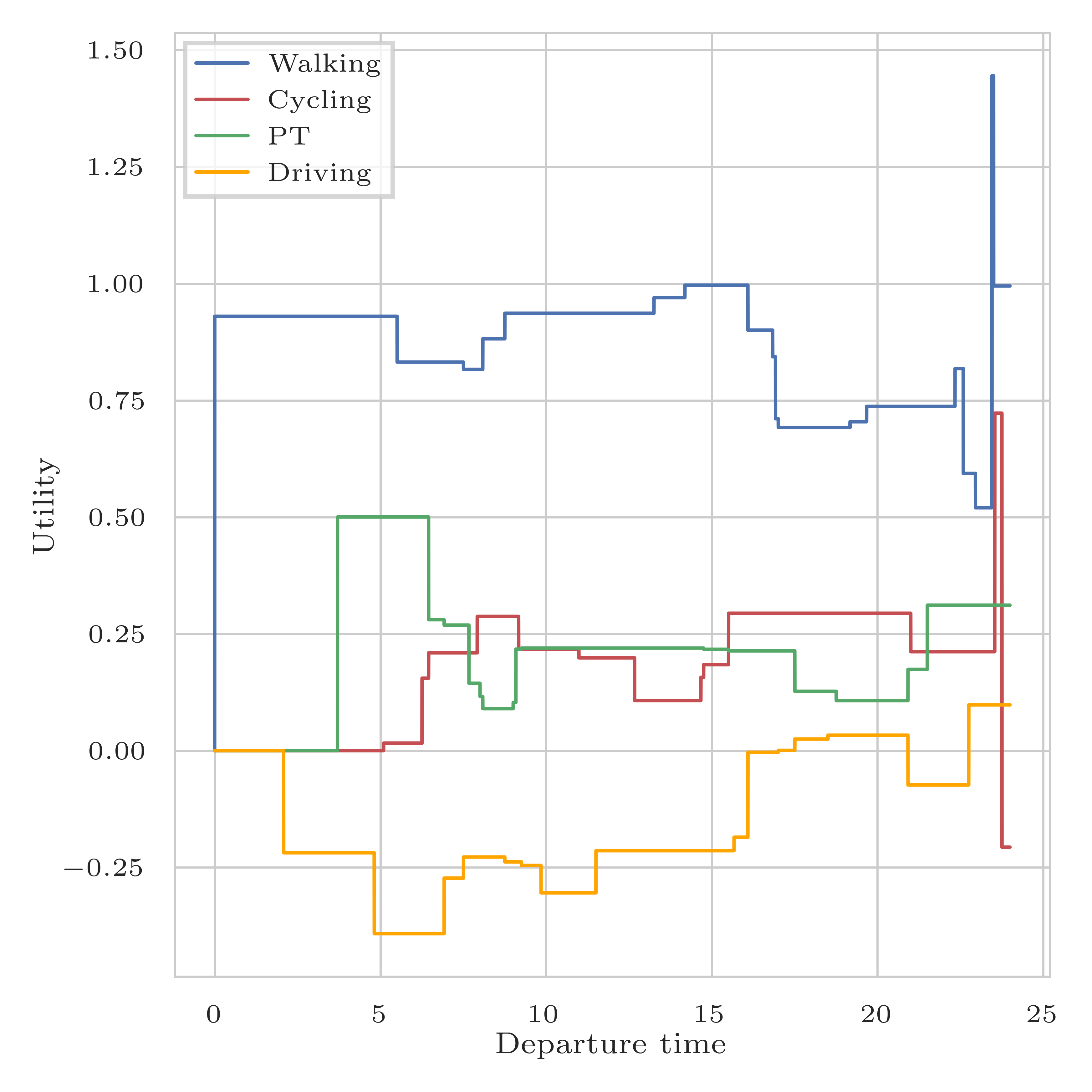
(b) Departure time (LPMC)

Figure 2: Utility contributions of a) age and b) departure time on the LPMC dataset. Both variables are non-monotonic. Each step represents a split point of a regression tree in the corresponding ensemble.

3.4.1 GBUV robustness

To demonstrate the robustness of the GBUV outputs, we perform bootstrap sampling for 100 iterations. We plot the resulting parameter values with their average and show the results for the travel time parameters in Figure 3. To visualise the distribution of the input space, we plot a histogram of the data distribution on top of each figure.

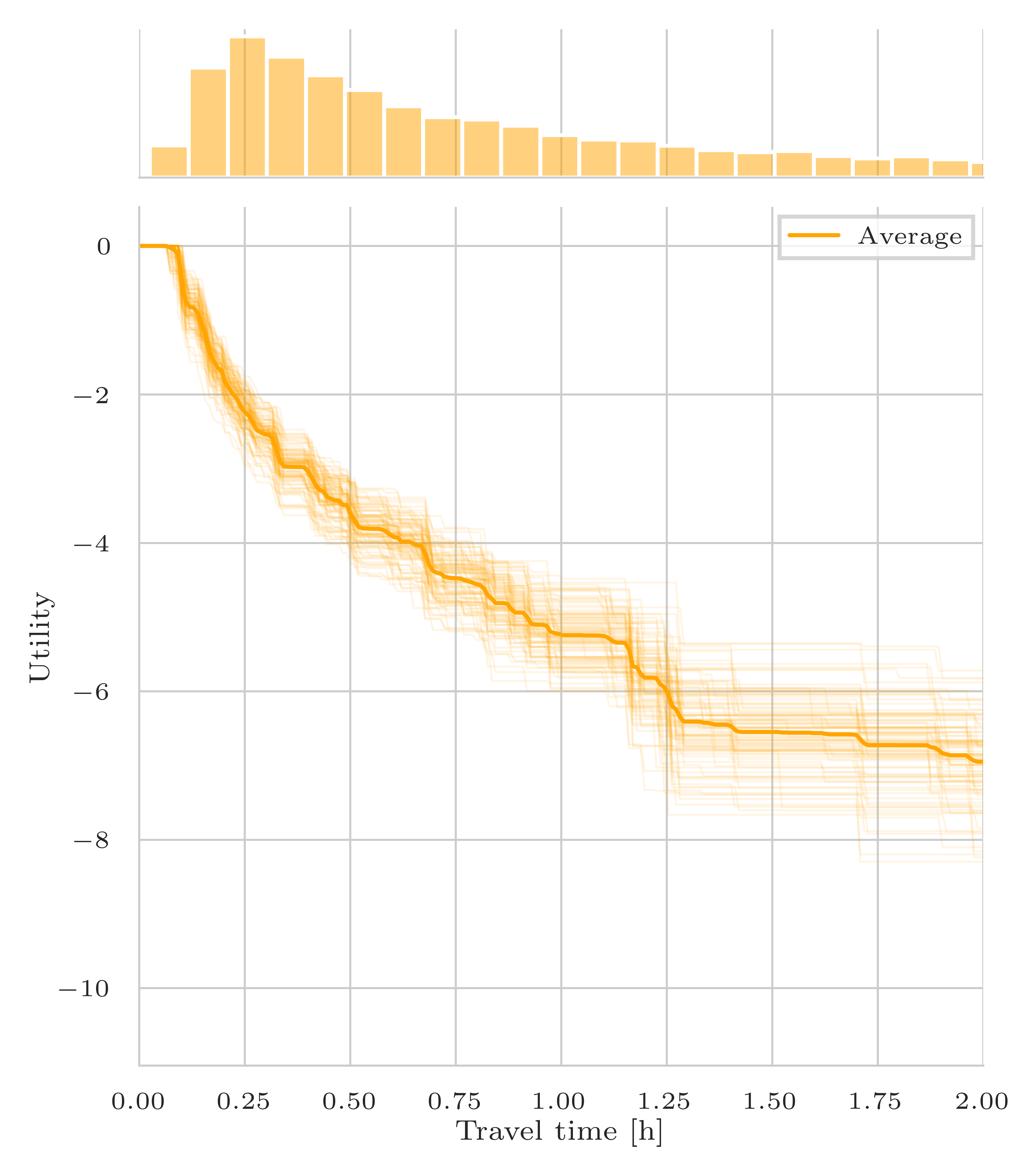
(a) Walking travel time

(b) Cycling travel time

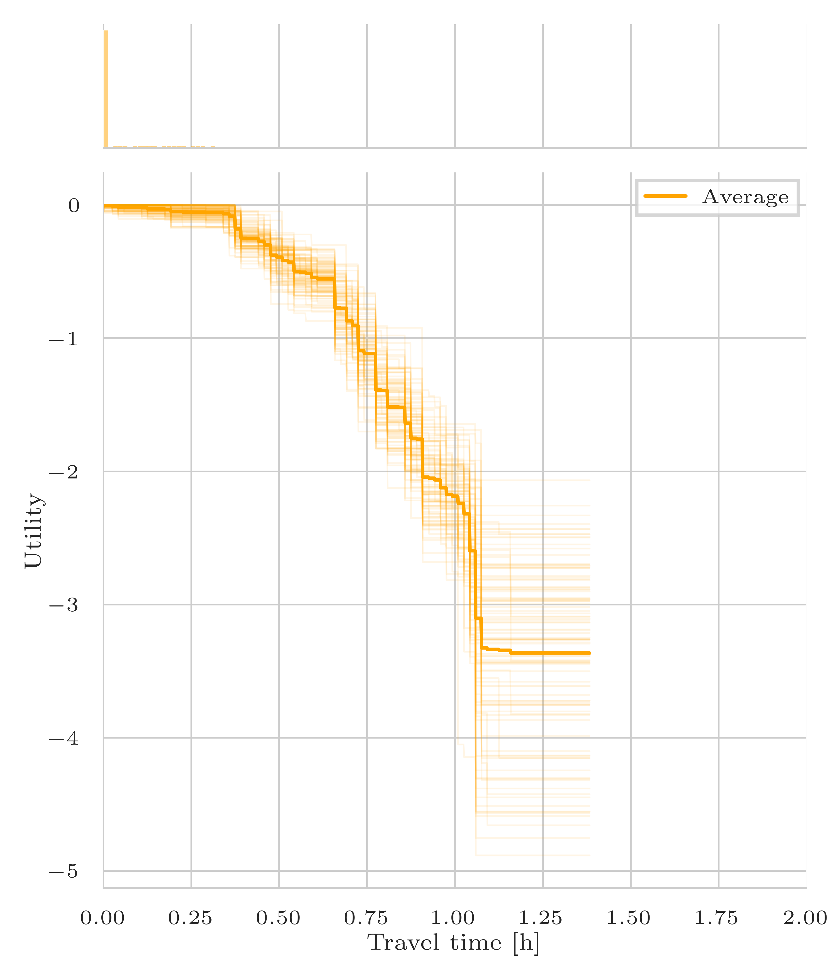
(c) PT - Rail travel time

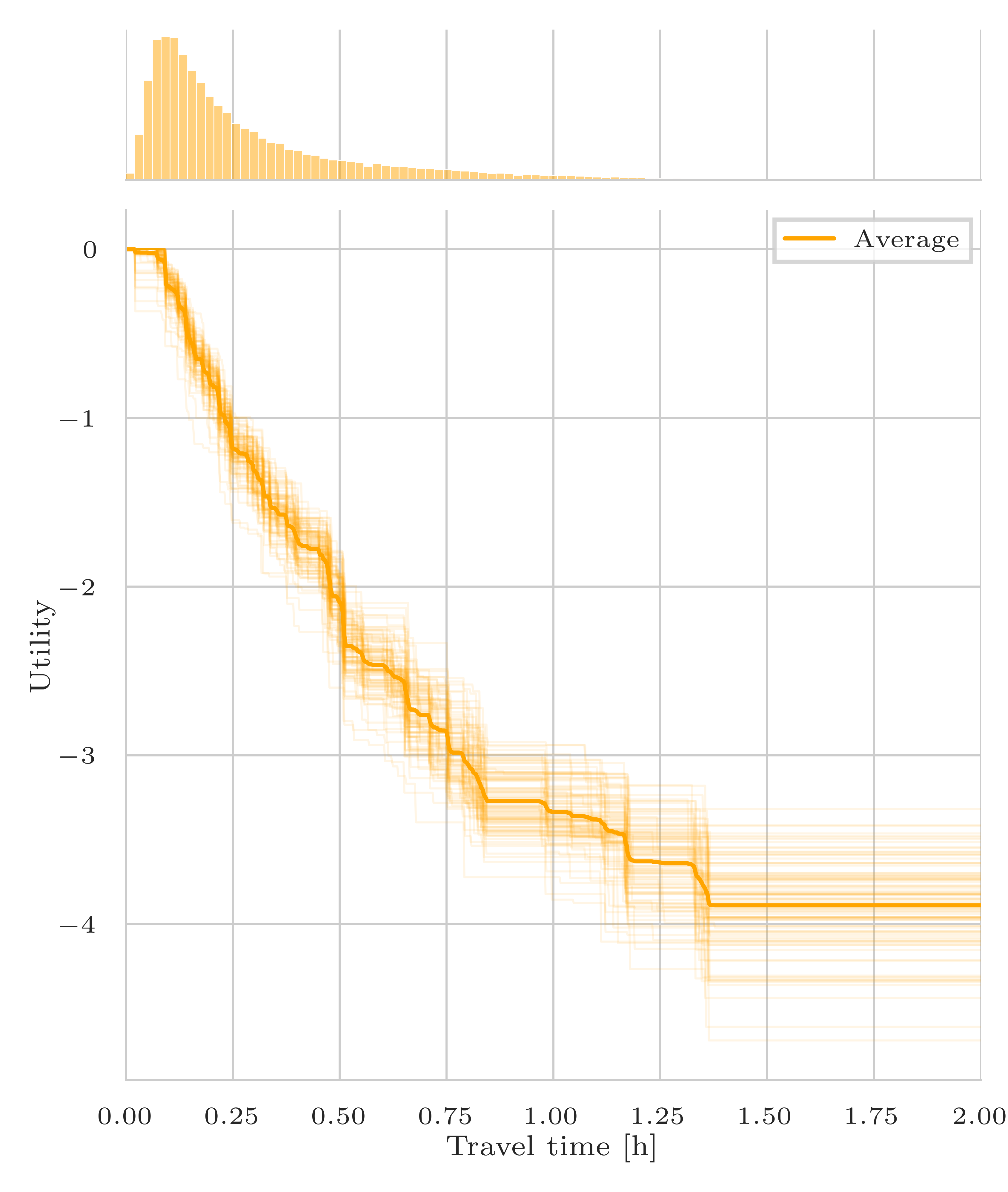
(d) Driving travel time

Figure 3: Utility contributions of the travel time on the LPMC dataset with bootstrapping for a) walking, b) cycling, c) PT and d) driving alternative. Each line with transparency corresponds to a bootstrap sampling iteration. The mean is highlighted, and the distribution of data is shown on top of each figure. The figures are cropped at 2 hours of travel time.

Figure 3 show that, even with sampling with replacement, i.e. changing the distribution of the population, the utility values are robust. While their values may vary slightly, their shape is similar in all utilities, especially when the density of observations is high. The walking and driving travel time (Figures 3(a) and 3(d)) exhibit the best robustness, while cycling travel time (Figure 3(b)) and the rail travel time (Figure 3(c)) are the one showing the most scale variability. However, the cycling alternative is the least chosen alternative, and a high number of individuals have no travel time for the PT alternative, which can explain this finding. These bootstrapped utilities could be further used to calculate confidence interval.

3.5 Piece-wise cubic utility functions

We make use of the SciPy (Virtanen et al., 2020) implementation of monotonic cubic splines (Fritsch and Carlson, 1980; Fritsch and Butland, 1984) to smooth the GBUV outputs to produce piece-wise cubic utility functions. We treat finding the number and location of the knots as a heurisitic optimisation problem where we minimise the BIC of the model likelihood, following the methodology introduced in Section 2.2.2. We make use of the Hyperopt Python library to identify optimal solutions. The case-study model has 15 variables for which we wish to extract marginal utilities. Each search in Hyperopt involves selecting a different number of knots, constrained to be an integer value between a minimum of 3 and up to 8. In total, 25 searches are conducted (i.e. 25 different combinations of numbers of knots for each variable).

The inner optimisation loop then identifies optimal knot locations, given a fixed number of knots for each variable, using the SLSQP (Sequential Least Squares Quadratic Programming) algorithm, implemented in SciPy. We constrain the first and last knots to be at the location of the first and last observations for each variable. For the initial solution for the remaining knots, we follow Wang et al. (2023), where we set the position of $K+1$ knots at the $k/(K+1)^{th}$ quantile.

The optimised number of knots for each variable are shown in Table 5. The use of the BIC as the objective function results in parsimonious solutions, where the number of splines is limited for simple transformations. The straight-line distance is not included for public transport as there were no regression trees in the parameter ensemble. The smoothed PCUF outputs for the travel time and cost parameters are shown in Figure 4. From the graph, it is clear that PCUF output has successfully smoothed the GBUV functions, rather than overfitting with too many splines.

Table 5: Optimal number of knots for PCUF. The number of knots is chosen with a hyperparameter search of 25 iterations

Attributes	Number of knots
Walking
Travel time	6
Distance	6
Cycling
Travel time	6
Distance	6
Public transport
Rail travel time	3
Bus travel time	4
Access travel time	4
Interchange waiting time	8
Interchange walking time	7
Cost	3
Driving
Travel time	5
Distance	4
Cost	3

(a) Travel time

(b) Cost

Figure 4: Piece-wise monotonic cubic spline interpolation of a) travel time and b) cost on the LPMC dataset. The knots are drawn in black and the first and last knots are omitted for clarity. The GBUV used for interpolation are plotted as a scatter plot.

Using the gradients from the PCUF functions, the Value of Time (VoT) can be computed for the alternatives that include both travel time and cost parameters. We define the plot only in the area where the cost derivative is not zero, and we cap the maximum value at 100 £/h and minimum value at 0.1 £/h. We also exclude the flat areas at low and high values of both attributes. As both the travel time and cost attributes are non-linear, the VoT is unique to each combination of travel time and cost. As such, it is represented as a 3D distribution, though note that this distribution is homogeneous across the population. Figure 5 displays the VoT for the PT and driving alternatives on the LPMC dataset on a logarithmic (base 10) scale. We use a logarithmic scale to better visualise the differences among lower VoTs. The value of time of rail (Figure 5(a)) ranges from 2 to 5 £/h for trips lasting less than 0.6 hour and increases to 10 to 20 £/h for travel times of 0.6 to 1 hour. It decreases again after one hour. This suggests that between 0.6 and 1 hour of travel time, individuals are willing to pay more to reduce their travel times. Regarding the value of time for driving (Figure 5(b)), we observe overall a decrease of the travel time with increasing travel time, and an increasing of VoT with increasing cost. The lowest value is around 2 £/h for no cost and 1.3 hours of travel time, and the highest value is capped at 100 £/h for 4£ cost and no travel time. We deduce that individuals with high cost and low travel times are willing to pay more to reduce their travel time.

(a) Rail (LPMC dataset)

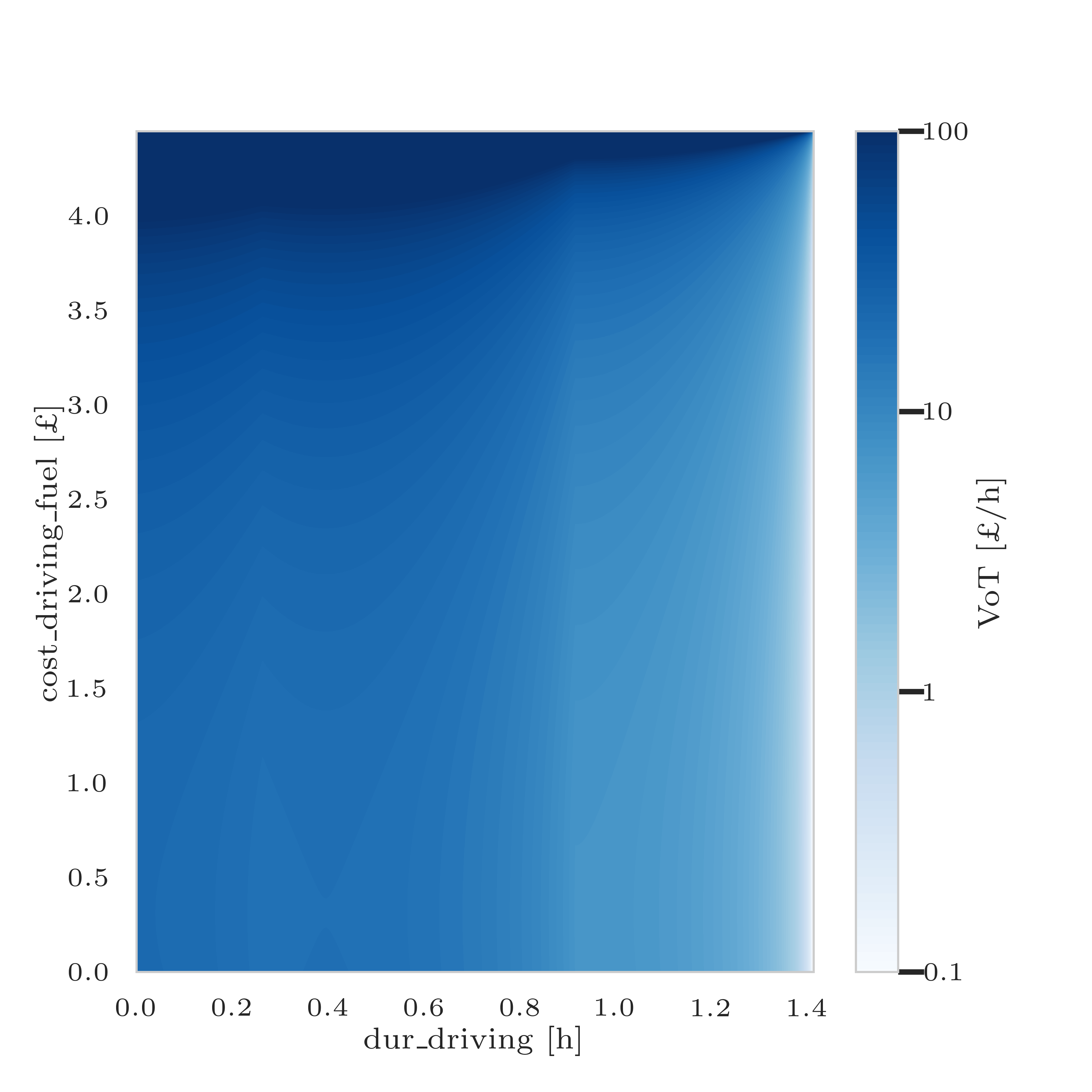
(b) Driving alternative (LPMC dataset)

Figure 5: Value of Time (VoT) for a) rail, b) driving. The VoT is capped at 100£/h, and displayed only where the utility functions derivatives are non zero.

In addition to the contour plot VoT, we also compute the VoT across the population. To do so, we remove observations that have a zero travel time for the rail alternative, and exclude the 0.1% highest values (from 99.9% to 100%). Then, we calculate the VoT of all remaining individuals with their respective costs and travel times. The results are shown in Figure 6. For the PT alternative (Figure 6(a)), the distribution of VoT peaks below 1 £/h and then continuously decreases until 5£/h. For driving VoT (Figure 6(b)), there is a sharp peak at 17.5 £/h. These values are both lower than the VoT extracted from linear-in-parameter RUM models for the same dataset, of 8.73 £/h and 40 £/h respectively (see Hillel (2019), p.133), showing the impact of the non-linear utility specification.

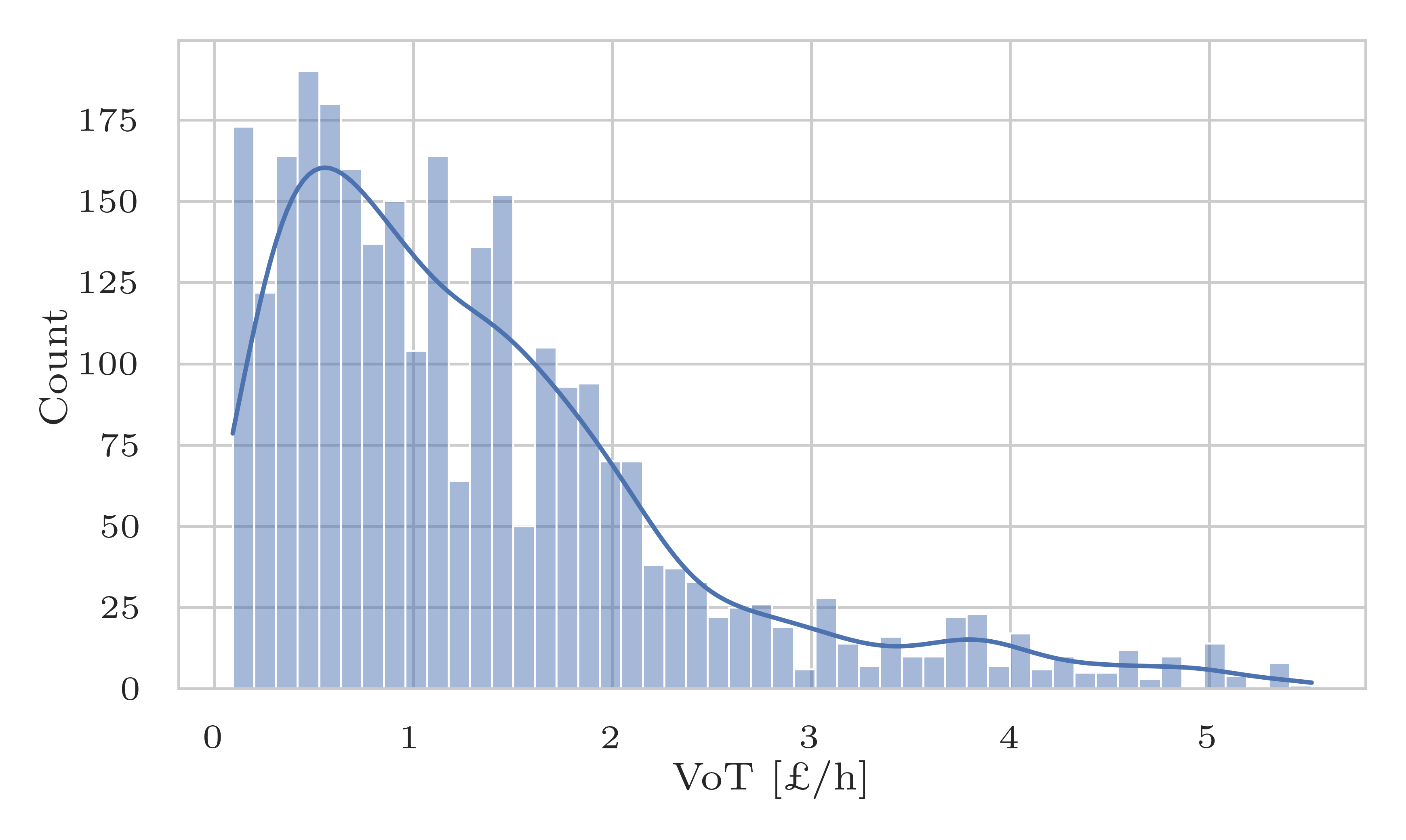
(a) PT alternative

(b) Driving alternative

Figure 6: Histogram of the population Value of Time (VoT) for a) rail, b) driving. The observations with zero travel times, as well as the highest 0.1% VoT values are excluded. The solid line represents the kernel density estimates.

4 Extensions of RUMBoost

In this section, we present three extensions of RUMBoost, highlighting how the approach can be generalised to different modelling scenarios: a) incorporating attribute interactions (Section 4.1); b) assuming alternative correlation within the error term (Section 4.2); and c) accounting for correlation within trips made by the same individual (Section 4.3).

4.1 Second-order attribute interactions

By allowing two continuous attributes to interact, we can consider attribute interactions. In doing so, it is still possible to interpret the ensemble output for these two attributes on a contour plot. As an example, we arbitrarily allow age and travel time to interact. We allow for a max depth of two in each tree to allow for feature interactions and, through early stopping, perform 680 total boosting rounds. Figure 7 shows the resulting contour plot for all alternatives. The contour plots are only monotonic with respect to travel time, as specified in the model. For the walking alternative (Figure 7(a)), longer travel times lead to increased disutility for both younger and older ages, while shorter travel times result in relatively uniform disutility. For cycling (Figure 7(b)), we observe a similar phenomenon for longer travel times but the disutility is still pronounced for older individuals with shorter travel times, which aligns with the expectation that cycling may be less feasible for older individuals. In the case of public transport (Figure 7(c)), disutility is more significant for younger ages and less pronounced for adults and shorter travel times. Lastly, the disutility associated with an increase in age or travel time for the car alternative (Figure 7(d)) remains relatively constant, but it is mitigated for ages below 10 and travel times shorter than 0.5 hour.

(a) Walking alternative

(b) Cycling alternative

(c) Public transport alternative

(d) Driving alternative

Figure 7: Utility function in the form of a contour plot for the travel time (x axis) with age (y axis) interaction on the LPMC dataset for a) walking, b) cycling, c) PT and d) driving alternative. Only the travel time is subject to monotonicity constraint.

4.2 Nested RUMBoost

Until now, we assumed the error terms for each alternative to be distributed i.i.d., leading to the MNL model formulation. We show that we can relax this assumption with our approach by assuming an error term correlated within alternatives. In RUM, this error term leads to the Nested Logit (NL) model. We update the probability formula and update the gradient and hessian (second derivative) computations accordingly, giving:

$$P(i)=P(i|m)P(m)$$ (22)

where the probability of choosing $i$ knowing the nest $m$ is:

$$P(i|m)=\frac{e^{\mu_{m}V_{i}}}{\sum_{j\in m}e^{\mu_{m}V_{j}}},$$ (23)

while the probability to choose the nest $m$ is:

$$P(m)=\frac{e^{\tilde{V}_{m}}}{\sum_{p=1}^{M}e^{\tilde{V}_{p}}},$$ (24)

where:

• $\tilde{V}_{m}=\frac{1}{\mu_{m}}\ln\left(\sum_{i\in m}e^{\mu_{m}V_{i}}\right)$

• $M$ the number of nest

• $\mu_{m}$ the scaling parameter of nest $m$

We treat $\mu$ as a hyperparameter, where we search its optimal value with a 5-fold cross validation scheme on the training test. More details are given in the appendix A. We train the Nested RUMBoost model on the LPMC dataset, and compare its performance against a NL model. The nest is assumed to be within the motorised modes (PT and driving) while walking and cycling are in their own nests. The optimal value of $\mu$ found with hyperparameter tuning is $1.16$, while the one estimated with the Nested Logit model is $1.35$ (see B). The difference of flexibility of these two models explains this difference. The results are shown in Table 6.

Table 6: Benchmark of classification on the LPMC Dataset for the Nested RUMBoost with the RUMs and RUMBoost. The models are compared with their CEL (negative Cross-Entropy Loss, lower the better) on the test set and their computational time for one CV iteration.

	MNL		Nested Logit		RUMBoost-GBUV		Nested RUMBoost
	CE	Time [s]	CE	Time [s]	CE	Time [s]	CE	Time [s]
5 fold CV	0.6913	242.14	0.6921	1067.04	0.6570	8.9	0.6568	48.53
Holdout test set	0.7085	-	0.7091	-	0.6737	-	0.6731	-

Whilst the Nested Logit model does not show a performance improvement over the MNL mode in terms of out-of-sample validation, the nested RUMBoost model marginally outperforms the base RUMBoost model. Note that these results are without PCUF smoothing, but the Nested RUMBoost could be smoothed, as in Section 3.5.

4.3 Functional Effect RUMBoost

Lastly, we propose the Functional Effect RUMBoost (FE-RUMBoost), a model accounting for observations correlation. This model draws some parallels with the Mixed Effect model, where the fixed effect part is RUMBoost without attribute interaction and the random effect part includes all socio-economic characteristics with full interaction. By doing so, we keep the full utility interpretability on the trip attributes, and we learn an individual- specific constant for each alternative with the second part of the model. In other words, the second part of the model is a latent representation of each individual from their socio-economic characteristics, which can capture correlation for panel data or other observation correlated situations. We apply the model on the LPMC dataset and we compare it with the benchmarks of Section 3.3 in Table 7.

Table 7: Benchmark of classification on the LPMC Dataset for the FE-RUMBoost with the ML classifiers. The models are compared with their CEL (negative Cross-Entropy Loss, lower the better) on the test set and their computational time for one CV iteration.

	LightGBM		NN		DNN		FE-RUMBoost
	CE	Time [s]	CE	Time [s]	CE	Time [s]	CE	Time [s]
5 fold CV	0.6381	4.64	0.6516	7.85	0.6613	3.89	0.6447	10.9
Holdout test set	0.6537	-	0.6667	-	0.6735	-	0.6626	-

This extension of the model substantially improves the prediction performance on the test set. Our model outperforms both the NN and DNN classifiers and narrows the gap vs the unconstrained LightGBM model, while keeping the full interpretability on key alternative-specific attributes. The computational cost induced by the greater complexity is minimal compared to the initial RUMBoost. Again, the model presented here is without smoothing but, because all the trip attributes that were previously smoothed are in the first part of the model, we can apply smoothing as in Section 3.5. In addition, we can visualise the individual specific constant per alternative. We show the distribution of the constants per alternative in Figure 8 in the form of histograms. These histograms show clearly that for cycling, PT and driving the distribution of individual-specific constants are bi-modal.

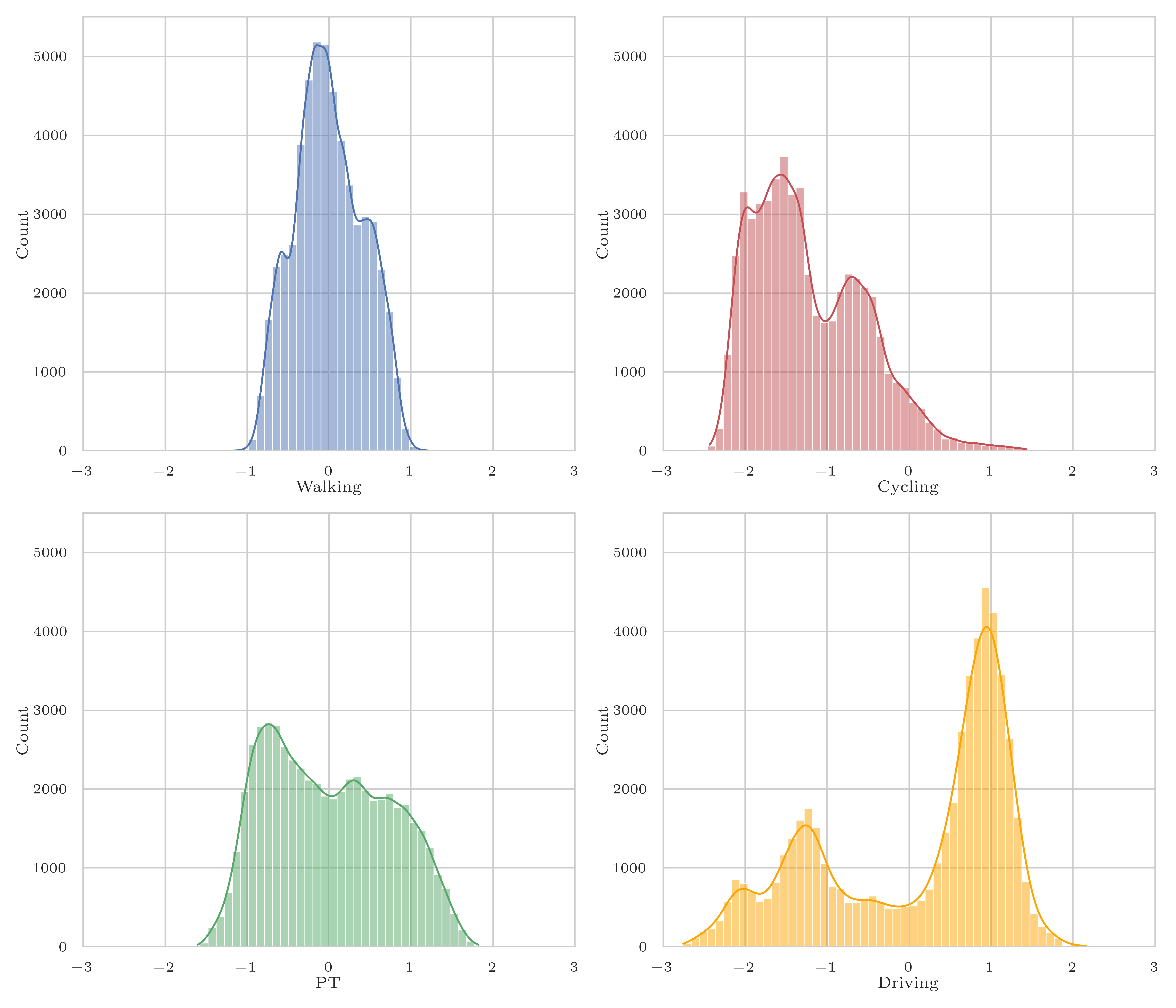
Figure 8: Histograms of the individual-specific constant learnt with the Functional Effect RUMBoost of a) walking, b) cycling, c) PT and d) driving alternative. For each histogram, we plot the kernel density estimate as a solid line. Overall, cycling, PT and driving individual constants exhibit a bi-modal distribution, and walking alternative a uni-modal distribution centered at zero.

These three extensions demonstrate the RUMBoost model’s ability to incorporate attribute interactions, account for correlated error terms within alternatives, and learn an individual-specific constant for observation correlated data. The extensions can also be combined, as they are applied to different parts of the model. This showcases the flexibility and generalisability of the RUMBoost framework. In future work, any complex choice situations that lead to a defined gradient and hessian could be applied to the model.

5 Conclusion and further work

The methodology presented in this paper allows for a fully interpretable ML model (RUMBoost) based on GBDT and inspired by random utility models. In short, RUMBoost replaces every parameter of a RUM by an ensemble of regression trees. By re-implementing classification for GBDT, we can provide specific attributes for alternative utilities, control attribute interactions in the ensemble, and apply monotonic constraints on key attributes based on domain knowledge. These constraints considerably improve the predictions of traditional RUMs and enable the derivation of non-linear utility functions. Furthermore, we apply piece-wise monotonic cubic splines to interpolate the utility functions and obtain a smooth utility function. We find that the smoothing acts as further regularization and enables us to compute the Value of Time (VoT). We also show that the modularity of our approach allow for the estimation of complex model specification such as error term accounting for correlation within alternatives or correlation within observations. Our approach offer to observe the full functional form of the utility function with defined gradient, just like in DCMs. The key difference is that the utility function is directly learnt from the data.

Whilst applied here to choice models, this methodology could be used in place of any linear-in-parameters models, for regression, classification, or any task for which the gradient and hessian of the cost function are well defined. Further work includes applying the model to various problems to demonstrate this statement. Further work also includes applying the RUMBoost model to other complex model specifications such as the Cross-Nested Logit (CNL) model. The PCUF algorithm could be improved by applying B-splines, which would provide a $C^{2}$ monotonic interpolation of the data, where shape constraint could be incorporated. Finally, the GBUV could be computed directly with linear trees, quadratic trees or splines, to obtain directly piece-wise utility functions with defined gradient.

CRediT authorship contribution statement

Nicolas Salvadé: Conceptualization, Methodology, Software, Writing - Original Draft, Visualization. Tim Hillel: Conceptualization, Methodology, Writing - Review and Editing, Supervision.

Declaration of competing interest

None

Appendix A Hyperparameter search

Table 8: Hyperparameter search and optimal value for RUMBoost, Nested RUMBoost, and FE-RUMBoost on the LPMC dataset

			RUMBoost	Nested RUMBoost	FE-RUMBoost
Number of searches			1	25	100
Time [s]			44.5	5378	5366
Hyperparameter	Distribution	Search space
Mean of num_iterations	early stopping	100	1300	1256	1099
bagging_fraction	uniform	[0.5, 1]	-	-	0.700
bagging_freq	choice	(0, 1, 5, 10)	-	-	10
feature_fraction	uniform	[0.5, 10]	-	-	0.867
lambda_l1	log uniform	[0.0001, 10]	-	-	6.592
lambda_l2	log uniform	[0.0001, 10]	-	-	1.028
learning_rate	fixed	0.1	-	-	0.1
max_bin	uniform	[100, 500]	-	-	131
min_data_in_leaf	uniform	[1, 200]	-	-	27
min_gain_to_split	log uniform	[0.0001, 5]	-	-	0.800
min_sum_hessian_in_leaf	log uniform	[1,100]	-	-	1.783
num_leaves	uniform	[2, 100]	-	-	74
mu	uniform	[1, 2]	-	1.167	-

Table 9: Hyperparameter search and optimal value for LightGBM, NN, and DNN on the LPMC dataset.

			LightGBM	NN	DNN
Number of searches			1000	1000	1000
Time [s]			24882	28736	26343
Hyperparameter	Distribution	Search space
Mean of CV num_iterations	early stopping	100	1493	-	-
bagging_fraction	uniform	[0.5, 1]	0.7204	-	0.700
bagging_freq	choice	(0, 1, 5, 10)	1	-	10
feature_fraction	uniform	[0.5, 10]	0.6007	-	0.867
lambda_l1	log uniform	[0.0001, 10]	0.0242	-	6.592
lambda_l2	log uniform	[0.0001, 10]	0.0001	-	1.028
learning_rate	fixed	-	0.1	adaptive	0.1
max_bin	discrete uniform	[100, 500]	237	-	131
min_data_in_leaf	discrete uniform	[1, 200]	156	-	27
min_gain_to_split	log uniform	[0.0001, 5]	0.0007	-	0.800
min_sum_hessian_in_leaf	log uniform	[1,100]	1.4136	-	1.783
num_leaves	discrete uniform	[2, 100]	16	-	74
activation	fixed	-	-	$tanh(x)$	$relu(x)$
batch_size	choice	(128, 256, 512, 1024)	-	1024	1024
hidden_layer_size	discrete uniform	[10, 500]	-	-	20
learning_rate_init	uniform	[0.0001, 1]	-	0.0907	-
solver	choice	[lbfgs, sgd, adam]	-	sgd	-
depth	discrete uniform	[2,10]	-	-	2
drop	choice	(0.5, 0.3, 0.1)	-	-	0.3
epochs	discrete uniform	[50, 200]	-	-	90
width	choice	(25, 50, 100, 150, 200)	-	-	50

Appendix B Estimation of the MNL models

Table 10: Parameter estimates of the LPMC MNL. Out of the 62 parameters, 9 are not significant at a 95% confidence interval.

LPMC - MNL
	Value	Active bound	Rob. p-value
ASC_Bike	-3.380	0.000	0.000
ASC_Car	-2.592	0.000	0.000
ASC_Public_Transport	-1.908	0.000	0.000
B_age_Bike	-0.004	0.000	0.032
B_age_Car	0.005	0.000	0.000
B_age_Public_Transport	0.011	0.000	0.000
B_car_ownership_Bike	0.036	0.000	0.590
B_car_ownership_Car	0.694	0.000	0.000
B_car_ownership_Public_Transport	-0.213	0.000	0.000
B_con_charge_Car	-1.147	0.000	0.000
B_cost_driving_fuel_Car	0.000	1.000	1.000
B_cost_transit_Public_Transport	-0.115	0.000	0.000
B_day_of_week_Bike	-0.020	0.000	0.201
B_day_of_week_Car	0.030	0.000	0.000
B_day_of_week_Public_Transport	-0.044	0.000	0.000
B_distance_Bike	-0.232	0.000	0.040
B_distance_Car	0.000	1.000	1.000
B_distance_Public_Transport	0.000	1.000	1.000
B_driving_license_Bike	0.678	0.000	0.000
B_driving_license_Car	0.663	0.000	0.000
B_driving_license_Public_Transport	-0.526	0.000	0.000
B_dur_cycling_Bike	-2.670	0.000	0.000
B_dur_driving_Car	-4.777	0.000	0.000
B_dur_pt_access_Public_Transport	-4.608	0.000	0.000
B_dur_pt_bus_Public_Transport	-1.911	0.000	0.000
B_dur_pt_int_waiting_Public_Transport	-4.284	0.000	0.000
B_dur_pt_int_walking_Public_Transport	-2.335	0.000	0.027
B_dur_pt_rail_Public_Transport	-1.338	0.000	0.000
B_dur_walking_Walk	-8.596	0.000	0.000
B_female_Bike	-0.834	0.000	0.000
B_female_Car	0.100	0.000	0.002
B_female_Public_Transport	0.160	0.000	0.000
B_fueltype_Avrg_Bike	-0.691	0.000	0.000
B_fueltype_Avrg_Car	-1.400	0.000	0.000
B_fueltype_Avrg_Public_Transport	-0.221	0.000	0.000
B_fueltype_Diesel_Bike	-0.822	0.000	0.000
B_fueltype_Diesel_Car	-0.228	0.000	0.000
B_fueltype_Diesel_Public_Transport	-0.419	0.000	0.000
B_fueltype_Hybrid_Bike	-1.000	0.000	0.000
B_fueltype_Hybrid_Car	-0.721	0.000	0.000
B_fueltype_Hybrid_Public_Transport	-0.945	0.000	0.000
B_fueltype_Petrol_Bike	-0.867	0.000	0.000
B_fueltype_Petrol_Car	-0.242	0.000	0.000
B_fueltype_Petrol_Public_Transport	-0.323	0.000	0.000
B_pt_n_interchanges_Public_Transport	-0.101	0.000	0.154
B_purpose_B_Bike	-0.029	0.000	0.775
B_purpose_B_Car	-0.043	0.000	0.543
B_purpose_B_Public_Transport	-0.012	0.000	0.874
B_purpose_HBE_Bike	-1.054	0.000	0.000
B_purpose_HBE_Car	-0.756	0.000	0.000
B_purpose_HBE_Public_Transport	-0.237	0.000	0.000
B_purpose_HBO_Bike	-0.773	0.000	0.000
B_purpose_HBO_Car	-0.352	0.000	0.000
B_purpose_HBO_Public_Transport	-0.442	0.000	0.000
B_purpose_HBW_Bike	-0.291	0.000	0.000
B_purpose_HBW_Car	-1.062	0.000	0.000
B_purpose_HBW_Public_Transport	-0.502	0.000	0.000
B_purpose_NHBO_Bike	-1.233	0.000	0.000
B_purpose_NHBO_Car	-0.379	0.000	0.000
B_purpose_NHBO_Public_Transport	-0.715	0.000	0.000
B_start_time_linear_Bike	0.017	0.000	0.015
B_start_time_linear_Car	0.027	0.000	0.000
B_start_time_linear_Public_Transport	0.010	0.000	0.016
B_traffic_perc_Car	-2.404	0.000	0.000

Table 11: Parameter estimates of the LPMC NL. Out of the 63 parameters, 10 are not significant at a 95% confidence interval.

LPMC - NL
	Value	Active bound	Rob. p-value
ASC_Bike	-3.346	0.000	0.000
ASC_Car	-2.439	0.000	0.000
ASC_Public_Transport	-1.969	0.000	0.000
B_age_Bike	-0.004	0.000	0.026
B_age_Car	0.007	0.000	0.000
B_age_Public_Transport	0.011	0.000	0.000
B_car_ownership_Bike	0.062	0.000	0.351
B_car_ownership_Car	0.628	0.000	0.000
B_car_ownership_Public_Transport	-0.037	0.000	0.369
B_con_charge_Car	-0.816	0.000	0.000
B_cost_driving_fuel_Car	0.000	1.000	1.000
B_cost_transit_Public_Transport	-0.077	0.000	0.000
B_day_of_week_Bike	-0.023	0.000	0.155
B_day_of_week_Car	0.022	0.000	0.007
B_day_of_week_Public_Transport	-0.033	0.000	0.000
B_distance_Bike	-0.225	0.000	0.042
B_distance_Car	-0.005	0.000	0.960
B_distance_Public_Transport	0.000	1.000	1.000
B_driving_license_Bike	0.705	0.000	0.000
B_driving_license_Car	0.484	0.000	0.000
B_driving_license_Public_Transport	-0.396	0.000	0.000
B_dur_cycling_Bike	-1.839	0.000	0.003
B_dur_driving_Car	-3.409	0.000	0.000
B_dur_pt_access_Public_Transport	-3.410	0.000	0.000
B_dur_pt_bus_Public_Transport	-1.445	0.000	0.000
B_dur_pt_int_waiting_Public_Transport	-3.036	0.000	0.000
B_dur_pt_int_walking_Public_Transport	-1.876	0.000	0.017
B_dur_pt_rail_Public_Transport	-1.085	0.000	0.000
B_dur_walking_Walk	-8.171	0.000	0.000
B_female_Bike	-0.831	0.000	0.000
B_female_Car	0.112	0.000	0.000
B_female_Public_Transport	0.156	0.000	0.000
B_fueltype_Avrg_Bike	-0.680	0.000	0.000
B_fueltype_Avrg_Car	-1.175	0.000	0.000
B_fueltype_Avrg_Public_Transport	-0.322	0.000	0.000
B_fueltype_Diesel_Bike	-0.817	0.000	0.000
B_fueltype_Diesel_Car	-0.251	0.000	0.000
B_fueltype_Diesel_Public_Transport	-0.391	0.000	0.000
B_fueltype_Hybrid_Bike	-0.985	0.000	0.000
B_fueltype_Hybrid_Car	-0.755	0.000	0.000
B_fueltype_Hybrid_Public_Transport	-0.941	0.000	0.000
B_fueltype_Petrol_Bike	-0.864	0.000	0.000
B_fueltype_Petrol_Car	-0.259	0.000	0.000
B_fueltype_Petrol_Public_Transport	-0.315	0.000	0.000
B_pt_n_interchanges_Public_Transport	-0.088	0.000	0.093
B_purpose_B_Bike	-0.032	0.000	0.748
B_purpose_B_Car	-0.066	0.000	0.337
B_purpose_B_Public_Transport	-0.053	0.000	0.445
B_purpose_HBE_Bike	-1.036	0.000	0.000
B_purpose_HBE_Car	-0.665	0.000	0.000
B_purpose_HBE_Public_Transport	-0.271	0.000	0.000
B_purpose_HBO_Bike	-0.771	0.000	0.000
B_purpose_HBO_Car	-0.317	0.000	0.000
B_purpose_HBO_Public_Transport	-0.397	0.000	0.000
B_purpose_HBW_Bike	-0.272	0.000	0.000
B_purpose_HBW_Car	-0.976	0.000	0.000
B_purpose_HBW_Public_Transport	-0.570	0.000	0.000
B_purpose_NHBO_Bike	-1.235	0.000	0.000
B_purpose_NHBO_Car	-0.415	0.000	0.000
B_purpose_NHBO_Public_Transport	-0.678	0.000	0.000
B_start_time_linear_Bike	0.016	0.000	0.016
B_start_time_linear_Car	0.024	0.000	0.000
B_start_time_linear_Public_Transport	0.012	0.000	0.002
B_traffic_perc_Car	-1.947	0.000	0.000
MU_m	1.391	0.000	0.000

References

- Aboutaleb (2022) Aboutaleb, Y.M., 2022. Theory-constrained Data-driven Model Selection, Specification, and Estimation: Applications in Discrete Choice Models. Ph.D. thesis. Massachusetts Institute of Technology.
- Ben-Akiva and Lerman (1985) Ben-Akiva, M.E., Lerman, S.R., 1985. Discrete choice analysis: theory and application to travel demand. MIT Press series in transportation studies, MIT Press, Cambridge, Mass.
- Bergstra et al. (2013) Bergstra, J., Yamins, D., Cox, D., 2013. Making a science of model search: Hyperparameter optimization in hundreds of dimensions for vision architectures, in: International conference on machine learning, PMLR. pp. 115–123.
- Bierlaire (2023) Bierlaire, M., 2023. A short introduction to Biogeme. Technical Report. Technical report TRANSP-OR 230620. Transport and Mobility Laboratory, ENAC, EPFL.
- Caruana et al. (2015) Caruana, R., Lou, Y., Gehrke, J., Koch, P., Sturm, M., Elhadad, N., 2015. Intelligible models for healthcare: Predicting pneumonia risk and hospital 30-day readmission, in: Proceedings of the 21th ACM SIGKDD international conference on knowledge discovery and data mining, pp. 1721–1730.
- Chen and Guestrin (2016) Chen, T., Guestrin, C., 2016. XGBoost: A Scalable Tree Boosting System, in: Proceedings of the 22nd ACM SIGKDD International Conference on Knowledge Discovery and Data Mining, pp. 785–794. URL: http://arxiv.org/abs/1603.02754, doi:10.1145/2939672.2939785. arXiv:1603.02754 [cs].
- Dahmen et al. (2023) Dahmen, V., Weikl, S., Bogenberger, K., 2023. Interpretable machine learning for mode choice modeling on 1 tracking-based revealed preference data 2. Victoria 4, 5.
- Friedman (2001) Friedman, J.H., 2001. Greedy function approximation: A gradient boosting machine. The Annals of Statistics 29. doi:10.1214/aos/1013203451.
- Fritsch and Butland (1984) Fritsch, F.N., Butland, J., 1984. A method for constructing local monotone piecewise cubic interpolants. SIAM journal on scientific and statistical computing 5, 300–304.
- Fritsch and Carlson (1980) Fritsch, F.N., Carlson, R.E., 1980. Monotone piecewise cubic interpolation. SIAM Journal on Numerical Analysis 17, 238–246.
- Han et al. (2022) Han, Y., Pereira, F.C., Ben-Akiva, M., Zegras, C., 2022. A neural-embedded discrete choice model: Learning taste representation with strengthened interpretability. Transportation Research Part B: Methodological 163, 166–186.
- Hastie and Tibshirani (1990) Hastie, T.J., Tibshirani, R.J., 1990. Generalized additive models. volume 43. CRC press.
- Hillel (2019) Hillel, T., 2019. Understanding travel mode choice: A new approach for city scale simulation. Ph.D. thesis. University of Cambridge.
- Hillel et al. (2019) Hillel, T., Bierlaire, M., Elshafie, M., Jin, Y., 2019. Weak teachers: Assisted specification of discrete choice models using ensemble learning, in: 8th Symposium of the European association for research in transportation, Budapest.
- Hillel et al. (2018) Hillel, T., Elshafie, M.Z.E.B., Jin, Y., 2018. Recreating passenger mode choice-sets for transport simulation: A case study of London, UK. Proceedings of the Institution of Civil Engineers - Smart Infrastructure and Construction 171, 29–42. URL: https://www.icevirtuallibrary.com/doi/10.1680/jsmic.17.00018, doi:10.1680/jsmic.17.00018.
- Ke et al. (2017) Ke, G., Meng, Q., Finley, T., Wang, T., Chen, W., Ma, W., Ye, Q., Liu, T.Y., 2017. Lightgbm: A highly efficient gradient boosting decision tree. Advances in neural information processing systems 30.
- Kim and Bansal (2023) Kim, E.J., Bansal, P., 2023. A new flexible and partially monotonic discrete choice model. Available at SSRN 4448172 .