The Ensemble Kalman filter for dynamic
inverse problems

Abstract.

In inverse problems, the goal is to estimate unknown model parameters from noisy observational data. Traditionally, inverse problems are solved under the assumption of a fixed forward operator describing the observation model. In this article, we consider the extension of this approach to situations where we have a dynamic forward model, motivated by applications in scientific computation and engineering. We specifically consider this extension for a derivative-free optimizer, the ensemble Kalman inversion (EKI). We introduce and justify a new methodology called dynamic-EKI, which is a particle-based method with a changing forward operator. We analyze our new method, presenting results related to the control of our particle system through its covariance structure. This analysis includes moment bounds and an ensemble collapse, which are essential for demonstrating a convergence result. We establish convergence in expectation and validate our theoretical findings through experiments with dynamic-EKI applied to a 2D Darcy flow partial differential equation.

1. Introduction

The focus of this work is on the research area of inverse problems [2, 33, 36], which is involves learning parameters, of quantities of interest from observations which are corrupted by noise. In many instances of inverse problems, one usually adopts a setting where the dynamics generating the observations, i.e., the model of interest, is fixed and independent of time. However, there are highly relevant applications where the dynamics related to the forward operator change within each time frame, resulting in new observations. Such applications include geophysical sciences, numerical weather prediction such as the Naiver-Stokes equation and electrical resistivity tomography from thermodynamics [28, 31]. This motivates the use of a time-dependent forward operator within inverse problems, where the observation of the unknown of interest changes over time. Modifying traditional inverse problems in the setup we described poses computational and mathematical challenges, which has resulted in very limited literature. Our aim is to overcome and tackle these challenges, in the context of inverse problems and, in particular, where we exploit a particular inverse problem methodology known as the ensemble Kalman inversion [8, 21, 27].

1.1. Preliminaries

Before we introduce the notion of ensemble Kalman inversion (EKI), we present the mathematical formulation of an inverse problem. Throughout this manuscript we consider an underlying probability space $(\Omega,\mathcal{F},\mathbb{P})$. Given a set of noisy observations $u\in\mathbb{R}^{p}$, we are interested in recovering some unknown parameter $z\in\mathbb{R}^{d}$, where the relationship between both is defined as

(1.1) $$u=S(z)+w,\quad w\sim\mathcal{N}(0,\Gamma)\,.$$

Here, $S:\mathbb{R}^{d}\to\mathbb{R}^{p}$ is the forward operator and we assume our data is corrupted by additive Gaussian noise. We will use this assumption throughout this work. Commonly, inverse problems are ill-posed and require some regularization scheme to produce numerical solutions. One method, which is the method of interest in this article, is the application of EKI as derivative-free optimizer for solving the minimization procedure

(1.2) $$\min_{z\in\mathbb{R}^{d}}J(z),\quad J(z)=\frac{1}{2}\|S(z)-u\|^{2}_{\Gamma}+\frac{\alpha}{2}\|z\|^{2},$$

where the final term of our objective functional $J$ is a penalty term acting as regularization with regularization parameter $\alpha>0$. This specific penalty term in (1.2) corresponds to Tikhonov regularization. Traditionally, to solve (1.2) one must resort to gradient methods. EKI instead operates by updating an ensemble of particles $z^{(j)}_{n}$, where $1\leq j\leq J$ denotes the ensemble member index, using sample covariances which replace the computation of gradients. We define the following sample means and sample covariances

$$\bar{z}_{n}=\frac{1}{J}\sum_{j=1}^{J}z_{n}^{(j)},\quad\bar{S}_{n}=\frac{1}{J}\sum_{j=1}^{J}S(z_{n}^{(j)}),$$

$$C_{n}^{zz}=\frac{1}{J}\sum_{j=1}^{J}(z_{n}^{(j)}- \bar{z}_{n})(z_{n}^{(j)}-\bar{z}_{n})^{\top},\quad C_{n}^{zp}=\frac{1}{J}\sum_{j=1}^{J}(z_{n}^{(j)}-\bar{z}_{n})(S(z_{n}^{(j)})-\bar{S}_{n})^{\top}\,.$$

The update formulae for EKI are then given as

(1.3) $$z_{n+1}^{(j)}=z_{n}^{(j)}+C_{n}^{zz}(C_{n}^{zp}+\Gamma)^{-1}(u_{n+1}^{(j)}-S(z_{n}^{(j)})),$$

(1.4) $$u_{n+1}^{(j)}=u+w^{(j)}_{n+1},$$

where $(u_{n}^{(j)})$ are perturbed observations with independent realizations of the observational noise $w^{(j)}_{n}\sim\mathcal{N}(0,\Gamma)$. The above formulation of EKI was originally derived in [21], and motivated through the ensemble Kalman filter, and its application in reservoir modelling [15, 16, 27, 37]. Since this seminal work, numerous extensions, and developments, have been made which include deriving regularization schemes, in particular Tikhonov regularization [10, 20, 22, 41], deriving analysis both in the continuous and discrete setting [3, 4, 5, 9, 11, 32, 38, 43] and providing connections with sampling and mean-field analysis [14, 18]. With all these developed works, EKI has thus far only been considered in a framework where the operator $S:\mathbb{R}^{d}\rightarrow\mathbb{R}^{p}$ is static. As mentioned, in the context of inverse problems, it is an important extension to time-dependent forward models where limited literature exists. Our specific interest is the potential connection with the EKI methodology. Time-dependent inverse problems are a relatively new field of interest, which are motivated through the use of some natural applications. Some of the recent research in this field are through the development of new methodology, such as Kaczmarz-based methods, for linear time-dependent problems, as well as developing theory through the use of Bochner spaces, and the connections to well-known models in applied mathematics such as the Fokker-Planck equation [1, 24, 25, 26, 30].

1.2. Problem formulation

We consider the task of recovering an underlying groundtruth $z_{\ast}\in\mathbb{R}^{d}$, given a time-dependent observation model (in discrete time) of form

(1.5) $$u_{t}=S_{t}z_{\ast}+w_{t},\quad t\in\mathbb{N}\,,$$

where $S_{t}\in\mathbb{R}^{p\times d}$ denotes the dynamic, possibly stochastic, observation operator mapping to a lower dimensional observation space $\mathbb{R}^{p}$. We will assume that the sequence of observation operators $(S_{t})_{t\in\mathbb{N}}$ is either aperiodic and ergodic, or periodic. For each fixed time $t\in\mathbb{N}$ we assume that the observation operator $S_{t}$ is linear. Moreover, we assume that the observation is perturbed by independent and identically distributed (iid) noise $(w_{t})_{t\in\mathbb{N}}$ with $w_{t}\sim\mathcal{N}(0,\Gamma)$, $t\in\mathbb{N}$, where $\Gamma\in\mathbb{R}^{p\times p}$ is assumed to be symmetric and positive definite. In the following, we denote the natural filtration generated by $(u_{t})_{t\in\mathbb{N}}$ as $\mathcal{F}_{t}=\sigma(u_{s},s\leq t)$. Note that $(w_{s})_{s>t}$ is independent of $\mathcal{F}_{t}$ by construction. Given a sequence of observations $(u_{t})_{t\in\mathbb{N}}$ we want to recover the groundtruth $z_{\ast}$ sequentially.

In order to discuss the relevance of the considered observation model (1.5), we consider a number of useful examples. Further example are provided in the following book which is a collection of works on time-dependent inverse problems [25], such as molecular localization microscopy, acoustic parameter imaging and others. We now present two model examples, where the first one of them is studied numerically in more details in Section 5.

Example 1.1 (Darcy flow).

We consider the following $2$-dimensional elliptic PDE model

(1.6) $$\begin{cases}-\nabla\cdot(\exp(a)\nabla p)=z^{\ast},&x\in D\\ p=0,&x\in\partial D\end{cases}\,,$$

with domain $D:=(0,1)^{2}$ and subject to zero Dirichlet boundary conditions. Our aim is to recover the unknown source term $z^{\ast}\in L^{\infty}(D)$ from discrete observation points of the solution $p\in\mathcal{V}:=H_{0}^{1}(D)\cap H^{2}(D)$. Given $a\in L^{\infty}(D)$ let $G_{a}:L^{\infty}(D)\to\mathcal{V}$ denote the solution operator of (1.6) and define an observation operator to be a linear operator $\mathcal{O}_{[x_{1}:x_{k}]}:\mathcal{V}\to\mathbb{R}^{K}$ that evaluates $p\in\mathcal{V}$ in $K$ specified observation points $x_{1},\dots,x_{K}\in D$. More precisely, this means $\mathcal{O}_{[x_{1}:x_{k}]}p=(p(x_{1}),\dots,p(x_{K}))^{\top}\in\mathbb{R}^{K}$. We are interested in recovering $z^{\ast}$ given a sequence of observations

$$u_{t}=\mathcal{O}_{t}\circ G_{t}(z^{\ast})+w_{t}\,,$$

where either the solution operator or the observation operator, or both, change in time. Moreover, in each observation step we assume that $w_{t}\sim\mathcal{N}(0,\Gamma)$ is independent additive Gaussian noise. In the following, we present a row of specific observation models in which we are interested.

• Independent observation model: One simple scenario would be the case where $a$ is fixed, but for each measurement the observation operator draws observation points uniformly and independently in $D$. This means, we define $\mathcal{O}_{t}:=\mathcal{O}_{[x_{1}(t):x_{K}(t)]}$ where $x_{i}(t)\sim\mathcal{U}(D)$ are independent for all $i=1,\dots,K$ and $t\geq 1$. In this case, we consider a sequence of observations given by

  $$u_{t}=S_{t}z^{\ast}+w_{t},$$

  where $S_{t}:=\mathcal{O}_{t}\circ G$ with $G:=G_{a}$.

• Periodic observation model: Next, we consider the case where the domain $D$ can be decomposed into $p$ disjoint subsets $D_{1},\dots,D_{p}\subset D$ such that $D=\cup_{i=1}^{p}D_{i}$. We then define the dynamic observation operator by first selecting a subdomain $j$ and then drawing independently observation points in $D_{j}$. More precisely, for $t=pk+i$ for $k\geq 0$ and $i=1,\dots p$ we define $\mathcal{O}_{t}=\mathcal{O}_{[x_{1}(t):x_{K}(t)]}$ where $x_{i}(t)\sim\mathcal{U}(D_{i}),i\in[K],$ independently. Hence, we move periodically through all sub-domains $D_{1},\dots D_{p}$ and take observations. The sequence of observations is again given by

  $$u_{t}=S_{t}z^{\ast}+w_{t},$$

  with $S_{t}:=\mathcal{O}_{t}\circ G$ and $G:=G_{a}$ for a fixed $a$.

• Ergodic observation model: In the last setting, we assume that the observation operator is fixed and given by $\mathcal{O}:=\mathcal{O}_{[x_{1}:x_{K}]}$ for $x_{1},\dots,x_{K}\in\mathcal{D}$. However, we assume that the diffusion coefficient $a$ is dynamic. Suppose that $(a_{t})_{t\geq 0}$ is generated from an ergodic Markov chain and define for each state $a_{t}$ the solution operator $G_{t}=G_{a_{t}}$. This Markov chain may come for example from a Markov chain Monte Carlo algorithm targeting some posterior distribution from a pre-stage Bayesian experiment. In this case, we consider a sequence of observations

  $$u_{t}=S_{t}z^{\ast}+w_{t},$$

  where this time the dynamic forward model is defined by $S_{t}:=\mathcal{O}\circ G_{t}$.

We emphasize that this list of examples is by far not complete and the different types of observation models may further be combined. For example, in (ii) one may also consider the case where the sub-domain is picked by some agent who follows a specific decision rule. This may lead again to a limiting ergodic behavior.

In order to reconstruct the underlying ground truth $z_{\ast}$, the goal is to solve an optimization problem of form

(1.7) $$\min_{z\in\mathbb{R}^{d}}\ J(z),\quad J(z):=\ell(z-z_{\ast})+\frac{\alpha}{2}\|z\|^{2},\quad\ell(v):=v^{\top}Av=\|Sv\|^{2}\,,$$

where $\alpha>0$ denotes a suitable regularization parameter. Note that we assume that $\alpha>0$ has been chosen and is given as fixed parameter. However, we emphasize that the performance of the reconstruction of $z_{\ast}$ will heavily depend on the choice of $\alpha$. Deriving specific choices of the regularization parameter $\alpha>0$ is left for future work.

The key challenge in the time-dependent setting for solving the optimization problem (1.7), is that the limiting matrix $A$ and the underlying groundtruth $z_{\ast}$ are unknown, and $z_{\ast}$ can only be observed through the (random) observation operator $S_{t}$ perturbed by noise $w_{t}$, i.e. through the sequence of observations $(u_{t})_{t\in\mathbb{N}}$ defined in (1.5). Note that the solution of the minimization problem can be written analytically depending on the unknown matrix $A$ and $z_{\ast}$ as

$$z^{\mathrm{opt}}=(S^{\top}S+\alpha I)^{-1}S^{\top}u_{\infty},\quad u_{\infty}:=Sz_{\ast}\,,$$

which solves the first order optimality condition

$$0=\nabla J(z)=S^{\top}(Sz-u_{\infty})+\alpha z\,.$$

We collect the following notations

$$A=S^{\top}S,\quad A^{(\alpha)}=S^{\top}S+\alpha I,\quad A_{t}=S_{t}^{\top}S_{t},\quad A_{t}^{(\alpha)}=S_{t}^{\top}S_{t}+\alpha I\,,$$

and observe that we can write $J(z)=\langle z,A^{(\alpha)}z\rangle$, where $\langle\cdot,\cdot\rangle$ denotes the euclidean inner product. Moreover, we have the connection $A^{(\alpha)}z^{\mathrm{opt}}=Az_{\ast}$, $A_{t}-A=A_{t}^{(\alpha)}-A^{(\alpha)}$ and

$$\nabla J(z)=A^{(\alpha)}z-Az_{\ast}\,.$$

In the upcoming section, we will discuss assumptions on the relation between $S_{t}$ and $A$ in more details.

1.3. Model assumptions

As mentioned, within this work we will consider two forms of data models which are (i) ergodic data, and (ii) periodic data. Note that iid data can be viewed as special case of both models. To help distinguish each form of data we discuss numerous assumptions related to each data form.

Ergodic data

We begin by making the following asymptotic assumption on the dynamic forward operator when using ergodic data.

Assumption 1.2 (ergodic data).

Let $(S_{t})_{t\in\mathbb{N}}$ with $S_{t}\in\mathbb{R}^{p\times d}$ be a sequence of $\mathcal{F}_{t}$-adapted (random) matrices such that there exists a symmetric positive definite and bounded matrix $A\in\mathbb{R}^{d\times d}$, i.e. $0\preceq A\preceq I$, satisfying the following limiting behaviour. For any $\varepsilon>0$ there is an $\tau_{\varepsilon}\gtrsim|\log(\varepsilon^{-1})|>0$ such that

$$\|\mathbb{E}[S_{t+1+\tau_{\varepsilon}}^{\top}S_{t+1+\tau_{\varepsilon}}\mid\mathcal{F}_{t}]-A\|=\|\mathbb{E}[A_{t+1+\tau_{\varepsilon}}\mid\mathcal{F}_{t}]-A\|\leq\varepsilon\,,$$

for all $t\geq 1$.

Assumption 1.2 is motivated by the ergodic theory of Markov process [29]. In particular, $\tau_{\epsilon}$ is often interpreted as the mixing time of the process, which describes how fast the process does converge to the stationary distribution. Since the convergence speed is in general exponential, $\tau_{\epsilon}$ often scales as $\mathcal{O}(\log\epsilon)$. The matrix $A$ in Assumption 1.2 is the average of $A_{t}$ under the stationary distribution.

Remark 1.3.

We emphasize that Assumption 1.2 is substantially weaker than assuming that the data is generated from an iid sequence of observations. As result our presented convergence result directly transfer and even simplifies under assumption of iid data, where we assume that $(S_{t})_{t\in\mathbb{N}}$ is a sequence of independent and identically distributed (random) matrices such that

$$\mathbb{E}[S_{t}^{\top}S_{t}]=S^{\top}S=A,$$

where the expectation matrix $A\in\mathbb{R}^{d\times d}$ is assumed to be positive definite and bounded, i.e. $0\preceq A\preceq I$.

Periodic data

Our second form of data we consider in this work is periodic data. Since Assumption 1.2 is known to fail for periodic Markov Chains, we describe our next assumption of periodic limiting behavior of the considered time-dynamical observation model. Note that this assumption also allows for randomness in the time-dependent model.

Assumption 1.4 (periodic data).

Let $(S_{t})_{t\in\mathbb{N}}$ with $S_{t}\in\mathbb{R}^{p\times d}$ be a sequence of (random) matrices such that there exists a positive definite and bounded matrix $A\in\mathbb{R}^{d\times d}$, i.e. $0\preceq A\preceq I$, satisfying the following limiting behaviour. For any $\varepsilon>0$ there is an $\tau_{\varepsilon}\gtrsim|\varepsilon^{-1}|>0$ such that

$$\Big{\|}\mathbb{E}[\frac{1}{\tau_{\varepsilon}}\sum_{k=0}^{\tau_{\varepsilon}-1}S_{t+1+k}^{\top}S_{t+1+k}\mid\mathcal{F}_{t}]-A\Big{\|} =\Big{\|}\frac{1}{\tau_{\varepsilon}}\sum_{k=0}^{\tau_{\varepsilon}-1}\mathbb{E}[A_{t+1+k}\mid\mathcal{F}_{t}]-A\Big{\|}$$

$$=:\Big{\|}\frac{1}{\tau_{\varepsilon}}\mathbb{E}[A_{(t+1):(t+1+\tau_{\varepsilon})}\mid\mathcal{F}_{t}]-A\Big{\|}\leq\varepsilon\,,$$

for all $t\geq 1$.

Considering periodic data is interesting for a number of reasons, firstly because the extension covers the case where $S_{t}$ is a periodic sequence, whereas the cases of Assumption 1.2 does not cover periodic sequences.

1.4. Our Contributions:

To conclude this section, we summarize our contributions below.

• We present a formulation of the ensemble Kalman inversion based on the time-dependent observation model (1.5). This differs from the conventional EKI, where the forward operator $S$ is usually assumed to be fixed and is applied as tool in a static inverse problems setting. Our resulting algorithm is entitled “dynamic EKI”.

• We provide a number of theoretical results to demonstrate the validity of our proposed scheme. Our initial analysis require the controlling of the modified covariance matrix, for which we demonstrate this through lower and upper bounds on the ensemble collapse, and providing moment bounds.

• A convergence analysis is provided for the dynamic-EKI as stochastic optimization method of (1.7). This analysis covers the three different data types of interest: (i) iid data, (ii) ergodic data and (iii) periodic data.

• Numerical experiments are conducted verifying the theory that is attained. We test our dynamic-EKI on a 2D Darcy flow PDE example, comparing our ergodic, periodic and iid data.

1.5. Outline

The outline of this work is as follows: In Section 2 we describe and provide our dynamic version of EKI. This will lead onto Section 3 which is where our preliminary analysis is presented. Section 4 is devoted to the proof of our theorems, which are seperated based on the type of data that is used. Numerical results are shown in Section 5 and finally, we conclude our findings in Section 6.

2. Ensemble Kalman inversion with dynamic forward operator

In this section we introduce and discuss our proposed algorithm, referred to as dynamic-EKI. In order to derive it, we firstly present the vanilla version of EKI (1.3) in a modified setting, which provides strong differences. We finish this section by stating our main result which is a convergence theorem for dynamic-EKI with given rate of convergence.

One possible way to solve (1.7), is to apply a gradient descent scheme. Since we assume that there is no access to $A$, $S$ and $z_{\ast}$, we may formulate the dynamic (stochastic) gradient descent scheme by

(2.1) $$z_{t+1}=z_{t}-\eta_{t}\nabla J_{t+1}(z_{t})=z_{t}-\eta_{t}\left(S_{t+1}^{\top}(S_{t+1}z_{t}-u_{t+1})+\alpha z_{t}\right)\,,$$

with initial $z_{0}\in\mathbb{R}^{d}$, $t\in\mathbb{N}$, where $(\eta_{t})_{t\in\mathbb{N}}$ with $\eta_{t}>0$, $t\in\mathbb{N}$ denotes a sequence of step sizes, and $J_{t}:\mathbb{R}^{d}\to\mathbb{R}$ denotes the time-dependent loss function defined by

(2.2) $$J_{t}(v)=\|S_{t}v-u_{t}\|^{2}+\frac{\alpha}{2}\|v\|^{2},\quad t\in\mathbb{N}\,.$$

We propose to apply an alternative algorithm motivated by the EKI, which can be written in simplified form as

(2.3) $$z_{t+1}^{(j)}=z_{t}^{(j)}-\eta_{t}C_{t}^{zz}\left(S_{t+1}^{\top}(S_{t+1}z_{t}^{(j)}-u_{t+1})+\alpha z_{t}^{(j)}\right),$$

where our sample covariance and mean are defined as

$$C_{t}^{zz}=\frac{1}{J}\sum_{j=1}^{J}(z_{t}^{(j)}-\bar{z}_{t})(z_{t}^{(j)}-\bar{z}_{t})^{\top},\quad\bar{z}_{t}=\frac{1}{J}\sum_{j=1}^{J}z_{t}^{(j)}.$$

Note that an alternative formulation of the ensemble Kalman inversion incorporates perturbed observations such that the iteration can be written as

(2.4) $$\begin{split}z_{t+1}^{(j)}&=z_{t}^{(j)}-\eta_{t}C_{t}^{zz}\left(S_{t+1}^{\top}(S_{t+1}z_{t}^{(j)}-u_{t+1}^{(j)})+\alpha z_{t}^{(j)}\right),\\ u_{t+1}^{(j)}&=S_{t+1}z_{\ast}+w_{t+1}^{(j)},\end{split}$$

where $w_{t}^{(j)}\sim\mathcal{N}(0,\Gamma)$ are assumed to be independent realizations of the noise. Based on this, we present our new methodology in Algorithm 1. Note that the interacting particle system generated by (2.3) or (2.4) respectively are adapted with respect to the filtration $(\mathcal{F}_{t})_{t\in\mathbb{N}}$ by construction. In our convergence results we focus on the dynamic-EKI with unperturbed observations (2.3).

1:Input:

• initial ensemble $z_{0}^{(i)}\in\mathbb{R}^{d}$, $i=1,\dots,J$,

• sequence step sizes $(\eta_{t})_{t\in\mathbb{N}}$.

2:for $t=1,\dots,T$ do

3:     perturb observations $u_{t+1}^{(j)}\sim\mathcal{N}(u_{t+1},\eta_{t}^{-1}\Gamma)$,

4:     for $j=1,\dots,J$ iterate

$$z_{t+1}^{(j)}=z_{t}^{(j)}-\eta_{t}C_{t}^{zz}\left(S_{t+1}^{\top}(S_{t+1}z_{t}^{(j)}-u_{t+1}^{(j)})+\alpha z_{t}^{(j)}\right)\,,$$

5:     set $\bar{z}_{t}=\frac{1}{J}\sum_{i=1}^{J}z_{t}^{(i)}$.

6:end for

Algorithm 1 Dynamic Ensemble Kalman Inversion (DEKI)

The above formulation for our dynamic-EKI may seem quite different to its original form, presented in (1.3)-(1.4). To help to understand the intuition behind it we briefly discuss and present the connection to gradient related algorithms which follow similar ideas. Assuming that $S_{t}^{\top}S_{t}$ is an independent and unbiased estimator of $S^{\top}S=A$ for each $t\in\mathbb{N}$, we can view (2.1) as specific form of stochastic gradient descent (SGD), where for each $t\in\mathbb{N}$ one can verify

$$\mathbb{E}[\nabla J_{t+1}(z_{t})\mid\mathcal{F}_{t}]=\nabla J(z_{t})\,.$$

As result, our proposed dynamic-EKI can be viewed as preconditioned SGD algorithm. Indeed, under this assumption, we may view (2.3) as discrete time variant of of the subsampling approach for EKI recently proposed by Hanu et al. [19]. In that work the authors provided a subsampling approach to EKI in the continuous-time formulation, where the different observations are chosen using switching times. It is worthy to point out that no particular rate of convergence was derived, as a continuous-time setting was primarily adopted. As result we can view the iid setting as special case of our assumption of ergodic data Assumption 1.2 for which we derive a rate of convergence in Corollary 2.2. Under Assumption 1.2 the iterative scheme (2.1) is related to Markov chain gradient descent (MCGD). This method operates in a similar fashion to SGD, with the exception of using data coming from an ergodic Markov chain. This algorithm has been of particular interest within the machine learning community [17, 34, 40].

Before we continue with stating our main theorems we briefly state the motivation behind the use of EKI-based methodology. A natural question to ask is why to consider EKI, compared to other well-known methods such as gradient, or stochastic gradient descent. There are three main reasons which constitute to our motivation in EKI. From a technical discussion, the preconditioning that EKI attains through the covariance $C^{zz}_{t}$ results in several advantages. One of them (i) is that it will satisfy the affine invariance property. This would be similar to methods which require Hessian information such as Newton-type methods. Furthermore, (ii) we can potentially make use of the preconditioner. In particular, it can be treated as a way to control the learning rate, where below we set $\eta_{t}=h>0$ sufficiently small but fixed. Finally, (iii) the implementation of Algorithm 1 avoids the computation of $S_{t}^{\top}$ by computing the cross covariance $C^{zS}$ instead of $C_{t}^{zz}S_{t}^{\top}$. This alternative computation can save on associated computational cost, especially for higher dimensional problems.

In the remaining manuscript, we will focus on EKI with unperturbed observation, i.e. on the convergence behavior of $(\{z_{t}^{(j)}\}_{j=1}^{J},t\in\mathbb{N})$ generated by (2.3).

2.1. Main result

In this section, we state our main result of this article which is a convergence result with given rate. The convergence is quantified through the expected loss evaluated at the ensemble mean. In order for us to derive the main theorems we require a controllability of our covariance $C^{zz}_{t}$, which can be controlled through the ensemble spread defined

(2.5) $$e_{t}^{(j)}=z_{t}^{(j)}-\bar{z}_{t},\quad t\geq 0.$$

Our first main result presents the convergence under Assumption 1.2.

Theorem 2.1 (ergodic data).

Let $(\{z_{t}^{(j)}\}_{j=1}^{J},t\in\mathbb{N})$ be generated by (2.3) with fixed $\eta_{t}=h>0$ and initial ensemble $\{z_{0}^{(j)}\}_{j=1}^{J}$, such that $C_{0}^{zz}\succ\sigma_{l}I$ almost surely for some $\sigma_{l}>0$ with $\lambda=\sigma_{l}q\in(0,1)$ and $q=2\mu$. Moreover, let

$$h\leq\min\Big{(}\frac{\alpha}{J(A_{\max}+\alpha)^{2}},\frac{J}{\alpha}\Big{)}E_{0}^{-1},$$

where $E_{0}$ is defined as $E_{0}=\frac{1}{J}\sum_{j=1}^{J}\|e_{0}^{(j)}\|^{2}$, from (2.5). Under Assumption 1.2 for any $\varepsilon>0$ we have that

$$\mathbb{E}[J(\bar{z}_{t})-J(z^{\mathrm{opt}})]\in\mathcal{O}\Bigg{(} \varepsilon+\frac{1+\tau_{\varepsilon}(1+\log(\tau_{\varepsilon})+\log(T))}{T^{\lambda}}\Bigg{)}\,.$$

In particular, if we pick $\varepsilon=\frac{1}{T}$, resulting in $\tau_{\varepsilon}=\log(T)$, we obtain

$$\mathbb{E}[J(\bar{z}_{t})-J(z^{\mathrm{opt}})]\in\mathcal{O}\left(\frac{\log(T)^{2}}{T^{\lambda}}\right)\,.$$

Let us mention again, that the convergence analysis simplifies if we replace the ergodic data assumption by assuming an iid observation model. As mentioned in Section 1 the work of Hanu et al. [19], provide a subsampling approach to EKI which is related to our dynamic-EKI in discrete time using iid data. We provide the following corollary which attains a convergence rate in this setting.

Corollary 2.2 (iid data).

Let $(\{z_{t}^{(j)}\}_{j=1}^{J},t\in\mathbb{N})$ be generated by (2.3) with fixed $\eta_{t}=h>0$ and initial ensemble $\{z_{0}^{(j)}\}_{j=1}^{J}$, such that $C_{0}^{zz}\succ\sigma_{l}I$ almost surely for some $\sigma_{l}>0$ with $\lambda=\sigma_{l}q\in(0,1]$ and $q=2\mu$. Moreover, let

$$h\leq\min\Big{(}\frac{\alpha}{J(A_{\max}+\alpha)^{2}},\frac{J}{\alpha}\Big{)}E_{0}^{-1},$$

where $E_{0}$ is defined as $E_{0}=\frac{1}{J}\sum_{j=1}^{J}\|e_{0}^{(j)}\|^{2}$, from (2.5). Assume that the sequence of matrices $(S_{t})_{t\in\mathbb{N}}$ are iid with expectation $\mathbb{E}[S_{1}^{\top}S_{1}]=A$. Then we have that

$$\mathbb{E}[J(\bar{z}_{t})-J(z^{\mathrm{opt}})]\in\mathcal{O}\left(\frac{1}{T^{\lambda}}\right)\,.$$

Comparing the convergence results presented in Theorem 2.1 and Corollary 2.2, we observe that we achieve nearly the same asymptotic convergence behavior under ergodic data as compared to iid data (up to an additional factor of $\log(T)^{2}$).

Next, we consider the extension from the above result based on periodic data, which was discussed in Section 1. This result is given below, which follows very similarly to that of Theorem 2.1.

Theorem 2.3 (periodic data).

Let $(\{z_{t}^{(j)}\}_{j=1}^{J},t\in\mathbb{N})$ be generated by (2.3) with fixed $\eta_{t}=h>0$ and initial ensemble $\{z_{0}^{(j)}\}_{j=1}^{J}$, such that $C_{0}^{zz}\succ\sigma_{l}I$ almost surely for some $\sigma_{l}>0$ with $\lambda=\sigma_{l}q\in(0,1)$ and $q=2\mu$. Moreover, let

$$h\leq\min\Big{(}\frac{\alpha}{J(A_{\max}+\alpha)^{2}},\frac{J}{\alpha}\Big{)}E_{0}^{-1},$$

where $E_{0}$ is defined as $E_{0}=\frac{1}{J}\sum_{j=1}^{J}\|e_{0}^{(j)}\|^{2}$, from (2.5). Then under Assumption 1.4, for any $\varepsilon>0$ we have that

$$\mathbb{E}[J(\bar{z}_{t})-J(z^{\mathrm{opt}})]\in\mathcal{O}\Bigg{(}\varepsilon+\frac{1+(1+\log(\tau_{\varepsilon}))^{2}+(1+\log(\tau_{\varepsilon}))(1+\log(T))}{T^{\lambda}}\Bigg{)}$$

In particular, if we pick $\varepsilon=\frac{1}{T}$, resulting in $\tau(\varepsilon)=T$, we obtain

$$\mathbb{E}[J(\bar{z}_{t})-J(z^{\mathrm{opt}})]\in\mathcal{O}\Bigg{(}\frac{\log(T)^{2}}{T^{\lambda}}\Bigg{)}\,,$$

Similarly to the ergodic data setting, we achieve nearly the same asymptotic convergence behavior as in the iid data case. We will defer the proof, of all the above states results to Section 4.

3. Ensemble collapse and moment bounds

In this section, we present our preliminary analysis required before proving Theorem 2.1. Our two results which we utilize include an ensemble collapse result, stating that our ensemble of particles will collapse to a single point but not too fast. This is required to bound our sample covariance matrix from above and below. Our second result in this section is a moment bound related to the evolution of the dynamical system (2.3).
We start the discussion with the control of the empirical covariance matrix $C_{t}^{zz}$. The iterative evolution of the ensemble mean $\bar{z}_{t}$ is given by

$$\bar{z}_{t+1}=\bar{z}_{t}-hC_{t}^{zz}\left(S_{t+1}^{\top}(S_{t+1}\bar{z}_{t}-u_{t+1})+\alpha\bar{z}_{t}\right),$$

and the ensemble spread $e_{t}^{(j)}=z_{t}^{(j)}-\bar{z}_{t}$ follows the iteration

$$e_{t+1}^{(j)}=z_{t+1}^{(j)}-\bar{z}_{t+1} =z_{t}^{(j)}-\bar{z}_{t}-C_{t}^{zz}\left(S_{t+1}^{\top}(S_{t+1}(z_{t}^{(j)}-\bar{z}_{t}))+\alpha(z_{t}^{(j)}-\bar{z}_{t})\right)$$

$$=e_{t}^{(j)}-hC_{t}^{zz}\left(S_{t+1}^{\top}S_{t+1}e_{t}^{(j)}-\alpha e_{t}^{(j)}\right).$$

By definition of the sample covariance matrix $C_{t+1}^{zz}=\frac{1}{J}\sum_{j=1}^{J}e_{t+1}^{(j)}(e_{t+1}^{(j)})^{\top}$, we have

$$C_{t+1}^{zz} =C_{t}^{zz}-2C_{t}^{zz}(S_{t+1}S_{t+1}^{\top}+\alpha I)C_{t}^{zz}$$

$$\quad+C_{t}^{zz}(S_{t+1}S_{t+1}^{\top}+\alpha I)C_{t}^{zz}(S_{t+1}S_{t+1}^{\top}+\alpha I)C_{t}^{zz}$$

$$=C_{t}^{zz}-2hC_{t}^{zz}A_{t+1}C_{t}^{zz}+h^{2}C_{t}^{zz}A_{t+1}C_{t}^{zz}A_{t+1}C_{t}^{zz},$$

where we have defined $A_{t}:=(S_{t}S_{t}^{\top}+\alpha I)$. For the upper bound on the sample covariance, we consider the dynamical evolution of $E_{t}:=\frac{1}{J}\sum_{j=1}^{J}\|e_{t}^{(j)}\|^{2}$. Note that

$$\|C_{t}^{zz}\|_{\mathcal{F}}^{2}=\frac{1}{J^{2}}\sum_{j,l=1}^{J}\langle e_{t}^{(j)},e_{t}^{(l)}\rangle^{2}\geq\frac{1}{J}E_{t}^{2},$$

where we have dropped positive terms in the sum over $j,l$ and applied Jensen’s inequality. Moreover, we have

$$\|C_{t}^{zz}\|_{\mathcal{F}}^{2}\leq\frac{1}{J^{2}}\sum_{j,l=1}^{J}\|e_{t}^{(j)}\|^{2}\|e_{t}^{(l)}\|^{2}=E_{t}^{2},$$

by Cauchy-Schwarz inequality.

Lemma 3.1 (Ensemble collapse).

Let $(\{z_{t}^{(j)}\}_{j=1}^{J},t\in\mathbb{N})$ be generated by (2.3) with fixed $\eta_{t}=h>0$ and initial ensemble $\{z_{0}^{(j)}\}_{j=1}^{J}$, such that $C_{0}^{zz}\succ\sigma_{l}I$ almost surely for some $\sigma_{l}>0$. Moreover, let

$$h\leq\min\Bigg{(}\frac{\alpha}{J(A_{\max}+\alpha)^{2}},\frac{J}{\alpha}\Bigg{)}E_{0}^{-1}.$$

Then for all $t\geq 0$ it holds true that

$$\frac{\sigma_{l}}{h(t+1)}I\preceq C_{t}^{zz}\preceq\frac{\sigma_{u}}{(t+1)}I=\frac{J}{h\alpha(t+1)}I\,,$$

almost surely for $\sigma_{u}=\frac{J}{h\alpha}$. Moreover, we have that

$$\|C_{t}^{zz}-C_{t+1}^{zz}\|\leq\Big{(}(A_{\max}+\alpha)+h(A_{\max}+\alpha)^{2}\Big{)}\Bigg{(}\frac{J}{\alpha(t+1)^{2}}\Bigg{)}\,,$$

almost surely.

Proof.

For fixed $j\in\{1,\dots,J\}$ the evolution of $E_{t}$ is given by

$$E_{t+1}=\frac{1}{J}\sum_{j=1}^{J}\|e_{t+1}^{(j)}\|^{2} =E_{t}-2h\frac{1}{J}\sum_{j=1}^{J}\langle e_{t}^{(j)},C_{t}^{zz}A_{t+1}^{(\alpha)}e_{t}^{(j)}\rangle+h^{2}\|C_{t}^{zz}A_{t+1}^{(\alpha)}e_{t}^{(j)}\|^{2}$$

$$\leq E_{t}-2h\alpha\|C_{t}\|_{\mathcal{F}}^{2}+h^{2}(A_{\max}+\alpha)^{2}\|C_{t}\|_{\mathcal{F}}^{3}$$

$$\leq E_{t}-\frac{2h\alpha}{J}E_{t}^{2}+h^{2}(A_{\max}+\alpha)^{2}E_{t}^{3}.$$

Suppose that $h\leq\Big{(}\frac{\alpha}{J(A_{\max}+\alpha)^{2}}\Big{)}E_{0}^{-1}$, then it follows that $h^{2}(A_{\max}+\alpha)^{2}E_{0}^{3}\leq\frac{h\alpha}{J}E_{0}^{2}$, implying that $E_{1}\leq E_{0}$. This again implies $h\leq\big{(}\frac{\alpha}{J(A_{\max}+\alpha)^{2}}\big{)}E_{1}^{-1}$ such that $E_{2}\leq E_{1}$. By induction we hence obtain that $E_{t}$ is monotonically decreasing and

(3.1) $$h^{2}(A_{\max}+\alpha)^{2}E_{t}^{3}\leq\frac{h\alpha}{J}E_{t}^{2},$$

for all $t\geq 0$. In order to obtain a rate of convergence towards zero, we use the recursive inequality

(3.2) $$E_{t+1}\leq E_{t}-\frac{h\alpha}{J}E_{t}^{2},$$

which followed by (3.1). We will prove by induction, that $E_{t}\leq\frac{\sigma_{u}}{(t+1)}$ for $\sigma_{u}=\frac{J}{\alpha h}$. Firstly, for $t=0$ we have that $\frac{J}{\alpha h}\geq E_{0}$ by condition on $h$. Now suppose that the assertion is satisfied for some $t\in\mathbb{N}$, i.e. $E_{t}\leq\frac{\sigma_{u}}{(t+1)}$. By (3.2) and the fact that $x\mapsto x-qx^{2}$ is monotonically increasing for $x\leq 1/q$, we obtain with $E_{t}\leq\frac{\sigma_{u}}{(t+1)}\leq\frac{J}{\alpha h},$ that

$$E_{t+1} \leq\frac{\sigma_{u}}{t+1}-\frac{\alpha h}{J}\frac{\sigma_{u}^{2}}{(t+1)^{2}}$$

$$=\frac{\sigma_{u}}{t+2}+\frac{\sigma_{u}}{(t+1)(t+2)}-\frac{\alpha h}{J}\frac{\sigma_{u}^{2}}{(t+1)^{2}}$$

$$\leq\frac{\sigma_{u}}{t+2}+\frac{\sigma_{u}-\frac{\alpha h}{J}\sigma_{u}^{2}}{(t+1)^{2}}$$

$$=\frac{\sigma_{u}}{t+2},$$

where we have used $\sigma_{u}=\frac{J}{\alpha h}$ in the last line. The upper bound on $C_{t}^{zz}$ follows from the spectral properties of the Frobenius norm.

We pick $h$ small so that

$$C_{t}^{zz}A_{t+1}C_{t}^{zz}\succeq hC_{t}^{zz}A_{t+1}C_{t}^{zz}A_{t+1}C_{t}^{zz},$$

when $t=0$. Then using induction one can show always holds since $C_{t}$ decreases.

For the lower bound on $C_{t}^{zz}$, we observe that

$$C_{t+1}^{zz}\geq C_{t}^{zz}-2hC_{t}^{zz}(A_{\max}^{2}+\alpha)C_{t}^{zz},$$

since $C_{t}^{zz}A_{t+1}C_{t}^{zz}A_{t+1}C_{t}^{zz}$ is symmetric and positive semi-definite. Finally, we apply the upper bound on $\|C_{t}^{zz}\|_{\mathcal{F}}\leq E_{t}$ to derive

$$\|C_{t+1}^{zz}-C_{t}^{zz}\|_{\mathcal{F}} \leq h^{2}(A_{\max}+\alpha)^{2}E_{t}^{3}+h(A_{\max}+\alpha)E_{t}^{2}$$

$$\leq((A_{\max}+\alpha)+h(A_{\max}+\alpha)^{2})\frac{J}{\alpha(t+1)^{2}},$$

for sufficiently large $t\geq 0$.

∎

For the remaining analysis, we will denote $C_{t}=C_{t}^{zz}$ and suppress the dependency on $z$. We continue with bounds on the increments $\|\bar{z}_{t+1}-\bar{z}_{t}\|^{2}$ and also uniform moment bounds on the dynamic itself.

Lemma 3.2 (Moment bound).

It holds true that there exists $B_{1}>0$ such that

$$\mathbb{E}[\|\bar{z}_{t+1}-\bar{z}_{t}\|^{2}\mid\mathcal{F}_{t}]\leq\frac{B_{1}}{(t+1)^{2}},$$

and that there exists $B_{2}>0$ such that

$$\max(\mathbb{E}[\|\bar{z}_{t}\|^{2}],\mathbb{E}[\|\bar{z}_{t}-z_{\ast}\|^{2}])\leq B_{2}{(1+\log(t))}\,.$$

Proof.

We have

$$\|\bar{z}_{t+1}-\bar{z}_{t}\|^{2} =h^{2}\|C_{t}(A_{t+1}^{(\alpha)}-S_{t+1}^{\top}S_{t+1}z_{\ast}+S_{t+1}^{\top}w_{t+1})\|^{2}$$

$$\leq h^{2}\|C_{t}\|^{2}(2\|A_{t+1}^{(\alpha)}-S_{t+1}^{\top}S_{t+1}z_{\ast}\|^{2}+2\|S_{t+1}^{\top}w_{t+1}\|^{2}),$$

and, therefore, by Lemma 3.1

$$\mathbb{E}[\|\bar{z}_{t+1}-\bar{z}_{t}\|^{2}\mid\mathcal{F}_{t}]$$

$$\leq h^{2}\frac{\sigma_{u}^{2}}{(t+1)^{2}}\Bigg{(}2\mathbb{E}[\|A_{t+1}^{(\alpha)}-S_{t+1}^{\top}S_{t+1}z_{\ast}\|^{2}\mid\mathcal{F}_{t}]+2\mathbb{E}[\|S_{t+1}^{\top}w_{t+1}\|^{2}\mid\mathcal{F}_{t}]\Bigg{)}$$

$$\leq\frac{B_{1}}{(t+1)^{2}},$$

for some $B_{1}>0$ independent of $t$. For the second claim, we have

$$\mathbb{E}[\|\bar{z}_{t}\|^{2}] \leq\mathbb{E}[\|\bar{z}_{0}\|^{2}]+t\sum_{k=1}\mathbb{E}[\|\bar{z}_{k+1}-\bar{z}_{k}\|^{2}]$$

$$\leq\mathbb{E}[\|\bar{z}_{0}\|^{2}]+t\sum_{k=1}^{t}\frac{B_{1}}{(k+1)^{2}}$$

$$\leq\mathbb{E}[\|\bar{z}_{0}\|^{2}]+\sum_{k=1}^{t}\frac{B_{1}}{(k+1)}\leq B_{2}(1+\log(t)),$$

for some constant $B_{2}>0$. The bound for $\mathbb{E}[\|\bar{z}_{t}-z_{\ast}\|^{2}]$ follows by similar argumentation. ∎

4. Convergence analysis - proof of the main results

In this section, we provide our main convergence analysis, which is related to the proofs of Theorems 2.1 - 2.3. In particular, each theorem is separated, based on the type of data, that we assume for our problem, where our first proof is based on the assumption of using ergodic data, with a corollary following for iid data, and finally the second theorem assuming periodic data. We use the notation $a\lesssim b$ denoting $a\leq\mathsf{C}b$, $a,b\in\mathbb{R}$, for some constant $\mathsf{C}>0$.
Recall, that $J(z)=\|S(z-z_{\ast})\|^{2}+\frac{\alpha}{2}\|z\|^{2}$ such that $J$ is $\alpha$-strongly convex and $L$-smooth, i.e. $\nabla J$ is $L$-Lipschitz continuous, where $\alpha$ is the smallest and $L$ is the largest eigenvalue of $A^{(\alpha)}$. Under smoothness it is well-known that the following descent condition holds

(4.1) $$J(\bar{z}_{t+1})\leq J(\bar{z}_{t})+\langle\nabla J(\bar{z}_{t}),\bar{z}_{t+1}-\bar{z}_{t}\rangle+\frac{L}{2}\|\bar{z}_{t+1}-\bar{z}_{t}\|^{2}\,.$$

Moreover, using the $\alpha$-strong convexity one can easily derive the Polyak-Łojasiewicz (PL) inequality

$$J(z^{\mathrm{opt}})\geq J(z)-\frac{1}{2\alpha}\|\nabla J((z)\|^{2},\quad z\in\mathbb{R}^{d}\,,$$

where $z^{\mathrm{opt}}$ is the unique minimizer of $J$.

4.1. Ergodic data convergence proof

Proof of Theorem 2.1.

We proceed from (4.1) by considering the following conditional expectation

$$\mathbb{E}[J(\bar{z}_{t+1})\mid\mathcal{F}_{t}] \leq J(\bar{z}_{t})-\langle\nabla J(z_{t}),hC_{t}\nabla J(z_{t})\rangle$$

$$\quad-\langle\nabla J(z_{t}),hC_{t}(A_{t+1}^{(\alpha)}-A^{(\alpha)})(\bar{z}_{t}-z_{\ast})\rangle+\frac{L}{2}\mathbb{E}[\|\bar{z}_{t+1}-\bar{z}_{t}\|^{2}\mid\mathcal{F}_{t}]$$

$$\leq J(\bar{z}_{t})-\langle\nabla J(z_{t}),hC_{t}\nabla J(z_{t})\rangle$$

$$\quad-\langle\nabla J(z_{t}),hC_{t}(A_{t+1}^{(\alpha)}-A^{(\alpha)})(\bar{z}_{t}-z_{\ast})\rangle+\frac{L}{2}\frac{B_{1}}{(t+1)^{2}},$$

which holds almost surely. Since $J$ is $\alpha$-strongly convex and $L$-smooth, it satisfies the PL-inequality, which results in

$$\|\nabla J(z)\|^{2}\geq q(J(z)-J(z^{\mathrm{opt}})),$$

with $q=2\alpha>0$ and for all $z\in\mathbb{R}^{d}$. Recall that $A_{t+1}^{(\alpha)}-A^{(\alpha)}=A_{t+1}-A$. We apply the lower bound and upper bounds on $C_{t}$ to deduce

$$\mathbb{E}[J(\bar{z}_{t+1})-J(z^{\mathrm{opt}})\mid\mathcal{F}_{t}] \leq(1-\frac{\sigma_{l}}{t+1}q)\left(J(\bar{z}_{t})-J(z^{\mathrm{opt}})\right)$$

$$\quad-\langle\nabla J(z_{t}),hC_{t}(A_{t+1}-A)(\bar{z}_{t}-z_{\ast})\rangle+\frac{L}{2}\frac{B_{1}}{(t+1)^{2}}$$

$$=:\rho_{t}\left(J(\bar{z}_{t})-J(z^{\mathrm{opt}})\right)$$

$$\quad-\langle\nabla J(z_{t}),hC_{t}(A_{t+1}-A)(\bar{z}_{t}-z_{\ast})\rangle+\frac{L}{2}\frac{B_{1}}{(t+1)^{2}},$$

where we have defined $\rho_{t}:=1-\frac{\sigma_{l}q}{t+1}$. By assumption we have that $\rho_{t}\in(0,1)$, using $0<\lambda=\sigma_{l}q<1$ for sufficiently small $\sigma_{l}$. Taking expectation and defining

$$\triangle_{t}=J(\bar{z}_{t})-J(z^{\mathrm{opt}}),\quad b_{t}=-\langle\nabla J(z_{t}),hC_{t}(A_{t+1}-A)(\bar{z}_{t}-z_{\ast})\rangle,$$

we obtain the iterative bound

$$\mathbb{E}[\triangle_{T}]\leq\left(\prod_{s=0}^{T-1}\rho_{s}\right)\mathbb{E}[\triangle_{0}]+\sum_{s=0}^{T-1}\frac{\prod_{r=s}^{T-1}\rho_{r+1}}{\rho_{T}}\mathbb{E}[b_{s}]+\sum_{s=0}^{T-1}\frac{\prod_{r=s}^{T-1}\rho_{r+1}}{\rho_{T}}\frac{L}{2}\frac{B_{1}}{(s+1)^{2}}.$$

By discrete Gronwall’s inequality we have that

(4.2) $$\mathbb{E}[\triangle_{T}]\leq\left(\frac{1}{T}\right)^{\lambda}\mathbb{E}[\triangle_{0}]+\sum_{s=0}^{T-1}\left(\frac{s+1}{T}\right)^{\lambda}\mathbb{E}[b_{s}]+\sum_{s=0}^{T}\left(\frac{s+1}{T}\right)^{\lambda}\frac{L}{2}\frac{B_{1}}{(s+1)^{2}}\,.$$

The second term of the upper bound writes as

$$\sum_{t=0}^{T-1}\left(\frac{s+1}{T}\right)^{\lambda}\mathbb{E}[b_{s}] =\mathbb{E}\Bigg{[}\sum_{t=0}^{T-1}\left(\frac{t+1}{T}\right)^{\lambda}\Big{\langle}A^{(\alpha)}\bar{z}_{t}-Az_{\ast},C_{t}(A-A_{t+1})(\bar{z}_{t}-z_{\ast})\Big{\rangle}\Bigg{]}$$

$$=\mathbb{E}\Bigg{[}\sum_{t=0}^{T-1}\left(\frac{t+1}{T}\right)^{\lambda}(\bar{z}_{t}-z_{\ast})^{\top}A^{\top}C_{t}(A-A_{t+1})(\bar{z}_{t}-z_{\ast})\Bigg{]}$$

$$+\mathbb{E}\Bigg{[}\sum_{t=0}^{T-1}\left(\frac{t+1}{T}\right)^{\lambda}\alpha\bar{z}_{t}C_{t}(A-A_{t+1})(\bar{z}_{t}-z_{\ast})\Bigg{]}.$$

We will consider only the first sum, bounding the second sum will follow similarly. Firstly, observe that with $g_{t}:=\bar{z}_{t}-z_{\ast}$ we can write

$$\mathbb{E}\Bigg{[}\sum_{t=0}^{T-1}\left(\frac{t+1}{T}\right)^{\lambda} g_{t}^{\top}A^{\top}C_{t}(A-A_{t+1})g_{t}\Bigg{]}$$

$$=\mathbb{E}\Bigg{[}\sum_{t=0}^{T-1}\left(\frac{t+1}{T}\right)^{\lambda}g_{t}^{\top}A^{\top}C_{t}(A-A_{t+1+\tau_{\varepsilon}})g_{t}\Bigg{]}$$

$$+\mathbb{E}\Bigg{[}\sum_{t=0}^{T-1}\left(\frac{t+1}{T}\right)^{\lambda}g_{t}^{\top}A^{\top}C_{t}(A_{t+1+\tau_{\varepsilon}}-A_{t+1})g_{t}\Bigg{]}\,.$$

Since $g_{t}$ and $C_{t}$ are $\mathcal{F}_{t}$-measurable it follows that

$$\mathbb{E}\Bigg{[}\sum_{t=0}^{T-1}\left(\frac{t+1}{T}\right)^{\lambda} g_{t}^{\top}A^{\top}C_{t}(A-A_{t+1+\tau_{\varepsilon}})g_{t}\Bigg{]}$$

$$=\sum_{t=0}^{T-1}\left(\frac{t+1}{T}\right)^{\lambda}\mathbb{E}\Bigg{[}g_{t}^{\top}A^{\top}C_{t}\mathbb{E}[(A-A_{t+1+\tau_{\varepsilon}})\mid\mathcal{F}_{t}]g_{t}\Bigg{]}$$

$$\leq\sum_{t=0}^{T-1}\left(\frac{t+1}{T}\right)^{\lambda}\mathbb{E}\Bigg{[}\|g_{t}\|^{2}\|A\|\|C_{t}\|\|A-\mathbb{E}[A_{t+1+\tau_{\varepsilon}}\mid\mathcal{F}_{t}]\|\Bigg{]}$$

$$\leq\varepsilon\sum_{t=0}^{T-1}\left(\frac{t+1}{T}\right)^{\lambda}\Bigg{(}\frac{\sigma_{u}}{\alpha(t+1)}\Bigg{)}\|A\|\mathbb{E}[\|g_{t}\|^{2}]$$

$${\leq\varepsilon\sum_{t=0}^{T-1}\left(\frac{t+1}{T}\right)^{\lambda}\Bigg{(}\frac{\sigma_{u}}{\alpha(t+1)}\Bigg{)}\|A\|B_{2}(1+\log(t))}$$

$$\lesssim\varepsilon,$$

where we have used Lemma 3.1 and the assumption that $\|A-\mathbb{E}[A_{t+1+\tau_{\varepsilon}}\mid\mathcal{F}_{t}]\|\leq\varepsilon$. We continue with the bound

$$\mathbb{E}\Bigg{[}\sum_{t=0}^{T-1}\left(\frac{t+1}{T}\right)^{\lambda} g_{t}^{\top}A^{\top}C_{t}(A_{t+1+\tau_{\varepsilon}}-A_{t+1})g_{t}\Bigg{]}$$

$$={\mathrm{residual}}(\tau_{\varepsilon})$$

$$+\mathbb{E}\Bigg{[}\sum_{t=\tau_{\varepsilon}+1}^{T}\left(\frac{t+1-\tau_{\varepsilon}}{T}\right)^{\lambda}g_{t-\tau_{\varepsilon}}^{\top}A^{\top}C_{t-\tau_{\varepsilon}}A_{t+1}g_{t-\tau_{\varepsilon}}\Bigg{]}$$

$$-\mathbb{E}\Bigg{[}\sum_{t=\tau_{\varepsilon}+1}^{T}\left(\frac{t+1}{T}\right)^{\lambda}g_{t}^{\top}A^{\top}C_{t}A_{t+1}g_{t}\Bigg{]},$$

where we define the residual to be

(4.3) $$\begin{split}{\mathrm{residual}}(\tau_{\varepsilon})&:=\mathbb{E}\Bigg{[}\sum_{t=T-1+1}^{T-1+\tau_{\varepsilon}}\left(\frac{t+1-\tau_{\varepsilon}}{T}\right)^{\lambda}g_{t-\tau_{\varepsilon}}^{\top}A^{\top}C_{t-\tau_{\varepsilon}}A_{t+1}g_{t-\tau_{\varepsilon}}\Bigg{]}\\ &-\mathbb{E}\Bigg{[}\sum_{t=0}^{\tau_{\varepsilon}}\left(\frac{t+1}{T}\right)^{\lambda}g_{t}^{\top}A^{\top}C_{t}A_{t+1}g_{t}\Bigg{]},\end{split}$$

which we discuss in the later part of the proof. We apply the estimate

$$\mathbb{E}\Bigg{[}\Bigg{|}\left(\frac{t+1-\tau_{\varepsilon}}{T}\right)^{\lambda}g_{t-\tau_{\varepsilon}}^{\top}A^{\top}C_{t-\tau_{\varepsilon}}A_{t+1}g_{t-\tau_{\varepsilon}}]-\left(\frac{t+1-\tau_{\varepsilon}}{T}\right)^{\lambda}g_{t}^{\top}A^{\top}C_{t}A_{t+1}g_{t}\Bigg{|}\Bigg{]}$$

$$\leq\left(\frac{t+1}{T}\right)^{\lambda}\|A_{t+1}\|\|A^{(\alpha)}\|\Bigg{(}\mathbb{E}[\|g_{t-\tau_{\varepsilon}}-g_{t}\|\|g_{t}\|\|C_{t}\|]+\mathbb{E}[\|g_{t}\|^{2}\|C_{t}-C_{t-\tau_{\varepsilon}}\|]$$

$$\quad+\mathbb{E}[\|g_{t-\tau_{\varepsilon}}\|\|g_{t-\tau_{\varepsilon}}-g_{t}\|\|C_{t}\|]\Bigg{)}$$

$$\lesssim\left(\frac{t+1-\tau_{\varepsilon}}{T}\right)^{\lambda}\frac{{(1+\log(t))\tau_{\varepsilon}}}{(t+1)(t+1-\tau_{\varepsilon})}\,,$$

where we have used Hölder’s inequality to uniformly bound $\mathbb{E}[\|g_{t-\tau_{\varepsilon}}\|\|g_{t-\tau_{\varepsilon}}-g_{t}\|]$ and $\mathbb{E}[\|g_{t-\tau_{\varepsilon}}-g_{t}\|\|g_{t}\|]$ by Lemma 3.2. More precisely, we have used that

$$\mathbb{E}[\|g_{t-\tau_{\varepsilon}}-g_{t}\|^{2}]^{1/2}\leq\sum_{k=t-\tau_{\varepsilon}}{t}\mathbb{E}[\|\bar{z}_{k}-\bar{z}_{k-1}\|^{2}\lesssim\frac{\tau_{\varepsilon}}{t+1-\tau_{\varepsilon}}.$$

Hence, it follows that

$$\Bigg{|}\mathbb{E}[\sum_{t=\tau_{\varepsilon}+1}^{T} \left(\frac{t+1-\tau_{\varepsilon}}{T}\right)^{\lambda}g_{t-\tau_{\varepsilon}}^{\top}A^{\top}C_{t-\tau_{\varepsilon}}A_{t+1}g_{t-\tau_{\varepsilon}}\Bigg{]}$$

$$-\mathbb{E}\Bigg{[}\sum_{t=\tau_{\varepsilon}+1}^{T}\left(\frac{t+1}{T}\right)^{\lambda}g_{t}^{\top}A^{\top}C_{t}A_{t+1}g_{t}\Bigg{]}\Bigg{|}$$

$$\lesssim{\tau_{\varepsilon}}\sum_{t=0}^{T}\left(\frac{t+1}{T}\right)^{\lambda}\frac{{1+\log(t)}}{(t+1)^{2}}=\frac{{\tau_{\varepsilon}}}{(T+1)^{\lambda}}\sum_{t=0}^{T}\frac{{1+\log(t)}}{(t+1)^{2-\lambda}}\,.$$

For the residual terms in ${\mathrm{residual}}(\tau_{\varepsilon})$ we can use the bound

$$\Bigg{|}\mathbb{E}\Bigg{[}\sum_{t=T-1+1}^{T-1+\tau_{\varepsilon}} \left(\frac{t+1-\tau_{\varepsilon}}{T}\right)^{\lambda}g_{t-\tau_{\varepsilon}}^{\top}A^{\top}C_{t-\tau_{\varepsilon}}A_{t+1}g_{t-\tau_{\varepsilon}}\Bigg{]}\Bigg{|}$$

$$\leq a_{1}\|A\|{(1+\log(T-1))B_{2}}\sum_{t=T-\tau_{\varepsilon}}^{T-1}\left(\frac{t+1}{T}\right)^{\lambda}\|C_{t}\|,$$

with

$$a_{1}=\max_{t=T,\dots,T-1+\tau_{\varepsilon}}\ \|A_{t+1}\|,\quad\text{and}\quad\max_{T-\tau_{\varepsilon},\dots,T-1}\ \mathbb{E}[\|g_{t}\|]{\leq B_{2}(1+\log(T-1))}\,,$$

and similarly

$$\Bigg{|}\mathbb{E}\Bigg{[}\sum_{t=0}^{\tau_{\varepsilon}}\left(\frac{t+1}{T}\right)^{\lambda}g_{t}^{\top}A^{\top}C_{t}A_{t+1}g_{t}\Bigg{]}\Bigg{|}\leq b_{1}\|A\|{(1+\log(\tau_{\varepsilon}))B_{2}}\sum_{t=0}^{\tau_{\varepsilon}}\left(\frac{t+1}{T}\right)^{\lambda}\|C_{t}\|,$$

with

$$b_{1}=\max_{t=0,\dots,\tau_{\varepsilon}}\ \|A_{t+1}\|,\quad\text{and}\quad\max_{t=0,\dots,\tau_{\varepsilon}}\ \mathbb{E}[\|g_{t}\|]{\leq B_{2}(1+\log(\tau_{\varepsilon}))}\,.$$

This means, that the residual has the following bound

$$\mathbb{E}\Bigg{[}\sum_{t=T-1+1}^{T-1+\tau_{\varepsilon}} \left(\frac{t+1-\tau_{\varepsilon}}{T}\right)^{\lambda}g_{t-\tau_{\varepsilon}}^{\top}A^{\top}C_{t-\tau_{\varepsilon}}A_{t+1}g_{t-\tau_{\varepsilon}}\Bigg{]}$$

$$-\mathbb{E}\Bigg{[}\sum_{t=0}^{\tau_{\varepsilon}}\left(\frac{t+1}{T}\right)^{\lambda}g_{t}^{\top}A^{\top}C_{t}A_{t+1}g_{t}\Bigg{]}$$

$$\lesssim\left(\frac{1}{T}\right)^{\lambda}\tau_{\varepsilon}(1+\log(\tau_{\varepsilon})+\log(T))\,.$$

Finally, using that

(4.4) $$\sum_{t=0}^{T}\left(\frac{t+1}{T}\right)^{\lambda}\frac{1}{(t+1)^{2}}\lesssim\frac{1}{T^{\lambda}}$$

for $\lambda<1$, we obtain a total error bound of

$$\mathbb{E}[\triangle_{t}]\lesssim\frac{(1+\tau_{\varepsilon}(1+\log(\tau_{\varepsilon})+\log(T)))}{T^{\lambda}}+\varepsilon\,.$$

∎

The proof of Corollary 2.2 even simplifies crucially, since we have that $A_{t}=S_{t}^{\top}S_{t}$ are independent and unbiased estimators of $A$.

Proof of Corollary 2.2.

The assertion directly implies from the fact that $\mathbb{E}[S_{t+1}^{\top}S_{t+1}\mid\mathcal{F}_{t}]=\mathbb{E}[A_{t+1}\mid\mathcal{F}_{t}]=A$ for any $t\geq 0$, which simplifies equation (4.2) to

$$\mathbb{E}[\triangle_{T}]\leq\left(\frac{1}{T}\right)^{\lambda}\mathbb{E}[\triangle_{0}]+\frac{B_{1}L}{2}\sum_{s=0}^{T}\left(\frac{s+1}{T}\right)^{\lambda}\frac{1}{(s+1)^{2}}$$

with $\lambda<1$. The assertion follows again using (4.4). ∎

4.2. Periodic data convergence proof

Proof of Theorem 2.3.

The proof follows the similar lines as the proof of Theorem 2.1. Proceeding in a similar fashion, everything remains the same up until equation (4.2). Recall that we have

$$\sum_{t=0}^{T-1}\left(\frac{s+1}{T}\right)^{\lambda}\mathbb{E}[b_{s}] =\mathbb{E}\Bigg{[}\sum_{t=0}^{T-1}\left(\frac{t+1}{T}\right)^{\lambda}\Big{\langle}A^{(\alpha)}\bar{z}_{t}-Az_{\ast},C_{t}(A-A_{t+1})(\bar{z}_{t}-z_{\ast})\Big{\rangle}\Bigg{]}$$

$$=\mathbb{E}\Bigg{[}\sum_{t=0}^{T-1}\left(\frac{t+1}{T}\right)^{\lambda}(\bar{z}_{t}-z_{\ast})^{\top}A^{\top}C_{t}(A-A_{t+1})(\bar{z}_{t}-z_{\ast})\Bigg{]}$$

$$+\mathbb{E}\Bigg{[}\sum_{t=0}^{T-1}\left(\frac{t+1}{T}\right)^{\lambda}\alpha\bar{z}_{t}C_{t}(A-A_{t+1})\bar{z}_{t}-z_{\ast})\Bigg{]},$$

where we again only consider the first term. The second term will result in similar bounds. In the periodic case we now proceed differently to the proof of Theorem 2.1, and decompose the expression in the following way

$$\mathbb{E}\Bigg{[}\sum_{t=0}^{T-1}\left(\frac{t+1}{T}\right)^{\lambda} g_{t}^{\top}A^{\top}C_{t}(A-A_{t})g_{t}\Bigg{]}$$

$$=\mathbb{E}\Bigg{[}\sum_{t=0}^{T-1}\left(\frac{t+1}{T}\right)^{\lambda}g_{t}^{\top}A^{\top}C_{t}\Big{(}A-\frac{1}{\tau_{\varepsilon}}A_{(t+1):(t+1+\tau_{\varepsilon})}\Big{)}g_{t}\Bigg{]}$$

$$+\mathbb{E}\Bigg{[}\frac{1}{\tau_{\varepsilon}}\sum^{\tau_{\varepsilon}-1}_{k=0}\sum_{t=0}^{T-1}\left(\frac{t+1}{T}\right)^{\lambda}g_{t}^{\top}A^{\top}C_{t}(A_{t+1+k}-A_{t})g_{t}\Bigg{]}.$$

As before, since $g_{t}$ and $C_{t}$ are $\mathcal{F}_{t}$-measurable it follows that

$$\mathbb{E}\Bigg{[}\sum_{t=0}^{T-1} \left(\frac{t+1}{T}\right)^{\lambda}g_{t}^{\top}A^{\top}C_{t}\Big{(}A-\frac{1}{\tau_{\varepsilon}}A_{(t+1):(t+1+\tau_{\varepsilon})}\Big{)}g_{t}\Bigg{]}$$

$$=\sum_{t=0}^{T-1}\left(\frac{t+1}{T}\right)^{\lambda}\mathbb{E}\Bigg{[}g_{t}^{\top}A^{\top}C_{t}\mathbb{E}[(A-\frac{1}{\tau_{\varepsilon}}A_{(t+1):(t+1+\tau_{\varepsilon})}\mid\mathcal{F}_{t}]g_{t}\Bigg{]}$$

$$\leq\sum_{t=0}^{T-1}\left(\frac{t+1}{T}\right)^{\lambda}\mathbb{E}\Bigg{[}\|g_{t}\|^{2}\|A\|\|C_{t}\|\|A-\mathbb{E}[\frac{1}{\tau_{\varepsilon}}A_{(t+1):(t+1+\tau_{\varepsilon})}\mid\mathcal{F}_{t}]\|\Bigg{]}$$

$$\leq\varepsilon\sum_{t=0}^{T-1}\left(\frac{t+1}{T}\right)^{\lambda}\Bigg{(}\frac{\sigma_{u}}{\alpha(t+1)}\Bigg{)}\|A\|\mathbb{E}[\|g_{t}\|^{2}]$$

$${\leq\varepsilon\sum_{t=0}^{T-1}\left(\frac{t+1}{T}\right)^{\lambda}\Bigg{(}\frac{\sigma_{u}}{\alpha(t+1)}\Bigg{)}\|A\|B_{2}(1+\log(t))}$$

$$\lesssim\varepsilon,$$

where we have made use of Assumption 1.4 and Lemma 3.1. Now we consider

$$\mathbb{E}\Bigg{[}\frac{1}{\tau_{\varepsilon}} \sum^{\tau_{\varepsilon}-1}_{k=0}\sum_{t=0}^{T-1}\left(\frac{t+1}{T}\right)^{\lambda}g_{t}^{\top}A^{\top}C_{t}(A_{t+1+k}-A_{t})g_{t}\Bigg{]}$$

$$=\frac{1}{\tau_{\varepsilon}}\sum_{k=0}^{\tau_{\varepsilon}-1}\mathrm{residual}(k)+\mathbb{E}\Bigg{[}\frac{1}{{\tau_{\varepsilon}}}\sum^{\tau_{\varepsilon}-1}_{k=0}\sum_{t=k+1}^{T}\left(\frac{t+1-k}{T}\right)^{\lambda}g_{t-k}^{\top}A^{\top}C_{t-k}A_{t+1}g_{t-k}\Bigg{]}$$

$$-\mathbb{E}\Bigg{[}\frac{1}{{\tau_{\varepsilon}}}\sum^{\tau_{\varepsilon}-1}_{k=0}\sum_{t=k+1}^{T}\left(\frac{t+1}{T}\right)^{\lambda}g_{t}^{\top}A^{\top}C_{t}A_{t+1}g_{t}\Bigg{]},$$

where we again use the residual defined in (4.3). With similar arguments as in the proof of Theorem 2.1 replacing each bound applied to fixed $\tau_{\varepsilon}$ now by $k=0,\dots,\tau_{\varepsilon}-1$, we obtain

$$\Bigg{|}\mathbb{E}\Bigg{[}\frac{1}{\tau_{\varepsilon}}\sum^{\tau_{\varepsilon}-1}_{k=0}\sum_{t=0}^{T-1} \left(\frac{t+1}{T}\right)^{\lambda}g_{t}^{\top}A^{\top}C_{t}(A_{t+1+k}-A_{t})g_{t}\Bigg{]}\Bigg{|}$$

$$\lesssim\frac{1}{\tau_{\varepsilon}}\sum_{k=0}^{\tau_{\varepsilon}-1}k\sum_{t=0}^{T}\left(\frac{t+1}{T}\right)^{\lambda}\frac{1+\log(t)}{(t+1)^{2}}$$

$$\quad+\frac{1}{T^{\lambda}}\frac{1}{\tau_{\varepsilon}}\sum_{k=0}^{\tau_{\varepsilon}-1}k\big{(}1+\log(k)\big{)}+\log(T)$$

$$\lesssim(1+\log(\tau_{\varepsilon}))(1+\log(T))\sum_{t=0}^{T}\left(\frac{t+1}{T}\right)^{\lambda}\frac{1}{(t+1)^{2}}$$

$$+\frac{\log(T)}{T^{\lambda}}+\frac{(1+\log(\tau_{\varepsilon}))^{2}}{T^{\lambda}}\,.$$

Again, with (4.4) the final error bound is then given by

$$\mathbb{E}[\triangle_{t}] \lesssim\left(\frac{1}{T}\right)^{\lambda}(1+(1+\log(\tau_{\varepsilon}))^{2}+\log(T))$$

$$\quad+(1+\log(\tau_{\varepsilon}))(1+\log(T))\sum_{t=0}^{T}\left(\frac{t+1}{T}\right)^{\lambda}\frac{1}{(t+1)^{2}}+\varepsilon$$

$$\lesssim\frac{1+(1+\log(\tau_{\varepsilon}))^{2}+(1+\log(\tau_{\varepsilon}))(1+\log(T))}{T^{\lambda}}\,.$$

∎

5. Numerical experiments

In this section, we introduce numerical toy models for which we aim to verify our findings from the previous sections, and how our methodology performs in general. Specifically, we will present and implement two different numerical experiments based on Example 1.1. We consider two particular setups, the first where we split up our domain into sub-domains to construct a dynamic observation operator, and the second where we consider a dynamic solution operator. Our simulations will be based on the 2D Darcy flow Poisson equation.

Recall, the model of interest considered in Example 1.1 is given as $2$-dimensional elliptic PDE model

$$\begin{cases}-\nabla\cdot(\exp(a)\nabla p)=z^{\ast},&x\in D\\ p=0,&x\in\partial D\end{cases}\,,$$

with domain $D:=(0,1)^{2}$ and subject to zero Dirichlet boundary conditions. Our aim is to recover the unknown source term $z^{\ast}\in L^{\infty}(D)$ from different observation models using discrete observation points of the solution $p\in\mathcal{V}:=H_{0}^{1}(D)\cap H^{2}(D)$. We will test the different models presented in Example 1.1. Recall, that $\mathcal{O}_{[x_{1}:x_{K}]}:\mathcal{V}\to\mathbb{R}^{K}$ evaluates the solution $p\in\mathcal{V}$ in $K$ randomly picked observation points and given $a\in L^{\infty}$ the linear operator $G_{a}:L^{\infty}(D)\to\mathcal{V}$ solves the equation (1.6). The dynamic forward model is then given by $S_{t}=\mathcal{O}_{t}\circ G_{t}$, where we specify the different choices for $\mathcal{O}_{t}$ and $G_{t}$ in the following. Our PDE is solved using a centred finite difference method with specified mesh size of $h_{*}=1/100$.

5.1. Periodic experiment: Dynamic observation operator

Our first numerical example is a scenario of a dynamic observation operator $\mathcal{O}_{t}$ and static solution operator $G$. We consider two different dynamic observation models, where the first one is simply an iid observation model, the second one takes periodic measurements on sub-domains. For both models we assume that the diffusion coefficient $a\in L^{\infty}(D)$ is fixed.

5.1.1. Independent and identically distributed observation model

We start by defining our observation model to be

$$u_{t}=S_{t}z^{\ast}+w_{t}\,,$$

where $S_{t}=\mathcal{O}_{t}\circ G_{a}$ and $\mathcal{O}_{t}=\mathcal{O}_{[x_{1}(t):x_{K}(t)]}$ with $x_{1}(t),\dots,x_{K}(t)\sim\mathcal{U}(D)$ are drawn independently with uniform distribution over the entire domain $D$.

We will use this model to construct our reference solution by defining the empirical objective function for a large number $N\gg 1$ of iid observations. The empirical objective function is defined by

$$z_{\mathrm{ref}}=\arg\min_{z}\ J_{N}(z),\quad J_{N}(z):=\frac{1}{2N}\sum_{t=1}^{N}\|S_{t}z-u_{t}\|^{2}+\frac{\alpha}{2}\|z\|^{2}\,.$$

For our experiments we fix a regularization parameter of $\alpha=2$.

5.1.2. Periodic observation model

In the next example, we consider the periodic observation model from Example 1.1, (ii), where we decomposed the domain $D$ into $p$ disjoint subsets $D_{1},\dots,D_{p}$ such that $D=\cup_{i=1}^{p}D_{i}$. The dynamic observation operator is $\mathcal{O}_{t}$ is defined in the following way. For $t=pk+i$ with $k\geq 0$ and $i=1,\dots,p$ we draw $x_{1}(t),\dots,x_{K}(t)\sim\mathcal{U}(D_{i})$ independently with uniform distribution over the sub-domain $D_{i}\subset D$. The observation model then reads as

$$u_{t}=S_{t}z^{\ast}+w_{t}\,,$$

where $S_{t}=\mathcal{O}_{t}\circ G_{a}$.

Our groundtruth $z^{\ast}$ will be based on a the Karhunen-Loève expansion (KLE) which is used to simulate Gaussian random fields. Specifically we consider $z^{\ast}$ as realization of a Gaussian unknown $\mu\sim\mathcal{N}(0,\mathcal{C})$ with Matérn covariance function,

(5.1) $$\mathcal{C}(x,x^{\prime})=\frac{2^{1-\nu}}{\Gamma(\nu)}K_{\nu}\bigg{(}\frac{|x-x^{\prime}|}{\ell}\bigg{)}\bigg{(}\frac{|x-x^{\prime}|}{\ell}\bigg{)}^{\nu},$$

and KLE defined as

(5.2) $$\mu(x)=\sum^{\mathcal{J}}_{j=1}\phi_{j}\sqrt{\lambda_{j}}\xi_{j},\quad\xi_{j}\sim\mathcal{N}(0,I),$$

where $(\phi_{j},\lambda_{j})$ is the corresponding eigenbasis of $\mathcal{C}$, and $(\nu,\ell)\in\mathbb{R}^{+}\times\mathbb{R}$ are associated hyperparameters, $K_{\nu}(\cdot)$ represents a Bessel function of the second kind and $\Gamma(\cdot)$ is a Gamma function. Specifically our groundtruth $z^{\ast}$ will be chosen with hyperparameter choices of $(\ell,\nu)=(0.07,3.4)$. For our periodic data, we split the domain into 10 domains $D_{1},\ldots,D_{10}$. When running our DEKI algorithm we specify $J=50$ ensemble members where we place $T=1000$. We provide a convergence plot which is given in Figure 1. From the numerical subplots we see that we attain the theoretical rates of Corollary 2.2 and Theorem 2.3, for both the iid and periodic data.

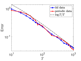
Figure 1. Convergence plot for EKI using periodic data and iid data.

5.2. Ergodic experiment: Dynamic solution operator

Our second experiment uses a static observation operator $\mathcal{O}$ but incorporates a dynamic solution operator $G_{t}$ for (1.6) using different realizations of the diffusion coefficient $a$. We again consider two different scenarios, but this time of iid and ergodic observation models.

We assume that we are in the scenario of Example 1.1, (iii), where the observation operator is fixed $\mathcal{O}=\mathcal{O}_{[x_{1}:x_{K}]}$ for fixed locations of observation $x_{1},\dots,x_{K}\in D$ and the diffusion coefficient is unknown. To be more precise, we assume that in general we have access to some statistical information about $a$ in form of a probability distribution $\pi$. For example, this information may come from a pre-stage Bayesian experiment. In many practical scenarios the explicit computation of $\pi$ or the generation of exact samples of $\pi$ is infeasible and for our ergodic observation model we assume that the information about the diffusion coefficient has been generated by a Markov chain Monte Carlo (MCMC) algorithm. As comparison we also consider the simplified setting, where one can generate iid samples of $\pi$.

5.2.1. Independent and identically distributed observation model

Firstly, we assume that there is access to a sample of iid realizations of $\pi$ denoted by $(a_{t}^{\mathrm{iid}})_{t\geq 0}$. The observations are then defined by

$$u_{t}=S_{t}z^{\ast}+w_{t}\,,$$

where $S_{t}=\mathcal{O}\circ G_{t}$ with $G_{t}=G_{a_{t}^{\mathrm{iid}}}$. Again, we make use of this model to construct our reference solution

$$z_{\mathrm{ref}}:=\arg\min_{z}\ J_{N}(z),\quad J_{N}(z):=\frac{1}{2N}\sum_{t=1}^{N}\|S_{t}z-u_{t}\|^{2}+\frac{\alpha}{2}\|z\|^{2}$$

for a large number of $N\gg 1$ iid observations. Similarly as before, we fix a regularization parameter of $\alpha=2$.

5.2.2. Ergodic observation model

Secondly, as discussed above we assume that the information about the diffusion coefficient comes from an ergodic Markov chain $(a_{t}^{\mathrm{e}})_{t\geq 0}$ with invariant distribution $\pi$. To be more precise, we assume that this information about the diffusion coefficient has been generated by an MCMC algorithm. The observation model is then defined by

$$u_{t}=S_{t}z^{\ast}+w_{t}\,,$$

where $S_{t}=\mathcal{O}\circ G_{t}$ with $G_{t}=G_{a_{t}^{\mathrm{e}}}$.

Let us now consider how we generate our correlated data. We consider a stationary distribution given as Gaussian distribution. In order to generate the Markov chain $(a_{t}^{\mathrm{e}})_{t\geq 0}$ with invariant distribution $\pi$, we implement a MCMC method, in particular the Metropolis-Hastings MCMC (MH-MCMC) algorithm.

We use the MH-MCMC method based on proposing moves using on a pre-conditioned Crank Nicholson (pCN) scheme of the form,

$$y^{\prime}=\sqrt{1-\beta^{2}}y+\beta\epsilon,\quad\epsilon\sim\mathcal{N}(0,\mathcal{C}),$$

with covariance structure defined as a Matérn covariance function, which is simulated through the KLE, as defined in (5.2). The proposal distribution is then of the form

$$y^{\prime}\sim\mathcal{N}((1-\beta^{2})y,\beta^{2}\mathcal{C}),$$

which uses an acceptance probability to either accepted or reject the proposed moves, defined as

$$\alpha_{\textrm{acc}}(y,y^{\prime})=\min\bigg{\{}1,\frac{\pi(y^{\prime})}{\pi(y)}\bigg{\}}\,.$$

For our numerical experiments we set $\beta=0.9$ of our proposal to ensure our acceptance rate is approximately $\alpha_{\mathrm{accep}}=0.234$, which is consistent with the “optimal” value for RWMH. When running our DEKI algorithm we again specify $J=50$ ensemble members where we place $T=1000$. Our groundtruth $z^{\ast}$ is again a realization of (5.2) with specific choices $(\ell,\nu)=(0.07,3.4)$. Figure 2 presents our generated groundtruth $z^{\ast}$ and the corresponding solution to the Darcy flow PDE. Our step size for the experiment is chosen again as $\eta_{t}=t^{-1}$. Our numerical experiments are shown in Figure 3 where we, as before, observe the theoretical rates from Theorem 2.1 and Corollary 2.2. Interestingly what we see is that at the beginning of the learning process, the ergodic data is slower as the initialization of the MCMC process induces a burn-in period. To allow for this we set the initialization as normal distribution with mean $\mu_{\textrm{mean}}=3$. However after roughly 200 iterations, we see that it does eventually converge with the correct theoretical rate.

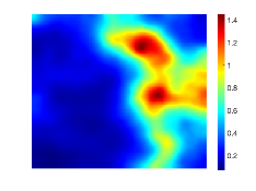
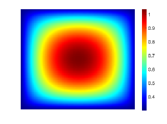
Figure 2. left: Plot of our random field representation of $z^{\ast}$ based on the KLE (5.2). right: Solution of the PDE (1.6).

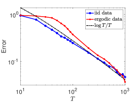
Figure 3. Convergence plot for EKI using ergodic data and iid data.

6. Conclusion

Within the field of inverse problems, it is common to learn unknown parameters from noisy data where the forward operator is static. In this work we consider the setting where instead we aim to learn parameters where there is a time-dependent forward operator, i.e. the forward model is dynamic. We consider this in the setting of an optimizer for black-box inverse problems, which is the EKI. Our new algorithm, which we refer to as dynamic-EKI, is introduced in a modified setting where we assume a linear least squares problem with the addition of Tikhonov regularization. A number of important results are derived which include a moment bound and ensemble collapse result, and our main result which is a convergence analysis. Our results apply to different data cases such as (i) iid data, (ii) ergodic data and (iii) periodic data. Numerical experiments are conducted on a toy model based on a linear elliptic PDE-constrained optimization problem using the 2D Darcy flow model. Our experiments demonstrate and verify our theoretical findings.

We conclude this article with a number of potentially useful directions to enhance our work. These are summarized below.

• Arguably the most important extension is related to theory, in terms of two aspects. The first being a non-linear analysis [11, 43], and the other being the extension to an infinite-dimensional analysis. Both works, in particular the first, are of significant challenge as there has been limited work, in general, for the linear case which we are able to provide analysis. The latter work is currently ongoing work by the authors.

• An obvious question is if this work could be extended to adaptive choice of $\alpha_{t}$? For example one could consider bilevel learning [12], as well as other adaptive Tikhonov strategies [41].

• Another interesting direction to consider is exploiting this framework in the continuous-time version. In the context of continuous dynamics with ergodic data, one could perhaps using Langevin based ideas from MALA and HMC, as examples for advanced proposals within MH methods.

• A final consideration could be on the influence of either variance inflation or localization [6, 7, 37, 38]. These techniques are known to help improve EKI. In the context of dynamic-EKI, it may also be the case where one could attain improved rates of convergence.

References

- [1] H. Albers and T. Kluth. Time-dependent parameter identification in a Fokker-Planck equation based magnetization model of large ensembles of nanoparticles. Arxiv preprint, arxiv:2307.03560, 2023.
- [2] M. Benning and M. Burger. Modern regularization methods for inverse problems, Acta Numerica, 27, 2018.
- [3] D. Blömker, C. Schillings, P. Wacker. A strongly convergent numerical scheme from ensemble Kalman inversion, SIAM J. Numerical Analysis, 56(4), 2018.
- [4] D. Blömker, C. Schillings, P. Wacker and S. Weissmann. Well posedness and convergence analysis of the ensemble Kalman inversion, Inverse Problems, 2019.
- [5] D. Blömker, C. Schillings, P. Wacker and S. Weissmann. Continuous Time Limit of the Stochastic Ensemble Kalman Inversion: Strong Convergence Analysis, SIAM Journal on Numerical Analysis, 60(6), 2019.
- [6] N. K. Chada. Analysis of hierarchical ensemble Kalman inversion. arXiv preprint arXiv:1801.00847, 2018.
- [7] N. K. Chada, Y. Chen, D. Sanz-Alonso. Iterative ensemble Kalman methods: A unified perspective with some new variants. Foundations of Data Science, 3(3), 331–369, 2021.
- [8] N. K Chada, M. A. Iglesias, L. Roininen, and A. M. Stuart. Parameterizations for ensemble Kalman inversion. Inverse Problems, 34(5):055009, 2018.
- [9] N. K. Chada, C. Schillings, and S. Weissmann. On the incorporation of box-constraints for ensemble Kalman inversion. Foundations of Data Science, 1(2639-8001 2019 4 433):433–456, 2019.
- [10] N. K. Chada, A. M. Stuart and X. T. Tong. Tikhonov regularization within ensemble Kalman inversion. SIAM Journal on Numerical Analysis, 58(2):1263–1294, 2020.
- [11] N. K. Chada and X. T. Tong. Convergence acceleration of ensemble Kalman inversion in nonlinear settings. Math. of Comp., 91(335), 1247–1280, 2022.
- [12] N. K. Chada, C. Schillings, X. T. Tong and S. Weissmann. Consistency analysis of bilevel data-driven learning in inverse problems. Communications in Mathematical Sciences, 20(1), 123–164, 2022.
- [13] N. Chen, A. J. Majda and X. T. Tong. Information barriers for noisy Lagrangian tracers in filtering random incompressible flows. Nonlinearity, 27,2133–2163, 2014.
- [14] Z. Ding and Q. Li. Ensemble Kalman sampler: mean-field limit and convergence analysis, SIAM J. Math. Anal., 53(2), 1546–1578, 2021.
- [15] G. Evensen. Data Assimilation: The Ensemble Kalman Filter. Springer, 2009.
- [16] G. Evensen. The ensemble Kalman filter: Theoretical formulation and practical implementation. Ocean dynamics, 53(4):343–367, 2003
- [17] M. Even. Stochastic gradient descent under Markovian sampling schemes. Proceedings of the 40th International Conference on Machine Learning, PMLR 202:9412–9439, 2023.
- [18] A. Garbuno-Inigo, F. Hoffmann, W. Li and A. M. Stuart, Gradient structure of the ensemble Kalman flow with noise. SIAM J. Applied Dynamical Systems, 19(1), 412–441, 2020.
- [19] M. Hanu, J. Latz and C. Schillings. Subsampling in ensemble Kalman inversion. Inverse Problems, 39(9) 2023.
- [20] M. A. Iglesias. A regularising iterative ensemble Kalman method for PDE-constrained inverse problems. Inverse Problems, 32, 2016.
- [21] M. A. Iglesias, K. J. H. Law and A. M. Stuart. ensemble Kalman methods for inverse problems. Inverse Problems, 29, 2013.
- [22] M. A. Iglesias and Y. Yang. Adaptive regularisation for ensemble Kalman inversion. Inverse Problems, 37 025008, 2021.
- [23] M. Iglesias, M. Park and M. V. Tretyakov. Bayesian inversion in resin transfer molding. Inverse Problems, 34(10), 105002, 2019.
- [24] B. Kaltenbacher. All-at-once versus reduced iterative methods for time dependent inverse problems. Inverse Problems, 33, p. 064002, 2017.
- [25] B. Kaltenbacher, T. Schuster, and A. Wald. Time-dependent Problems in Imaging and Parameter Identification. Springer International Publishing, Cham, 2021.
- [26] R. Klein, T. Schuster, and A. Wald. Sequential subspace optimization for recovering stored energy functions in hyperelastic materials from time-dependent data. In: Time-dependent Problems in Imaging and Parameter Identification, 2021.
- [27] G. Li and A. C. Reynolds. Iterative ensemble Kalman filters for data assimilation. SPE J 14 496-505, 2009
- [28] A. Majda and X. Wang. Non-linear Dynamics and Statistical Theories for Basic Geophysical Flows, Cambridge University Press, 2006.
- [29] S. P. Meyn and R. L. Tweedie. Markov Chains and Stochastic Stability. Cambridge University Press, 1993.
- [30] T.T.N. Nguyen. Landweber–Kaczmarz for parameter identification in time-dependent inverse problems: all-at-once versus reduced version. Inverse Problems, 35, 035009, 2019.
- [31] E. Somersalo, M. Cheney and D. Isaacson. Existence and Uniqueness for Electrode Models for Electric Current Computed Tomography, SIAM J. Appl. Math., 52, 1023-1040, 1992.
- [32] C. Schillings and A. M. Stuart. Analysis of the ensemble Kalman filter for inverse problems. SIAM J. Numer. Anal., 55(3):1264–1290, 2017.
- [33] A. M. Stuart. Inverse problems: A Bayesian perspective. Acta Numerica, Vol. 19, 451-559, 2010.
- [34] T. Sun and D. Li. Decentralized Markov chain gradient descent. arxiv preprint, arXiv:1909.10238, 2019.
- [35] T. Sun, Y. Sun and W. Yin. On Markov chain gradient descent. 32nd Conference on Neural Information Processing Systems, 2018.
- [36] A. Tarantola. Inverse Problem Theory and Methods for Model Parameter Estimation. Elsevier, 1987.
- [37] X. T. Tong, A. J. Majda and D. Kelly. Nonlinear stability of the ensemble Kalman filter with adaptive covariance inflation. Commun. Math. Sci., 14(5):1283–1313, 2016.
- [38] X. T. Tong and M. Morzfeld Localized ensemble Kalman inversion Inverse Problems, 32(1) 064002, 2023.
- [39] T. van Leeuwen and F. J. Herrmann. A penalty method for PDE-constrained optimization in inverse problems. Inverse Problems, 39(6) 015007, 2016.
- [40] P. Wang, Y. Lei, Y. Ying and D-X. Zhou. Stability and generalization for Markov Chain stochastic gradient methods. In Advances in Neural Information Processing Systems, 2022.
- [41] S. Weissmann, N. K. Chada, C. Schillings and X. T. Tong. Adaptive Tikhonov strategies for ensemble Kalman inversion. Inverse Problems, 38(4), 2022.
- [42] A. Majda and X.T. Tong, Intermittency in turbulent diffusion models with a mean gradient Nonlinearity, 28(11), 2015.
- [43] S. Weissmann Gradient flow structure and convergence analysis of the ensemble Kalman inversion for nonlinear forward models Inverse Problems, 38(10), 2022.