Low-Tubal-Rank Tensor Recovery via Factorized Gradient Descent
Abstract
This paper considers the problem of recovering a tensor with an underlying low-tubal-rank structure from a small number of corrupted linear measurements. Traditional approaches tackling such a problem require the computation of tensor Singular Value Decomposition (t-SVD), that is a computationally intensive process, rendering them impractical for dealing with large-scale tensors. Aim to address this challenge, we propose an efficient and effective low-tubal-rank tensor recovery method based on a factorization procedure akin to the Burer-Monteiro (BM) method. Precisely, our fundamental approach involves decomposing a large tensor into two smaller factor tensors, followed by solving the problem through factorized gradient descent (FGD). This strategy eliminates the need for t-SVD computation, thereby reducing computational costs and storage requirements. We provide rigorous theoretical analysis to ensure the convergence of FGD under both noise-free and noisy situations. Additionally, it is worth noting that our method does not require the precise estimation of the tensor tubal-rank. Even in cases where the tubal-rank is slightly overestimated, our approach continues to demonstrate robust performance. A series of experiments have been carried out to demonstrate that, as compared to other popular ones, our approach exhibits superior performance in multiple scenarios, in terms of the faster computational speed and the smaller convergence error.
Index Terms:
low-tubal-rank tensor recovery, t-SVD, factorized gradient descent, over parameterization.I Introduction
Tensors are higher-order extensions of vectors and matrices, capable of representing more complex structural information in high-order data. In fact, many real-world data can be modeled using tensors, such as hyperspectral images, videos, and sensor networks. These data often exhibit low-rank properties, and hence, many practical problems can be transformed into low-rank tensor recovery problems, as exemplified by applications such as image inpainting[65, 66, 67], image and video compression[3, 4], background subtraction from compressive measurements [5, 6], computed tomography[7] and so on. The goal of low-rank tensor recovery is to recover a low-rank tensor from the noisy observation
| (1) |
where is the unknown noise. This model can be concisely expressed as
where denotes a linear compression operator and , . When the target tensor is low-rank, a straightforward method to solve this model is rank minimization
| (2) |
where denotes the noise level, rank() is the tensor rank function.
However, there are still numerous ambiguities in the numerical algebra of tensors. A primary concern arises from the existence of various tensor decomposition methods, each linked to its corresponding tensor rank, e.g., CONDECOMP/PARAFAC decomposition (CP) [8, 64], Tucker decomposition [9], tensor Singular Value Decomposition (t-SVD)[1], among others. The CP decomposition involves decomposing a tensor into the sum of several rank-1 out product of vectors. Hence, the CP rank corresponds to the number of rank-one decompositions employed in this factorization. While CP-rank aligns intuitively with matrix rank, its determination is rendered challenging due to its status as a NP-hard problem. Tucker decomposition initially involves unfolding the tensor into matrices along distinct modes, followed by decomposing the tensor into the product of a core tensor and the matrices corresponding to each mode. The Tucker rank corresponds to the rank of the matrices obtained after unfolding the tensor along different modes. Therefore, its rank computation is relatively straightforward, yet it cannot leverage the relationships between modes. Leveraging tensor-tensor product (t-product), Kilmer et al. [1] introduced the t-SVD and its associated tensor rank, referred to as tubal-rank. Specifically, the t-SVD transforms a three-order tensor into the frequency domain. Subsequently, SVD is applied to each frontal slice, followed by an inverse transformation. This process yields three factor tensors, which is similar to matrix SVD. The advantage of t-SVD is that it has a theory similar to the Eckart-Young Theorem for matrices to guarantee its optimal low-tubal-rank approximation. Furthermore, the tubal-rank provides a more effective description of the low-rank property of tensors. Consequently, our emphasis in this paper lies in low-tubal-rank tensor recovery (LTRTR) under t-SVD framework.
Within the framework of t-SVD, numerous studies have already been conducted on low-rank tensor recovery. Since the rank constraint in problem (2) is NP-hard, Lu et.al[11] proposed a t-product induced tensor nuclear norm (TNN). Hence, the optimization (2) can be loosed into a convex optimization problem [11]
However, tensor nuclear norm minimization methods necessitate the computation of t-SVD decomposition, which is an extremely time-consuming process. As the dimensions of the tensor become large, the computational overhead and storage space associated with these methods becomes increasingly prohibitive.
| t-SVD methods | operator | recovery theory | convergence rate | iteration complexity | over rank |
| TNN [10] | measurement | ✓ | ✗ | ||
| IR-t-TNN [12] | measurement | ✓ | sub-linear | ||
| RTNNM [2] | measurement | ✓ | ✗ | ||
| TCTF [15] | projection | ✗ | ✗ | ✗ | |
| HQ-TCSAD [29] | projection | ✗ | ✗ | ✗ | |
| UTF[30] | projection | ✗ | ✗ | ✓ | |
| DNTC&FNTC[20] | projection | ✗ | ✗ | ✓ | |
| Ours | measurement | ✓ | linear sub-linear | ✓ |
However, similar challenge is also present in low-rank matrix recovery. In the realm of low-rank matrix recovery, numerous endeavors have focused on decomposing large low-rank matrices into smaller factor matrices to reduce computational complexity, which is called the Burer-Monteiro (BM) method [23]. Consequently, it is natural that we extend this paradigm to tensors as tensor BM factorization. To address these challenges, we propose the utilization of FGD for solving LTRTR problem. Specifically, we decompose a symmetric positive semi-definite (T-PSD) tensor as , leading to the formulation of the following optimization problem
| (3) |
where denotes the t-product (see Definition 2.4) and denotes the transpose of . It is noteworthy that in this context, precise knowledge of the exact tubal-rank of the original tensor is not necessary; rather, we only require that , that’s over rank or over-parameterized situation. This condition proves to be more practical in real-world applications. Such an optimization problem can be efficiently solved using FGD, thereby significantly reducing computational costs. In Table I, we compare our method in detail with other t-SVD based methods. In the case of exact rank, FGD demonstrates linear convergence, surpassing other methods; in the over rank situation, FGD exhibits sub-linear convergence similar to IR-t-TNN. However, it is important to highlight that the iteration complexity of FGD is significantly lower than IR-t-TNN. In summary, our method is an general and efficient approach with theoretical underpinnings.
I-A Main contributions
The main contributions of this article can be summarized as follows:
-
•
In response to the high computational complexity associated with existing methods, we propose an effective and efficient approach based on tensor BM factorization for LTRTR. Our approach involves decomposing a large tensor into the t-product of two smaller tensors, followed by the application of FGD to address the recovery problem. This method effectively reduces computational overhead.
-
•
We provide theoretical guarantees for the recovery performance of the FGD method under noiseless, noisy, exact rank and over rank situations. In the absence of noise, our method ensures exact recovery, while in the presence of noise, it converges to a deterministic error. Furthermore, our theory ensures that, the FGD method maintains favorable performance even in the over rank scenario.
-
•
The experimental outcomes affirm that our method exhibits not only the fastest convergence to the true value in noise-free scenarios but also converges to the minimum error bound in the presence of noise. Noteworthily, experiments results indicate that even when the tubal-rank is slightly overestimated, the target tensor can still be accurately recovered.
I-B Related work
I-B1 Low rank tensor recovery with t-SVD framework
Early works on LTRTR primarily focused on utilizing convex methods. Lu et al. [37] proposed a novel tensor nuclear norm based on reversible linear transformations and utilized nuclear norm minimization to solve the low-rank tensor completion problem. Zhang et al.[2] pioneered the definition of the Tensor Restricted Isometry Property (T-RIP), providing proof that, the robust recovery of any third-order tensor is attainable with the help of T-RIP. Furthermore, Zhang et al.[36] demonstrated that, under certain conditions on the number of measurements, linear maps satisfies the T-RIP conditions exist. In addressing the LTRTR problem under binary measurements, Hou et al.[18] introduced two t-SVD-based approaches, ensuring the successful recovery of tensors from binary measurements. While convex methods for low-rank tensor recovery offer superior experimental performance , their computational demands become prohibitive as the scale of data increases.
In recent years, numerous efforts have been dedicated to solving the LTRTR problem using non-convex methods. These works can be primarily classified into two categories: one that transforms convex constraints into non-convex constraints, and another that decomposes large tensors into smaller tensors. Kong et al. [38] introduced a new tensor Schatten-p norm regularizer and proposed an efficient algorithm to solve the resulting nonconvex problem. However, their method does not offer rigorous recovery guarantees. Based on t-product induced tensor nuclear norm, weighted tensor nuclear norm [39] and partial sum of tubal nuclear norm [40] were proposed for solving low-rank tensor completion problem. In addition, Wang et al.[12] proposed an general non-convex method named IR-t-TNN for LTRTR. Nonetheless, their method still involves computing t-SVD, leading to a substantial computational workload.
Another category of non-convex methods, specifically, the decomposition-based approach which decomposes large tensors into smaller tensors, has drawn a lot of attenton. Zhou et al.[15] proposed an efficient algorithm for tensor completion based on tensor factorization avoiding the calculation of t-SVD. He et al. [29] proposed an robust low-tubal-rank tensor completion method via alternating steepest descent method and tensor factorization. However, these two approaches typically necessitate knowledge of the true rank of the target tensor, a requirement that is often challenging to meet in practical situations. Some works have addressed and improved upon this issue by considering scenarios where the true rank remains unknown. Du et al. [30] introduced a Unified Tensor Factorization (UTF) method for addressing the low-tubal-rank tensor completion problem. Their approach eliminates the necessity of knowing the true tubal-rank of the original tensor. Jiang et al.[20] based on their self-defined tensor double nuclear norm and Frobenius/nuclear hybrid norm, decomposed tensors into two factor tensors and proposed corresponding solving algorithms for tensor completion problem. However, as stated in Table I, these two methods lack theoretical recovery guarantees.
I-B2 Low rank tensor recovery with other decomposition frameworks
For other decomposition frameworks, a significant amount of research has been devoted to addressing the low-rank tensor recovery problem. For CP decomposition, there are various methods, including but not limited to: sum-of-squares method for exact and noisy [41] tensor completion [42]; vanilla gradient descent with nearly linear time[28, 43]; alternating minimization with linear convergence[44, 45]; spectral methods [46, 47, 48]; automic norm minimization [49, 50]. In addition to CP decomposition, there is a substantial body of work focused on solving low-rank tensor recovery problems using Tucker decomposition, including but not limited to: nuclear norm minimization by unfolding tensor [35, 34, 51]; spectral methods [52, 53]; gradient methods on manifold optimization [56, 54, 55, 26, 21]. For tensor train decomposition[58] and tensor ring decomposition [63], the methods for low rank tensor recovery involve: parallel matrix factorization [60, 61, 62], Riemannian preconditioned methods[59, 57], to name a few. Due to the differences in tensor decomposition frameworks, we won’t delve into detailed explanations of these methods.
II Notations and preliminaries
In this paper, the terms scalar, vector, matrix, and tensor are represented by the symbols , x, and respectively. The inner product of two tensors, and , is defined as . The tensor Frobenius norm is defined as . The spectral norm of matrices and tensors are denoted by . Moreover, denotes the -th frontal slice of and denotes the -th frontal slice of while is the Fast Fourier Transform (FFT) of along the third dimension. In Matlab, we have and .
Definition II.1 (Block diagonal matrix [1])
For a three-order tensor , we denote as a block diagonal matrix of , i.e.,
Definition II.2 (Block circulant matrix [1])
For a three-order tensor , we denote as its block circulant matrix, i.e.,
Definition II.3 (The fold and unfold operations [1])
For a three-order tensor , we have
Definition II.4 (T-product[1])
For , , the t-product of and is , i.e.,
Definition II.5 (Tensor conjugate transpose[1])
Let , and its conjugate transpose is denoted as . The formation of involves obtaining the conjugate transpose of each frontal slice of , followed by reversing the order of transposed frontal slices 2 through .
Definition II.6 (Identity tensor[1])
The identity tensor, represented by , is defined such that its first frontal slice corresponds to the identity matrix, while all subsequent frontal slices are comprised entirely of zeros. This can be expressed mathematically as:
Definition II.7 (Orthogonal tensor [1])
A tensor is considered orthogonal if it satisfies the following condition:
Definition II.8 (F-diagonal tensor [1])
A tensor is called f-diagonal if each of its frontal slices is a diagonal matrix.
Theorem 1 (t-SVD [1, 10])
Let , then it can be factored as
where , are orthogonal tensors, and is a f-diagonal tensor.
Definition II.9 (Tubal-rank [1])
For , its tubal-rank as rank is defined as the nonzero singular tubes of , where is the f-diagonal tensor from the t-SVD of . That is
Definition II.10 (Tensor column space [25, 24])
Consider a tensor with a tubal-rank of . Let denote the t-SVD of . The column space of is spanned by , where the first columns of each consist of the first columns of , with the remaining columns being zeros.
Definition II.11 (Tensor spectral norm [10])
For , its spectral norm is denoted as
Definition II.12 (Tensor Restricted Isometry Property, T-RIP [2])
A linear mapping, denoted as , is said to satisfy the T-RIP of order with tensor Restricted Isometry Constant (t-RIC) if is the smallest value such that
holds for all tensors with a tubal-rank of at most .
Definition II.13 (Tensor condition number)
The condition number of a tensor is defined as
where denote the singular values of . In this paper, we abbreviate and as and , and denote for simplicity.
Definition II.14 (T-positive semi-definite tensor (T-PSD) [19])
For any symmetric , is said to be a positive semi-definite tensor, if we have
for any .
III Main results
In this context, we initially present an detailed exposition on low-tubal-rank tensor BM factorization, followed by an analysis of its convergence rate and estimation error. Finally, we provide the algorithm’s computational complexity.
III-A Formulation of tensor BM factorization
As discussed in Section 1, the target of LTRTR is to recover a low-tubal-rank tensor from the following noisy observations
where we assume is the Gaussian noise, rank and are symmetric tensors with sub-Gaussian entries. Many traditional methods for LTRTR require computationally expensive t-SVD. When the tensor dimensions are large, these methods become impractical. Therefore, addressing this issue, we aim to devise an efficient and provable method for LTRTR. Drawing inspiration from the Burer-Monteiro method[23], a commonly used approach in low-rank matrix recovery, where a large matrix is decomposed as , , we seek to extend this concept to the decomposition of large tensors into smaller factor tensors.
Our first step involves investigating a tensor factorization method akin to the Burer-Monteiro method, which focus on symmetric positive semi-definite matrix. For simplicity, we consider the case where the tensor is T-PSD. The more general scenarios can be extended based on our work. Subsequently, our task is to establish the proof that any T-PSD tensor can be decomposed into . To accomplish this, we first introduce the tensor eigenvalue decomposition based on t-SVD framework, which is crucial for our analysis.
Theorem 2
(T-eigenvalue decomposition [19]) Any symmetric could be decomposed into
where is an orthogonal tensor and is a f-diagonal tensor with all diagonal entries of being the T-eigenvalues of . Note that the T-eigenvalues of are eigenvalues of . Especially , if is a T-PSD tensor, then all T-eigenvalues of are non-negative.
Based on T-eigenvalue decomposition, we derive the following lemma.
Lemma 1
For any symmetric T-PSD tensor with tubal-rank , it can be decomposed into , where .
Then we factorize a T-PSD tensor into , and obtain the following optimization problem:
| (4) |
where , that means we do not need to accurately estimate the tubal-rank of . A classical approach to optimizing this problem involves obtaining an initial point close to the , followed by the application of FGD for local convergence, which is shown in Algorithm 1.
Regarding the initialization, we make the following assumption.
Assumption 1
| (5) |
Noting that this initialization can be obtained by some spectral methods in matrices [32, 31, 33] since we have the unique correlation
which establishes a connection between the spectral norm of matrix and the tensor spectral norm.
With this initialization assumption, we perform FGD to solve problem (4),
| (6) |
III-B Main Theorem
We have conducted an analysis of the convergence and convergence error of FGD in four scenarios: noise-free/existence of noise, exact rank/over rank. Below, we present the direct results of our analysis.
Theorem 3
Assume that , and set step size , where , and we have a good initialization as Assumption 1 with , then the ensuing claims hold with a probability of at least :
(a) when and , we have
(b) when and , we have
for any , where ;
(c) when and , we have
(d) when and , we have
for any .
Remark III.1
In the case of exact rank (), regardless of the presence of noise, the convergence rate of FGD is linear. Conversely, in the over rank scenario (), irrespective of the existence of noise, the convergence rate of FGD is sub-linear. These findings are consistent with the experimental results presented in Section 4.
Remark III.2
Even in the presence of noise, whether over-parameterized or not, the term remains constant. Regarding the recovery error , we have due to the inequality . Therefore, in the case of , we achieve the minimal recovery error. When slightly exceeds , the impact of over rank on the recovery error is still acceptable, due to the square root factor.
Remark III.3
It is noteworthy that, among the numerous works on LTRTR, we provide, for the first time, both the convergence rate and convergence error of this problem. Convex methods such as TNN [10] and RTNNM [2] only offer guarantees for convergence error without specifying the convergence rate. On the other hand, non-convex methods, such as the IR-t-TNN proposed by Wang et al. [12], provide a rough convergence rate analysis based on the Kurdyka-Lojasiewicz property. For more detailed comparison, please refer to Table I.
III-C Population-sample analysis
According to the T-eigenvalue decomposition, we decompose as
where , , Here, and represent orthonormal tensors that are complementary, denoted as . Consequently, for any , it can be consistently factorized as follows:
where and . Then we have
As approaches infinity, if we have converges to , and , and converge to 0, then approximates to .
Then we consider the gradient descent
Noting that denotes the population gradient descent while the original gradient descent denotes the sample gradient descent. Therefore, in the analysis of local convergence, we follow the typical population-sample analysis[14, 13].
III-C1 Population analysis
For term , we have
where we define
It is worth noting that is, in fact, the gradient descent method applied to optimization problem
| (7) |
Then we have the following Lemma:
Lemma 2
Suppose that we have the same settings as Theorem 3, for the case , we have
When , we have
where the bounds for and remain the same as (a) and (b).
Remark III.4
Lemma 2 indicates that under the over-parameterized scenario, the slowest convergence is observed in , which converges at a sub-linear rate, leading to sub-linear convergence in the over-parameterized setting. Conversely, in the exact rank scenario, exhibits the fastest convergence, while converges at the slowest rate in this context. However, it is noteworthy that all cases exhibit linear convergence rates in the exact rank scenario.
We present an additional Lemma that establishes a connection between the population case and the sample case.
Lemma 3
Suppose we have the same settings as Theorem 3, then we have
Building upon these two Lemmas, we proceed with the analysis under the finite sample scenario.
III-C2 Finite sample analysis
For term , we can control it by the T-RIP and concentration inequalities.
Lemma 4
Suppose that we have the same settings as Theorem 3, then we have
(a)
holds with probability at least ;
(b)
holds with probability at least . Furthermore, we have .
Based on the aforementioned lemmas, we can bound by the following Lemma.
Lemma 5
Define . Suppose we have the same settings as Theorem 3, then we have the following hold with high probability:
(a) noiseless and exact rank case,
(b) noisy and exact rank case,
(c) noiseless and over rank case,
(d) noisy and over rank case,
where we define .
Remark III.5
Lemma 5 reveals that under the exact rank scenario, irrespective of the presence of noise, converges at a linear rate. On the other hand, in the over-parameterized scenario, regardless of the noise level, converges at a sub-linear rate.
III-D Main proofs
To prove Theorem 3, it is necessary to establish all the lemmas employed in this paper. Due to space constraints, we provide the proof of only Lemma 5 here, as it is most relevant to Theorem 3. The proofs of other lemmas are deferred to the supplementary materials.
III-D1 Proof of Lemma 5
To bound , it is imperative to individually bound the three components , and .
Upper bounds for :
By the definitions of and , we have
For we have
For , we have
Note that the spectral norm of the terms and are the same; and are the same; and are the same, which can be bounded as follows:
For term , we have
| (8) | ||||
Putting these results together, we obtain
where we using the fact that
and .
Consider the noiseless case, we have
Upper bounds for :
By the definitions of and , we have
For , we have
For , we have
Direct application of inequalities with operator norms leads to
For term , we can bound it like term in equation (8):
Collecting all these results, we obtain
For the noiseless case, we have
| (9) |
Upper bounds for :
By the definition of , we have
For , we can bound it like term in equation (8):
Collecting all these results together, we obtain
where we take for notation convenience. Then we define , and with some algebraic manipulations, we have
for the noisy and over rank case. Considering the noiseless and over rank case, we obtain
For the exact parameterization case, we have
from Lemma 2. Then we have
for the noisy case. For the noiseless case, we have
| (10) |
After bounding each of the three components , and separately, we can proceed to establish bounds for .
Upper bounds for :
(a) For the noiseless and exact rank case, we have
Then we obtain
(b) For the noisy and exact rank case, we have
| (11) | ||||
leading to the result
(c) For the noiseless and over rank case, we have
| (12) | ||||
leading to the result
(d) For the noisy and over rank case, we have
| (13) | ||||
where and . Then we obtain
| (14) |
III-D2 Proof of Theorem 3
Prior to establishing Theorem 3, we provide a lemma that serves to establish a connection between and as outlined in Lemma 5.
Lemma 6
Suppose that we have the same settings as Theorem 3, define , we have
Under the assumptions of Theorem 3, Lemma 5 holds. Therefore, based on Lemma 5, we proceed to prove Theorem 3. Given that Lemma 5 provides the convergence rate and convergence error of , we can establish the convergence properties of by utilizing the relationship . Thus, transforming the results of Lemma 5 using this relationship is sufficient to demonstrate Theorem 3.
Proof of claim (a)
We have
from Lemma 5. Subsequently, it is straightforward to obtain
where the last inequality using the fact that . And then we obtain
follows from the fact that
Proof of claim (b)
We have
form Lemma 5. For simplicity, we denote . Then we can derived that for , leading to the result that for , we have
Proof of claim (c)
We have
from Lemma 5. We claim that holds for any . This holds true in the case of . Then we assume that holds and prove it still holds when . For , we have
Therefore we obtain holds for any and . Then we utilize the fact that to derive
Proof of claim (d):
Firstly we have
from Lemma 5. We claim that holds for any , which is similar to claim (c). Therefore, for number of iterations, , leading to the result
III-E Complexity analysis
Here, we analyze the time complexity of FGD. For FGD, the computational workload per iteration primarily focuses on two steps: the FFT of three order tensors and t-product. The computational complexity of performing a t-product between and is denoted as . The computational complexity for calculating the FFT is denoted as . Combining the computational complexities of these two steps, we obtain the overall computational complexity per iteration for FGD, denoted as . As for the TNN method[10], its computational complexity is denoted as . And for the complexity of other methods, please refer to Table I. In comparing these methods, it is evident that our approach fully leverages the low-rank structure of the data, thereby effectively reducing the computational complexity.
IV Numerical experiments
We conduct a various experiments to verify our theoretical results. We first conducte two sets of experiments to validate the results of Lemmas 3 and 6. Then we compare our method with a convex method TNN[10] and a non-convex method IR-t-TNN[12] in the noiseless and noisy case. The experimental results indicate that our methodology not only showcases the highest computational speed in both noisy and noiseless scenarios but also attains minimal errors in the presence of noise. It is noteworthy that, even when the tubal-rank estimation for FGD is slightly higher, it still ensures excellent recovery performance. Our experiments were conducted on a laptop equipped with an Intel i9-13980HX processor (clock frequency of 2.20 GHz) and 64GB of memory, using MATLAB 2022b software.
We generate the target tensor with by , where the entries of are i.i.d. sampled from a Gaussian distribution . The entries of measurement tensor are i.i.d. sampled from a Gaussian distribution . The entries of noise s are i.i.d. sampled from a Gaussian distribution . The parameters of TNN, IR-t-TNN and FGD are fine-turned for the best result.
IV-A Verify the convergence rate
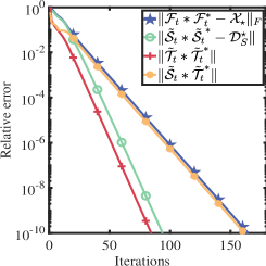
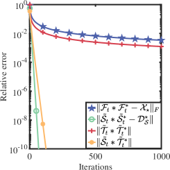
For the results of Lemma 2, we conducted two sets of experiments to validate the convergence rates under the scenarios of exact rank and over rank. As depicted in Figure 1 (a) and (b), it is evident that under the exact rank scenario, convergence occurs at a linear rate. Conversely, in the over rank scenario, and exhibit sub-linear convergence, with determining the rate of convergence for . Meanwhile, and converge at a linear rate in the over rank scenario.
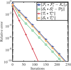
Regarding Lemma 5, we conducted two sets of noise-free experiments to verify the convergence rates under the scenarios of exact rank and over rank. As illustrated in Figure 1 (c) and (d), it is evident that under the exact rank scenario, convergence is linear, while under the over rank scenario, convergence is sub-linear. In comparison to Lemma 3, in the over-parameterized scenario, still determines the convergence of . However, unlike Lemma 2, under the over-parameterized scenario, both and exhibit sub-linear convergence, primarily influenced by .
IV-B Noiseless case
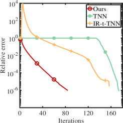
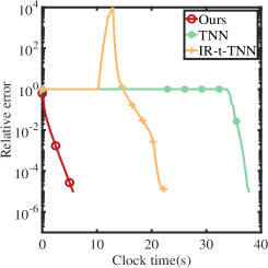
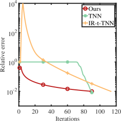
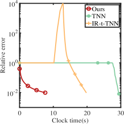
For the noiseless scenario, we conducted two sets of experiments comparing the recovery performance and computational efficiency of FGD, TNN, and IR-t-TNN under exact rank and over rank situations. From Figure 1, it can be observed that, under exact rank () situation, all three methods can ensure exact recovery. It is noteworthy that our approach achieves a linear convergence rate with minimal computational cost, consistent with our theoretical expectations. In the case of over rank (), our method exhibits sub-linear convergence but still guarantees convergence to a small relative error within a relatively short time. Furthermore, when the error reaches 0.01, the number of iterations required by our method and TNN is comparable, but the computation time for our method is significantly smaller than that for TNN, indicating the lower computational complexity of each step in our approach.
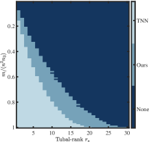
Additionally, we investigated the phase transition phenomena of FGD and TNN under different tubal-rank and the number of measurements . The IR-t-TNN algorithm, requiring a larger number of measurements, exhibits relatively poor performance in this experiment; hence, it is not included in the comparison. We set , . We vary between and , and vary between 1 and 30. For each pair of , we conducted 10 repeated experiments. In each experiment, we set the maximum number of iterations to 1000, and when the relative error , we considered to be successfully recovered. When the number of successful recoveries in 10 repeated experiments is greater than or equal to 5, we categorize that experimental set as a successful recovery, as illustrated in the graph. The deep blue region represents unsuccessful recoveries, while the other two colors represent the recovery outcomes of our method and TNN. It is evident that our method demonstrates significantly superior recovery performance compared to the TNN algorithm.
IV-C Noisy case
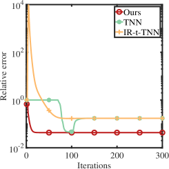
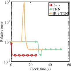
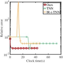
For the noisy scenario, we initially investigated the convergence rate and convergence error of FGD under both exact rank and over rank situations. From Figure 4, it is evident that FGD converges to the minimum relative error at the fastest rate, regardless of whether it is under exact rank or over rank conditions. In the case of exact rank, the convergence is linear, while in the over rank situation, it is sub-linear. In contrast, the final convergence errors for the other two methods are larger than that of FGD. Specifically, TNN converges initially to an error comparable to FGD and then diverges to a larger error. Additionally, it is observed that the computation time for IR-t-TNN is significantly smaller than that for TNN, demonstrating the efficiency of the non-convex method.
Then we conducted a series of experiments considering various values of , tubal-rank, and noise, with the experimental results presented in Tables II, III and IV. The stopping criteria for the TNN and IR-t-TNN algorithms were consistent with the original papers. The measurements number is set to be . For our algorithm, the termination point was set as , and . All experiments in the tables are repeated for 10 times.
Through these three sets of experiments, the following conclusions can be drawn:
-
•
In all scenarios of the three experiments, our FGD method achieved the minimum relative recovery error with the shortest computation time. For TNN and IR-t-TNN, their final recovery errors are very close. Additionally, the non-convex IR-t-TNN method has a significantly smaller computation time than the convex TNN method but is still much larger than our FGD method.
-
•
As the variance of the noise increases, the recovery errors for all three methods also increase. This aligns with the theoretical expectations of recovery error growth with higher noise levels.
-
•
As increases, the recovery errors for all three methods decrease. This is because the measurements number increases with the growth of , leading to a reduction in recovery errors, consistent with our theoretical expectations. Furthermore, with the increase in , the computation time for all three methods significantly increases.
-
•
As increases, the recovery errors for all three methods noticeably decrease. This is because the increase in results in an increase in the measurements number , consistent with theoretical expectations.
V Conclusion
This article proposes a non-convex LTRTR method based on a tensor type of Burer-Monteiro factorization, which significantly reduces computational and storage costs as compared with existing popular methods. We provide rigorous convergence guarantees and demonstrate that our method performs very well in both exact rank and over rank scenarios. The effectiveness and efficacy of the proposed method is further validated through a series of experiments. These presented finds offer new insights into LTRTR problems. In the future, we shall explore the following aspects:
-
•
Consider the recovery of over-parameterized tensors in asymmetric scenarios. Performing Research on asymmetric scenarios is more practical, and investigations in this context would be more meaningful.
-
•
Enhancing the convergence rate in the over rank situation. Our work demonstrated that FGD exhibits sub-linear convergence in the over rank situation, which is not good as the exact rank situation. Fortunately, the efficacy of employing small initialization [16, 27] or preconditioning techniques [22, 68] in expediting the convergence rate under over rank case has been substantiated for low-rank matrix recovery. Consequently, we contemplate the adoption of either small initialization or preconditioning techniques in our future work.
-
•
Explore LTRTR problem under ill-conditioned scenarios. It is known that the convergence rate of gradient descent is related to the condition number. Developing more efficient algorithms to enhance convergence rates under ill-conditioned scenarios is also an interesting avenue for exploration.
| TNN | IR-t-TNN | Ours | |||||
| error | time(s) | error | time(s) | error | time(s) | ||
| 30 | 0.3 | 0.0435 | 9.7994 | 0.0435 | 3.6334 | 0.0367 | 1.6395 |
| 0.5 | 0.0716 | 9.7912 | 0.0716 | 3.6764 | 0.0515 | 1.6696 | |
| 0.7 | 0.1021 | 9.7843 | 0.1021 | 3.6792 | 0.0702 | 1.7627 | |
| 50 | 0.3 | 0.0338 | 72.7788 | 0.0338 | 40.7706 | 0.0264 | 9.3127 |
| 0.5 | 0.0563 | 72.9363 | 0.0563 | 40.8795 | 0.0394 | 9.3879 | |
| 0.7 | 0.0790 | 72.6651 | 0.0790 | 40.6241 | 0.0533 | 9.449 | |
| 70 | 0.3 | 0.0285 | 396.4822 | 0.0285 | 235.2165 | 0.0216 | 30.8286 |
| 0.5 | 0.0475 | 396.2685 | 0.0475 | 234.6146 | 0.0328 | 30.854 | |
| 0.7 | 0.0664 | 394.6048 | 0.0664 | 233.6755 | 0.0443 | 30.1598 | |
| TNN | IR-t-TNN | Ours | |||||
| error | time(s) | error | time(s) | error | time(s) | ||
| 30 | 0.3 | 0.0589 | 7.4303 | 0.0589 | 3.2016 | 0.0429 | 1.0736 |
| 0.5 | 0.0984 | 7.3765 | 0.0984 | 3.1742 | 0.0515 | 1.1114 | |
| 0.7 | 0.1379 | 7.6562 | 0.1379 | 3.2838 | 0.0788 | 1.1631 | |
| 50 | 0.3 | 0.0456 | 56.4187 | 0.0456 | 33.5054 | 0.0309 | 6.0095 |
| 0.5 | 0.0760 | 55.8555 | 0.0760 | 33.1774 | 0.0443 | 6.0462 | |
| 0.7 | 0.1052 | 55.4032 | 0.1051 | 32.9169 | 0.0581 | 6.0301 | |
| 70 | 0.3 | 0.0382 | 308.8834 | 0.0382 | 184.8635 | 0.0249 | 18.1586 |
| 0.5 | 0.0641 | 307.2197 | 0.0641 | 183.9251 | 0.0368 | 18.7787 | |
| 0.7 | 0.0898 | 304.8521 | 0.0898 | 182.1509 | 0.0496 | 18.9125 | |
| TNN | IR-t-TNN | Ours | |||||
| error | time(s) | error | time(s) | error | time(s) | ||
| 30 | 0.3 | 0.1074 | 4.6677 | 0.1074 | 3.0643 | 0.0521 | 0.6427 |
| 0.5 | 0.1750 | 4.7164 | 0.1750 | 3.0935 | 0.0688 | 0.6671 | |
| 0.7 | 0.2533 | 4.657 | 0.2532 | 3.0787 | 0.0905 | 0.7101 | |
| 50 | 0.3 | 0.0838 | 36.054 | 0.0838 | 21.2458 | 0.0371 | 3.4385 |
| 0.5 | 0.1375 | 36.229 | 0.1374 | 21.4327 | 0.0504 | 3.5254 | |
| 0.7 | 0.1943 | 36.7619 | 0.1941 | 21.7769 | 0.0678 | 3.8409 | |
| 70 | 0.3 | 0.0693 | 199.7492 | 0.0692 | 109.3462 | 0.0297 | 10.0213 |
| 0.5 | 0.1178 | 200.8866 | 0.1177 | 110.0804 | 0.0425 | 10.5745 | |
| 0.7 | 0.1655 | 201.7875 | 0.1653 | 110.0439 | 0.05585 | 11.1467 | |
References
- [1] M. E. Kilmer and C. D. Martin, “Factorization strategies for third-order tensors,” Linear Algebra and its Applications, vol. 435, no. 3, pp. 641–658, 2011.
- [2] F. Zhang, W. Wang, J. Huang, J. Wang, and Y. Wang, “Rip-based performance guarantee for low-tubal-rank tensor recovery,” Journal of Computational and Applied Mathematics, vol. 374, p. 112767, 2020.
- [3] Y. Wang, L. Lin, Q. Zhao, T. Yue, D. Meng, and Y. Leung, “Compressive sensing of hyperspectral images via joint tensor tucker decomposition and weighted total variation regularization,” IEEE Geoscience and Remote Sensing Letters, vol. 14, no. 12, pp. 2457–2461, 2017.
- [4] R. G. Baraniuk, T. Goldstein, A. C. Sankaranarayanan, C. Studer, A. Veeraraghavan, and M. B. Wakin, “Compressive video sensing: Algorithms, architectures, and applications,” IEEE Signal Processing Magazine, vol. 34, no. 1, pp. 52–66, 2017.
- [5] W. Cao, Y. Wang, J. Sun, D. Meng, C. Yang, A. Cichocki, and Z. Xu, “Total variation regularized tensor rpca for background subtraction from compressive measurements,” IEEE Transactions on Image Processing, vol. 25, no. 9, pp. 4075–4090, 2016.
- [6] Z. Li, Y. Wang, Q. Zhao, S. Zhang, and D. Meng, “A tensor-based online rpca model for compressive background subtraction,” IEEE Transactions on Neural Networks and Learning Systems, 2022.
- [7] O. Semerci, N. Hao, M. E. Kilmer, and E. L. Miller, “Tensor-based formulation and nuclear norm regularization for multienergy computed tomography,” IEEE Transactions on Image Processing, vol. 23, no. 4, pp. 1678–1693, 2014.
- [8] J. D. Carroll and J.-J. Chang, “Analysis of individual differences in multidimensional scaling via an n-way generalization of “eckart-young” decomposition,” Psychometrika, vol. 35, no. 3, pp. 283–319, 1970.
- [9] L. R. Tucker, “Some mathematical notes on three-mode factor analysis,” Psychometrika, vol. 31, no. 3, pp. 279–311, 1966.
- [10] C. Lu, J. Feng, Z. Lin, and S. Yan, “Exact low tubal rank tensor recovery from gaussian measurements,” in Proceedings of the 27th International Joint Conference on Artificial Intelligence, 2018, pp. 2504–2510.
- [11] C. Lu, J. Feng, Y. Chen, W. Liu, Z. Lin, and S. Yan, “Tensor robust principal component analysis with a new tensor nuclear norm,” IEEE Transactions on Pattern Analysis and Machine Intelligence, vol. 42, no. 4, pp. 925–938, 2019.
- [12] H. Wang, F. Zhang, J. Wang, T. Huang, J. Huang, and X. Liu, “Generalized nonconvex approach for low-tubal-rank tensor recovery,” IEEE Transactions on Neural Networks and Learning Systems, vol. 33, no. 8, pp. 3305–3319, 2021.
- [13] J. Zhuo, J. Kwon, N. Ho, and C. Caramanis, “On the computational and statistical complexity of over-parameterized matrix sensing,” arXiv preprint arXiv:2102.02756, 2021.
- [14] S. Balakrishnan, M. J. Wainwright, and B. Yu, “Statistical guarantees for the em algorithm: From population to sample-based analysis,” The Annals of Statistics, vol. 45, no. 1, pp. 77–120, 2017.
- [15] P. Zhou, C. Lu, Z. Lin, and C. Zhang, “Tensor factorization for low-rank tensor completion,” IEEE Transactions on Image Processing, vol. 27, no. 3, pp. 1152–1163, 2017.
- [16] D. Stöger and M. Soltanolkotabi, “Small random initialization is akin to spectral learning: Optimization and generalization guarantees for overparameterized low-rank matrix reconstruction,” Advances in Neural Information Processing Systems, vol. 34, pp. 23 831–23 843, 2021.
- [17] H. Wang, J. Peng, W. Qin, J. Wang, and D. Meng, “Guaranteed tensor recovery fused low-rankness and smoothness,” IEEE Transactions on Pattern Analysis and Machine Intelligence, 2023.
- [18] J. Hou, F. Zhang, H. Qiu, J. Wang, Y. Wang, and D. Meng, “Robust low-tubal-rank tensor recovery from binary measurements,” IEEE Transactions on Pattern Analysis and Machine Intelligence, vol. 44, no. 8, pp. 4355–4373, 2021.
- [19] M.-M. Zheng, Z.-H. Huang, and Y. Wang, “T-positive semidefiniteness of third-order symmetric tensors and t-semidefinite programming,” Computational Optimization and Applications, vol. 78, pp. 239–272, 2021.
- [20] W. Jiang, J. Zhang, C. Zhang, L. Wang, and H. Qi, “Robust low tubal rank tensor completion via factor tensor norm minimization,” Pattern Recognition, vol. 135, p. 109169, 2023.
- [21] T. Tong, C. Ma, A. Prater-Bennette, E. Tripp, and Y. Chi, “Scaling and scalability: Provable nonconvex low-rank tensor estimation from incomplete measurements,” The Journal of Machine Learning Research, vol. 23, no. 1, pp. 7312–7388, 2022.
- [22] X. Xu, Y. Shen, Y. Chi, and C. Ma, “The power of preconditioning in overparameterized low-rank matrix sensing,” arXiv preprint arXiv:2302.01186, 2023.
- [23] S. Burer and R. D. Monteiro, “A nonlinear programming algorithm for solving semidefinite programs via low-rank factorization,” Mathematical Programming, vol. 95, no. 2, pp. 329–357, 2003.
- [24] F. Zhang, J. Wang, W. Wang, and C. Xu, “Low-tubal-rank plus sparse tensor recovery with prior subspace information,” IEEE Transactions on Pattern Analysis and Machine Intelligence, vol. 43, no. 10, pp. 3492–3507, 2020.
- [25] P. Zhou and J. Feng, “Outlier-robust tensor pca,” in Proceedings of the IEEE Conference on Computer Vision and Pattern Recognition, 2017, pp. 2263–2271.
- [26] Y. Luo and A. R. Zhang, “Tensor-on-tensor regression: Riemannian optimization, over-parameterization, statistical-computational gap, and their interplay,” arXiv preprint arXiv:2206.08756, 2022.
- [27] J. Ma and S. Fattahi, “Global convergence of sub-gradient method for robust matrix recovery: Small initialization, noisy measurements, and over-parameterization,” Journal of Machine Learning Research, vol. 24, no. 96, pp. 1–84, 2023.
- [28] C. Cai, G. Li, H. V. Poor, and Y. Chen, “Nonconvex low-rank tensor completion from noisy data,” Advances in Neural Information Processing Systems, vol. 32, 2019.
- [29] Y. He and G. K. Atia, “Robust and parallelizable tensor completion based on tensor factorization and maximum correntropy criterion,” in ICASSP 2023-2023 IEEE International Conference on Acoustics, Speech and Signal Processing (ICASSP). IEEE, 2023, pp. 1–5.
- [30] S. Du, Q. Xiao, Y. Shi, R. Cucchiara, and Y. Ma, “Unifying tensor factorization and tensor nuclear norm approaches for low-rank tensor completion,” Neurocomputing, vol. 458, pp. 204–218, 2021.
- [31] S. Tu, R. Boczar, M. Simchowitz, M. Soltanolkotabi, and B. Recht, “Low-rank solutions of linear matrix equations via procrustes flow,” in International Conference on Machine Learning. PMLR, 2016, pp. 964–973.
- [32] Y. Chen and M. J. Wainwright, “Fast low-rank estimation by projected gradient descent: General statistical and algorithmic guarantees,” arXiv preprint arXiv:1509.03025, 2015.
- [33] S. Bhojanapalli, A. Kyrillidis, and S. Sanghavi, “Dropping convexity for faster semi-definite optimization,” in Conference on Learning Theory. PMLR, 2016, pp. 530–582.
- [34] C. Mu, B. Huang, J. Wright, and D. Goldfarb, “Square deal: Lower bounds and improved relaxations for tensor recovery,” in International conference on machine learning. PMLR, 2014, pp. 73–81.
- [35] S. Gandy, B. Recht, and I. Yamada, “Tensor completion and low-n-rank tensor recovery via convex optimization,” Inverse Problems, vol. 27, no. 2, p. 025010, 2011.
- [36] F. Zhang, W. Wang, J. Hou, J. Wang, and J. Huang, “Tensor restricted isometry property analysis for a large class of random measurement ensembles,” Science China Information Sciences, vol. 64, pp. 1–3, 2021.
- [37] C. Lu, X. Peng, and Y. Wei, “Low-rank tensor completion with a new tensor nuclear norm induced by invertible linear transforms,” in Proceedings of the IEEE/CVF conference on Computer Vision and Pattern Recognition, 2019, pp. 5996–6004.
- [38] H. Kong, X. Xie, and Z. Lin, “t-schatten- norm for low-rank tensor recovery,” IEEE Journal of Selected Topics in Signal Processing, vol. 12, no. 6, pp. 1405–1419, 2018.
- [39] Y. Mu, P. Wang, L. Lu, X. Zhang, and L. Qi, “Weighted tensor nuclear norm minimization for tensor completion using tensor-svd,” Pattern Recognition Letters, vol. 130, pp. 4–11, 2020.
- [40] T.-X. Jiang, T.-Z. Huang, X.-L. Zhao, and L.-J. Deng, “Multi-dimensional imaging data recovery via minimizing the partial sum of tubal nuclear norm,” Journal of Computational and Applied Mathematics, vol. 372, p. 112680, 2020.
- [41] B. Barak and A. Moitra, “Noisy tensor completion via the sum-of-squares hierarchy,” in Conference on Learning Theory. PMLR, 2016, pp. 417–445.
- [42] A. Potechin and D. Steurer, “Exact tensor completion with sum-of-squares,” in Conference on Learning Theory. PMLR, 2017, pp. 1619–1673.
- [43] C. Cai, H. V. Poor, and Y. Chen, “Uncertainty quantification for nonconvex tensor completion: Confidence intervals, heteroscedasticity and optimality,” IEEE Transactions on Information Theory, vol. 69, no. 1, pp. 407–452, 2022.
- [44] P. Jain and S. Oh, “Provable tensor factorization with missing data,” Advances in Neural Information Processing Systems, vol. 27, 2014.
- [45] A. Liu and A. Moitra, “Tensor completion made practical,” Advances in Neural Information Processing Systems, vol. 33, pp. 18 905–18 916, 2020.
- [46] A. Montanari and N. Sun, “Spectral algorithms for tensor completion,” Communications on Pure and Applied Mathematics, vol. 71, no. 11, pp. 2381–2425, 2018.
- [47] Y. Chen, Y. Chi, J. Fan, C. Ma et al., “Spectral methods for data science: A statistical perspective,” Foundations and Trends® in Machine Learning, vol. 14, no. 5, pp. 566–806, 2021.
- [48] C. Cai, G. Li, Y. Chi, H. V. Poor, and Y. Chen, “Subspace estimation from unbalanced and incomplete data matrices: L2,∞ statistical guarantees,” The Annals of Statistics, vol. 49, no. 2, pp. 944–967, 2021.
- [49] Q. Li, A. Prater, L. Shen, and G. Tang, “Overcomplete tensor decomposition via convex optimization,” in 2015 IEEE 6th International Workshop on Computational Advances in Multi-Sensor Adaptive Processing (CAMSAP). IEEE, 2015, pp. 53–56.
- [50] N. Ghadermarzy, Y. Plan, and Ö. Yilmaz, “Near-optimal sample complexity for convex tensor completion,” Information and Inference: A Journal of the IMA, vol. 8, no. 3, pp. 577–619, 2019.
- [51] B. Huang, C. Mu, D. Goldfarb, and J. Wright, “Provable models for robust low-rank tensor completion,” Pacific Journal of Optimization, vol. 11, no. 2, pp. 339–364, 2015.
- [52] A. Zhang and D. Xia, “Tensor svd: Statistical and computational limits,” IEEE Transactions on Information Theory, vol. 64, no. 11, pp. 7311–7338, 2018.
- [53] D. Xia, M. Yuan, and C.-H. Zhang, “Statistically optimal and computationally efficient low rank tensor completion from noisy entries,” The Annals of Statistics, vol. 49, no. 1, 2021.
- [54] J.-F. Cai, J. Li, and D. Xia, “Generalized low-rank plus sparse tensor estimation by fast riemannian optimization,” Journal of the American Statistical Association, pp. 1–17, 2022.
- [55] H. Wang, J. Chen, and K. Wei, “Implicit regularization and entrywise convergence of riemannian optimization for low tucker-rank tensor completion,” Journal of Machine Learning Research, vol. 24, no. 347, pp. 1–84, 2023.
- [56] D. Xia and M. Yuan, “On polynomial time methods for exact low-rank tensor completion,” Foundations of Computational Mathematics, vol. 19, no. 6, pp. 1265–1313, 2019.
- [57] B. Gao, R. Peng, and Y.-x. Yuan, “Riemannian preconditioned algorithms for tensor completion via tensor ring decomposition,” arXiv preprint arXiv:2302.14456, 2023.
- [58] I. V. Oseledets, “Tensor-train decomposition,” SIAM Journal on Scientific Computing, vol. 33, no. 5, pp. 2295–2317, 2011.
- [59] J.-F. Cai, W. Huang, H. Wang, and K. Wei, “Tensor completion via tensor train based low-rank quotient geometry under a preconditioned metric,” arXiv preprint arXiv:2209.04786, 2022.
- [60] J. A. Bengua, H. N. Phien, H. D. Tuan, and M. N. Do, “Efficient tensor completion for color image and video recovery: Low-rank tensor train,” IEEE Transactions on Image Processing, vol. 26, no. 5, pp. 2466–2479, 2017.
- [61] Y. Zhang, Y. Wang, Z. Han, Y. Tang et al., “Effective tensor completion via element-wise weighted low-rank tensor train with overlapping ket augmentation,” IEEE Transactions on Circuits and Systems for Video Technology, vol. 32, no. 11, pp. 7286–7300, 2022.
- [62] D. Liu, M. D. Sacchi, and W. Chen, “Efficient tensor completion methods for 5-d seismic data reconstruction: Low-rank tensor train and tensor ring,” IEEE Transactions on Geoscience and Remote Sensing, vol. 60, pp. 1–17, 2022.
- [63] Q. Zhao, G. Zhou, S. Xie, L. Zhang, and A. Cichocki, “Tensor ring decomposition,” arXiv preprint arXiv:1606.05535, 2016.
- [64] R. Harshman, “Foundations of the parafac procedure: Models and conditions for an” explanatory” multimodal factor analysis,” UCLA Working Papers in Phonetics, vol. 16, no. 1, p. 84, 1970.
- [65] Z. Zhang and S. Aeron, “Exact tensor completion using t-svd,” IEEE Transactions on Signal Processing, vol. 65, no. 6, pp. 1511–1526, 2016.
- [66] K. Gilman, D. A. Tarzanagh, and L. Balzano, “Grassmannian optimization for online tensor completion and tracking with the t-svd,” IEEE Transactions on Signal Processing, vol. 70, pp. 2152–2167, 2022.
- [67] M. Yang, Q. Luo, W. Li, and M. Xiao, “3-d array image data completion by tensor decomposition and nonconvex regularization approach,” IEEE Transactions on Signal Processing, vol. 70, pp. 4291–4304, 2022.
- [68] G. Zhang, S. Fattahi, and R. Y. Zhang, “Preconditioned gradient descent for overparameterized nonconvex burer–monteiro factorization with global optimality certification,” Journal of Machine Learning Research, vol. 24, no. 163, pp. 1–55, 2023.