MITP-24-011

CERN-TH-2024-011

Hadronic vacuum polarization in the muon $g-2$:
The short-distance contribution from lattice QCD

Simon Kuberski^a, Marco Cè^b, Georg von Hippel^c, Harvey B. Meyer${}^{c,\,d,\,e}$, Konstantin Ottnad^c, Andreas Risch${}^{f,\,g}$ and Hartmut Wittig${}^{c,\,d,\,e}$
^a Department of Theoretical Physics, CERN, 1211 Geneva 23, Switzerland ^b Dipartimento di Fisica, Università di Milano-Bicocca and INFN, Sezione di Milano-Bicocca, Piazza della Scienza 3, 20126 Milano, Italy ^c PRISMA⁺ Cluster of Excellence and Institut für Kernphysik, Johannes Gutenberg-Universität Mainz, 55099 Mainz, Germany ^d Helmholtz-Institut Mainz, Johannes Gutenberg-Universität Mainz, 55099 Mainz, Germany ^e GSI Helmholtz Centre for Heavy Ion Research, 64291 Darmstadt, Germany ^f Department of Physics, University of Wuppertal, Gaussstr. 20, 42119 Wuppertal, Germany ^g John von Neumann-Institut für Computing NIC, Deutsches Elektronen-Synchrotron DESY, Platanenallee 6, 15738 Zeuthen, Germany

We present results for the short-distance window observable of the hadronic vacuum polarization contribution to the muon $g-2$, computed via the time-momentum representation (TMR) in lattice QCD. A key novelty of our calculation is the reduction of discretization effects by a suitable subtraction applied to the TMR kernel function, which cancels the leading $x_{0}^{4}$-behaviour at short distances. To compensate for the subtraction, one must substitute a term that can be reliably computed in perturbative QCD. We apply this strategy to our data for the vector current collected on ensembles generated with $2+1$ flavours of O($a$)-improved Wilson quarks at six values of the lattice spacing and pion masses in the range $130-420$ MeV. Our estimate at the physical point contains a full error budget and reads $(a_{\mu}^{\rm hvp})^{\rm SD}=68.85(14)_{\rm stat}\,(42)_{\rm syst}\cdot 10^{-10}$, which corresponds to a relative precision of 0.7%. We discuss the implications of our result for the observed tensions between lattice and data-driven evaluations of the hadronic vacuum polarization.

January 22, 2024

I Introduction

The anomalous magnetic moment of the muon, as a low-energy precision observable, has long served as a test of the Standard Model (SM) of particle physics. Its experimental measurement has reached a spectacular precision. With the latest result of the Fermilab $(g-2)$ experiment at the 0.20 ppm level Muong-2:2023cdq , the stakes for the SM-based theoretical prediction have been raised even further. The 2020 White Paper (WP2020) of the Muon $(g-2)$ Theory Initiative Aoyama:2020ynm arrived at a result with a quoted precision of 0.37 ppm, the uncertainty being dominated by the hadronic vacuum polarization (HVP) contribution and to a lesser extent by the hadronic light-by-light contribution. The very recent experimental result Muong-2:2023cdq is in tension with the 2020 prediction at the level of five standard deviations. However, several results and observations of the last three years concerning the HVP contribution have cast doubt on the reliability of the 2020 prediction Aoyama:2020ynm .

First, while the WP2020 evaluation of the HVP contribution $a_{\mu}^{\rm hvp}$ was based solely on the dispersion relation relating it to the inclusive $e^{+}e^{-}\to{\rm hadrons}$ cross section, a lattice QCD calculation with subpercent precision published by the BMW collaboration in 2021 Borsanyi:2020mff arrived at a result larger by 2.1 combined standard deviations than the WP2020 one. If one were to replace the WP2020 evaluation of the HVP contribution by that of the BMW collaboration, the tension between the SM and the latest experimental result for the muon $(g-2)$ would shrink to $1.7\,\sigma$.

Secondly, four lattice collaborations Borsanyi:2020mff ; Ce:2022kxy ; ExtendedTwistedMass:2022jpw ; RBC:2023pvn have independently computed a partial HVP contribution known as the ‘window’ or ‘intermediate-distance’ contribution $(a_{\mu}^{\rm hvp})^{\rm ID}$, consistently obtaining a result larger by about three percent than via the dispersive method: the tensions between the individual lattice calculations and the dispersion evaluation Colangelo:2022vok range between $3.7\,\sigma$ and $3.9\,\sigma$. Even more results Borsanyi:2020mff ; Lehner:2020crt ; Wang:2022lkq ; Aubin:2022hgm ; Ce:2022kxy ; ExtendedTwistedMass:2022jpw ; FermilabLatticeHPQCD:2023jof ; RBC:2023pvn are available for partial flavour contributions, which further corroborate the discrepancy Benton:2023dci .

Thirdly, a new measurement of the $e^{+}e^{-}\to\pi^{+}\pi^{-}$ cross section by the CMD-3 collaboration has appeared, which lies higher than the previous measurements. This new result is very significant, since in the dispersive evaluation of $a_{\mu}^{\rm hvp}$, the $\pi^{+}\pi^{-}$ channel dominates, with the $\rho$ meson region $600\,{\rm MeV}<\sqrt{s}<900\,{\rm MeV}$ providing more than half of $a_{\mu}^{\rm hvp}$. If confirmed, the CMD-3 result would bridge the difference between the WP2020 and the BMW calculations of $a_{\mu}^{\rm hvp}$.

The ‘intermediate window’ alluded to above is the second of three subcontributions in a partition of $a_{\mu}^{\rm hvp}$ based on the Euclidean time separation between two electromagnetic currents Bernecker:2011gh ; Blum:2018mom . The first of these subcontributions is the short-distance quantity $(a_{\mu}^{\rm hvp})^{\rm SD}$ extending up to 0.4 fm (with a soft edge), which is the focus of this paper, while the third, numerically dominant part is the long-distance contribution $(a_{\mu}^{\rm hvp})^{\rm LD}$. The short-distance quantity only represents about ten percent of $a_{\mu}^{\rm hvp}$; in this respect, its determination at a precision level of two percent would currently be sufficient. However, we argue below that it is worth aiming at a subpercent precision for $(a_{\mu}^{\rm hvp})^{\rm SD}$, in order to provide a clue as to the origin of the well established discrepancy in the intermediate window quantity.

If one assumes that the tension between the lattice and the dispersive determinations of the intermediate window is due to an underestimate (by an overall factor of about 0.94) of the experimentally determined $R(s)$ ratio in the interval from 600 to 900 MeV, then one expects to find an underestimate of the dispersively determined short-distance quantity by more than one percent. Specifically, based on our own previous calculation Ce:2022kxy and the estimates given therein of the fractional contributions to $(a_{\mu}^{\rm hvp})^{\rm SD}$ and $(a_{\mu}^{\rm hvp})^{\rm ID}$ associated with the interval $600\,{\rm MeV}<\sqrt{s}<900\,{\rm MeV}$, the expectation would be an excess of $(1.44\pm 0.37)\%$ of our lattice result for $(a_{\mu}^{\rm hvp})^{\rm SD}$ over the dispersive one. Thus it is clear that a precision well under one percent is required on $(a_{\mu}^{\rm hvp})^{\rm SD}$ in order for such a calculation to have an impact. The existing lattice results ExtendedTwistedMass:2022jpw ; RBC:2023pvn for $(a_{\mu}^{\rm hvp})^{\rm SD}$ are consistent with the scenario above; at the same time, the evidence for a discrepancy with the dispersive value for $(a_{\mu}^{\rm hvp})^{\rm SD}$ lies only at the $1.4\,\sigma$ level even for the most precise result ExtendedTwistedMass:2022jpw .

There are further hints in favour of the scenario of an underestimated $R(s)$ ratio in the $\rho$ region. One is the calculation of the hadronic contribution to the running of the electromagnetic coupling $\alpha(q^{2})$. The Mainz/CLS publication of 2022 Ce:2022eix showed that a tension develops between photon virtualities of zero and 1 GeV², while the running is consistent with the dispersive approach at higher $q^{2}$; see Borsanyi:2017zdw ; Borsanyi:2020mff for the earlier calculation by the BMW collaboration. This observation points to an origin at $\sqrt{s}\lesssim 1\,{\rm GeV}$ in the dispersive approach, or alternatively to an issue with the lattice data at Euclidean times $x_{0}\gtrsim 1\,{\rm fm}$. Secondly, the fact that the absolute difference in $(a_{\mu}^{\rm hvp})^{\rm ID}$ appears to reside entirely in the light-quark connected contribution Benton:2023dci can be interpreted as a further consistency check, since the on-shell effects of the strange quark start at $\sqrt{s}=2m_{K}\simeq 990\,{\rm MeV}$. Thirdly, a dedicated study of the spectral function, smeared by a Gaussian kernel, has recently been published ExtendedTwistedMassCollaborationETMC:2022sta , where the strongest tension (about $2.9\,\sigma$) between the lattice and the $e^{+}e^{-}$ data-based result is seen around the $\rho$ peak with a broad smearing kernel of width 630 MeV. Last but not least, an increase of the phenomenological $R(s)$ ratio by six percent in the interval $600\,{\rm MeV}<\sqrt{s}<900\,{\rm MeV}$ would bring the WP2020 prediction for the muon $(g-2)$ into perfect agreement with the direct experimental measurement. For all these reasons, we consider such a scenario to be a useful working hypothesis. At the same time, in this scenario a very convincing explanation (within or outside the Standard Model) would have to be found why all previous experimental measurements of the $\pi^{+}\pi^{-}$ channel and possibly also $\pi^{+}\pi^{-}\pi^{0}$ channel are systematically suppressed in the $\rho,\omega$ region, well beyond what the quoted uncertainties would allow for.

The short-distance observable $(a_{\mu}^{\rm hvp})^{\rm SD}$ can be obtained very precisely in lattice QCD as far as statistical errors are concerned. Some sources of uncertainty that are very relevant to the calculation of $a_{\mu}^{\rm hvp}$, such as finite-volume effects or a slight mistuning of the light quark masses, play hardly any role in $(a_{\mu}^{\rm hvp})^{\rm SD}$. Also the sensitivity to the ‘absolute scale setting’, meaning the calibration of the lattice spacing in physical units, is very subdominant. The main source of systematic uncertainty is the presence of enhanced cutoff effects, which must be removed via a careful continuum extrapolation if one targets subpercent precision. Given that cutoff effects are enhanced at short distances, we devise a specific observable that we subtract from $(a_{\mu}^{\rm hvp})^{\rm SD}$ to facilitate the continuum limit, and evaluate this observable with the help of massless perturbation theory to order $\alpha_{s}^{4}$. It is designed to only receive contributions from virtualities of order $Q^{2}$, where $Q^{2}$ is an adjustable parameter chosen to lie in the perturbative regime.

This paper is organized as follows. In section II, we describe our notation and computational strategy, our gauge ensembles and fitting procedures. Section III contains our results for the various contributions computed using lattice QCD, with two further, small effects evaluated in its last subsection III.8. We present our final result in section IV, and discuss its impact on the current $(g-2)$ puzzle.

II Preliminaries

Here we recall some basic definitions and describe our overall computational strategy. In particular, we introduce and discuss the decomposition of the short-distance window observable, which allows us to gain good control over the extrapolation to the continuum limit through a combination of perturbation theory and lattice calculations.

The electromagnetic current correlator in the time-momentum representation (TMR) is defined by

$$\delta_{kl}\,G(x_{0})=-\int d^{3}x\;\langle J_{k}(x)J_{l}(0)\rangle,$$ (1)

where $J_{\mu}(x)=\frac{2}{3}\bar{u}\gamma_{\mu}u-\frac{1}{3}\bar{d}\gamma_{\mu}d-\dots$ In this representation, the hadronic vacuum polarization contribution to the muon anomalous magnetic moment is given by

$$a_{\mu}^{\rm hvp}=\Big{(}\frac{\alpha}{\pi m_{\mu}}\Big{)}^{2}\int_{0}^{\infty}dx_{0}\;{\rm K}(m_{\mu}x_{0})\;G(x_{0}).$$ (2)

The function ${\rm K}(z)$ is given analytically in Ref. DellaMorte:2017dyu . Its asymptotic properties are

$${\rm K}(z)\sim\left\{\begin{array}[]{l@{\quad}l}\frac{\pi^{2}}{9}z^{4}&z\ll 1,\\ 2\pi^{2}z^{2}&z\gg 1.\phantom{\Big{|}}\end{array}\right.$$ (3)

The short-distance window contribution is given by

$$(a_{\mu}^{\rm hvp})^{\rm SD}=\Big{(}\frac{\alpha}{\pi m_{\mu}}\Big{)}^{2}\int_{0}^{\infty}dx_{0}\;{\rm K}(m_{\mu}x_{0})\;w_{\rm SD}(x_{0})\,G(x_{0}),$$ (4)

where

$$w_{\rm SD}(x_{0}) = 1-\Theta(x_{0},d,\Delta),$$ (5)

$$\Theta(x_{0},d,\Delta) \equiv \frac{1}{2}\Big{(}1+\tanh\frac{x_{0}-d}{\Delta}\Big{)}$$ (6)

is a smooth step function interpolating around $x_{0}\approx d$ between zero and unity on a distance scale $\Delta$, and we choose the currently standard values

$$d=0.4\,{\rm fm},\qquad\Delta=0.15\,{\rm fm}.$$ (7)

For the perturbative evaluation of high-momentum contributions to $a_{\mu}^{\mathrm{hvp}}$, it is useful to introduce the Adler function, defined as the logarithmic derivative of the vacuum polarization function,

$$D(Q^{2})=12\pi^{2}\,Q^{2}\,\frac{d\Pi}{dQ^{2}}\;.$$ (8)

Note that $D(Q^{2})$ is normalized so as to have the same high-energy asymptotics as the $R$ ratio, $D(Q^{2})\rightarrow N_{c}\sum_{f}{\cal Q}_{f}^{2}$. The quantity

$$\Pi(Q^{2})-\Pi(Q^{2}/4)=\frac{1}{12\pi^{2}}\int_{Q^{2}/4}^{Q^{2}}\frac{d\tau}{\tau}\;D(\tau)$$ (9)

will play an important role in the following. It can be computed in the Euclidean theory via the integral Ce:2021xgd

$$\Pi(Q^{2})-\Pi(Q^{2}/4)=\frac{16}{Q^{2}}\int_{0}^{\infty}dx_{0}\;G(x_{0})\sin^{4}\Big{(}\frac{Qx_{0}}{4}\Big{)}.$$ (10)

Note that the TMR kernel to compute this quantity is positive-definite, proportional to $x_{0}^{4}$ at short distances and remains bounded at long distances.

II.1 Flavour structure of the current-current correlator

We write the current with the help of a matrix $T^{a}$ acting in flavour space,

$$J_{\mu}^{a}=\bar{\psi}T^{a}\gamma_{\mu}\psi,\qquad\bar{\psi}=\left(\bar{u}~{}\;\bar{d}~{}\;\bar{s}~{}\;\bar{c}~{}\;\bar{b}\right),$$ (11)

and introduce the flavour-specific TMR correlator

$$\delta_{kl}\,G^{({a},{b})}(x_{0})=-\int d^{3}x\;\langle J_{k}^{a}(x)J_{l}^{b}(0)\rangle.$$ (12)

For $a=1,\dots 8$, we define $T^{a}={\textstyle\frac{\lambda^{a}}{2}}\oplus 0_{\rm c}\oplus 0_{\rm b}$ to be given by the corresponding Gell-Mann matrix $\lambda^{a}$ acting in the $(u,d,s)$ sector. We also use $J_{\mu}^{\rm c}=\bar{c}\gamma_{\mu}c$ ($J_{\mu}^{\rm b}=\bar{b}\gamma_{\mu}b$) to denote the charm (bottom) current, i.e.  $T^{\rm c}={\rm diag}(0,0,0,1,0)$ and $T^{\rm b}={\rm diag}(0,0,0,0,1)$. The index $\gamma$ is used to indicate the physical quark charge matrix, $T^{\gamma}={\rm diag}(\frac{2}{3},-\frac{1}{3},-\frac{1}{3},\frac{2}{3},-\frac{1}{3})$.

With this flexible notation in place, we can write the electromagnetic-current correlator as

$$G^{({\gamma},{\gamma})}=G^{({3},{3})}+{\textstyle\frac{1}{3}}G^{({8},{8})}+{\textstyle\frac{4}{9}}G^{({\rm c},{\rm c})}_{\rm conn}+{\textstyle\frac{2}{3\sqrt{3}}}G^{({\rm c},{8})}+{\textstyle\frac{4}{9}}G^{({\rm c},{\rm c})}_{\rm disc}+{\textstyle\frac{1}{9}}G^{({\rm b},{\rm b})}_{\rm conn}+\dots\phantom{\Bigg{|}}$$ (13)

As the notation indicates, for the heavy quarks we treat separately quark-connected and disconnected contributions. The dots stand for contributions that are too small to be of relevance in this work, namely disconnected diagrams involving the bottom quark and the top contribution. We use the corresponding notation for the different flavour contributions to $a_{\mu}^{\rm hvp}\equiv a_{\mu}^{{\gamma},{\gamma}}$ as well as for $(a_{\mu}^{\rm hvp})^{\rm SD}\equiv(a_{\mu}^{{\gamma},{\gamma}})^{\rm SD}$, in particular

$$(a_{\mu}^{{d},{e}})^{\rm SD}=\Big{(}\frac{\alpha}{\pi m_{\mu}}\Big{)}^{2}\int_{0}^{\infty}dx_{0}\;{\rm K}(m_{\mu}x_{0})\;w_{\rm SD}(x_{0})\,G^{({d},{e})}(x_{0}).$$ (14)

II.2 General computational strategy

For a contribution to $(a_{\mu}^{\rm hvp})^{\rm SD}$ of a given flavour, we introduce the decomposition

$$(a_{\mu}^{{d},{e}})^{\rm SD} = (a_{\mu}^{{d},{e}})^{\rm SD}_{{\rm sub}}(Q^{2})+w_{\rm SD}(0)\,b^{({d},{e})}(Q^{2}),$$ (15)

where

$$b^{({d},{e})}(Q^{2}) = \frac{16\alpha^{2}m_{\mu}^{2}}{9Q^{2}}\Big{(}\Pi^{({d},{e})}(Q^{2})-\Pi^{({d},{e})}(Q^{2}/4)\Big{)},$$ (16)

$$(a_{\mu}^{{d},{e}})^{\rm SD}_{{\rm sub}}(Q^{2}) = \Big{(}\frac{\alpha}{\pi m_{\mu}}\Big{)}^{2}\int_{0}^{\infty}dx_{0}\;G^{({d},{e})}(x_{0})\;{\rm K}_{\rm sub}^{\rm SD}(m_{\mu},Q,x_{0}),$$ (17)

$${\rm K}_{\rm sub}^{\rm SD}(m_{\mu},Q,x_{0}) = \Big{(}w_{\rm SD}(x_{0}){\rm K}(m_{\mu}x_{0})-w_{\rm SD}(0)\Big{(}\frac{16\pi m_{\mu}^{2}}{3Q^{2}}\Big{)}^{2}\sin^{4}\Big{(}\frac{Qx_{0}}{4}\Big{)}\Big{)}\,.$$ (18)

On the basis of eq. (3), the (leading) $x_{0}^{4}$ part of the weight function defining $(a_{\mu}^{\rm hvp})^{\rm SD}$ is cancelled in the integral of eq. (17). We expect this cancellation to reduce cutoff effects in the lattice calculation. On the other hand, the subtracted quantity can be computed using the Adler function exclusively at virtualities greater or equal to $Q^{2}/4$. The known good convergence properties of $D(Q^{2})$ for $Q\gtrsim 2.5$ GeV lead us to expect similarly good properties for $b^{({d},{e})}$. In eq. (16) applied to the isovector channel, we intend to compute $b^{({d},{e})}$ by inserting the massless perturbative Adler function into eq. (9). In other channels, the finite quark-mass effects in $b^{({d},{e})}$ can be computed in lattice QCD up to the charm quark mass.

On the left hand side of Figure 1 the kernel function ${\rm K}_{\rm sub}^{\rm SD}(m_{\mu},Q,x_{0})$ of eq. (18) is shown for several choices of the virtuality $Q$. The very-short distance region of the integrand for $(a_{\mu}^{\rm hvp})^{\rm SD}$ is excluded in all cases. In the following, more specific aspects of our strategy are discussed for the most important channels.

II.2.1 The isovector contribution: test of massless perturbation theory

We can write

$$(a_{\mu}^{{d},{e}})^{\rm SD}_{{\rm sub}}(Q_{\rm ref}^{2})-(a_{\mu}^{{d},{e}})^{\rm SD}_{{\rm sub}}(Q^{2})=w_{\rm SD}(0)\Big{[}b^{({d},{e})}(Q^{2})-b^{({d},{e})}(Q_{\rm ref}^{2})\Big{]}.$$ (19)

This equation can serve as a test to compare lattice results for the left-hand side to the perturbative Adler function based calculation of the right-hand side. For orientation, at leading order in perturbation theory

$$b^{({3},{3})}(Q^{2})=\frac{4\alpha^{2}m_{\mu}^{2}}{9\pi^{2}Q^{2}}\;{\rm ln}(2)\stackrel{{\scriptstyle Q=5\,{\rm GeV}}}{{=\!\!=\!\!=}}7.422\times 10^{-10}\qquad\textrm{(free massless quarks)}.$$ (20)

II.2.2 Strategy for the $(u,d,s)$ isoscalar contribution

Knowing $(a_{\mu}^{{3},{3}})^{\rm SD}$ from the lattice, one method of obtaining $(a_{\mu}^{{8},{8}})^{\rm SD}$ is via the decomposition

$$(a_{\mu}^{{8},{8}})^{\rm SD}=(a_{\mu}^{{3},{3}})^{\rm SD}+\Delta_{\rm ls}(a_{\mu})^{\rm SD}.$$ (21)

Only the term $\Delta_{\rm ls}(a_{\mu})^{\rm SD}$ needs to be computed anew. It is SU(3)_f breaking and therefore parametrically suppressed at short distances: in the continuum, the linear combination of correlators $G^{({8},{8})}-G^{({3},{3})}$ has the leading parametric behaviour $\alpha_{s}(m_{\rm s}^{2}-m_{\rm l}^{2})/|x_{0}|$ at $|x_{0}|\to 0$, thus making the corresponding integrand for $(a_{\mu}^{\rm hvp})^{\rm SD}$ very suppressed at short distances. Therefore no help from perturbation theory is needed to compute $\Delta_{\rm ls}(a_{\mu})^{\rm SD}$.

Note that the estimator (21) is entirely equivalent to proceeding via eq. (15), with $b^{({8},{8})}(Q^{2})$ evaluated via $b^{({8},{8})}=b^{({3},{3})}+\Delta_{\rm ls}b$ , where $b^{({3},{3})}$ is taken from massless perturbation theory and $\Delta_{\rm ls}b$ from the lattice. However, it appears simpler to focus on $\Delta_{\rm ls}(a_{\mu})^{\rm SD}$, since the latter quantity is expected to be much smaller than the already computed $(a_{\mu}^{{3},{3}})^{\rm SD}$.

II.2.3 Strategy for the charm-connected contribution

Similarly, the charm-connected contribution can be estimated according to eq. (15), where the subtraction function $b^{({\rm c},{\rm c})}(Q^{2})$ is evaluated according to

$$b^{({\rm c},{\rm c})}_{\rm conn}(Q^{2})=2b^{({3},{3})}(Q^{2})+\Delta_{\rm lc}b,$$ (22)

where the first term is taken from massless perturbation theory and $\Delta_{\rm lc}b$ is evaluated on the lattice.

II.3 Lattice setup

We refer to our previous publications Gerardin:2019rua ; Ce:2022kxy for an in-depth overview of our computational setup. Here, we only point out the refinements that we have implemented in view of computing the short-distance contribution and $a_{\mu}^{\mathrm{hvp}}$.

Table 1: Parameters of the simulations: the bare coupling $\beta=6/g_{0}^{2}$, the temporal boundary conditions, open (o) or anti-periodic (p), the lattice dimensions, the lattice spacing $a$ in physical units based on Strassberger:2021tsu ; RQCD:2022xux , the pion and kaon masses, the physical size of the lattice and the length of the Monte Carlo chain in Molecular Dynamics Units (MDU). Ensembles with an asterisk are not included in the final analysis but used to control finite-size effects. Ensembles with a dagger are only on the chiral trajectory where $m_{\rm s}\approx m_{\rm s}^{\rm phys}$. Ensemble N452, marked with a plus, is only used in the computation of isospin breaking effects.

Id	$\quad\beta\phantom{\Big{|}}\quad$	bc	$\textstyle\big{(}\frac{L}{a}\big{)}^{3}\times\frac{T}{a}$	$a\,[{\rm fm}]$	$m_{\pi}\,[{\rm MeV}]$	$m_{K}\,[{\rm MeV}]$	$m_{\pi}L$	$L\,[{\rm fm}]$	MDU
A653	3.34	p	$24^{3}\times 48$	0.0972(10)	430(5)	430(5)	5.1	2.3	20200
A654		p	$24^{3}\times 48$		338(5)	462(6)	4.0	2.3	16000
H101	3.4	o	$32^{3}\times 96$	0.0849(9)	424(5)	424(5)	5.8	2.7	8064
H102		o	$32^{3}\times 96$		358(5)	445(5)	4.9	2.7	7832
H105∗		o	$32^{3}\times 96$		283(4)	470(6)	3.9	2.7	8260
N101		o	$48^{3}\times 128$		282(4)	468(5)	5.8	4.1	6376
C101		o	$48^{3}\times 96$		222(3)	478(5)	4.6	4.1	8000
C102†		o	$48^{3}\times 96$		225(3)	506(6)	4.6	4.1	6000
D150		p	$64^{3}\times 128$		131(3)	484(6)	3.6	5.4	1616
B450	3.46	p	$32^{3}\times 64$	0.0751(8)	422(5)	422(5)	5.1	2.4	6448
S400		o	$32^{3}\times 128$		355(4)	447(5)	4.3	2.4	11492
N452+		p	$48^{3}\times 128$		356(4)	447(5)	6.5	3.6	4000
N451		p	$48^{3}\times 128$		291(4)	468(5)	5.3	3.6	4044
D450		p	$64^{3}\times 128$		219(3)	483(5)	5.3	4.8	2000
D451†		p	$64^{3}\times 128$		220(3)	510(6)	5.3	4.8	3700
D452		p	$64^{3}\times 128$		156(3)	490(6)	3.8	4.8	4000
H200∗	3.55	o	$32^{3}\times 96$	0.0635(6)	423(5)	423(5)	4.4	2.0	8000
N202		o	$48^{3}\times 128$		418(5)	418(5)	6.5	3.0	3200
N203		o	$48^{3}\times 128$		349(4)	447(5)	5.4	3.0	6172
N200		o	$48^{3}\times 128$		286(4)	468(5)	4.4	3.0	6848
D251		p	$64^{3}\times 128$		286(3)	467(5)	5.9	4.1	5968
D200		o	$64^{3}\times 128$		202(3)	486(5)	4.2	4.1	8004
D201†		o	$64^{3}\times 128$		202(3)	507(6)	4.2	4.1	4312
E250		p	$96^{3}\times 192$		132(2)	495(6)	4.1	6.1	4640
N300	3.7	o	$48^{3}\times 128$	0.0491(5)	425(5)	425(5)	5.1	2.4	8188
N302		o	$48^{3}\times 128$		350(5)	456(6)	4.2	2.4	8804
J303		o	$64^{3}\times 192$		260(3)	480(5)	4.1	3.1	8584
J304†		o	$64^{3}\times 192$		263(3)	530(6)	4.2	3.1	6508
E300		o	$96^{3}\times 192$		177(2)	497(6)	4.2	4.7	4548
J500	3.85	o	$64^{3}\times 192$	0.0386(4)	417(5)	417(5)	5.2	2.5	15000
J501		o	$64^{3}\times 192$		337(4)	450(5)	4.2	2.5	15680

II.3.1 Gauge ensembles

We perform our computation on the $2+1$ flavour CLS ensembles with $\mathrm{O}(a)$ improved Wilson fermions and a tree-level $\mathrm{O}(a^{2})$ improved Lüscher-Weisz gauge action Bruno:2014jqa ; Bali:2016umi . Twisted-mass and RHMC determinant reweighting are used to stabilize the simulations and to simulate the strange quark, respectively Clark:2006fx ; Luscher:2012av ; Mohler:2020txx ; Kuberski:2023zky . Compared to our recent computation of the intermediate-distance contribution in Ce:2022kxy , we have extended the set of gauge ensembles that is used in our study. By including a second ensemble with physical quark masses we are able to more tightly constrain mass-dependent cutoff effects which otherwise could spoil our strategy to control the continuum extrapolation with ensembles at larger-than-physical light quark masses.

As the sum of the bare sea quark masses is held constant for each value of the bare coupling on the ensembles that have been used so far, the combination of meson masses $m_{K}^{2}+\textstyle{\frac{1}{2}}m_{\pi}^{2}$ is approximately constant along each chiral trajectory. To correct for a small deviation from $m_{K}^{\rm phys}$ when approaching $m_{\pi}^{\rm phys}$, due to cutoff effects and higher orders in chiral perturbation theory, we have performed dedicated measurements to compute the derivatives of our observables with respect to the quark masses in Ce:2022kxy . This allowed us to constrain the dependence of $(a_{\mu}^{\rm hvp})^{\rm ID}$ on $m_{K}^{2}+\textstyle{\frac{1}{2}}m_{\pi}^{2}$. In view of the large statistical uncertainties of these derivatives when considering the region of large Euclidean times, we have adapted our strategy by including four ensembles on a different chiral trajectory where the strange quark mass is approximately held at its physical value. Since the pion masses on these additional ensembles are in the range between 200 MeV and 260 MeV, the deviation from $(m_{K}^{\rm phys})^{2}+\textstyle{\frac{1}{2}}(m^{\rm phys}_{\pi})^{2}$ is at the level of a few percent on these ensembles.

An overview of the ensembles used in this work is given in table 1.

II.3.2 $\mathrm{O}(a)$ improvement

We perform full $\mathrm{O}(a)$ improvement of the action Bulava:2013cta and the observables used in this work. We use the local (${\scriptstyle\rm L}$) and the point-split (${\scriptstyle\rm C}$) currents on the lattice, defined via

$$J_{\mu}^{({\scriptscriptstyle\rm L}),a}(x) =\overline{\psi}(x)\gamma_{\mu}T^{a}\psi(x)\,,$$ (23)

$$J_{\mu}^{({\scriptscriptstyle\rm C}),a}(x) =\frac{1}{2}\left(\overline{\psi}(x+a\hat{\mu})(1+\gamma_{\mu})U^{{\dagger}}_{\mu}(x)T^{a}\psi(x)-\overline{\psi}(x)(1-\gamma_{\mu})U_{\mu}(x)T^{a}\psi(x+a\hat{\mu})\right)\,,$$ (24)

where $U_{\mu}(x)$ is the gauge link in the direction $\hat{\mu}$ associated with site $x$. With the local tensor current defined as $\Sigma^{a}_{\mu\nu}(x)=-\frac{1}{2}\,\overline{\psi}(x)[\gamma_{\mu},\gamma_{\nu}]T^{a}\psi(x)$, we perform chiral $\mathrm{O}(a)$ improvement of the currents via

$$J^{(\alpha),a,I}_{\mu}(x)=J^{(\alpha),a}_{\mu}(x)+ac_{\rm V}^{(\alpha)}(g_{0})\,\partial_{\nu}\Sigma^{a}_{\mu\nu}(x)\,,\quad\alpha={\scriptstyle\rm L},\,{\scriptstyle\rm C}\,,$$ (25)

with two independent sets of non-perturbatively determined coefficients $c_{\rm V}^{(\alpha)}$ from Gerardin:2018kpy and Heitger:2020zaq . In past work, we have employed the symmetric discrete derivative $\tilde{\partial}_{\nu}f(x)=(1/2a)\left(f(x+a)-f(x-a)\right)$ to compute the time derivative of the tensor current. At very short Euclidean distances, where the vector-tensor correlator falls off steeply proportional to $x_{0}^{2}$, the cutoff effects from the discrete derivative can be significant, despite being $\mathrm{O}(a^{2})$. By rewriting

$$\tilde{\partial}_{0}\Sigma^{a}_{\mu 0}(x)\to\frac{1}{x_{0}^{2}}\left[\tilde{\partial}_{0}(x_{0}^{2}\Sigma^{a}_{\mu 0}(x))-2x_{0}\Sigma^{a}_{\mu 0}(x)\right]\,,$$ (26)

the derivative acts on a function that varies more slowly and the size of the cutoff effects at short distances is reduced. Note that a similar effect may be achieved by rewriting the TMR integral via integration by parts such that the time derivative only acts on the functions ${\rm K}(m_{\mu}x_{0})$ and $w_{\rm SD}(x_{0})$ which are defined in the continuum. In this work, we use the derivative of eq. (26) to reduce the cutoff effects in the short-distance region.

II.3.3 Tree-level improvement

As pointed out in section II.2, we reduce cutoff effects from very short Euclidean distances by evaluating a part of $(a_{\mu}^{\rm hvp})^{\rm SD}$ perturbatively, thus cancelling potentially dangerous effects of $\mathrm{O}(a^{2}\log(a))$. A further reduction of cutoff effects from short distances may be achieved by computing these to tree-level in perturbation theory Ce:2021xgd ; ExtendedTwistedMass:2022jpw and subtracting them from the non-perturbatively calculated observable. Denoting the tree-level evaluation of an observable $\mathcal{O}(a)$ by $\mathcal{O}^{\rm tl}(a)$, we can improve the approach to the continuum limit by either of the replacements

$$\mathcal{O}(a)\rightarrow\mathcal{O}(a)\frac{\mathcal{O}^{\rm tl}(0)}{\mathcal{O}^{\rm tl}(a)}\,,\qquad\mathcal{O}(a)\rightarrow\mathcal{O}(a)-(\mathcal{O}^{\rm tl}(a)-\mathcal{O}^{\rm tl}(0))\,.$$ (27)

For $(a_{\mu}^{\rm hvp})^{\rm SD}_{\rm sub}$, we find that the multiplicative improvement seems to reduce the cutoff effects slightly better than the additive version and therefore use it in this work. Note that the additive improvement may be used to modify $a_{\mu}^{\mathrm{hvp}}$ via

$$a_{\mu}^{\mathrm{hvp}}(a)\rightarrow a_{\mu}^{\mathrm{hvp}}(a)-[(a_{\mu}^{\mathrm{hvp}})^{\rm SD,tl}(a)-(a_{\mu}^{\mathrm{hvp}})^{\rm SD,tl}(0)]\,.$$ (28)

We use massless perturbation theory at leading order to compute $(a_{\mu}^{\mathrm{hvp}})^{\rm SD,tl}_{\rm sub}$. To all orders in perturbation theory, the $\langle\Sigma_{\mu\nu}(x)J_{\lambda}(0)\rangle$ correlator is a pure O($a$) artefact in the massless theory. Therefore, the currents are automatically $\mathrm{O}(a)$ improved, whereas the tree-level values $c_{\rm V}^{{\scriptscriptstyle\rm L},{\rm tl}}=0$ and $c_{\rm V}^{{\scriptscriptstyle\rm C},{\rm tl}}=0.5$ would have to be used for massive correlators. We find that using the non-perturbatively determined values for $c_{\rm V}^{(\alpha)}$, the same ones as in the non-perturbative computation, leads to a further reduction of cutoff effects. We interpret this as a cancellation of effects of $\mathrm{O}(a^{n}),n\geq 2$ that are introduced by the derivative of the tensor current when performing $\mathrm{O}(a)$ improvement.

II.3.4 Chiral-continuum fit

Cutoff effects are clearly the biggest challenge for a precise computation of $(a_{\mu}^{\rm hvp})^{\rm SD}$ from lattice QCD. The reliable extrapolation of our results to the continuum limit with a conservative estimate of the corresponding systematic uncertainty is therefore the main challenge of this work. Even after applying the techniques described above to tame discretization effects, higher order cutoff effects, compared to $a^{2}$ scaling, are visible in our data and thus have to be included in our fits. We note that it is not the relative size of the cutoff effects but this curvature that makes the extrapolation challenging. Given the very precise data and the spread of quark masses on the ensembles which are included in our computation, we can also resolve mass-dependent cutoff effects.

We therefore test a variety of ansätze to describe the dependence of our data on the lattice spacing and the quark masses. The fit to the quark mass dependence is no particular challenge since we include two ensembles at physical quark masses and therefore do not need to extrapolate. We find mild quark mass effects in the short-distance region.

We set the scale using the gradient flow scale $t_{0}/a^{2}$ Luscher:2010iy together with its physical value $\textstyle\sqrt{t_{0}^{\rm phys}}=0.1443(7)\,$fm which was determined in Strassberger:2021tsu from a combination of $f_{\pi}$ and $f_{K}$. As an alternative, we have in the past directly set the scale with the pion decay constant by the ratio $f_{\pi}^{\rm phys}/(af_{\pi})$. This was found to reduce the slope of both chiral and continuum extrapolations for $a_{\mu}^{\rm hvp}$ in Gerardin:2019rua . Since the short-distance contribution has only a mild dependence on $m_{\pi}$ that is significantly different from that of $f_{\pi}$, we do not use $f_{\pi}$-rescaling in this work. However, we have verified that we would obtain very similar results to the ones quoted in this work, albeit with larger uncertainties due to the enhanced difficulty in the extrapolation of the data to the physical point.

We define our scheme for isospin-symmetric QCD via the conditions

$$m_{\pi}=(m_{\pi^{0}})_{\rm phys},\qquad 2m^{2}_{K}-m^{2}_{\pi}=(m^{2}_{K^{+}}+m^{2}_{K^{0}}-m^{2}_{\pi^{+}})_{\rm phys},$$ (29)

corresponding to

$$m_{\pi}=134.9768(5)~{}{\rm{MeV}}\,,\quad m_{K}=495.011(10)~{}{\rm{MeV}}\,.$$ (30)

We also introduce the dimensionless combinations

$$\Phi_{2}=8t_{0}m_{\pi}^{2},\qquad\Phi_{4}=8t_{0}(m_{K}^{2}+{\textstyle\frac{1}{2}}m_{\pi}^{2})\,.$$ (31)

To describe the chiral dependence of the observables $\mathcal{O}$ computed in this work, we always include a term that is linear in $m_{\pi}^{2}$ and allow for another term that includes a higher order correction,

$$\mathcal{O}(\Phi_{2})= {}\mathcal{O}(\Phi_{2}^{\rm phys})+\gamma_{1}\,\left(\Phi_{2}-\Phi_{2}^{\rm phys}\right)+\gamma_{2}\left(f_{\rm ch}(\Phi_{2})-f_{\rm ch}(\Phi_{2}^{\rm phys})\right)$$ (32)

$$\text{where }f_{\rm ch}\in\{\Phi_{2}\log(\Phi_{2})\,;\enspace\Phi_{2}^{2}\,\}\,.$$

The strange quark mass dependence is parametrized via the parameter $\Phi_{4}\propto m_{K}^{2}+\frac{1}{2}m_{\pi}^{2}$ which is close to its physical value on all of the ensembles considered in this work. We fit to

$$\mathcal{O}(\Phi_{4})= {}\mathcal{O}(\Phi_{4}^{\rm phys})+\gamma_{0}\,\left(\Phi_{4}-\Phi_{4}^{\rm phys}\right)\,.$$ (33)

To describe the cutoff effects with sufficient quality, we need to allow for a number of terms, guided by Symanzik effective theory. Our most general ansatz is

$$\mathcal{O}(X_{a})= {}\beta_{2}\,X_{a}^{2}+\beta_{3}\,X_{a}^{3}+\beta_{4}\,X_{a}^{4}+\delta_{2}\,X_{a}^{2}\left(\Phi_{2}-\Phi_{2}^{\rm phys}\right)$$ (34)

$${}+\delta_{3}\,X_{a}^{3}\left(\Phi_{2}-\Phi_{2}^{\rm phys}\right)+\epsilon_{2}\,X_{a}^{2}\left(\Phi_{4}-\Phi_{4}^{\rm phys}\right)\,,$$

where $X_{a}=\sqrt{a^{2}/(8t_{0})}$. It is not possible to constrain all fit parameters at once. We build a variety of different descriptions of the chiral and cutoff effects by setting one or several of the parameters $\gamma_{i}$, $\beta_{i}$, $\delta_{i}$, $\epsilon_{2}$ to zero.

We note that, in an $\mathrm{O}(a)$ improved theory, the prediction from Symanzik effective theory for the scaling is $a^{2}\left[\alpha_{\rm s}(1/a)\right]^{\hat{\Gamma}}$ with $\hat{\Gamma}$ the leading anomalous dimension Husung:2019ytz ; Husung:2021mfl . Any curvature in $a^{2}$ may therefore be due to the modified scaling behaviour and not due to higher order cutoff effects. The leading anomalous dimension for local quark bilinears with vector quantum numbers has been computed to be $\hat{\Gamma}=0$ in the $\mathrm{O}(a)$ improved action used in this work Husung:Lattice2023 . The lowest anomalous dimension from the gauge action is $0.76$ Husung:2021mfl and larger than the smallest non-zero contribution from the current, which is $0.395$. We allow for effects from beyond leading order terms by including the modification

$$X_{a}^{2}\rightarrow[\alpha_{\rm s}(1/a)]^{0.395}X_{a}^{2}$$ (35)

in our continuum extrapolations, thereby doubling the number of fit ansätze. We use five-loop running Baikov:2016tgj , starting at $\Lambda^{(3)}_{\overline{\rm MS}}$ from Bruno:2017gxd , to determine the running-coupling constant.

Generally, we find that fits with $\hat{\Gamma}=0$ are favoured over fits with $\hat{\Gamma}=0.395$. However, the latter have non-vanishing weights in our averages and prefer continuum extrapolated results that are shifted to slightly smaller values. The effect of including a non-vanishing anomalous dimension is found to be significantly smaller than the overall uncertainty in all cases considered in this work.

We extend our explorations of the parameter space for the chiral and continuum extrapolations by performing cuts in the data and repeating the analysis with reduced data sets. We perform cuts in the lattice spacing by removing the coarsest or the two coarsest lattice spacings from our analysis. Furthermore, we perform cuts by excluding all ensembles with $m_{\pi}<400\,$MeV, or with $m_{\pi}<300\,$MeV respectively in the case of contributions that vanish at the SU(3) symmetric point, from our analysis.

To assign and compare fit qualities in view of the change of the number of fit parameters and data points, we apply the Akaike information criterion Akaike1998 and the model averaging method from Jay:2020jkz . We assign a weight

$$w_{i}=N\exp\left[-\frac{1}{2}\left(\chi_{i}^{2}+2k_{i}-2n_{i}\right)\right]$$ (36)

to each fit, where $k_{i}$ is the number of fit parameters and $n_{i}$ is the number of data points in the fit with minimized $\chi_{i}^{2}$. The normalization $N$ is such that $\sum_{i}w_{i}=1$.

We obtain the central value and statistical uncertainty of an observable $\mathcal{O}$ by a weighted average over all analyses

$$\bar{\mathcal{O}}=\sum_{i}w_{i}\mathcal{O}_{i}\,.$$ (37)

Our estimate of the systematic error associated with the extrapolation to the physical point is given by

$$(\delta\mathcal{O})_{\rm syst}^{2}=\sum_{i}w_{i}(\mathcal{O}_{i}-\bar{\mathcal{O}})^{2}\,.$$ (38)

Statistical uncertainties are determined and propagated using the $\Gamma$-method in the implementation of the pyerrors package Wolff:2003sm ; Ramos:2018vgu ; Joswig:2022qfe .

III Results

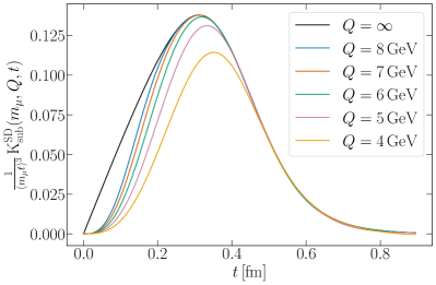
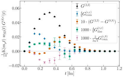
Figure 1: Left: Illustration of the modified short-distance kernels according to eq. (17) with varying virtuality. Right: Integrands for the computation of $(a_{\mu}^{\rm hvp})^{\rm SD}$ on ensemble E250 with near physical quark masses at $a\approx 0.064\,$fm. Smaller contributions have been scaled as indicated in the plot.

To illustrate the behaviour and the relative size of the contributions to $(a_{\mu}^{\rm hvp})^{\rm SD}$, we show in the right panel of Figure 1 integrands of the various contributions according to eq. (14), i.e., without subtraction, where the smaller contributions are scaled as indicated in the figure to show them on the same scale. The ${\scriptstyle\rm L}{\scriptstyle\rm C}$ discretization is displayed for the quark-connected contributions and the ${\scriptstyle\rm C}{\scriptstyle\rm C}$ discretization for the two quark-disconnected contributions. The charm-connected correlation function contributes significantly to the final result for $(a_{\mu}^{\rm hvp})^{\rm SD}$. Except for the two charm-disconnected contributions, the relative statistical uncertainties are very small.

As outlined above, we non-perturbatively compute the subtracted observables $(a_{\mu}^{{d},{e}})^{\rm SD}_{{\rm sub}}(Q^{2})$ according to eq. (17). After the combination with $b^{({d},{e})}(Q^{2})$, eq. (16), the dependence on the virtuality $Q$ has to cancel. We perform our calculation for several values of $Q$ to explicitly test this. For our final result, we choose $Q=5\,$GeV as a good compromise between a high enough scale for the perturbative evaluation of the Adler function and a smoothly varying kernel function ${\rm K}_{\rm sub}^{\rm SD}(m_{\mu},Q,x_{0})$ on the lattice.

If not stated explicitly, all results for the quantities $b^{({d},{e})}$, $(a_{\mu}^{{d},{e}})^{\rm SD}_{{\rm sub}}$ and $(a_{\mu}^{\rm hvp})^{\rm SD}$ are from here on expressed in units of $10^{-10}$.

III.1 Perturbative evaluation of $b(Q^{2})$ in the isovector channel

We have used the perturbative coefficients of the Adler function as given in Baikov:2010je up to $\alpha_{s}^{3}$ and taking the O($\alpha_{s}^{4}$) term from Baikov:2008jh . The effect is to multiply the parton-level prediction by the factor $(1+(\alpha_{s}/\pi)+\sum_{n=2}^{4}(\alpha_{s}/\pi)^{n}\,d_{n})$.

We use the perturbative Adler function in the $N_{f}=3$ massless theory using $\Lambda_{\overline{\rm MS}}=0.338(12)\,$GeV FlavourLatticeAveragingGroupFLAG:2021npn . The QCD beta function was taken into account up to three-loop order included, and we used the corresponding large-$Q^{2}$ asymptotic solution for $\alpha_{s}$ throughout, after having checked that using instead the numerical solution for $\alpha_{s}$ makes an entirely negligible difference. As expected, the convergence of perturbation theory is excellent. For instance, at $Q=5\,$GeV, the set of values of the subtraction term, from the parton-level prediction to the highest-order prediction read

$$b^{({3},{3})}(25\,{\rm GeV}^{2})=\{7.422,~{}7.971,~{}8.037,~{}8.057,~{}8.068\}.$$ (39)

Table 2 lists the perturbative results for several values of $Q^{2}$. Secondly, the uncertainty of $\Lambda_{\overline{\rm MS}}$ induces an absolute uncertainty of $0.011$ on $b^{({3},{3})}(25\,{\rm GeV}^{2})$. Thirdly, the sea-quark effect due to the strange quark is small. In the estimates above, the strange-quark mass is treated as zero. Evaluating the expression in the $N_{f}=2$ massless theory (corresponding to $m_{s}=\infty$) with $\Lambda_{\overline{\rm MS}}=0.330\,$GeV FlavourLatticeAveragingGroupFLAG:2021npn , we obtain

$$b^{({3},{3})}(25\,{\rm GeV}^{2})=8.020\quad\qquad(N_{f}=2).$$ (40)

The comparison of Eqs. (39) and (40) shows that the effect of changing $m_{s}=0$ to $m_{s}\simeq 100$ MeV must be negligibly small, since it is parametrically suppressed by $m_{s}^{2}/Q^{2}$. Finally, we have checked that the phenomenologically estimated gluon and quark ‘condensates’ Eidelman:1998vc make a negligible contribution.

Anticipating that the quantity $b^{({3},{3})}(25\,{\rm GeV}^{2})$ is the only perturbative prediction that enters our final result for $(a_{\mu}^{\rm hvp})^{\rm SD}$, we take as its full uncertainty the linear sum of the error from $\Lambda_{\overline{\rm MS}}$ and the size of the last (O($\alpha_{s}^{4}$)) perturbative term,

$$b^{({3},{3})}(25\,{\rm GeV}^{2})=8.068\pm 0.022.$$ (41)

$Q$[GeV] $b^{({3},{3})}(Q^{2})$ $b^{({\rm c},{\rm c})}(Q^{2})$ 3.5 16.740(43)(34) 20(12) 4.0 12.727(26)(22) 16.3(5.1) 5.0 8.068(11)(11) 11.4(1.3) 6.0 5.567(6)(6) 8.57(45) 7.0 4.072(3)(4) 6.66(17) 8.0 3.106(2)(3) 5.31(8)

Table 2: The perturbatively computed subtraction terms $b^{({3},{3})}(Q^{2})$ and $b^{({\rm c},{\rm c})}(Q^{2})$ (in units of $10^{-10}$) for the isovector and the charm correlator respectively. The former is computed using the $N_{f}=3$ massless perturbative Adler function to O$(\alpha_{s}^{4})$ included, the latter with the massive perturbation theory to O$(\alpha_{s}^{2})$ included, in the expansion with respect to the ratio $(m_{c}^{2}/Q^{2})$ to third order included. The first number in brackets indicates the absolute size of the last O($\alpha_{s}^{n}$) term included in the estimate and gives an indication of the uncertainty related to the convergence of the perturbative series. For $b^{({3},{3})}$, the uncertainty induced by that on $\Lambda_{\overline{\rm MS}}$ is indicated as well.

III.2 Non-perturbative evaluation of $(a_{\mu}^{\rm hvp})^{\rm SD}_{\rm sub}(Q^{2})$ in the isovector channel

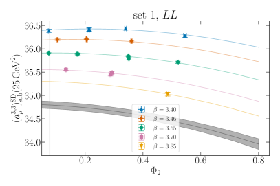
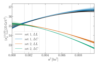
Figure 2: Illustration of fits to $(a_{\mu}^{{3},{3}})^{\rm SD}_{{\rm sub}}(25\,{\rm GeV}^{2})$. Left: Best fit, according to its model weight, to the data for set 1, ${\scriptstyle\rm L}{\scriptstyle\rm L}$. The data is corrected for deviation from physical $\Phi_{4}$. The coloured lines show the evaluation of the fit function at finite lattice spacing. The black line, together with the grey band, show the dependence on $\Phi_{2}$ in the continuum limit. Right: Approaches to the continuum limit for four sets of data based on the improvement schemes of set 1 and 2 and the ${\scriptstyle\rm L}{\scriptstyle\rm L}$ and ${\scriptstyle\rm L}{\scriptstyle\rm C}$ discretizations of the current based on a scan over fit models for $(a_{\mu}^{{3},{3}})^{\rm SD}_{{\rm sub}}(25\,{\rm GeV}^{2})$. Each line shows the result from one single fit and the opacity of the lines corresponds to the weight of the fit in the model average. Dashed vertical lines indicate the lattice spacings used in this work.

In the short-distance regime, no signal-to noise problem hinders the computation in the isovector channel and the precise lattice data can be integrated by summation. We evaluate $(a_{\mu}^{\rm hvp})^{\rm SD}_{\rm sub}$ at several values of $Q^{2}$ to be able to monitor the convergence of the sum in eq. (15) and to investigate whether the choice of $Q^{2}$ has an influence on the systematic uncertainties of the lattice evaluation.

The small finite-volume effects are corrected using the method by Hansen and Patella Hansen:2019rbh ; Hansen:2020whp , see Ce:2022kxy for the details of our implementation. We find the size of the correction to be at most two permille on the ensembles included in our computation. Finite-volume corrections due to kaon loops are non-negligible close to the SU(3) symmetric point, where pion and kaon masses are of similar order. We use the same procedure as for the effects from pions to estimate the corresponding correction. Both contributions and their sum are given in table 5. A flat $25\%$ systematic uncertainty is assigned to the corrections.

As explained above, we scan a variety of ansätze for the chiral-continuum extrapolation to determine $(a_{\mu}^{{3},{3}})^{\rm SD}_{{\rm sub}}$ at the physical point. The best fit according to the AIC for the data of set 1 with the ${\scriptstyle\rm L}{\scriptstyle\rm L}$ discretization is shown on the left-hand side of Figure 2. The minimized $\chi^{2}$ is $7.64$ for 11 degrees of freedom (dof). We show the dependence of $(a_{\mu}^{{3},{3}})^{\rm SD}_{{\rm sub}}(25\,{\rm GeV}^{2})$ on the light quark mass proxy $\Phi_{2}$, where the data has been corrected for deviations from $\Phi_{4}^{\rm phys}$ and cuts to $m_{\pi}<400\,{\rm MeV}$ and $a<0.09\,$fm have been applied. The data and the fit function are shown for the five values of the inverse gauge coupling that are included in this fit. As visible from the figure, the quark mass effects are mild but depend on the lattice spacing. The fit also includes cutoff effects proportional to $a^{2}\Phi_{4}$ which are not visible in the plot.

On the right-hand side of Figure 2, we show the approach to the continuum limit at physical quark masses, as determined from the scan over all fit models for both discretizations of the current and both improvement schemes. Each line corresponds to one fit and the opacity is related to the model weight of the fit according to the AIC. The relative size of the cutoff effects, about $10\%$ in the most extreme case, is not larger than in our computation of the intermediate-distance window observable Ce:2022kxy , thanks to some of the improvements described in section II.3. For the same reason, the difference between the two discretizations of the current is small.

The two sets of improvement schemes lead to cutoff effects that have opposite signs. A similar behaviour has been observed for the case of the intermediate-distance window, where the extrapolations of both data sets agreed in the continuum limit, taking into account the curvature in the extrapolation of the set 2 data. In the case of $(a_{\mu}^{{3},{3}})^{\rm SD}_{{\rm sub}}$ we observe that most of the fits from set 2 with a large model weight favour slightly larger values than the fits to the data of set 1. However, for some fits we observe a strong curvature at very small values of the lattice spacing such that they are compatible with the more benign extrapolations for set 1. In the current situation, where we do not have more information on the behaviour towards the continuum limit, e.g., by adding data at even finer lattice spacings, we decide to take the discrepancy between the two data sets into account as systematic uncertainty of our continuum extrapolation.

We perform the model average over the four data sets, using a flat relative weight between the sets and arrive at

$$(a_{\mu}^{{3},{3}})^{\rm SD}_{{\rm sub}}(25\,{\rm GeV}^{2})=35.03(4)_{\rm stat}(21)_{\rm syst}(3)_{\rm scale}[22]\,.$$ (42)

Whereas the systematic uncertainty of $0.21$ amounts to about $0.6\%$ of the value of $(a_{\mu}^{{3},{3}})^{\rm SD}_{{\rm sub}}$, we note that it is sub-permille with respect to $a_{\mu}^{{3},{3}}$. The description of the short-distance cutoff effects therefore does not seem to be a roadblock towards the target precision for the full HVP.

The qualitative behaviour of the continuum extrapolation does not vary with the choice of $Q^{2}$. A smaller value of $Q^{2}$, which removes more of the potentially difficult ultra short-distance region, does not lead to a better agreement of the results based on the two improvement schemes.

III.3 Combination of perturbative and non-perturbative evaluations in the isovector channel

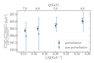
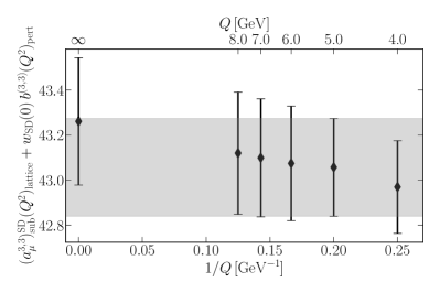
Figure 3: Left: The ratio $(b^{({3},{3})}(Q^{2})-b^{({3},{3})}(Q_{\rm ref}^{2}))/(1/Q^{2}-1/Q_{\rm ref}^{2})$ with $Q_{\rm ref}^{2}=(8\,{\rm GeV})^{2}$ for the isovector channel, computed non-perturbatively in lattice QCD vs. using the perturbative Adler function (see eqs. (9), (16) and (19)). For visibility, the data is slightly displaced horizontally. Right: Stability of the result for $(a_{\mu}^{{3},{3}})^{\rm SD}$ as a function of the virtuality $Q^{2}$ chosen in the perturbatively treated subtraction term. Choosing $Q=\infty$ corresponds to the entire $(a_{\mu}^{{3},{3}})^{\rm SD}$ being computed in lattice QCD without any use of perturbation theory.

The non-perturbative evaluation of $(a_{\mu}^{\rm hvp})^{\rm SD}_{\rm sub}$ at several values of $Q^{2}$ gives us the possibility to monitor the convergence of perturbation theory and to directly compare the perturbative and non-perturbative evaluations of the difference in eq. (19). We choose the reference energy $Q_{\rm ref}=8\,$GeV where the convergence of perturbation theory is expected to be excellent.

In the non-perturbative evaluation, we compute the left hand side of eq. (19). We get compatible results when performing the difference either in the continuum limit or when subtracting ensemble by ensemble and extrapolating the difference. We choose the second version for the comparison with perturbation theory in Figure  3. It can be seen that both approaches give essentially the same results down to $Q=4\,$GeV, confirming the good convergence of the perturbative series.

On the right-hand side of Figure 3 we depict the final quantity $(a_{\mu}^{{3},{3}})^{\rm SD}$ depending on the choice of $Q$. Any dependence on $Q$ should be removed after combining lattice and perturbation theory and indeed all results are entirely compatible with each other. For our final estimate, we use $Q=5\,$GeV and obtain

$$(a_{\mu}^{{3},{3}})^{\rm SD}=43.06(4)_{\rm stat}(21)_{\rm syst}(3)_{\rm scale}[22]\,.$$ (43)

We also show a result for the direct evaluation of $(a_{\mu}^{{3},{3}})^{\rm SD}$, without any subtraction in the kernel function, in Figure 3, where we have ignored the possibility of cutoff effects of $\mathrm{O}(a^{2}\log(a))$ Ce:2021xgd being present in the lattice data and employed the same set of continuum extrapolations as for the subtracted quantity. The agreement with our final result is an indication that the size of these effects is small for this specific observable.

III.4 Non-perturbative evaluation of $\Delta_{\rm ls}(a_{\mu})^{\rm SD}$

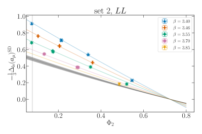
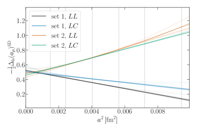
Figure 4: Illustration of fits to $\Delta_{\rm ls}(a_{\mu})^{\rm SD}$. Left: Best fit, according to its model weight, to the data for set 2, ${\scriptstyle\rm L}{\scriptstyle\rm L}$ with $\chi^{2}/{\rm dof}=13.07/13$. The data is corrected for deviation from physical $\Phi_{4}$. The coloured lines show the evaluation of the fit function at finite lattice spacing. The black line, together with the gray band, show the dependence on $\Phi_{2}$ in the continuum limit. Right: Projection onto the lattice spacing dependence and physical quark masses for the best fits in the four categories entering the model average.

To compute the isoscalar contribution to $(a_{\mu}^{\rm hvp})^{\rm SD}$, it suffices to evaluate $\Delta_{\rm ls}(a_{\mu})^{\rm SD}$ as given by eq. (21). The quark-disconnected loops for light and strange quarks, computed as outlined in Ce:2022eix , enter here and may be precisely determined in the short-distance region. By definition, the splitting $\Delta_{\rm ls}(a_{\mu})^{\rm SD}$ vanishes at the SU(3) symmetric point and is expected to depend at leading order on $m_{\rm s}-m_{\rm l}$. We take this knowledge into account for the chiral and continuum extrapolation. Defining $\Phi_{\delta}=\Phi_{4}-\frac{3}{2}\Phi_{2}$, we parametrize

$$\Delta_{\rm ls}(a_{\mu})^{\rm SD}(\Phi_{\delta},\Phi_{4},X_{a})=\Phi_{\delta}\left(\gamma_{1}+\gamma_{2}\Phi_{\delta}+\beta_{2}X_{a}^{2}+\beta_{3}X_{a}^{3}+\gamma_{0}\Phi_{4}\right)\,,$$ (44)

and again build a variety of ansätze by setting coefficients to zero. The ensembles with SU(3) symmetry are excluded from these fits. All cutoff effects are suppressed by $\Phi_{\delta}$ close to the SU(3) symmetric point.

On the left-hand side of figure 4 we show the $\Phi_{2}$ dependence for the data and a typical fit for set 2 and the ${\scriptstyle\rm L}{\scriptstyle\rm L}$ discretization. The constraint $\Delta_{\rm ls}(a_{\mu})^{\rm SD}=0$ for $\Phi_{4}=\frac{3}{2}\Phi_{2}$ at the SU(3) symmetric point is visible by the intersection of the curves which denote the $\Phi_{2}$ dependence at finite lattice spacing and in the continuum, respectively. Towards the physical point, cutoff effects grow since the suppression is lifted. On the right-hand side of the figure, we show the approach to the continuum for all fits that are contained in the scan over the different models, evaluated at physical light and strange quark masses. The data from set 1 approach the continuum value from below whereas the cutoff effects for data set 2 have the opposite sign.

With the result

$${\textstyle\frac{1}{3}}\Delta_{\rm ls}(a_{\mu})^{\rm SD}=-0.495(7)_{\rm stat}(34)_{\rm syst}(4)_{\rm scale}[36]\,,$$ (45)

from an average over the fit models, eq. (21) and the result for the isovector contribution from eq. (43), we arrive at

$${\textstyle\frac{1}{3}}(a_{\mu}^{{8},{8}})^{\rm SD}=13.857(14)_{\rm stat}(78)_{\rm syst}(7)_{\rm scale}[81]\,,$$ (46)

for the isoscalar contribution. We note that this result has significant correlation with the result for $(a_{\mu}^{{3},{3}})^{\rm SD}$, which is taken into account when combining both in $(a_{\mu}^{\rm hvp})^{\rm SD}$.

For comparison with other lattice results, we combine the results for the isovector and isoscalar contributions in eqs. (43) and (46) to compute the strange-connected contribution,

$${\textstyle\frac{1}{9}}(a_{\mu}^{{\rm s},{\rm s}})^{\rm SD}=9.072(10)_{\rm stat}(58)_{\rm syst}(3)_{\rm scale}[60]\,.$$ (47)

The disconnected contribution from light and strange quark loops is found to be irrelevant with respect to the precision quoted here. A direct evaluation of the strange-connected contribution via the same strategy as for the charm-connected contribution gives a result that is fully compatible with eq. (47).

III.5 Evaluation of the charm-connected contribution

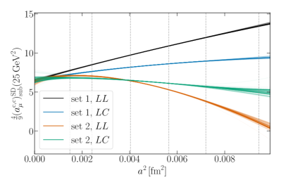
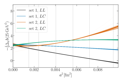
Figure 5: Lattice spacing dependence from a scan over fit models for four data sets. The lattice spacings used in this work are indicated by vertical lines. Left: fits to $(a_{\mu}^{{\rm c},{\rm c}})^{\rm SD}_{{\rm sub}}(36\,{\rm GeV}^{2})$. Right: fits to $-{\textstyle\frac{4}{9}}\Delta_{\rm lc}b(25\,{\rm GeV}^{2})$.

To compute the charm-connected contribution on the lattice, we start by evaluating $(a_{\mu}^{{\rm c},{\rm c}})^{\rm SD}_{{\rm sub}}(Q^{2})$. The tuning of the charm quark hopping parameter to match the mass of the $D_{\rm s}$ meson of 1968.47 MeV and the determination of the renormalization constant for the local charm current in a massive renormalization scheme have been described in Gerardin:2019rua ; Ce:2022kxy . After the continuum extrapolation, we perform a small correction to adapt the tuning to the updated value of the scale setting quantity $t_{0}^{\rm phys}$ from Strassberger:2021tsu .

In contrast to the isovector contribution, we find very good agreement of the continuum extrapolations of the four data sets, despite having significantly different cutoff effects. We illustrate the cutoff effects based on the scan over the fit models for each of the four data sets on the left-hand side of Figure 5. For our final value, in line with our previous work, we use only the ${\scriptstyle\rm L}{\scriptstyle\rm C}$ discretization of the current, since it exhibits significantly smaller cutoff effects.

The effect of massive quarks in the contribution $b^{({\rm c},{\rm c})}$ may be computed on the lattice without potentially dangerous log-enhanced cutoff effects. The size of this contribution strongly depends on the choice of $Q$ and at large values of $Q$, the observable is dominated by distances $<0.3\,$fm. On the right-hand side of Figure 5 we show the approaches to the continuum, based on the scan of the fit models. We evaluate $\Delta_{\rm lc}b(Q^{2})$ for the same values of $Q^{2}$ as $(a_{\mu}^{{3},{3}})^{\rm SD}$ to explore the parameter space and to be able to compare to the evaluation of the same observable using massive perturbation theory, see table 2.

The perturbative evaluation is based on the expansion in $\overline{m}_{c}^{2}/Q^{2}$ of the vacuum polarization, computed to O($\alpha_{s}^{2}$) in Chetyrkin:1997qi . We have kept expansion terms up to O($(\overline{m}_{c}^{2}/Q^{2})^{4}$) in the perturbative orders $\alpha_{s}^{0}$ and $\alpha_{s}$, while we kept expansion terms up to O($(\overline{m}_{c}^{2}/Q^{2})^{3}$) in the O($\alpha_{s}^{2}$) contribution. When computing $b^{({\rm c},{\rm c})}(Q^{2})$, we evaluate $\alpha_{s}$ as well as the $\overline{\rm MS}$ charm mass at a scale $\mu^{2}$ given by the geometric mean of $Q^{2}$ and $Q^{2}/4$, using the FLAG’21 FlavourLatticeAveragingGroupFLAG:2021npn value of $\Lambda_{\overline{\rm MS}}$ and starting from the PDG value $\overline{m}_{c}(\mu=\overline{m}_{c})=1.27\,$GeV ParticleDataGroup:2020ssz . The number indicated in brackets in the $b^{({\rm c},{\rm c})}$ column of table 2 represents the contribution of the O($\alpha_{s}^{2}$) term as a way to indicate the uncertainty of the prediction. The quark-mass dependent contribution to $b^{({\rm c},{\rm c})}(Q^{2})$ is compared to lattice data in Fig. 6.

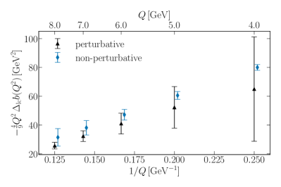
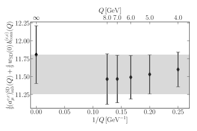
Figure 6: Left: The difference ${-\textstyle\frac{4}{9}}Q^{2}\,\Delta_{\rm lc}b(Q^{2})$ computed non-perturbatively in lattice QCD vs. using massive perturbation theory. For visibility, the data is slightly displaced horizontally. Right: Stability of the result for $(a_{\mu}^{{\rm c},{\rm c}})^{\rm SD}$ as a function of the virtuality $Q^{2}$ chosen in the subtraction term. Choosing $Q=\infty$ corresponds to the entire $(a_{\mu}^{{\rm c},{\rm c}})^{\rm SD}$ being computed in lattice QCD without any use of perturbation theory.

On the left-hand side of Figure 6, we show the comparison of the perturbative prediction and the lattice result for $\Delta_{\rm lc}b(Q^{2})$ in the form proposed in eq. (19). We choose $Q_{\rm ref}=\infty$ where $\Delta_{\rm lc}$ has to vanish. It is visible that at small $Q$, despite giving similar central values, the uncertainty on the perturbative result is significantly larger than the uncertainty on the lattice evaluation, which is dominated by the systematic uncertainty from the continuum extrapolation. We note that the relative size of this uncertainty grows with increasing $Q$, whereas its absolute size decreases.

For our final result, we combine the non-perturbative evaluations of $(a_{\mu}^{{\rm c},{\rm c}})^{\rm SD}_{{\rm sub}}(Q^{2})$ and $\Delta_{\rm lc}b(Q^{2})$ with the perturbative result for $b^{({3},{3})}(Q^{2})$. The combination for several values of $Q^{2}$ is shown on the right-hand side of Figure 6. The residual dependence on $Q$ is negligible with respect to the uncertainties. For our final result, we again choose $Q=5\,$GeV and with

$${\textstyle\frac{4}{9}}(a_{\mu}^{{\rm c},{\rm c}})^{\rm SD}_{{\rm sub}}(25\,{\rm GeV}^{2}) {}=\phantom{-}6.81(9)_{\rm stat}(21)_{\rm syst}(7)_{\rm scale}[25]\,,$$ (48)

$${\textstyle\frac{4}{9}}\Delta_{\rm lc}b(25\,{\rm GeV}^{2}) {}=-2.42(4)_{\rm stat}(10)_{\rm syst}(3)_{\rm scale}[11]\,,$$ (49)

we arrive at

$${\textstyle\frac{4}{9}}(a_{\mu}^{{\rm c},{\rm c}})^{\rm SD}=11.53(13)_{\rm stat}(23)_{\rm syst}(11)_{\rm scale}[30]\,.$$ (50)

III.6 The charm-disconnected contributions

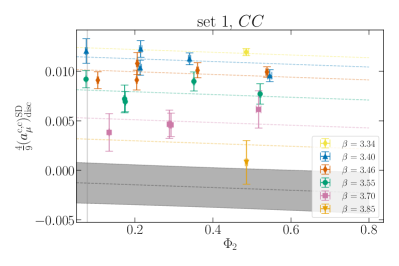
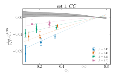
Figure 7: Illustration of typical fits to the charm-disconnected contributions. The data is corrected for deviations from $\Phi_{4}^{\rm phys}$. The coloured lines show evaluations of the fit function at finite lattice spacing and the grey area show the result in the continuum limit. Left: Fit to ${\textstyle\frac{4}{9}}(a_{\mu}^{{\rm c},{\rm c}})^{\rm SD}_{\rm disc}$ with $\chi^{2}/{\rm dof}=17.60/16$. Right: Fit to ${\textstyle\frac{2}{3\sqrt{3}}}(a_{\mu}^{{\rm c},{\rm 8}})^{\rm SD}_{\rm disc}$ with $\chi^{2}/{\rm dof}=9.20/12$.

The quark-disconnected contributions including charm quarks have not been included in our previous results for $a_{\mu}^{\rm hvp}$ Gerardin:2019rua and $(a_{\mu}^{\rm hvp})^{\rm ID}$ Ce:2022kxy because they are expected to be numerically very small and mostly contained in the short-distance region. In this work, we compute the contributions $G^{({\rm c},{8})}$ and $G^{({\rm c},{\rm c})}_{\rm disc}$ in a partially quenched setup, see Appendix C of Ce:2022eix for an explanation of the computational setup. The charm quark hopping parameter is set to the same value as in the quark-connected case. To avoid mixing with the singlet current at $\mathrm{O}(a)$ in the case of $G^{({\rm c},{8})}$, and anticipating smaller cutoff effects in the case of a heavy quark (see section III.5), we evaluate the correlation functions with conserved vector currents at source and sink.

We find both contributions to be very small and, at finite lattice spacing, non-zero only below a distance of about 1 fm. Given the smallness of these contributions, we perform the analysis without subtractions in the kernel function, ignoring the possibility of log-enhanced cutoff effects.

The charm-charm contribution is dominated by cutoff effects, already visible by comparing different discretizations of the current on a single ensemble. We find significantly different integrands and even a change in sign when employing the ${\scriptstyle\rm L}{\scriptstyle\rm L}$ formulation of the current instead of ${\scriptstyle\rm C}{\scriptstyle\rm C}$ or ${\scriptstyle\rm L}{\scriptstyle\rm C}$. Accordingly, the relative size of the cutoff effects is found to be large in the continuum extrapolation. On the left-hand side of Figure 7 we show an exemplary chiral-continuum extrapolation for this contribution. As can bee seen in the figure, the sign changes from positive to negative when taking the continuum limit. We attribute the slight light quark mass dependence to the matching of the charm quark via the mass of the $D_{\rm s}$ meson and the variation of the strange quark mass in our set of ensembles. At the physical point we find after averaging over the fit models the value

$${\textstyle\frac{4}{9}}(a_{\mu}^{{\rm c},{\rm c}})^{\rm SD}_{\rm disc}=-0.0010(18)_{\rm stat}(32)_{\rm syst}(1)_{\rm scale}[37]\,,$$ (51)

and thus only an upper limit on the magnitude of this contribution.

Since the contribution $(a_{\mu}^{{c},{8}})^{\rm SD}$ is SU(3) suppressed, we employ fits according to eq. (44). An example fit is shown on the right-hand side of Figure 7. Cutoff effects are suppressed close to the SU(3) symmetric point but significant at physical quark mass. The chiral-continuum extrapolated value is compatible with zero. We obtain

$${\textstyle\frac{2}{3\sqrt{3}}}(a_{\mu}^{{\rm c},{\rm 8}})^{\rm SD}_{\rm disc}=0.0020(17)_{\rm stat}(25)_{\rm syst}(0)_{\rm scale}[31]\,,$$ (52)

from averaging over all fit models.

Both contributions are thus negligible compared to $(a_{\mu}^{\rm hvp})^{\rm SD}$ (and our final uncertainty). Naturally, this carries over to $a_{\mu}^{\rm hvp}$. Summing the two results above and adding the disconnected contribution that enters our final result via $(a_{\mu}^{{8},{8}})^{\rm SD}$, we quote

$$(a_{\mu}^{\rm hvp})^{\rm SD}_{\rm disc}=0.0013(25)_{\rm stat}(41)_{\rm syst}(5)_{\rm scale}[49]$$ (53)

to allow for a comparison with other works.

III.7 Isospin-breaking corrections

We apply two complementary methods to determine isospin-breaking effects in $(a_{\mu}^{\rm hvp})^{\rm SD}$. The first employs massless QCD perturbation theory to compute the leading QED effects. The second approach is based on the explicit calculation of isospin-breaking corrections due to unequal up and down quark masses and electric charges, following the same method as in our previous publication on the intermediate-distance window observable Ce:2022kxy .

To compute the leading QED effects at short distances in massless QCD perturbation theory, we start from the expression for the relative correction to the Adler function (see Kataev:1992dg , where the correction is given for the $R$ ratio)

$$\frac{D_{\rm QCD,1\,internal\,\gamma}(Q^{2})}{D_{\rm QCD}(Q^{2})}=\frac{\alpha}{\pi}\cdot\left(\frac{3}{4}-\frac{\alpha_{s}}{\pi}+{\rm O}(\alpha_{s}^{2})\right)\frac{\sum_{f=u,d,s}{\cal Q}_{f}^{4}}{\sum_{f=u,d,s}{\cal Q}_{f}^{2}}\,.$$ (54)

Note that in this notation $D_{\rm QCD}(Q^{2})=3(1+(\alpha_{s}/\pi)+{\rm O}(\alpha_{s}^{2}))\sum_{f=u,d,s}{\cal Q}_{f}^{2}$ is the pure massless QCD expression, while $D_{\rm QCD,1\,internal\,\gamma}(Q^{2})$ is the contribution from massless QCD containing exactly one internal photon line. The ratio (54) amounts to $0.51\times 10^{-3}$ for $\alpha_{s}=0.30$ for the $(u,d,s)$ contribution, and to $0.57\times 10^{-3}$ if one restricts one’s attention to the $(u,d)$ sector. These are very small corrections indeed, yielding the estimate $[(a_{\mu}^{{3},{3}})^{\rm SD}+{\textstyle\frac{1}{3}}(a_{\mu}^{{8},{8}})^{\rm SD}]_{\rm 1\,internal\,\gamma}=0.03$. For the QED correction to the charm contribution, we use the KS spectral function expressed in terms of the $\overline{\rm MS}$ charm mass. This means that the latter mass is kept fixed as the electromagnetic interaction is ‘turned on’. The free-quark level contribution of the charm is $\frac{4}{9}(a_{\mu}^{{\rm c},{\rm c}})^{\rm SD}=11.6$ using the mass of $\overline{m}_{c}(\overline{m}_{c})=1.27\,$GeV, while the relative QED correction to that is $0.83\times 10^{-3}$. In absolute terms, this means

$${\textstyle\frac{4}{9}}(a_{\mu}^{{\rm c},{\rm c}})^{\rm SD}({\rm 1\,internal\,\gamma})=0.01.$$ (55)

For our second approach we have computed $(a_{\mu}^{\rm hvp})^{\rm SD}$ in QCD+QED on a subset of our ensembles using Monte Carlo reweighting combined with the leading-order perturbative expansion of QCD+QED about the isosymmetric theory deDivitiis:2013xla ; Risch:2021hty ; Risch:2019xio ; Risch:2018ozp ; Risch:2017xxe . The same method was applied in Ref. Ce:2022kxy . In order to determine the dependence of isospin-breaking corrections to the short-distance window observable on the pion mass and the lattice spacing, we have used eight ensembles (A654, H102, N101, N452, N451, D450, N203 and N200), covering a much wider range of pion masses ($220-350$ MeV) and lattice spacings ($0.064-0.097$ fm) compared to our previous calculation Ce:2022kxy . As before, we define our hadronic renormalization scheme in terms of $m_{\pi^{0}}^{2}$, $m_{K^{+}}^{2}+m_{K^{0}}^{2}-m_{\pi^{+}}^{2}$, $m_{K^{+}}^{2}-m_{K^{0}}^{2}-m_{\pi^{+}}^{2}+m_{\pi^{0}}^{2}$ and the fine-structure constant $\alpha$. Neglecting isospin-breaking effects in the lattice scale and in the quark sea, as well as quark-disconnected contributions in the calculation of the relevant correlation functions, we realize our scheme by matching the values of $m_{\pi^{0}}^{2}$ and $m_{K^{+}}^{2}+m_{K^{0}}^{2}-m_{\pi^{+}}^{2}$ in QCD+QED to those in the isosymmetric theory and by setting $m_{K^{+}}^{2}-m_{K^{0}}^{2}-m_{\pi^{+}}^{2}+m_{\pi^{0}}^{2}$ to its experimental value. Further technical details are described in section VI of Ref. Ce:2022kxy .

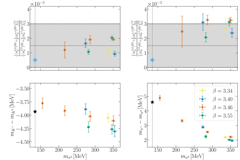
Figure 8: The relative strong and electromagnetic isospin-breaking corrections to the connected light and strange quark contribution computed using the conserved-local (upper left panel) and local-local (upper right panel) discretizations of the vector current. The light blue crosses denote the prediction from massless QCD (see the main text). The dashed line and the grey area show our final estimate. The two panels at the bottom show the mass splittings of charged and neutral kaons and pions, respectively. The black stars represent the experimental values.

Our results for the relative size of the isospin-breaking corrections to the connected light and strange contributions to $(a_{\mu}^{\rm hvp})^{\rm SD}$ are shown in the upper panel of Figure 8 for the conserved-local (left) and local-local (right) combinations of vector currents. We make two observations: first, the relative corrections are very small and typically amount to a few per-mil. Second, there is no clear dependence of the results on the pion mass and the lattice spacing, which would allow for a systematic extrapolation to the physical point. On the other hand, our results for the meson mass splittings $m_{K^{+}}-m_{K^{0}}$ and $m_{\pi^{+}}-m_{\pi^{0}}$, shown in the lower panels of Figure 8, and which include an additional ensemble at almost physical pion mass (D452), show a consistent trend towards the corresponding experimental values. We are, therefore, confident that the typical size of isospin-breaking corrections to $(a_{\mu}^{\rm hvp})^{\rm SD}$ has been determined correctly. Taking into account the spread in the results and allowing for a generous error, we represent the data shown in the upper panels of Figure 8 by $(1.5\pm 1.5)\times 10^{-3}$. We can then work out the absolute correction to the connected light and strange quark contribution, by multiplying the sum of eqs. (43) and (47) with 0.0015, which yields

$$[(a_{\mu}^{{3},{3}})^{\rm SD}+{\textstyle\frac{1}{9}}(a_{\mu}^{{\rm s},{\rm s}})^{\rm SD}]\times 0.0015=0.085\,.$$ (56)

Adding the QED correction to the charm quark contribution of 0.01 from eq. (55) and assuming an uncertainty of 100% for the latter, we arrive at

$$[(a_{\mu}^{{3},{3}})^{\rm SD}+{\textstyle\frac{1}{9}}(a_{\mu}^{{\rm s},{\rm s}})^{\rm SD}+{\textstyle\frac{4}{9}}(a_{\mu}^{{\rm c},{\rm c}})^{\rm SD}]_{\rm SIB,\,QED}=0.095(95)\,,$$ (57)

which we quote as the total isospin-breaking correction to $(a_{\mu}^{\rm hvp})^{\rm SD}$. This number is larger but of the same order of magnitude compared to the QED correction to $[(a_{\mu}^{{3},{3}})^{\rm SD}+{\textstyle\frac{1}{3}}(a_{\mu}^{{8},{8}})^{\rm SD}+{\textstyle\frac{4}{9}}(a_{\mu}^{{\rm c},{\rm c}})^{\rm SD}]$ estimated in massless QCD perturbation theory at leading order and denoted by the light blue crosses in Fig. 8, which further corroborates our findings.

III.8 Further, small contributions

In this section, we present our (mostly perturbative) estimates for two small contributions that we did not evaluate directly in lattice QCD.

For the contribution of the $b$ quark, $(a_{\mu}^{{\rm b},{\rm b}})^{\rm SD}$, the perturbative spectral function is known exactly to O($\alpha_{s}$) from the calculation of Källén-Sabry (KS) Kallen:1955fb , described for instance in Chetyrkin:1996ela . The O($\alpha_{s}^{2}$) corrections were calculated in Chetyrkin:1995ii . We have evaluated the KS prediction, improved by substituting the pole quark-mass appearing in $R(s)$ by its $\overline{\rm MS}$ counterpart and evaluating the latter at the scale $s$. Using the PDG bottom mass of 4.18 GeV, this results in the estimate ${\textstyle\frac{1}{9}}(a_{\mu}^{{\rm b},{\rm b}})^{\rm SD}=0.31$.

We also note the NRQCD based lattice calculation Colquhoun:2014ica , which finds ${\textstyle\frac{1}{9}}a_{\mu}^{\rm b,b}=0.271(37)$, while the phenomenological estimate Erler:2021bnl based on sum rules obtains $0.30(2)$. We have checked that the bottom contribution to ${\textstyle\frac{1}{9}}(a_{\mu}^{\rm b,b}-(a_{\mu}^{{\rm b},{\rm b}})^{\rm SD})$ is on the order of $0.003$. We thus arrive at our estimate of

$${\textstyle\frac{1}{9}}(a_{\mu}^{{\rm b},{\rm b}})^{\rm SD}=0.29(3).$$ (58)

As for the effect of the missing charm sea quarks in our lattice calculation, we estimate its order of magnitude based on perturbation theory, rather than on $D$ meson loops as we previously did for the intermediate window in Ce:2022kxy , since $(a_{\mu}^{\rm hvp})^{\rm SD}$ involves relatively short distances. Using the perturbative results of Hoang:1994it , we estimate the effect to be at the level of

$$[(a_{\mu}^{{3},{3}})^{\rm SD}+{\textstyle\frac{1}{3}}(a_{\mu}^{{8},{8}})^{\rm SD}]_{\rm pert.\,charm\,sea\,quark\,effect}=0.02.$$ (59)

Note that the perturbative estimate of the connected charm contribution is in rather good agreement with the lattice calculation (see the text above eq. (55)). Nevertheless, since eq. (59) represents only the leading perturbative prediction for the effect under scrutiny, we will conservatively assign an uncertainty of

$$\Delta[(a_{\mu}^{{3},{3}})^{\rm SD}+{\textstyle\frac{1}{3}}(a_{\mu}^{{8},{8}})^{\rm SD}]_{\rm charm\,quenching}=0.10$$ (60)

to our calculation due to the quenching of the charm quark.

IV Conclusion

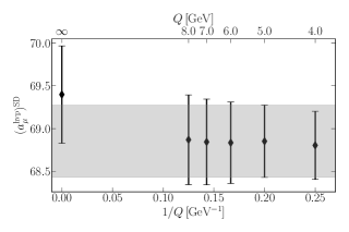
Figure 9: Left: Residual $Q$ dependence of $(a_{\mu}^{\rm hvp})^{\rm SD}$. The grey area shows the final result. Right: Contributions to the variance of $(a_{\mu}^{\rm hvp})^{\rm SD}$ as evaluated for $Q=5\,$GeV.

Combining the results of sections III, we arrive at the result

$$(a_{\mu}^{\rm hvp})^{\rm SD}=68.85(14)_{\rm stat}(39)_{\rm syst}(15)_{\rm scale}[45]\,,$$ (61)

where all contributions and sources of uncertainty have been taken into account. As outlined in the main text, we have evaluated the subtracted quantity of eq. (17) for $Q^{2}=25\,{\rm GeV}^{2}$. For this choice, 26% of the result in eq. (61) are due to massless perturbation theory applied in the spacelike domain. On the left-hand side of Figure 9 we show results for $(a_{\mu}^{\rm hvp})^{\rm SD}$ for several choices of the virtuality, the grey band denoting our final estimate. No residual dependence on the choice for $Q$ can be resolved. At $Q=4\,$GeV 41% of the result would stem from massless perturbation theory, as given by Table 2, whereas the contribution at $Q=8\,$GeV would only be 10%. We find a noticeable, but not significant difference of our results using $(a_{\mu}^{\rm hvp})^{\rm SD}_{\rm sub}$ with respect to a direct evaluation of $(a_{\mu}^{\rm hvp})^{\rm SD}$, as indicated by the leftmost data point in the figure.

We have shown that, in our data set, $(a_{\mu}^{\rm hvp})^{\rm SD}$ depends much more strongly on the lattice spacing than on the quark masses (see Fig. 2). The very fine lattices employed here were thus instrumental in controlling the continuum limit, even though most of them correspond to heavier-than-physical pion masses. The final uncertainty is dominated by systematic uncertainties, mostly from the variation of models selected to perform the continuum extrapolation. On the right-hand side of Fig. 9, we show the contributions to the squared uncertainty. The contribution labelled ‘statistics’ corresponds to the statistical uncertainty of $0.14$ in eq. (61). The dependence on the scale setting quantity, and therefore also the resulting contribution to the final uncertainty, is dominated by the charm quark contribution and contains the matching with the mass of the $D_{\rm s}$ meson.

In table 3 we collect the dependence of specific (intermediate) results with respect to the quantities that define our scheme of isospin symmetric QCD. The information can be used to adapt the results to a different scheme, provided that the differences in the input quantities are small. For example, a shift in the scale setting quantity $\sqrt{t_{0}^{\rm phys}}$ to the current $N_{\rm f}=2+1+1$ FLAG average with the central value $\sqrt{(t_{0})_{N_{\rm f}=2+1+1}^{\rm phys}}=0.14292\,$fm would result in the adapted value $(a_{\mu}^{\rm hvp})^{\rm SD}=69.00(45)$.

	$S$
$O$	$\sqrt{t_{0}}$	$m_{\pi}$	$m_{K}$	$m_{D_{\rm s}}$
$(a_{\mu}^{{3},{3}})^{\rm SD}$	$-3.47$	$-0.11$	$-0.60$	–
${\textstyle\frac{1}{3}}(a_{\mu}^{{8},{8}})^{\rm SD}$	$-0.70$	$+0.04$	$-1.55$	–
${\textstyle\frac{4}{9}}(a_{\mu}^{{c},{c}})^{\rm SD}$	$-11.37$	$-0.07$	$+3.57$	$-31.05$
$(a_{\mu}^{\rm hvp})^{\rm SD}$	$-15.53$	$-0.14$	$+1.43$	$-31.05$

Table 3: Dimensionless scheme dependencies of observable $O$ with respect to the quantity $S$ according to $S\frac{\partial O}{\partial S}$. The four quantities $S$ define the scheme of isoQCD in this work. Their central values are $\sqrt{t_{0}}=0.1443\,$fm, $m_{\pi}=134.9768\,$MeV, $m_{K}=495.011\,$MeV, $m_{D_{\rm s}}=1968.47\,$MeV.

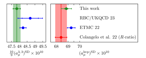
Figure 10: Comparison of our results for the short-distance window observable $(a_{\mu}^{\rm hvp})^{\rm SD}$ (right panel) and the light-quark connected contribution (left panel) to other recent lattice calculations by ETM ExtendedTwistedMass:2022jpw and RBC/UKQCD RBC:2023pvn . Our results are denoted by green circles and band, while the data-driven estimate of Colangelo et al. Colangelo:2022vok is shown as the red circle and band.

A compilation of recent results for the short-distance window observable Colangelo:2022vok ; ExtendedTwistedMass:2022jpw ; RBC:2023pvn , including the estimates from this work, is shown in Figure 10. Our result (61) is in good agreement with the dispersive estimate from Colangelo:2022vok , $(a_{\mu}^{\rm hvp})^{\rm SD}=68.4(5)$. Our result is also in good agreement with the lattice result from the ETM collaboration ExtendedTwistedMass:2022jpw , $(a_{\mu}^{\rm hvp})^{\rm SD}=69.27(34)$. In the introduction, a schematic scenario was discussed in which the $R$ ratio corresponding to lattice calculations is enhanced by six percent relative to the $e^{+}e^{-}$ data entering the determination of Colangelo:2022vok in the interval $600\,{\rm MeV}<\sqrt{s}<900\,{\rm MeV}$. Such an enhancement would increase $(a_{\mu}^{\rm hvp})^{\rm SD}$ by about one unit. Both the ETM and our result are also consistent with this scenario, which thus remains a working hypothesis worth challenging.

Our result for the light-quark connected contribution, $\frac{10}{9}(a_{\mu}^{{3},{3}})^{\rm SD}=47.84(24)$ is consistent with the ETM result ExtendedTwistedMass:2022jpw $48.24(20)$ and the RBC/UKQCD result RBC:2023pvn $48.70(52)(59)$ at their favoured isospin-symmetric point. The dependence of $(a_{\mu}^{\rm hvp})^{\rm SD}$ on the precise choice of this point is currently smaller than the statistical errors.

Finally, the subtraction strategy for the short-distance effects adopted here can be reused for the full $a_{\mu}^{\rm hvp}$ (the analogue of eq. (15) being $a_{\mu}^{\rm hvp}=(a_{\mu}^{\rm hvp})_{\rm sub}(Q^{2})+b^{({\gamma},{\gamma})}(Q^{2})$), as well as for other observables related to the vacuum polarization, such as the running of the electromagnetic coupling. The appeal of this subtraction is that it removes the leading, O($x_{0}^{4}$) term from the kernel, while at the same being safe to compute in perturbation theory, since it only involves spacelike photon virtualities on the order of $Q^{2}$.

Appendix A Tables

Table 4: Pseudoscalar masses in lattice units, including finite-size corrections. Value of the gluonic observable $t_{0}/a^{2}$ and the two dimensionless variables $\phi_{2}$ and $\phi_{4}$ used in the extrapolation to the physical point.

id	$am_{\pi}$	$am_{K}$	$t_{0}/a^{2}$	$\phi_{2}$	$\phi_{4}$
A653	0.21183(105)	0.21183(105)	2.173(07)	0.7801(58)	1.1701(88)
A654	0.16632(131)	0.22727(112)	2.194(10)	0.4854(61)	1.1491(84)
H101	0.18250(71)	0.18250(71)	2.847(06)	0.7586(45)	1.1379(68)
H102	0.15383(80)	0.19135(71)	2.882(12)	0.5457(50)	1.1172(75)
H105	0.12154(115)	0.20223(85)	2.886(09)	0.3411(56)	1.1149(83)
N101	0.12120(56)	0.20146(35)	2.892(03)	0.3399(29)	1.1090(39)
C101	0.09570(78)	0.20584(44)	2.913(05)	0.2134(33)	1.0940(48)
C102	0.09671(78)	0.21761(47)	2.868(05)	0.2146(33)	1.1939(45)
D150	0.05654(94)	0.20835(35)	2.944(04)	0.0753(25)	1.0600(34)
B450	0.16081(50)	0.16081(50)	3.663(13)	0.7578(35)	1.1367(53)
S400	0.13503(46)	0.17022(41)	3.692(08)	0.5385(31)	1.1250(46)
N451	0.11064(45)	0.17822(26)	3.682(07)	0.3606(25)	1.1158(31)
D450	0.08346(51)	0.18393(26)	3.697(06)	0.2060(23)	1.1036(32)
D451	0.08359(30)	0.19402(14)	3.662(04)	0.2047(14)	1.2051(16)
D452	0.05932(59)	0.18645(18)	3.727(04)	0.1049(21)	1.0888(22)
H200	0.13625(64)	0.13625(64)	5.151(33)	0.7649(81)	1.1474(121)
N202	0.13445(42)	0.13445(42)	5.158(19)	0.7459(37)	1.1188(56)
N203	0.11249(27)	0.14395(23)	5.146(08)	0.5209(24)	1.1136(36)
N200	0.09221(29)	0.15065(24)	5.163(07)	0.3512(20)	1.1130(33)
D251	0.09203(16)	0.15041(12)	5.164(05)	0.3499(11)	1.1096(16)
D200	0.06502(28)	0.15630(17)	5.179(06)	0.1752(15)	1.0998(23)
D201	0.06499(43)	0.16309(24)	5.136(08)	0.1736(22)	1.1797(33)
E250	0.04236(23)	0.15936(08)	5.202(04)	0.0747(07)	1.0943(11)
N300	0.10574(30)	0.10574(30)	8.560(32)	0.7657(46)	1.1486(69)
N302	0.08707(54)	0.11363(46)	8.526(25)	0.5171(63)	1.1392(102)
J303	0.06467(22)	0.11963(19)	8.618(14)	0.2883(19)	1.1309(36)
J304	0.06559(20)	0.13187(17)	8.500(14)	0.2925(16)	1.3288(33)
E300	0.04407(15)	0.12386(12)	8.619(06)	0.1339(09)	1.1248(22)
J500	0.08157(17)	0.08157(17)	13.964(31)	0.7432(32)	1.1148(48)
J501	0.06590(23)	0.08796(24)	13.984(49)	0.4859(31)	1.1084(55)

Table 5: Finite-size effects for $(a_{\mu}^{\rm hvp})^{\rm SD}$ in the isovector channel, in units of $10^{-10}$. The correction is obtained using the Hansen-Patella method and split according to eq. (15). The first part enters our calculation in the non-perturbative determination of $(a_{\mu}^{{3},{3}})^{\rm SD}_{{\rm sub}}(25\,{\rm GeV}^{2})$, the second one in the determination of $\Delta_{\rm lc}b(25\,{\rm GeV}^{2})$. The columns contain the correction due to pions and kaons wrapping around the torus. On ensembles with SU(3) symmetry, the correction is contained in the correction due to pions. The column labelled ‘total’ gives the sum of the two contributions. When including the finite-volume corrections in our analysis, we assign a flat 25% relative uncertainty to the correction.

	Correction for $(a_{\mu}^{{3},{3}})^{\rm SD}_{{\rm sub}}(25\,{\rm GeV}^{2})$			Correction for $w_{\rm SD}(0)\,b^{({3},{3})}(25\,{\rm GeV}^{2})$
id	pion	kaon	total	pion	kaon	total
A653	0.1035(24)	-	0.1035(24)	0.00580(13)	-	0.00580(13)
A654	0.1608(55)	0.0262(7)	0.1871(62)	0.00910(33)	0.0015(0)	0.01057(35)
H101	0.0415(07)	-	0.0415(07)	0.00234(04)	-	0.00234(04)
H102	0.0576(07)	0.0112(1)	0.0688(08)	0.00328(04)	0.0006(0)	0.00391(04)
H105	0.1271(53)	0.0085(2)	0.1356(55)	0.00732(31)	0.0005(0)	0.00780(32)
N101	0.0116(03)	0.0003(0)	0.0118(03)	0.00069(02)	0.0000(0)	0.00071(02)
C101	0.0310(11)	0.0002(0)	0.0312(11)	0.00189(07)	0.0000(0)	0.00190(07)
C102	0.0293(09)	0.0001(0)	0.0294(09)	0.00179(06)	0.0000(0)	0.00180(06)
D150	0.0337(15)	0.0000(0)	0.0337(15)	0.00220(10)	0.0000(0)	0.00220(10)
B450	0.0934(13)	-	0.0934(13)	0.00524(08)	-	0.00524(08)
S400	0.1188(13)	0.0249(2)	0.1437(16)	0.00672(08)	0.0014(0)	0.00811(09)
N451	0.0230(06)	0.0008(0)	0.0239(06)	0.00136(03)	0.0000(0)	0.00141(03)
D450	0.0118(04)	0.0000(0)	0.0118(04)	0.00074(02)	0.0000(0)	0.00074(02)
D451	0.0116(02)	0.0000(0)	0.0116(02)	0.00073(01)	0.0000(0)	0.00073(01)
D452	0.0399(15)	0.0000(0)	0.0399(15)	0.00254(10)	0.0000(0)	0.00254(10)
H200	0.2425(39)	-	0.2425(39)	0.01356(21)	-	0.01356(21)
N202	0.0202(03)	-	0.0202(03)	0.00115(02)	-	0.00115(02)
N203	0.0309(04)	0.0046(1)	0.0356(04)	0.00178(03)	0.0003(0)	0.00204(03)
N200	0.0662(08)	0.0036(0)	0.0698(08)	0.00385(04)	0.0002(0)	0.00405(04)
D251	0.01122(09)	0.0003(0)	0.01148(09)	0.000674(05)	0.0000(0)	0.000689(05)
D200	0.0431(06)	0.0002(0)	0.0432(06)	0.00264(04)	0.0000(0)	0.00265(04)
D201	0.0427(10)	0.0001(0)	0.0428(10)	0.00262(06)	0.0000(0)	0.00263(06)
E250	0.0183(03)	0.0000(0)	0.0183(03)	0.00123(02)	0.0000(0)	0.00123(02)
N300	0.1027(09)	-	0.1027(09)	0.00576(05)	-	0.00576(05)
N302	0.1358(36)	0.0254(6)	0.1612(41)	0.00769(22)	0.0014(0)	0.00911(25)
J303	0.0768(09)	0.0024(0)	0.0792(09)	0.00450(04)	0.0001(0)	0.00463(04)
J304	0.0726(08)	0.0012(0)	0.0738(08)	0.00426(05)	0.0001(0)	0.00433(05)
E300	0.0293(03)	0.0000(0)	0.0293(03)	0.00185(02)	0.0000(0)	0.00186(02)
J500	0.0836(11)	-	0.0836(11)	0.00470(06)	-	0.00470(06)
J501	0.1210(24)	0.0204(7)	0.1414(30)	0.00687(13)	0.0011(0)	0.00801(16)

Table 6: Values of the subtracted isovector and charm-connected contributions with $Q^{2}=25\,{\rm GeV}^{2}$ in units of $10^{-10}$, for the local-local (${\scriptstyle\rm LL}$) and for the local-conserved (${\scriptstyle\rm CL}$) discretizations of the correlation function, as described in the main text. The finite-size correction has been applied to the isovector contribution.

	$(a_{\mu}^{{3},{3}})^{\rm SD}_{{\rm sub}}$ - Set 1		$(a_{\mu}^{{3},{3}})^{\rm SD}_{{\rm sub}}$ - Set 2		${\textstyle\frac{4}{9}}(a_{\mu}^{{\rm c},{\rm c}})^{\rm SD}_{{\rm sub}}$ - Set 1		${\textstyle\frac{4}{9}}(a_{\mu}^{{\rm c},{\rm c}})^{\rm SD}_{{\rm sub}}$ - Set 2
id	${\scriptstyle(LL)}$	${\scriptstyle(CL)}$	${\scriptstyle(LL)}$	${\scriptstyle(CL)}$	${\scriptstyle(LL)}$	${\scriptstyle(CL)}$	${\scriptstyle(LL)}$	${\scriptstyle(CL)}$
A653	39.138(75)	40.010(45)	28.547(47)	34.913(31)	12.892(38)	8.860(20)	1.240(25)	4.875(14)
A654	39.171(82)	40.102(56)	29.198(60)	35.484(44)	13.039(62)	9.061(36)	1.361(29)	5.005(23)
H101	38.650(41)	39.252(30)	31.316(28)	35.656(25)	11.406(43)	8.455(27)	3.683(29)	5.405(20)
H102	38.668(40)	39.293(29)	31.712(47)	35.985(36)	11.503(56)	8.556(37)	3.754(34)	5.479(27)
H105	38.695(63)	39.357(58)	32.018(58)	36.279(56)	–	–	–	–
N101	38.823(34)	39.495(22)	32.144(17)	36.412(22)	11.687(41)	8.736(25)	3.881(29)	5.611(19)
C101	38.782(38)	39.461(26)	32.366(24)	36.588(20)	11.740(41)	8.797(28)	3.924(30)	5.654(21)
C102	38.834(36)	39.526(24)	32.314(18)	36.605(16)	–	–	–	–
D150	38.738(35)	39.427(22)	32.660(18)	36.832(14)	–	–	–	–
B450	37.916(31)	38.351(30)	32.874(31)	35.804(29)	10.313(36)	8.058(24)	5.018(30)	5.729(20)
S400	37.993(38)	38.445(37)	33.210(41)	36.106(38)	10.245(45)	8.126(30)	5.024(34)	5.789(25)
N451	38.202(15)	38.678(13)	33.582(16)	36.485(13)	–	–	–	–
D450	38.232(11)	38.722(08)	33.817(12)	36.703(08)	10.684(32)	8.478(21)	5.315(29)	6.062(18)
D451	38.265(12)	38.762(08)	33.806(12)	36.723(09)	–	–	–	–
D452	38.218(15)	38.713(13)	33.995(15)	36.853(13)	10.790(31)	8.558(21)	5.384(30)	6.124(18)
H200	36.992(82)	37.229(82)	34.122(81)	35.725(80)	9.133(49)	7.633(39)	6.045(34)	6.075(32)
N202	37.169(32)	37.409(32)	34.274(34)	35.878(33)	9.159(41)	7.657(31)	6.064(33)	6.095(27)
N203	37.303(24)	37.561(22)	34.531(26)	36.140(23)	9.279(33)	7.762(25)	6.168(28)	6.188(22)
N200	37.383(29)	37.647(28)	34.764(30)	36.361(28)	9.445(25)	7.929(18)	6.306(22)	6.331(16)
D251	37.437(12)	37.703(10)	34.797(14)	36.395(10)	–	–	–	–
D200	37.482(23)	37.757(22)	34.992(24)	36.582(22)	9.605(34)	8.083(28)	6.434(29)	6.461(24)
D201	37.483(19)	37.764(18)	34.968(21)	36.577(19)	–	–	–	–
E250	37.493(10)	37.773(08)	35.122(13)	36.703(09)	9.671(25)	8.162(19)	6.493(24)	6.530(18)
N300	36.064(36)	36.124(41)	34.866(35)	35.432(40)	7.916(41)	7.074(35)	6.561(36)	6.281(32)
N302	36.219(49)	36.295(48)	35.090(49)	35.667(49)	8.153(25)	7.305(22)	6.778(22)	6.496(20)
J303	36.496(37)	36.579(31)	35.468(35)	36.039(29)	8.164(33)	7.401(29)	6.799(29)	6.586(26)
J304	36.485(28)	36.568(28)	35.437(28)	36.015(27)	–	–	–	–
E300	36.603(18)	36.697(16)	35.646(19)	36.221(16)	8.461(15)	7.613(13)	7.057(13)	6.780(12)
J500	35.529(32)	35.517(30)	35.008(29)	35.200(30)	7.118(59)	6.643(53)	6.499(56)	6.248(50)
J501	35.704(42)	35.696(45)	35.227(40)	35.418(44)	–	–	–	–

Table 7: Values of the $\Delta_{\rm ls}(a_{\mu})^{\rm SD}$ contribution in units of $10^{-10}$, for the local-local (${\scriptstyle\rm LL}$) and for the local-conserved (${\scriptstyle\rm CL}$) discretizations of the correlation function, as described in the main text. The finite-size correction has been applied.

	$-{\textstyle\frac{1}{3}}\Delta_{\rm ls}(a_{\mu})^{\rm SD}$ - Set 1		$-{\textstyle\frac{1}{3}}\Delta_{\rm ls}(a_{\mu})^{\rm SD}$ - Set 2
id	${\scriptstyle(LL)}$	${\scriptstyle(CL)}$	${\scriptstyle(LL)}$	${\scriptstyle(CL)}$
A654	0.048(14)	0.105(14)	0.435(15)	0.401(14)
H102	0.044(10)	0.074(10)	0.257(10)	0.244(10)
H105	0.126(20)	0.187(20)	0.546(19)	0.520(19)
N101	0.147(05)	0.208(05)	0.562(03)	0.535(05)
C101	0.182(12)	0.264(11)	0.720(11)	0.691(10)
C102	0.223(08)	0.318(06)	0.823(06)	0.790(06)
D150	0.215(10)	0.315(07)	0.883(07)	0.848(06)
S400	0.073(12)	0.097(12)	0.239(12)	0.234(12)
N451	0.172(04)	0.217(04)	0.468(04)	0.458(04)
D450	0.248(04)	0.309(03)	0.656(03)	0.643(03)
D451	0.299(05)	0.368(03)	0.754(03)	0.738(03)
D452	0.280(06)	0.350(05)	0.763(05)	0.746(05)
N203	0.092(12)	0.110(12)	0.202(12)	0.204(11)
N200	0.212(13)	0.240(12)	0.409(12)	0.407(12)
D200	0.303(11)	0.343(11)	0.581(11)	0.578(10)
D201	0.356(06)	0.400(05)	0.660(05)	0.656(05)
E250	0.355(13)	0.402(12)	0.688(12)	0.685(11)
N302	0.141(15)	0.148(14)	0.201(14)	0.200(14)
J303	0.301(12)	0.318(11)	0.416(12)	0.418(11)
J304	0.415(08)	0.435(08)	0.558(08)	0.558(07)
E300	0.419(05)	0.442(04)	0.573(05)	0.576(04)
J501	0.163(12)	0.163(13)	0.196(12)	0.192(13)

Table 8: Values of the $\Delta_{\rm lc}b$ contribution with $Q^{2}=25\,{\rm GeV}^{2}$ in units of $10^{-10}$, for the local-local (${\scriptstyle\rm LL}$) and for the local-conserved (${\scriptstyle\rm CL}$) discretizations of the correlation function, as described in the main text. The finite-size correction has been applied.

	$-{\textstyle\frac{4}{9}}\Delta_{\rm lc}b$ - Set 1		$-{\textstyle\frac{4}{9}}\Delta_{\rm lc}b$ - Set 2
id	${\scriptstyle(LL)}$	${\scriptstyle(CL)}$	${\scriptstyle(LL)}$	${\scriptstyle(CL)}$
A653	-0.194(28)	1.936(16)	4.886(14)	3.269(12)
A654	-0.196(33)	1.886(20)	4.907(16)	3.305(14)
H101	0.435(24)	2.147(15)	3.854(15)	3.294(11)
H102	0.418(28)	2.122(17)	3.887(17)	3.319(14)
N101	0.380(24)	2.074(14)	3.886(14)	3.319(11)
C101	0.374(24)	2.058(15)	3.912(15)	3.338(11)
B450	0.857(23)	2.302(14)	3.272(18)	3.275(12)
S400	0.963(24)	2.319(15)	3.314(18)	3.314(13)
D450	0.806(20)	2.199(12)	3.277(17)	3.270(11)
D452	0.768(20)	2.171(12)	3.284(17)	3.270(11)
N202	1.342(21)	2.446(14)	2.790(17)	3.182(13)
N203	1.304(16)	2.418(11)	2.772(15)	3.175(10)
N200	1.261(14)	2.367(09)	2.756(13)	3.151(09)
D200	1.225(18)	2.329(14)	2.742(16)	3.136(12)
E250	1.218(14)	2.309(09)	2.746(14)	3.130(09)
N300	1.823(17)	2.581(13)	2.499(15)	3.018(12)
N302	1.761(11)	2.517(09)	2.447(10)	2.968(09)
J303	1.832(16)	2.525(14)	2.512(14)	2.987(13)
E300	1.692(11)	2.440(08)	2.409(11)	2.919(07)
J500	2.144(15)	2.647(11)	2.472(15)	2.892(11)

Table 9: Values of the charm-disconnected contributions in units of $10^{-10}$, for the conserved-conserved (${\scriptstyle\rm CC}$) discretization of the correlation function, as described in the main text.

	${\textstyle\frac{4}{9}}(a_{\mu}^{{\rm c},{\rm c}})^{\rm SD}_{\rm disc}$		${\textstyle\frac{2}{3\sqrt{3}}}(a_{\mu}^{{\rm c},{\rm 8}})^{\rm SD}_{\rm disc}$
id	Set 1	Set 2	Set 1	Set 2
A654	0.0122(04)	0.0055(02)	-0.0086(07)	-0.0035(04)
H102	0.0097(06)	0.0050(03)	-0.0036(06)	-0.0018(03)
H105	0.0112(06)	0.0058(03)	-0.0114(12)	-0.0059(08)
N101	0.0113(06)	0.0059(03)	-0.0118(10)	-0.0058(06)
C101	0.0104(08)	0.0054(04)	-0.0151(19)	-0.0072(11)
C102	0.0127(08)	0.0064(05)	-0.0166(21)	-0.0082(13)
D150	0.0119(12)	0.0063(07)	-0.0211(49)	-0.0119(30)
S400	0.0101(05)	0.0058(03)	-0.0051(05)	-0.0030(04)
N451	0.0102(08)	0.0060(05)	-0.0054(11)	-0.0028(07)
D450	0.0109(11)	0.0063(07)	-0.0122(26)	-0.0070(17)
D451	0.0096(10)	0.0053(06)	-0.0122(21)	-0.0072(15)
D452	0.0091(08)	0.0050(05)	-0.0114(27)	-0.0060(18)
N203	0.0078(10)	0.0052(07)	-0.0043(07)	-0.0029(06)
N200	0.0091(10)	0.0061(07)	-0.0064(13)	-0.0046(10)
D200	0.0070(10)	0.0045(07)	-0.0074(20)	-0.0049(16)
D201	0.0076(14)	0.0051(10)	-0.0074(27)	-0.0053(22)
E250	0.0092(09)	0.0062(06)	-0.0095(24)	-0.0057(20)
N302	0.0064(19)	0.0049(16)	-0.0004(15)	-0.0001(14)
J303	0.0048(14)	0.0036(12)	-0.0044(18)	-0.0035(17)
J304	0.0056(12)	0.0043(10)	-0.0041(16)	-0.0028(15)
E300	0.0040(19)	0.0029(16)	-0.0042(29)	-0.0029(26)
J501	0.0009(22)	0.0008(20)	-0.0009(18)	-0.0007(18)

References

- (1) Muon g-2 collaboration, D. P. Aguillard et al., Measurement of the Positive Muon Anomalous Magnetic Moment to 0.20 ppm, Phys. Rev. Lett. 131 (2023) 161802 [2308.06230].
- (2) T. Aoyama et al., The anomalous magnetic moment of the muon in the Standard Model, Phys. Rept. 887 (2020) 1 [2006.04822].
- (3) S. Borsanyi et al., Leading hadronic contribution to the muon magnetic moment from lattice QCD, Nature 593 (2021) 51 [2002.12347].
- (4) M. Cè et al., Window observable for the hadronic vacuum polarization contribution to the muon g-2 from lattice QCD, Phys. Rev. D 106 (2022) 114502 [2206.06582].
- (5) Extended Twisted Mass collaboration, C. Alexandrou et al., Lattice calculation of the short and intermediate time-distance hadronic vacuum polarization contributions to the muon magnetic moment using twisted-mass fermions, Phys. Rev. D 107 (2023) 074506 [2206.15084].
- (6) RBC, UKQCD collaboration, T. Blum et al., Update of Euclidean windows of the hadronic vacuum polarization, Phys. Rev. D 108 (2023) 054507 [2301.08696].
- (7) G. Colangelo, A. X. El-Khadra, M. Hoferichter, A. Keshavarzi, C. Lehner, P. Stoffer et al., Data-driven evaluations of Euclidean windows to scrutinize hadronic vacuum polarization, Phys. Lett. B 833 (2022) 137313 [2205.12963].
- (8) C. Lehner and A. S. Meyer, Consistency of hadronic vacuum polarization between lattice QCD and the R-ratio, Phys. Rev. D 101 (2020) 074515 [2003.04177].
- (9) chiQCD collaboration, G. Wang, T. Draper, K.-F. Liu and Y.-B. Yang, Muon g-2 with overlap valence fermions, Phys. Rev. D 107 (2023) 034513 [2204.01280].
- (10) C. Aubin, T. Blum, M. Golterman and S. Peris, Muon anomalous magnetic moment with staggered fermions: Is the lattice spacing small enough?, Phys. Rev. D 106 (2022) 054503 [2204.12256].
- (11) Fermilab Lattice, HPQCD, MILC collaboration, A. Bazavov et al., Light-quark connected intermediate-window contributions to the muon g-2 hadronic vacuum polarization from lattice QCD, Phys. Rev. D 107 (2023) 114514 [2301.08274].
- (12) G. Benton, D. Boito, M. Golterman, A. Keshavarzi, K. Maltman and S. Peris, Data-Driven Determination of the Light-Quark Connected Component of the Intermediate-Window Contribution to the Muon g-2, Phys. Rev. Lett. 131 (2023) 251803 [2306.16808].
- (13) D. Bernecker and H. B. Meyer, Vector Correlators in Lattice QCD: Methods and applications, Eur. Phys. J. A 47 (2011) 148 [1107.4388].
- (14) RBC, UKQCD collaboration, T. Blum, P. A. Boyle, V. Gülpers, T. Izubuchi, L. Jin, C. Jung et al., Calculation of the hadronic vacuum polarization contribution to the muon anomalous magnetic moment, Phys. Rev. Lett. 121 (2018) 022003 [1801.07224].
- (15) M. Cè, A. Gérardin, G. von Hippel, H. B. Meyer, K. Miura, K. Ottnad et al., The hadronic running of the electromagnetic coupling and the electroweak mixing angle from lattice QCD, JHEP 08 (2022) 220 [2203.08676].
- (16) Budapest-Marseille-Wuppertal collaboration, S. Borsanyi et al., Hadronic vacuum polarization contribution to the anomalous magnetic moments of leptons from first principles, Phys. Rev. Lett. 121 (2018) 022002 [1711.04980].
- (17) Extended Twisted Mass collaboration, C. Alexandrou et al., Probing the Energy-Smeared R Ratio Using Lattice QCD, Phys. Rev. Lett. 130 (2023) 241901 [2212.08467].
- (18) M. Della Morte, A. Francis, V. Gülpers, G. Herdoíza, G. von Hippel, H. Horch et al., The hadronic vacuum polarization contribution to the muon from lattice QCD, JHEP 10 (2017) 020 [1705.01775].
- (19) M. Cè, T. Harris, H. B. Meyer, A. Toniato and C. Török, Vacuum correlators at short distances from lattice QCD, JHEP 12 (2021) 215 [2106.15293].
- (20) A. Gérardin, M. Cè, G. von Hippel, B. Hörz, H. B. Meyer, D. Mohler et al., The leading hadronic contribution to from lattice QCD with flavours of O() improved Wilson quarks, Phys. Rev. D 100 (2019) 014510 [1904.03120].
- (21) B. Strassberger et al., Scale setting for CLS 2+1 simulations, PoS LATTICE2021 (2022) 135 [2112.06696].
- (22) RQCD collaboration, G. S. Bali, S. Collins, P. Georg, D. Jenkins, P. Korcyl, A. Schäfer et al., Scale setting and the light baryon spectrum in Nf = 2 + 1 QCD with Wilson fermions, JHEP 05 (2023) 035 [2211.03744].
- (23) M. Bruno et al., Simulation of QCD with N 2 1 flavors of non-perturbatively improved Wilson fermions, JHEP 02 (2015) 043 [1411.3982].
- (24) G. S. Bali, E. E. Scholz, J. Simeth and W. Söldner, Lattice simulations with improved Wilson fermions at a fixed strange quark mass, Phys. Rev. D 94 (2016) 074501 [1606.09039].
- (25) M. Clark and A. Kennedy, Accelerating dynamical fermion computations using the rational hybrid Monte Carlo (RHMC) algorithm with multiple pseudofermion fields, Phys. Rev. Lett. 98 (2007) 051601 [hep-lat/0608015].
- (26) M. Lüscher and S. Schaefer, Lattice QCD with open boundary conditions and twisted-mass reweighting, Comput. Phys. Commun. 184 (2013) 519 [1206.2809].
- (27) D. Mohler and S. Schaefer, Remarks on strange-quark simulations with Wilson fermions, Phys. Rev. D 102 (2020) 074506 [2003.13359].
- (28) S. Kuberski, Low-mode deflation for twisted-mass and RHMC reweighting in lattice QCD, 2306.02385.
- (29) J. Bulava and S. Schaefer, Improvement of lattice QCD with Wilson fermions and tree-level improved gauge action, Nucl. Phys. B 874 (2013) 188 [1304.7093].
- (30) A. Gérardin, T. Harris and H. B. Meyer, Nonperturbative renormalization and -improvement of the nonsinglet vector current with Wilson fermions and tree-level Symanzik improved gauge action, Phys. Rev. D 99 (2019) 014519 [1811.08209].
- (31) ALPHA collaboration, J. Heitger and F. Joswig, The renormalised improved vector current in three-flavour lattice QCD with Wilson quarks, Eur. Phys. J. C 81 (2021) 254 [2010.09539].
- (32) M. Lüscher, Properties and uses of the Wilson flow in lattice QCD, JHEP 1008 (2010) 071 [1006.4518].
- (33) N. Husung, P. Marquard and R. Sommer, Asymptotic behavior of cutoff effects in Yang–Mills theory and in Wilson’s lattice QCD, Eur. Phys. J. C 80 (2020) 200 [1912.08498].
- (34) N. Husung, P. Marquard and R. Sommer, The asymptotic approach to the continuum of lattice QCD spectral observables, Phys. Lett. B 829 (2022) 137069 [2111.02347].
- (35) N. Husung, SymEFT predictions for local fermion bilinears, PoS LATTICE2023 (2024) 364 [2401.04303].
- (36) Baikov, P. A. and Chetyrkin, K. G. and Kühn, J. H., Five-Loop Running of the QCD coupling constant, Phys. Rev. Lett. 118 (2017) 082002 [1606.08659].
- (37) ALPHA collaboration, M. Bruno, M. Dalla Brida, P. Fritzsch, T. Korzec, A. Ramos, S. Schaefer et al., QCD Coupling from a Nonperturbative Determination of the Three-Flavor Parameter, Phys. Rev. Lett. 119 (2017) 102001 [1706.03821].
- (38) H. Akaike, Information theory and an extension of the maximum likelihood principle, in Springer Series in Statistics, p. 199, Springer New York, (1998), DOI.
- (39) W. I. Jay and E. T. Neil, Bayesian model averaging for analysis of lattice field theory results, Phys. Rev. D 103 (2021) 114502 [2008.01069].
- (40) E. T. Neil and J. W. Sitison, Model averaging approaches to data subset selection, Phys. Rev. E 108 (2023) 045308 [2305.19417].
- (41) ALPHA collaboration, U. Wolff, Monte Carlo errors with less errors, Comput. Phys. Commun. 156 (2004) 143 [hep-lat/0306017].
- (42) A. Ramos, Automatic differentiation for error analysis of Monte Carlo data, Comput. Phys. Commun. 238 (2019) 19 [1809.01289].
- (43) F. Joswig, S. Kuberski, J. T. Kuhlmann and J. Neuendorf, pyerrors: A python framework for error analysis of Monte Carlo data, Comput. Phys. Commun. 288 (2023) 108750 [2209.14371].
- (44) Baikov, P. A. and Chetyrkin, K. G. and Kühn, J. H., Adler Function, Bjorken Sum Rule, and the Crewther Relation to Order in a General Gauge Theory, Phys. Rev. Lett. 104 (2010) 132004 [1001.3606].
- (45) Baikov, P. A. and Chetyrkin, K. G. and Kühn, Johann H., Order QCD Corrections to Z and tau Decays, Phys. Rev. Lett. 101 (2008) 012002 [0801.1821].
- (46) Flavour Lattice Averaging Group (FLAG) collaboration, Y. Aoki et al., FLAG Review 2021, Eur. Phys. J. C 82 (2022) 869 [2111.09849].
- (47) S. Eidelman, F. Jegerlehner, A. L. Kataev and O. Veretin, Testing nonperturbative strong interaction effects via the Adler function, Phys. Lett. B 454 (1999) 369 [hep-ph/9812521].
- (48) M. T. Hansen and A. Patella, Finite-volume effects in , Phys. Rev. Lett. 123 (2019) 172001 [1904.10010].
- (49) M. T. Hansen and A. Patella, Finite-volume and thermal effects in the leading-HVP contribution to muonic (), JHEP 10 (2020) 029 [2004.03935].
- (50) Chetyrkin, K. G. and Harlander, R. and Kühn, Johann H. and Steinhauser, M., Mass corrections to the vector current correlator, Nucl. Phys. B 503 (1997) 339 [hep-ph/9704222].
- (51) Particle Data Group collaboration, P. A. Zyla et al., Review of Particle Physics, PTEP 2020 (2020) 083C01.
- (52) A. L. Kataev, Higher order O() and O() corrections to and Z boson decay rate, Phys. Lett. B 287 (1992) 209.
- (53) RM123 collaboration, G. M. de Divitiis, R. Frezzotti, V. Lubicz, G. Martinelli, R. Petronzio, G. C. Rossi et al., Leading isospin breaking effects on the lattice, Phys. Rev. D 87 (2013) 114505 [1303.4896].
- (54) A. Risch and H. Wittig, Leading isospin breaking effects in the HVP contribution to and to the running of , PoS LATTICE2021 (2022) 106 [2112.00878].
- (55) A. Risch and H. Wittig, Leading isospin breaking effects in the hadronic vacuum polarisation with open boundaries, PoS LATTICE2019 (2019) 296 [1911.04230].
- (56) A. Risch and H. Wittig, Towards leading isospin breaking effects in mesonic masses with open boundaries, PoS LATTICE2018 (2018) 059 [1811.00895].
- (57) A. Risch and H. Wittig, Towards leading isospin breaking effects in mesonic masses with improved Wilson fermions, EPJ Web Conf. 175 (2018) 14019 [1710.06801].
- (58) Källén, G. and Sabry, A., Fourth order vacuum polarization, Kong. Dan. Vid. Sel. Mat. Fys. Med. 29 (1955) 1.
- (59) Chetyrkin, K. G. and Kühn, Johann H. and Kwiatkowski, A., QCD corrections to the cross-section and the boson decay rate, Phys. Rept. 277 (1996) 189 [hep-ph/9503396].
- (60) Chetyrkin, K. G. and Kühn, Johann H. and Steinhauser, M., Heavy quark vacuum polarization to three loops, Phys. Lett. B 371 (1996) 93 [hep-ph/9511430].
- (61) HPQCD collaboration, B. Colquhoun, R. J. Dowdall, C. T. H. Davies, K. Hornbostel and G. P. Lepage, and Leptonic Widths, and from full lattice QCD, Phys. Rev. D 91 (2015) 074514 [1408.5768].
- (62) J. P. A. Erler, P. Masjuan and H. Spiesberger, Heavy Quark Masses (from QCD Sum Rules) and their impact on the , PoS CHARM2020 (2021) 012.
- (63) Hoang, A. H. and Jezabek, M. and Kühn, Johann H. and Teubner, T., Radiation of heavy quarks, Phys. Lett. B 338 (1994) 330 [hep-ph/9407338].