Approximating a linear dynamical system from non-sequential data

Abstract

Given non-sequential snapshots from instances of a dynamical system, we design a compressed sensing based algorithm that reconstructs the dynamical system. We formally prove that successful reconstruction is possible under the assumption that we can construct an approximate clock from a subset of the coordinates of the underlying system.

As an application, we argue that our assumption is likely true for genomic datasets, and we recover the underlying nuclear receptor networks and predict pathways, as opposed to genes, that may differentiate phenotypes in some publicly available datasets.

1 Introduction

The problem of reconstructing a noisy linear dynamical system from sequential observations to predict its next step is a basic problem in filtering theory. Here we consider the case when the order of observations has been lost, i.e., they are not necessarily sequential. Such a situation arises often in biological samples, where although one can collect information about cells it is impossible to know perfectly where the cells are in their cell cycle relative to each other. Another area where this problem arises is in reconstructing a linear system learnt over noisy networks, for example in a noisy financial feed where the packets may be disordered or dropped.

In this paper, we formulate a concrete version of the above reconstruction problem and solve it under the assumption that we can construct an approximate clock from the coordinates of the underlying dynamical system. Algorithm 1 in Section 2 is our main algorithmic contribution and Theorem 3.1 in Section 3 upper-bounds the error of the recovered dynamical system using Algorithm 1. The compressed sensing methods used in our paper ensure that reconstruction can be successful even with small sample sizes under sparsity assumptions.

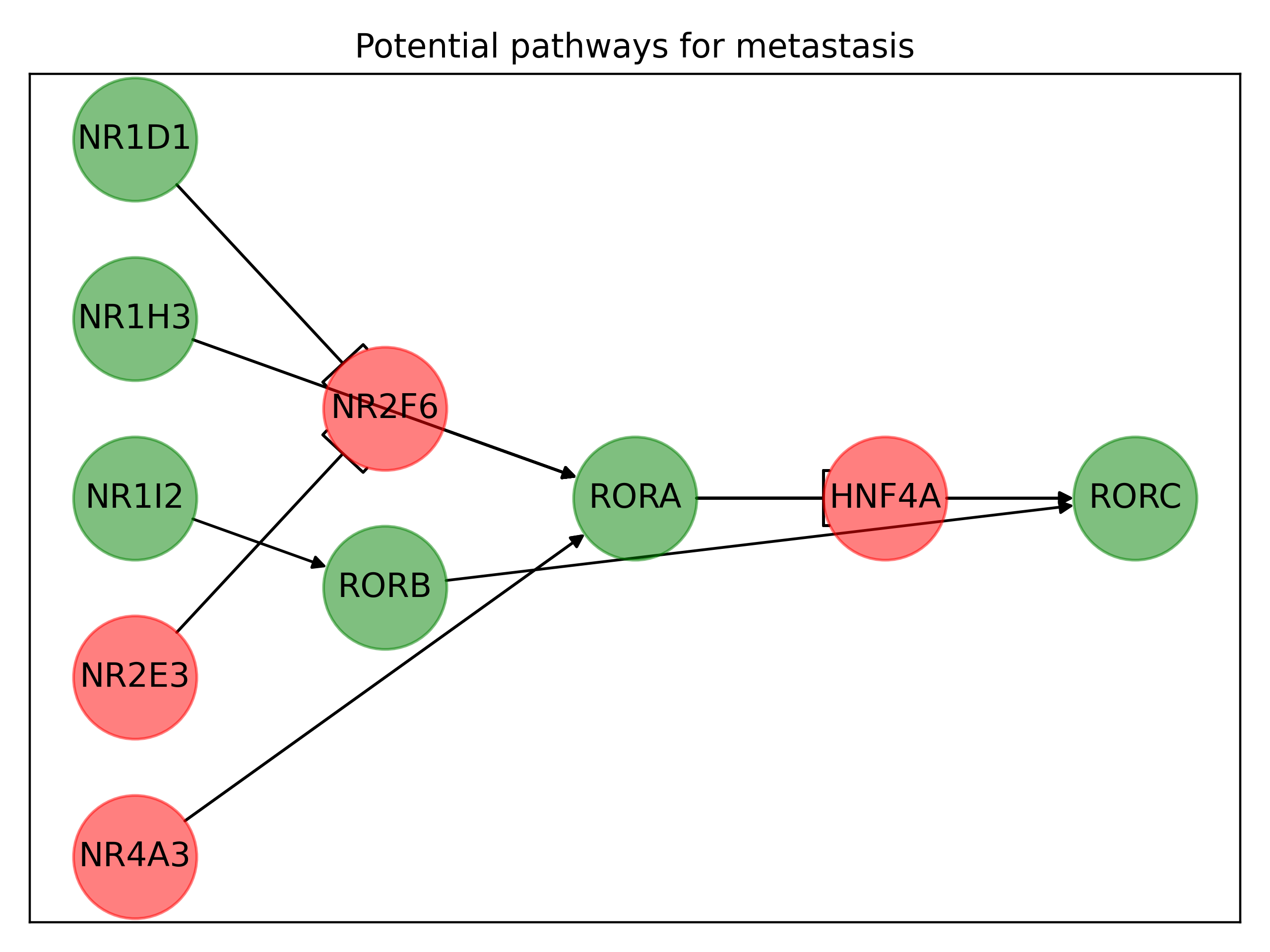
We also show an application of our algorithm to genomic datasets (see Subsection 1.2 for details). We use the reconstructed linear dynamical systems to compute genomic pathways that are prominently different between pathological and reference samples. Thus, unlike standard tools, like [LHA14], that predict genes whose expressions may differentiate between two phenotypes, we can predict pathways that differentiate between two phenotypes. Figure 1, based on the breast cancer RNA-seq dataset [Can12], represents our main contribution in this regard.

Figure 1: Potential pathways for metastasis. Predicted pathways where gene A $\to$ gene B means that A (indirectly) up-regulates B, while the flat arrowhead indicates (indirect) down-regulation. A green node indicates that the corresponding gene expression positively correlates with the pathological phenotype (metastasis), while a red node indicates positive correlation with the reference phenotype. Based on the figure, one prominent pathway could be: NR1I2 up-regulates RORB which up-regulates RORC, whose increased expression is positively correlated with metastasis; based on data in [Can12].

1.1 Relation to filtering

From an abstract algorithmic perspective, the line of work closest to our problem is the Kalman filtering problem in the presence of network loss and delays (see [LXL21], [LWLA20] and [NE19], and the references therein). However, in such results they typically assume a independent identical probability of packet drop or delay, or a specific Markov process of interest is chosen to model that. Also, although the idea of computing conditioned Gaussian distributions (for the error upper-bound in Theorem 3.1) is similar to that used for the analysis of the Kalman filter, the problem studied in our paper differs from the standard filtering problem: (1) we are interested in recovering the underlying linear system and not in predicting the next step of the system, and (2) we are interesting in applications with sparsity (note the connection with compressed sensing).

1.2 Application to genomics

In this subsection we describe an application of Algorithm 1 to the transcriptional regulation problem in genomics. An important problem in genomics is to understand transcriptional regulation – which genes directly regulate a given gene. For example, one version of the problem is to reconstruct Gene Regulatory Networks (GRNs) from gene expression snapshots measured using RNA-seq. The surveys [BiMWMD⁺23] and [BGMN20] cover the tools and techniques employed in the study of GRNs. In particular, in this paper, we model the dynamical system underlying gene expression as a Markov process. Such models have been used to study gene regulation before (see for example [KE01] and [CTSR17]). The paper [KE01] gives a detailed overview of modeling transcription regulation by stochastic differential equations (SDEs); and the Ornstein-Uhlenbeck process that we employ in this paper is just a linear approximation of such SDE models that is analytically tractable and yet expressive enough to capture first order behavior.

Our contribution: Using Algorithms 1, 2 and 3, and the publicly available RNA-seq dataset [Can12]; we have predicted pathways, restricted to nuclear receptors, in Figure 1 that may distinguish between metatstatic and non-metastatic breast cancers. See Sections 2.1 and 4.2 for details.

Note that we do not have the resources to verify the results experimentally, but our predictions may help guide other researchers by narrowing down the genes and pathways for experiments. One way to verify the predictions would be to run our algorithms on a variety of malignant vs control (RNA-seq) datasets and find pathways that are common among the malignant samples. Among the common pathways, one can check for genes that are targets of known drugs, if such drugs exist and they are known to be effective, then they help verify the predictions of our algorithms. Conversely, any genes shared amongst common predicted pathways, that are not yet known, can also be used as targets for newer drugs.

1.2.1 Underlying assumptions and verification

Our algorithms, specifically Algorithm 1, rely on two assumptions: (1) sparsity: the rows of the underlying dynamical system are zero (or near zero) in most entries, and (2) existence of an approximate clock: the ability to (roughly) order our cell samples according to cell age.

Sparsity is usually true because the transcriptional regulation of a given gene directly relies on a handful of polymerases, promoters and previous gene products (see for example [KE01]). Even if we replace direct regulation by downstream regulation within a few steps, for example when studying GRNs restricted to nuclear receptor genes only as opposed to all genes, we would expect this assumption to hold to large extent for the same reasons.

Regarding the existence of an approximate clock, it can be a challenge to find one in datasets. For example, we work with RNA-seq data, which is readily available, unlike single cell RNA-seq data. The disadvantage in using RNA-seq data instead of single cell RNA-seq data is that while it is possible to order cells by their latent time (see for example [hku21]) for single cell data, latent time is not available with RNA-seq data, as latent time is a model based construct. One saving grace is that our algorithms do not use the cell sample ordering except to reconstruct the covariance matrix of increments, which is a pretty robust quantity, and is only significantly effected if the approximate ordering used has too many errors. Therefore, it is possible that using appropriate cyclin expression levels to order cell samples in RNA-seq data, although noisy, may be sufficiently accurate for many datasets.

In this paper, we verify that the reconstructed covariance matrix of increments is indeed robust to a small number of errors in ordering, in three different ways: (1) theoretical justification: we prove that the reconstructed covariance matrix is correct as long as the approximate clock meets certain formal assumptions (Theorem 3.1), (2) by simulation: we use synthetic data to study the error in the reconstructed covariance matrix as function of the number of errors in the approximate clock (Figure 2), and (3) by comparing the approximate ordering based on cyclin expressions with the ordering based on cell latent time in murine pancreatic single cell RNA-seq dataset from [BPSTS⁺19] (Figure 3).

1.2.2 Related problems in genomics

We also note the connection of our approximate cyclin based ordering with the problem of trajectory inference. The trajectory inference problem has been well explored in single cell RNA-seq literature [Sae19], and is likely a harder problem to solve. This is because we only need to order cell samples well enough to approximately recover a specific covariance matrix for the purposes of our algorithms, but in the trajectory inference problem one needs to order the cell samples in the correct sequence to predict cellular development.

Finally, it is possible that cyclin expressions themselves may be effected in many situations by the pathology under consideration (for example [GFKH⁺22]), so while this exact idea may not work in many situations, the basic framework nonetheless should hold.

2 Problem statement and overview

Definition 1

(see for example [Oks13]) Suppose we have a $n$-dimensional Ornstein-Uhlenbeck (OU) process

$$dx_{t}=Bx_{t}dt+AdW_{t},$$ (1)

where $W_{t}$ is $n$-dimensional standard Brownian motion, $A$ is the diffusivity matrix, $AA^{T}$ is the covariance matrix of increments, and $B$ the drift matrix.

Suppose that we observe $x_{t}$ at various time points in $[0,T]$ for large $T$, but we either do not have the ordering information or do not keep the samples ordered. Thus the covariance matrix of the increments of $x_{t}$ is not assumed to be known in this paper, since it requires ordering information for its computation. Then, we want to know whether we can recover the underlying (unknown) $n\times n$ drift matrix $B$, that characterizes our dynamical system.

In general, reconstructing $B$ without ordering information of the $x_{t}$ may not be possible. However, the main technical result in this paper shows that if: (1) there exists an ”approximate clock” (see Definition 2) and (2) $B$ is row sparse, i.e., most of the entries in each row of $B$ are zero or close to zero; then we can approximately reconstruct $B$ with few samples in polynomial time, by solving a convex program.

Definition 2

Given an OU process as in Equation 1, we say that there exists an approximate clock if we know that some subset of the $n$ coordinates of $x_{t}$, or their linear combination, has a positive drift and a relatively smaller diffusivity coefficient.

To keep the presentation simple, we will simply assume that if there exists a coordinate of $x(t)$, denoted by $\tau(t)$, and it is modeled by the diffusion:

$$d\tau(t)=\delta dt+\varepsilon dW^{\prime}_{t},$$ (2)

where $W^{\prime}_{t}$ is standard Brownian motion and $\delta$ is positive and much greater than $\varepsilon^{2}$; then $x(t)$ is said to admit an approximate clock.

Assuming row sparsity of $B$, and the existence of such a clock; our main algorithmic contribution is Algorithm 1, that can recover $B$ from the samples under the assumption that $B$ is row sparse, i.e., each row of $B$ has only $s=\log^{O(1)}(n)$ non-zero entries and the number of samples, i.e., $t$, is larger than $s\log(n)$.

We will use the approximate clock to recover an approximation of the matrix $A$, which we denote by $\tilde{A}$. We won’t actually need $\tilde{A}$ but rather the covariance of the increments: $\tilde{A}\tilde{A}^{T}$; and in Theorem 3.1 in Section 3, we show that ordering the $x_{i}$ values using $\tau(t)$ and computing the covariance from the increments closely approximates the covariance of the increments computed using the ordering based on the actual time.

Algorithm 1 runs in polynomial time as the main steps are computing a covariance matrix and solving the convex optimization problem in Step 7 of Algorithm 1, which is a second order cone program. This convex optimization is a slight variation of basis pursuit in compressed sensing literature (see for example [FR13]) and therefore unique reconstruction is guaranteed under sparsity assumptions. In particular the following uniqueness theorem holds true for the matrix $\tilde{B}$ recovered by Algorithm 1.

Theorem 2.1

[DLR18] Let $s$ denote the row sparsity of $B$, i.e., each row has at most $s$ non-zero coordinates, then for $m=\Omega(\log n)$ large and the sample times for $\{x_{t_{1}},...,x_{t_{m}}\}$ well separated from each other, then we have with probability $1-o(1)$ (for large $n$): $\|\tilde{B}-B\|_{1}=0$, i.e., $B$ can be recovered uniquely by solving a convex program. If however, the rows are not exactly $s$ sparse and the $\ell_{1}$ norm of the $n-s$ remaining entries in any row is at most $\epsilon$, then we have: $\|\tilde{B}-B\|_{1}\leq\epsilon n$.

While the proof follows by easy modifications of known results in existing compressed sensing literature (see [FR13] or [DLR18]), we do note a bit of novelty here over existing compressed sensing literature: the formulation of the constraint in Step 6 of Algorithm 1 uses the characterization of the long term variance of the OU process.

Algorithm 1 recovers the drift matrix $B$ from the covariance matrix $\Sigma$ and the (approximate) covariance matrix of the increments $\tilde{A}\tilde{A}^{T}$ up to an additive factor (that is just the ratio of diffusivity over drift of the approximate clock).

Algorithm 1 Recover dynamical system

1:Input: Unordered snapshots $\{x_{1},...,x_{t}\in\mathbb{R}^{n};t\in[0,T]\}$ derived from an Ornstein-Uhlenbeck process $dx_{t}=Bx_{t}dt+AdW_{t}$; where the diffusivity matrix $A$ is known up to a constant additive error as $\tilde{A}$, and $B$ is row sparse but unknown.

2:Output: A recovered matrix $\tilde{B}$ that is close (in $\ell_{1}$ norm) to $B$.

3:$\triangleright$ Algorithm starts:

4:Compute the $n\times n$ covariance matrix of the random vectors $\{x_{1},...,x_{t}\}$, denoted $\Sigma$

5:$\triangleright$ Note: computing $\Sigma$ does not require ordering the $x_{i}$s.

6:Solve $\tilde{B}:=\arg\min_{B}\sum_{i=0}^{n}\|B(i,\cdot)\|_{2}$      s.t. $\Sigma B+B^{T}\Sigma=-\frac{\tilde{A}\tilde{A}^{T}}{2}$

7:return $\tilde{B}$

Remark 1

Note that the only use of ordering using approximate clock is to recover the matrix $\tilde{A}\tilde{A}^{T}$ in Algorithm 1, we do not use the ordering information anywhere else.

Often it is not enough to recover the drift matrix, but we need to distinguish one linear system from another, where the first is a small perturbation of the second, and one has only few samples of the second at hand. This exact case happens for genomic data samples, where one system is the reference and many samples are available, but another system is some rare genetic condition or disease for which fewer samples are available. Algorithm 2 obtains the perturbation matrix $P$ (within a small error) that distinguishes the second linear system from the first. Note that the algorithm always returns a value for a large enough choice of the noise parameter $\eta$ and small enough choice of $\epsilon$ in Step 8 of Algorithm 2, since that will suffice to make the convex program feasible.

Algorithm 2 Order and recover perturbations between two dynamical systems

1:Input: Unordered snapshots $\{x_{1},...,x_{t}\in\mathbb{R}^{n};t\in[0,T]\}$ and $\{x^{\prime}_{1},...,x^{\prime}_{t^{\prime}}\in\mathbb{R}^{n};t\in[0,T^{\prime}]\}$ derived from two Ornstein-Uhlenbeck processes $dx_{t}=Bx_{t}dt+AdW_{t}$ and $dx^{\prime}_{t}=B^{\prime}x_{t}dt+A^{\prime}dW_{t}$; where the diffusivity matrices $A$ and $A^{\prime}$ are known up to small error, but $B$ and $B^{\prime}$ are unknown. Moreover, $t^{\prime}\ll t$ and $B$ and $B^{\prime}$ are row sparse.

2:Output: A recovered matrix $\tilde{B}$ that is close to $B$ in $\ell_{1}$ norm, and a perturbation matrix $\tilde{P}$ such that $\tilde{B}+\epsilon\tilde{P}\simeq B^{\prime}$, for a small positive parameter $\varepsilon$.

3:$\triangleright$ Algorithm starts:

4:Use Algorithm 1 to compute $\tilde{B}$

5:$\triangleright$ The smaller number of samples prevents direct computation of $\tilde{B^{\prime}}$, so we compute a first order approximation.

6:Compute the $n\times n$ covariance matrix of the random vectors $\{x^{\prime}_{1},...,x^{\prime}_{t^{\prime}}\}$, denoted $\Sigma^{\prime}$

7:$\triangleright$ Choose a small noise $\eta$ so that the following convex program program is feasible

8:Solve $\tilde{P}:=\arg\min_{P}\sum_{i,j=0}^{n}|P_{ij}|$     s.t. $\|(\Sigma-\Sigma^{\prime})\tilde{B}^{T}+\tilde{B}(\Sigma-\Sigma^{\prime})-\epsilon(\Sigma^{\prime}P^{T}+P\Sigma^{\prime})\|_{2}\leq\eta$

9:return $\tilde{P}$

2.1 Algorithm for isolating genomic pathways

As a concrete application, we use the recovered perturbation matrix $\tilde{P}$ to isolate the paths consisting entirely of high weight edges in the directed graph underlying the dynamical system, since these paths should reflect the prominent genomic pathways that differentiate the reference dynamical system from the pathological dynamic system. We note that more standard methods like time series analysis based on Fourier transform of the recovered linear system can also be tried out, but our method below is far simpler, and thus probably more robust to recovery errors, and it suffices to illustrate the pathways that can be recovered.

Intuitively, the matrix $P$ can be thought of as a directed graph with entry $P_{ij}$ reflecting a weighted directed edge from node corresponding to gene $j$ to that for gene $i$. A prominent path is defined to be one such that all its edges have weight higher than some fixed threshold, say $\theta$. For such a prominent path $p$ to potentially reflect an actual underlying genetic pathway that promotes the pathological phenotype, one of the following intuitive condition should hold:

1. If the gene corresponding to the terminal node of $p$ positively correlates with the pathological phenotype then it should be up-regulated by the gene preceding it in the path $p$; moreover, the same property or property (2) should now hold for the subpath terminating in the penultimate gene, and so on.

2. Otherwise, if the gene corresponding to the terminal node of $p$ negatively correlates with the pathological phenotype then it should be down-regulated by the gene preceding it in the path $p$; moreover, the same property or property (1) should now hold for the subpath terminating in the penultimate gene, and so on.

This intuition leads to Algorithm 3 which predicts prominent genomic pathways that may be experimentally verified to confirm that some or all of them lead to the pathological phenotype.

Algorithm 3 Recover Pathways

1:Input: The underlying linear dynamical systems matrices $\tilde{B}$ and $\tilde{B^{\prime}}$ and the correlations between each of the coordinates (corresponding to genes) and the two phenotypes of interest.

2:Output: A set of pathways of a given length $L$ that are prominently different between the two phenotypes.

3:$\triangleright$ Algorithm starts:

4:Compute and sort the list of genes in descending order in terms of the absolute value of their correlation coefficient with the pathological phenotype, denote this list as $\vec{g}$

5:Compute $C:=\mathrm{Diag}(\vec{g})(\tilde{B^{\prime}}-\tilde{B})$

6:Fix a positive threshold $\theta$ and set $C_{ij}=0$ if $C_{ij}<\theta$, denote the resulting matrix as $\Pi_{\theta}$

7:Compute the set of paths of length $L$ in the graph with adjacency matrix $\Pi_{\theta}$ and return them.

The results of running Algorithm 3 on the breast cancer dataset [Can12] to isolate critical differentiating pathways are described in Figure 1. In this figure, we show predicted pathways where gene A $\to$ gene B means that A (indirectly) up-regulates B, while the flat arrowhead indicates (indirect) down-regulation. A green node indicates that the corresponding gene expression positively correlates with the pathological phenotype (metastasis), while a red node indicates positive correlation with the reference phenotype. We show potential pathways, restricted to nuclear receptors, for metastasis. Based on this figure, one prominent pathway could be: NR1I2 up-regulates RORB which up-regulates RORC. Data presented in [Can12] shows that the expression of RORC is positively correlated with metastasis, and thus this pathway is a plausible explanation.

In the rest of the paper we give and prove our main theorem in Section 3 and then give more details on how we obtain the results in Figure 1 in Section 4.1.

3 Theoretical bound on error from approximate clock

In this section, we derive an upper-bound on the error of the recovered diffusivity matrix when we use an approximate clock. We will assume that our dynamical system can be modeled by an OU process and it has a coordinate, or a linear combination of coordinates, that admit a positive drift which is larger than the diffusivity. This coordinate will act as an approximate clock. Theorem 3.1 shows that if we use this approximate clock then the recovered diffusivity is not too different from the diffusivity that would be obtained if we knew the ordering in the dynamical system.

Theorem 3.1

Assuming that the clock coordinate $\tau(t)$ is independent of the remaining coordinates of $x_{t}$, the diffusivity matrix $\tilde{A}\tilde{A}^{T}$ computed using the approximate clock $\tau(t)$ is asymptotically equal to the actual diffusivity, i.e.,

$$\tilde{A}\tilde{A}^{T}=\lim_{h\to 0}\mathbb{E}\left[\frac{1}{\delta T}\int_{0}^{T}\langle(x(\tau(t+h))-x(\tau(t))),(x(\tau(t+h))-x(\tau(t)))\rangle d\tau(t)\right]\simeq AA^{T},$$ (3)

for $\varepsilon\ll\delta$.

Proof

Note that

$$\tilde{A}\tilde{A}^{T}=\lim_{h\to 0}\mathbb{E}\left[\frac{1}{\delta T}\int_{0}^{T}\langle(x(\tau(t+h))-x(\tau(t))),(x(\tau(t+h))-x(\tau(t)))\rangle d\tau(t)\right]$$ (4)

by definition of $x_{t}$. By the tower property of conditional expectation and switching the order of integrals:

$$\mathbb{E}\left[\frac{1}{T}\int_{0}^{T}\langle dx(\tau(t)),dx(\tau(t))\rangle\right]=\mathbb{E}\left[\frac{1}{T}\int_{0}^{T}\mathbb{E}\left[\langle dx(\tau(t)),dx(\tau(t))\rangle\biggr{\rvert}\tau(t)\right]\right]$$ (5)

Recall that,

$$dx(t) = Bx(t)dt+AdW_{t}$$ (6)

$$d\tau(t) = \delta dt+\varepsilon dW^{\prime}_{t},$$ (7)

where $W^{\prime}_{t}$ and $W_{t}$ are independent standard Brownian motions in $\mathbb{R}$ and $\mathbb{R}^{n}$ respectively. The inner conditional expectation can be evaluated in terms of $\tau(t)$ as follows:

$$\mathbb{E}\left[\langle dx(\tau(t)),dx(\tau(t))\rangle\biggr{\rvert}\tau(t)\right]=\mathbb{E}\left[\langle Bx(\tau)d\tau+AdW_{\tau},Bx(\tau)d\tau+AdW_{\tau}\rangle\biggr{\rvert}\tau(t)\right].$$ (8)

Note that we are conditioning a Gaussian with another Gaussian, so the result is a Gaussian variable. The quadratic variation term in the RHS expectation is a sum of three types of terms that can be calculated using:

$$\mathbb{E}\left[\langle AdW_{\tau},AdW_{\tau}\rangle\right] = AA^{T}d\tau(t)$$ (9)

$$\mathbb{E}\left[\langle Bx(\tau)d\tau,Bx(\tau)d\tau\rangle\right] = \varepsilon^{2}Bx(\tau)x(\tau)^{T}B^{T}dt$$ (10)

$$\mathbb{E}\left[\langle AdW_{\tau},Bx(\tau)d\tau\rangle\right] = 0.$$ (11)

The last equality follows because we have assumed that $W^{\prime}_{t}$ and $W_{t}$ are independent. However, that correlation can be calculated explicitly as well, if needed.

Therefore,

$$\int_{0}^{T}\mathbb{E}\left[\langle dx(\tau(t)),dx(\tau(t))\rangle\biggr{\rvert}\tau(t)\right]=\int_{0}^{T}\left(AA^{T}d\tau(t)+\varepsilon^{2}Bx(\tau)x(\tau)^{T}B^{T}dt\right)$$ (12)

Note that

$$\mathbb{E}\left[\frac{1}{\delta T}\int_{0}^{T}AA^{T}d\tau(t)\right]=\mathbb{E}\left[\frac{1}{T}\int_{0}^{T}AA^{T}dt\right],$$ (13)

since the integral with $dW^{\prime}_{t}$ is a martingale with zero mean. Therefore, if $\varepsilon\ll\delta$ then

$$\mathbb{E}\left[\frac{1}{\delta T}\int_{0}^{T}\langle dx(\tau(t)),dx(\tau(t))\rangle\right]\simeq\frac{1}{T}\int_{0}^{T}AA^{T}dt.$$ (14)

$\square$

If the correlations between the randomness in $\tau(t)$ and other coordinates is significant then we can evaluate Equation 11 as follows.

Lemma 1

Let $\rho\in\mathbb{R}^{1\times n}$ be the covariance matrix between $W^{\prime}_{t}$ and $W_{t}$, which are the Brownian motions in the definitions of $\tau(t)$ and $x_{t}$ respectively; then the quadratic variation below evaluates as:

$$\mathbb{E}\left[\langle AdW_{\tau},Bx(\tau)d\tau\rangle\right]=\varepsilon A\rho x(t)^{T}B^{T}dt$$ (15)

The proof follows immediately from the definition quadratic variation. Therefore, following a similar proof as Theorem 3.1, the error to $\tilde{A}\tilde{A}^{T}$ from Theorem 3.1 is changed by an additive factor that is $O(\varepsilon\max\{\rho\})$. So when all coordinates of $\varepsilon\rho$ are small, the characterization of $\tilde{A}\tilde{A}^{T}$ in Theorem 3.1 continues to hold.

4 Empirical bounds on error from approximate clock

Figure 2: Error in determining covariance matrix as a function of the amount of error in the construction of the approximate clock. Note that the Frobenius norm of the difference is small and does not grow too quickly.

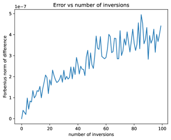
Theorem 3.1 shows that the covariance matrix $AA^{T}$ in Algorithm 1 is determined by an approximate clock as long as $\frac{\epsilon}{\delta}$ is small. In this section we verify the same fact empirically. First, we use synthetic data to plot the error in determining the matrix $AA^{T}$, i.e., $AA^{T}-\tilde{A}\tilde{A}^{T}$, as a function of the number of errors in the cell sample orderings. Note that the latter decreases as $\frac{\epsilon}{\delta}\to 0$. In Figure 2, we plot the Frobenius norm of $AA^{T}-\tilde{A}\tilde{A}^{T}$ as a function of the number of errors in ordering.

In order to generate the plot above, we used an OU process with a $10\times 10$ identity matrix as a stand-in for $A$; we set $B:=-Id+G$, where $G$ is a random Gaussian matrix, and we used time-steps of size $0.0001$ to generate the sample path for $1000$ time-steps. We introduce $k$ errors/inversions (the $x$ coordinate in Figure 2) in the sample path by picking $k$ pairs of points, uniformly at random, in the sample path and swapping the pairs. Finally, we compute $\tilde{A(k)}\tilde{A(k)}^{T}$ from the perturbed path with $k$ inversions, the corresponding Frobenius norm of $\tilde{A(k)}\tilde{A(k)}^{T}-AA^{T}$ and plot the latter as a function of $k$.

4.1 The approximate clock using single cell RNA-seq datasets

(a) Dynamical system obtained from latent time computation

(b) Dynamical system obtained from Cyclin clock

(c) Average entry-wise difference between the recovered dynamical system matrix for various cell clusters

(d) Correlations between various cyclin expressions and scVelo latent time

Figure 3: Effectiveness of Cyclin clock in single cell data

It can be argued that neither Theorem 3.1 nor the verification using synthetic data (Figure 2) uses cyclin expressions. Perhaps using cyclin expressions to order cells leads to a significantly large number of errors in cell sample orderings of RNA-seq data. In this subsection, we allay that fear as well.

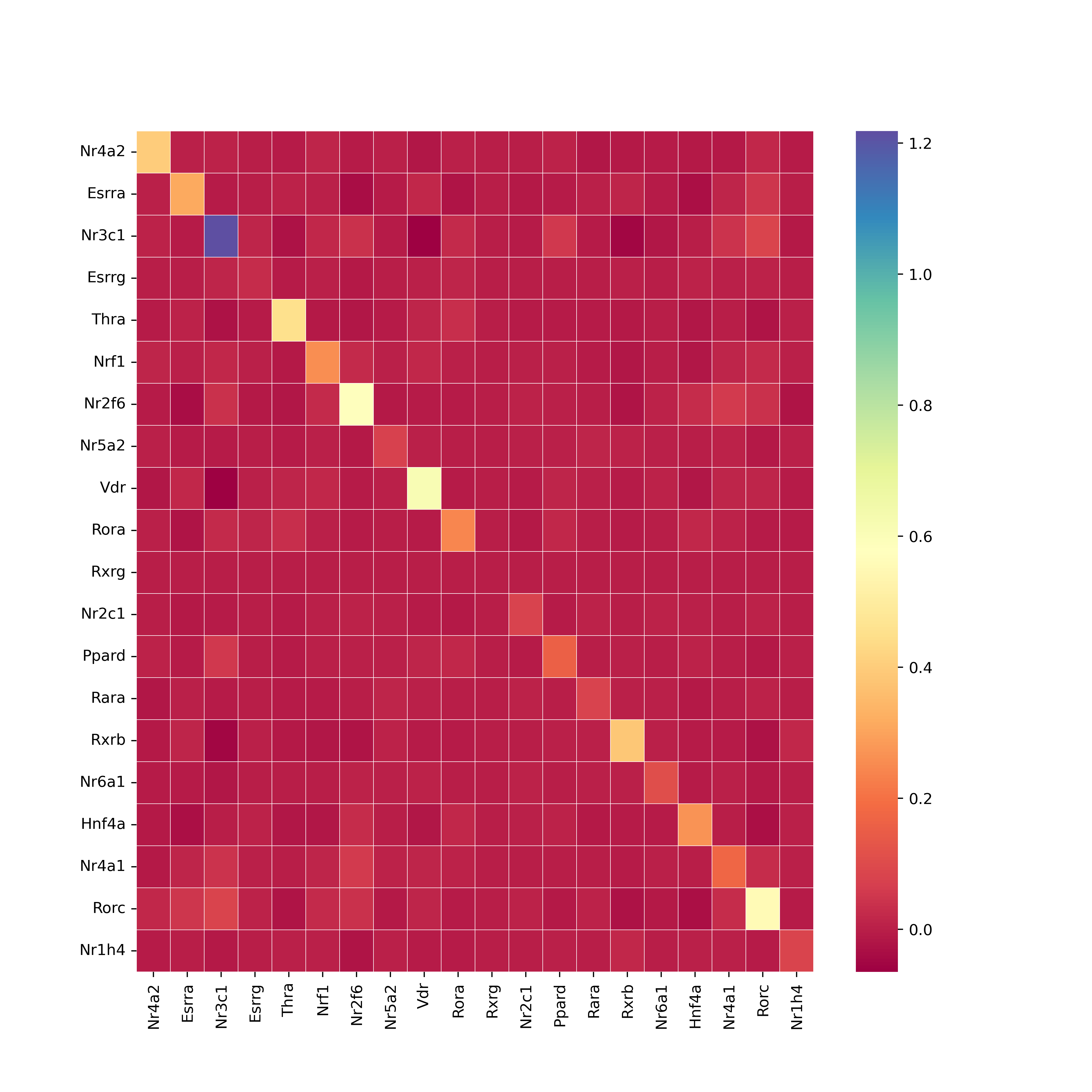
Yet another way to verify that the approximate clock using cyclin expressions does not lead to a large error in determining $AA^{T}$ is to use single cell RNA-seq data. Such datasets admit an ordering of cell samples using latent time using underlying RNA velocity models. In this subsection, we verify that $AA^{T}$ (determined using latent time) and $\tilde{A}\tilde{A}^{T}$ (determined using a simple ordering using cyclin expressions) are close based on single cell RNA-seq dataset from murine pancreatic tissue [BPSTS⁺19].

So we compute the covariance matrix of increments in two ways using the single cell RNA-seq data from [BPSTS⁺19]:

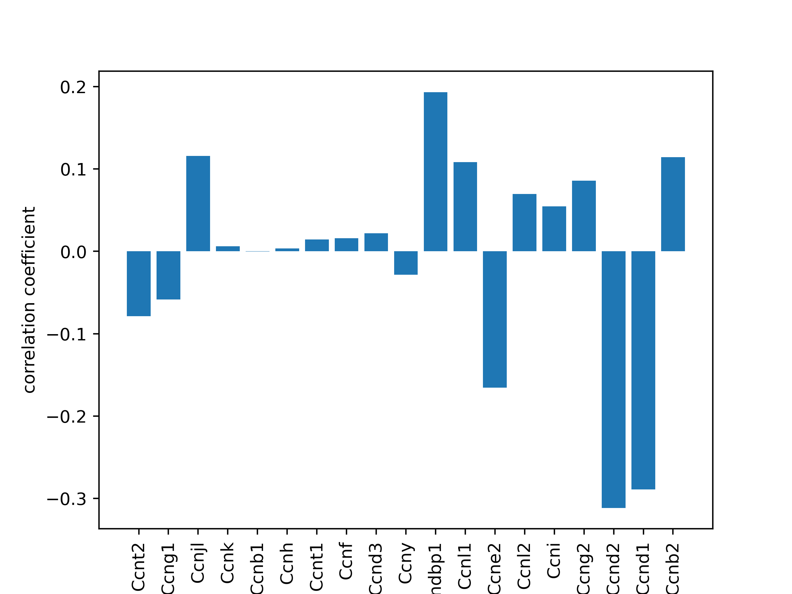
1. First, we compute the matrix $\tilde{A}\tilde{A}^{T}$ using an approximate clock that equals the difference in expression level between two cyclin expressions, say Cyclins I and D, i.e., $\tau(c):=\mathrm{Cyclin\ I}-\mathrm{Cyclin\ D}$ for a given cell $c$. Cyclin I and D represent the optimal choice based on the correlations in Figure 3(d).

2. Next, we compute the diffusivity matrix $AA^{T}$ by using the latent time function in scVelo as our approximate clock.

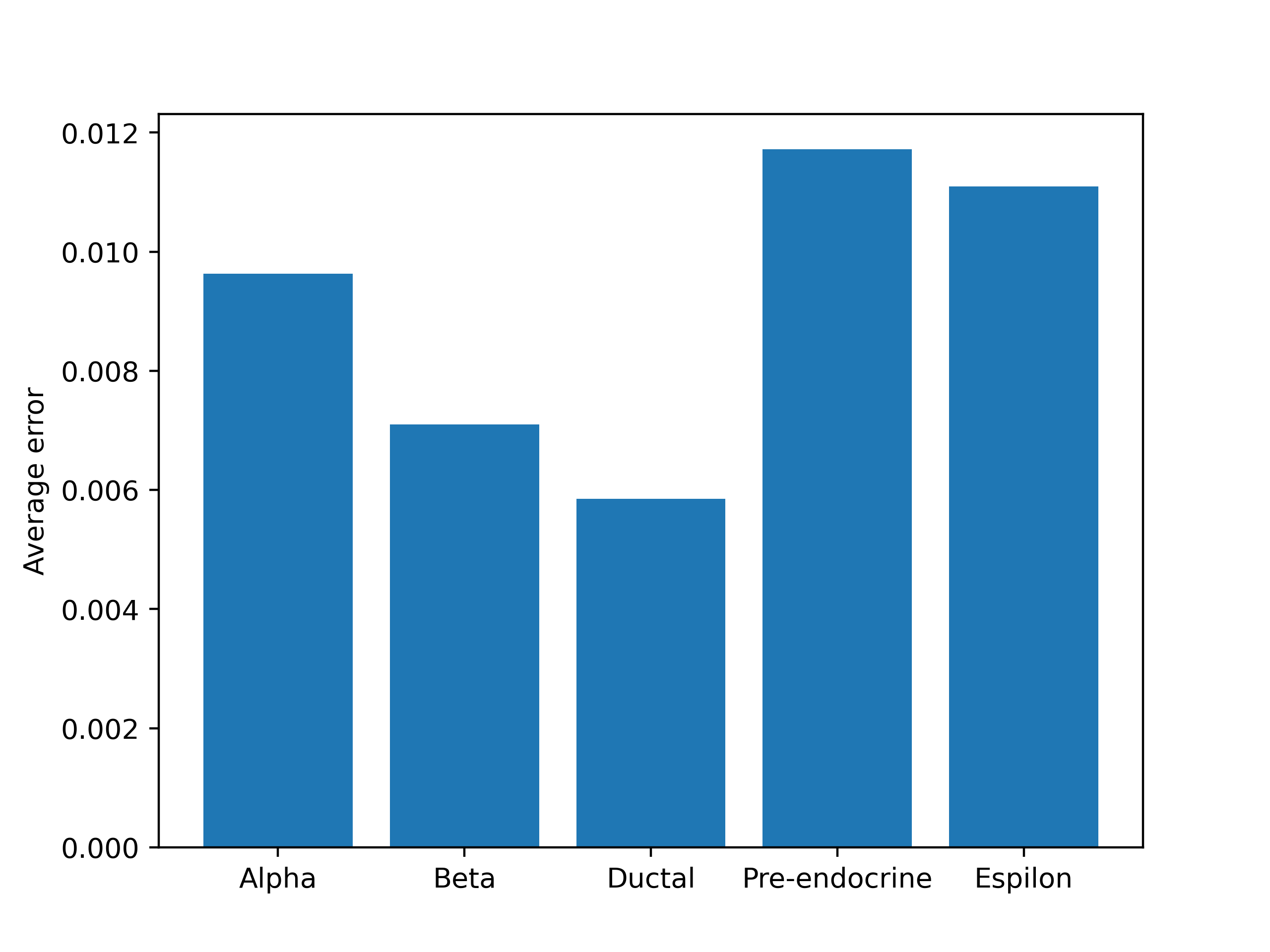
We use the total RNA expression levels data for nuclear receptors in the alpha, beta, epsilon, pre-endocrine and ductal cells in the murine pancreatic single cell RNA-seq dataset [BPSTS⁺19] for this purpose. As can be seen in Figure 3(c), the error measured as the average of entry-wise absolute difference of the computed matrix i.e., $AA-\tilde{A}\tilde{A}^{T}$ is indeed small, much smaller than the variances (diagonals in the heatmaps), thus leading some amount of credence to our overall methods above.

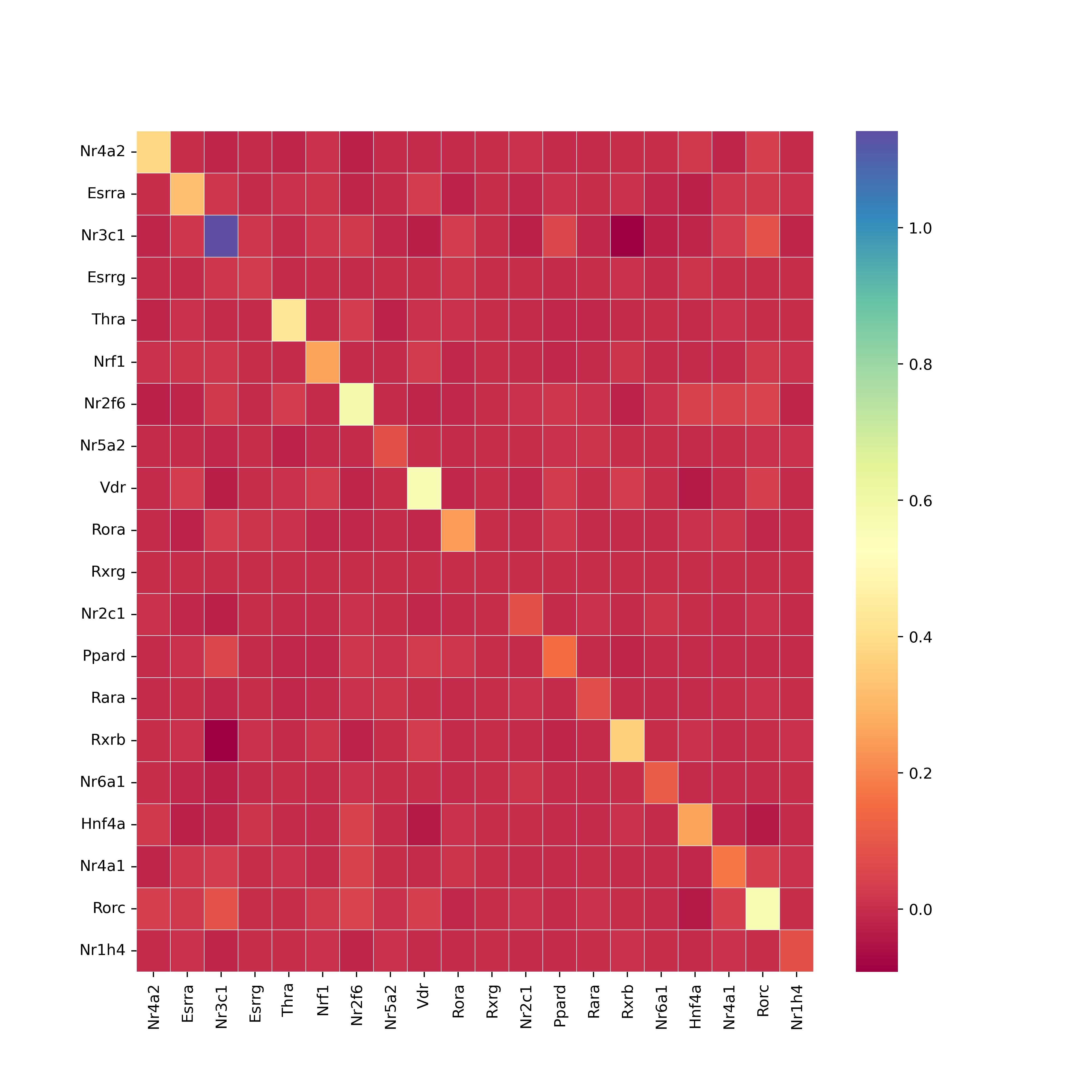
Once we have the approximate clock using cyclin expressions, we can order the cell samples to derive the covariance matrix of increments $\tilde{A}\tilde{A}^{T}$. Finally, we model the logarithmic RNA-seq expression levels in the data-sets [Can12] as an Ornsetin-Uhlenbeck process of the form in Equation 2, and use Algorithm 2 to derive the matrices $\tilde{B}$ and $\tilde{P}$ in Figure 4.

4.2 The reconstructed dynamical system from breast cancer data

(a) Underlying dynamical system for non-metastatic cases

(b) Perturbations towards metastasis

Figure 4: Recovered dynamical system and perturbation for breast cancer dataset.

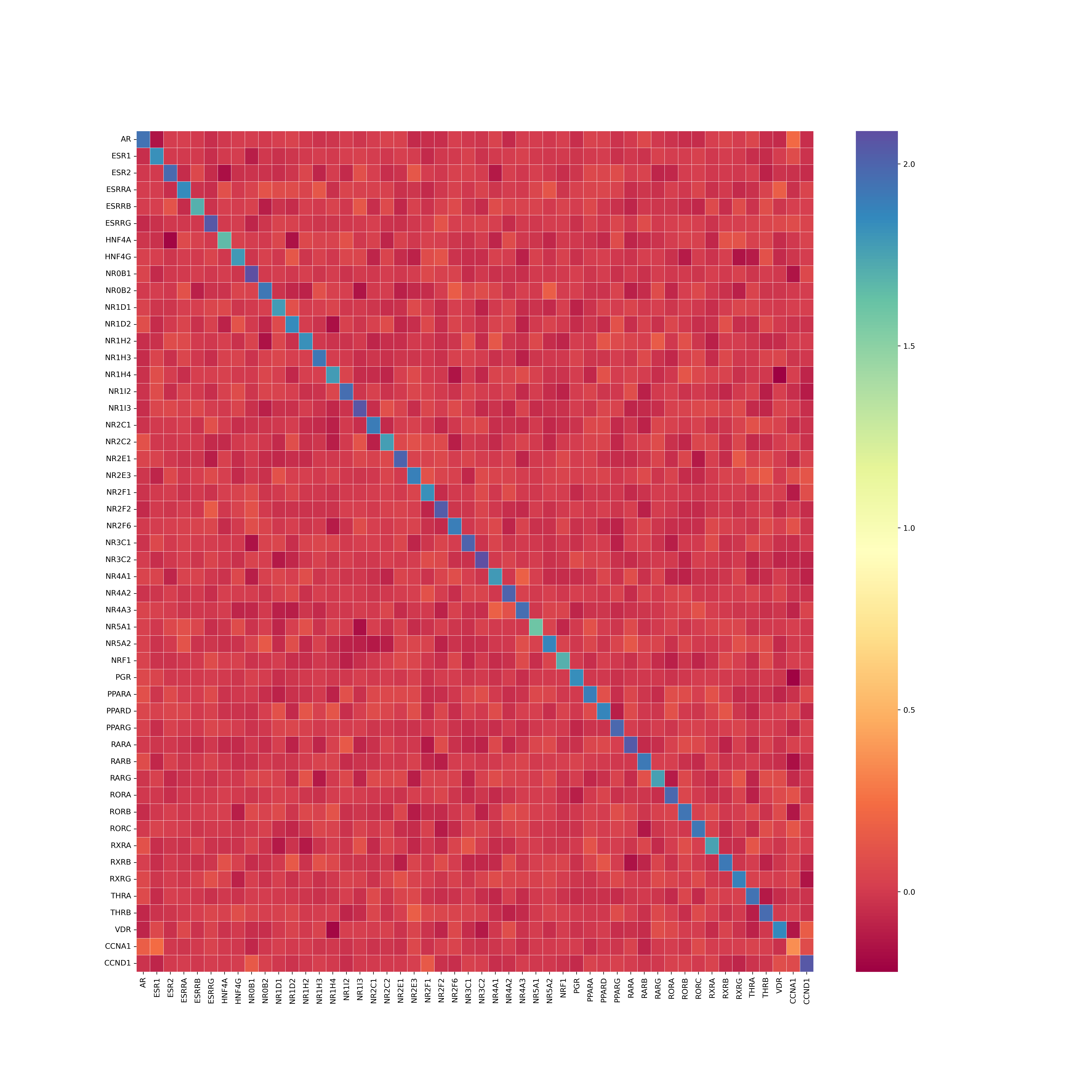
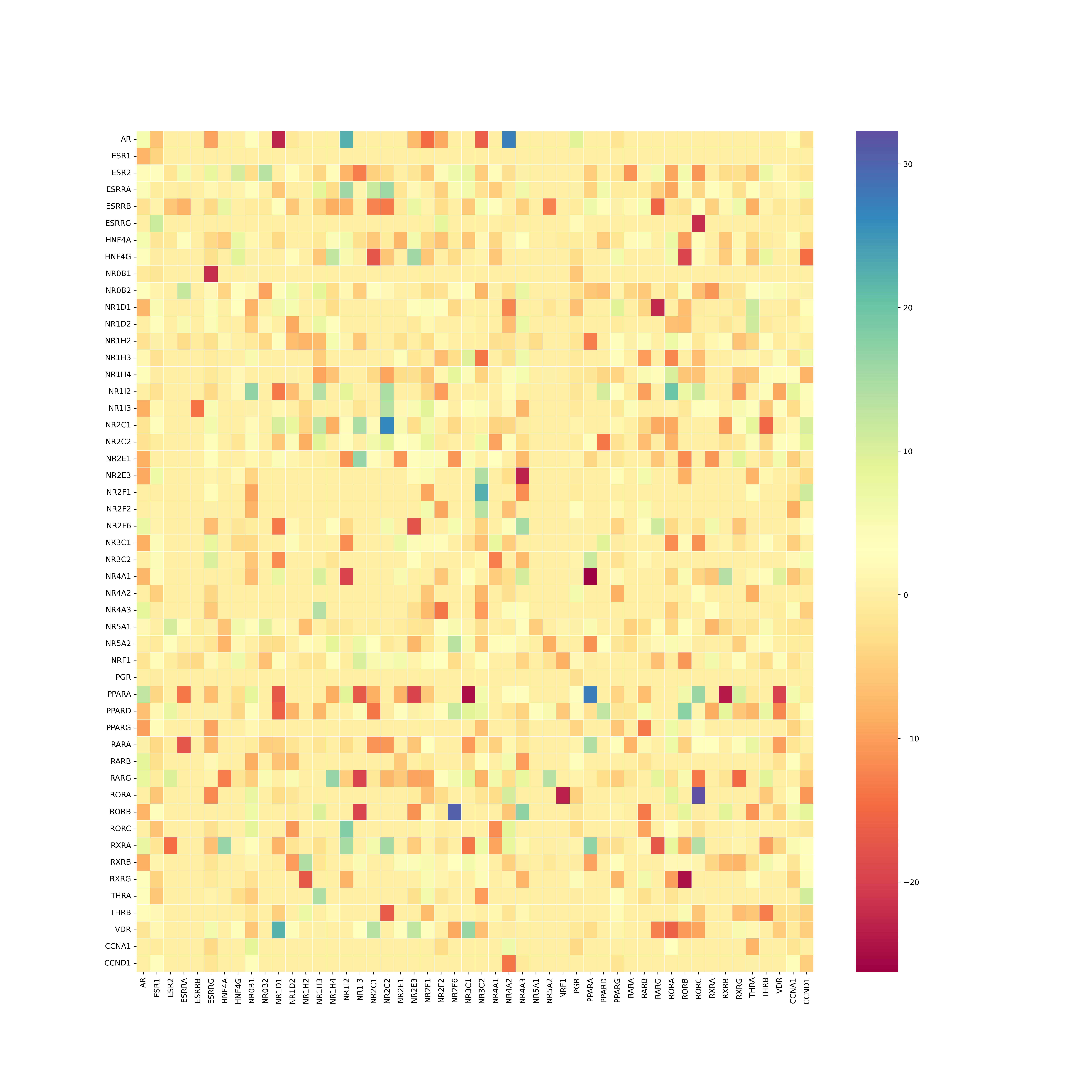
Finally, in order to generate the pathways in Figure 1, we used the publicly available breast cancer dataset [Can12]. First, we used Algorithms 1 and 2 to compute the underlying linear dynamical system matrix: $\tilde{B}$ and the perturbations: $\tilde{P}$, and our results are in the Figure 4. Since the dataset samples are unordered we use a linear combination of cyclin A and D expression levels, as our approximate clock, to order the data-points by cell age. Based on known literature about human cyclins, if we were to obtain a random sample of two cells from a tissue and found the difference, i.e., cyclin A - cyclin D levels, was relatively higher for sample 1 over sample 2 than we know that sample 1 was more advanced in the cell cycle than sample 2 (with some error). Thus we can use their difference in their expression as our approximate clock. Note that we can’t verify how good this clock is, since we don’t have access to any ground truth clock for [Can12] dataset samples that orders cells by their relative cell cycle stage. We used Algorithm 3 on inputs $\tilde{B}$ and $\tilde{P}$ to obtain the pathways in Figure 1.

5 Conclusion

We have demonstrated that it is possible to approximately order the snapshots of a linear dynamical system and reconstruct it from few samples, by combining compressed sensing methods and a simple approximate clock inspired by filtering problems. We have also shown how it can be potentially useful in identifying prominent genomic pathways that differentiate metastatic and non-metastatic samples in a publicly available breast cancer RNA-seq data-set. Due to lack of resources and domain expertise we have not been able to verify the predictions ourselves. However, domain experts should be able to generate and verify such predictions to further their basic understanding of the genomic pathways underlying the conditions.

6 Acknowledgement

The authors are grateful to Dr. Jacob Glass and Prof. S.R.S. Varadhan for helpful discussion and comments.

References

- [BGMN20] Roberto Barbuti, Roberta Guri, Paolo Milazzo, and Lucia Nasti. A survey of gene regulatory networks modelling methods: from differential equations, to Boolean and qualitative bioinspired models. Journal of Membrane Computing, 2:207–226, 2020.
- [BiMWMD+23] Pau Badia-i Mompel, Lorna Wessels, Sophia Müller-Dott, Rémi Trimbour, Ricardo O. Ramirez Flores, Ricard Argelaguet, and Julio Saez-Rodriguez. Gene regulatory network inference in the era of single-cell multi-omics. Nature Reviews Genetics, 24:739–754, 2023.
- [BPSTS+19] Aimée Bastidas-Ponce, Leander Dony Sophie Tritschler, Katharina Scheibner, Marta Tarquis-Medina, Ciro Salinno, Silvia Schirge, Ingo Burtscher, Anika Böttcher, Fabian J Theis, Heiko Lickert, and Mostafa Bakht. Comprehensive single cell mRNA profiling reveals a detailed roadmap for pancreatic endocrinogenesis. Development, 146(12):dev173849, 2019.
- [Can12] Cancer Genome Atlas Network: Daniel C Koboldt et al. Comprehensive molecular portraits of human breast tumours. Nature, 490(7418):61–70, 2012.
- [CTSR17] Brian Chu, Margaret Tse, Royce Sato, and Elizabeth Read. Markov State Models of gene regulatory networks. BMC Systems Biology, 11, 2017.
- [DLR18] Sjoerd Dirksen, Guillaume Lecue, and Holger Rauhut. On the gap between rip properties and sparse recovery conditions. IEEE Transactions on Information Theory, 64(8):5478–5487, 2018.
- [FR13] Simon Foucart and Holger Rauhut. A Mathematical Introduction to Compressive Sensing. Birkhäuser New York, NY, 2013.
- [GFKH+22] Soudeh Ghafouri-Fard, Tayyebeh Khoshbakht, Bashdar Mahmud Hussen, Peixin Dong, Nikolaus Gassler, Mohammad Taheri, Aria Baniahmad, and Nader Akbari Dilmaghani. A review on the role of cyclin dependent kinases in cancers. Cancer Cell International, 22, 2022.
- [hku21] 2021.
- [KE01] Thomas B. Kepler and Timothy C. Elston. Stochasticity in transcriptional regulation: origins, consequences, and mathematical representations. Biophysical journal, 81:3116–3136, 2001.
- [LHA14] Michael Love, Wolfgang Huber, and Simon Anders. Moderated estimation of fold change and dispersion for RNA-seq data with DESeq2. Genome Biology, 15(550), 2014.
- [LWLA20] Dan Liu, Zidong Wang, Yurong Liu, and Fuad Alsaadi. Extended kalman filtering subject to random transmission delays: Dealing with packet disorders. Information Fusion, 60:80–86, 2020.
- [LXL21] Hongjiu Yangand Hui Li, Yuanqing Xia, and Li Li. Distributed Kalman Filtering Over Sensor Networks With Transmission Delays. IEEE Transactions on Cybernetics, 51(11):5511–5521, 2021.
- [NE19] Akram Nikfetrat and Reza Mahboobi Esfanjani. Self-tuning Kalman filter for compensation of transmission delay and loss in line-of-sight guidance. Proceedings of the Institution of Mechanical Engineers, Part G: Journal of Aerospace Engineering, 233(11):4191–4201, 2019.
- [Oks13] Bernt Oksendal. Stochastic Differential Equations: An Introduction with Applications. Springer, Berlin, 2013.
- [Sae19] Saelens, W. and Cannoodt, R. and Todorov, H. et al. A comparison of single-cell trajectory inference methods. Nature Biotechnology, 37:547–554, 2019.