Optimization in Sanger sequencing

Abstract

The main objective of this paper is to solve the optimization problem that is associated with the classification of DNA samples in PCR plates for Sanger sequencing. To achieve this goal, we design an integer linear programming model. Given that the real instances involve the classification of thousands of samples and the linear model can only be solved for small instances, the paper includes a heuristic to cope with bigger problems.

The heuristic algorithm is based on the simulated annealing technique. This algorithm obtains satisfactory solutions to the problem in a short amount of time. It has been tested with real data and yields improved results compared to some commercial software typically used in (clinical) laboratories. Moreover, the algorithm has already been implemented in the laboratory and is being successfully used.

1 Introduction

Recent developments in the study of DNA will have a substantial impact on various fields of science, such as clinical medicine and forensic studies. Increasingly many companies and laboratories are processing DNA samples for various purposes and competing in terms of the time and cost that are required for processing the results. Because optimization techniques can be used to reduce the time or cost of any process, these techniques are of great interest for DNA sample processing.

In this article, we will address a scheduling problem that arises within Health in Code, which is a company that specializes in the genetic diagnosis of inherited cardiovascular diseases. Every day, thousands of DNA samples are processed in their labs.

DNA sequencing is the process that is used to determine the order of the four nucleotides, namely, Adenine (A), Cytosine (C), Guanine (G) and Thymine (T), that make up the DNA molecule. Currently, there are several methods for DNA sequencing. Health in Code is a company that has extensive experience with the Sanger method [7]. The method, which is also referred to as dideoxynucleotide sequencing and chain termination sequencing, consists of the following steps:

• DNA extraction (from samples of tissue, saliva, blood, etc.) and dilution treatment;

• Polymerase chain reaction (PCR): an effective process for making copies of segments of DNA;

• PCR product purification: to remove elements that are used in the PCR process to obtain high-quality DNA samples for sequencing;

• DNA sequencing: to sort the DNA fragments by size in a sequencing machine so that the original piece of DNA can be decoded.

Although all these steps are essential in the Sanger method, this paper focuses on the PCR process. The polymerase chain reaction is a method for amplifying DNA to generate millions of copies of one or several pieces of DNA. To perform this reaction, the DNA is deposited into PCR plates. Then, the plates are placed into thermocyclers to regulate temperature during cyclical programmes.

In this framework, we are interested in optimizing the organization of DNA samples in the plates for performing the PCR process, which is not an easy task since many aspects must be considered to achieve the optimal organization of DNA samples. Each DNA sample is deposited into the well of a plate; however, depending on the components that are used in the procedure, each well from a PCR plate can be used to obtain copies of a single piece of DNA or copies of a group of pieces of DNA. The components that are used with the DNA sample determine not only the piece or pieces to be copied but also the necessary temperature for processing the well in the thermocycler. However, due to the technological characteristics of thermocyclers, wells in the same plate should satisfy several conditions. According to their characteristics, each plate is divided into several strips and all the wells in the same strip should be processed at the same temperature. Moreover, the temperatures of the consecutive strips in the same plate should belong to a specified range.

Since processing each plate in the laboratory is slow and expensive, the main objective of our optimization problem is to order the DNA samples such that the number of plates is minimized under the restrictions that are imposed by the characteristics of the thermocycler. It is also desirable to obtain plates that are as full as possible.

To the best of our knowledge, the optimization literature has not addressed this topic. Characteristics of the problem remind us of a bin packing problem in which samples must be packed in the plates. The bin packing problem is a well-known NP-hard optimization problem (see, for instance, Delorme et al. [3]). For this reason, it is not always possible to obtain the optimal solution of this problem in a reasonable computational time. Some of the heuristic proposals for solving the bin packing problem use strategies that minimize the slack of each bin (see, for instance, Fleszar and Hindi [5]). However, in our setting, if we consider various temperature ranges and the constraints that are associated with the reagent that is necessary for amplifying a specified region of DNA, we will be dealing with a different optimization problem in the end.

Due to the characteristics of our problem, although we have developed an ILP model to solve this problem, we have also implemented a heuristic algorithm based on the simulated annealing procedure that provides satisfactory solutions in short computational times. This algorithm is being successfully used in the laboratory.

The remainder of the paper is organized as follows: In Section 2, the problem is described in detail. Section 3 addresses both the optimization model and the heuristic algorithm. In Section 4, we provide a detailed explanation of the numerical experiments that are necessary for justifying an interest in the results. For this purpose, we have considered real instances from the laboratory.

2 Problem

In this problem, the available DNA samples are organized in PCR plates to be processed in thermocyclers. To perform this task properly, several details must be considered:

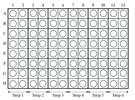
The laboratory uses 96-well PCR plates and the wells are organized in 8 rows and 12 columns. Each plate is composed of six strips. Each strip has 24 wells, which are arranged in 8 rows and 2 columns. According to the characteristics of the thermocyclers, all the wells in the same strip will be processed at the same temperature. In addition, the difference in temperature between two consecutive strips cannot exceed 5 degrees centigrade. Although the strips in a plate must satisfy these temperature conditions, the temperature in the strips is not fixed, but rather is selected by the user. The configuration of a 96-well PCR plate is shown in Figure 1 (a).

(a) empty plate

(b) plate with DNA samples

Figure 1: Example of a PCR plate

Each DNA sample, together with all the chemical components that are necessary for amplifying a specified region of DNA, are deposited in a well. If we are interested in amplifying the same region of DNA for multiple DNA samples, we must include the same chemical components in their corresponding wells. In this case, we say that these DNA samples belong to the same group. All DNA samples in a group must be processed at the same temperature, which is fixed. However, it is possible to have multiple groups with the same temperature.

For instance, let us suppose that the laboratory is interested in studying the risk of genetic diseases. In this particular case, we can think of a group as being associated with a disease. Thus, the laboratory must determine, using the DNA samples of the clients, whether the clients will develop this disease. However, since the disease will be detected by evaluating a specified region of DNA, each DNA sample will be mixed with a reagent and processed at the necessary temperature for amplifying this region.

In addition, one well of the plate should be reserved for the isolated reagent that is associated with a group, which is necessary to verify that the experiment is performed correctly.

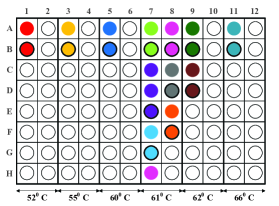
Figure 1 (b) shows an example of one filled plate. The 12 groups are represented by colour. We know the number of DNA samples in each group and the temperatures that correspond to the groups. There are six temperatures for the groups. With this information, we can assign the temperatures in increasing order to the 6 strips of the plate because the temperature difference between any two consecutive strips does not exceed $5^{0}$ C. With this configuration, we have 6 groups that have the same temperature in Strip 4. Moreover, for each group, we have added the reagent, which is represented by a circle of the same colour (but with a black border), as the group samples; see, for instance, the “red” group, which is placed in two wells, one of which contains the DNA sample mixed with the reagent, whereas the other contains only the reagent.

In summary, the laboratory initially has multiple samples, each of which has its own code. The samples belong to groups that are determined by the region of DNA that will be amplified. The laboratory also knows the temperature associated with each group. After solving the optimization problem with this information and the restrictions that are imposed by the characteristics of the PCR plates, we obtain the number of samples of each group in every strip of a plate and whether the reagent of each group is present in any strip. We will also know the temperature of every strip, which will be the only information provided by the optimization problem since in the next phase, the software will place each sample or reagent at random but according to this distribution. Then, for each DNA sample or reagent, we will know the code of the plate and the position where it will be placed, the type of analysis (the group to which it belongs) and the temperature at which it will be processed.

3 Solution methods

3.1 Model

We have designed an integer linear programming (ILP) problem that takes into account all the requirements that were discussed. The main objective of this problem is to minimize the number of occupied plates. We know the number of samples and the temperature for each group. With this information, the ILP problem will assign the samples and the temperature in each strip. Below, we list the parameters and the decision variables that are used in the model.

Parameters:

• $\{1,\ldots,p\}$ is the set of available plates, with index $q$. Because each plate is divided into six strips, the set of strips can be represented by $\{1,\ldots,6\cdot p\}$, with index $l$.

• $w_{q}$ is the weight assigned to each plate $q\in\{1,\ldots,p\}$ in the objective function.

• $\{1,\ldots,n\}$ is the set of groups with index $i$.

• $N_{i}$ indicates the number of samples in each group $i\in\{1,\ldots,n\}$.

• $T_{i}$ is the temperature used in the process for each group $i\in\{1,\ldots,n\}$. Several groups can be processed at the same temperature. Then, we will consider $\{T^{1},\ldots,T^{m}\}\subseteq\{T_{1},\ldots,T_{n}\}$ as the set of temperatures that are used in the process.

Decision variables:

For each strip $l\in\{1,\ldots,6\cdot p\}$, we define the following variables:

• $t_{l}$ is the temperature selected for $l$.

• For each group $i\in\{1,\ldots,n\}$,

  • $n_{il}$ represents the number of samples of group $i$ that are placed in strip $l$.

  • $x_{il}$ is a binary variable such that

    $x_{il}=\left\{\begin{array}[]{ll}1,&\hbox{if the reagent of group $i$ is in strip $l$;}\\ 0,&\hbox{otherwise.}\end{array}\right.$

• For each $j\in\{1,\ldots,m\}$,

  • $y_{jl}$ is a binary variable such that

    $y_{jl}=\left\{\begin{array}[]{ll}1,&\hbox{if strip $l$ has been assigned temperature $T^{j}$;}\\ 0,&\hbox{otherwise.}\end{array}\right.$

Objective function and constraints:

$$\textrm{min }z={\displaystyle\sum_{i=1}^{n}}\quad{\displaystyle\sum_{q=1}^{p}}\quad w_{q}\quad{\displaystyle\sum_{l=6\cdot(q-1)+1}^{6\cdot q}}n_{il}$$ (1)

subject to

$${\displaystyle\sum_{i=1}^{n}}\quad\left(n_{il}+x_{il}\right)\leq 16 \forall l\in\{1,\ldots,6\cdot p\}$$ (2)

$$t_{l}-t_{l+1}\leq 5 \forall l\in\{6\cdot(q-1)+1,\ldots,6\cdot q-1\},\forall q\in\{1,\ldots,p\}$$ (3)

$$t_{l+1}-t_{l}\leq 5 \forall l\in\{6\cdot(q-1)+1,\ldots,6\cdot q-1\},\forall q\in\{1,\ldots,p\}$$ (4)

$${\displaystyle\sum_{j=1}^{m}}y_{jl}\cdot T^{j}=t_{l} \forall l\in\{1,\ldots,6\cdot p\}$$ (5)

$${\displaystyle\sum_{j=1}^{m}}y_{jl}\leq 1 \forall l\in\{1,\ldots,6\cdot p\}$$ (6)

$$y_{jl}\geq\dfrac{{\displaystyle\sum_{i:T_{i}=T^{j}}}n_{il}}{{\displaystyle\sum_{i=1}^{n}}N_{i}} \forall l\in\{1,\ldots,6\cdot p\},\forall j\in\{1,\ldots,m\}$$ (7)

$${\displaystyle\sum_{l=1}^{6\cdot p}}\quad n_{il}=N_{i} \forall i\in\{1,\ldots,n\}$$ (8)

$$n_{il}-x_{il}\geq 0 \forall l\in\{1,\ldots,6\cdot p\},\forall i\in\{1,\ldots,n\}$$ (9)

$${\displaystyle\sum_{l^{\prime}=6\cdot(q-1)+1}^{6\cdot q}}N_{i}x_{il^{\prime}}-n_{il}\geq 0 \forall i\in\{1,\ldots,n\},\forall l\in\{6\cdot(q-1)+1,\ldots,6\cdot q\},$$

$$\forall q\in\{1,\ldots,p\}$$ (10)

$${\displaystyle\sum_{l=6\cdot(q-1)+1}^{6\cdot q}}x_{il}\leq 1 \forall i\in\{1,\ldots,n\},\forall q\in\{1,\ldots,p\}$$ (11)

The objective function (1) minimizes the number of occupied plates. To attain this objective, the number of samples in each plate is multiplied by a weight. Although the laboratory is mainly interested in minimizing the number of plates, it would also be desirable to minimize the total number of occupied cells and maximize, according to the lexicographical order, the occupancy rate of the plates. The three objectives can be accomplished by penalizing the plates in the last positions using the weights. Then, the weights will be considered in increasing order to fill in the cells of the first plates. In practice, we use $w_{q}=q$ for all $q\in\{1,\ldots,p\}$.

Constraint (2) sets the number of available cells in each strip. Constraints (3) and (4) guarantee that the absolute value of the difference in temperature between two consecutive strips does not exceed 5 degrees centigrade. Constraints (5), (6) and (7) ensure that the temperature of each strip is the same as the temperature of the groups with samples in the strip. Therefore, if ${\displaystyle\sum_{j=1}^{m}}y_{jl}=0$, strip $l$ is an empty strip and will not be processed. Otherwise, ${\displaystyle\sum_{j=1}^{m}}y_{jl}=1$ and all the cells in strip $l$ will be processed at the same temperature. Constraint (8) is used to check that all samples are in the cells of the plates, whereas (9), (10) and (11) are associated with the reagent. These last three conditions require that if one or more samples of group $i$ is in plate $q$, the isolated reagent related to this group should be deposited in exactly one well in the plate; otherwise, ${\displaystyle\sum_{l=6\cdot(q-1)+1}^{6\cdot q}}x_{il}=0$ implies that there are no samples of group $i$ in plate $q$ and the corresponding reagent will not appear in the plate.

3.2 Heuristic algorithm

Because it is necessary to provide feasible and reasonable solutions to the problem in a short computational time, we have designed a heuristic algorithm. The heuristic algorithm is based on the simulated annealing method, which was introduced by Kirkpatrick et al. [6]. The main motivation of the simulated annealing method comes from the analogy between the physical annealing of solids and combinatorial optimization problems. A thorough review of this method can be found in Aarts et al. [1] or Eglese [4].

To implement this method, it is necessary to define the problem in terms of a solution space with a defined neighbourhood and cost function. The algorithm starts with an initial solution and moves randomly through the solution space, selecting a neighbour of the current solution and comparing the difference in cost between the two solutions. If the new solution provides a better result in terms of the cost function, we choose it as the new solution. Otherwise, although it provides a poorer result, there is still a probability of accepting the new solution. The probability of accepting a move is typically given by $\exp(-\beta/T)$, where $\beta$ is the cost increment and $T$ is a control parameter that corresponds to temperature in the analogy with physical annealing. According to this probability function, small increases in the cost function are more likely to be accepted than large increases. Moreover, when $T$ is high, most moves are accepted, whereas when $T$ approaches zero, the probability of accepting moves is very small. To avoid local optima, the initial value of $T$ is relatively high and is gradually decreased when new movements are made.

3.2.1 Initial solution

The initial solution is obtained by sorting the groups in ascending order according to their processing temperature. The samples will be deposited by columns in the wells according to this group order. In addition, we must reserve one well for the reagent of the group in all the plates in which at least one sample of the group is deposited. The reagent of a group in a plate will be deposited immediately after the last sample of the group.

Once the samples and reagent of a group have been deposited in the plate, we can deposit the samples of the next group as close as possible, under the restriction that samples of both groups can only be in the same strip if both groups are going to be processed at the same temperature; otherwise, the samples of the two groups cannot be in the same strip.

If the samples of two consecutive groups must be processed at different temperatures, once the samples of the first group have been deposited in the last strip, we deposit the samples of the next group in the consecutive strip if the difference in the processing temperature between the two groups does not exceed $5^{0}$ C. Otherwise, we leave as many empty strips as necessary to satisfy the constraint on the difference in temperature between consecutive strips.

x Input: $samples$, list of samples to be processed; $maxTempDiff$, maximum allowable temperature difference between plate strips

Output: $initialSol$, initial solution (list of plates)

x

1 $plates\leftarrow$ ø

// Samples are sorted according to their temperature (that is, to the temperature of the group

// each of them belongs to)

2 $sort(samples)$

3 for $i=0$ to $samples.size$ do

4       $posPlate\leftarrow 0$

       // Existing plates are traversed to allocate each sample

5       while $posPlate<plates.size$ do

6             $currentPlate\leftarrow plates(posPlate)$

7             $isSampleAssigned\leftarrow\textbf{assignSample}~{}(samples(i),currentPlate,maxTempDiff)$

8             if $!~{}isSampleAssigned$ then

9                   $posPlate~{}+=1$

10                  

11            else

12                   break

13                  

14            

      // Whenever a sample cannot be assigned to existing plates, a new plate is created to contain it

15       if $!~{}isSampleAssigned$ then

16             $newPlate\leftarrow new~{}Plate()$

17             $\textbf{assignSample}~{}(samples(i),newPlate,maxTempDiff$)

18             $addPlate(newPlate,plates)$

19            

20      

21$initialSol\leftarrow plates$

22 return $initialSol$

Algorithm 1 Initial solution

The pseudocode of the algorithm for obtaining the initial solution is presented as Algorithm 1. The main body of the algorithm describes the initial sorting method. Then, the process of assigning a sample to existing plates is performed according to the constraints that are specified above. This process is reflected in the pseudocode in Algorithm 2. If a sample cannot be assigned to an existing plate, a new one is created.

x Input: $sample$, sample to be assigned; $plate$, plate for holding the sample; $maxTempDiff$, maximum allowable temperature difference between plate strips

Output: $true$ if $sample$ is finally allocated in $plate$; $false$ otherwise

x

1

2$isSampleAssigned\leftarrow false$

// First, we attempt to allocate the sample in some of the non-empty strips (that is, strips that already

// hold other samples)

3 $nonEmptyStrips\leftarrow plate.getNonEmptyStrips()$

4 $posStrip\leftarrow 0$

5 while $(!~{}isSampleAssigned~{}~{}\&\&~{}~{}$$posStrip<nonEmptyStrips.size)$ do

6       $currentStrip\leftarrow nonEmptyStrips(posStrip)$

       // A sample can be assigned to a non-empty strip if their temperatures match. There must also be

       // enough space remaining to hold the sample and the reagent of the group (if needed)

7      . if $(\textbf{checkTemperature}~{}(sample,currentStrip)~{}~{}\&\&~{}~{}$$\textbf{checkSpace}~{}(sample,currentStrip))$ then

8             $addSample(sample,currentStrip)$

9             $isSampleAssigned\leftarrow true$

10            

11      else

12             $posStrip~{}+=1$

13            

14      

// If none of the non-empty strips can hold the sample, we try to assign it to some of the

// empty strips (if any)

15 if $!~{}isSampleAssigned$ then

16       $emptyStrips\leftarrow plate.getEmptyStrips()$

17       $posStrip\leftarrow 0$

18       while $(!~{}isSampleAssigned~{}~{}\&\&~{}~{}$$posStrip<emptyStrips.size)$ do

19             $currentStrip\leftarrow emptyStrips(posStrip)$

             // To assign a sample to an empty strip, we must guarantee that the maximum allowable

             // temperature difference between the plate strips is not exceeded

20             if $\textbf{validateTemperatureDiff}~{}(sample,currentStrip,plate,maxTempDiff)$ then

21                   $addSample(sample,currentStrip)$

22                   $isSampleAssigned\leftarrow true$

23                  

24            else

25                   $posStrip~{}+=1$

26                  

27            

28      

29return $isSampleAssigned$

Algorithm 2 Sample assignment

3.2.2 Movements

To improve upon the initial solution and obtain the final positions of the samples in the plates, the main algorithm explores the search space by creating new solutions from a current solution via movements. We have devised two movements, from which a neighbouring solution is generated:

1. Grouping movement. First, a group is randomly selected. If there are samples of the same group in different plates, we randomly choose two plates where at least one sample of the group has been deposited. Then, we try to join all the samples of the group in one of the two plates. If the empty wells in the plate are not sufficient for this, it is possible to move to the plate samples of other groups that have similar processing temperatures. The groups that have samples in the other plate are preferred to other groups. Moreover, we move the minimum number of plates that are necessary to satisfy the feasibility constraints. This movement also allows all the samples of one group to be moved from one plate to another plate where there is no sample in the group.

2. Strip-exchange movement. We select two strips in two plates and exchange them. Although the temperature constraint between consecutive strips should be satisfied for the movement to be permitted, the temperatures of the strips can be different.

The movements will be selected according to a fixed parameter that denotes the probability of each movement. If a movement is not feasible, a new movement will be made. If no movement is feasible, the algorithm terminates and the solution that was obtained in the last iteration is selected as the final solution of the algorithm.

3.2.3 Cost function

The cost function for comparing the current and new solutions at each iteration of the algorithm is obtained by applying the lexicographical order to the following objectives:

• First objective: minimize the number of non-empty plates.

• Second objective: minimize the number of non-empty wells.

We only used two objectives because the definition of the implemented movements and the second objective indirectly improve the occupancy rate of the plates. Furthermore, we could have considered a single objective, as in the ILP model. However, the use of a single aggregated objective often results in the heuristic algorithm finding local minima and in a high degree of variability in the results. Thus, we have ruled out this strategy.

The pseudocode of the algorithm for obtaining the final solution is presented as Algorithm 3.

x Input: $initialSol$, initial solution; $maxIter$, maximum number of algorithm iterations; $Tmax$, initial temperature; $Tmin$, minimum temperature; $\alpha$, cooling parameter; $SEProb$, probability of applying a $Strip-exchange$ movement (thus, a $Grouping$ movement will be applied with probability $1-SEProb$)

Output: $bestSol$, best global solution that has been found

x

1

2$bestSol\leftarrow initialSol$

3 $currentSol\leftarrow initialSol$

4 for $i=0$ to $maxIter$ do

5       $T\leftarrow Tmax$

6       while $T\geq~{}Tmin$ do

             // A new solution is created from the current one by applying a movement. If

             // no movement can be applied, the algorithm terminates

7             $newSol\leftarrow\textbf{applyMovement}~{}(currentSol,SEProb)$

8             if $newSol=$ ø then

9                   return $bestSol$

10                  

11            else

                   // We must always keep updated the best global solution that has been found so far

12                   $updateBestSol~{}(newSol,bestSol)$

                   // If $newSol$ improves $currentSol$ (that is, if it uses fewer plates or

                   // if it minimizes the number of non-empty wells), it will replace the current solution

                   // for the next iteration

13                   case $\textbf{numPlates}~{}(newSol)<\textbf{numPlates}~{}(currentSol)$ do

14                         $currentSol\leftarrow newSol$

15                  

16                  case $\textbf{numPlates}~{}(newSol)=\textbf{numPlates}~{}(currentSol)$ do

17                         if $\textbf{nonEmptyWells}~{}(newSol)\leq\textbf{nonEmptyWells}~{}(currentSol)$ then

18                               $currentSol\leftarrow newSol$

19                        else

20                               $threshold\leftarrow e^{\frac{nonEmptyWellsDiff(newSol,currentSol)}{T}}$

21                               $\textbf{acceptWorseSolution}~{}(generateRandom(),threshold,newSol,currentSol)$

22                              

23                        

                  // Even when $newSol$ is worse than $currentSol$, it still may replace the current solution

24                   otherwise do

25                         $threshold\leftarrow e^{\frac{numPlatesDiff(newSol,currentSol)}{T}}$

26                         $\textbf{acceptWorseSolution}~{}(generateRandom(),threshold,newSol,currentSol)$

27                        

28                  

29            $T\leftarrow\alpha*T$

30            

31      

32return $bestSol$

33

Algorithm 3 Simulated annealing

3.2.4 Example

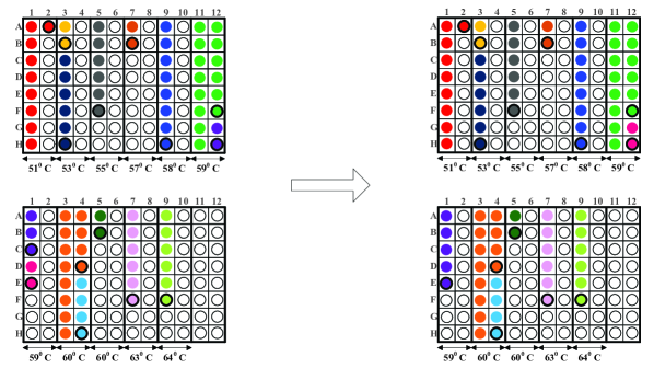
To demonstrate how the algorithm operates, we consider the following example: We must distribute 69 samples that are organized in 14 groups (and the corresponding reagents) in the plates. The initial solution of the algorithm is represented in the first part of Figure 2. The groups are ordered according to their temperatures in increasing order. According to this order, we fix the temperatures of the strips. To organize the samples under this criterion, we need two plates and the number of occupied cells is 84 (69 samples and 15 reagents). There are several strips that have the same temperature since in these cases, one strip is not sufficient to hold all the samples that are processed at the corresponding temperature. Moreover, the samples of the “violet” group are distributed in both plates. Then, the grouping movement could consist of joining all the samples of the group in the first plate and moving the “pink” group to the first plate.

Both solutions (the initial solution and the solution obtained after 1 iteration of applying the grouping movement of the algorithm) require two plates. However, whereas the number of occupied cells in the initial solution is 84, this number is reduced to 83 after 1 iteration since the number of reagents has been reduced from 15 to 14. Thus, the solution has been improved after 1 iteration.

Figure 2: Grouping movement

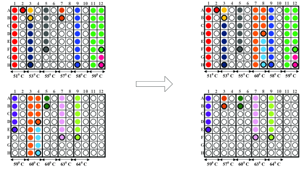
Suppose we accept this new solution and perform another iteration. Now, we could apply the strip-exchange movement on the fourth strip of the first plate and the second strip of the second plate. After this movement, the number of occupied cells is again 83; however, the solution is improved because the occupancy rates have changed from (51.04,35.42) to (65.63,20.83). This movement is illustrated in Figure 3.

Figure 3: Strip-exchange movement

4 Experimental results

4.1 Data

The solution methods have been tested with real data. We have considered 36 files, which are divided into two sets:

• The first set contains 30 files (Id 1-30), each of which contains information on one working session in the laboratory.

• The second set contains 6 files (Id 31-36). Each one of these files corresponds to 2 or 3 plates that have been randomly chosen from one working session.

Table 1 summarizes the main characteristics of the files (numbers of samples, groups and group temperatures). In both sets, the files have been ordered according to the number of samples. The number of temperatures remains stable in all scenarios. However, the number of groups and, especially, the number of samples vary considerably. Hence, the characteristics of each working session are highly particular.

Id	1	2	3	4	5	6	7	8	9	10	11	12
Samples	174	193	233	285	290	315	358	368	432	434	501	551
Groups	80	68	31	147	87	99	35	27	32	44	82	37
Temperatures	13	14	12	18	10	16	10	11	14	13	15	15
Id	13	14	15	16	17	18	19	20	21	22	23	24
Samples	612	647	747	797	876	918	963	1128	1270	1309	1398	1473
Groups	107	27	37	27	120	184	37	192	167	201	200	197
Temperatures	17	12	15	11	13	17	15	16	17	17	18	16
Id	25	26	27	28	29	30	31	32	33	34	35	36
Samples	1944	2071	2248	2496	2703	3783	40	44	50	65	77	84
Groups	151	162	165	179	200	171	24	31	45	34	43	68
Temperatures	15	15	17	17	17	17	11	11	14	15	13	16

Table 1: Description of the files that were obtained from real data

4.2 Comparison between LabWare, the ILP model and the heuristic algorithm

This section is devoted to comparing the results that were obtained in the laboratory with LabWare software and the results that were obtained via our solution methods. Our solution methods have been evaluated using a computer with an Intel(R) Core(TM) i7-3770 CPU of 3.40 GHz and 16 GB of RAM. Moreover, the ILP problem was solved using Gurobi Optimizer (version 6.0.5), whereas the heuristic algorithm was implemented in Java.

Each working session in the laboratory involves many samples and groups. Thus, the ILP problem for Files 1-30, which are related to real working sessions, will be large and cannot be solved in a reasonable amount of time. To demonstrate this, Table 2 lists the results that were obtained with ten examples from the first set. The ILP problem solutions were obtained after 60 hours. According to Table 2, after this time, we cannot guarantee the optimality of the solutions. The table also indicates the best solution that was obtained and the size of the ILP problem, the gap of the solution and the minimum time needed to obtain the solution. The results demonstrate the necessity of developing a tool to identify satisfactory solutions in a reasonable computational time.

Id	ILP problem solution
	Plates	Occupancy rates	Size	Gap (%)	Minimal time
1	4	100/98.96/44.79/22.92	4664$\times$4176	2.17	2.07 h
2	5	100/97.92/55.21/20.83/2.08	5048$\times$4530	3.14	0.21 h
3	4	100/94.79/64.58/26.04	2043$\times$1800	4.17	54.87 h
4	7	98.96/97.92/96.88/95.83/39.58/17.71/6.25	14476$\times$13146	5.43	59.61 h
5	5	100/100/100/72.92/22.92	6182$\times$5550	1.18	12.89 h
6	6	100/100/96.87/84.37/46.87/6.25	7989$\times$7452	1.02	3.46 h
7	5	100/100/100/80.20/36.46	2750$\times$2430	0.99	58.21 h
8	5	100/100/98.96/86.46/31.25	2252$\times$1980	1.90	53.8 h
9	7	100/100/100/98.96/65.63/23.96/2.08	3364$\times$3318	1.90	41.05 h
10	7	100/100/98.96/98.96/75.00/28.13/4.17	4790$\times$4284	1.79	45.92 h

Table 2: Solutions for Files 1-10 that were obtained by solving the ILP problem

However, it is possible to find the optimal solutions in few seconds for problems that are associated with a small number of plates. For this reason, we have considered 6 small examples with 2 or 3 plates that are configured in the laboratory with LabWare. Despite not being representatives of a typical working session, these examples will be useful for comparing optimal solutions with the solutions that are provided by the heuristic algorithm. Thus, in Table 3 we can compare the occupancy rates of the three methods: LabWare, the ILP model and the heuristic algorithm. The table also lists the computational times for the ILP model and the heuristic algorithm.

Id	Occupancy rates				Computational times
	LabWare	ILP model	Heuristic		ILP model	Heuristic
31	37.50/29.17	50.00/16.67	50.00/16.67		0.01 s	0.006 s
32	29.17/28.13/20.83	57.29/20.83	57.29/20.83		0.25 s	0.07 s
33	54.17/37.50/7.29	71.88/20.83/6.25	71.88/20.83/6.25		0.88 s	0.065 s
34	41.67/39.58/21.88	73.96/20.83/8.33	73.96/20.83/8.33		4.04 s	0.26 s
35	47.92/47.92/30.21	86.46/32.29/6.25	86.46/32.29/6.25		4.76 s	0.55 s
36	67.71/50.00/40.63	91.67/45.83/20.83	91.67/45.83/20.83		4.76 s	0.62 s

Table 3: Examples with 2 or 3 plates

We have obtained the optimal solutions of the ILP problem in Files 31-36. However, the solution provided by LabWare never coincides with the optimal solution. In the second example, the LabWare solution requires an additional plate and in the other cases, the distribution of the samples in the plates is worse. However, after determining the best values for the input parameters in the algorithm (a study of the parameters of the algorithm will be performed next), we have verified that for these $2$ and $3$ plate files, the heuristic algorithm reaches the optimal value provided by the ILP model in less time. Since Files 31-36 have been randomly selected from the same working session, these results enable us to guarantee the satisfactory performance of the heuristic algorithm.

4.3 Study of the parameters in the heuristic algorithm

In this section, we focus on obtaining the appropriate parameters for Algorithm 3 according to our experimental environment.

The algorithm depends on several input parameters, as discussed above. To ensure its proper performance in our scenario, it is necessary to adjust these parameters according to our data. Next, we justify the values of these input parameters:

• Initial temperature. The initial temperature was set to 100. According to Ben-Ameur [2], this value ensures a low probability of acceptance of poor solutions with respect to the first objective and higher acceptance ratio with respect to the second objective. Thus, when the number of plates is minimized, there is greater flexibility for filling them in the best possible way.

• Minimum temperature. The final temperature at each simulated annealing iteration was set to $1E-10$. This low value permits an exhaustive search at each iteration.

• Cooling parameter ($\alpha$). Our annealing procedure initially considers a high temperature. Then, the temperature is lowered incrementally by a constant factor. It is important to consider sufficiently many steps at each temperature to keep the system close to equilibrium until the system approaches the minimum temperature. We have considered $\alpha=0.9$.

• Maximum number of iterations. Once the above parameters were set, we performed an exhaustive study of the execution times by varying the number of iterations. According to the results of this study, a value of 1000 iterations has been chosen to ensure a reasonable execution time in all scenarios. In addition, the objective function values of the problem do not improve after 1000 iterations.

• Probability of the $Strip$-$exchange$ movement, which is the parameter that most influences the result of the algorithm. We have studied the results that were obtained for all files by varying the probability of choosing this movement from $0$ to $1$ in increments of $0.1$. According to this empirical study, this movement is the more effective of the two implemented movements as it obtains only the best solutions if a high probability has been assigned to it.

  For simplicity, Table 4 lists the results for probability values of $0.8$, $0.9$ and $1$. To summarize the results for each instance, Table 4 lists the minimum number of plates that are required for placing the samples, the total number of full plates and the fill rate of the first plate that is not filled. The $Grouping$ movement plays no role in small instances, as poorer results are always obtained when it is involved. However, for larger files, it is important to apply it with low probability to obtain the best results. For instance, in File $27$, we can obtain $24$ full plates out of a total of $27$ by assigning probability $0.2$ to the $Grouping$ movement and probability $0.8$ to the $Strip$-$exchange$ movement.

  

  

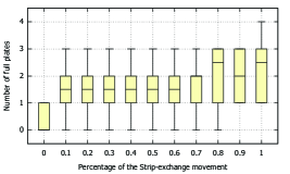
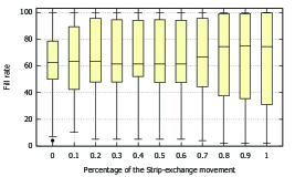
  Figure 4: Study of the Strip-exchange movement for small instances (Files 1-10)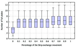

  

  

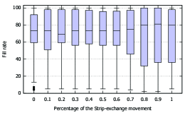
  Figure 5: Study of the Strip-exchange movement for medium instances (Files 11-20)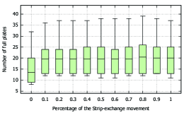

  

  

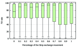
  Figure 6: Study of the Strip-exchange movement for large instances (Files 21-30)

  Figures 4, 5 and 6 show the fill rates that were obtained for various probabilities of the $Strip$-$exchange$ movement in small, medium and large instances, respectively. Figures 4, 5 and 6 support the following observation from Table 4: the probabilities of 0.8 and 0.9 for the $Strip$-$exchange$ movement yield the best filling rates for medium and large working sessions.

  Id	Plates	Full plates			Percentage
  		0.8	0.9	1	0.8	0.9	1
  1	4	1	1	1	96.88	97.92	98.96
  2	5	1	1	1	91.67	86.46	95.83
  3	4	0	1	1	97.92	80.21	80.21
  4	7	1	1	2	97.92	97.92	97.92
  5	5	2	2	3	91.67	91.67	75
  6	6	3	2	2	85.42	93.75	98.96
  7	5	3	3	3	80.21	80.21	81.25
  8	5	3	3	3	85.42	84.38	86.46
  9	7	3	3	4	94.79	96.88	39.58
  10	7	3	3	4	95.83	95.83	63.54
  11	8	5	5	5	54.17	79.17	76.04
  12	8	5	5	5	84.38	79.17	73.96
  13	9	4	4	5	98.96	98.96	91.67
  14	9	6	6	6	83.33	85.42	78.12
  15	10	6	6	6	98.96	98.96	91.67
  16	10	7	7	6	94.79	89.58	97.92
  17	12	8	8	8	98.96	98.96	97.92
  18	13	8	8	8	95.83	98.96	95.83
  19	12	9	9	8	89.58	94.79	93.75
  20	15	12	12	10	86.46	96.88	96.88
  21	17	13	13	11	85.42	93.75	97.92
  22	18	12	13	12	98.96	98.96	98.96
  23	19	13	13	13	95.83	97.92	88.54
  24	19	14	15	14	97.92	82.29	97.92
  25	23	20	19	19	93.75	98.96	83.33
  26	25	21	21	21	98.96	98.96	93.75
  27	27	24	23	21	76.04	97.92	85.42
  28	30	26	25	25	98.96	94.79	93.75
  29	32	29	28	28	87.5	96.88	86.46
  30	44	39	38	37	98.96	86.46	96.98

  Table 4: Results of applying the $Strip$-$exchange$ movement with probabilities $0.8$, $0.9$ and $1$

4.4 Final results

Once the parameters of the algorithm have been chosen, we will compare the results that were obtained by applying the heuristic algorithm with those that were obtained in the laboratory using the LabWare software for Files 1-30.

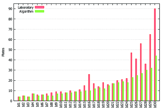
The first and most important objective is the reduction of the number of plates necessary to process the samples. Figure 7 shows the number of plates that are saved by the heuristic algorithm compared to the solution that was provided by the LabWare software. In view of Figure 7, it is evident that the heuristic algorithm is able to provide better solutions in most of the files. The savings are more significant in large instances.

Figure 7: Comparison between the total number of plates that were obtained via the LabWare software and the heuristic algorithm

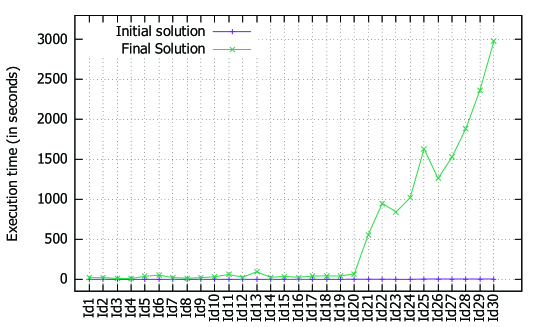
In addition, the heuristic algorithm achieves the solutions in reasonable times for the laboratory, as shown in Figure 8. It is also provided a comparison of the times necessary for the heuristic algorithm to obtain the initial and final solutions. The initial solution is calculated in few seconds for all working sessions, whereas the computational time of the final solution depends to a large extent on the number of samples of each file.

Figure 8: Comparison of the times in which the initial and final solutions of the algorithm are obtained

As it has been previously mentioned, it is also interesting for the laboratory to have a certain distribution of the plate occupancy rates, so that the first plates are more occupied than the last plates. This would allow new samples to be placed on the most empty plates, which have not yet been processed, as these are the ones that occupy the last positions. Figure 9 and Figure 10 show the distribution of the plate occupancy with the algorithm and Labware in small and medium instances, respectively.

Figure 9: Distribution of the plate occupancy obtained with the algorithm and LabWare in small instances

Figure 10: Distribution of the plate occupancy obtained with the algorithm and LabWare in medium instances

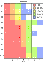
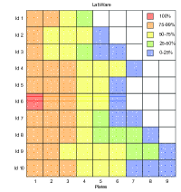
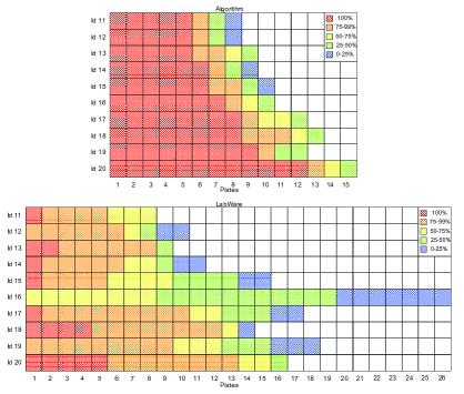
In the case of both figures, each row represents the best solution obtained for the corresponding instance by the proposed algorithm and by LabWare. The coloured squares represent the occupied plates and the occupancy level (100%, [75,100)%, [50,75)%, [25,50)% and [0,25)%) is indicated by the different colours. It can be clearly seen that both the number of plates used and the number of full plates is worse in the solution obtained by LabWare.

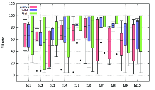
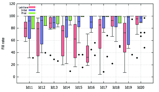
To highlight the efficiency of the heuristic algorithm against the solution that was obtained with LabWare, Figure 11 compares, by means of box-plots, the fill rates that were obtained by the initial and final solutions of the algorithm with the ones provided by LabWare for small and medium instances (Files 1-20). In the case of the medium instances, the solutions of the algorithm yield much higher fill rates than LabWare’s solution.

Figure 11: Comparison of the fill rates that were obtained by LabWare, the initial solution, and the final solution of the algorithm

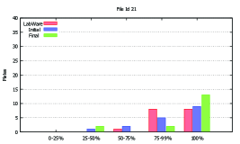
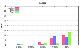
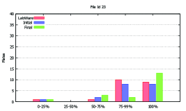
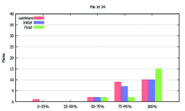
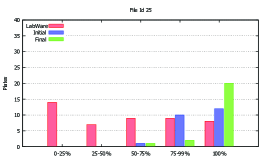
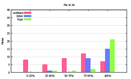
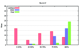
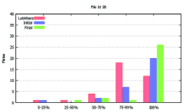
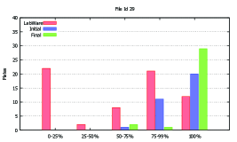
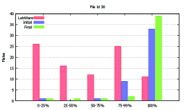
Finally, Figure 12 compares the filling distributions of initial and final solutions that were obtained via the heuristic algorithm with the solution provided by LabWare for large instances (Files 21-30). As a summary of the obtained results, the number of plates that correspond to each range of filling percentages (100, [75,100), [50,75), [25,50) and [0,25)) is displayed for each file. Thus, for instance, in the case of the largest file (Id $30$), the heuristic algorithm finds a scheme that fills $39$ plates out of a total of $44$ plates, while the LabWare solution fills $11$ plates out of a total of $90$.

Figure 12: Distribution of the plate occupancy obtained with the initial and final solutions of the algorithm and LabWare in large instances

Concluding remarks

In this paper, a real problem that was proposed by Health in Code is studied. This company specializes in genetic diagnosis services for cardiovascular diseases. One of the diagnosis procedures is based on the Sanger method. The Sanger method consists of several phases. In one phase, DNA samples are placed into PCR plates to be processed in thermocyclers. The problem addressed in this paper focusses on the organization of samples in plates such that the minimum number of plates are used since plate processing is expensive. Minimization of plate use would also enable Health in Code to offer more competitive prices in the market, as an increasing number of laboratories are dedicated to DNA sequencing.

The scheduling problem considered in this paper is difficult to solve since to organize the samples on the plates, a series of constraints must be satisfied in such a way that this problem differs from other problems that have been studied in the literature. The laboratory uses 96-well PCR plates and the wells are organized into 8 rows and 12 columns. Each plate is composed of six strips. Each strip has 24 wells, which are arranged in 8 rows and 2 columns. According to the characteristics of the thermocyclers, all the wells in the same strip will be processed at the same temperature. In addition, the difference in temperature between two consecutive strips cannot exceed 5 degrees centigrade and one well of the plate should be reserved for the isolated reagent that is associated with a group. In addition, the laboratory faces work sessions in which thousands of samples must be processed.

First, an integer linear programming model was developed. It has been shown that with the ILP model, only small problems can be solved, whereas real problems are burdensome. To overcome this, a heuristic algorithm (based on the simulated annealing philosophy) has been designed. This algorithm obtains satisfactory solutions in short amounts of time and, even in small problems for which the ILP model can be used, provides solutions of similar quality in a much shorter computational time, as the company demands. Moreover, these solutions substantially outperform the solutions that are obtained by the LabWare software, which was used previously at Health in Code. In most cases, it is possible to substantially reduce the number of plates needed for the samples.

The algorithm presented in this paper has been successfully implemented in the laboratories of Health in Code and corresponds to software registration 03/2017/560, which is entitled "SimPCR: librería para la optimización del proceso de llenado de placas PCR en secuenciación Sanger".

References

- [1] E.H.L. Aarts, J.H.M. Korst, P.J.M. van Laarhoven, 1997. Simulated Annealing, in: E. Aarts and J.K. Lenstra (Eds.), Local Search in Combinatorial Optimization, John Wiley & Sons, pp. 91-120.
- [2] W. Ben-Ameur, 2004. Computing the initial temperature of simulated annealing. Computational Optimization and Applications 29(3), 369-385.
- [3] M. Delorme, M. Iori, S. Martello, 2016. Bin packing and cutting stock problems: Mathematical models and exact algorithms. European Journal of Operational Research 255(1), 1-20.
- [4] R.W. Eglese, 1990. Simulated Annealing: A tool for Operational Research. European Journal of Operational Research 46, 271-281.
- [5] K. Fleszar, K. S.Hindi, 2002. New heuristics for one-dimensional bin-packing. Computers & Operations Research 29(7), 821-839.
- [6] S. Kirkpatrick, C.D. Gelatt, M.P. Vecchi, 1983. Optimization by simulated annealing. Science 220, 671-680.
- [7] F. Sanger, S. Nicklen, R. Coulson, 1977. DNA sequencing with chain-terminating inhibitors. Proceedings of the National Academy of Sciences 74, 5463-5467.