Learning to Approximate Adaptive Kernel Convolution on Graphs

Abstract

Various Graph Neural Networks (GNNs) have been successful in analyzing data in non-Euclidean spaces, however, they have limitations such as oversmoothing, i.e., information becomes excessively averaged as the number of hidden layers increases. The issue stems from the intrinsic formulation of conventional graph convolution where the nodal features are aggregated from a direct neighborhood per layer across the entire nodes in the graph. As setting different number of hidden layers per node is infeasible, recent works leverage a diffusion kernel to redefine the graph structure and incorporate information from farther nodes. Unfortunately, such approaches suffer from heavy diagonalization of a graph Laplacian or learning a large transform matrix. In this regards, we propose a diffusion learning framework, where the range of feature aggregation is controlled by the scale of a diffusion kernel. For efficient computation, we derive closed-form derivatives of approximations of the graph convolution with respect to the scale, so that node-wise range can be adaptively learned. With a downstream classifier, the entire framework is made trainable in an end-to-end manner. Our model is tested on various standard datasets for node-wise classification for the state-of-the-art performance, and it is also validated on a real-world brain network data for graph classifications to demonstrate its practicality for Alzheimer classification.

Introduction

Graph Neural Network (GNN) has been heavily recognized in machine learning and computer vision with various practical applications such as text classification (Huang et al. 2019), neural machine translation (Bastings et al. 2017), 3D shape analysis (Wei et al. 2020; Verma et al. 2018), semantic segmentation (Qi et al. 2017; Xie et al. 2021), social information systems (Lin et al. 2021) and speech recognition (Liu et al. 2016). At the heart of these GNN models lies the graph convolution, which develops useful representation of each node with a filtering operation on the graph. Given a graph comprised of a set of nodes/edges and signal defined on its nodes, in (Kipf et al. 2017), a convolutional layer was introduced as a linear combination of the signal within a direct neighborhood of each node using the topology of the graph, and its equivalence with spectral filtering (Hammond et al. 2011) has been shown. Stacking these convolutional layers (together with non-linear activations) constitutes the fundamental Graph Convolutional Network (GCN) (Kipf et al. 2017), and testing a newly developed GCN on classifying node-wise labels has become a standard benchmark to validate the GCN model (Chen et al. 2018; Wu et al. 2019; Xu et al. 2020; Chen et al. 2020; Yang et al. 2021).

Within the architecture of conventional GCN and its variants, there is a fundamental issue: each convolution layer gathers information within a direct neighborhood uniformly across all nodes. When information aggregation from direct neighborhood is not sufficient, the convolution layers are stacked to seek for useful information from a larger neighborhood. Such an architecture with several convolution layers broadens the range of neighborhood for information aggregation uniformly, again, across the entire nodes in the graph. Eventually, when the same information is shared across all the nodes, it leads to “oversmoothed” representation of each node, not being able to characterize one from another. This behavior can be easily interpreted from the spectral perspective, as a filtering operation in the spectral space will uniformly affect all nodes in the graph space.

Perhaps the most intuitive solution to the oversmoothing is to use different ranges of neighborhood per node. However, it is difficult to design such a model with conventional graph convolution, as it would require different number of convolution layers for each node which is highly impractical. Several recent works tried to overcome this locality issue. Methods in (Veličković et al. 2018; Kim et al. 2022) leverage attention to capture long-range relationships among nodes, authors in (Gao et al. 2019; Wu et al. 2022b) develop pooling scheme to compress graphs, and authors in (Chen et al. 2020) improve upon the vanilla GCN with skip connection of residuals as in ResNet (He et al. 2016).

Notably, GraphHeat (Xu et al. 2020) used a diffusion kernel to redefine distances between nodes as a heat diffusion process among the nodes along the graph structure. It easily connects many local nodes within a range (i.e., scale) even though they are not directly connected. Such an approach is quite effective when the homophily condition is reasonably held even if the given edges in a graph may be noisy. But still, the scale was defined as a hyperparameter and the same range was arranged across the entire graph. Later, a framework that trains on the scale according to a target task was introduced with the gradient of a loss with respect to the scale for each node. While using diffusion kernel have shown to be quite effective, such an approach is computationally inefficient with heavy diagonalization of graph Laplacian, especially when dealing with a large or a population of graphs. Other diffusion-based model such as (Zhao et al. 2021) uses diffusion on layers and channels of features instead of nodes, and Graph Neural Diffusion (GRAND) (Chamberlain et al. 2021) trains on large weight matrices for attention which can be computationally burdening.

In this regime, we propose an efficient framework that learns adaptive scales for each node of a graph with approximations, i.e., Learning Scales via APproximation (LSAP). The key idea is to train on the node-wise range of neighborhood instead of excessively stacking convolutional layers. For this, we first show that the formulation in (Xu et al. 2020) can be defined as a heat kernel convolution, which can be approximated with various polynomials (Huang et al. 2020). We then derive the derivatives of the expansion coefficients of these polynomials in the scale space, which can be used to define task-specific gradients to train the optimal scales within the approximation instead of learning exhaustive transform matrices. LSAP achieves novel node-wise representation adaptively by leveraging features from other nodes within a trained “range” defined by the diffusion kernel. The ideas above lead to the following contributions:

• We propose a GNN with an adaptive diffusion kernel whose approximations are trainable in an end-to-end manner at each node,

• We derive closed-form derivatives of various polynomial coefficients with respect to the range (i.e., scale) so that graph convolution can be efficiently trained,

• Learning on scales provides interpretable results on the semantics of each node, validated on two independent datasets with different tasks.

LSAP demonstrates superior results on the node classification task in a semi-supervised learning setting (Shchur et al. 2018), as well as on a graph classification task performed on a population of brain networks to predict diagnostic labels for Alzheimer’s Disease (AD). Especially in the AD experiment, the trained scales delineate specific regions highly responsible for the prediction of AD for interpretability.

Related Works

Graph Neural Networks. The vanilla GCN (Kipf et al. 2017) and Variant GNNs utilize graph convolution to perform feature aggregation from neighbors. Simplifying Graph Convolution (SGC) (Wu et al. 2019) captures high-order information in the graph with K-th power of the adjacency matrix, GCNII (Chen et al. 2020) extends a vanilla GCN with residual connection and identity mapping (He et al. 2016), and Graph Attention Network (GAT) (Veličković et al. 2018) introduces attention mechanism on graphs to assign relationships to different nodes. Personalized Propagation of Neural Prediction and its Approximation (APPNP) (Klicpera et al. 2019b) improved message propagation based on personalized PageRank (Page et al. 1999), Graph Random Neural Network (GRAND) (Feng et al. 2020) developed graph data augmentation, and Deep Adaptive Graph Neural Network (DAGNN) (Liu et al. 2020) disentangled representation transform and message propagation to construct a deep model.

Also, there are recent works that discover useful graph structures from data to adaptively update the structures for message passing. DIAL-GNN (Chen et al. 2021) jointly learned graph structure and embeddings by iteratively searching for hidden graph structures, Bayesian GCNN (Zhang et al. 2019a) incorporated uncertain graph information through a parametric random graph model, and NodeFormer (Wu et al. 2022a) proposed an efficient message passing scheme for propagating layer-wise node signals.

Graph Neural Networks with Diffusion. There are several previous works that adopt diffusion on graphs for GNNs (Lee et al. 2023; Zhang et al. 2023; Huang et al. 2023). Graph Diffusion Convolution (GDC) (Klicpera et al. 2019a) introduced spatially localized graph convolution to aggregate information of indirect nodes, Adaptive Diffusion Convolution (ADC) (Zhao et al. 2021) learned a global radius applied on different layers and channels of features, GRAND (Chamberlain et al. 2021) defined diffusion PDEs on graphs and trained on weight matrices to learn attention for diffusivity, and Fast and Scalable Network Representation Learning (ProNE) (Zhang et al. 2019b) focused on effective network embedding with spectral propagation for enhancement, where they train a single global scale in the spectral propagation. Our methods differ from these methods in that it uses an adaptive parametric kernel at individual nodes, and we propose a new optimization scheme on the scales within its polynomial approximations. Also, many of methods above can be adopted for graph classification as well (Veličković et al. 2018; Klicpera et al. 2019a) with an additional layer transforming node embeddings to a graph embedding. Other literature, although not fully discussed in this section, will be introduced and used as the baselines to compare the performances with our proposed model for both node and graph classification tasks later.

Preliminaries

Graph Convolution with Heat Kernel. An undirected graph $G=\{V,E\}$ comprises a node set $V$ with $|V|=N$ and an edge set $E$. A graph $G$ is often represented as a symmetric adjacency matrix $A$ of which individual elements $a_{pq}$ encodes connectivity information between node $p$ and $q$. A graph Laplacian is defined as $L=D-A$ where $D$ is a degree matrix, i.e., a diagonal matrix with $D_{pp}=\sum_{q}A_{pq}$. Since $L$ is positive semi-definite, it has a complete set of orthonormal basis $U=[u_{1}|u_{2}|...|u_{N}]$ known as Laplacian eigenvectors and corresponding real and non-negative eigenvalues $0=\lambda_{1}\leq\lambda_{2}\leq...\leq\lambda_{N}$. A normalized Laplacian is defined as $\hat{L}=I_{N}-D^{-1/2}AD^{-1/2}$ where $I_{N}$ is an identity matrix. Since $\hat{L}$ is real symmetric, it also has a complete set of eigenvectors and eigenvalues.

In (Chung et al. 1997), the heat kernel between nodes $p$ and $q$ is defined in the spectral domain spanned by $U$ as

$$h_{s}(p,q)=\sum_{i=1}^{N}e^{-s\lambda_{i}}u_{i}(p)u_{i}(q)$$ (1)

where $u_{i}$ is $i$-th eigenvector of the graph Laplacian, and the kernel $e^{-s\lambda_{i}}$ captures smooth transition between the nodes as a diffusion process within the scale $s$. Using convolutional theorem (Oppenheim et al. 1997), graph Fourier transform, i.e., $\hat{x}=U^{T}x$, offers a way to define the graph convolution $\ast$ of a signal $x(p)$ with a filter $h_{s}$. Using Eq. (1), heat kernel convolution with $h_{s}$ as a low-pass filter is defined as

$$h_{s}\ast x(p)=\sum_{i=1}^{N}e^{-s\lambda_{i}}\hat{x}(i)u_{i}(p)$$ (2)

whose band-width is controlled by the scale $s$.

Approximation of Convolution with Heat Kernel. The exact computation of Eq. (2) requires diagonalization of a graph Laplacian which can be computationally challenging. Existing literature uses Chebyshev polynomial as a basis to approximate the kernel convolution as a linear transform (He et al. 2022). In (Huang et al. 2020), approximation of heat kernel convolution was introduced using several orthogonal polynomials such as Chebyshev, Hermite and Laguerre. The analytic solutions to the polynomial coefficients $c_{s,n}$ for scale $s$ were derived for Chebyshev polynomial $P^{T}_{n}$, Hermite polynomial $P^{H}_{n}$ and Laguerre polynomial $P^{L}_{n}$, where $n$ denotes the degree of each polynomial.

A polynomial $P_{n}\in\{P^{T}_{n},P^{H}_{n},P^{L}_{n}\}$ is often defined by a second order recurrence as

$$P_{n+1}(\lambda)=(\alpha_{n}\lambda+\beta_{n})P_{n}(\lambda)+\gamma_{n}P_{n-1}(\lambda)$$ (3)

where initial conditions $P_{-1}(\lambda)=0$ and $P_{0}(\lambda)=1$ for $n\geq 0$ and parameters $\alpha_{n}$, $\beta_{n}$ and $\gamma_{n}$ determine the type of polynomial. Then, the heat kernel $e^{-s\lambda}$ can be defined with polynomials $P_{n}$ and expansion coefficients $c_{s,n}$ as

$$e^{-s\lambda}=\sum_{n=0}^{\infty}c_{s,n}P_{n}(\lambda),$$ (4)

Now, the solution to the heat diffusion in Eq. (2) can be expressed in terms of $P_{n}$ and $c_{s,n}$ via Eq. (4) as

$$h_{s}\ast x(p)=\sum_{n=0}^{\infty}c_{s,n}\sum_{j=1}^{N}P_{n}(\lambda_{j})\hat{x}(j)u_{j}(p).$$ (5)

Since $\hat{L}u_{j}=\lambda_{j}u_{j}$, the Eq. (5) can be further written as

$$h_{s}\ast x(p)=\sum_{n=0}^{\infty}c_{s,n}P_{n}(\hat{L})x(p)$$ (6)

where initial conditions $P_{-1}(\hat{L})x(p)=0$ and $P_{0}(\hat{L})x(p)=x(p)$ from the second order recurrence. Notice that Eq. (6) represents the convolution operation as a simple linear combination of $c_{s,n}$ and $P_{n}$ without $u_{j}$, and it is often approximated at the order of $m$ for practical purposes.

Learning to Approximate Kernel Convolution

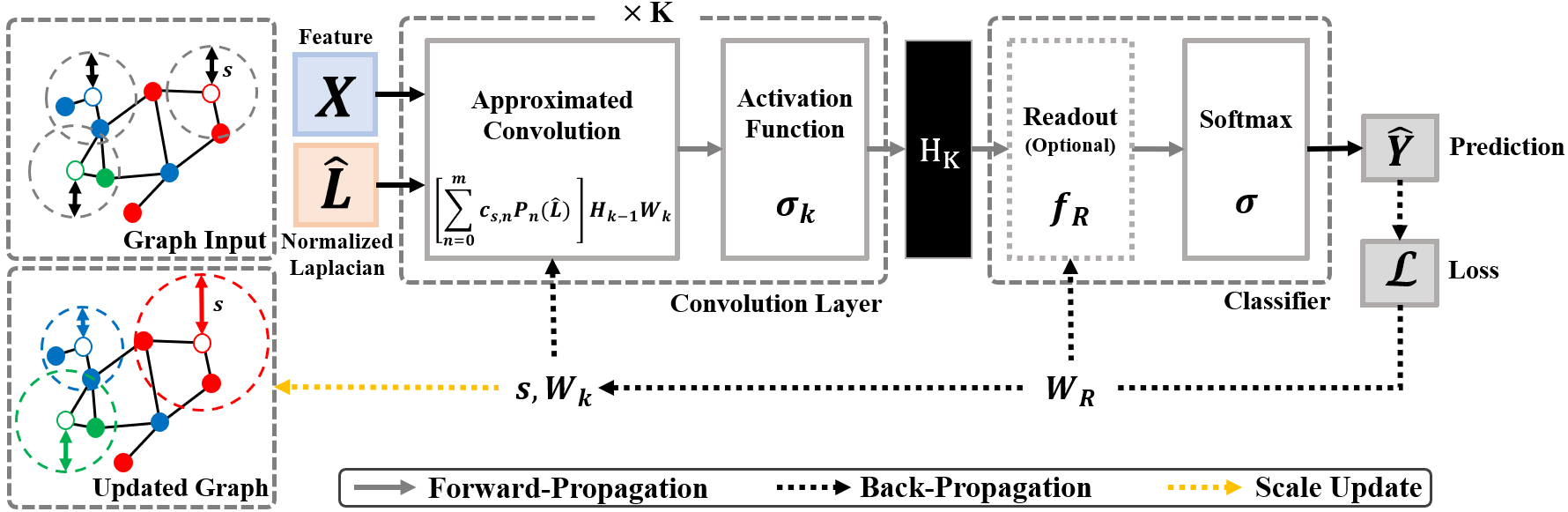
Figure 1: Illustration of LSAP. A graph (as normalized Laplacian $\hat{L}$) and node feature $X$ are inputted to the convolution layer. The output $H_{K}$ is inputted to a downstream classifier which yields a prediction $\hat{Y}$. The loss from $\hat{Y}$ is backpropagated to update the classifier and convolution approximation with $\textbf{s}=[s_{1},\dots,s_{N}]$ to adaptively adjust the scale of each node.

We introduce our model, i.e., LSAP, that trains on the approximations for the optimal range of neighborhood at individual nodes. The derivatives to train $s$ in Eq. (6) for two separate tasks, i.e., node classification and graph classification, are derived in their closed-forms.

Model Architecture

In most of GCN frameworks (Kipf et al. 2017; Yang et al. 2021), a convolution operation at the $k$-th layer is given as

$$H_{k}=\sigma_{k}(\tilde{A}H_{k-1}W_{k})$$ (7)

where $\tilde{A}$ is a normalized adjacency matrix, $W_{k}$ is a trainable weight matrix, and $\sigma_{k}$ is a non-linear activation function. It takes an input $H_{k-1}$ and outputs a new representation $H_{k}$. Each convolution operation takes features from direct neighbors of each node according to $\tilde{A}$ to design the new node representation. As more convolution layers are stacked, the range of aggregation is uniformly increased for all nodes causing the infamous “oversmoothing” issue. To alleviate oversmoothing, we propose to utilize a diffusion kernel, i.e., a heat kernel, on the graph to define ranges of neighborhood for individual nodes, so that the node-wise range is adaptively defined to avoid the oversmoothing.

The architecture of LSAP is given in Fig. 1. The overall components are similar to the original GCN (Kipf et al. 2017), however, LSAP redefines the convolution with approximated heat kernel. Consider a graph $G$ given as a Laplacian $\hat{L}$, feature $X$ defined on its nodes and either node-wise or graph-wise label $Y$. Our framework takes $\hat{L}$ and $X$ as inputs, performs approximated heat kernel convolutions and outputs a prediction $\hat{Y}$. The $\hat{Y}$ is then compared with the ground truth $Y$, and the error is backpropagated to update model parameters including the scale $s$.

Convolution Layer.

Based on Eq. (6), Eq. (7) is reformulated by replacing the normalized adjacency matrix $\tilde{A}$ with the heat kernel with polynomial approximation as

$$H_{k}=\sigma_{k}([\sum_{n=0}^{m}c_{s,n}P_{n}(\hat{L})]H_{k-1}W_{k}).$$ (8)

While $\tilde{A}$ let the model combine information from nodes within 1-hop distance only, Eq. (8) let it aggregate information within a “range” of each node defined by $s$ within $c_{s,n}$. The Eq. (8) defines a convolution layer, and we can stack $K$ of them to achieve a better representation of the original $X$.

Output Layer.

The output layer yields a prediction of $Y$, i.e., $\hat{Y}$, via softmax. Depending on the task, it may include a simple Multi-layer Perceptron (MLP) that can be trained. A loss $L_{\textbf{err}}$ is computed at this layer which quantifies the error between $\hat{Y}$ and $Y$ using cross-entropy for different tasks, e.g., node classification or graph classification.

Model Update.

The loss $L_{\textbf{err}}$ is backpropagated to update the model parameters, i.e., $W_{k}$ and $s$. To maintain the scale positive, an $\ell_{1}$-norm regularization on $s$ is imposed. The overall objective function $\mathcal{L}$ is given as

$$\mathcal{L}=\mathcal{L}_{\textbf{err}}+\alpha|{\bf s}|$$ (9)

where $\alpha$ is a hyperparameter. The weight $W_{k}$ can be easily trained with backpropagation, and a multi-variate s across all nodes can be also trained given a gradient on scale $s$ as

$$\textbf{s}\leftarrow\textbf{s}-\beta_{s}\frac{\partial\mathcal{L}}{\partial\textbf{s}}$$ (10)

where $\beta_{s}$ is a learning rate. It requires $\frac{\partial\mathcal{L}}{\partial\textbf{s}}$ to make the framework trainable, and we derive the $\frac{\partial\mathcal{L}}{\partial\textbf{s}}$ in a closed-form to train on the approximations of Eq. (8) in the following.

Gradients of Polynomial Coefficients with Scale

We denote expansion coefficients as $c_{\textbf{s},n}^{T}$, $c_{\textbf{s},n}^{H}$ and $c_{\textbf{s},n}^{L}$ that correspond to $P^{T}_{n}$, $P^{H}_{n}$ and $P^{L}_{n}$. As introduced in (Huang et al. 2020), one can obtain a solution to the heat diffusion by obtaining expansion coefficient with each polynomial in $P_{n}$. In order to design a gradient-based “learning” framework of node-wise range (i.e., scale) based on these expansions, we derived gradients of loss $\frac{\partial\mathcal{L}}{\partial\textbf{s}}$ in closed-forms. This is an essential component of LSAP as it let the model efficiently train without diagonalization of $\hat{L}$. The $\frac{\partial\mathcal{L}}{\partial\textbf{s}}$ can be achieved using the chain rule in a traditional way, and to obtain $\frac{\partial\mathcal{L}}{\partial\textbf{s}}$ in terms of the $H_{k}$, we compute $\frac{\partial c_{\textbf{s},n}}{\partial\textbf{s}}$ for each coefficient.

Chebyshev Polynomial.

The recurrence relation and expansion coefficient for Chebyshev polynomial are given as

$$P^{T}_{n+1}(\hat{L}) =(2-\delta_{n0})\hat{L}P^{T}_{n}(\hat{L})-P^{T}_{n-1}(\hat{L}),$$ (11)

$$c_{\textbf{s},n}^{T} =(2-\delta_{n0})(-1)^{n}e^{-\frac{\textbf{s}b}{2}}I_{n}\left(\frac{\textbf{s}b}{2}\right)$$

where $b>0$ is a hyper-parameter, and $I_{n}$ is the modified Bessel function of the first kind (Olver et al. 2010).

Hermite Polynomial.

The recurrence relation and expansion coefficient for Hermite polynomial are written as

$$P^{H}_{n+1}(\hat{L}) =2\hat{L}P^{H}_{n}(\hat{L})-2nP^{H}_{n-1}(\hat{L}),$$ (12)

$$c_{\textbf{s},n}^{H} =\frac{1}{n!}\left(\frac{-\textbf{s}}{2}\right)^{n}e^{\frac{\textbf{s}^{2}}{4}},$$

Laguerre Polynomial.

For Laguerre polynomial, the recurrence relation and expansion coefficient are

$$P^{L}_{n+1}(\hat{L}) =\frac{(2n+1-\hat{L})P^{L}_{n}(\hat{L})-nP^{L}_{n-1}(\hat{L})}{n+1},$$ (13)

$$c_{\textbf{s},n}^{L} =\frac{\textbf{s}^{n}}{(\textbf{s}+1)^{n+1}}.$$

Notice that all the expansion coefficients above are defined by s. If they are differentiable with respect to s, then we do not need to learn expensive parameters but simply train on these polynomial approximations with s directly.

Lemma 1.

Consider an orthogonal polynomial $P_{n}$ over interval $[a,b]$ with inner product $\int_{a}^{b}P_{n}(\lambda)P_{k}(\lambda)w(\lambda)d\lambda=\delta_{nk}$, where $w(\lambda)$ is the weight function. If $P_{n}$ expands the heat kernel, the expansion coefficients $c_{\textbf{s},n}$ with respect to s are differentiable and $\frac{\partial{c_{\textbf{s},n}}}{\partial{\textbf{s}}}=-\int_{a}^{b}\lambda e^{-\bf{s}\lambda}P_{n}(\lambda)w(\lambda)d\lambda$.

Lemma 1 (with a proof in the supplementary) says that the $c_{\textbf{s},n}$ in Eq. (11), (12) and (13) have the derivatives with respect to s. These will be used in the following two sections to define gradients on loss functions for different tasks.

Semi-supervised Node Classification

The goal of node classification is to predict labels of unlabeled nodes based on the information from other nodes. The output layer (after $K$-convolution layers) of LSAP produces a prediction $\hat{Y}=\sigma(H_{K})$, and the training should be performed to reduce the error between $\hat{Y}$ and the true $Y$.

Lemma 2.

Let a graph convolution be operated by Eq. (8), which approximates the convolution with $P_{n}$ and $c_{\textbf{s},n}$. If a loss $\mathcal{L}_{\textbf{err}}$ for node-wise classification is defined as cross-entropy between a prediction $\hat{Y}=\sigma(H_{K})$, where $\sigma(\cdot)$ is a softmax function, and the true $Y$, then

$$\frac{\partial\mathcal{L}_{\textbf{err}}}{\partial\textbf{s}}= (\hat{Y}-Y)\times\sigma^{{}^{\prime}}_{k}([\sum_{n=0}^{m}c_{\textbf{s},n}P_{n}(\hat{L})]H_{k-1}W_{k})W_{k}^{\mathsf{T}}$$ (14)

$$\times(\sum_{n=0}^{m}P_{n}(\hat{L})H_{k-1}^{\mathsf{T}}+[\sum_{n=0}^{m}c_{\textbf{s},n}P_{n}(\hat{L})]\frac{\partial H_{k-1}}{\partial c_{\textbf{s},n}})\frac{\partial c_{\textbf{s},n}}{\partial\textbf{s}}$$

where $\sigma^{{}^{\prime}}_{k}$ is the derivative of $\sigma_{k}$.

Lemma 2 let LSAP backpropagate the error to update s to obtain the optimal scale per node for node classification.

Graph Classification

Consider a population of graphs $\{G_{t}\}_{t=1}^{T}$ with corresponding labels $\{Y_{t}\}_{t=1}^{T}$, and learning a graph classification model finds a function $f(G_{t})=Y_{t}$. For this, the output layer consists of a readout layer $f_{R}(\cdot)$ (i.e., MLP with ReLU) and a softmax $\sigma(\cdot)$ at the end to construct pseudo-probability for each class. The $f_{R}(\cdot)$ with weights $W_{R}$ takes the output $H_{K}$ from the convolution layers as an input and returns $H_{R}$ as

$$H_{R}=f_{R}(H_{K};W_{R}),$$ (15)

and prediction $\hat{Y}=\sigma(H_{R})$.

Lemma 3.

Let $H_{k}$ from Eq. (8) be a graph convolution with a heat kernel with polynomial $P_{n}$ and coefficients $c_{\textbf{s},n}$. If a loss $\mathcal{L}_{\textbf{err}}$ for classifying graph-wise label is defined as cross-entropy between a prediction $\hat{Y}=\sigma(H_{R})$, where $\sigma(\cdot)$ is a softmax function, and the true $Y$, then

$$\frac{\partial\mathcal{L}_{\textbf{err}}}{\partial\textbf{s}}= (\hat{Y}-Y)\times\frac{\partial H_{R}}{\partial H_{K}}\times\sigma^{{}^{\prime}}_{k}([\sum_{n=0}^{m}c_{\textbf{s},n}P_{n}(\hat{L})]H_{k-1}W_{k})W_{k}^{\mathsf{T}}$$ (16)

$$\times(\sum_{n=0}^{m}P_{n}(\hat{L})H_{k-1}^{\mathsf{T}}+[\sum_{n=0}^{m}c_{\textbf{s},n}P_{n}(\hat{L})]\frac{\partial H_{k-1}}{\partial c_{\textbf{s},n}})\frac{\partial c_{\textbf{s},n}}{\partial\textbf{s}}$$

where $\sigma^{{}^{\prime}}_{k}$ is the derivative of $\sigma_{k}$.

Lemma 3 let LSAP adaptively update the scale s across all nodes for each node using Eq. (10) towards the minimal error for predicting graph-wise label.

Experiments

In this section, we compare the performances of LSAP and baselines on node classification and graph classification. LSAP-C, LSAP-H and LSAP-L correspond to approximation frameworks with $P^{T}_{n}$, $P^{H}_{n}$ and $P^{L}_{n}$, and the model with exact computation of the heat kernel convolution is referred as Exact. For the node classification, we used conventional benchmarks for semi-supervised learning task (Shchur et al. 2018). For the graph classification, we investigated real brain network data from Alzheimer’s Disease Neuroimaging Initiative (ADNI) to classify different diagnostic stages towards Alzheimer’s Disease (AD) for a practical application. These tasks on seven different benchmarks can demonstrate the feasibility of LSAP.

Semi-supervised Node Classification

Datasets.

We conducted experiments on standard node classification datasets (in Table 1) that provide connected and undirected graphs. Cora, Citeseer and Pubmed (Sen et al. 2008) are constructed as citation networks, Amazon Computer and Amazon Photo (Shchur et al. 2018) define co-purchase networks, and Coauthor CS (Shchur et al. 2018) is a co-authorship network.

Dataset	Nodes	Edges	Classes	Features
Cora	2,708	5,429	7	1,433
Citeseer	3,327	4,732	6	3,703
Pubmed	19,717	44,338	3	500
Amazon Computers	13,752	245,861	10	767
Amazon Photo	7,650	119,081	8	745
Coauthor CS	18,333	81,894	15	6,805

Table 1: Summary of node classification datasets.

Setup.

We used the accuracy as the evaluation metric. For Cora, Citseer and Pubmed data, eighteen different baselines were used to compare the results for the node classification task as listed in Table 2. These standard benchmarks are provided with fixed split of 20 nodes per class for training, 500 nodes for validation and 1000 nodes for testing as in other literature (Kim et al. 2022; Wu et al. 2022b).

For Amazon and Coauthor datasets, seven baselines are used as in Table 3. For the MLP with 3-layers, GCN and 3ference, results are obtained from (Luo et al. 2022), and a result for DSF comes from (Guo et al. 2023). For others, the experiments were performed by randomly splitting the data as 60%/20%/20% for training/validation/testing datasets as in (Luo et al. 2022) and replicating it 10 times to obtain mean and standard deviation of the evaluation metric.

Model	Cora	Citeseer	Pubmed
GCN (Kipf et al. 2017)	81.50	70.30	78.60
GAT (Veličković et al. 2018)	83.00	72.50	79.00
APPNP (Klicpera et al. 2019b)	83.30	71.80	80.10
$\text{GDC}^{{\dagger}}$ (Klicpera et al. 2019a)	82.20	71.80	79.10
SGC (Wu et al. 2019)	81.70	71.30	78.90
Bayesian GCN (Zhang et al. 2019a)	81.20	72.20	-
Shoestring (Lin, Gao, and Li 2020)	81.90	69.50	79.70
$\text{GraphHeat}^{{\dagger}}$ (Xu et al. 2020)	83.70	72.50	80.50
g-U-Nets (Gao et al. 2019)	84.40	73.20	79.60
GCNII (Chen et al. 2020)	85.50	73.40	80.30
GRAND (Feng et al. 2020)	85.40	75.40	82.70
DAGNN (Liu et al. 2020)	84.40	73.30	80.50
SelfSAGCN (Yang et al. 2021)	83.80	73.50	80.70
DIAL-GNN (Chen et al. 2021)	84.50	74.10	-
SuperGAT (Kim et al. 2022)	84.30	72.60	81.70
$\text{GRAND}^{{\dagger}}$ (Chamberlain et al. 2021)	83.60	74.10	78.80
$\text{ADC}^{{\dagger}}$ (Zhao et al. 2021)	84.50	74.50	83.00
SEP-N (Wu et al. 2022b)	84.80	72.90	80.20
LSAP-C	87.90	76.50	83.30
LSAP-H	85.00	76.10	82.60
LSAP-L	85.90	75.90	84.10
Exact	88.20	78.10	85.30

${\dagger}$: graph diffusion-based models.

Table 2: Accuracy (%) on Cora, Citeseer, and Pubmed. LSAP yields better performances over existing baselines (in bold) similar to Exact achieving the best results (underline).

Model	Amazon	Amazon	Coauthor
	Computer	Photo	CS
MLP (3-layers)	84.63	91.96	95.63
GCN	90.49	93.91	93.32
3ference	90.74	95.05	95.99
GAT	91.18 $\pm$ 0.74	94.49 $\pm$ 0.54	93.42 $\pm$ 0.31
GDC	86.03 $\pm$ 2.26	93.28 $\pm$ 1.03	92.68 $\pm$ 0.53
GraphHeat	89.59 $\pm$ 3.15	94.04 $\pm$ 0.75	92.93 $\pm$ 0.20
DSF	92.84 $\pm$ 0.10	95.73 $\pm$ 0.08	-
LSAP-C	94.43 $\pm$ 1.16	95.96 $\pm$ 1.65	94.81 $\pm$ 0.55
LSAP-H	93.64 $\pm$ 0.86	96.65 $\pm$ 0.67	93.52 $\pm$ 0.97
LSAP-L	92.76 $\pm$ 0.48	95.35 $\pm$ 0.85	93.58 $\pm$ 0.82
Exact	93.52 $\pm$ 0.65	96.41 $\pm$ 1.54	93.71 $\pm$ 1.16

Table 3: Mean node classification accuracy (%) and s.d. on Amazon Computers, Amazon Photo, and Coauthor CS. The best results are in bold, and the best results within experiments with replicates are underlined.

Results.

Table 2 and 3 show the performance comparisons between LSAP and baseline models. As shown in Table 2, on the node classification benchmarks, learning node-wise adaptive scale performs the best in both Exact and its approximations. LSAP showed improved performance over existing models; exceeding previous best baseline performances by 2.4% (on Cora) and 1.1% (on Citeseer and Pubmed) The similar performance of LSAP with that of Exact demonstrates accurate convolution approximation. Despite slight decreases, training on adaptive scales using LSAP was much faster.

For additional datasets in Table 3, the performance of LSAP outperformed the baselines. The results for MLP, GCN and 3ference were adopted from (Luo et al. 2022), which reported the best performance out of 10 replicated experiments. We ran the same experiments for GAT, GDC, GraphHeat, Exact and LSAP, and the mean and standard deviation of metrics are given. LSAP shows significant improvements on the Amazon Computer (94.43%, LSAP-C) and Amazon Photo (96.65%, LSAP-H). On the Coauther CS, we also achieve the highest mean accuracy (94.81%, LSAP-C) among the experiments with random replicates.

Biomarker	Category	CN	SMC	EMCI	LMCI	AD
Cortical Thickness	# of subjects	359	181	437	180	166
	Gender (M / F)	178 / 181	69 / 112	249 / 188	119 / 61	102 / 64
	Age (Mean$\pm$Std)	72.8$\pm$1.4	72.0$\pm$5.2	71.0$\pm$7.9	70.9$\pm$6.1	74.8$\pm$8.7
FDG	# of subjects	345	186	461	231	162
	Gender (M / F)	173 / 172	66 / 120	262 / 199	152 / 79	102 / 60
	Age (Mean$\pm$Std)	73.0$\pm$1.3	71.7$\pm$5.2	71.7$\pm$7.8	71.1$\pm$7.0	74.9$\pm$8.8

Table 4: Demographics of the ADNI dataset.

Graph Classification

Datasets.

Using the magnetic resonance images (MRI) from the ADNI data, each brain was partitioned into 148 cortical regions and 12 sub-cortical regions using Destrieux atlas (Destrieux et al. 2010), and tractography on diffusion-weighted imaging (DWI) was applied to calculate the number of white matter fibers connecting the 160 brain regions to construct $160\times 160$ structural network (i.e., graph). On the same parcellation, region-wise imaging features such as Standard Uptake Value Ratio (SUVR) of metabolism level from FDG-PET and cortical thickness from MRI were measured. For the SUVR normalization, Cerebellum was used as the reference. The dataset consists of 5 AD-specific progressive groups: Control (CN), Significant Memory Concern (SMC), Early Mild Cognitive Impairment (EMCI), Late Mild Cognitive Impairment (LMCI) and AD. The demographics of ADNI dataset are summarized in Table 4.

Feature	Model	Classification (ADNI)
		Accuracy (%)	Precision	Recall
Cortical Thickness	SVM (Linear)	82.39 $\pm$ 2.73	0.822 $\pm$ 0.033	0.852 $\pm$ 0.025
	MLP (2-layers)	78.76 $\pm$ 2.21	0.792 $\pm$ 0.036	0.799 $\pm$ 0.026
	GCN	61.37 $\pm$ 3.09	0.598 $\pm$ 0.025	0.626 $\pm$ 0.044
	GAT	64.17 $\pm$ 5.46	0.627 $\pm$ 0.067	0.668 $\pm$ 0.046
	GDC	77.10 $\pm$ 4.25	0.769 $\pm$ 0.050	0.785 $\pm$ 0.044
	GraphHeat	70.90 $\pm$ 3.17	0.703 $\pm$ 0.030	0.718 $\pm$ 0.026
	ADC	82.10 $\pm$ 2.41	0.776 $\pm$ 0.019	0.728 $\pm$ 0.067
	LSAP-C	87.00 $\pm$ 2.16	0.868 $\pm$ 0.027	0.885 $\pm$ 0.027
	LSAP-H	85.41 $\pm$ 2.32	0.859 $\pm$ 0.031	0.867 $\pm$ 0.030
	LSAP-L	85.64 $\pm$ 1.86	0.859 $\pm$ 0.022	0.866 $\pm$ 0.022
	Exact	86.24 $\pm$ 1.96	0.866 $\pm$ 0.017	0.867 $\pm$ 0.023
FDG	SVM (Linear)	85.27 $\pm$ 2.09	0.857 $\pm$ 0.027	0.869 $\pm$ 0.021
	MLP (2-layers)	87.51 $\pm$ 1.62	0.882 $\pm$ 0.024	0.882 $\pm$ 0.014
	GCN	68.81 $\pm$ 1.95	0.677 $\pm$ 0.028	0.697 $\pm$ 0.025
	GAT	69.24 $\pm$ 7.13	0.670 $\pm$ 0.106	0.736 $\pm$ 0.037
	GDC	86.21 $\pm$ 3.24	0.867 $\pm$ 0.033	0.870 $\pm$ 0.029
	GraphHeat	76.97 $\pm$ 2.42	0.775 $\pm$ 0.035	0.773 $\pm$ 0.010
	ADC	88.60 $\pm$ 2.81	0.708 $\pm$ 0.062	0.753 $\pm$ 0.053
	LSAP-C	89.24 $\pm$ 2.23	0.895 $\pm$ 0.022	0.904 $\pm$ 0.023
	LSAP-H	90.11 $\pm$ 2.44	0.903 $\pm$ 0.027	0.910 $\pm$ 0.022
	LSAP-L	90.40 $\pm$ 1.38	0.909 $\pm$ 0.018	0.914 $\pm$ 0.015
	Exact	90.18 $\pm$ 2.67	0.907 $\pm$ 0.028	0.907 $\pm$ 0.028

Table 5: Classification performances on ADNI dataset.

Setup.

5-way classification was designed to classify the different groups in Table 4. 5-fold cross validation was used to obtain unbiased results, and accuracy, precision, and recall in their mean were used as evaluation metrics. As the baseline, we adopted Linear Support Vector Machine (SVM), Multi-Layer Perceptron (MLP) with 2 layers, GCN (Kipf et al. 2017), GAT (Veličković et al. 2018), GDC (Klicpera et al. 2019a), GraphHeat (Xu et al. 2020) and ADC (Zhao et al. 2021). Each sample is given with a graph (i.e., brain network) and two node features (i.e., cortical thickness and FDG measure) which are well-known as useful biomarkers for AD diagnosis.

Cora	Citeseer
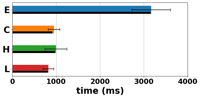
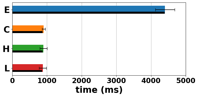
Pubmed	ADNI

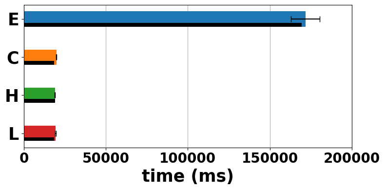
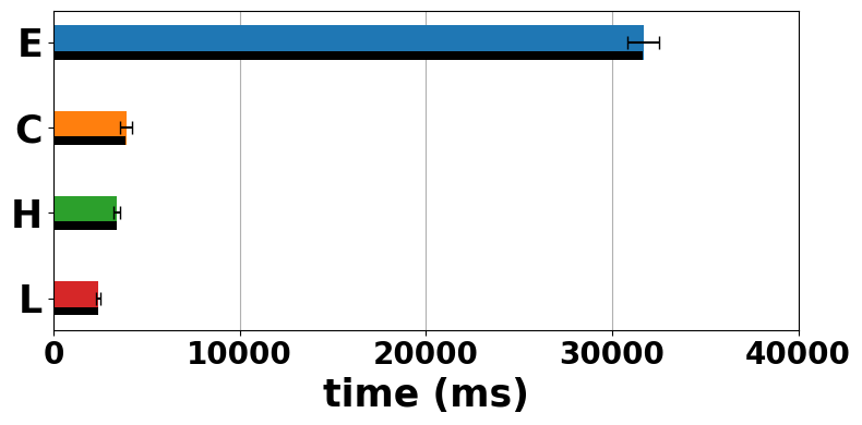
Figure 2: Comparisons of computation time (in ms) for one epoch (Forward and backpropagation). Within the epoch, time for heat kernel convolution is given in black bar. Results were obtained with 10 repetitions.

Exact	LSAP-C	LSAP-H	LSAP-L

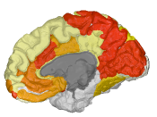
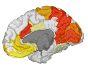
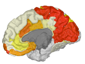
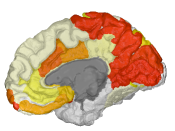
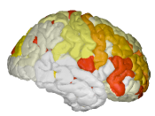
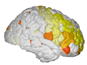
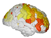
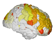
Figure 3: Visualization of the learned scales on the cortical regions of a brain. This visualization shows the scale of each ROI from the classification result using FDG feature. Top: Inner part of right hemisphere, Bottom: Outer part of right hemisphere.

Results.

The performances including accuracy, precision, and recall between LSAP and seven baselines on the ADNI dataset are shown in Table 5. LSAP showed accuracy $\sim$86% using cortical thickness and $\sim$90% with FDG in classifying the 5 diagnostic stages of AD, with precision and recall $\sim$0.86 and 0.91, respectively. These numbers are approximately the same with the results from Exact and low standard deviations from LSAP demonstrate feasibility of the approximation. LSAP performed the best surpassing the second best methods by 4.61%p and 1.80%p in accuracy for cortical thickness and FDG experiments, respectively.

Model Behavior Analysis

Computation Time with Kernel Convolution.

Fig. 2 compares averaged empirical time (in ms) spent for one epoch of training process of Exact and LSAP on node classification task (on Cora, Citesser and Pubmed) and graph classification task (on ADNI) with 10 replicates. The colors denote the type of methods, and as seen in Fig. 2, LSAP takes far less time than Exact computation. Notice that the computation of kernel convolution takes the majority of time (in black bar), and the approximations make this process efficient. For the node classification, approximation on Pubmed showed the best efficiency as its graph had the largest number of nodes (19717) compared to Cora (2708) and Citeseer (3327). For the graph classification, approximations were even more efficient as eigendecomposition of $\hat{L}$ from all subjects had to be performed for Exact. Comparing the computation time of a single epoch on Exact and LSAP-L, the time is saved by $\sim$93%.

ROI (Destrieux et al. 2010)	Exact	LSAP-C	LSAP-H	LSAP-L
(L) G&S.paracentral	0.034	0.052	0.049	0.066
(L) G.front.inf.Orbital	0.036	0.071	0.060	0.043
(R) G.precuneus	0.041	0.044	0.034	0.051
(R) S.ortibal.med.olfact	0.047	0.078	0.054	0.059
(R) G.cingul.Post.ventral	0.055	0.056	0.055	0.051
(R) S.oc.temp.lat	0.055	0.065	0.045	0.063
(R) G.oc.temp.med.Lingual	0.055	0.076	0.043	0.040
(L) Sub.put	0.058	0.077	0.047	0.060
(L) S.postcentral	0.061	0.069	0.060	0.018
(R) G.front.inf.Orbital	0.063	0.093	0.069	0.050

Table 6: 10 ROIs with the smallest trained scales for AD classification. (L)/(R) denote the left/right hemisphere.

Discussions on the Scales for Graph Classification.

In AD classification, we performed graph classification to distinguish the different diagnostic labels of AD. The trained model yields node-wise optimized scale where the node corresponds to specific region of interest (ROI) in the brain. The trained scales denote the optimal ranges of neighborhood for each ROI. Therefore, if the trained scale is small for a specific node, it means that the node does not have to look far to contribute to the classification. On the other hand, the nodes with large scales need to aggregate information from far distances to constitute an effective embedding as it is not very useful on its own. The trained scales on the brain network classification with Exact and LSAP are visualized in Fig. 3 conveying two important perspectives. First, the scales delineate which of the ROIs are independently behaving to classify AD-specific labels. Second, the trained scales with LSAP are quite similar to the result from Exact meaning that the approximation is feasibly accurate for practical uses.

In Table 6, 10 ROIs with the smallest scales that appear in common across Exact and LSAPs are listed. Inferior frontal orbital gyrus on both hemispheres is captured, and several temporal/orbital regions, precuneous, and left putamen are shown to yield small scales. These ROIs are known as highly AD-specific by various literature (Galton et al. 2001; Bailly et al. 2015; de Jong et al. 2008; Hoesen et al. 2000).

Effect of $K$.

We examined the performance of LSAP with respect to the number of convolution layers $K$ on Cora and ADNI experiments. When $K$ was varied from 1 to 4 under the same setting, $K$=2 showed the best performance in both experiments. The performance decreases when $K$=3 and 4 may be due to lack of training samples as the model sizes are drastically increased. We observed the same pattern across Exact and LSAP, which demonstrates LSAP with approximation is able to train on the scales properly.

Cora	ADNI

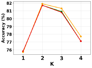
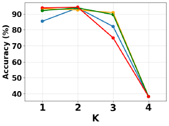
Figure 4: Effect of the number of layers $K$ on model performance. Left: accuracy of node classification on Cora, Right: accuracy of graph classification on ADNI.

Conclusions

In this work, we proposed efficient trainable methods to bypass exact computation of spectral kernel convolution that define adaptive ranges of neighbor for each node. We have derived closed-form derivatives on polynomial coefficients to train the scale with conventional backpropagation, and the developed framework LSAP demonstrates SOTA performance on node classification and brain network classification. The brain network analysis provides neuroscientifically interpretable results corroborated by previous AD literature.

Summary

This material presents the supplementary paper from the main paper due to the space limitation. In Section 1, the detailed calculation process of gradient for coefficients are presented. In Section 2, the proofs of each Lemma from the main paper are provided. Additional details for LSAP architecture that were omitted from the main manuscript are presented in Section 3. In Section 4, hyperparameters of LSAP and baselines for both node classification and graph classification and more results on brain network classification on ADNI data are shown. The implementation details are written in Section 5, and detailed model complexity is in Section 6. Adjustment of the trained scales at training phase is visualized in Section 7. Finally, we additionally discuss our framework in Section 8.

1. Gradients of Polynomial Coefficients with Scale

In this section, we are going to show the detailed derivation of gradient $\frac{\partial c_{s,n}}{\partial s}$ for the three polynomials, i.e., Chebyshev, Hermite and Laguerre.

Chebyshev Polynomial. The expansion coefficient for Chebyshev polynomial is given as

$$c_{s,n}^{T} =(2-\delta_{n0})(-1)^{n}e^{-\frac{sb}{2}}I_{n}\left(\frac{sb}{2}\right),$$ (17)

and the derivative of $c_{s,n}^{T}$ with respect to $s$ is obtained as

$$\frac{\partial c_{s,n}^{T}}{\partial s} =2(-1)^{n}e^{\frac{-sb}{2}}\left(\frac{-b}{2}\right)I_{n}\left(\frac{sb}{2}\right)$$ (18)

$$\quad+2(-1)^{n}e^{\frac{-sb}{2}}I_{n}\left(\frac{sb}{2}\right)\frac{b}{2}$$

$$=2(-1)^{n}e^{\frac{-sb}{2}}\left(-\frac{b}{2}I_{n}\left(\frac{sb}{2}\right)+\frac{b}{2}I_{n}^{{}^{\prime}}\left(\frac{sb}{2}\right)\right)$$

$$=(-1)^{n}be^{\frac{-sb}{2}}\left(I_{n}^{{}^{\prime}}\left(\frac{sb}{2}\right)-I_{n}\left(\frac{sb}{2}\right)\right)$$

$$=(-1)^{n}be^{\frac{-sb}{2}}\left(I_{n-1}\left(\frac{sb}{2}\right)-\frac{n}{\frac{sb}{2}}I_{n}\left(\frac{sb}{2}\right)-I_{n}\left(\frac{sb}{2}\right)\right)$$

$$=(-1)^{n}be^{\frac{-sb}{2}}\left(I_{n-1}\left(\frac{sb}{2}\right)-\left(\frac{2n}{sb}+1\right)I_{n}\left(\frac{sb}{2}\right)\right)$$

$$\left(\because I_{n}^{{}^{\prime}}(x)=I_{n-1}(x)-\frac{n}{x}I_{n}(x)\right).$$

Hermite Polynomial. The expansion coefficient for Hermite polynomial is written as

$$c_{s,n}^{H} =\frac{1}{n!}\left(\frac{-s}{2}\right)^{n}e^{\frac{s^{2}}{4}},$$ (19)

and the derivative of $c_{s,n}^{H}$ with respect to $s$ is computed as

$$\frac{\partial c_{s,n}^{H}}{\partial s} =\frac{n}{n!}\left(\frac{-s}{2}\right)^{n-1}\left(\frac{-1}{2}\right)e^{\frac{s^{2}}{4}}+\frac{1}{n!}\left(\frac{-s}{2}\right)^{n}e^{\frac{s^{2}}{4}}\frac{s}{2}$$ (20)

$$=\frac{1}{n!}e^{\frac{s^{2}}{4}}\left(\frac{-s}{2}\right)^{n}\left(\frac{-n}{2}\left(\frac{-s}{2}\right)^{-1}+\frac{s}{2}\right)$$

$$=\frac{1}{n!}e^{\frac{s^{2}}{4}}\left(\frac{-s}{2}\right)^{n}\left(\frac{n}{s}+\frac{s}{2}\right)$$

$$=\frac{1}{n!}e^{\frac{s^{2}}{4}}\left(\frac{-s}{2}\right)^{n}\frac{n}{s}\frac{s}{2}\frac{2}{s}+\frac{1}{n!}e^{\frac{s^{2}}{4}}\left(\frac{-s}{2}\right)^{n}\frac{s}{2}$$

$$=\frac{se^{\frac{s^{2}}{4}}}{2n!}\left(\frac{-s}{2}\right)^{n}\left(\frac{2n}{s^{2}}+1\right).$$

Laguerre Polynomial. The expansion coefficient for Laguerre polynomial is written as

$$c_{s,n}^{L} =\frac{s^{n}}{(s+1)^{n+1}},$$ (21)

and the derivative of $c_{s,n}^{L}$ with respect to $s$ is calculated as

$$\frac{\partial c_{s,n}^{L}}{\partial s} =\frac{ns^{n-1}\left(s+1\right)^{n+1}-s^{n}\left(n+1\right)\left(s+1\right)^{n}}{\left\{\left(s+1\right)^{n+1}\right\}^{2}}$$ (22)

$$=\frac{ns^{n-1}\left(s+1\right)^{n+1}-s^{n}\left(n+1\right)\left(s+1\right)^{n}}{\left(s+1\right)^{2n}\left(s+1\right)^{2}}$$

$$=\frac{ns^{n-1}\left(s+1\right)-s^{n}\left(n+1\right)}{\left(s+1\right)^{n}\left(s+1\right)^{2}}$$

$$=\frac{ns^{n}+ns^{n-1}-ns^{n}-s^{n}}{\left(s+1\right)^{n+2}}$$

$$=\frac{ns^{n-1}-s^{n}}{\left(s+1\right)^{n+2}}$$

$$=\frac{\left(\frac{n}{s}-1\right)s^{n}}{\left(s+1\right)^{n+2}}$$

$$=\frac{s^{n-1}(n-s)}{(s+1)^{n+2}}.$$

2. Proofs of Lemma

Lemma 1.

Consider an orthogonal polynomial $P_{n}$ over interval $[a,b]$ with inner product $\int_{a}^{b}P_{n}(\lambda)P_{k}(\lambda)w(\lambda)d\lambda=\delta_{nk}$, where $w(\lambda)$ is the weight function. If $P_{n}$ expands the heat kernel, the expansion coefficients $c_{\textbf{s},n}$ with respect to s are differentiable and $\frac{\partial{c_{\textbf{s},n}}}{\partial{\textbf{s}}}=-\int_{a}^{b}\lambda e^{-\bf{s}\lambda}P_{n}(\lambda)w(\lambda)d\lambda$.

Proof.

From (Huang et al. 2020) and Eq. (4) in the main paper, the exponential weight of the heat kernel can be expanded by polynomials $P_{n}$ and coefficients $c_{\textbf{s},n}$ as

$$e^{-\textbf{s}\lambda}=\sum_{n=0}^{\infty}c_{\textbf{s},n}P_{n}(\lambda).$$ (23)

Multiplying both sides of Eq. (23) by $P_{k}(\lambda)w(\lambda)$, and taking the integral over $\lambda$ from a to b,

$$\int_{a}^{b}e^{-\textbf{s}\lambda}P_{k}(\lambda)w(\lambda)d\lambda=\int_{a}^{b}\sum_{n=0}^{\infty}c_{\textbf{s},n}P_{n}(\lambda)P_{k}(\lambda)w(\lambda)d\lambda.$$ (24)

Since $P_{n}$ is an orthogonal polynomial and satisfies the inner product equation, $\int_{a}^{b}P_{n}(\lambda)P_{k}(\lambda)w(\lambda)d\lambda=\delta_{nk}$, so the right-hand side of Eq. (24) follows as

$$\int_{a}^{b}\sum_{n=0}^{\infty}c_{\textbf{s},n}P_{n}(\lambda)P_{k}(\lambda)w(\lambda)d\lambda$$ (25)

$$=\sum_{n=0}^{\infty}c_{\textbf{s},n}\int_{a}^{b}P_{n}(\lambda)P_{k}(\lambda)w(\lambda)d\lambda$$

$$=\sum_{n=0}^{\infty}c_{\textbf{s},n}\delta_{nk}.$$

$\delta_{nk}$ in Eq. (25) is equal to one when $n=k$, otherwise zero. So, $c_{\textbf{s},n}$ can be expressed as

$$c_{\textbf{s},n}=\int_{a}^{b}e^{-\textbf{s}\lambda}P_{n}(\lambda)w(\lambda)d\lambda.$$ (26)

From the Eq. (26), the s only depends on the exponential term, $e^{-\textbf{s}\lambda}$. Therefore, the expansion coefficients of the heat kernel are differentiable, and the derivative is

$$\frac{\partial{c_{\textbf{s},n}}}{\partial{\textbf{s}}}=-\int_{a}^{b}\lambda e^{-\bf{s}\lambda}P_{n}(\lambda)w(\lambda)d\lambda.$$ (27)

∎

Lemma 2.

Let a graph convolution be operated by Eq. (8) (in the main paper), which approximates the convolution with $P_{n}$ and $c_{\textbf{s},n}$. If a loss $\mathcal{L}_{\textbf{err}}$ for node-wise classification is defined as cross-entropy between a prediction $\hat{Y}=\sigma(H_{K})$, where $\sigma(\cdot)$ is a softmax function, and the true $Y$, then

$$\frac{\partial\mathcal{L}_{\textbf{err}}}{\partial\textbf{s}}= (\hat{Y}-Y)\times\sigma^{{}^{\prime}}_{k}([\sum_{n=0}^{m}c_{\textbf{s},n}P_{n}(\hat{L})]H_{k-1}W_{k})W_{k}^{\mathsf{T}}$$ (28)

$$\times(\sum_{n=0}^{m}P_{n}(\hat{L})H_{k-1}^{\mathsf{T}}+[\sum_{n=0}^{m}c_{\textbf{s},n}P_{n}(\hat{L})]\frac{\partial H_{k-1}}{\partial c_{\textbf{s},n}})\frac{\partial c_{\textbf{s},n}}{\partial\textbf{s}}$$

where $\sigma^{{}^{\prime}}_{k}$ is the derivative of $\sigma_{k}$.

Proof.

Let $N$ be the number of nodes, and $J$ be the number of labels. The loss $\mathcal{L}_{\textbf{err}}$ across all labeled nodes $V^{L}$ is defined as

$$\mathcal{L}_{\textbf{err}}=-\frac{1}{N}\sum_{i\in V^{L}}\sum_{j=1}^{J}Y_{ij}\text{ln}\hat{Y}_{ij}.$$ (29)

The derivative of $\mathcal{L}$ can be calculated with respect to scale s of $c_{\textbf{s},n}$ via chain rule as,

$$\frac{\partial\mathcal{L}_{\textbf{err}}}{\partial\textbf{s}}=\frac{\partial\mathcal{L}_{\textbf{err}}}{\partial H_{K}}\frac{\partial H_{K}}{\partial c_{\textbf{s},n}}\frac{\partial c_{\textbf{s},n}}{\partial\textbf{s}}.$$ (30)

Since we use softmax to produce pseudo-probability, the $\frac{\partial\mathcal{L}_{\textbf{err}}}{\partial H_{K}}$ is derived as

$$\frac{\partial\mathcal{L}_{\textbf{err}}}{\partial H_{K}}=\hat{Y}-Y.$$ (31)

From Eq. (8) in the main paper, the $\frac{\partial H_{K}}{\partial c_{\textbf{s},n}}$ becomes

$$\frac{\partial H_{K}}{\partial c_{\textbf{s},n}} =\sigma^{{}^{\prime}}_{k}([\sum_{n=0}^{m}c_{\textbf{s},n}P_{n}(\hat{L})]H_{k-1}W_{k})\times W_{k}^{\mathsf{T}}$$ (32)

$$\times(\sum_{n=0}^{m}P_{n}(\hat{L})H_{k-1}^{\mathsf{T}}+[\sum_{n=0}^{m}c_{\textbf{s},n}P_{n}(\hat{L})]\frac{\partial H_{k-1}}{\partial c_{\textbf{s},n}})$$

where the derivative of $H_{k}$ is recursively defined with $H_{k-1}$ along the hidden layer. Using chain rule with Eq. (31), (32) and $\frac{\partial c_{\textbf{s},n}}{\partial\textbf{s}}$ that depends on the type of polynomial, the gradient on $\mathcal{L}_{\textbf{err}}$ for node classification is written as

$$\frac{\partial\mathcal{L}_{\textbf{err}}}{\partial\textbf{s}}= (\hat{Y}-Y)\times\sigma^{{}^{\prime}}_{k}([\sum_{n=0}^{m}c_{\textbf{s},n}P_{n}(\hat{L})]H_{k-1}W_{k})W_{k}^{\mathsf{T}}$$ (33)

$$\times(\sum_{n=0}^{m}P_{n}(\hat{L})H_{k-1}^{\mathsf{T}}+[\sum_{n=0}^{m}c_{\textbf{s},n}P_{n}(\hat{L})]\frac{\partial H_{k-1}}{\partial c_{\textbf{s},n}})\frac{\partial c_{\textbf{s},n}}{\partial\textbf{s}}.$$

∎

Lemma 3.

Let $H_{k}$ from Eq. (8) (in the main paper) be a graph convolution operation, which is operated by the heat kernel with polynomial $P_{n}$ and coefficients $c_{\textbf{s},n}$. If a loss $\mathcal{L}_{\textbf{err}}$ for classifying graph-wise label is defined as cross-entropy between a prediction $\hat{Y}=\sigma(H_{R})$, where $\sigma(\cdot)$ is a softmax function, and the true $Y$, then

$$\frac{\partial\mathcal{L}_{\textbf{err}}}{\partial\textbf{s}}= (\hat{Y}-Y)\times\frac{\partial H_{R}}{\partial H_{K}}\times\sigma^{{}^{\prime}}_{k}([\sum_{n=0}^{m}c_{\textbf{s},n}P_{n}(\hat{L})]H_{k-1}W_{k})W_{k}^{\mathsf{T}}$$ (34)

$$\times(\sum_{n=0}^{m}P_{n}(\hat{L})H_{k-1}^{\mathsf{T}}+[\sum_{n=0}^{m}c_{\textbf{s},n}P_{n}(\hat{L})]\frac{\partial H_{k-1}}{\partial c_{\textbf{s},n}})\frac{\partial c_{\textbf{s},n}}{\partial\textbf{s}}$$

where $\sigma^{{}^{\prime}}_{k}$ is the derivative of $\sigma_{k}$.

Proof.

Let $T$ be the sample size, and $J$ be the set of class labels. As in the node classification, the loss $\mathcal{L}_{\textbf{err}}$ is defined with cross-entropy as

$$\mathcal{L}_{\textbf{err}}=-\frac{1}{T}\sum_{t=1}^{T}\sum_{j\in J}Y_{tj}\text{ln}\hat{Y}_{tj}$$ (35)

Also, the derivative of $\mathcal{L}$ can be calculated in terms of scale $s$ of $c_{s,n}$ via chain rule. As we use an additional MLP for graph classification, i.e., Eq. (15) in the main paper, the gradient of $\mathcal{L}_{\textbf{err}}$ along $H_{R}$ must be computed and plugged into Eq. (28) as

$$\frac{\partial\mathcal{L}_{\textbf{err}}}{\partial\textbf{s}}=\frac{\partial\mathcal{L}_{\textbf{err}}}{\partial H_{R}}\frac{\partial H_{R}}{\partial H_{K}}\frac{\partial H_{K}}{\partial c_{\textbf{s},n}}\frac{\partial c_{\textbf{s},n}}{\partial\textbf{s}}.$$ (36)

Since the activation function of output layer is a softmax, the $\frac{\partial\mathcal{L}_{\textbf{err}}}{\partial H_{R}}$ are the same as Eq.  (31),

$$\frac{\partial\mathcal{L}_{\textbf{err}}}{\partial H_{R}}=\hat{Y}-Y.$$ (37)

The $\frac{\partial H_{R}}{\partial H_{k}}$ varies depending on the choice of $H_{R}$, and the $\frac{\partial H_{k}}{\partial c_{\textbf{s},n}}$ is the same as Eq. (32),

$$\frac{\partial H_{K}}{\partial c_{\textbf{s},n}} =\sigma^{{}^{\prime}}_{k}([\sum_{n=0}^{m}c_{\textbf{s},n}P_{n}(\hat{L})]H_{k-1}W_{k})\times W_{k}^{\mathsf{T}}$$ (38)

$$\times(\sum_{n=0}^{m}P_{n}(\hat{L})H_{k-1}^{\mathsf{T}}+[\sum_{n=0}^{m}c_{\textbf{s},n}P_{n}(\hat{L})]\frac{\partial H_{k-1}}{\partial c_{\textbf{s},n}}).$$

With these components and $\frac{\partial c_{\textbf{s},n}}{\partial\textbf{s}}$ that depends on the type of polynomial, the gradient on $\mathcal{L}_{\textbf{err}}$ is computed as

$$\frac{\partial\mathcal{L}_{\textbf{err}}}{\partial\textbf{s}} =(\hat{Y}-Y)\times\frac{\partial H_{R}}{\partial H_{K}}\times\sigma^{{}^{\prime}}_{k}([\sum_{n=0}^{m}c_{\textbf{s},n}P_{n}(\hat{L})]H_{k-1}W_{k})W_{k}^{\mathsf{T}}$$ (39)

$$\times(\sum_{n=0}^{m}P_{n}(\hat{L})H_{k-1}^{\mathsf{T}}+[\sum_{n=0}^{m}c_{\textbf{s},n}P_{n}(\hat{L})]\frac{\partial H_{k-1}}{\partial c_{\textbf{s},n}})\frac{\partial c_{\textbf{s},n}}{\partial\textbf{s}}.$$

∎

The $\frac{\partial H_{R}}{\partial H_{K}}$ for the MLP used within our framework is given in the following Section.

3. LSAP Architecture

Readout for Graph Classification. The $f_{R}(\cdot)$ with weights $W_{R}$ takes $H_{K}$ from the convolution layers as an input and returns $H_{R}$. In our model architecture, $H_{R}$ is chosen as 2-layer Multi-layer perceptron (MLP) as

$$H_{R}=\sigma_{R_{2}}(\sigma_{R_{1}}(H_{K}W_{R_{1}})W_{R_{2}})$$ (40)

where $R_{1}$ and $R_{2}$ correspond to first and second layer for MLP structure, respectively. $W_{R_{1}}$ and $W_{R_{2}}$ denote weights and Rectified Linear Unit (ReLU) was used for the non-linear activation functions $\sigma_{R_{1}}$ and $\sigma_{R_{2}}$ for each layer. To make our model end-to-end trainable, the derivative of $H_{R}$ with respect to $H_{K}$ is computed as

$$\frac{\partial H_{R}}{\partial H_{K}}=\sigma_{R_{2}}^{{}^{\prime}}(\sigma_{R_{1}}(H_{K}W_{R_{1}})W_{R_{2}})W_{R_{2}}\sigma_{R_{1}}^{{}^{\prime}}(H_{K}W_{R_{1}})W_{R_{1}}.$$ (41)

Table 7: Node classification accuracy (%) on Amazon Computers, Amazon Photo, and Coauthor CS. The number is the best accuracy from 10 replicated experiments like (Luo et al. 2022), and the best results are in bold except Exact method.

Model	Amazon	Amazon	Coauthor
	Computer	Photo	CS
MLP (3-layers)	84.63	91.96	95.63
GCN	90.49	93.91	93.32
3ference	90.74	95.05	95.99
GAT	92.51	95.16	93.70
GDC	92.00	94.57	93.45
GraphHeat	92.62	94.77	93.29
LSAP-C	95.53	97.25	96.37
LSAP-H	96.01	97.38	96.37
LSAP-L	93.67	96.66	95.91
Exact	95.34	98.17	97.14

Table 8: Hyperparameters for classification tasks.

Task	Dataset	Model	Hidden Units	Learning Rate	Dropout Rate	Regularization ($\alpha$)	Scale’s Learning Rate ($\beta_{s}$)	LSAP-C (b)
Node Classification	Cora	LSAP $\&$ Exact	64	0.01	0.5	0.1	1	1.48
	Citeseer	LSAP $\&$ Exact	32	0.01	0.5	1	10	1.50
	Pubmed	LSAP $\&$ Exact	64	0.1	0.5	1	10	1.65
	Amazon Computer	GAT	32	0.01	0.5	-	-	-
		GDC	32	0.0001	0.5	-	-	-
		GraphHeat	32	0.01	0.5	-	-	-
		LSAP $\&$ Exact	32	0.001	0.5	1	1	1.60
	Amazon photo	GAT	32	0.01	0.5	-	-	-
		GDC	16	0.0001	0.5	-	-	-
		GraphHeat	32	0.01	0.5	-	-	-
		LSAP $\&$ Exact	32	0.01	0.5	1	10	1.59
	Coauthor CS	GAT	32	0.01	0.5	-	-	-
		GDC	16	0.0001	0.5	-	-	-
		GraphHeat	32	0.01	0.5	-	-	-
		LSAP $\&$ Exact	32	0.01	0.5	1	1	1.41
Graph Classification	Cortical Thickness	SVM (Linear)	-	-	-	-	-	-
		MLP (2-layers)	16	0.01	0.5	-	-	-
		GCN	16	0.01	0.5	-	-	-
		GAT	16	0.01	0.1	-	-	-
		GDC	16	0.01	0.5	-	-	-
		GraphHeat	32	0.01	0.5	-	-	-
		ADC	16	0.01	0.5	-	-	-
		LSAP $\&$ Exact	16	0.01	0.5	1	1	1.20
	FDG	SVM (Linear)	-	-	-	-	-	-
		MLP (2-layers)	16	0.01	0.5	-	-	-
		GCN	16	0.01	0.5	-	-	-
		GAT	16	0.01	0.1	-	-	-
		GDC	16	0.01	0.5	-	-	-
		GraphHeat	16	0.01	0.5	-	-	-
		ADC	16	0.01	0.5	-	-	-
		LSAP $\&$ Exact	16	0.01	0.5	1	1	1.20

	Top	Bottom	Outer-Left	Outer-Right	Inner-Left	Inner-Right	Sub-Cortical
Exact
LSAP-C
LSAP-H
LSAP-L

Figure 5: Visualization of learned scales on the cortical and sub-cortical regions of a brain. This visualization shows the scale of each RoI through the classification result using Cortical Thickness feature.

	Top	Bottom	Outer-Left	Outer-Right	Inner-Left	Inner-Right	Sub-Cortical
Exact
LSAP-C
LSAP-H
LSAP-L

Figure 6: Visualization of learned scales on the cortical and sub-cortical regions of a brain. This visualization shows the scale of each RoI through the classification result using FDG feature.

Table 9: ROIs with the smallest trained scales for AD classification. (L) and (R) denote left and right hemisphere.

Cortical Thickness												FDG
# of common models	ROI	Exact	LSAP-C	LSAP-H	LSAP-L	# of common models	ROI	Exact	LSAP-C	LSAP-H	LSAP-L
4	(R) S.pericallosal	0.035	0.097	0.033	0.050	4	(L) G&S.paracentral	0.034	0.052	0.049	0.066
	(R) Lat.Fis.ant.Horizont	0.048	0.074	0.039	0.037		(L) G.front.inf.Orbital	0.036	0.071	0.060	0.043
	(L) Lat.Fis.ant.Horizont	0.049	0.083	0.038	0.051		(R) G.precuneus	0.041	0.044	0.034	0.051
	(L) G&S.paracentral	0.059	0.034	0.046	0.044		(R) S.ortibal.med.olfact	0.047	0.078	0.054	0.059
	(L) G&S.occipital.inf	0.062	0.071	0.043	0.055		(R) G.cingul.Post.ventral	0.055	0.056	0.055	0.051
	(R) Lat.Fis.ant.Vertical	0.064	0.108	0.046	0.041		(R) S.oc.temp.lat	0.055	0.065	0.045	0.063
	(L) G.cingul.Post.ventral	0.068	0.127	0.035	0.066		(R) G.oc.temp.med.Lingual	0.055	0.076	0.043	0.040
3	(L) S.suborbital	0.036	-	0.054	0.060		(L) Sub.put	0.058	0.077	0.047	0.060
	(L) S.temporal.inf	0.045	0.129	0.039	0.057		(L) S.postcentral	0.061	0.069	0.060	0.018
	(L) S.occipital.ant	0.050	0.119	-	0.064		(R) G.front.inf.Orbital	0.063	0.093	0.069	0.050
	(R) S.precentral.inf.part	0.054	0.052	-	0.057	3	(R) S.intrapariet&P.trans	0.046	0.095	-	0.054
	(R) S.oc.temp.med&Lingual	0.055	-	0.052	0.062		(L) G.cuneus	0.049	-	0.044	0.062
	(L) G.temp.sup.G.T.transv	0.068	0.104	0.049	-		(R) S.temporal.sup	0.049	-	0.028	0.056
2	(R) G.parietal.sup	0.035	-	0.056	-		(R) S.calcarine	0.053	0.059	-	0.047
	(R) Lat.Fis.post	0.049	0.067	-	-		(R) G&S.paracentral	0.055	-	0.051	0.048
	(L) Lat.Fis.ant.Vertical	0.059	-	-	0.040		(R) G.cuneus	0.057	-	0.057	0.066
	(R) S.suborbital	0.064	-	-	0.048	2	(R) G&S.cingul.Mid.Ant	0.062	0.041	-	-
							(R) Sub.put	0.065	0.037	-	-
	RMSE for all ROIs	-	0.5358	0.4193	0.4072		RMSE for all ROIs	-	0.5827	0.2904	0.2899

4. Experiments

To understand our experiments, we describe datasets of our experiments in detail. We conducted experiments on standard node classification datasets that provide connected and undirected graphs. Cora, Citeseer and Pubmed are constructed as citation networks. The nodes are papers, the edges are citations of one paper to another, the features are bag-of-words representation of papers, and the labels are specified as an academic topic. Amazon Computer and Amazon Photo define co-purchase networks. The nodes are goods, the edges indicate whether two goods are frequently purchased together, the features are bag-of-words representation of product reviews, and the labels are categories of goods. Coauthor CS (Shchur et al. 2018) is a co-authorship network. The nodes are authors, the edges indicate whether two authors co-authored a paper, the features are keywords from papers, and the labels are each author’s field of study.

In the main paper, specifically in Table 3, we reported the mean and standard deviation of the results of 10 replicates of the experiment and compared it with the results of 3ference (Luo et al. 2022). However, since the result of 3ference is the maximum value among the 10 experimental results, we also wrote the maximum value in the supplementary and compared it, which is in Table 7. Our model showed the best performance compared to the baselines.

In the main experiments, we compared the performances between LSAP and baselines on node classification and graph classification. For node classification, standard benchmarks (Cora, Citeseer and Pubmed) and additional datasets (Amazon Computers, Amazon Photo, and Coauthor CS) were used to validate the performance of LSAP. For graph classification, the ADNI dataset containing a number of subjects with brain network was used to classify AD-specific labels. Hyperparameters should be set so that the model can properly learn data in each experiment. Table 8 shows the detailed parameters of LSAP and baselines for the main experiments.

The trained scales on the brain network classification with Exact and LSAP are visualized in Fig. 5 and Fig. 6 containing additional interpretable results visualized from various views. In Table 9, based on Exact, smallest scales that appear in common across Exact and LSAPs are listed. 7 ROIs were detected in Exact and LSAPs, 6 ROIs were detected in 3 models, and only 2 ROIs were in 2 models for cortical thickness feature. Using FDG, 10 ROIs were detected in every model, 6 ROIS were detected in 3 models, and 2 ROIs were detected in 2 models. In addition, similar ROIs overall showed similar values of scale in all models.

5. Implementation Details

We stacked $K$$=$$2$ heat kernel convolution layers with rectified linear unit (ReLU) as the activation function and softmax function at the output to predict the node or graph classes. The initial scale for every node was set to 2. The $n$$=$$20$ for LSAP-C and LSAP-L, and $n$$=$$30$ for LSAP-H as they empirically demonstrated the best convergence. The same number of hidden nodes in $W_{k}$ was used within each the dataset, drop-out rate was 0.5, and other hyper-parameters such as learning rate for $W_{k}$ and $s$ were properly tuned to get the best results (given in the supplementary). For the node classification, we used early stopping to stop training when the validation accuracy stopped increasing. For graph classification, the readout function $f_{R}(\cdot)$ was defined as MLP with 2 layers with 16 hidden nodes (with ReLU), and 5-fold cross validation (CV) was used.

6. Model complexity

Exact method requires full eigendecomposition of Graph Laplacian, which takes $O(N^{3})$ where $N$ is the number of nodes. However, our method does not have this computation and only use graph Laplacian directly to compute polynomial basis, which will be used to construct approximated heat kernel with $|{\bf s}|=N$ parameters. Then, as we basically used GCN framework and redefined the convolution with approximated heat kernel, time complexity of construction of heat kernel is simply added to time complexity of GCN.

The time complexity of $L$-layer GCN is $O(LND^{2})$ where $D$ is dimension of features. When we use only first order approximation of heat kernel, time complexity of our process becomes $O(N)$ which is highly marginal compared to the GCN pipeline. The memory complexity of GCN is $O(LND+LD^{2})$. Memory complexity of our frameworks takes $O(N^{2})$ for construction of polynomial basis, which will be added to memory complexity of GCN, which can be further reduced with polynomial approximation. At the cost of some time and memory in addition to the GCN, we gain significant improvements in both node and graph tasks.

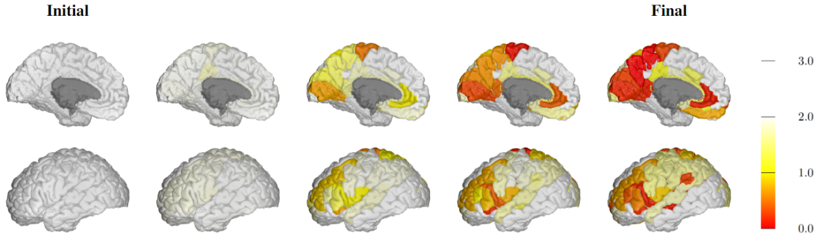
Figure 7: Visualization of adjustment of the trained scales on the cortical regions of a brain at training phase using FDG biomarker. Top: Inner part of left hemisphere, Bottom: Outer part of left hemisphere.

7. Adjustment of the learned scales

Fig. 7 displays the outcomes pertaining to the scale of each ROI in the brain during every quarter interval throughout the complete iteration within node-wise method. In contrast to prior approaches such as GraphHeat (Xu et al. 2020) and ADC (Zhao et al. 2021), which employ a uniform global scale for all regions of interest (ROIs), our proposed method looks for multivariate scales for each individual ROI during the training stage. The initial scales for all ROIs are uniformly set to the same value, and subsequently tuned to align with the corresponding data. As the learning phase progresses from its initial state, several ROIs associated with AD become spotlighted, which are colored by close to red in Fig. 7.

8. Discussions

Reasons for evaluating LSAP on the ADNI data. ADNI dataset was a suitable bench mark for the following reasons: 1) As the performance of node-wise scale training is sufficiently validated on node-classification with well-curated benchmarks, we wanted to run experiments on a real dataset with a practical application for scientific discovery such as Neuroimaging. 2) Brain has a common structure that can be translated to registered ROIs (i.e., nodes), where the results from LSAP can be clinically interpreted and convey interesting results to the readers. 3) ADNI study provide relatively large sample-size, and we have performed experiments with 5-fold cross validation to ensure unbiased results even though we are using only one dataset.

Limitations of LSAP. As LSAP needs to localize and update the scale for each node, training takes longer compared to conventional GNN that perform uniform convolution across all nodes, but this issue is well-addressed with our training on the scales within approximation. Another limitation is that LSAP operates with fixed set of nodes for graph classification. However, such a setting has an advantage with LSAP as we learn node-wise scale which yield interpretable results that may lead to scientific discoveries.

References

- Bailly et al. (2015) Bailly, M.; Destrieux, C.; Hommet, C.; Mondon, K.; Cottier, J.-P.; Beaufils, E.; Vierron, E.; Vercouillie, J.; Ibazizene, M.; Voisin, T.; et al. 2015. Precuneus and cingulate cortex atrophy and hypometabolism in patients with Alzheimer’s disease and mild cognitive impairment: MRI and 18F-FDG PET quantitative analysis using FreeSurfer. BioMed research international, 2015.
- Bastings et al. (2017) Bastings, J.; Titov, I.; Aziz, W.; Marcheggiani, D.; and Sima’an, K. 2017. Graph Convolutional Encoders for Syntax-aware Neural Machine Translation. In EMNLP, 1957–1967. Copenhagen, Denmark: Association for Computational Linguistics.
- Chamberlain et al. (2021) Chamberlain; et al. 2021. Grand: Graph neural diffusion. In ICML, 1407–1418. PMLR.
- Chen et al. (2018) Chen; et al. 2018. Fastgcn: fast learning with graph convolutional networks via importance sampling. ICLR.
- Chen et al. (2020) Chen; et al. 2020. Simple and deep graph convolutional networks. In International Conference on Machine Learning, 1725–1735. PMLR.
- Chen et al. (2021) Chen; et al. 2021. Deep iterative and adaptive learning for graph neural networks. AAAI.
- Chung et al. (1997) Chung; et al. 1997. Spectral graph theory, volume 92. American Mathematical Soc.
- de Jong et al. (2008) de Jong, L. W.; van der Hiele, K.; Veer, I. M.; Houwing, J.; Westendorp, R.; Bollen, E.; de Bruin, P. W.; Middelkoop, H.; van Buchem, M. A.; and van der Grond, J. 2008. Strongly reduced volumes of putamen and thalamus in Alzheimer’s disease: an MRI study. Brain, 131(12): 3277–3285.
- Destrieux et al. (2010) Destrieux; et al. 2010. Automatic parcellation of human cortical gyri and sulci using standard anatomical nomenclature. Neuroimage, 53(1): 1–15.
- Feng et al. (2020) Feng, W.; Zhang, J.; Dong, Y.; Han, Y.; Luan, H.; Xu, Q.; Yang, Q.; Kharlamov, E.; and Tang, J. 2020. Graph random neural networks for semi-supervised learning on graphs. NeurIPS, 33: 22092–22103.
- Galton et al. (2001) Galton, C. J.; Patterson, K.; Graham, K.; Lambon-Ralph, M. A.; Williams, G.; Antoun, N.; Sahakian, B.; and Hodges, J. 2001. Differing patterns of temporal atrophy in Alzheimer’s disease and semantic dementia. Neurology, 57(2): 216–225.
- Gao et al. (2019) Gao; et al. 2019. Graph u-nets. In international conference on machine learning, 2083–2092. PMLR.
- Guo et al. (2023) Guo; et al. 2023. Graph Neural Networks with Diverse Spectral Filtering. In WWW.
- Hammond et al. (2011) Hammond; et al. 2011. Wavelets on graphs via spectral graph theory. Applied and Computational Harmonic Analysis, 30(2): 129–150.
- He et al. (2022) He; et al. 2022. Convolutional Neural Networks on Graphs with Chebyshev Approximation, Revisited. NeurIPS.
- He et al. (2016) He, K.; Zhang, X.; Ren, S.; and Sun, J. 2016. Deep residual learning for image recognition. In CVPR, 770–778.
- Hoesen et al. (2000) Hoesen, V.; et al. 2000. Orbitofrontal cortex pathology in Alzheimer’s disease. Cerebral Cortex, 10(3): 243–251.
- Huang et al. (2020) Huang; et al. 2020. Fast polynomial approximation of heat kernel convolution on manifolds and its application to brain sulcal and gyral graph pattern analysis. IEEE transactions on medical imaging, 39(6): 2201–2212.
- Huang et al. (2023) Huang; et al. 2023. Node-wise Diffusion for Scalable Graph Learning. In WWW.
- Huang et al. (2019) Huang, L.; Ma, D.; Li, S.; Zhang, X.; and Wang, H. 2019. Text level graph neural network for text classification. EMNLP-IJCNLP.
- Kim et al. (2022) Kim; et al. 2022. How to find your friendly neighborhood: Graph attention design with self-supervision. ICLR.
- Kipf et al. (2017) Kipf; et al. 2017. Semi-supervised classification with graph convolutional networks. ICLR.
- Klicpera et al. (2019a) Klicpera; et al. 2019a. Diffusion improves graph learning. NeurIPS.
- Klicpera et al. (2019b) Klicpera; et al. 2019b. Predict then propagate: Graph neural networks meet personalized pagerank. ICLR.
- Lee et al. (2023) Lee; et al. 2023. Time-aware random walk diffusion to improve dynamic graph learning. In AAAI.
- Lin et al. (2021) Lin; et al. 2021. Medley: Predicting Social Trust in Time-Varying Online Social Networks. In IEEE INFOCOM 2021-IEEE Conference on Computer Communications, 1–10. IEEE.
- Lin, Gao, and Li (2020) Lin, W.; Gao, Z.; and Li, B. 2020. Shoestring: Graph-based semi-supervised classification with severely limited labeled data. In CVPR, 4174–4182.
- Liu et al. (2016) Liu; et al. 2016. Graph-based semisupervised learning for acoustic modeling in automatic speech recognition. IEEE/ACM Transactions on Audio, Speech, and Language Processing, 24(11): 1946–1956.
- Liu et al. (2020) Liu; et al. 2020. Towards deeper graph neural networks. In KDD, 338–348.
- Luo et al. (2022) Luo, Y.; Luo, G.; Yan, K.; and Chen, A. 2022. Inferring from References with Differences for Semi-Supervised Node Classification on Graphs. Mathematics, 10(8): 1262.
- Olver et al. (2010) Olver, F. W.; Lozier, D. W.; Boisvert, R. F.; and Clark, C. W. 2010. NIST handbook of mathematical functions hardback and CD-ROM. Cambridge university press.
- Oppenheim et al. (1997) Oppenheim, A. V.; Buck, J.; Daniel, M.; Willsky, A. S.; Nawab, S. H.; and Singer, A. 1997. Signals & systems. Pearson Educación.
- Page et al. (1999) Page, L.; Brin, S.; Motwani, R.; and Winograd, T. 1999. The PageRank citation ranking: Bringing order to the web. Technical report, Stanford InfoLab.
- Qi et al. (2017) Qi, X.; Liao, R.; Jia, J.; Fidler, S.; and Urtasun, R. 2017. 3d graph neural networks for rgbd semantic segmentation. In ICCV, 5199–5208.
- Sen et al. (2008) Sen, P.; Namata, G.; Bilgic, M.; Getoor, L.; Galligher, B.; and Eliassi-Rad, T. 2008. Collective classification in network data. AI magazine, 29(3): 93–93.
- Shchur et al. (2018) Shchur, O.; Mumme, M.; Bojchevski, A.; and Günnemann, S. 2018. Pitfalls of Graph Neural Network Evaluation. NeurIPS.
- Veličković et al. (2018) Veličković, P.; Cucurull, G.; Casanova, A.; Romero, A.; Lio, P.; and Bengio, Y. 2018. Graph attention networks. ICLR.
- Verma et al. (2018) Verma; et al. 2018. Feastnet: Feature-steered graph convolutions for 3d shape analysis. In CVPR.
- Wei et al. (2020) Wei; et al. 2020. View-gcn: View-based graph convolutional network for 3d shape analysis. In CVPR, 1850–1859.
- Wu et al. (2019) Wu; et al. 2019. Simplifying graph convolutional networks. In ICML, 6861–6871. PMLR.
- Wu et al. (2022a) Wu; et al. 2022a. Nodeformer: A scalable graph structure learning transformer for node classification. NeurIPS, 35: 27387–27401.
- Wu et al. (2022b) Wu, J.; Chen, X.; Xu, K.; and Li, S. 2022b. Structural entropy guided graph hierarchical pooling. In International Conference on Machine Learning, 24017–24030. PMLR.
- Xie et al. (2021) Xie, G.-S.; Liu, J.; Xiong, H.; and Shao, L. 2021. Scale-aware graph neural network for few-shot semantic segmentation. In CVPR, 5475–5484.
- Xu et al. (2020) Xu, B.; Shen, H.; Cao, Q.; Cen, K.; and Cheng, X. 2020. Graph convolutional networks using heat kernel for semi-supervised learning. IJCAI.
- Yang et al. (2021) Yang, X.; Deng, C.; Dang, Z.; Wei, K.; and Yan, J. 2021. SelfSAGCN: self-supervised semantic alignment for graph convolution network. In CVPR, 16775–16784.
- Zhang et al. (2019a) Zhang; et al. 2019a. Bayesian graph convolutional neural networks for semi-supervised classification. In AAAI, volume 33, 5829–5836.
- Zhang et al. (2019b) Zhang; et al. 2019b. ProNE: Fast and Scalable Network Representation Learning. In IJCAI, volume 19, 4278–4284.
- Zhang et al. (2023) Zhang; et al. 2023. ApeGNN: Node-Wise Adaptive Aggregation in GNNs for Recommendation. In WWW.
- Zhao et al. (2021) Zhao; et al. 2021. Adaptive diffusion in graph neural networks. NeurIPS, 34: 23321–23333.