Rethinking Centered Kernel Alignment in Knowledge Distillation

Abstract

Knowledge distillation has emerged as a highly effective method for bridging the representation discrepancy between large-scale models and lightweight models. Prevalent approaches involve leveraging appropriate metrics to minimize the divergence or distance between the knowledge extracted from the teacher model and the knowledge learned by the student model. Centered Kernel Alignment (CKA) is widely used to measure representation similarity and has been applied in several knowledge distillation methods. However, these methods are complex and fail to uncover the essence of CKA, thus not answering the question of how to use CKA to achieve simple and effective distillation properly. This paper first provides a theoretical perspective to illustrate the effectiveness of CKA, which decouples CKA to the upper bound of Maximum Mean Discrepancy (MMD) and a constant term. Drawing from this, we propose a novel Relation-Centered Kernel Alignment (RCKA) framework, which practically establishes a connection between CKA and MMD. Furthermore, we dynamically customize the application of CKA based on the characteristics of each task, with less computational source yet comparable performance than the previous methods. The extensive experiments on the CIFAR-100, ImageNet-1k, and MS-COCO demonstrate that our method achieves state-of-the-art performance on almost all teacher-student pairs for image classification and object detection, validating the effectiveness of our approaches.

1 Introduction

Tremendous efforts have been made in compressing large-scale models into lightweight models. Representative methods include network pruning Frankle and Carbin (2019), model quantization Wu et al. (2016), neural architecture search Wan et al. (2020) and knowledge distillation (KD) Hinton et al. (2015). Among them, KD has recently emerged as one of the most flourishing topics due to its effectiveness Liu et al. (2021b); Huang et al. (2022); Gong et al. (2023); Shao et al. (2023a) and wide applications Chong et al. (2022); Chen et al. (2023); Shao et al. (2023b). Particularly, the core idea of KD is to transfer the acquired representations from a large-scale and high-performing model to a lightweight model by distilling the learning representations in a compact form, achieving precision and reliable knowledge transfer. Out of the consensus of researchers, there are two mainstream approaches to distilling knowledge from the teacher to the student. The first approach is the logit-based distillation, which aims to minimize the probabilistic prediction (response) scores between the teacher and student by leveraging appropriate metrics Zhao et al. (2022); Hinton et al. (2015). The other is feature-based distillation, which investigates the knowledge within intermediate representations to further boost the distillation performance Yang et al. (2022b); Liu et al. (2021a); Chen et al. (2021); Ahn et al. (2019). Among them, the design of metrics is essential in knowledge transfer and has been attractive to scholars. Kornblith at al Kornblith et al. (2019) proposes the Centered Kernel Alignment (CKA) for the quantitative understanding of representations between neural networks. CKA not only focuses on model predictions but also emphasizes high-order feature representations within the models, providing a comprehensive and enriched knowledge transfer.

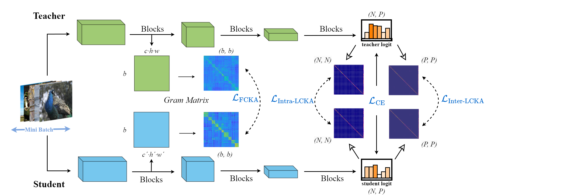
Figure 1: The overall framework of the proposed Relation-based Centered Kernel Alignment (RCKA). We first transform the feature map from the shape of $(B,C,HW)$ into $(B,CHW)$ and then compute the CKA similarity of feature maps between the teacher and the student. Besides, we compute the inter-class and intra-class CKA similarity of logits between teacher and student. Here, $N$ refers to the number of samples, and $P$ refers to the corresponding probability of class to which this sample belongs.

Recent studies Qiu et al. (2022); Saha et al. (2022) introduce CKA to quantitatively narrow the gap of learned representations between the teacher model and the student model. Undeniably, these methods have achieved significant success. However, their designs are excessively complex and need a large amount of computational resources, making it challenging to achieve fine-grained knowledge transfer and leading to low scalability. Moreover, these methods fail to uncover the essence of CKA, lacking an in-depth analysis of CKA in knowledge distillation. The reason why CKA is effective has not been explored. Therefore, we focus on the theoretical analysis of CKA and rethink a more reasonable architecture design that ensures simplicity and effectiveness while generalizing well across various tasks.

In this paper, we provide a novel perspective to illustrate the effectiveness of CKA, where CKA is regarded as the upper bound of Maximum Mean Discrepancy (MMD) with a constant term, specifically. Drawing from this, we propose a Relation-Centered Kernel Alignment (RCKA) framework, which practically establishes a connection between CKA and MMD. Besides, we dynamically customize the application of CKA on instance-level tasks, and introduce Patch-based Centered Kernel Alignment (PCKA), with less computational source yet competitive performance when compared to previous methods. Our method is directly applied not only to logit-based distillation but also to feature-based distillation, which exhibits superior scalability and expansion. We utilize CKA to compute high-order representation information both between and within categories, which better motivates the alleviation of the performance gap between the teacher and student.

To validate the effectiveness of our approaches, we conduct extensive experiments on image classification (CIFAR-100 Krizhevsky and Hinton (2009) and ImageNet-1k Russakovsky et al. (2015)), and object detection (MS-COCO Lin et al. (2014)) tasks. As a result, our methods achieve state-of-the-art (SOTA) performance in almost all quantitative comparison experiments with fair comparison. Moreover, following our processing architecture, the performance of the previous distillation methods is further boosted in the object detection task.

Our contribution can be summarized as follows:

• We rethink CKA in knowledge distillation from a novel perspective, providing a theoretical reason for why CKA is effective in knowledge distillation.

• We propose a Relation Centered Kernel Alignment (RCKA) framework to construct the relationship between CKA and MMD, with less computational source yet comparable performance than previous methods, which verifies our theoretical analysis correctly.

• We further dynamically customize the application of CKA for instance-level tasks and propose a Patch-based Centered Kernel Alignment (PCKA) architecture for knowledge distillation in object detection, which further boosts the performance of previous distillation methods.

• We conduct plenty of ablation studies to verify the effectiveness of our method, which achieves SOTA performance on a range of vision tasks. Besides, we visualize the characteristic information of CKA and discover new patterns in it.

2 Related Work

Vanilla Knowledge Distillation Hinton et al. (2015) proposes aligning the output distributions of classifiers between the teacher and student by minimizing the KL-divergence, during training the emphasis on negative logits can be fine-tuned through a temperature coefficient, which serves as a form of normalization during the training process of a smaller student network. Tremendous efforts Tung and Mori (2019); Huang et al. (2022); Qiu et al. (2022); Zagoruyko and Komodakis (2016a); Park et al. (2019) have been made on how to design a good metric to align the distribution between the teacher and student.

Design an suitable alignment method for KD can start from two typical types: Drawing on representations, numerous methods have made significant strides by aligning the intermediate features Zagoruyko and Komodakis (2016a), the samples’ correlation matrices Tung and Mori (2019), and the output logits between the teacher and student Huang et al. (2022). From a mathematical standpoint, some measure theories are introduced to illustrate the similarity between the teacher and student, such as mutual information Ahn et al. (2019). Among these, Centered Kernel Alignment (CKA) is a valuable function for measuring similarity. It simultaneously considers various properties during similarity measures, such as invariance to orthogonal transformations. While the effectiveness of CKA in KD has been demonstrated in some works Qiu et al. (2022); Saha et al. (2022), the essence of CKA has not been thoroughly explored, and the unavoidable additional computational costs also limit its application prospect.

In this paper, we will revisit CKA in KD and provide a novel theoretical perspective to prove its effectiveness and analyze how it functions across various distillation settings.

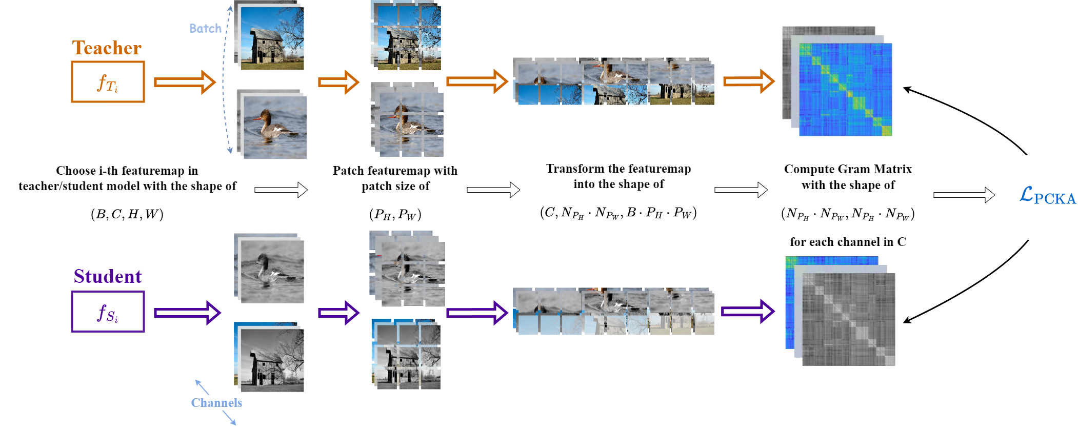
Figure 2: The overall framework of PCKA. We dynamically customize the framework of proposed method based on the characteristics of object detection. In this framework, we first patch the featuremap of the teacher and student with the patchsize $(P_{H},P_{W})$, then transform the featuremap in order to get the gram matrix between each patch. Finally, we calculate the loss $L_{PCKA}$, and get average from dimension $C$. Here, $B,C,H,W$ refer to the batchsize, channels, height and width of the featuremap, respectively. $N_{P_{H}},N_{P_{W}}$ denote the number of patches cutting along the height and width, respectively.

3 Methodolgy

Table 1: Results on the CIFAR-100 test set. “Same” and “Different” in the first row refer to whether the model architecture is the same for teachers and students. Combined distillation type means that this method transfers the knowledge both on the features and logits. Our methods surpass almost all algorithms with the same distillation type. “RN”, “WRN”, “SN”, and “MN” denote ResNet, Wide ResNet, ShuffleNet, and MobileNet, respectively.

Architecture		Same						Different
Distillation Type	Teacher	RN-110	RN-110	WRN-40-2	WRN-40-2	RN-32$\times$4	VGG-13	WRN-40-2	RN-32$\times$4	VGG-13
		74.31	74.31	75.61	75.61	79.42	74.64	75.61	79.42	74.64
	Student	RN-20	RN-32	WRN-40-1	WRN-16-2	RN-8$\times$4	VGG-8	SN–V1	SN–V1	MN–V2
		69.06	71.14	71.98	73.26	72.50	70.36	70.50	70.50	64.60
Feature-based	FitNet Romero et al. (2014)	68.99	71.06	72.24	73.58	73.50	71.02	73.73	73.59	64.14
	ATKD Zagoruyko and Komodakis (2016a)	70.22	70.55	72.77	74.08	73.44	71.43	73.32	72.73	59.40
	SPKD Tung and Mori (2019)	70.04	72.69	72.43	73.83	72.94	72.68	74.52	73.48	66.30
	CCKD Peng et al. (2019)	69.48	71.48	72.21	73.56	72.97	70.71	71.38	71.14	64.86
	RKD Park et al. (2019)	69.25	71.82	72.22	73.35	71.90	71.48	72.21	72.28	64.52
	VID Ahn et al. (2019)	70.16	70.38	73.30	74.11	73.09	71.23	73.61	73.38	65.56
	CRD Tian et al. (2020)	71.46	73.48	74.14	75.48	75.51	73.94	76.05	75.11	69.73
	OFD Heo et al. (2019)	-	73.23	74.33	75.24	74.95	73.95	75.85	75.98	69.48
	ReviewKD Chen et al. (2021)	-	71.89	75.09	76.12	75.63	74.84	77.14	76.93	70.37
	ICKD-C Liu et al. (2021a)	71.91	74.11	74.63	75.57	75.48	73.88	75.19	74.34	67.55
	DPK Qiu et al. (2022)	72.44	74.89	75.27	76.42	-	74.96	74.43	76.00	68.63
	FCKA(ours)	71.49	73.64	74.70	75.53	74.93	74.35	75.98	75.67	68.97
Logit-based	KD Hinton et al. (2015)	70.67	73.08	73.54	74.92	73.33	72.98	74.83	74.07	67.37
	DKD Zhao et al. (2022)	-	74.11	74.81	76.24	76.32	74.68	76.70	76.45	69.71
	DIST Huang et al. (2022)	69.94	73.55	74.42	75.29	75.79	73.74	75.23	75.23	68.48
	IKL-KD Cui et al. (2023)	-	74.26	74.98	76.45	76.59	74.88	77.19	76.64	70.40
	NKD Yang et al. (2023)	71.26	73.79	75.23	76.37	76.35	74.86	76.59	76.90	70.22
	LCKA(ours)	70.87	73.64	74.63	75.78	75.12	74.35	76.12	76.43	69.37
Combined	SRRL Yang et al. (2021)	71.51	73.80	74.75	75.96	75.92	74.40	76.61	75.66	69.14
	RCKA(ours)	72.26	74.31	75.34	76.51	76.11	74.97	77.21	76.97	70.12

In this section, we first revisit the paradigm of knowledge distillation and then introduce the formula of Centered Kernel Alignment (CKA). Specifically, we derive the formula of the relationship between CKA and Maximum Mean Discrepancy (MMD), where CKA can be decoupled as the upper bound of MMD with a constant term. In light of the above deduction, we outline the methodology of our paper. We apply the proposed methods in image classification and object detection, dynamically customizing CKA for each task.

3.1 The Paradigm of Knowledge Distillation

The existing KD methods can be categorized into two groups. Particularly, the logits-based KD methods narrow the gap between the teacher and student models by aligning the soft targets between them, which is formulated as following loss term:

$$L_{\mathrm{logits}}=\mathsf{D}_{\mathrm{logits}}(\mathsf{T}_{s}(\sigma(z_{s};\tau)),\mathsf{T}_{t}(\sigma(z_{t};\tau))),$$ (1)

where $z_{s}$ and $z_{t}$ are the logits from students and teachers, respectively. And $\sigma(\cdot)$ is the softmax function that produces the category probabilities from the logits, and $\tau$ is a non-negative temperature hyper-parameter to scale the smoothness of the predictive distribution. Specifically, we have $\sigma_{i}(z;\tau)=\operatorname{softmax}(\exp(z_{i}/\tau))$. $\mathsf{D}_{\mathrm{logits}}$ is a loss function to capture the discrepancy distributions, e.g. Kullback-Leibler divergence. And $\mathsf{T}_{s}$ and $\mathsf{T}_{t}$ denote the transformation functions in students and teachers, respectively, which usually refer to the identity mapping in Vanilla KD Hinton et al. (2015).

Similarly, the feature-based KD methods, which aim to mimic the feature representations between teachers and students, are also represented as a loss item:

$$L_{\mathrm{feat}}=D_{\mathrm{feat}}(\mathsf{T}_{s}(\mathbf{F}_{s}),\mathsf{T}_{t}(\mathbf{F}_{t})),$$ (2)

where $\mathbf{F}_{s}$ and $\mathbf{F}_{t}$ denote feature maps from students and teachers, respectively. Transformation modules $\mathsf{T}_{s}$ and $\mathsf{T}_{t}$ align the dimensions of $\mathbf{F}_{s}$ and $\mathbf{F}_{t}$. $D_{\mathrm{feat}}$ computes the distance between two feature maps, such as $\ell_{1}$- or $\ell_{2}$ norm. Therefore, the KD methods can be represented by a generic paradigm. The final loss is the weighted sum of the cross-entropy loss $L_{ce}$, the logits distillation loss, and the feature distillation loss:

$$L=L_{ce}+\alpha L_{\mathrm{logits}}+\beta L_{\mathrm{feat}},$$ (3)

where $\alpha$ and $\beta$ are hyper-parameters controlling the trade-off between these three losses.

3.2 Distilling with the Upper Bound

Centered Kernel Alignment (CKA) has been proposed as a robust way to measure representational similarity between neural networks. We first prove that CKA measures the cosine similarity of the gram matrix between teachers and students.

Theorem 1 (Proof in Appendix C.1).

Let $X$ and $Y$ be $N\times P$ matrices. The CKA similarity $\|Y^{\top}X\|_{F}^{2}$ is equivalent to the cosine similarity of $XX^{\top}$ and $YY^{\top}$, which denote the gram matrix of $X$ and $Y$, respectively. In other words,

$$S_{\mathrm{CKA}}(X,Y) =\frac{\|Y^{\top}X\|_{F}^{2}}{\|X^{T}X\|_{F}\|Y^{T}Y\|_{F}}$$

$$=\frac{\mathrm{vec}(XX^{\top})^{\top}\mathrm{vec}(YY^{\top})}{\|\mathrm{vec}(XX^{\top})\|_{2}\|\mathrm{vec}(YY^{\top})\|_{2}},$$

where $\mathrm{vec}$ operator represents reshaping the matrix to a vector.

We then derive the formula of the relationship between CKA and MMD, where CKA can be regarded as the upper bound of MMD with a constant term.

Theorem 2 (Proof in Appendix C.2).

Maximizing CKA similarity is equivalent to minimizing the upper bound of MMD distance:

$$\frac{\|Y^{\top}X\|_{F}^{2}}{\|X^{T}X\|_{F}\|Y^{T}Y\|_{F}}=-N\mathbb{E}_{i,j}[\left<x_{i},x_{j}\right>-\left<y_{i},y_{j}\right>]^{2}+2$$

$$\leq-N\left(\mathbb{E}_{i,j}[\left<x_{i},x_{j}\right>]-\mathbb{E}_{i,j}[\left<y_{i},y_{j}\right>]\right)^{2}+2,$$

where the inequality is given by Jesen’s inequality.

According to Jesen’s inequality, CKA can be decoupled as the upper bound of MMD with a constant term. The first term corresponds to minimizing the upper bound of MMD distance with the RKHS kernel. In contrast, the latter constant term acts as a weight regularizer, enhancing the influence of MMD, where it promotes the similarity between features of the same batch, not only instances in the same class but also in different classes. On one hand, optimizing the upper bound of MMD, which has additional stronger constraints, allows it to converge to the optimal solution more quickly and stably. On the other hand, the latter term serves as a weight scaling mechanism, effectively avoiding the challenges of optimization caused by excessively small MMD values, which result in small gradients.

According to the deduction, we successfully transformed our optimization objective from maximizing CKA to minimizing the upper bound of MMD, which makes our method more intuitive and concise. Building upon these findings, we propose our methods, which are more effective than previous methods.

3.3 Relation-based Centered Kernel Alignment

As illustrated in Fig. 1, we propose a Relation Centered Kernel Alignment (RCKA) framework in image classification. In this framework, we leverage CKA as a loss function to ensure that the centered similarity matrix is distilled rather than forcing the student to mimic the teacher‘s similarity matrix with a different scale. This is very important because a model‘s discriminative capability is dependent on the distribution of its features rather than its scale, which is inconsequential for class separation Nguyen et al. (2020); Orhan and Pitkow (2017).

Assume we have a large-scale teacher model $t$ and a lightweight student model $s$. The activation map from layer $l$ of the teacher is denoted as $F^{(l)}_{t}\in\mathbb{R}^{b\times c\times h\times w}$, whereas the activation map of layer $l^{\prime}$ of the student is denoted as $F^{(l^{\prime})}_{s}\in\mathbb{R}^{b\times c^{\prime}\times h^{\prime}\times w^{\prime}}$. $c$, $h$, and $w$ denote the channel, height, and width of the teacher, whereas $c^{\prime},h^{\prime}$ and $w^{\prime}$ denote that of the student. The mini-batch size is denoted by $b$. The logits of the teacher and student are denoted as $z_{t}\in\mathbb{R}^{N\times P}$ and $z_{s}\in\mathbb{R}^{N\times P^{\prime}}$, where $N$ and $P$ (or $P^{\prime}$) refer to the number of samples and the corresponding probability for which class this sample belongs to. Therefore, the formula of our method, similar to Eqn. 3, is represented as:

$$L_{\mathrm{RCKA}} =L_{CE}+\alpha L_{\mathrm{FCKA}}$$ (4)

$$+\beta(L_{\mathrm{Intra-LCKA}}+L_{\mathrm{Inter-LCKA}})$$ (5)

where $\alpha$ and $\beta$ are hyper-parameters controlling the trade-off between the features loss $L_{\mathrm{FCKA}}$ and logits loss $(L_{\mathrm{Intra-LCKA}}+L_{\mathrm{Inter-LCKA}})$.

The $L_{\mathrm{FCKA}}$, $L_{\mathrm{Intra-LCKA}}$ and $L_{\mathrm{Inter-LCKA}}$ are represented as:

$$L_{\mathrm{FCKA}}=S_{\mathrm{CKA}}(\mathsf{T}(\mathbf{F}_{t}),\mathsf{T}(\mathbf{F}_{s})),$$ (6)

$$L_{\mathrm{Intra-LCKA}}=S_{\mathrm{CKA}}(z_{t},z_{s}),$$ (7)

$$L_{\mathrm{Inter-LCKA}}=S_{\mathrm{CKA}}(z_{t}^{\mathsf{T}},z_{s}^{\mathsf{T}}),$$ (8)

where $\mathsf{T}$ in Eqn. 6 refers to the transformation module $\mathbb{R}^{b\times c\times h\times w}\rightarrow\mathbb{R}^{b\times chw}$.

Compared with the previous methods, our method has superior scalability and expansion and can be directly applied to both feature and logits distillation. We calculate the gram matrix to collect high-order inter-class and intra-class representations, encouraging the student to learn more useful knowledge. Also, we provide the relationship between CKA and MMD in Appendix C.2 to better demonstrate the theoretical support of our method.

Because the value of CKA ranges from $[0,1]$, at the beginning of the training process, $L_{CE}$ plays a more important role than all CKA losses to drive the optimization of the student, which helps the student avoid matching extremely complex representations.

Table 2: Results on the ImageNet validation set. We use ResNet-34 and ResNet-50 released by Torchvision Marcel and Rodriguez (2010) as our teacher’s pre-training weight.

Architecture			Accuracy		Feature-based					Logit-based				Combined
Teacher	Student		Teacher	Student	OFD	CRD	ReviewKD	ICKD-C	MGD Yang et al. (2022b)	KD	RKD	DKD	DIST	SRRL	Ours
ResNet-34	ResNet-18	Top-1	73.31	69.76	71.08	71.17	71.61	72.19	71.80	70.66	70.34	71.70	72.07	71.73	72.34
		Top-5	91.42	89.08	90.07	90.13	90.51	90.72	90.40	89.88	90.37	90.41	90.42	90.60	90.68
ResNet-50	MobileNet-V1	Top-1	76.16	70.13	71.25	71.37	72.56	-	72.59	70.68	-	72.05	73.24	72.49	72.79
		Top-5	92.86	89.49	90.34	90.41	91.00	-	90.74	90.30	-	91.05	91.12	90.92	91.01

Table 3: Results on the COCO validation set (T$\rightarrow$S refers to the distillation from T to S). Here, the content in brackets to the right of “Ours” refers to the methods applied in the distillation process. In addition, CM RCNN-X101 stands for Cascade Mask RCNN-X101.

T$\rightarrow$S	CM RCNN-X101 Cai and Vasconcelos (2017)$\rightarrow$Faster RCNN-R50 Ren et al. (2015)						RetinaNet-X101$\rightarrow$RetinaNet-R50 Lin et al. (2017)							T$\rightarrow$S	FCOS-R101$\rightarrow$FCOS-R50 Tian et al. (2019)
Type	Two-stage detectors						One-stage detectors							Type	Anchor-free detectors
Method	AP	AP50	AP75	APS	APM	APL	AP	AP50	AP75	APS	APM	APL		Method	AP	AP50	AP75	APS	APM	APL
Teacher	45.6	64.1	49.7	26.2	49.6	60.0	41.0	60.9	44.0	23.9	45.2	54.0		Teacher	40.8	60.0	44.0	24.2	44.3	52.4
Student	38.4	59.0	42.0	21.5	42.1	50.3	37.4	56.7	39.6	20.0	40.7	49.7		Student	38.5	57.7	41.0	21.9	42.8	48.6
KD Hinton et al. (2015)	39.7	61.2	43.0	23.2	43.3	51.7	37.2	56.5	39.3	20.4	40.4	49.5		KD Hinton et al. (2015)	39.9	58.4	42.8	23.6	44.0	51.1
COFD Heo et al. (2019)	38.9	60.1	42.6	21.8	42.7	50.7	37.8	58.3	41.1	21.6	41.2	48.3		FitNet Romero et al. (2014)	39.9	58.6	43.1	23.1	43.4	52.2
FKD Zhang and Ma (2021)	41.5	62.2	45.1	23.5	45.0	55.3	39.6	58.8	42.1	22.7	43.3	52.5		GID Dai et al. (2021)	42.0	60.4	45.5	25.6	45.8	54.2
DIST Huang et al. (2022)	40.4	61.7	43.8	23.9	44.6	52.6	39.8	59.5	42.5	22.0	43.7	53.0		FRS Zhixing et al. (2021)	40.9	60.3	43.6	25.7	45.2	51.2
DIST+mimic Huang et al. (2022)	41.8	62.4	45.6	23.4	46.1	55.0	40.1	59.4	43.0	23.2	44.0	53.6		FGD Yang et al. (2022a)	42.1	-	-	27.0	46.0	54.6
Ours	41.4	62.1	45.2	23.5	45.6	54.9	40.3	59.9	43.0	23.3	44.2	54.9		Ours	39.8	59.0	42.4	22.2	43.6	52.5
Ours + mimic	42.4	63.3	46.1	24.3	46.7	56.1	40.7	60.4	43.4	23.9	44.7	55.1		Ours + mimic	40.7	60.5	43.1	23.4	44.8	53.1

3.4 Patch-based Centered Kernel Alignment

In this subsection, we further adapt the proposed RCKA to instance-level tasks such as object detection. However, directly applying RCKA to instance-level tasks may deteriorate performance, as the above tasks are usually trained with a small size of mini-batches (e.g. $2$ or $4$ per GPU), causing the failure of the gram matrix to collect enough knowledge. Besides, increasing the mini-batch size requires a significant amount of computational resources, making it infeasible in practice. Thus, we dynamically customize our RCKA method for object detection.

Recent works Shu et al. (2021); Heo et al. (2019) find that distilling the representations of intermediate layers is more effective than distilling the logits in object detection. Therefore, we adjust our method to only target intermediate layers. Still, we follow our core idea in the classification task, which calculates the similarities between different instances by using CKA. So, we divide the image feature maps into several patches and compute the similarities between different patches.

Our redesigned method is illustrated in Fig. 2. In this framework, we first patch the feature maps of the teacher and student with a patch size of $(P_{H},P_{W})$, then transform the feature maps to get the gram matrix between each patch. Finally, we calculate the loss $L_{\mathrm{PCKA}}$ and get the average from dimension $C$. Here, $N_{P_{H}}$ and $N_{P_{W}}$ denote the number of patches cutting along the height and width, respectively. Therefore, the Patch-based CKA loss is represented as:

$$L_{\mathrm{PCKA}}=\gamma S_{\mathrm{CKA}}(N^{s}_{P_{H}}\cdot N^{s}_{P_{W}},N^{t}_{P_{H}}\cdot N^{t}_{P_{W}}),$$ (9)

where $N^{s}_{P_{H}}\cdot N^{s}_{P_{W}}$ and $N^{t}_{P_{H}},N^{t}_{P_{W}}$ are denoted as the number of the student patches and the teacher patches, respectively. Usually, $N^{s}_{P_{H}}\cdot N^{s}_{P_{W}}=N^{t}_{P_{H}},N^{t}_{P_{W}}$. $\gamma$ refers to the loss weight factor.

4 Experiments

We conduct extensive experiments on image classification and object detection benchmarks. The image classification datasets include CIFAR-100 Krizhevsky and Hinton (2009) and ImageNet-1k Russakovsky et al. (2015) and the object detection dataset includes MS-COCO Lin et al. (2014). Moreover, we present various ablations and analyses for the proposed methods. More details about these datasets are in Appendix A. We apply a batch size of $128$ and an initial learning rate of $0.1$ for the SGD optimizer on CIFAR-100. And we follow the settings in Huang et al. (2022) for the ResNet34-ResNet18 pair and the ResNet50-MobileNet pair on ImageNet-1k. The settings of other classification and detection tasks are in Appendix B. Our code will be publicly available for reproducibility.

4.1 Image Classification

Classification on CIFAR-100.

We compare state-of-the-art (SOTA) feature-based and logit-based distillation algorithms on 9 student-teacher pairs. Among them, $6$ pairs have the same structure for teachers and students, and the rest of them have different architectures. The results are presented in Tab. 1. Our proposed method outperforms all other algorithms on $4$ student-teacher pairs and achieves comparable performance on the rest of them, meanwhile requiring extremely less computational resources and time consumption than the SOTA methods DPK Qiu et al. (2022) and ReviewKD Chen et al. (2021). The comparisons of computational cost are in Appendix D.

Classification on ImageNet-1k.

We also conduct experiments on the large-scale ImageNet to evaluate our methods. Our RCKA achieves comparable results with other algorithms, even outperforms them, as shown in Tab. 2. We find that with the increasing of categories and instances, it is more challenging for the student to mimic the high-order distribution of the teacher. Moreover, in Appendix 8, we We explore the feature distillation for ViT-based models on ImageNet-1k. It is noted that our method outperforms other methods, which means that our method has good scalability and good performance.

Table 4: Results on the COCO validation set (T$\rightarrow$S refers to the distillation from T to S). Here, the content in brackets to the right of “Ours” refers to the methods applied in the distillation process. In addition, “Inside GT Box” means we use the GT boxes with the same stride on the FPN layers as the feature imitation regions. “Main Region” means we imitate the features within the main distillation region.

T$\rightarrow$S	GFL-R101$\rightarrow$GFL-R50  Li et al. (2020)
Method	AP	AP50	AP75	APS	APM	APL
Teacher	44.9	63.1	49.0	28.0	49.1	57.2
Student	40.2	58.4	43.3	23.3	44.0	52.2
FT Romero et al. (2014)	40.7	58.6	44.0	23.7	44.4	53.2
Inside GT Box	40.7	58.6	44.2	23.1	44.5	53.5
DeFeat	40.8	58.6	44.2	24.3	44.6	53.7
Main Region	41.1	58.7	44.4	24.1	44.6	53.6
FGFI Wang et al. (2019)	41.1	58.8	44.8	23.3	45.4	53.1
FGD Yang et al. (2022a)	41.3	58.8	44.8	24.5	45.6	53.0
GID Dai et al. (2021)	41.5	59.6	45.2	24.3	45.7	53.6
SKD de Rijk et al. (2022)	42.3	60.2	45.9	24.4	46.7	55.6
Our	42.8	61.2	46.3	24.8	47.1	55.4

4.2 Object Detection

Detection on MS-COCO.

Comparison experiments are run on three kinds of different detectors, i.e., tow-stage detectors, one-stage detectors, and anchor-free detectors. As shown in Tab. 3, PCKA outperforms the precious methods almost on all three kinds of metrics, by aligning the high-order patch-wise presentations. We believe that aligning feature maps of the student and teacher in low-order could also improve the performance of PCKA, driven by mimicking low-order representations in the early stage and then learning high-order and complex representations gradually. Thus, we follow Huang et al. (2022) by adding auxiliary mimic loss, i.e., translating the student feature maps from the teacher feature map by a convolution layer and supervising them utilizing $\mathcal{L}_{MSE}$, to the detection distillation task. Ultimately, we conclude from Tab. 3 that PCKA-based mimic loss achieves the best performance on Cascade RCNN-X101-Cascade RCNN-R50 and RetinaNet-X101-RetinaNet-R50 pairs. We also conduct experiments on the other four architectures, as shown in Tab. 4 and Tab. 9. These results further validate the effectiveness of our proposed method.

4.3 Ablations and Visualizations

We conduct ablation studies in three aspects: (a) the effect of hyper-parameters. (b) effectiveness of the proposed modules. (c) unexplored phenomenon during training.

Ablation studies on hyperparameters.

As shown in Tab. 12, Tab. 11 and Tab. 13 in Appendix, we conduct the ablation studies on the size of mini-batch, loss scaling factor $\gamma$ on $L_{PCKA}$ and the number of intermediate layers for distilling. We find the local optima values are the mini-batch size $12$, loss scaling factor $10$, and $3$ layers of distillation.

The upper bound of MMD.

In Theorem 2, we derive the relationship between CKA and MMD, where CKA is the upper bound of MMD with a constant term. To validate this, We conduct the experiment, which is shown in Tab. 6, we notice that CKA, which is the upper bound of MMD, has additional stronger constraints. Because of this, CKA converges to the optimal solution more quickly and stably, compared with MMD.

The dimension to average.

In PCKA framework, we cut the activations of the teacher and student in the shape of $(C,N_{P_{H}}\cdot N_{P_{W}},B\cdot P_{H}\cdot P_{W})$. We also carry out the experiments of averaging on different dimensions, shown in Tab. 5. We find averaging on channel dimension is the optima.

Patch distillation.

We explore the effectiveness of cutting activations into patches. As shown in Tab. 7, several standard distillation methods Hinton et al. (2015); Zagoruyko and Komodakis (2016a); Huang et al. (2022) all perform well with patch cutting, validating the effectiveness of cutting patches. With the smaller representation distribution in patches, it is easier to align the teacher and student. Thus, the proposed PCKA architecture amazingly boosts the previous methods.

Table 5: The ablation study on the COCO validation set (T$\rightarrow$S refers to the distillation from T to S). Here, we explore which dimension we should choose to get better results. ”Mix-up” means the 1st distilling layer uses Batch avg. method, the 2nd distilling layer uses Spatial avg. method and the final distilling layer uses Channel avg. method

T$\rightarrow$S	RetinaNet-X101$\rightarrow$RetinaNet-R50
Method	AP	AP50	AP75	APS	APM	APL
Teacher	41.0	60.9	44.0	23.9	45.2	54.0
Student	37.4	56.7	39.6	20.0	40.7	49.7
Batch avg.	38.5	57.9	40.8	20.7	41.5	52.5
Spatial avg.	39.3	58.7	41.9	21.4	41.3	50.9
Mix-up avg.	38.2	58.1	40.4	21.3	41.9	50.9
Channel avg.	40.3	59.9	43.0	23.3	44.2	54.9

Visualize the CKA value.

We present some visualizations to show that our method does bridge the teacher-student gap in logit-level. In particular, we visualize the logit similarity for $6$ teacher-student pairs in Appendix E. We find that our method significantly improves the logit-similarity.

Visualize the training process.

We further visualize the training process of different detectors and the patch effect on the RetinaNet-X101-RetinaNet-R50 pair. The results are in Tab. 4 and Tab. 3 in the Appendix.

Table 6: Experiments on the upper bound of MMD. We derive the formula that CKA is the upper bound of MMD with a constant term. From these experiments, we can prove that optimizing the upper bound of MMD can better improve the performance, compared with MMD.

T$\rightarrow$S	RetinaNet-X101$\rightarrow$RetinaNet-R50
Method	AP	AP50	AP75	APS	APM	APL
Teacher	41.0	60.9	44.0	23.9	45.2	54.0
Student	37.4	56.7	39.6	20.0	40.7	49.7
MMD w/ patch	38.5	57.7	40.9	22.2	42.8	51.3
PCKA	40.3	59.9	43.0	23.3	44.2	54.9

Visualize the inference outputs.

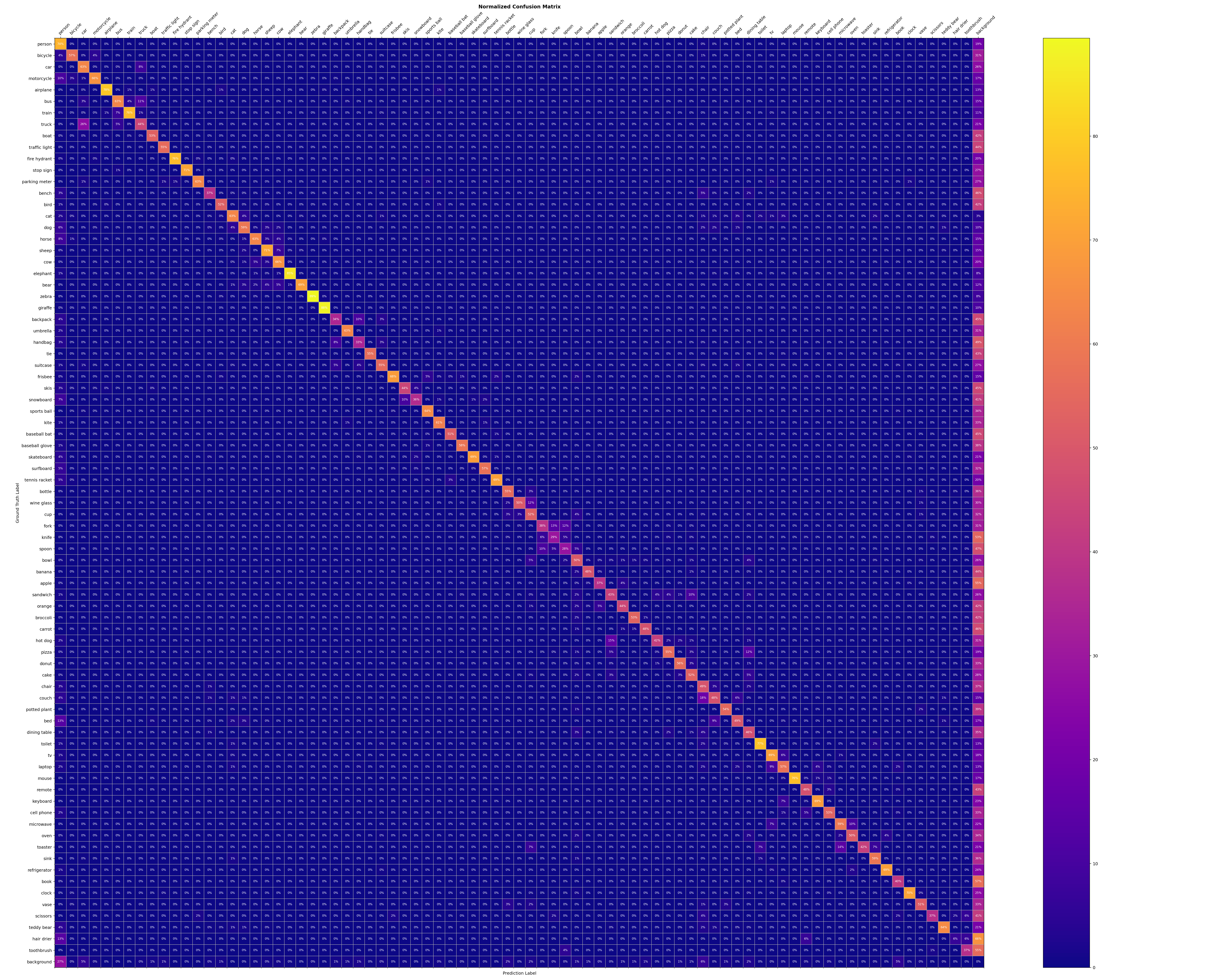
Figure 6: The confusion matrix is from the RetinaNet-R50, distilled by PCKA with teacher model RetinaNet-X101, averaging on channel.

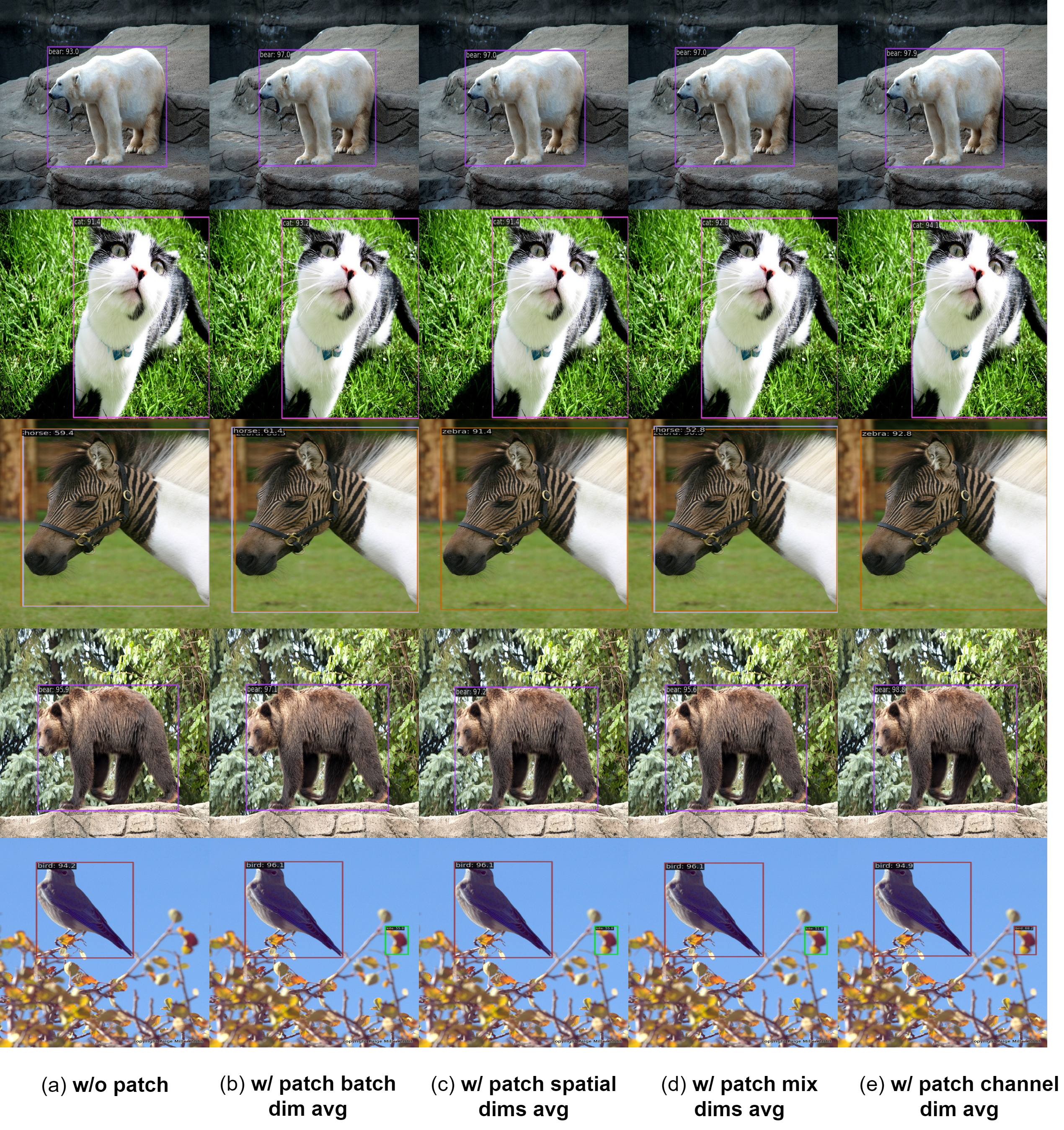
Figure 7: Top 5 inference results with RetinaNet-R50, distilled by PCKA without patch or with patch.

We first visualize the confusion matrix of the proposed method in Fig. 6, and then visualize the annotated images of training with/without patches averaging different dimensions in Fig. 7, respectively. These figures reveal that our method can collect the similarities between different classes, and also show the effectiveness of our method on the object detection task.

5 Discussion

PCKA in image classification.

We apply PCKA to the classification task, and it also outperforms well on the methods with the same distillation type, as shown in Tab. 14. However, PCKA performs very badly on the teacher-student pairs with different architectures. As cutting activations of different architectures contain more dissimilar and harmful representations, bringing difficulty in transferring knowledge to the student.

Average on the channel, boosting the performance.

The results in Tab. 7 reveal an interesting phenomenon, where the performance of the previous distillation methods is boosted by averaging the loss on channel dimension after the activations are cut into patches. Instead of directly matching the whole representation distribution in the activations, cutting patches makes the alignment between the teacher and student easier with a smaller representation distribution in patches. Besides, cutting into patches follows the idea in the framework of classification proposed by us, thus PCKA calculates the inter-class similarities and intra-class similarities in patches. Moreover, due to the superiority of cosine similarity over distance-based losses Boudiaf et al. (2020) and high-order distribution representations collected by the gram matrix, PCKA outperforms DIST and AT.

Positional information loss.

In PCKA, we cut the activation of the teacher and student into patches, and then flatten them into a vector. Although this operation damages the original positional information, performance does not deteriorate. We suppose that CKA ensures the focus of the optimization is on the shape of the distribution, rather than the raw values in the Gram matrix, which is vital because a model‘s discriminative capability is dependent on the distribution of its features rather than its scale. Besides, at the beginning, the effect brought by PCKA is smaller, compared with CE loss. Therefore, CE loss motivates the optimization of the student model steadily, and starting from a certain moment, PCKA drives the student model to align complex and high-order representations, improving the generalization ability.

Table 7: Ablation study of distillation methods with(w/) or without(w/o) patch on the COCO validation set (T$\rightarrow$S refers to the distillation from T to S). Here, we surprisingly notice that previous distillation method performance can be improved by image patching.

T$\rightarrow$S	RetinaNet-X101$\rightarrow$RetinaNet-R50
Method	AP	AP50	AP75	APS	APM	APL
Teacher	41.0	60.9	44.0	23.9	45.2	54.0
Student	37.4	56.7	39.6	20.0	40.7	49.7
KD	37.2	56.5	39.3	20.4	40.4	49.5
KD w/ patch	39.3	58.7	41.9	21.4	41.3	50.9
AT	34.4	52.3	36.4	17.7	37.2	47.8
AT w/ patch	37.4	56.6	39.9	20.8	40.6	49.8
DIST	39.8	59.5	42.5	22.0	43.7	53.0
DIST w/ patch	40.2	59.6	43.2	22.7	44.8	53.9
PCKA w/o patch	36.4	55.8	38.7	20.6	39.8	48.7
PCKA(ours)	40.3	59.9	43.0	23.3	44.2	54.9

6 Conclusion

In this paper, we provide a novel theoretical perspective of CKA in knowledge distillation, which can be simplified as the upper bound of MMD with a constant term. Besides, we dynamically customize the application of CKA based on the characteristics of each task, with less computational source yet comparable performance than previous methods. Furthermore, we propose a novel processing architecture for knowledge distillation in object detection task, which can further boost the performance of previous distillation methods. Our experimental results, including both qualitative and quantitative ones, demonstrate the effectiveness of our methods. In future research, we will further explore the relationship between all similarity metric-based distillation methods, and explore the theoretical reason why averaging on the channel dimension with patches can boost the performance of previous methods.

Table 8: Results on the ImageNet validation set. $*$ indicates the teacher is pre-trained on ImageNet-21K. We evaluate our method on DeiT architectures.

Architecture			Accuracy		Methods
Teacher	Student		Teacher	Student	KD	VIT-KD Yang et al. [2022c]	VIT-KD+RCKA
DeiT III-Small* Touvron et al. [2020]	DeiT-Tiny	Top-1	82.76	74.42	76.01	76.06	77.23
		Top-5	-	92.29	93.26	93.16	93.67
DeiT III-Base*	DeiT-Small	Top-1	85.48	80.55	82.52	81.95	83.12
		Top-5	-	95.12	96.30	95.64	96.41

Appendix A Datasets

CIFAR-100.

Dataset CIFAR-100 Krizhevsky and Hinton [2009] is the subsets of the tiny image dataset and consists of 60,000 images with the size 32$\times$32. Specifically, the training set contains 50,000 images, and the testing set contains 10,000 images.

ImageNet-1k.

Dataset ImageNet-1k Russakovsky et al. [2015], also commonly referred to as ILSVRC 2012, has 1000 classes, and the benchmark is trained using the training set and tested using the validation set. Its training and validation sets contain 1281,167 and 50,000 images, respectively.

MS-COCO.

Dataset MS-COCO Lin et al. [2014] is a large-scale object detection dataset. The benchmark is the same as ImageNet-1k, using the training set for training and the validation set for testing. The training/validation split was changed from 83K/41K to 118K/5K in 2017. Researchers commonly apply the 2017 version for experiments.

Table 9: Results on the COCO validation set (T$\rightarrow$S refers to the distillation from T to S). Here, the content in brackets to the right of “Ours” refers to the methods applied in the distillation process.

T$\rightarrow$S	Faster RCNN-R101$\rightarrow$Faster RCNN-R50						RetinaNet-R101$\rightarrow$RetinaNet-R50							T$\rightarrow$S	RepPoints-X101$\rightarrow$RepPoints-R50 Yang et al. [2019]
Method	AP	AP50	AP75	APS	APM	APL	AP	AP50	AP75	APS	APM	APL		Method	AP	AP50	AP75	APS	APM	APL
Teacher	39.9	60.1	43.3	23.5	44.2	51.5	38.9	58.0	41.5	21.0	42.8	52.4		Teacher	44.2	65.5	47.8	26.2	48.4	58.5
Student	38.4	59.0	42.0	21.5	42.1	50.3	37.4	56.7	39.6	20.0	40.7	49.7		Student	38.6	59.6	41.6	22.5	42.2	50.4
FGFI Wang et al. [2019]	39.3	59.8	42.9	22.5	42.3	52.2	38.6	58.7	41.3	21.4	42.5	51.5		FKD Zhang and Ma [2021]	40.6	-	-	23.4	44.6	55.3
GID Dai et al. [2021]	40.2	60.7	43.8	22.7	44.0	53.2	39.1	59.0	42.3	22.8	43.1	52.3		Our	41.0	62.2	44.0	23.6	44.6	55.6
FGD Yang et al. [2022a]	40.4	-	-	22.8	44.5	53.5	39.6	-	-	22.9	43.7	53.6
Our	40.1	60.7	43.8	22.7	44.1	52.6	38.6	57.8	41.3	20.7	42.3	51.9

Appendix B Hyperparameter Settings

Classification.

For the classification experiments on CIFAR-100, the batch size is 128, the total number of epochs is 240, and the learning rate is initialized to 0.1 and scheduled by ALRS Chen et al. [2022]. In addition, we employ an SGD optimizer for training and set the weight decay and momentum as 5e-4 and 0.9, respectively. For the classification experiments on ImageNet-1k (ResNet34-ResNet18 pair and ResNet50-MobileNet pair), the total batch size is 512, the total number of epochs is 240, the batch size in every GPU is 128, the number of GPUs is 4 and the learning rate is initialized to 0.1 and scheduled by ALRS. Besides, we employ an SGD optimizer for training and set the weight decay and momentum as 1e-4 and 0.9, respectively. The loss weight scaling factors $\alpha,\beta$ are both 5.

Detection.

For the detection experiments on MS-COCO, we utilize mmdetection Chen and Wang [2019] and mmrazor Contributors [2021] for both training and testing. Following Shu et al. [2021]; Park et al. [2019]; Zhou and Chen [2023], we use the same standard training strategies on the Cascade RCNN-X101-Faster RCNN-R50 and RetinaNet-X101-RetinaNet-R50 pairs. To be specific, the total batch size is 12, the total number of epochs is 24, the batch size in every GPU is 3, the number of GPUs is 4 and the learning rate is divided by 10 at 16 and 22 epochs. The initial learning rate is set as 0.02 and 0.01 on Cascade RCNN-X101-Faster RCNN-R50 and RetinaNet-X101-RetinaNet-R50 pairs, respectively. Besides, the setting on the FCOS-R101-FCOS-R50 pair is following Yang et al. [2022a]. Compared with the RetinaNet-X101-RetinaNet-R50 pair, the only difference is we apply a warm-up learning rate on the FCOS-R101-FCOS-R50 pair. Furthermore, the settings on GFL-R101-GFL-R50, RepPoints-X101-RepPoints-R5, RetinaNet-R101-RetinaNet-R50 and Faster RCNN-R101-Faster RCNN-R50 pairs are the same with the setting on RetinaNet-X101-RetinaNet-R50 pair.

Appendix C Derivations

C.1 Revisit the formula of CKA

We prove CKA measures the cosine similarity between teacher‘s gram matrix and student gram matrix.

Proof.

$$\frac{\|Y^{\top}X\|_{F}^{2}}{\|X^{T}X\|_{F}\|Y^{T}Y\|_{F}}=\frac{\mathrm{tr}((Y^{\top}X)^{\top}Y^{\top}X)}{\|X^{T}X\|_{F}\|Y^{T}Y\|_{F}}$$

$$= \frac{\mathrm{tr}(X^{\top}YY^{\top}X)}{\|X^{T}X\|_{F}\|Y^{T}Y\|_{F}}=\frac{\mathrm{tr}(XX^{\top}YY^{\top})}{\|X^{T}X\|_{F}\|Y^{T}Y\|_{F}}$$

$$= \frac{\mathrm{vec}(XX^{\top})^{\top}\mathrm{vec}(YY^{\top})}{\|\mathrm{vec}(XX^{\top})\|_{2}\|\mathrm{vec}(YY^{\top})\|_{2}}.$$

∎

Table 10: Average throught (batches / second) of training ResNet-18 student with ResNet-34 teacher on ImageNet. The speed is tested based on our implementations on 8 NVIDIA V100 GPUs.

Method	KD	RKD	SRRL	CRD	DIST	RCKA
Throughout	14.28	11.11	12.98	8.33	14.19	11.31

C.2 Connection between CKA and MMD

In Theorem 1, we already prove the relationship between CKA distance and cosine similarity. Denote the i-th row of matrix $\frac{X}{\sqrt{||XX^{T}||_{F}}}$ as $x_{i}$ and i-th row of matrix $\frac{Y}{\sqrt{||YY^{T}||_{F}}}$ as $y_{i}$, we can get:

$$\frac{\|Y^{\top}X\|_{F}^{2}}{\|X^{T}X\|_{F}\|Y^{T}Y\|_{F}}$$

$$= \frac{\mathrm{vec}(XX^{\top})^{\top}\mathrm{vec}(YY^{\top})}{\|\mathrm{vec}(XX^{\top})\|_{2}\|\mathrm{vec}(YY^{\top})\|_{2}}$$

$$= -\|\frac{\mathrm{vec}(XX^{\top})}{\|\mathrm{vec}(XX^{\top})\|_{2}}-\frac{\mathrm{vec}(YY^{\top})}{\|\mathrm{vec}(YY^{\top})\|_{2}}\|_{2}^{2}$$

$$+ \|\frac{\mathrm{vec}(XX^{\top})}{\|\mathrm{vec}(XX^{\top})\|_{2}}\|_{2}^{2}+\|\frac{\mathrm{vec}(YY^{\top})}{\|\mathrm{vec}(YY^{\top})\|_{2}}\|_{2}^{2}$$

$$= -\|\frac{\mathrm{vec}(XX^{\top})}{\|\mathrm{vec}(XX^{\top})\|_{2}}-\frac{\mathrm{vec}(YY^{\top})}{\|\mathrm{vec}(YY^{\top})\|_{2}}\|_{2}^{2}+2$$

$$= -\left(\sum_{i,j}[\left<x_{i},x_{j}\right>-\left<y_{i},y_{j}\right>]^{2}\right)+2$$

$$= -N\mathbb{E}_{i,j}[\left<x_{i},x_{j}\right>-\left<y_{i},y_{j}\right>]^{2}+2$$

$$\leq -N\left(\mathbb{E}_{i,j}[\left<x_{i},x_{j}\right>]-\mathbb{E}_{i,j}[\left<y_{i},y_{j}\right>]\right)^{2}+2$$

Consequently, maximizing the Centered Kernel Alignment (CKA) similarity is tantamount to minimizing the upper bound of Maximum Mean Discrepancy (MMD) distance.

Appendix D Compare the average running time

We show the superior average training time cost than other methods.

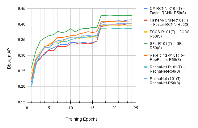
Figure 3: Training process visualization of all experimented detectors.

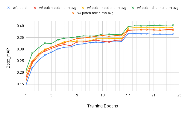
Figure 4: The effect of patch on different dimensions. This experiment is conducted on the RetinaNet-X101-RetinaNet-R50 pair

Appendix E CKA curve in training.

To qualitatively analyze the proposed method, we visualize the CKA similarities in the training phase. As shown in Fig. 5, we can find the CKA values increase with training, which demonstrates that our method does narrow the gap of teacher-student models at the logit level.

Table 11: Ablation study of loss weight $\gamma$.

T$\rightarrow$S	RetinaNet-X101$\rightarrow$RetinaNet-R50
Loss Weight	AP	AP50	AP75	APS	APM	APL
Teacher	41.0	60.9	44.0	23.9	45.2	54.0
Student	37.4	56.7	39.6	20.0	40.7	49.7
$\gamma=5$	39.8	59.4	42.5	22.3	43.5	53.9
$\gamma=10$	40.3	59.9	43.0	23.3	44.2	54.9
$\gamma=15$	38.5	58.0	41.0	20.7	41.8	51.3

Table 12: Ablation study of Batchsize. Noted that ”4 $\times$ 1” means 4 GPUs, each batchsize is 1, totally batchsize is $4\times 1=4$

T$\rightarrow$S	RetinaNet-X101$\rightarrow$RetinaNet-R50
	AP	AP50	AP75	APS	APM	APL
Teacher	41.0	60.9	44.0	23.9	45.2	54.0
Student	37.4	56.7	39.6	20.0	40.7	49.7
Batchsize 4$\times$1	39.9	59.5	42.8	21.7	43.9	53.3
Batchsize 4$\times$2	40.3	59.8	43.1	22.5	44.2	54.4
Batchsize 4$\times$3	40.3	59.9	43.0	23.3	44.2	54.9
Batchsize 4$\times$4	40.0	59.8	42.6	22.9	43.8	54.1

Table 13: Ablation study of number of distillation layers. Noted that ”Layer=1” means choosing 1 layer to distill.

T$\rightarrow$S	RetinaNet-X101$\rightarrow$RetinaNet-R50
	AP	AP50	AP75	APS	APM	APL
Teacher	41.0	60.9	44.0	23.9	45.2	54.0
Student	37.4	56.7	39.6	20.0	40.7	49.7
Layer=1	39.9	59.7	42.8	21.9	43.5	54.1
Layer=2	40.2	59.9	42.6	21.9	44.0	54.6
Layer=3	40.3	59.9	43.0	23.3	44.2	54.9

Table 14: Results on the CIFAR-100 test set. We apply PCKA to the classification task, and it also outforms some of the previous methods.

Distillation Type	Teacher	ResNet110	ResNet110	WRN-40-2 Zagoruyko and Komodakis [2016b]	VGG13
		74.31	74.31	75.61	74.64
	Student	ResNet20 He et al. [2016]	ResNet32	WRN-16-2	VGG8
		69.06	71.14	73.26	72.50
	FitNet Romero et al. [2014]	68.99	71.06	73.58	71.02
	ATKD Zagoruyko and Komodakis [2016a]	70.22	70.55	74.08	71.43
	SPKD Tung and Mori [2019]	70.04	72.69	73.83	72.68
	CCKD Peng et al. [2019]	69.48	71.48	73.56	70.71
	RKD Park et al. [2019]	69.25	71.82	73.35	71.48
	VID Ahn et al. [2019]	70.16	70.38	74.11	71.23
	KD Hinton et al. [2015]	70.67	73.08	74.92	73.33
	DKD Zhao et al. [2022]	-	74.11	76.24	76.32
	DIST Huang et al. [2022]	69.94	73.55	75.29	75.79
	PCKA(ours)	70.97	74.11	75.61	74.98

Appendix F PCKA in image classification

We apply PCKA to the classification task, and it also outperforms well on the methods with the same distillation type, as shown in Table 14. However, PCKA performs very badly on the teacher and student pairs with different architectures. The possible reason is that the cutting activations of different architectures contain more dissimilar and harmful representations, causing difficulty in transferring knowledge to the student.

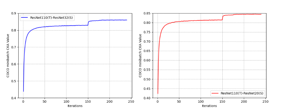
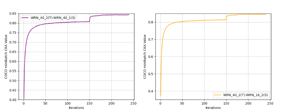
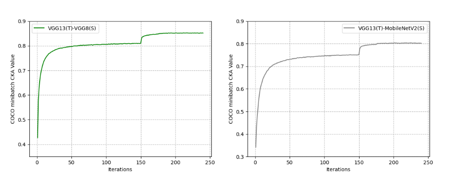
Figure 5: CKA curve in training phase on CIFAR-100. We visualize the CKA similarities in the training for six teacher-student pairs.

References

- Ahn et al. [2019] Sungsoo Ahn, Shell Xu Hu, et al. Variational information distillation for knowledge transfer. In CVPR, pages 9163–9171, Long Beach, CA, USA, Jun. 2019. IEEE.
- Boudiaf et al. [2020] Malik Boudiaf, Jérôme Rony, Imtiaz Masud Ziko, Eric Granger, Marco Pedersoli, Pablo Piantanida, and Ismail Ben Ayed. A unifying mutual information view of metric learning: Cross-entropy vs. pairwise losses. In ECCV, 2020.
- Cai and Vasconcelos [2017] Zhaowei Cai and Nuno Vasconcelos. Cascade r-cnn: Delving into high quality object detection. CVPR, pages 6154–6162, 2017.
- Chen and Wang [2019] Kai Chen and Jiaqi Wang. MMDetection: Open mmlab detection toolbox and benchmark. arXiv preprint arXiv:1906.07155, 2019.
- Chen et al. [2021] Pengguang Chen, Shu Liu, et al. Distilling knowledge via knowledge review. In CVPR, pages 5008–5017, Virtual Event, Jun. 2021. IEEE.
- Chen et al. [2022] Huanran Chen, Shitong Shao, Ziyi Wang, Zirui Shang, Jin Chen, Xiaofeng Ji, and Xinxiao Wu. Bootstrap generalization ability from loss landscape perspective. In European Conference on Computer Vision, pages 500–517. Springer, 2022.
- Chen et al. [2023] Huanran Chen, Yinpeng Dong, Zhengyi Wang, Xiao Yang, Chengqi Duan, Hang Su, and Jun Zhu. Robust classification via a single diffusion model. arXiv preprint arXiv:2305.15241, 2023.
- Chong et al. [2022] Zhiyu Chong, Xinzhu Ma, Hong Zhang, Yuxin Yue, Haojie Li, Zhihui Wang, and Wanli Ouyang. Monodistill: Learning spatial features for monocular 3d object detection. ArXiv, abs/2201.10830, 2022.
- Contributors [2021] MMRazor Contributors. Openmmlab model compression toolbox and benchmark, 2021.
- Cui et al. [2023] Jiequan Cui, Zhuotao Tian, Zhisheng Zhong, Xiaojuan Qi, Bei Yu, and Hanwang Zhang. Decoupled kullback-leibler divergence loss. ArXiv, abs/2305.13948, 2023.
- Dai et al. [2021] Xing Dai, Zeren Jiang, et al. General instance distillation for object detection. In CVPR, pages 7842–7851, Virtual Event, Jun. 2021.
- de Rijk et al. [2022] Philip de Rijk, Lukas Schneider, Marius Cordts, and Dariu M. Gavrila. Structural knowledge distillation for object detection. ArXiv, abs/2211.13133, 2022.
- Frankle and Carbin [2019] Jonathan Frankle and Michael Carbin. The lottery ticket hypothesis: Finding sparse, trainable neural networks. In ICLR, New Orleans, LA, USA, May 2019.
- Gong et al. [2023] Linrui Gong, Shaohui Lin, Baochang Zhang, Yunhang Shen, Ke Li, Ruizhi Qiao, Bohan Ren, Muqing Li, Zhou Yu, and Lizhuang Ma. Adaptive hierarchy-branch fusion for online knowledge distillation. In AAAI, 2023.
- He et al. [2016] Kaiming He, Xiangyu Zhang, et al. Deep residual learning for image recognition. In CVPR, pages 770–778, Las Vegas, NV, USA, Jun. 2016. IEEE.
- Heo et al. [2019] Byeongho Heo, Jeesoo Kim, and Sangdoo et al. A comprehensive overhaul of feature distillation. In ICCV, pages 1921–1930, Seoul, Korea (South), Oct.-Nov. 2019. IEEE.
- Hinton et al. [2015] Geoffrey Hinton, Oriol Vinyals, Jeff Dean, et al. Distilling the knowledge in a neural network. arXiv preprint arXiv:1503.02531, 2(7), 2015.
- Huang et al. [2022] Tao Huang, Shan You, et al. Knowledge distillation from a stronger teacher. In NeurIPS, New Orleans, LA, USA, Nov.-Dec. 2022. NIPS.
- Kornblith et al. [2019] Simon Kornblith, Mohammad Norouzi, Honglak Lee, and Geoffrey E. Hinton. Similarity of neural network representations revisited. ArXiv, abs/1905.00414, 2019.
- Krizhevsky and Hinton [2009] Alex Krizhevsky and Geoffrey Hinton. Learning multiple layers of features from tiny images. Handbook of Sys temic Autoimmune Diseases, 2009.
- Li et al. [2020] Xiang Li, Wenhai Wang, Lijun Wu, Shuo Chen, Xiaolin Hu, Jun Li, Jinhui Tang, and Jian Yang. Generalized focal loss: Learning qualified and distributed bounding boxes for dense object detection. ArXiv, abs/2006.04388, 2020.
- Lin et al. [2014] Tsung-Yi Lin, Michael Maire, et al. Microsoft coco: Common objects in context. In ECCV, pages 740–755, Zurich, Switzerland, Sept. 2014. Springer.
- Lin et al. [2017] Tsung-Yi Lin, Priya Goyal, Ross B. Girshick, Kaiming He, and Piotr Dollár. Focal loss for dense object detection. ICCV, pages 2999–3007, 2017.
- Liu et al. [2021a] Li Liu, Qingle Huang, Sihao Lin, Hongwei Xie, Bing Wang, Xiaojun Chang, and Xiao-Xue Liang. Exploring inter-channel correlation for diversity-preserved knowledge distillation. ICCV, pages 8251–8260, 2021.
- Liu et al. [2021b] Songhua Liu, Tianwei Lin, Dongliang He, Fu Li, Ruifeng Deng, Xin Li, Errui Ding, and Hao Wang. Paint transformer: Feed forward neural painting with stroke prediction. In ICCV, pages 6598–6607, October 2021.
- Marcel and Rodriguez [2010] Sébastien Marcel and Yann Rodriguez. Torchvision the machine-vision package of torch. In ACM MM, pages 1485–1488, Firenze, Italy, Oct. 2010. ACM.
- Nguyen et al. [2020] Thao Nguyen, Maithra Raghu, and Simon Kornblith. Do wide and deep networks learn the same things? uncovering how neural network representations vary with width and depth. ArXiv, abs/2010.15327, 2020.
- Orhan and Pitkow [2017] Emin Orhan and Xaq Pitkow. Skip connections eliminate singularities. In ICLR, 2017.
- Park et al. [2019] Wonpyo Park, Dongju Kim, et al. Relational knowledge distillation. In CVPR, pages 3967–3976, Long Beach, CA, USA, Jun. 2019. IEEE.
- Peng et al. [2019] Baoyun Peng, Xiao Jin, et al. Correlation congruence for knowledge distillation. In ICCV, pages 5007–5016, 2019.
- Qiu et al. [2022] Zengyu Qiu, Xinzhu Ma, Kunlin Yang, Chunya Liu, Jun Hou, Shuai Yi, and Wanli Ouyang. Better teacher better student: Dynamic prior knowledge for knowledge distillation. ArXiv, abs/2206.06067, 2022.
- Ren et al. [2015] Shaoqing Ren, Kaiming He, Ross B. Girshick, and Jian Sun. Faster r-cnn: Towards real-time object detection with region proposal networks. IEEE PAMI, 39:1137–1149, 2015.
- Romero et al. [2014] Adriana Romero, Nicolas Ballas, et al. Fitnets: Hints for thin deep nets. arXiv preprint arXiv:1412.6550, 2014.
- Russakovsky et al. [2015] Olga Russakovsky, Jia Deng, et al. Imagenet large scale visual recognition challenge. IJCV, 115(3):211–252, 2015.
- Saha et al. [2022] Aninda Saha, Alina Bialkowski, and Sara Khalifa. Distilling representational similarity using centered kernel alignment (cka). In BMVC, 2022.
- Shao et al. [2023a] Shitong Shao, Huanran Chen, Zhen Huang, Linrui Gong, Shuai Wang, and Xinxiao Wu. Teaching what you should teach: a data-based distillation method. In Proceedings of the Thirty-Second International Joint Conference on Artificial Intelligence, pages 1351–1359, 2023.
- Shao et al. [2023b] Shitong Shao, Xu Dai, Shouyi Yin, Lujun Li, Huanran Chen, and Yang Hu. Catch-up distillation: You only need to train once for accelerating sampling. arXiv preprint arXiv:2305.10769, 2023.
- Shu et al. [2021] Changyong Shu, Yifan Liu, et al. Channel-wise knowledge distillation for dense prediction. In ICCV, pages 5311–5320, Montreal, Canada, Oct. 2021. IEEE.
- Tian et al. [2019] Zhi Tian, Chunhua Shen, Hao Chen, and Tong He. Fcos: Fully convolutional one-stage object detection. ICCV, pages 9626–9635, 2019.
- Tian et al. [2020] Yonglong Tian, Dilip Krishnan, and Phillip Isola. Contrastive representation distillation. In ICLR, Addis Ababa, Ethiopia, Apr. 2020. OpenReview.net.
- Touvron et al. [2020] Hugo Touvron, Matthieu Cord, Matthijs Douze, Francisco Massa, Alexandre Sablayrolles, and Herv’e J’egou. Training data-efficient image transformers & distillation through attention. In ICML, 2020.
- Tung and Mori [2019] Frederick Tung and Greg Mori. Similarity-preserving knowledge distillation. In ICCV, pages 1365–1374, Seoul, Korea (South), Oct-Nov. 2019. IEEE.
- Wan et al. [2020] Alvin Wan, Xiaoliang Dai, Peizhao Zhang, Zijian He, Yuandong Tian, Saining Xie, Bichen Wu, Matthew Yu, Tao Xu, Kan Chen, Péter Vajda, and Joseph Gonzalez. Fbnetv2: Differentiable neural architecture search for spatial and channel dimensions. CVPR, pages 12962–12971, 2020.
- Wang et al. [2019] Tao Wang, Li Yuan, Xiaopeng Zhang, and Jiashi Feng. Distilling object detectors with fine-grained feature imitation. CVPR, pages 4928–4937, 2019.
- Wu et al. [2016] Jiaxiang Wu, Cong Leng, Yuhang Wang, Qinghao Hu, and Jian Cheng. Quantized convolutional neural networks for mobile devices. In CVPR, Las Vegas, NV, USA, Jun. 2016. IEEE.
- Yang et al. [2019] Ze Yang, Shaohui Liu, Han Hu, Liwei Wang, and Stephen Lin. Reppoints: Point set representation for object detection. ICCV, pages 9656–9665, 2019.
- Yang et al. [2021] Jing Yang, Brais Martinez, et al. Knowledge distillation via softmax regression representation learning. In ICLR. OpenReview.net, 2021.
- Yang et al. [2022a] Zhendong Yang, Zhe Li, et al. Focal and global knowledge distillation for detectors. In CVPR, pages 4643–4652, New Orleans, LA, USA, Jun. 2022. IEEE.
- Yang et al. [2022b] Zhendong Yang, Zhe Li, Mingqi Shao, Dachuan Shi, Zehuan Yuan, and Chun Yuan. Masked generative distillation. In ECCV, 2022.
- Yang et al. [2022c] Zhendong Yang, Zhe Li, Ailing Zeng, Zexian Li, Chun Yuan, and Yu Li. Vitkd: Practical guidelines for vit feature knowledge distillation. ArXiv, abs/2209.02432, 2022.
- Yang et al. [2023] Zhendong Yang, Ailing Zeng, Zhe Li, Tianke Zhang, Chun Yuan, and Yu Li. From knowledge distillation to self-knowledge distillation: A unified approach with normalized loss and customized soft labels. ArXiv, abs/2303.13005, 2023.
- Zagoruyko and Komodakis [2016a] Sergey Zagoruyko and Nikos Komodakis. Paying more attention to attention: Improving the performance of convolutional neural networks via attention transfer. In ICLR, 2016.
- Zagoruyko and Komodakis [2016b] Sergey Zagoruyko and Nikos Komodakis. Wide residual networks. In BMVC, pages 1–15, York, UK, Sept. 2016. BMVA.
- Zhang and Ma [2021] Linfeng Zhang and Kaisheng Ma. Improve object detection with feature-based knowledge distillation: Towards accurate and efficient detectors. In ICLR, pages 1–14. OpenReview.net, 2021.
- Zhao et al. [2022] Borui Zhao, Quan Cui, Renjie Song, Yiyu Qiu, and Jiajun Liang. Decoupled knowledge distillation. In CVPR, pages 11953–11962, New Orleans, LA, USA, Jun. 2022. IEEE.
- Zhixing et al. [2021] Du Zhixing, Rui Zhang, Ming Chang, Shaoli Liu, Tianshi Chen, Yunji Chen, et al. Distilling object detectors with feature richness. NeurIPS, 34:5213–5224, Dec. 2021.
- Zhou and Chen [2023] Zikai Zhou and Huanran Chen. Afn: Adaptive fusion normalization via an encoder-decoder framework. In ArXiv preprint, 2023.