MInD: Improving Multimodal Sentiment Analysis via
Multimodal Information Disentanglement

Abstract

Learning effective joint representations has been a central task in multimodal sentiment analysis. Previous methods focus on leveraging the correlations between different modalities and enhancing performance through sophisticated fusion techniques. However, challenges still exist due to the inherent heterogeneity of distinct modalities, which may lead to distributional gap, impeding the full exploitation of inter-modal information and resulting in redundancy and impurity in the information extracted from features. To address this problem, we introduce the Multimodal Information Disentanglement (MInD) approach. MInD decomposes the multimodal inputs into a modality-invariant component, a modality-specific component, and a remnant noise component for each modality through a shared encoder and multiple private encoders. The shared encoder aims to explore the shared information and commonality across modalities, while the private encoders are deployed to capture the distinctive information and characteristic features. These representations thus furnish a comprehensive perspective of the multimodal data, facilitating the fusion process instrumental for subsequent prediction task. Furthermore, MInD improves the learned representations by explicitly modeling the task-irrelevant noise in an adversarial manner. Experimental evaluations conducted on benchmark datasets, including CMU-MOSI, CMU-MOSEI, and UR-Funny, demonstrate MInD’s superior performance over existing state-of-the-art methods in both multimodal emotion recognition and multimodal humor detection tasks. Codes can be found at https://github.com/WeeeicheN/MInD

1 INTRODUCTION

Recently, there has been a growing interest in Multimodal Sentiment Analysis (MSA). The comprehension of sentiment is often enhanced by cross-modal input, such as visual, audio, and textual information. Consequently, researchers have focused on developing effective joint representations that integrate all relevant information from the collected data [1], while most of the models rely on designing sophisticated fusion techniques [2] for the exploration of the intra-modal and inter-modal dynamics. Although multimodal learning has been theoretically shown to outperform unimodal learning [3], in practice, the modality gap resulting from the inherent heterogeneity of distinct modalities hampers the full exploitation of the inter-modal information for effective multimodal representations. This phenomenon persists across a broad range of multi-modal models, covering texts, natural images, videos, medical images, and amino-acid sequences [4]. Therefore, prior approaches that address the representations of each modality through a comprehensive learning framework may lead to insufficiently refined and potentially redundant multimodal representations.

Recent studies have initiated an exploration into the learning of distinct multimodal representations. Pham et al. [5] translates a source modality to a target modality for joint representations using cyclic reconstruction. Mai et al. [6] also provides a adversarial encoder-decoder classifier framework to learn a modality-invariant embedding space through translating the distributions. But these methods do not explicitly learn the modality-specific representations which reveal the unique characteristic of emotions from different perspectives. By adopting the shared-private learning frameworks [7], Hazarika et al. [8] and Yang et al. [9] attempt to incorporate a diverse set of information by learning different factorized subspaces for each modality in order to obtain better representations for fusion. However, their approaches either utilizes simple constraints that fail to guarantee a perfect factorization, or relies on a complex fusion module which indicates that the extracted information may be unrefined. Moreover, they both neglect the control in the information flow, which could result in the loss of practical information.

Motivated by the above observations, we propose the Multimodal Information Disentanglement (MInD) approach to deal with the insufficient exploitation of information from heterogeneous modalities. The main strategy is to decompose features into three distinct components for each modality with information optimization. Specifically, the first component is the modality-invariant component, which can effectively capture the underlying commonalities and explore the shared information across modalities. Secondly, we train the modality-specific component to capture the distinctive information and characteristic features. Furthermore, as unknown noises in each signal may be categorized as complementary information, we explicitly model the noise component to enhance the refinement of the learned information and mitigate the impact of noise on the quality of the representations. The combination of these three components thus provides a comprehensive view of the given input.

The contributions of this paper can be summarized as:

• We propose MInD, a disentanglement-based multimodal sentiment analysis method driven by information optimization. MInD overcomes the challenge caused by modality heterogeneity via learning modality-invariant, modality-specific and noise representations, thus aiding fusion for prediction tasks.

• We explicity model the noise components to give a more holistic view of the multimodal inputs, as well as improve the quality of learned representations. To the best of our knowledge, we are the first work to introduce the noise components into disentanglement.

• MInD outperforms previous state-of-the-art methods on three standard multimodal benchmarks only with a simple fusion strategy, which demonstrates the power of MInD in capturing diverse facets of multimodal information.

2 RELATED WORKS

2.1 Multimodal Sentiment Analysis

Learning effective joint representations is a critical challenge in MSA. Many previous works have contributed to sophisticated fusion techniques which leverage the correlations between different modalities. Zadeh et al. [2] proposed tensor-based fusion network which applies outer product to model the unimodal, bimodal and trimodal interactions. Mai et al. [6] introduced graph fusion network which regards each interaction as a vertex and the corresponding similarities as weights of edges. Besides, the attention mechanisms [10] are widely used to identify important information [11, 12, 13]. For instance, Shenoy and Sardana [11] assigns weights to the importance differences between multiple modalities through the importance attention network. However, as multimodal inputs have various characteristics and information properties, this inherent heterogeneity of different modalities complicates the analysis of data, thus leading to a significant challenge on the mining and integration of information and the learning of multimodal joint embeddings.

2.2 Disentanglement Learning

Disentanglement learning [7, 14] is designed to unravel complex data structures, isolating key components to extract desirable information for more insightful and efficient data processing. Therefore, this approach plays a pivotal role in aligning semantically related concepts across different modalities and effectively alleviates the problems caused by the modality gap. Furthermore, disentanglement learning significantly contributes to multimodal fusion by offering a more structured and explicit representation [8]. Such clarity and organization in the data representation are instrumental in enhancing the efficacy and precision of multimodal integration processes. For this reason, following Salzmann et al. [15], many works have extended the shared-private learning strategies in various scenarios for excellent results, including retrieval [16], user representation in social network [17], and emotion recognition [9], etc. In comparison, to the best of our knowledge, we provide the first attempt that broaden the shared-private disentangled paradigm to the shared-private-noise disentanglement method.

3 METHOD

3.1 Model Overview

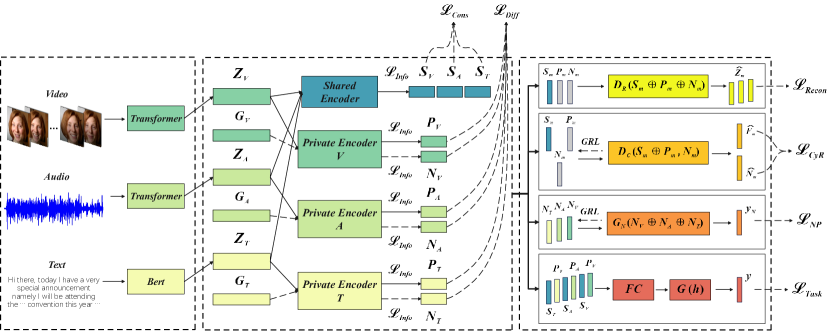
Figure 1: Model Overview.

The overall framework of MInD is shown in Fig. 1. We introduce our method within the context of a task scenario that incorporates three distinct modalities, namely visual, audio, and text. Each individual data point consists of three sequences of low-level features originating from the visual, acoustic, and textual modalities. We denote them as ${\bf X_{V}}\in\mathbf{R}^{L_{V}\times d_{V}}$, ${\bf X_{A}}\in\mathbf{R}^{L_{A}\times d_{A}}$, ${\bf X_{T}}\in\mathbf{R}^{L_{T}\times d_{T}}$, respectively, where $L_{(\cdot)}$ is the sequence length and $d_{(\cdot)}$ is the embedding dimension.

In response to the challenges posed by modality heterogeneity, we aim to identify an approach that effectively mitigates the distributional discrepancy and enhances the efficacy of information extraction, ensuring a comprehensive and nuanced analysis of multimodal inputs. To this end, we decompose the inputs into three parts: a modality-invariant component, a modality-specific component, and a noise component. Note that each noise component of different modalities is generated from gaussian noise, and subsequently sent to the corresponding private encoder. This decomposition is then facilitated through the implementation of information constraints, consistency constraints, and difference constraints. The integration of these constraints helps maximal utilization of information embedded within the high-level feature, enabling efficient exploration of both cross-modal commonality and distinctive features. After that, we evaluate the completeness of decomposed information through a reconstruction module. Moreover, we employ a cyclic reconstruction module to further reduce information redundancy, and a noise prediction module to efficiently minimize the task-related information within the noise components. The modality-invariant components and the modality-specific components are finally fused for prediction tasks.

3.2 Feature Extraction

Here we employ transformer-based models [10] to extract high-level semantic features from individual modalities. Specifically, we use the Bert [18] model for text modality, and we employ a standard transformer model for the remaining two modalities,

$$Z_{m}=F^{m}(X_{m};{\theta}_{m}),\quad m\in\{V,A,T\}.$$ (1)

The refined features of each modality are in a fixed dimension as $Z_{m}\in\mathbf{R}^{d_{k}}$.

3.3 Representation Learning

3.3.1 Modality-Invariant and -Specific Components

While temporal model-based feature extractors effectively capture the long-range contextual dependencies presented in multimodal sequences, they fail to effectively handle feature redundancy due to the divergence of different modalities [19]. Furthermore, the efficacy of the divide-and-conquer processing pattern is affected by the inherent heterogeneity among different modalities.

Inspired by these observations, we employ the shared and private encoders to learn the modality-invariant components and the modality-specific components, which are designed to capture commonality and specificity of individual modalities, respectively. We denote the shared encoder as $E_{S}(\cdot;{\theta}_{S})$, and the private encoders as $E_{P_{m}}(\cdot;{\theta}_{P_{m}})$, where $m\in\{V,A,T\}$. Then the representations are formulated as below:

$$S_{V}=E_{S}(Z_{V};{\theta}_{S}),S_{A}=E_{S}(Z_{A};{\theta}_{S}),S_{T}=E_{S}(Z_{T};{\theta}_{S}),$$ (2)

$$P_{V}=E_{P_{V}}(Z_{V};{\theta}_{P_{V}}),P_{A}=E_{P_{A}}(Z_{A};{\theta}_{P_{A}}),P_{T}=E_{P_{T}}(Z_{T};{\theta}_{P_{T}}),$$ (3)

with $S_{m},P_{m}\in\mathbf{R}^{d_{k}}$. The shared encoder $E_{S}(\cdot;{\theta}_{S})$ shares the parameters ${\theta}_{S}$ across all modalities, while the private encoders $E_{P_{m}}(\cdot;{\theta}_{P_{m}})$ assign separate parameters ${\theta}_{P_{m}}$ for each modality. Both the shared encoder and private encoders are implemented as simple linear network with the activation function of GeLU [20].

3.3.2 Noise Components

While the integration of modality-invariant and modality-specific components facilitates a comprehensive representation of multimodal inputs, we argue that the approach has not yet reached its full potential. The main problem lies in the persistence of noise information within the desired representations, thereby compromising their purity and limiting the model’s expressive capacity. To this end, we generate gaussian noise vectors which are subsequently trained using the same private encoders, namely:

$$G_{m}\sim\mathcal{N}(0,1),\quad N_{m}=E_{P_{m}}(G_{m};{\theta}_{P_{m}}),$$ (4)

where $m\in\{V,A,T\}$. During the procedure, the private encoders are forced to be noise-resistant with the ability to distinguish between the distinctive information and noise information. This strengthens the robustness of the learned representations and aids in the extraction of more refined, purer information.

3.3.3 Information Constraint

A conventional approach to discover useful representations involves maximizing the mutual information (MI) between the input and output of models. However, MI is notoriously difficult to compute, especially in continuous and high-dimensional contexts. A recent solution, known as Deep InfoMax (DIM) [21], facilitates efficient calculation of MI when dealing with high-dimensional input/output pairs from deep neural networks. Therefore, we leverage the global mutual information constraint draw from DIM here. This constraint serves the purpose of estimating and maximizing the MI between input data and learned high-level representations simultaneously. Specifically, we employ the objective function based on the Jensen-Shannon divergence due to its proven stability, aligning with our primary aim of maximizing MI rather than obtaining an precise value. The estimator is shown below:

$$\mathcal{\hat{I}}_{\omega,\theta}^{(JSD)}(Z;E_{\theta}(Z))= E_{\mathcal{P}(Z,E_{\theta}(Z))}[-sp(-T_{\omega}(Z,E_{\theta}(Z)))]$$

$$- E_{\mathcal{P}(Z)\times\mathcal{P}(E_{\theta}(Z))}[sp(T_{\omega}(Z,E_{\theta}(Z)))],$$ (5)

where $E_{\theta}(Z)$ is the encoder parameterized by $\theta$, $\mathcal{P}(\cdot)$ is the empirical probability distribution, $sp(\mathit{z})=log(1+e^{\mathit{z}})$ is the softplus function, and $T_{\omega}:\mathcal{X}\times\mathcal{Y}\rightarrow\mathbf{R}$ is a discriminator function modeled by a neural network with parameters $\omega$ called the statistics network.

Since the modality-invariant components are expected to capture cross-modal commonality, we calculate the MI between the outputs and the combination of inputs. Besides, to encourage the noise components to retain less useful information, we also maximize the MI between the noise components and the generated gaussian noise inputs. We denote the above procedure as following:

$$\mathcal{L}_{Info}= \frac{1}{3}\sum_{m\in\{V,A,T\}}-\mathcal{\hat{I}}_{\omega_{S},\theta_{S}}^{(JSD)}(Z_{V}\oplus Z_{A}\oplus Z_{T};S_{m})$$

$$+ \frac{1}{3}\sum_{m\in\{V,A,T\}}-\mathcal{\hat{I}}_{\omega_{P_{m}},\theta_{P_{m}}}^{(JSD)}(Z_{m};P_{m})$$

$$+ \frac{1}{3}\sum_{m\in\{V,A,T\}}-\mathcal{\hat{I}}_{\omega_{P_{m}},\theta_{P_{m}}}^{(JSD)}(G_{m};N_{m})$$ (6)

3.3.4 Consistency Constraint

Inspired by  [22], we introduce the Barlow Twins loss (BT loss) to be the consistency constraint. BT loss is originally designed for learning embeddings which are invariant to distortions of the input sample, it forces two embedding vectors to be similar by making the cross-correlation matrix as close to the identity matrix as possible, which minimizes the redundancy between the components of these vectors. Concretely, each representation pair $S^{A},S^{B}$ is normalized to be mean-centered along the batch dimension as $S^{A,nor},S^{B,nor}$, such that each unit has mean output 0 over the batch. The normalized matrices can be then utilized to depict the cross-correlation matrix:

$$\mathcal{C}_{ij}^{A,B}=\frac{\sum_{b}s_{b,i}^{A,nor}s_{b,j}^{B,nor}}{\sqrt{\sum_{b}(s_{b,i}^{A,nor})^{2}}\sqrt{\sum_{b}(s_{b,j}^{B,nor})^{2}}},$$ (7)

where $b$ indexes batch samples and $i,j$ index the vector dimension of the networks’ outputs. The BT loss is expressed as:

$$\mathcal{L}_{BT}^{m_{1},m_{2}}=\sum_{i}(1-\mathcal{C}_{ii}^{m_{1},m_{2}})^{2}+\lambda_{BT}\sum_{i}\sum_{j\neq i}(\mathcal{C}_{ij}^{m_{1},m_{2}})^{2}.$$ (8)

In the purpose of exploring shared information and commonality across modalities, we transfer the concept into our case by treating different modalities as different views. Following the observations in  [23], we set $\lambda_{BT}$ to be the dimension of the embeddings, and calculate the BT loss between the modality-invariant components of each modalities pair:

$$\mathcal{L}_{Cons}=\frac{1}{3}\sum_{(m_{1},m_{2})}\mathcal{L}_{BT}^{m_{1},m_{2}}$$ (9)

3.3.5 Difference Constraint

Since both the modality-invariant components and the modality-specific components are learned from the same high-level features $Z_{m}$, it may result in the redundancy of information. Moreover, the modality-specific components and the noise components from the same private encoders should be effectively distinguished too. To ensure these three components can model different aspects of multimodal data, we employ the Hilbert-Schmidt Independence Criterion (HSIC) [24] to effectively measure the independence. Formally, the HSIC constraint between any two representations $R_{1},R_{2}$ is defined as:

$$HSIC(R_{1},R_{2})=(n-1)^{-2}\textit{Tr}(UK_{1}UK_{2}),$$ (10)

where $K_{1}$ and $K_{2}$ are the Gram matrices with $k_{1,ij}=k_{1}(r_{1}^{i},r_{1}^{j})$ and $k_{2,ij}=k_{1}(r_{1}^{i},r_{1}^{j})$. And $U=I-(1/n)ee^{T}$, where $I$ is an identity matrix and $e$ is an all-one column vector. In our setting, we use the inner product kernel function for $K_{1}$ and $K_{2}$. To augment the distinction among individual components, the overall difference constraint is expressed as:

$$\mathcal{L}_{Diff}=\frac{1}{12}\sum_{(R_{1},R_{2})}HSIC(R_{1},R_{2}),$$ (11)

where $(R_{1},R_{2})$ is the pair from $(S_{m},P_{m})$, $(S_{m},N_{m})$, $(P_{m_{1}},P_{m_{2}})$, and $(P_{m},N_{m})$.

3.3.6 Reconstruction Constraint

To ensure the completeness of learned information within the decomposed components, we add a reconstruction constraint, which aims to help the combination of representations capture more comprehensive information of their respective modality. By employing a decoder function $\hat{Z}_{m}=D_{R}(S_{m}\oplus P_{m}\oplus N_{m})$. the reconstruction constraint is then designed as the mean squared error between $Z_{m}$ and $\hat{Z}_{m}$:

$$\mathcal{L}_{Recon}=\frac{1}{3}\sum_{m\in\{V,A,T\}}\frac{\|Z_{m}-\hat{Z}_{m}\|_{2}^{2}}{d_{k}},$$ (12)

where $\|\cdot\|_{2}^{2}$ is the squared $L_{2}$-norm.

3.4 Noise Modeling

Although we explicitly incoporate a noise components in our model and enhance the independence between different components through difference constraints, this may still be insufficient alone to improve the quality of the representations. The main reason is that the modality-invariant and -specific information can still propagate through the noise vectors. Therefore, we employ an additional method to directly minimize the MI between the noise components and the other parts. However, the minimization of MI between two vectors presents a significant challenge, owing to the absence of an explicit upper bound that can be directly optimized. To this end, we minimize the MI using DiCyR [25], which leverages cyclic-reconstruction and gradient-reversal layers [26] to force the modality-invariant and -specific components share little mutual information with the noise components. Let $F_{m}$ be the concatenation of $S_{m}$ and $P_{m}$, and $D_{C}(\cdot;\theta_{F_{m}})$, $D_{C}(\cdot;\theta_{N_{m}})$ be the decoders for reconstruction from $F_{m}$ to $N_{m}$ and from $N_{m}$ to $F_{m}$, respectively. The objective is then formulated as below:

$$\mathcal{L}_{CyR}= \frac{1}{6}\sum_{m\in\{V,A,T\}}\|F_{m}-D_{C}(GRL(N_{m});\theta_{N_{m}})\|_{2}^{2}$$

$$+ \frac{1}{6}\sum_{m\in\{V,A,T\}}\|N_{m}-D_{C}(GRL(F_{m});\theta_{F_{m}})\|_{2}^{2},$$ (13)

where $GRL(\cdot)$ is a gradient reversal layer.

3.5 Task Prediction

Until now, the information disentanglement has been conducted in the unsupervised manner. We now complete our final objective function with the downstream task. The learned modality-invariant and -specific components are first fused by a simple linear layer with dimension reduction, and subsequently trained via shallow MLPs $G(\cdot;\theta_{G})$ with several hidden layers and GeLU activation to get the prediction denoted as $\{\hat{y}_{i}\}$ or $\hat{Y}$:

$$h=FC(S_{V}\oplus S_{A}\oplus S_{T}\oplus P_{V}\oplus P_{A}\oplus P_{T})$$ (14)

$$\hat{Y}=G(h)$$ (15)

Specifically, to further reduce the task-related information being propagated into the noise components, we devise a noise-prediction loss with another shallow MLPs $G_{N}(\cdot;\theta_{G_{N}})$, for the prediction $\{\hat{y}_{N,i}\}$ or $\hat{Y}_{N}$ from noise:

$$\hat{Y}_{N}=G_{N}(GRL(N_{V}\oplus N_{A}\oplus N_{T});\theta_{G_{N}})$$ (16)

$$\mathcal{L}_{NP}=-\frac{1}{n}\sum_{i=1}^{n}y_{i}\cdot log\hat{y}_{N,i}\quad or\quad\frac{1}{n}\|Y_{i}-\hat{Y}_{N,i}\|_{2}^{2}.$$ (17)

The final objective function is computed as:

$$\mathcal{L}_{all}= \mathcal{L}_{Task}+\omega\mathcal{L}_{NP}$$

$$+ \alpha\mathcal{L}_{Info}+\beta\mathcal{L}_{Cons}+\gamma\mathcal{L}_{Diff}+\lambda\mathcal{L}_{Recon}+\eta\mathcal{L}_{CyR},$$ (18)

Here, $\alpha,\beta,\gamma,\lambda,\eta,\omega$ determine the contribution of each constraint to the overall loss. And $\mathcal{L}_{Task}$ is the prediction loss, where we employ the standard cross-entropy loss for the classification task, and the mean error loss for the regression task.

Dataset	CMU-MOSI	CMU-MOSEI	UR-FUNNY
$\alpha$	$1e^{-2}$	$2e^{-2}$	$1e^{-2}$
$\beta$	$1e^{-4}$	$2e^{-4}$	$1e^{-4}$
$\gamma$	$1e^{-3}$	$1e^{-3}$	$1e^{-4}$
$\lambda$	$1e^{-1}$	1	$1e^{-1}$
$\eta$	$1e^{-1}$	1	$1e^{-2}$
$\omega$	1	1	$8e^{-3}$

Table 1: Loss coefficients setting in our experiments.

Models	CMU-MOSI					CMU-MOSEI					UR-FUNNY
	Acc7$\uparrow$	Acc2$\uparrow$	F1$\uparrow$	MAE$\downarrow$	Corr$\uparrow$	Acc7$\uparrow$	Acc2$\uparrow$	F1$\uparrow$	MAE$\downarrow$	Corr$\uparrow$	Acc2$\uparrow$
TFN	34.9	80.8	80.7	0.901	0.698	50.2	82.5	82.1	0.593	0.700	68.57
LMF	33.2	82.5	82.4	0.917	0.695	48.0	82.0	82.1	0.623	0.677	67.53
MFM	35.4	81.7	81.6	0.877	0.706	51.3	84.4	84.3	0.568	0.717	-
ICCN	39.0	83.0	83.0	0.862	0.714	51.6	84.2	84.2	0.565	0.713	-
MulT	40.0	83.0	82.8	0.871	0.698	51.8	82.5	82.3	0.580	0.703	-
MISA	42.3	83.4	83.6	0.783	0.761	52.2	85.5	85.3	0.555	0.756	70.61
Self-MM	-	85.9	85.9	0.713	0.798	-	85.1	85.3	0.530	0.765	-
BBFN	45.0	84.3	84.3	0.776	0.755	54.8	86.2	86.1	0.529	0.767	71.68
FDMER	44.1	84.6	84.7	0.724	0.788	54.1	86.1	85.8	0.536	0.773	71.87
CubeMLP	45.5	85.6	85.5	0.770	0.767	54.9	85.1	84.5	0.529	0.760	-
AcFormer	44.2	85.4	85.2	0.715	0.794	54.7	86.5	85.8	0.531	0.786	-
MInD(ours)	45.8	86.0	86.0	0.705	0.796	53.9	86.6	86.7	0.529	0.772	72.43

Table 2: Performance compared with the SOTA approaches in CMU-MOSI, CMU-MOSEI and UR-FUNNY. Top-3 results are marked, with the best in bold and the second to third underlined. According to the comparison, MInD outperforms all approaches.

Models	CMU-MOSI		CMU-MOSEI		UR-FUNNY
	MAE$\downarrow$	Corr$\uparrow$	MAE$\downarrow$	Corr$\uparrow$	Acc2$\uparrow$
MInD	0.705	0.796	0.529	0.772	72.43
Role of Modality
w/o visual	0.722	0.790	0.541	0.770	69.85
w/o Audio	0.736	0.780	0.547	0.764	70.18
w/o Text	1.505	0.123	0.841	0.209	49.67
Role of Disentanglement
w/o M-Invariant	0.801	0.773	0.546	0.767	70.58
w/o M-Specific	0.760	0.779	0.550	0.772	70.46
w/o Noise	0.827	0.775	0.534	0.766	71.64
Non-Disentangled	0.872	0.756	0.537	0.774	71.64
Role of Constraint
w/o $\mathcal{L}_{Info}$	0.780	0.758	0.542	0.761	71.34
w/o $\mathcal{L}_{Cons}$	0.822	0.782	0.537	0.768	71.73
w/o $\mathcal{L}_{Diff}$	0.755	0.788	0.535	0.770	71.70
w/o $\mathcal{L}_{Recon}$	0.723	0.780	0.558	0.758	71.09
w/o $\mathcal{L}_{CyR}$	0.821	0.785	0.539	0.763	71.55
w/o $\mathcal{L}_{NP}$	0.764	0.782	0.532	0.771	71.95
Only $\mathcal{L}_{Task}$	0.837	0.757	0.546	0.768	71.16

Table 3: Results of ablation studies.

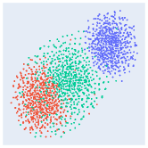
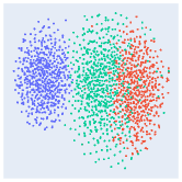
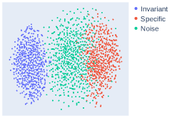
(a) Distribution before training for visual, audio, and text modality from left to right.

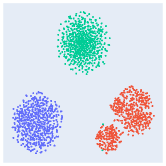
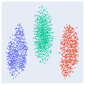
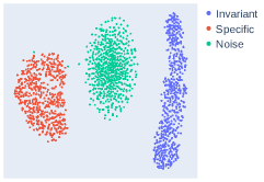
(b) Distribution after training for visual, audio, and text modality from left to right.

Figure 2: Visualization results of the components from distinct modalities in the testing set of CMU-MOSI.

4 EXPERIMENTS

4.1 Datasets and evaluation criteria

In this paper, we choose three multi-modal dataset for evaluation, namely CMU-MOSI and CMU-MOSEI for emotion recognition, and UR-FUNNY for humor detection.

CMU-MOSI  [27] is a widely-utilized dataset for MSA. The dataset is collected from 2199 opinion video clips from YouTube, which is splited to 1284 samples for training set, 229 samples for validation set, and 686 samples for testing set, with sentiment score ranges from -3 to 3 for each sample. Same as previous works, we adopt the 7-class accuracy (Acc-7), the binary accuracy (Acc-2), mean absolute error (MAE), the Pearson Correlation (Corr), and the F1 score for evaluation.

CMU-MOSEI  [28] is a similar but larger dataset that contains 22,856 movie review video clips from YouTube, including 16,326 training samples, 1,871 validation samples, and 4,659 testing samples. Each sample also has a sentiment scores ranging from -3 to 3. The same metrics are employed as in the above setting.

UR-FUNNY  [29] dataset contains 16,514 samples of multimodal punchlines labeled with a binary label for humor/non-humor instance from TED talks, which is partitioned into 10,598 samples in the training set, 2,626 in the validation set, and 3,290 in the testing set. We report the binary accuracy (Acc-2) for this binary classification task.

4.2 Implementation Details

4.2.1 Feature Extraction

Following recent works, we utilize the pretrained BERT-base-uncased model to obtain a 768-dimension embedding for textual features. Specifically, since the original transcripts are not available for our considered UR-FUNNY version, we follow the same procedure as  [8] to retrieve the raw texts from Glove [30]. The acoustic features are extracted from COVAREP [31], where the dimensions are 74 for MOSI/MOSEI and 81 for UR-FUNNY. Moreover, we use Facet to extract facial expression features for both MOSI and MOSEI, and OpenFace [32] for UR-FUNNY. The final visual feature dimensions are 47 for MOSI, 35 for MOSEI, and 75 for UR-FUNNY.

4.3 Experimental Setup

All models are built on the Pytorch 2.0.1 with one single Nvidia 3090 GPU. The number of transformer encoder layers for visual and audio are both 3. For the MOSI, MOSEI and UR-FUNNY benchmarks, the batch sizes and epochs are {32,32,32} and {100,100,100}, respectively. The Adam optimizer is adopted for network optimization with an initial learning rate of $\{3e^{-5},2e^{-5},2e^{-5}\}$. The hidden dimension $d_{k}$ is set to {512,256,256}, and the output dimension of fusion vector $h$ is 128 for all datasets. The loss coefficient is listed in Table 1.

4.4 Comparison With SOTA Models

Baselines.

We compare our model with many baselines, including pure learning based models such as TFN  [2], LMF  [33], MFM  [34], and MulT  [35]. Besides, we also compare our model with feature space manipulation approaches like ICCN  [36], MISA  [8], Self-MM  [37], BBFN  [38], and FDMER  [9]. Moreover, the more recent and competitive methods CubeMLP  [39] and AcFormer (word-aligned version)  [40] are also taken into our consideration. All the models are compared under word-aligned setting.

Multimodal Emotion Recognition.

As shown in Table 2, MInD outperforms all baselines on most evaluation metrics on both MOSI and MOSEI. Specifically, on the MOSI dataset, our approach show the best results on Acc-7, Acc-2, MAE, and the F1 score, with only a 0.002 decrease for the Corr compared to SOTA. While on the MOSEI dataset, MInd enhances the highest Acc-2 and the F1 score by 0.1 (for AcFormer) and 0.6 (for BBFN), respectively. Although the performance of our approach on the Corr ranks the third on MOSEI, MInd obtains a relatively lower Acc-7 than that in SOTA. This is understandable since MInd only adopt simple concatenation and lower linear layers for fusion and prediction, which limit fine-grained sentiment calculation on larger dataset. However, we still achieve overall satisfactory results without sophisticated fusion strategy, which reveals that our approach is able to capture sufficiently distinct information to form a comprehensive view of multimodal inputs. Note that, all the baselines exhibit an inability to maintain their performance relative to other models when the dataset changes. On the contrary, MInD consistently demonstrates robust performance despite of the alteration of data, which shows the superiority of our approach. In addition, compared to the MISA and FDMER which both utilize disentanglement-based methods, MInD shows consistent and notable improvement on both dataset. This is attributed to our introduction of noise components that efficiently enhances the robustness of the learned representations and aids in the extraction of more refined, purer information.

Multimodal Humor Detection.

Further experiments are conducted on the UR-FUNNY dataset to verify the applicability of MInD in Table 2. Since humor detection is sensitive to heterogeneous representations of different modalities, the best result achieved by MInD demonstrate the efficacy of our proposed multimodal framework in learning distinct representations and capturing reliable information.

4.5 Ablation Studies

Role of Modality.

In Table 3, we remove each modality separately to explore the performance of the bi-modal MInD, which performs consistently worse compared to the tri-modal MInD, suggesting that distinct modalities provides indispensable information. Specifically, we observe a significant drop in performance when we remove the text modality, yet similar drops are not observed in the other two cases. This shows the dominance of the text modality over the visual and audio modalities, probably due to the reason that the text modality contains manual transcriptions which could be inherently better, while on the contrary, the visual and audio modalities contain unfiltered raw signals with more noisy and redundant information.

Role of Disentanglement.

To empirically validate the effectiveness of the proposed modality-invariant component, the modality-specific component and the noise component, we exclude each component separately for evaluation. As shown in Table 3, the worse performance indicates that each component captures different aspect of the information and is hence essential and meaningful. We also find that the noise component plays a more important role in the smaller dataset MOSI, where we observe the worst results without it rather than other components. As models trained on less samples are more susceptible to noise, this observation underscores the significance of our explicit noise modeling strategy in enhancing the robustness of learned features for small datasets. In addition, we provide a non-disentangled version where the extracted features from the transformer-based models are directly utilized for fusion and prediction, of which the even worse results on MOSI further demonstrate the robustness of our model. For the MOSEI and UR-FUNNY, due to the learning limitations in a partial subspace, the non-disentangled model is slightly better compared to those incorporating only a subset of components.

Role of Constraint.

We further verify the essentiality of all the constraints in our model through the results in Table 3. When there is no $\mathcal{L}_{Info}$, information extracted from the high-level features may be insufficient due to the simple structure of the common and private encoders. This in turn demonstrates that with the help of well designed constraints, neural network models can be simple but effective. When we remove $\mathcal{L}_{Cons}$ or $\mathcal{L}_{Diff}$, model fails to capture the shared information or specific information of distinct modalities, which obtains slightly better results than that in the non-disentangled version. As $\mathcal{L}_{Recon}$ and $\mathcal{L}_{CyR}$ either ensure the completeness or refinement of learned information, removing them also brings worse performance. The removal of $\mathcal{L}_{NP}$ leads to a least drop in MOSEI and UR-FUNNY, and it is worth noting that the result on UR-FUNNY in this case still surpasses the baselines, indicating the significance of the combination of other constraints. Finally, we present the results trained only with $\mathcal{L}_{Task}$, the largest performance decrease in MAE and Acc-2 together demonstrate the necessity of all the constraints in our model.

4.6 Visualization of Decomposed Components

To further demonstrate that MInD actually reduces the information redundancy and depicts different aspects of information. we visualize the feature distributions of each component of distinct modalities before and after training. The visualization is conducted by using T-SNE [41] with samples from the testing set of the CMU-MOSI dataset. It can be seen that before training, representations from different components are clustered closely in the feature space, while the modality-specific components and the noise components are even distributed without clear boundary since they are produced from the same private encoders. Instead, after training, the representations from individual components become more separated in the feature space, and the distributional discrepancy shows that our method effectively reduces the overlapping of information, which guarantees a better exploitation of useful information.

5 CONCLUSION

In this paper, we propose the Multimodal Information Disentanglement (MInD) method to overcome the challenges caused by the inherent heterogeneity of distinct modalities through the decomposition of multimodal inputs into modality-invariant, modality-specific and noise components. We obtain the refined representations via the well-designed constraints and improve the quality of disentanglement with the help of explicitly modeling the noise, which provides a new insight to look into the noise during the learning of different representation subspaces. Experimental results demonstrate the superiority of our method. In the future, we plan to broaden the applicative spectrum of our method, deploying it across a diverse array of multimodal scenarios.

References

- [1] Soujanya Poria, Devamanyu Hazarika, Navonil Majumder, and Rada Mihalcea. Beneath the tip of the iceberg: Current challenges and new directions in sentiment analysis research. IEEE Transactions on Affective Computing, 2020.
- [2] Amir Zadeh, Minghai Chen, Soujanya Poria, Erik Cambria, and Louis-Philippe Morency. Tensor fusion network for multimodal sentiment analysis. arXiv preprint arXiv:1707.07250, 2017.
- [3] Yu Huang, Chenzhuang Du, Zihui Xue, Xuanyao Chen, Hang Zhao, and Longbo Huang. What makes multi-modal learning better than single (provably). Advances in Neural Information Processing Systems, 34:10944–10956, 2021.
- [4] Victor Weixin Liang, Yuhui Zhang, Yongchan Kwon, Serena Yeung, and James Y Zou. Mind the gap: Understanding the modality gap in multi-modal contrastive representation learning. Advances in Neural Information Processing Systems, 35:17612–17625, 2022.
- [5] Hai Pham, Paul Pu Liang, Thomas Manzini, Louis-Philippe Morency, and Barnabás Póczos. Found in translation: Learning robust joint representations by cyclic translations between modalities. In Proceedings of the AAAI Conference on Artificial Intelligence, volume 33, pages 6892–6899, 2019.
- [6] Sijie Mai, Haifeng Hu, and Songlong Xing. Modality to modality translation: An adversarial representation learning and graph fusion network for multimodal fusion. In Proceedings of the AAAI Conference on Artificial Intelligence, volume 34, pages 164–172, 2020.
- [7] Konstantinos Bousmalis, George Trigeorgis, Nathan Silberman, Dilip Krishnan, and Dumitru Erhan. Domain separation networks. Advances in neural information processing systems, 29, 2016.
- [8] Devamanyu Hazarika, Roger Zimmermann, and Soujanya Poria. Misa: Modality-invariant and-specific representations for multimodal sentiment analysis. In Proceedings of the 28th ACM international conference on multimedia, pages 1122–1131, 2020.
- [9] Dingkang Yang, Shuai Huang, Haopeng Kuang, Yangtao Du, and Lihua Zhang. Disentangled representation learning for multimodal emotion recognition. In Proceedings of the 30th ACM International Conference on Multimedia, pages 1642–1651, 2022.
- [10] Ashish Vaswani, Noam Shazeer, Niki Parmar, Jakob Uszkoreit, Llion Jones, Aidan N Gomez, Łukasz Kaiser, and Illia Polosukhin. Attention is all you need. Advances in neural information processing systems, 30, 2017.
- [11] Aman Shenoy and Ashish Sardana. Multilogue-net: A context aware rnn for multi-modal emotion detection and sentiment analysis in conversation. arXiv preprint arXiv:2002.08267, 2020.
- [12] Md Shad Akhtar, Dushyant Singh Chauhan, Deepanway Ghosal, Soujanya Poria, Asif Ekbal, and Pushpak Bhattacharyya. Multi-task learning for multi-modal emotion recognition and sentiment analysis. arXiv preprint arXiv:1905.05812, 2019.
- [13] Jiasen Lu, Jianwei Yang, Dhruv Batra, and Devi Parikh. Hierarchical question-image co-attention for visual question answering. Advances in neural information processing systems, 29, 2016.
- [14] Hyunjik Kim and Andriy Mnih. Disentangling by factorising. In International Conference on Machine Learning, pages 2649–2658. PMLR, 2018.
- [15] Mathieu Salzmann, Carl Henrik Ek, Raquel Urtasun, and Trevor Darrell. Factorized orthogonal latent spaces. In Proceedings of the thirteenth international conference on artificial intelligence and statistics, pages 701–708. JMLR Workshop and Conference Proceedings, 2010.
- [16] Weikuo Guo, Huaibo Huang, Xiangwei Kong, and Ran He. Learning disentangled representation for cross-modal retrieval with deep mutual information estimation. In Proceedings of the 27th ACM International Conference on Multimedia, pages 1712–1720, 2019.
- [17] Wenyi Tang, Bei Hui, Ling Tian, Guangchun Luo, Zaobo He, and Zhipeng Cai. Learning disentangled user representation with multi-view information fusion on social networks. Information Fusion, 74:77–86, 2021.
- [18] Jacob Devlin, Ming-Wei Chang, Kenton Lee, and Kristina Toutanova. Bert: Pre-training of deep bidirectional transformers for language understanding. arXiv preprint arXiv:1810.04805, 2018.
- [19] Yi Zhang, Mingyuan Chen, Jundong Shen, and Chongjun Wang. Tailor versatile multi-modal learning for multi-label emotion recognition. In Proceedings of the AAAI Conference on Artificial Intelligence, volume 36, pages 9100–9108, 2022.
- [20] Dan Hendrycks and Kevin Gimpel. Gaussian error linear units (gelus). arXiv preprint arXiv:1606.08415, 2016.
- [21] R Devon Hjelm, Alex Fedorov, Samuel Lavoie-Marchildon, Karan Grewal, Phil Bachman, Adam Trischler, and Yoshua Bengio. Learning deep representations by mutual information estimation and maximization. arXiv preprint arXiv:1808.06670, 2018.
- [22] Jure Zbontar, Li Jing, Ishan Misra, Yann LeCun, and Stéphane Deny. Barlow twins: Self-supervised learning via redundancy reduction. In International Conference on Machine Learning, pages 12310–12320. PMLR, 2021.
- [23] Yao-Hung Hubert Tsai, Shaojie Bai, Louis-Philippe Morency, and Ruslan Salakhutdinov. A note on connecting barlow twins with negative-sample-free contrastive learning. arXiv preprint arXiv:2104.13712, 2021.
- [24] Le Song, Alex Smola, Arthur Gretton, Karsten M Borgwardt, and Justin Bedo. Supervised feature selection via dependence estimation. In Proceedings of the 24th international conference on Machine learning, pages 823–830, 2007.
- [25] David Bertoin and Emmanuel Rachelson. Disentanglement by cyclic reconstruction. IEEE Transactions on Neural Networks and Learning Systems, 2022.
- [26] Yaroslav Ganin, Evgeniya Ustinova, Hana Ajakan, Pascal Germain, Hugo Larochelle, François Laviolette, Mario March, and Victor Lempitsky. Domain-adversarial training of neural networks. Journal of machine learning research, 17(59):1–35, 2016.
- [27] Amir Zadeh, Rowan Zellers, Eli Pincus, and Louis-Philippe Morency. Multimodal sentiment intensity analysis in videos: Facial gestures and verbal messages. IEEE Intelligent Systems, 31(6):82–88, 2016.
- [28] AmirAli Bagher Zadeh, Paul Pu Liang, Soujanya Poria, Erik Cambria, and Louis-Philippe Morency. Multimodal language analysis in the wild: Cmu-mosei dataset and interpretable dynamic fusion graph. In Proceedings of the 56th Annual Meeting of the Association for Computational Linguistics (Volume 1: Long Papers), pages 2236–2246, 2018.
- [29] Md Kamrul Hasan, Wasifur Rahman, Amir Zadeh, Jianyuan Zhong, Md Iftekhar Tanveer, Louis-Philippe Morency, et al. Ur-funny: A multimodal language dataset for understanding humor. arXiv preprint arXiv:1904.06618, 2019.
- [30] Jeffrey Pennington, Richard Socher, and Christopher D Manning. Glove: Global vectors for word representation. In Proceedings of the 2014 conference on empirical methods in natural language processing (EMNLP), pages 1532–1543, 2014.
- [31] Gilles Degottex, John Kane, Thomas Drugman, Tuomo Raitio, and Stefan Scherer. Covarep—a collaborative voice analysis repository for speech technologies. In 2014 ieee international conference on acoustics, speech and signal processing (icassp), pages 960–964. IEEE, 2014.
- [32] Tadas Baltrušaitis, Peter Robinson, and Louis-Philippe Morency. Openface: an open source facial behavior analysis toolkit. In 2016 IEEE winter conference on applications of computer vision (WACV), pages 1–10. IEEE, 2016.
- [33] Zhun Liu, Ying Shen, Varun Bharadhwaj Lakshminarasimhan, Paul Pu Liang, Amir Zadeh, and Louis-Philippe Morency. Efficient low-rank multimodal fusion with modality-specific factors. arXiv preprint arXiv:1806.00064, 2018.
- [34] Yao-Hung Hubert Tsai, Paul Pu Liang, Amir Zadeh, Louis-Philippe Morency, and Ruslan Salakhutdinov. Learning factorized multimodal representations. arXiv preprint arXiv:1806.06176, 2018.
- [35] Yao-Hung Hubert Tsai, Shaojie Bai, Paul Pu Liang, J Zico Kolter, Louis-Philippe Morency, and Ruslan Salakhutdinov. Multimodal transformer for unaligned multimodal language sequences. In Proceedings of the conference. Association for Computational Linguistics. Meeting, volume 2019, page 6558. NIH Public Access, 2019.
- [36] Zhongkai Sun, Prathusha Sarma, William Sethares, and Yingyu Liang. Learning relationships between text, audio, and video via deep canonical correlation for multimodal language analysis. In Proceedings of the AAAI Conference on Artificial Intelligence, volume 34, pages 8992–8999, 2020.
- [37] Wenmeng Yu, Hua Xu, Ziqi Yuan, and Jiele Wu. Learning modality-specific representations with self-supervised multi-task learning for multimodal sentiment analysis. In Proceedings of the AAAI conference on artificial intelligence, volume 35, pages 10790–10797, 2021.
- [38] Wei Han, Hui Chen, Alexander Gelbukh, Amir Zadeh, Louis-philippe Morency, and Soujanya Poria. Bi-bimodal modality fusion for correlation-controlled multimodal sentiment analysis. In Proceedings of the 2021 International Conference on Multimodal Interaction, pages 6–15, 2021.
- [39] Hao Sun, Hongyi Wang, Jiaqing Liu, Yen-Wei Chen, and Lanfen Lin. Cubemlp: An mlp-based model for multimodal sentiment analysis and depression estimation. In Proceedings of the 30th ACM International Conference on Multimedia, pages 3722–3729, 2022.
- [40] Daoming Zong, Chaoyue Ding, Baoxiang Li, Jiakui Li, Ken Zheng, and Qunyan Zhou. Acformer: An aligned and compact transformer for multimodal sentiment analysis. In Proceedings of the 31st ACM International Conference on Multimedia, pages 833–842, 2023.
- [41] Laurens Van der Maaten and Geoffrey Hinton. Visualizing data using t-sne. Journal of machine learning research, 9(11), 2008.