Regression Copulas for Multivariate Responses

We propose a novel distributional regression model for a multivariate response vector based on a copula process over the covariate space. It uses the implicit copula of a Gaussian multivariate regression, which we call a “regression copula”. To allow for large covariate vectors their coefficients are regularized using a novel multivariate extension of the horseshoe prior. Bayesian inference and distributional predictions are evaluated using efficient variational inference methods, allowing application to large datasets. An advantage of the approach is that the marginal distributions of the response vector can be estimated separately and accurately, resulting in predictive distributions that are marginally-calibrated. Two substantive applications of the methodology highlight its efficacy in multivariate modeling. The first is the econometric modeling and prediction of half-hourly regional Australian electricity prices. Here, our approach produces more accurate distributional forecasts than leading benchmark methods. The second is the evaluation of multivariate posteriors in likelihood-free inference (LFI) of a model for tree species abundance data, extending a previous univariate regression copula LFI method. In both applications, we demonstrate that our new approach exhibits a desirable marginal calibration property.

Keywords: Copula Process; Distributional Regression; Implicit Copula; Likelihood-Free Inference; Semiparametric Multivariate Regression; Variational Inference

1 Introduction

Distributional regression, which extends traditional mean based regression models to allow the entire distribution to be a function of a covariate vector, is increasingly popular. For a univariate response, there are many approaches including (but not restricted to) GAMLSS models (Rigby and Stasinopoulos, 2005), conditional transformation models (Hothorn et al., 2014), mixtures of experts models (Jordan and Jacobs, 1994), quantile regression (Koenker and Bassett, 1978) and regression copula models (Klein and Smith, 2019; Smith and Klein, 2021). However, effective distributional regression methods for a multivariate response vector are much more limited. In this paper we extend the regression copula model to the multivariate case, and demonstrate its advantages in two challenging applications, one from econometric modeling and another from likelihood free inference in ecology.

Klein and Smith (2019) combine a copula process over the covariate space with an arbitrary marginal for a univariate response to define a distributional regression. Distributional predictions are given by the Bayesian predictive distribution from the copula model. The copula used is the implicit copula of the response values (called pseudo responses hereafter) from a Bayesian regularized Gaussian regression model with its regression coefficients marginalized out. The authors call this a “regression copula” because it is a function of the covariates, a term that we also employ here. To extend this approach we construct an implicit copula from a Bayesian multivariate regularized Gaussian regression model with the regression coefficients marginalized out. This presents a number of challenges. First, an effective regularization prior is required for the regression coefficients, and for this we propose a novel multivariate extension of the horseshoe prior (Carvalho et al., 2009; Carvalho and Polson, 2010). This conjugate prior is scaled by the correlation matrix of the regression disturbance in the same way as the g-priors of Brown et al. (1998) and Smith and Kohn (2000). We show that the marginal priors for the regression coefficients of each equation in the multivariate regression are standard horseshoe priors. The second challenge is the selection of a prior for the cross-equation correlation matrix, and we consider two choices. The first is an order-invariant prior suggested by Archakov and Hansen (2021), and the second is based on a factor model as proposed by Murray et al. (2013) and allows application of our model to high-dimensional response vectors.

A third challenge is that, unlike Klein and Smith (2019) who use MCMC to evaluate the posterior of their univariate distributional regression, application of MCMC is difficult here because the posterior is both more complex and of a much higher dimension. Therefore, we use an efficient variational inference (VI) method with a parsimonious Gaussian approximation and stochastic gradient optimization methods that employ efficient reparameterized gradients (Ong et al., 2018). This is faster and more robust than MCMC. A final challenge is that the joint posterior is computationally intractable. Therefore we propose using an augmented posterior density that is fast to compute as the the target of our variational optimization. The end result is a method that can be employed with large datasets in high dimensions and with sizeable covariate vectors.

A major advantage of our method is that the user has complete control over the choice of marginal distribution for each response variable. Moreover, the predictive distributions are marginally-calibrated, which is where their long run average matches this marginal (Gneiting et al., 2007). These advantages, and the efficacy of our approach, are shown in two demanding applications. The first is the modeling and forecasting of intraday Australian regional electricity prices using a large dataset. Here, we show that our approach can account for the complex non-Gaussian distributions of electricity prices, the nonlinear effect of regional demands on each regional price, and the strong inter-regional dependence in prices. In an extensive forecasting study we show that the marginally-calibrated distributional forecasts are more accurate than a range of benchmark methods.

The second application is to likelihood-free inference (LFI) of an ecological model of tree species abundance census data. In LFI, distributional regression methods can be used to approximate the posterior distribution when the likelihood is intractable or inference is based only on summary statistics. In this ecological example our multivariate distributional regression method extends a previous univariate LFI regression copula approach by approximating the full joint posterior distribution while maintaining a desirable marginal calibration property. An analysis of tree species abundance fluctuations also demonstrates the benefits of using LFI methods to deal with model misspecification through summary statistic based inference.

The rest of the paper is organized as follows. Section 2 shows how to specify a copula process model for distributional regression. Section 3 specifies the implicit copula of the pseudo responses from a regularized multivariate regression. This is a Bayesian formulation using carefully constructed priors. Section 4 describes the VI method for estimation and distributional prediction, while Section 5 contains the econometric application. Section 6 applies our distributional regression to multivariate posterior estimation in LFI for the ecological model, while Section 7 concludes.

2 Copula Model for Multivariate Regression

We first outline a regression model for a vector-valued response $\bm{Y}_{i}=(Y_{i,1},\ldots,Y_{i,p})^{\top}$ that is based on a copula process. It is a distributional regression model, which is where the entire predictive distribution of $\bm{Y}_{i}$ is a function of a covariate vector $\text{\boldmath$x$}_{i}=(x_{i,1},\ldots,x_{i,q})^{\top}$. The employed copula process will be defined in Section 3.

2.1 Copula process model

Denote $n$ realizations on each continuous-valued dependent variable as $\bm{Y}_{1:n,j}=(Y_{1,j},\ldots,Y_{n,j})^{\top}$ for $j=1,\ldots,p$, and corresponding covariate vectors $\text{\boldmath$x$}_{1:n}=\{\text{\boldmath$x$}_{1},\ldots,\text{\boldmath$x$}_{n}\}$ that are common across response components $j$. Then, we define the distribution of $\bm{Y}_{1:n}=(\bm{Y}_{1:n,1}^{\top},\ldots,\bm{Y}_{1:n,p}^{\top})^{\top}$ (that is, the dependent variables stacked first by realization and then by variable), conditional on $\text{\boldmath$x$}_{1:n}$, using a copula model with distribution function

$$F_{Y_{1:n}}(\text{\boldmath$y$}_{1:n}|\text{\boldmath$x$}_{1:n},\text{\boldmath$\vartheta$})=C_{1:n}\left(\text{\boldmath$u$}_{1:n,1}^{\top},\ldots,\text{\boldmath$u$}_{1:n,p}^{\top};\text{\boldmath$x$}_{1:n},\text{\boldmath$\vartheta$}\right)\,,\;\mbox{ for }n\geq 2\,,\;p\geq 1.$$ (1)

Here, $C_{1:n}$ is a copula function on the unit cube $[0,1]^{np}$ with uniform margins. The arguments of the copula function are $\text{\boldmath$u$}_{1:n,j}^{\top}=(u_{1,j},\ldots,u_{n,j})$ with $u_{i,j}=F_{Y_{i,j}}(y_{i,j}|\text{\boldmath$x$}_{i})$, where $F_{Y_{i,j}}$ is the cumulative distribution function of $Y_{i,j}|\text{\boldmath$x$}_{i}$, which is the margin of $F_{Y_{1:n}}$. In this paper the copula is a function of $\text{\boldmath$x$}_{1:n}$ with parameters $\vartheta$ that do not vary with $n$, so that it is a “copula process” (Wilson and Ghahramani, 2010) on the covariate space.

If $\text{\boldmath$u$}_{1:n}=(\text{\boldmath$u$}_{1:n,1}^{\top},\ldots,\text{\boldmath$u$}_{1:n,p}^{\top})^{\top}$, then differentiating (1) with respect to $y$ gives the density

$$f_{Y_{1:n}}(\text{\boldmath$y$}_{1:n}|\text{\boldmath$x$}_{1:n},\text{\boldmath$\vartheta$})=c_{1:n}\left(\text{\boldmath$u$}_{1:n};\text{\boldmath$x$}_{1:n},\text{\boldmath$\vartheta$}\right)\prod_{i=1}^{n}\prod_{j=1}^{p}f_{Y_{i,j}}(y_{i,j}|\text{\boldmath$x$}_{i})\,,$$ (2)

with $f_{Y_{i,j}}(y|\text{\boldmath$x$}_{i})=\frac{d}{dy}F_{Y_{i,j}}(y|\text{\boldmath$x$}_{i})$ and $c_{1:n}(\text{\boldmath$u$};\text{\boldmath$x$}_{1:n},\text{\boldmath$\vartheta$})=\frac{\partial^{np}}{\partial\text{\boldmath$u$}}C_{1:n}(\text{\boldmath$u$};\text{\boldmath$x$}_{1:n},\text{\boldmath$\vartheta$})$ is commonly called the “copula density”.

One advantage of the model at (1) is that if $F_{Y_{i,j}}=G_{j}$ is assumed invariant with respect to index $i$ and covariates $\text{\boldmath$x$}_{i}$, then the margins $G_{1},\ldots,G_{p}$ can be estimated using nonparametric or other flexible estimators, as we do here. Because the copula $C_{1:n}$ is a function of the covariates $\text{\boldmath$x$}_{1:n}$, Smith and Klein (2021) call such a copula process a “regression copula”. We stress that this model should not be confused with a copula model with marginals that are regressions and a parametric copula that is either independent of the covariates (as in Pitt et al., 2006; Song et al., 2009) or also covariate-dependent (as in Acar et al., 2013).

2.2 Multivariate distributional regression

The copula model at (1) and (2) specifies a distributional multivariate regression model, even when $G_{1},\ldots,G_{p}$ are not functions of $\text{\boldmath$x$}_{i}$. To see why, consider the prediction of a new realization of the response vector $\bm{Y}_{n+1}=(Y_{n+1,1},\ldots,Y_{n+1,p})^{\top}$. The predictive density, conditional on existing observations $\bm{Y}_{1:n}=\bm{y}_{1:n}$, covariates $\text{\boldmath$x$}_{1:n+1}$ and parameters $\vartheta$, is

$$p(\text{\boldmath$y$}_{n+1}|\text{\boldmath$y$}_{1:n},\text{\boldmath$x$}_{1:n+1},\text{\boldmath$\vartheta$}) = \frac{f_{Y_{1:n+1}}(\text{\boldmath$y$}_{1:n+1}|\text{\boldmath$x$}_{1:n+1},\text{\boldmath$\vartheta$})}{f_{Y_{1:n}}(\text{\boldmath$y$}_{1:n}|\text{\boldmath$x$}_{1:n},\text{\boldmath$\vartheta$})}=\frac{c_{1:n+1}(\text{\boldmath$u$}_{1:n+1};\text{\boldmath$x$}_{1:n+1},\text{\boldmath$\vartheta$})}{c_{1:n}(\text{\boldmath$u$}_{1:n+1};\text{\boldmath$x$}_{1:n},\text{\boldmath$\vartheta$})}\prod_{j=1}^{p}g_{j}(y_{n+1,j})$$ (3)

$$= p(\text{\boldmath$u$}_{n+1}|\text{\boldmath$u$}_{1:n},\text{\boldmath$x$}_{1:n+1},\text{\boldmath$\vartheta$})\prod_{j=1}^{p}g_{j}(y_{n+1,j})\,,$$

where the marginal density of $Y_{i,j}$ is $f_{Y_{i,j}}=g_{j}=\frac{dG_{j}}{dy_{j}}$. Thus, the entire predictive density is a function $\text{\boldmath$x$}_{n+1}$ (and also $\text{\boldmath$x$}_{1:n}$) through the first term in (3) that is due to the copula process. A Bayesian method for computing (3) efficiently for the copula process proposed in this paper is outlined in Section 4.3.

3 Implicit Copula Process

The choice of copula at (1) is key to our multivariate response regression model, for which we use an “implicit copula” with parameters $\vartheta$. This is the copula of a parametric multivariate distribution constructed by inversion of Sklar’s theorem. In particular, we use the implicit copula of the distribution of realizations from a Gaussian multivariate regression with the regression coefficients integrated out. The dependent variables of these regressions are called “pseudo” responses because they are unobserved. Our model entails a Bayesian formulation for which we propose a novel extension of the horseshoe prior (Carvalho et al., 2009; Carvalho and Polson, 2010) for the entire vector of regression coefficients.

3.1 Multivariate regression model

Let $\widetilde{\bm{Z}}_{1:n,j}=(\widetilde{Z}_{1,j},\dots,\widetilde{Z}_{n,j})^{\top}$ be a vector of $n$ realizations on a pseudo variable. For each variable $j=1,\ldots,p$, we consider a linear regression with the same $q$ covariates, given by

$$\widetilde{\bm{Z}}_{1:n,j}=F\text{\boldmath$\beta$}_{j}+\text{\boldmath$\epsilon$}_{j}\,,\mbox{ for }j=1,\ldots,p\,,$$ (4)

where $F=\left[\text{\boldmath$x$}_{1}|\cdots|\text{\boldmath$x$}_{n}\right]^{\top}$ is an $n\times q$ design matrix and $\text{\boldmath$\beta$}_{j}=(\beta_{1,j},\dots,\beta_{q,j})^{\top}$ are the coefficients. The regression has Gaussian distributed errors $\text{\boldmath$\epsilon$}_{j}=(\epsilon_{1,j},\ldots,\epsilon_{n,j})^{\top}$ that are correlated across equations but not observations, with $E(\epsilon_{i,j}\epsilon_{i^{\prime},l})=\sigma_{j,l}$ if $i=i^{\prime}$, and zero otherwise.

We stack the pseudo-responses and errors in the same order as $\bm{Y}_{1:n}$ in the previous section, so that $\widetilde{\bm{Z}}_{1:n}=(\widetilde{\bm{Z}}_{1:n,1}^{\top},\dots,\widetilde{\bm{Z}}_{1:n,p}^{\top})^{\top}$ and $\text{\boldmath$\epsilon$}=(\text{\boldmath$\epsilon$}_{1}^{\top},\dots,\text{\boldmath$\epsilon$}_{p}^{\top})^{\top}$. Then, if $\text{\boldmath$\beta$}=(\text{\boldmath$\beta$}_{1}^{\top},\dots,\text{\boldmath$\beta$}_{p}^{\top})^{\top}$, and $X=I_{p}\otimes F$ (where $\otimes$ denotes the Kronecker product and $I_{p}$ a $p\times p$ identity matrix), the system of $p$ regressions can be written in stacked form as

$$\widetilde{\bm{Z}}_{1:n}=X\text{\boldmath$\beta$}+\text{\boldmath$\epsilon$}\,,\;\mbox{ with }\text{\boldmath$\epsilon$}|\Sigma\sim N(\bm{0},\Sigma\otimes I_{n})\,,$$ (5)

with $\Sigma=\{\sigma_{j,l}\}_{j=1:p,\,l=1:p}$ a $p\times p$ covariance matrix. This model is the “seemingly unrelated regression” (SUR) of Zellner (1962) with common covariates for each of the $p$ regression equations.

3.2 Extended horseshoe prior

Regularization of $\beta$ is advantageous when either $q$ or $p$ is large, including when $F$ contains function basis terms as in Section 5. This is achieved in a Bayesian analysis through its prior, and here we propose a novel prior for $\beta$ that extends the horseshoe prior to the multivariate response regression case. To specify this prior, we first define two matrix operators as follows. Let bdiag be a matrix operator with $D=\mbox{bdiag}(D_{1},\ldots,D_{p})$ the $pq\times pq$ block diagonal matrix with $q\times q$ blocks $D_{j}$ each of the same dimension. If each block $D_{j}$ is positive definite with upper triangular Cholesky factorization $D_{j}=U_{j}^{\top}U_{j}$, then define the operator “$\star$” so that

$$\Sigma\star D=\{\sigma_{jl}U_{j}^{\top}U_{l}\}_{j=1:p,l=1:p}=U^{\top}(\Sigma\otimes I_{q})U\,,$$

for $U=\mbox{bdiag}(U_{1},\ldots,U_{p})$. With this notation, the conjugate prior we use is

$$\text{\boldmath$\beta$}|\Sigma,\text{\boldmath$\theta$}\sim N\left(\bm{0},\Sigma\star P(\text{\boldmath$\theta$})^{-1}\right)\,,$$ (6)

where $P(\text{\boldmath$\theta$})=\mbox{bdiag}(P_{1}(\text{\boldmath$\theta$}_{1}),\ldots,P_{p}(\text{\boldmath$\theta$}_{p}))$ and $\text{\boldmath$\theta$}=(\text{\boldmath$\theta$}_{1}^{\top},\dots,\text{\boldmath$\theta$}_{p}^{\top})^{\top}$. The matrix $P_{j}(\text{\boldmath$\theta$}_{j})$ is the diagonal precision matrix of a standard horseshoe prior for regression $j$ with hyper-parameters $\text{\boldmath$\theta$}_{j}$, for $j=1,\ldots,p$. Writing the Cholesky factors of $P_{j}^{-1}$ and $P^{-1}$ as $P_{j}^{-1/2}$ and $P^{-1/2}$, respectively, the $pq\times pq$ prior covariance matrix at (6) can be expressed as

$$\Sigma\star P(\text{\boldmath$\theta$})^{-1}=\{\sigma_{jl}P_{j}(\text{\boldmath$\theta$}_{j})^{-1/2}P_{l}(\text{\boldmath$\theta$}_{l})^{-1/2}\}_{j=1:p,l=1:p}=P(\text{\boldmath$\theta$})^{-1/2}(\Sigma\otimes I_{q})P(\text{\boldmath$\theta$})^{-1/2}\,.$$

We make three observations concerning this prior. First, the prior covariance is scaled by $\Sigma$ in the same manner as the $g$-prior for a SUR model given in Brown et al. (1998) and Smith and Kohn (2000). Second, the marginal prior is $\text{\boldmath$\beta$}_{j}|\Sigma,\text{\boldmath$\theta$}\sim N(\bm{0},\sigma_{jj}P_{j}^{-1}(\text{\boldmath$\theta$}_{j}))$, which is a standard horseshoe regularization prior for regression equation $j$ at (4). Third, the prior is a conjugate but dependent prior for $\text{\boldmath$\beta$}_{1},\ldots,\text{\boldmath$\beta$}_{p}$ (e.g. $E(\text{\boldmath$\beta$}_{j}\text{\boldmath$\beta$}_{l}^{\top})=\sigma_{jl}P_{j}(\text{\boldmath$\theta$}_{j})^{-1/2}P_{l}(\text{\boldmath$\theta$}_{l})^{-1/2}$) in contrast to independent horseshoe priors as in Li et al. (2021). Adopting our prior greatly simplifies the expression and computation of the posterior with $\beta$ marginalized out as in Section 3.3 below.

To finalize the regularized regression specification, as in the standard horseshoe prior we specify $P_{j}(\text{\boldmath$\theta$}_{j})^{-1}=\mbox{diag}(\xi_{j,1}^{2},\ldots,\xi_{j,q}^{2})$, with hyper-priors $\xi_{j,k}|\tau_{j}\sim\mbox{Half-Cauchy}(0,\tau_{j})\,,\mbox{ and }\tau_{j}\sim\mbox{Half-Cauchy}(0,1)$. Setting $\text{\boldmath$\theta$}_{j}=(\xi_{j,1},\ldots,\xi_{j,p},\tau_{j})^{\top}$, we assume these hyper-parameters are independent across regressions $j=1,\ldots,p$ a priori.

3.3 Regression copula derivation

Following Klein and Smith (2019) and Smith and Klein (2021) we construct the implicit copula of the distribution of $\widetilde{\bm{Z}}_{1:n}|\text{\boldmath$x$}_{1:n},\Sigma,\text{\boldmath$\theta$}$ with $\beta$ integrated out. (Notice that if $\beta$ was not integrated out, then from (4) the implicit copula of $\widetilde{\bm{Z}}_{1:n}|\text{\boldmath$x$}_{1:n},\Sigma,\text{\boldmath$\beta$},\text{\boldmath$\theta$}$ is simply the independence copula). Recognizing a Gaussian in $\beta$ and applying the Woodbury formula (see Part A.1 of the Web Appendix) gives $\widetilde{\bm{Z}}_{1:n}|\text{\boldmath$x$}_{1:n},\Sigma,\text{\boldmath$\theta$}\sim N(\bm{0},V)$ with

$$V=(\Sigma\otimes I_{n})+X(\Sigma\star P(\text{\boldmath$\theta$})^{-1})X^{\top}\,,$$

In our model $X=(I_{p}\otimes F)$, and with some straightforward matrix algebra, the second term can be simplified further as

$$X(\Sigma\star P(\text{\boldmath$\theta$})^{-1})X^{\top} = (I_{p}\otimes F)(\Sigma\star P(\text{\boldmath$\theta$})^{-1})(I_{p}\otimes F^{\top})$$

$$= \left\{\sigma_{lj}FP_{l}(\text{\boldmath$\theta$}_{l})^{-1/2}P_{j}(\text{\boldmath$\theta$}_{j})^{-1/2}F^{\top}\right\}_{l=1:p,j=1:p}=\widetilde{F}(\Sigma\otimes I_{q})\widetilde{F}^{\top}\,,$$

with $\widetilde{F}=\mbox{bdiag}(FP_{1}(\text{\boldmath$\theta$}_{1})^{-1/2},\cdots,FP_{p}(\text{\boldmath$\theta$}_{p})^{-1/2})$.

Write the diagonal matrix $S=\mbox{diag}(V)^{-1/2}$, then the implicit copula of a Gaussian distribution is a Gaussian copula (Song, 2000) with a parameter matrix given by the correlation matrix $R=SVS$. In Part A.2 of the Web Appendix we establish the following two results. First, $R$ is a function of $\Sigma$ only through the term $\mbox{diag}(\Sigma)^{-1/2}\Sigma\,\mbox{diag}(\Sigma)^{-1/2}$. Therefore, without loss of generality, we set $\sigma_{jj}=1$ for all $j$, so $\Sigma$ is strictly a correlation matrix that is identified in the copula. The second result is that $S=\mbox{bdiag}(S_{1},\ldots,S_{p})$, with

$$S_{j}=\mbox{diag}\left((1+\text{\boldmath$x$}_{1}^{\top}P_{j}(\text{\boldmath$\theta$}_{j})^{-1}\text{\boldmath$x$}_{1})^{-1/2},\ldots,(1+\text{\boldmath$x$}_{n}^{\top}P_{j}(\text{\boldmath$\theta$}_{j})^{-1}\text{\boldmath$x$}_{n})^{-1/2}\right)\,.$$

Hence, $S$ is a diagonal matrix which can be computed in $O(npq)$ operations because evaluating $\text{\boldmath$x$}_{i}^{\top}P_{j}(\text{\boldmath$\theta$}_{j})^{-1}\text{\boldmath$x$}_{i}$ is $O(q)$.

Denoting $R$ as a function of $\{\Sigma,\text{\boldmath$\theta$},\text{\boldmath$x$}_{1:n}\}$, the $np$-dimensional copula density at (2) is the well-known Gaussian copula density given by

$$c_{1:n}(\text{\boldmath$u$}_{1:n};\text{\boldmath$x$}_{1:n},\text{\boldmath$\vartheta$})=\frac{\phi_{np}\left(\text{\boldmath$z$}_{1:n};\bm{0},R(\Sigma,\text{\boldmath$\theta$},\text{\boldmath$x$}_{1:n})\right)}{\prod_{i=1}^{n}\prod_{j=1}^{p}\phi_{1}(z_{i,j})},$$ (7)

where $\text{\boldmath$z$}_{1:n}=(\text{\boldmath$z$}_{1:n,1}^{\top},\dots,\text{\boldmath$z$}_{1:n,p}^{\top})^{\top}$, $\text{\boldmath$z$}_{1:n,j}=(z_{1,j},\dots,z_{n,j})^{\top}$ and $z_{i,j}=\Phi_{1}^{-1}(u_{i,j})$. Here, $\phi_{d}(\cdot;\text{\boldmath$\mu$},\Omega)$ and $\Phi_{d}(\cdot;\text{\boldmath$\mu$},\Omega)$ denote the density and distribution functions of a $N_{d}(\text{\boldmath$\mu$},\Omega)$ distribution, respectively, and we write simply $\phi_{1}(\cdot)$ and $\Phi_{1}(\cdot)$ when $d=1$, $\text{\boldmath$\mu$}=0$ and $\Omega=1$. The copula parameters are $\text{\boldmath$\vartheta$}=\{\Sigma,\text{\boldmath$\theta$}\}$. This is a Gaussian copula process on the covariate space, because the correlation matrix $R$ in (7) is a function of the covariate values $\text{\boldmath$x$}_{1:n}$. When $p=1$ it simplifies to the copula process for a univariate response given in Klein et al. (2021).

The random vector $\bm{Z}_{1:n}=S\widetilde{\bm{Z}}_{1:n}\sim N_{np}(\bm{0},R)$, from which $\text{\boldmath$z$}_{1:n}$ in (7) is a drawn. These are dependent upon $\{\text{\boldmath$x$}_{1:n},\text{\boldmath$\theta$},\Sigma\}$, which is an observation that is important when considering estimation and inference in Section 4.

3.4 Priors for $\Sigma$

There are a range of different parameterizations and priors for correlation matrices (Ghosh et al., 2021). In our model, $\Sigma$ captures cross-sectional dependence, and we employ two priors suitable for this case. The first (labeled “Prior 1”) is based on a re-parameterization of $\Sigma$ to a vector $\text{\boldmath$\upsilon$}\in\mathbb{R}^{p(p-1)/2}$ proposed by Archakov and Hansen (2021). This prior is order invariant, and the elements of $\upsilon$ are on the same scale, which simplifies the selection of a hyperprior for them. The second (labeled “Prior 2”) is based on a factor model as proposed by Murray et al. (2013), which has the advantage that it is scalable with $p$. Appendix A details both priors and the resulting parameters $\vartheta$.

4 Estimation

4.1 Parameter Augmentation

From (2) and (7), the likelihood of our copula model is

$$f_{Y_{1:n}}(\text{\boldmath$y$}_{1:n};\text{\boldmath$x$}_{1:n},\text{\boldmath$\vartheta$})=\phi_{np}\left(\text{\boldmath$z$}_{1:n};\bm{0},R(\Sigma,\text{\boldmath$\theta$},\text{\boldmath$x$}_{1:n})\right)\prod_{i=1}^{n}\prod_{j=1}^{p}\frac{g_{j}(y_{i,j})}{\phi_{1}(z_{i,j})}\,.$$ (8)

However, because $R$ is a dense $n\times n$ matrix, evaluating the likelihood becomes computationally intractable for large $n$. Therefore, we use an augmentation method for posterior computation that avoids evaluating $R$ directly by reintroducing the parameters $\beta$ from the model for the pseudo-responses (5) as follows.

Let $\text{\boldmath$\eta$}=\{\text{\boldmath$\beta$},\text{\boldmath$\vartheta$}\}$ and $J(\text{\boldmath$\vartheta$},\text{\boldmath$x$}_{1:n})=\prod_{i=1}^{n}\prod_{j=1}^{p}\frac{g_{j}(y_{i,j})}{\phi_{1}(z_{i,j})}$ be the term arising from the transformation of variables from $\bm{Y}_{1:n}$ to $\bm{Z}_{1:n}$ . Then we evaluate the augmented posterior

$$p(\text{\boldmath$\eta$}|\text{\boldmath$y$}_{1:n},\text{\boldmath$x$}_{1:n}) \propto p(\text{\boldmath$y$}_{1:n}|\text{\boldmath$x$}_{1:n},\text{\boldmath$\eta$})p(\text{\boldmath$\eta$})$$

$$\propto p(\text{\boldmath$z$}_{1:n}|\text{\boldmath$x$}_{1:n},\text{\boldmath$\beta$},\text{\boldmath$\vartheta$})J(\text{\boldmath$\vartheta$},\text{\boldmath$x$}_{1:n})p(\text{\boldmath$\beta$}|\text{\boldmath$\vartheta$})p(\text{\boldmath$\vartheta$})$$

$$= \phi_{np}(\text{\boldmath$z$}_{1:n};SX\text{\boldmath$\beta$},S(\Sigma\otimes I_{n})S)J(\text{\boldmath$\vartheta$},\text{\boldmath$x$}_{1:n})p(\text{\boldmath$\beta$}|\Sigma,\text{\boldmath$\theta$})p(\text{\boldmath$\vartheta$})\,.$$ (10)

The marginal density in $\vartheta$ of the augmented posterior above is the posterior obtained using the likelihood at (8) and an identical prior. However, evaluating (10) is much faster because it only involves diagonal and block-diagonal matrices with low-dimensional blocks.

4.2 Variational inference

It is difficult to evaluate the complex and high-dimensional augmented posterior at (10) using an MCMC scheme, and we instead employ variational inference (VI) which is typically faster and more robust for such target distributions. Following (Ong et al., 2018), a Gaussian approximation with a covariance matrix that has a parsimonious factor structure is used. The approximating density is $q_{\lambda}(\text{\boldmath$\eta$})=\phi_{T}(\text{\boldmath$\eta$};\text{\boldmath$\mu$},BB^{\top}+\Delta^{2})$, where $T$ denotes the length of $\eta$, $\mu$ is a mean vector, $B$ is a factor loading matrix of dimension $T\times M$ where $M\ll T$ is the number of factors, $\Delta$ is a diagonal matrix with elements $\text{\boldmath$\delta$}=(\delta_{1},\dots,\delta_{T})^{\top}$. The full set of variational parameters are therefore $\text{\boldmath$\lambda$}=(\text{\boldmath$\mu$}^{\top},\text{vec}(B)^{\top},\text{\boldmath$\delta$}^{\top})^{\top}$ with $\text{vec}(B)$ denoting the vectorization of $B$.

At (10), denote the extended likelihood term as $l(\text{\boldmath$\eta$})=p(\text{\boldmath$z$}_{1:n}|\text{\boldmath$x$}_{1:n},\text{\boldmath$\beta$},\text{\boldmath$\vartheta$})J(\text{\boldmath$\vartheta$},\text{\boldmath$x$}_{1:n})$, the prior as $p(\text{\boldmath$\eta$})$, and the augmented posterior up to proportionality as $h(\text{\boldmath$\eta$})=p(\text{\boldmath$\eta$})l(\text{\boldmath$\eta$})$. VI proceeds by optimizing the so-called evidence lower bound ${\cal L}(\text{\boldmath$\lambda$})$, defined as

$${\cal L}(\text{\boldmath$\lambda$}) =E_{q}(\log h(\text{\boldmath$\eta$})-\log q_{\lambda}(\text{\boldmath$\eta$})),$$ (11)

where $E_{q}(\cdot)$ denotes the expectation with respect to $q_{\lambda}(\text{\boldmath$\eta$})$. Maximizing (11) with respect to the variational parameters $\lambda$ is equivalent to minimizing the Kullback-Leibler divergence between $q_{\lambda}(\text{\boldmath$\eta$})$ and the posterior distribution. A common way to perform the optimization is to use stochastic gradient methods, where we initialize with a value $\text{\boldmath$\lambda$}^{(0)}$ and then update this value iteratively as

$$\text{\boldmath$\lambda$}^{(k+1)}=\text{\boldmath$\lambda$}^{(k)}+\text{\boldmath$a$}_{k}\circ\widehat{\nabla_{\text{\boldmath$\lambda$}}{\cal L}(\text{\boldmath$\lambda$}^{(k)})},$$

for $k\geq 0$, where $\widehat{\nabla_{\text{\boldmath$\lambda$}}{\cal L}(\text{\boldmath$\lambda$}^{(k)})}$ is an unbiased estimate of the gradient $\nabla_{\text{\boldmath$\lambda$}}{\cal L}(\text{\boldmath$\lambda$})$ at $\text{\boldmath$\lambda$}=\text{\boldmath$\lambda$}^{(k)}$, $\text{\boldmath$a$}_{k}$ is a $T$-dimensional vector of step sizes at step $k$ and “$\circ$” denotes elementwise multiplication. The recursion above converges to a local mode of ${\cal L}(\text{\boldmath$\lambda$})$ under conditions on the step sizes and other regularity conditions, and updating occurs until some stopping rule is satisfied.

Among the most effective methods for computing low variance unbiased estimate of the gradient is to use so-called reparametrization gradients (Kingma and Welling, 2014; Rezende et al., 2014). A draw from density $q_{\lambda}(\text{\boldmath$\eta$})$ is given by $\text{\boldmath$\eta$}=\text{\boldmath$\mu$}+B\text{\boldmath$w$}_{1}+\text{\boldmath$\delta$}\circ\text{\boldmath$w$}_{2}$, with $\text{\boldmath$w$}=(\text{\boldmath$w$}_{1}^{\top},\text{\boldmath$w$}_{2}^{\top})^{\top}\sim N_{M+T}(\bm{0},I)$. Using this generative representation Ong et al. (2018) show the reparameterization gradient with respect to $\lambda$ is

$$\nabla_{\mu}{\cal L}(\text{\boldmath$\lambda$}) =E(\nabla_{\vartheta}\log h(\text{\boldmath$\mu$}+B\text{\boldmath$w$}_{1}+\text{\boldmath$\delta$}\circ\text{\boldmath$w$}_{2})+(BB^{\top}+\Delta^{2})^{-1}(B\text{\boldmath$w$}_{1}+\text{\boldmath$\delta$}\circ\text{\boldmath$w$}_{2})),$$

$$\nabla_{B}{\cal L}(\text{\boldmath$\lambda$}) =E(\nabla_{\vartheta}\log h(\text{\boldmath$\mu$}+B\text{\boldmath$w$}_{1}+\text{\boldmath$\delta$}\circ\text{\boldmath$w$}_{2})\text{\boldmath$w$}_{1}^{\top}+(BB^{\top}+\Delta^{2})^{-1}(B\text{\boldmath$w$}_{1}+\text{\boldmath$\delta$}\circ\text{\boldmath$w$}_{2})\text{\boldmath$w$}_{1}^{\top}),$$

$$\nabla_{\delta}{\cal L}(\text{\boldmath$\lambda$}) =E(\text{diag}(\nabla_{\vartheta}\log h(\text{\boldmath$\mu$}+B\text{\boldmath$w$}_{1}+\text{\boldmath$\delta$}\circ\text{\boldmath$w$}_{2})\text{\boldmath$w$}_{2}^{\top}+(BB^{\top}+\Delta^{2})^{-1}(B\text{\boldmath$w$}_{1}+\text{\boldmath$\delta$}\circ\text{\boldmath$w$}_{2})\text{\boldmath$w$}_{2}^{\top}))\,,$$

where the expectations above are with respect to the distribution of $w$. The computations involving $(BB^{\top}+\Delta^{2})^{-1}$ are undertaken efficiently using the Woodbury formula, and Monte Carlo estimates of the gradients are obtained using one or more Monte Carlo samples of $w$. Analytical expressions for $\nabla_{\vartheta}\log h(\text{\boldmath$\eta$})$ are derived in Part B of the Web Appendix, which we employ because it is faster and more accurate to evaluate than automatic differentiation.

4.3 Predictive inference

Next, we consider predictive inference for an as yet unobserved response $\bm{Y}_{n+1}$ given corresponding covariates $\text{\boldmath$x$}_{n+1}$. Let $\text{\boldmath$z$}_{n+1}=(z_{n+1,1},\dots,z_{n+1,p})^{\top}$, $z_{n+1,j}=\Phi^{-1}(G_{j}(y_{n+1,j}))$, and $S_{n+1}$ be the diagonal matrix defined in Section 3.3. Then, the predictive density at (3) is

$$p(\text{\boldmath$y$}_{n+1}|\text{\boldmath$x$}_{1:n+1},\text{\boldmath$y$}_{1:n})=E\left(\phi_{p}\left(\text{\boldmath$z$}_{n+1};S_{n+1}(I_{p}\otimes\text{\boldmath$x$}_{n+1})\text{\boldmath$\beta$},S_{n+1}\Sigma S_{n+1}\right)\right)\prod_{j=1}^{p}\frac{g_{j}(y_{n+1,j})}{\phi_{1}(z_{n+1,j})}\,,$$ (12)

where the expectation is with respect to $\text{\boldmath$\eta$}=\{\text{\boldmath$\beta$},\text{\boldmath$\vartheta$}\}\sim p(\text{\boldmath$\eta$}|\text{\boldmath$y$}_{1:n})$. Given a set of Monte Carlo draws of $\eta$ from the variational posterior, the expectation above can be approximated in two ways. The first is to simply average the term inside the expectation over the draws. The second is to use the draws to compute point estimates for $\eta$ and $S_{n+1}$, and plug these into (12) to replace the expectation. The latter approach is faster than the former, and we adopt this in our empirical work.

4.4 Marginal regression functions

The $p$ marginal regression functions for the pseudo-response and response variables are defined as $m_{j}(\text{\boldmath$x$}_{n+1})=E(Z_{n+1,j}|\text{\boldmath$x$}_{1:n+1},\text{\boldmath$y$}_{1:n})$ and $f_{j}(\text{\boldmath$x$}_{n+1})=E(Y_{n+1,j}|\text{\boldmath$x$}_{1:n+1},\text{\boldmath$y$}_{1:n})$, respectively, for $j=1,\ldots,p$. These can be expressed as

$$m_{j}(\text{\boldmath$x$}_{n+1})=\int s_{n+1,j}\text{\boldmath$x$}_{n+1}\text{\boldmath$\beta$}_{j}p(\text{\boldmath$\eta$}|\text{\boldmath$y$}_{1:n})d\text{\boldmath$\eta$}\,,\mbox{ and }$$

$$E(Y_{n+1,j}|\text{\boldmath$x$}_{1:n+1},\text{\boldmath$y$}_{1:n})=\int\int G_{j}^{-1}(\Phi(z_{n+1,j}))\phi_{1}(z_{n+1,j};s_{n+1,j}\text{\boldmath$x$}_{n+1,j}\text{\boldmath$\beta$}_{j},(s_{n+1,j}^{2}))dz_{n+1,j}\,p(\text{\boldmath$\eta$}|\text{\boldmath$y$}_{1:n})d\text{\boldmath$\eta$},$$

where $s_{n+1,j}=(1+\text{\boldmath$x$}_{n+1}P_{j}(\text{\boldmath$\theta$}_{j})^{-1}\text{\boldmath$x$}_{n+1}^{\top})^{1/2}.$ Estimates of these marginal mean functions can be obtained by approximating the expectations in the above integrals by Monte Carlo samples from the variational posterior, or by plugging in point estimates, similar to the approximation of the predictive densities.

5 Australian Electricity Prices

There is an extensive literature concerned with modeling and forecasting high-frequency intraday electricity prices in wholesale electricity markets (Weron, 2014). Recent research includes understanding how economic fundamentals affect these; for example, see Smith and Shively (2018) and Yan and Trück (2020). However, complicating the problem is that in many markets prices vary regionally. Our proposed multivariate distributional regression approach provides an effective means to account for this.

5.1 Problem description

We apply our multivariate response regression copula model to half-hourly prices in the inter-connected regions of the Australian National Electricity Market (NEM). These regions coincide with the states of New South Wales (NSW), Queensland (QLD), South Australia (SA), Tasmania (TAS) and Victoria (VIC). The advantage of using our model for this problem is that it can account for three known key features in the data: (i) the complex non-Gaussian marginal distributions of regional prices, (ii) the nonlinear and multivariate relationship of regional demands with each individual regional price, and (iii) the strong inter-regional dependence in prices due to unobserved supply side factors.

5.2 Data and model

The data are the 17,250 half-hourly electricity prices and demand observed in each of the $p=5$ regions during 2019. In the NEM, prices can be negative with a floor price of $-\$1000$, so we follow Smith and Shively (2018) and Yan and Trück (2020) and set $Y_{i,j}=\ln(1001+\mbox{Price}_{i,j})$, where $\mbox{Price}_{i,j}$ is the price in region $j$ at half-hour $i$. The margins $G_{1},\ldots,G_{5}$, are estimated using adaptive kernel density estimators bounded to the feasible region for transformed prices, which are highly non-Gaussian; see Part C of the Web Appendix for these estimates. The design matrix $F$ at (4) is constructed using a multivariate basis expansion of the five regional demand variables. In particular, a cubic thin plate spline basis (Wood, 2003) is used with $k=30$ knots set equal to the centroids of demand clusters obtained from a $k$-means clustering algorithm. There are a total of $q=50$ basis functions (so that $\text{\boldmath$x$}_{i}$ has 50 elements), where the first 20 basis functions are the polynomials of degree less than three.

Figure 1: Electricity prices. Estimated inter-regional Spearman correlation matrix $\Gamma^{S}$ for our regression copula model fit to the half-hourly Australian NEM electricity price and demand data from 2019. The matrix $\Gamma^{S}$ is evaluated at the median values of regional demand and using variational estimates of the copula model parameters.

5.3 Empirical results

Inter-regional dependence

We use the regression copula at (7), evaluated at the (variational) posterior mean of $\text{\boldmath$\vartheta$}=\{\Sigma,\text{\boldmath$\theta$}\}$, to measure the inter-regional dependence in prices. Because it is a Gaussian copula process (i.e. it is a function of the covariates), we evaluate it at the covariate value $\text{\boldmath$x$}_{\mbox{\tiny med}}$ with elements computed at the median value of demand in each region. Figure 1 plots the Spearman correlation matrix $\Gamma^{S}=\frac{6}{\pi}\arcsin(R_{\mbox{\tiny med}}/2)$, where $R_{\mbox{\tiny med}}=S_{\mbox{\tiny med}}V_{\mbox{\tiny med}}S_{\mbox{\tiny med}}$, $V_{\mbox{\tiny med}}=\Sigma+(I_{p}\otimes\text{\boldmath$x$}_{\mbox{\tiny med}})(\Sigma\star P(\text{\boldmath$\theta$})^{-1})(I_{p}\otimes\text{\boldmath$x$}_{\mbox{\tiny med}}^{\top})$ and $S_{\mbox{\tiny med}}=\mbox{diag}(V_{\mbox{\tiny med}})^{-1/2}$ are the similarly denoted terms in Section 3 evaluated at $\text{\boldmath$x$}_{\mbox{\tiny med}}$. The prices are positively dependent, with the level quantifying the degree of market integration. For example, the pairs (NSW, QLD), (NSW, VIC) and (VIC, SA) have the highest Spearman correlations, which is consistent with these being geographically adjacent regions connected by high voltage direct current inter-connectors. In contrast, TAS has the lowest Spearman correlations with the other states, which is because this island is the least integrated with the rest of the NEM due to very different supply side factors (e.g. weather and generator mix) and limited inter-connector capacity with the mainland.

Figure 2: Electricity prices. The solid line gives the expected value of the predictive distribution of system-wide price $\bar{Y}$ given regional demand values. Each panel contains the a slice of this multivariate function obtained by varying demand in one region, while holding demand in the other regions fixed to their median values. The vertical axis is given in $ per megawatt hours, and dashed lines give 90% credible intervals.

Effect of demand on price

System-wide price is measured using the demand-weighted average of regional (logarithmic) prices, $\bar{Y}$. Using this measure, we compute a multivariate regression function as the expected value of the predictive distribution of $\bar{Y}$, given regional demand values. This is done via sampling from the joint plug-in posterior predictive density and then computing $\bar{Y}$. Figure 2 plots “slices” of this function obtained by varying demand in one region, while holding demand in the other regions fixed to their median values. For example, panel (a) gives the system-wide impact of demand variation in NSW, holding the demand values in the other four regions constant. Demand in the largest regions (NSW, QLD and VIC) has the greatest impact, and in NSW and VIC the relationship is nonlinear. This is because when demand exceeds baseline supply, much more expensive short run “peaking” generation capacity is required to meet demand.

Table 1: Electricity prices. Electricity demand at midday on 15 Jan and 15 July 2019

	Region
Date	NSW	QLD	SA	TAS	VIC	NEM
15 Jan 19	11,068	6,955	1,984	1,264	7,697	28,969
15 July 19	8,466	5,317	1,515	1,282	5,621	22,201

Note: demand is reported in MWh for each region, along with total system demand.

Predictive distributions

To illustrate the flexibility of the predictive distributions, they are computed for regional prices and system-wide price $\bar{Y}$ at two time points: midday on 15 January (mid-summer) and 15 July 2019 (mid-winter). Table 1 reports electricity demand at these two times, which is higher in every region (except TAS) on 15 January due to climatic conditions. Figure 3 plots the predictive distributions of all regional prices and $\bar{Y}$, and those on 15 January have higher means and spread, along with extenuated upper tails. This is consistent with a known feature of the NEM, where during periods of high demand there is a sizable increase in upper tail risk in electricity prices.

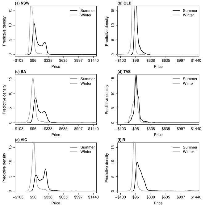
Figure 3: Predictive densities for electricity prices at midday on 15 Jan 2019 (labelled ‘summer’) and 15 July 2019 (labelled ‘winter’). Panels (a) to (e) give the densities for prices in each of the five regions, and panel (f) for the demand-weighted system price. The horizontal axis is on the logarithmic scale.

5.4 Benchmarking

To validate our model we compare its predictive accuracy for $\bar{Y}$ with those from other multivariate regression models using 10-fold cross-validation. The root mean square error (RMSE) is used to measure point prediction accuracy, and the log-score (LS) and cumulative ranked probability score (CRPS) measure distributional predictive accuracy. The competing models are:

• MVC.prior1 and MVC.prior2: our proposed approach using priors 1 and 2 for $\Sigma$.

• MVC.add.prior and MVC.add.prior2: as above, but with an additive basis for demand covariates, with $F$ comprising univariate thin plate spline basis terms.

• MVC.lin.prior1 and MVC.lin.prior2: as above, but with a linear basis over demand covariates, so that $F$ comprises only linear terms.

• MVN.lin: a Gaussian SUR model with linear regression terms.

• MVN.lin.het and MVN.lin.cov: conditionally Gaussian SUR model with linear regression terms and the marginal variances (lin.het) and also entries of a Cholesky factor of the correlation matrix (lin.cov) being linear functions of the demand covariates.

• MVN.add, MVN.add.het and MVN.add.cov: same as the MVN models, but with additive functions of the demand covariates using univariate thin plate splines.

• NOC: A Gaussian copula model with the marginals for each regional price given by multivariate regressions using the same basis as MVC.prior1/MVC.prior2.

The models denoted MVC are the proposed regression copula models, but with differing function bases. The models denoted MVN are the conditionally Gaussian models of Muschinski et al. (2022) estimated using the R-package “mvnchol”. The model denoted NOC employs the covariates to define nonlinear regressions in the marginals, as in Pitt et al. (2006); Song et al. (2009), rather than to specify the copula process.

Table 2: Electricity prices. Australian NEM system-wide electricity price predictive accuracy

	CRPS	LS	RMSE
Multivariate Regression Copula Models
MVC.prior1	0.01560	-2.23568	0.00167
MVC.prior2	0.01563	-2.24026	0.00167
MVC.add.prior1	0.01560	-2.23422	0.00178
MVC.add.prior2	0.01568	-2.23519	0.00178
MVC.lin.prior1	0.01856	-1.98366	0.00228
MVC.lin.prior2	0.01849	-2.00912	0.00226
Conditionally Gaussian Models
MVN.lin	0.01809	-1.45180	0.00182
MVN.lin.het	1.29217	-0.04494	0.50086
MVN.lin.cov	1.95226	0.21337	36.71676
MVN.add	0.16709	0.58704	0.00161
MVN.add.het	0.45309	-0.43186	0.12253
MVN.add.cov	0.39934	-0.14563	0.29181
Gaussian Copula with Regression Marginals
NOC	0.01807	-2.01589	0.00199

Rows give results using different distributional regression methods. Predictive accuracy is computed using 10-fold CV, and measured using RMSE (point), LS and CRPS (distributional). Lower values of all metrics correspond to higher accuracy. The approach proposed in this paper is most accurate.

Table 2 reports the predictive accuracy metrics and we observe that (i) Prior 1 outperforms Prior 2, (ii) our proposed MVC models dominate, (iii) the MVC models that capture the relationship between demand and price as nonlinear and multivariate are most accurate, and (iv) it is better to capture the impact of demand through the regression copula, rather than through regression marginals as in the NOC model.

6 Likelihood-free Inference for Tree Species Abundance

We now consider an application of our methodology to likelihood-free inference (LFI) for tree species abundance survey data. The data are from Chisholm et al. (2014), and are species counts from five complete censuses of trees for a period spanning 1987-2005 in a 50 ha plot in Pasoh, Malaysia. Data from a second site is used for setting an informative prior.

We first describe the stochastic model considered by Chisholm et al. (2014). This is followed by a discussion of LFI and how to use distributional regression to perform such inference. Finally, we present the results of our analysis. We compare these to univariate marginal posterior estimation of Klein et al. (2021), and these authors benchmark their approach against a range of alternative LFI methods. The focus is on how multivariate estimation improves inference in this example, compared to univariate estimation.

6.1 Model for tree species abundance

Consider a forested area (a “site”) that is censused at various intervals to track the abundances of the tree species present. Let $N_{it}$ denote the abundance of tree species $i$ for census $t$, for $t=1,\dots,T=5$ and $i=1,\dots,I=814$. There are $T-1$ census intervals with durations $\Delta T_{it}$, for $t=1,\dots,T-1$, $i=1,\dots,I$. The census intervals are species specific, since the average census time for trees of a given species depends on their spatial distribution. Let $S_{it}$ denote the number of trees of species $i$ surviving within census interval $t$. Define $A_{it}=N_{i(t+1)}-S_{it}$, so that $A_{it}$ represents recruitment in census interval $t$. Chisholm et al. (2014) model the data for each census interval separately, conditionally on the initial abundance for the interval. For census interval $t=1,\ldots,T-1$, the model (conditional on $N_{it}$, $i=1,\dots,I$) is

$$S_{it}|N_{it} \sim\text{Binomial}(N_{it},\exp(-\mu_{it}\Delta T_{it})),$$ (13)

$$A_{it}|S_{it},N_{it} \sim\text{Poisson}\left(N_{it}\left\{\exp(\rho_{it}\Delta T_{it})-\exp(-\mu_{it}\Delta T_{it})\right\}\right),$$ (14)

where the parameters $\mu_{it},\rho_{it}$ are instantaneous mortality and growth rates, respectively. The mortality and growth rates are given hierarchical priors,

$$\mu_{it}|\rho_{it} \sim\text{LN}(\Omega_{t},\sigma_{t}^{2})I(\mu_{it}>-\rho_{it}),\;\;\;\;\rho_{it}\sim\text{ALD}(c_{t},\phi_{1t},\phi_{2t}),$$

where $\text{LN}(\mu,\sigma^{2})I(A)$ denotes a log-normal distribution with parameters $\mu$ and $\sigma^{2}$, truncated to region $A$, and $\text{ALD}(c,\phi_{1},\phi_{2})$ denotes an asymmetric Laplace distribution with density

$$f(x;c,\phi_{1},\phi_{2}) =\left\{\begin{array}[]{cc}k\exp((x-c)\phi_{2})&\mbox{$x<c$}\\ k\exp((c-x)\phi_{1})&\mbox{$x\geq c$},\end{array}\right.$$

and $k=\phi_{1}\phi_{2}/(\phi_{1}+\phi_{2})$. The prior for $\rho_{it}$ is truncated to ensure that the mean of the Poisson distribution in (14) is positive. The priors on the hyperparameters $\Omega_{t}$, $\sigma_{t}^{2}$, $c_{t}$, $\phi_{1t}$ and $\phi_{2t}$ are described later. Chisholm et al. (2014) use MCMC to evaluate the posterior of the parameters for each census interval, where for computational tractability an approximation of the likelihood was used.

6.2 Likelihood-free inference

LFI is used to compute Bayesian inference for models where computing the likelihood is impractical. Suppose we have data $\mathcal{D}$ with observed value denoted $\mathcal{D}_{\text{obs}}$, and a model for the data involving parameters $\psi$, specified by a density $p({\mathcal{D}}|\text{\boldmath$\psi$})$. The prior density for $\psi$ is $p(\text{\boldmath$\psi$})$. For the joint density $p(\text{\boldmath$\psi$},{\mathcal{D}})=p(\text{\boldmath$\psi$})p({\mathcal{D}}|\text{\boldmath$\psi$})$, the conditional density for $\psi$ given ${\mathcal{D}}={\mathcal{D}}_{\text{obs}}$ is the posterior density $p(\text{\boldmath$\psi$}|{\mathcal{D}}_{\text{obs}})$. From this observation, if we simulate samples $\{(\text{\boldmath$\psi$}_{i},{\mathcal{D}}_{i})\}_{i=1}^{n}$ independently from $p(\text{\boldmath$\psi$})p({\mathcal{D}}|\text{\boldmath$\psi$})$, a distributional regression model can be fitted using these simulations as training data to estimate $p(\text{\boldmath$\psi$}|{\mathcal{D}}_{\text{obs}})$. When using the distributional regression model outlined here, set $\bm{Y}_{i}=\text{\boldmath$\psi$}_{i}$, $\text{\boldmath$x$}_{i}={\mathcal{D}}_{i}$, and consider the multivariate predictive density of $\bm{Y}_{n+1}$ given $\text{\boldmath$x$}_{n+1}={\mathcal{D}}_{\text{obs}}$ as the estimate of the multivariate posterior density. This procedure only requires the simulation of the training data from the model, and not evaluation of the likelihood $p({\mathcal{D}}|\text{\boldmath$\psi$})$.

Often LFI methods do not use the raw data ${\mathcal{D}}$ for estimating the posterior density, but instead use a lower-dimensional summary statistic vector $\text{\boldmath$H$}_{\text{obs}}=\text{\boldmath$H$}({\mathcal{D}}_{\text{obs}})$. There can be two advantages to doing this. The first is computational, where the reduction in dimension (without losing too much information about $\psi$) can also reduce Monte Carlo variation of posterior estimates using LFI algorithms. The second is to make inference robust to the misspecification of the stochastic model. Lewis et al. (2021) recently highlight and greatly develop the “restricted likelihood” approach to Bayesian inference with misspecified models, where a posterior distribution is constructed by conditioning on a summary statistic rather than the full data. The use of a summary statistic allows us to discard information that cannot be matched under the assumed model, with the intended use of the model able to guide what summaries the analyst should focus on matching. Even in models with tractable likelihood, the likelihood for summary statistics may be intractable, so that LFI methods are attractive for restricted likelihood computation (Nott et al., 2024).

We implement a restricted likelihood approach for analyzing the tree species abundance model, where there is concern about the adequacy of the binomial and Poisson models for survival and recruitment. We consider LFI based on simulation of data replicates from (13) and (14), after simulating parameters from the prior. We use the following hyperpriors:

$$\Omega_{t} \sim N(-3.3,1.2^{2}), c_{t} \sim N(0.07,0.08^{2}),$$

$$\sigma_{t}^{2} \sim IG(2,1), \phi_{1t},\phi_{2t} \sim IG(3,200),$$

$t=1,\dots T-1$, where $IG(a,b)$ is an inverse gamma distribution with shape $a$ and scale $b$. The hyperpriors were chosen after examining estimates of growth and mortality rates from another site (Barro Colorado Island in Panama), devising priors summarizing the variation of these estimates, and then making these more dispersed to account for inter-site differences and to avoid any resulting prior-data conflicts. The data used for both sites can be found in the supplementary materials of Condit et al. (2006).

We use our multivariate regression model to estimate the joint posterior distribution of the parameters $\Omega_{t},\sigma_{t}^{2},\phi_{1t},\phi_{2t}$, $t=1,\dots,T-1$. These are the parameters of main scientific interest in the model, as they enable a crude estimate of the amount of variation in abundance fluctuations due to environmental variance and to demographic variance respectively at different times. Environmental variance is variability due to temperature, rainfall, pests and other environmental factors. Demographic variance is variability due to the stochastic nature of birth and death processes and variation of birth and death rates within a population due to individual specific factors. There are other relevant sources of variation also, see Chisholm et al. (2014) for further discussion.

Temporal environmental variability is correlated across individuals, and if this is the main factor driving abundance fluctuations it is expected that the variance of abundance fluctuations should scale roughly quadratically with initial abundance. On the other hand, if demographic variability drives abundance levels, simple population dynamics models exhibit variance of abundance changes scaling linearly with abundance levels. In practice, a scaling exponent between $1$ and $2$ is usually observed and for the data considered here scaling exponents near $2$ provide a good fit for common species, while values near $1$ provide a good fit for rare species. This suggests that environmental variability is driving abundance levels for common species while demographic variability is most important for rare species, consistent with theoretical expectations.

In discussing limitations of their model, Chisholm et al. (2014, p. 5) mention that the assumption of binomial and Poisson distributions for survival and recruitment may be too simple. Hence our motivation for using LFI here is to fit directly to scientifically meaningful summary statistics so that the fitted model is fit-for-purpose for understanding sources of variability driving population dynamics. The summary statistic likelihood is intractable, so LFI methods are essential for computation. The summary statistics we define relate to direct estimates of scaling exponents of variability of abundance fluctuations with initial abundance, as well as overall growth and mortality. A detailed description of the summary statistics is given in the supplementary material. We will see that a restricted likelihood analysis allows the model to match the summaries, whereas a conventional Bayesian analysis based on the full data using the approximate full likelihood method in Chisholm et al. (2014) does not.

6.3 Distributional regression for posterior approximation

We consider analyses to approximate the joint posterior density for $\text{\boldmath$\psi$}_{t}=(\Omega_{t},\sigma_{t}^{2},c_{t},\phi_{1t},\phi_{2t})^{\top}$ using summary statistics $\text{\boldmath$H$}_{t}$ for census interval $t=1,\ldots,T-1$. In forming the regression predictor in (4) we use a thin plate regression spline basis expansion as in Section 5 with $k=50$ knots chosen as the centroids of a $k$-means clustering. With a smoothness penalty of order 3 we thus arrive at 70 basis functions.

We are interested in inference on $\text{\boldmath$\psi$}_{t}$ because it gives an approximate but interpretable partitioning of the abundance variation into environmental and demographic components at time $t$, leading to

$$\mbox{Var}(N_{t+1}\mid N_{t}=N)\approx N^{2}\Delta T_{t}^{2}v_{e}+N\Delta T_{t}v_{d}$$ (15)

where $v_{e}=\mbox{Var}(\rho_{t})$ and $v_{d}=E(\rho_{t})+2E(\mu_{t})$, see (S8) in the supporting materials of Chisholm et al. (2014). Following these authors we estimate $\text{\boldmath$\psi$}_{t}$ at each census interval separately and compare the original approximate likelihood-based estimates of Chisholm et al. (2014) (denoted by CTFS, obtained using the CTFS R package) with our multivariate regression copula with priors 1 and 2 (denoted by MVC prior1, MVC prior 2) and the univariate regression copula approach of Klein et al. (2021) (denoted by UVC). The latter three LFI methods use the summary statistics and are trained with $n=5,000$ samples $\{\text{\boldmath$\psi$}_{t}^{(r)},{\mathcal{D}}_{t}^{(r)}\}_{r=1}^{n}$ of parameters and data sets ${\mathcal{D}}_{t}^{(r)}=\{S_{1t}^{(r)},A_{1t}^{(r)},\ldots,S_{It}^{(r)},A_{It}^{(r)}\}$ of the same size as the observed data. We train MVC, UVC with 30,000 VI iterations, $K=1$ and $M=10$. Unlike many other LFI methods, our approach is “amortized”, which means that after model training, inference and prediction on any new data set can be performed directly. For evaluation of the results, we generated 1,000 additional test samples.

6.4 Results

Marginal calibration

One criterion for evaluating the probabilistic forecast at (12) is its “calibration”, which is its statistical consistency with the observations (Gneiting et al., 2007). Klein et al. (2021) discuss marginal calibration properties of probabilistic forecasts from distributional regression methods, and demonstrate that the univariate version of our proposed copula method has good marginal calibration properties. They also discuss the application of regression copula distributional regression for LFI, although they are only able to produce estimates of univariate marginal posterior distributions because their method is univariate. For LFI, marginal calibration corresponds to the average estimated posterior distribution, for datasets drawn from the prior predictive distribution, being equal to the prior. This calibration property holds for the true posterior density, since we can write

$$p(\text{\boldmath$\psi$})=\int p(\text{\boldmath$\psi$})p({\mathcal{D}}|\text{\boldmath$\psi$})\,d{\mathcal{D}}=\int p({\mathcal{D}})p(\text{\boldmath$\psi$}|{\mathcal{D}})\,d{\mathcal{D}},$$

showing that the expectation of the true posterior density is the prior, averaging over data drawn from the prior predictive. For an LFI method, although good calibration doesn’t guarantee accuracy it is certainly desirable, and poor calibration indicates possible posterior inaccuracy. Figure 4 demonstrates that both the UVC method and also our proposed MVC method are marginally calibrated. It plots the average posterior density estimates (solid lines) from the posterior predictive densities in the test samples versus a probability histogram of the prior.

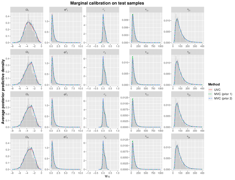
Figure 4: Ecology data. Plots of average estimated posterior densities for UVC and MVC with priors 1 and 2 (solid lines) and prior samples (grey histograms).

Posterior estimation and posterior predictive densities of summaries

Figure B in the supplementary material shows the estimated marginal posteriors together with a histogram of samples from the priors for all census intervals. Generally, the MVC and UVC methods agree well with each other, but the estimates from the CTFS method without summary statistics differ. Figure 5 summarizes the posterior predictive densities of summary statistics obtained by 10,000 samples from the estimated posterior distributions for each method and for census interval 2. The vertical lines indicate the observed summary statistic values. For this census interval, it can be seen that the likelihood-based full data method CTFS produces a posterior predictive density for the first summary statistic for which the observed value is out in the tails, indicating that the fitted model cannot match the observed value. A similar result can be seen for census interval 4 (results not shown). The first summary statistic is a pooled estimate of the scaling exponent of variance abundance fluctuations with initial abundance, which is an important quantity in the scientific study. It is expected on theoretical grounds that the scaling exponent would vary by the initial abundance, but the pooled estimate is used for summarizing the data. The inability to reproduce this quantity is likely to be reflected in misleading estimates of demographic variance from (15). To investigate this, Table 3 summarizes the demographic variance values obtained from (15). The table shows these variances for three species that correspond to the three quartiles of abundances at census interval 1 and follows these three species over time. Then (15) is computed for the CTFS, UVC and MVC methods (with priors 1 and 2), and using either plug-in hyperparameter estimates or samples from the posterior approximation, with the exception of UVC for which there is no joint posterior estimate available. In general the CTFS method gives very different estimates of demographic variance to the other summary statistic based approaches, which can be attributed partly to model misspecification, and warns of sensitivity of this variance to modelling assumptions. Also, we see that accounting for posterior uncertainty using joint posterior samples makes a big difference to the estimated variances for MVC, so that not being able to account for this parameter uncertainty for the UVC method, which is univariate, is a limitation of that approach.

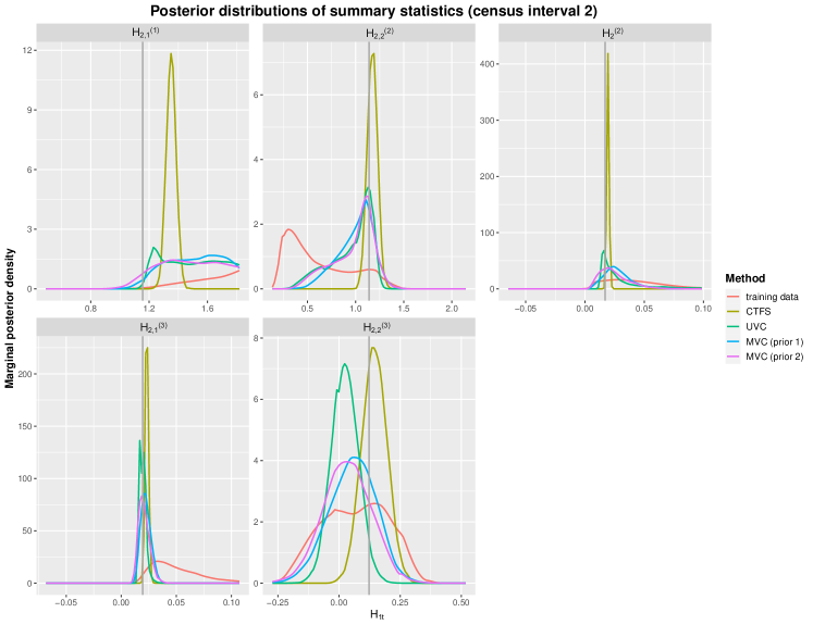
Figure 5: Ecology data. Posterior predictive densities of five summary statistics for census interval 2. The first summary statistic considered (top left graph) is an estimate of the scaling exponent of variance of abundance fluctuations with initial abundance.

	CTFS	CTFS(*)	UVC	MVC	MVC	MVC	MVC
census, species				(prior 1)	(prior 1,*)	(prior 2)	(prior 2,*)
$t=1,i=343$	2.99	3.01	5.27	4.79	9.04	5.28	9.35
$t=2,i=343$	14.67	14.83	9.50	10.47	18.39	9.23	16.76
$t=3,i=343$	11.51	11.04	12.14	13.53	22.30	12.63	20.81
$t=4,i=343$	324.01	337.00	94.55	119.09	199.10	93.91	161.86
$t=1,i=284$	21.51	21.42	41.87	40.87	78.34	42.60	77.88
$t=2,i=284$	162.21	165.09	65.84	91.51	158.74	65.82	118.32
$t=3,i=284$	63.82	61.07	80.37	93.63	146.56	84.96	129.79
$t=4,i=284$	216.96	225.90	67.27	82.85	139.28	67.83	115.25
$t=1,i=540$	130.98	129.41	279.88	285.79	560.29	292.14	542.48
$t=2,i=540$	966.81	983.22	304.97	491.29	846.51	309.97	555.47
$t=3,i=540$	210.95	201.31	293.08	349.71	526.95	301.96	456.39
$t=4,i=540$	483.89	501.47	134.64	169.71	285.72	134.39	228.24

Table 3: Ecology data. Demographic variance for three selected species at each census interval. Values for UVC have been computed based on the posterior mean estimate of $\psi$. For CTFS and MVC we report results based on the respective point estimates, but also using samples from the joint posteriors (indicated with *).

7 Discussion

This paper outlines a new scalable multivariate distributional regression method, which has a number of unique features. It combines marginal distributions $G_{1},\ldots,G_{p}$ with the implicit copula $C_{1:n}$ of a multivariate regression model in which the regression coefficients are integrated out. The flexible marginal specification ensures that the approach exhibits good marginal calibration in uncertainty quantification. This proves important in both an econometric prediction application, as well for LFI. In the copula construction we use a novel multivariate extension of the horseshoe prior with attractive properties and consider two priors for the cross-equation correlation matrix $\Sigma$.

The equations at (4) share a common covariate vector $\text{\boldmath$x$}_{i}$ for each response variable. This may limit the usefulness of the method in some examples, although there are many applications with a common covariate across dimensions, including LFI. The method allows for sizable covariate vectors (e.g. $q=50$ and $q=70$ in our two applications) and large sample sizes (e.g. $n=17,250$ in one of our application). Estimation speed is also important when using distributional regression methods to conduct LFI. We achieve this here by applying efficient variational inference methods to an augmented posterior, so that our estimation approach is scalable. Finally, regularization is provided by our novel multivariate extension of the horseshoe prior. This has standard horseshoe priors for the coefficients from each equation as marginals, yet is a dependent prior in an analogous fashion as a g-prior, and may have applications beyond that discussed here.

Appendix A Priors for $\Sigma$

Prior 1: matrix logarithm

Let $\text{vecl}(A)$ denote the half vectorization of the strictly lower triangular elements of a symmetric matrix $A$, then set $\text{\boldmath$\upsilon$}=\text{vecl}(\log(\Sigma))$, where $\log(\Sigma)$ is the matrix logarithm of $\Sigma$. Archakov and Hansen (2021) show there is a one-to-one mapping between $\Sigma$ and $\upsilon$. To compute $\Sigma$ from $\upsilon$ these authors propose the following recursive algorithm. For a vector $\text{\boldmath$d$}\in\mathbb{R}^{p}$, write $A(\text{\boldmath$\upsilon$},\text{\boldmath$d$})$ for the $p\times p$ symmetric matrix with diagonal elements $d$ and $\text{vecl}(A(\text{\boldmath$\upsilon$},\text{\boldmath$d$}))=\text{\boldmath$\upsilon$}$. There is a unique value $\text{\boldmath$d$}^{*}$ such that $\exp(A(\text{\boldmath$d$}^{*},\text{\boldmath$\upsilon$}))$ is a correlation matrix, where $\exp(A)$ is the matrix exponential of $A$. To find $\text{\boldmath$d$}^{*}$, let $\text{\boldmath$d$}^{(0)}\in\mathbb{R}^{p}$ denote some initial guess for $d$. Consider the recursion

$$\text{\boldmath$d$}^{(k+1)}=\text{\boldmath$d$}^{(k)}-\log\text{diag}(\exp(A(\text{\boldmath$\upsilon$},\text{\boldmath$d$}^{(k)}))),$$

where $\text{diag}(B)$ denotes the vector of diagonal entries of $B$ and the logarithm is taken element-wise. Archakov and Hansen (2021) show that $\lim_{k\rightarrow\infty}\text{\boldmath$d$}^{(k)}=\text{\boldmath$d$}^{*}$ and that the algorithm converges exponentially fast. Moreover, an expression for the Jacobian $\frac{\partial^{p(p-1)/2}}{\partial\text{\boldmath$\upsilon$}}\text{vecl}(\Sigma)$ is given in Section 4.3 of Archakov and Hansen (2021), which is required when computing variational inference with Prior 1.

We use a ridge prior $\text{\boldmath$\upsilon$}\sim N(\bm{0},\sigma_{\upsilon}^{2}I_{p(p-1)/2})$ with an inverse gamma hyper-prior $\sigma_{\upsilon}^{2}\sim\mbox{IG}(a_{\upsilon},b_{\upsilon})$, with $a_{\upsilon}=b_{\upsilon}=0.001$. With this prior, the copula parameters are $\text{\boldmath$\vartheta$}=\{\text{\boldmath$\upsilon$},\log(\sigma^{2}_{\upsilon}),\text{\boldmath$\theta$}\}$.

Prior 2: factor re-parameterization

Set $\Upsilon=GG^{\top}+D$, where $D=\mbox{diag}(d)$ and $G=\{g_{ij}\}_{i=1:p,j=1:K}$ is $p\times K$, with $K\ll p$, then a factor prior uses the parameterization

$$\Sigma=\mbox{diag}(\Upsilon)^{-1/2}\Upsilon\mbox{diag}(\Upsilon)^{-1/2}\\ =\widetilde{G}\widetilde{G}^{\top}+\widetilde{D}$$

where

$$\mbox{diag}(\Upsilon)^{-1/2} = \mbox{diag}\left((d_{1}+\sum_{j=1}^{K}g_{1j}^{2})^{-1/2},\ldots,(d_{p}+\sum_{j=1}^{K}g_{pj}^{2})^{-1/2}\right)\,,$$

$$\widetilde{G} = \mbox{diag}(\Upsilon)^{-1/2}G=\{\tilde{g}_{ij}\}_{i=1:p,j=1:K}$$

$$\tilde{g}_{ij} = g_{ij}/\sqrt{d_{i}+\sum_{j=1}^{K}g_{ij}^{2}}$$

$$\widetilde{D} = \mbox{diag}\left(\frac{d_{1}}{d_{1}+\sum_{j=1}^{K}g_{1j}^{2}},\ldots,\frac{d_{p}}{d_{p}+\sum_{j=1}^{K}g_{pj}^{2}}\right)$$

Setting $D=I$, the upper triangle of $G$ to zeros (i.e. $g_{ij}=0$ for $j>i$) and the leading diagonal elements of $G$ positive, identifies the parameters. Murray et al. (2013) point out that (approximately) uninformative priors for $g_{ij}$ are informative for $\Sigma$, and suggest using a Generalized Double Pareto prior for each element $j\leq i$ with density

$$\pi(g_{ij})=\frac{a_{g}}{2b_{g}}\left(1+\frac{|g_{ij}|}{b_{g}}\right)^{-(a_{g}+1)}\,,$$

and $a_{g}=3$ and $b_{g}=1$, which is written GPD(3,1). With this prior, the real-valued parameters are $\text{\boldmath$g$}^{0}=(\mbox{vecl}(G),l_{11},\ldots,l_{KK})^{\top}$, where the logarithm $l_{ii}=\log(g_{ii})$ for $i=1,\dots,K$, and the copula parameters are $\text{\boldmath$\vartheta$}=\{\text{\boldmath$g$}^{0},\text{\boldmath$\theta$}\}$.

References

- (1)
- Acar et al. (2013) Acar, E. F., Craiu, V. R. and Yao, F. (2013). Statistical testing of covariate effects in conditional copula models, Electronic Journal of Statistics 7: 2822–2850.
- Archakov and Hansen (2021) Archakov, I. and Hansen, P. R. (2021). A new parametrization of correlation matrices, Econometrica 89(4): 1699–1715.
- Brown et al. (1998) Brown, P. J., Vannucci, M. and Fearn, T. (1998). Multivariate Bayesian variable selection and prediction, Journal of the Royal Statistical Society: Series B 60(3): 627–641.
- Carvalho et al. (2009) Carvalho, C. M., Polson, N. G. and Scott, J. G. (2009). Handling sparsity via the horseshoe, in D. van Dyk and M. Welling (eds), Proceedings of the Twelth International Conference on Artificial Intelligence and Statistics, Vol. 5 of Proceedings of Machine Learning Research, pp. 73–80.
- Carvalho and Polson (2010) Carvalho, C. M. and Polson, Nicholas, G. (2010). The horseshoe estimator for sparse signals, Biometrika 97(2): 465–480.
- Chisholm et al. (2014) Chisholm, R. A., Condit, R., Rahman, K. A. et al. (2014). Temporal variability of forest communities: empirical estimates of population change in 4000 tree species, Ecology Letters 17(7): 855–865.
- Condit et al. (2006) Condit, R., Ashton, P., Bunyavejchewin, S. et al. (2006). The importance of demographic niches to tree diversity, Science 313(5783): 98–101.
- Ghosh et al. (2021) Ghosh, R. P., Mallick, B. and Pourahmadi, M. (2021). Bayesian Estimation of Correlation Matrices of Longitudinal Data, Bayesian Analysis 16(3): 1039 – 1058.
- Gneiting et al. (2007) Gneiting, T., Balabdaoui, F. and Raftery, A. E. (2007). Probabilistic forecasts, calibration and sharpness, Journal of the Royal Statistical Society: Series B 69(2): 243–268.
- Hothorn et al. (2014) Hothorn, T., Kneib, T. and Bühlmann, P. (2014). Conditional transformation models, Journal of the Royal Statistical Society: Series B (Statistical Methodology) 76: 3–27.
- Jordan and Jacobs (1994) Jordan, M. I. and Jacobs, R. A. (1994). Hierarchical mixtures of experts and the EM algorithm, Neural Computation 6(2): 181–214.
- Kingma and Welling (2014) Kingma, D. P. and Welling, M. (2014). Auto-encoding variational Bayes, Proceedings of the 2nd International Conference on Learning Representations (ICLR) 2014.
- Klein et al. (2021) Klein, N., Nott, D. J. and Smith, M. S. (2021). Marginally calibrated deep distributional regression, Journal of Computational and Graphical Statistics 30(2): 467–483.
- Klein and Smith (2019) Klein, N. and Smith, M. S. (2019). Implicit copulas from Bayesian regularized regression smoothers, Bayesian Analysis 14(4): 1143–1171.
- Koenker and Bassett (1978) Koenker, R. and Bassett, G. (1978). Regression quantiles, Econometrica 46(1): 33–50.
- Lewis et al. (2021) Lewis, J. R., MacEachern, S. N. and Lee, Y. (2021). Bayesian restricted likelihood methods: Conditioning on insufficient statistics in Bayesian regression (with discussion), Bayesian Analysis 16(4): 1393 – 2854.
- Li et al. (2021) Li, Y., Datta, J., Craig, B. A. and Bhadra, A. (2021). Joint mean–covariance estimation via the horseshoe, Journal of Multivariate Analysis 183: 104716.
- Murray et al. (2013) Murray, J. S., Dunson, D. B., Carin, L. and Lucas, J. E. (2013). Bayesian Gaussian copula factor models for mixed data, Journal of the American Statistical Association 108(502): 656–665.
- Muschinski et al. (2022) Muschinski, T., Mayr, G. J., Simon, T., Umlauf, N. and Zeileis, A. (2022). Cholesky-based multivariate Gaussian regression, Econometrics and Statistics 29: 261–281.
- Nott et al. (2024) Nott, D. J., Drovandi, C. and Frazier, D. T. (2024). Bayesian inference for misspecified generative models, To appear in Annual Review of Statistics and Its Application 11.
- Ong et al. (2018) Ong, V. M., Nott, D. and Smith, M. (2018). Gaussian variational approximation with a factor covariance structure, Journal of Computational and Graphical Statistics 23(3): 465–478.
- Pitt et al. (2006) Pitt, M., Chan, D. and Kohn, R. (2006). Efficient Bayesian inference for Gaussian copula regression models, Biometrika 93(3): 537–554.
- Rezende et al. (2014) Rezende, D. J., Mohamed, S. and Wierstra, D. (2014). Stochastic backpropagation and approximate inference in deep generative models, in E. P. Xing and T. J. T. (eds), Proceedings of the 29th International Conference on Machine Learning, ICML 2014.
- Rigby and Stasinopoulos (2005) Rigby, R. A. and Stasinopoulos, D. M. (2005). Generalized additive models for location, scale and shape, Journal of the Royal Statistical Society: Series C (Applied Statistics) 54(3): 507–554.
- Smith and Klein (2021) Smith, M. S. and Klein, N. (2021). Bayesian inference for regression copulas, Journal of Business & Economic Statistics 39(1): 712–728.
- Smith and Kohn (2000) Smith, M. S. and Kohn, R. (2000). Nonparametric seemingly unrelated regression, Journal of Econometrics 98(2): 257–281.
- Smith and Shively (2018) Smith, M. S. and Shively, T. S. (2018). Econometric modeling of regional electricity spot prices in the australian market, Energy Economics 74: 886–903.
- Song (2000) Song, P. (2000). Multivariate dispersion models generated from Gaussian copula, Scandinavian Journal of Statistics 27(2): 305–320.
- Song et al. (2009) Song, P. X.-K., Li, M. and Yuan, Y. (2009). Joint regression analysis of correlated data using Gaussian copulas, Biometrics 65(1): 60–68.
- Weron (2014) Weron, R. (2014). Electricity price forecasting: A review of the state-of-the-art with a look into the future, International journal of forecasting 30(4): 1030–1081.
- Wilson and Ghahramani (2010) Wilson, A. G. and Ghahramani, Z. (2010). Copula processes, in J. Lafferty, C. Williams, J. Shawe-Taylor, R. Zemel and A. Culotta (eds), Advances in Neural Information Processing Systems, Vol. 23.
- Wood (2003) Wood, S. N. (2003). Thin Plate Regression Splines, Journal of the Royal Statistical Society Series B: Statistical Methodology 65(1): 95–114.
- Yan and Trück (2020) Yan, G. and Trück, S. (2020). A dynamic network analysis of spot electricity prices in the australian national electricity market, Energy Economics 92: 104972.
- Zellner (1962) Zellner, A. (1962). An efficient method of estimating seemingly unrelated regressions and tests for aggregation bias, Journal of the American Statistical Association 57(298): 348–368.