The Madrid-2019 force field for electrolytes in water using TIP4P/2005 and scaled charges: extension to the ions F^-, Br^-, I^-, Rb⁺, Cs⁺.

Abstract

In this work, an extension of the Madrid-2019 force field is presented. We have added the cations Rb⁺ and Cs⁺ and the anions F^-, Br^- and I^-. These ions were the remaining alkaline and halogen ions not previously considered in the Madrid-2019 force field. The force field, denoted as Madrid-2019-Extended, does not include polarizability, and uses the TIP4P/2005 model of water and scaled charges for the ions. A charge of $\pm$0.85 $e$ is assigned to monovalent ions. The force field developed provides an accurate description of the aqueous solution densities over a wide range of concentrations up to the solubility limit of each salt studied. Good predictions of viscosity and diffusion coefficients are obtained for concentrations below 2 m. Structural properties obtained with this force field are also in reasonable agreement with the experiment. The number of contact ion pairs has been controlled to be low so as to avoid precipitation of the system at concentrations close to the experimental solubility limit. A comprehensive comparison of the performance for aqueous solutions of alkaline halides of force fields of electrolytes using scaled and integer charges is now possible. This comparison will help in the future to learn about the benefits and limitations of the use of scaled charges to describe electrolyte solutions.

a) Corresponding author: cvega@quim.ucm.es

I Introduction

Life started from the seas and for this reason, water is the main component of the cells. However, water is not alone in the oceans, since they contain a certain amount of several salts (NaCl being the most abundant component). Not surprisingly ions are also present in living organisms. Arrhenius was the first to suggest that when salts dissolve in water, individual ions are solvated by water, and they are able to conduct the electric current, so that they become denoted as electrolytes.

The solution of electrolytes in water has been studied intensively over the past century, both from an experimental point of view, and from a theoretical point of view. As students we learn the thermodynamics of electrolytes and the Debye-Hückel theory describing their activitiesDebye and Hückel (1923). The birth of computer simulations in the 1950’s brought a new route to study these type of systems. In the 70’s the first simulations of ionic systems were carried outSangster and Dixon (1976); Adams et al. (1977); Heinzinger and Vogel (1974); Vogel and Heinzinger (1975); Heinzinger and Vogel (1976). Aqueous solutions of electrolytes require both a force field for the molecule of water and another one for the ions in water. In the 80’s several force fields for water were proposed (TIP3PJorgensen et al. (1983), TIP4PJorgensen et al. (1983), SPC/EBerendsen et al. (1987)) that are still use widely nowadays. In those force fields the molecule of water is described by a rigid non-polarizable model, typically using a LJ center is located on the oxygen and charges are located in the protons and in other places in the molecule. In early 2000 new models of water were proposed, including TIP4P-EwHorn et al. (2004), TIP5PMahoney and Jorgensen (2001) and TIP4P/2005Abascal and Vega (2005). A common feature of these three models is that they were able to reproduce the maximum in density of pure water. It has been shown that among the rigid non-polarizable models of water TIP4P/2005 is a quite decent oneVega and Abascal (2011); Vega et al. (2009). When describing the force field for the ions, they are often described by a LJ center and a certain charge. The obvious option is to assign a charge of $\pm$Z e to the ions.

Computer simulations of electrolytes are not a fully mature area. In fact it is surprising that most of the simulation studies dealing with these substances do not consider the possibility of evaluating properties such as freezing depression, activity coefficients, salt solubilities, etc. However there has been significant progress over the last ten years and we anticipate that these properties will be computed and will bring some surprises.

There are a large number of models for different alkaline and alkaline-earth salts Smith et al. (2018); Chandrasekhar et al. (1984); Straatsma and Berendsen (1988); Aqvist (1990); Dang (1992); Beglov and Roux (1994); Smith and Dang (1994); Roux (1996); Peng et al. (1997); Weerasinghe and Smith (2003); Jensen and Jorgensen (2006); Lamoureux and Roux (2006); Alejandre and Hansen (2007); Lenart et al. (2007); Joung and Cheatham (2008); Corradini et al. (2010); Callahan et al. (2010); Yu et al. (2010); Reif and Hünenberger (2011); Gee et al. (2011); Deublein et al. (2012); Mao and Pappu (2012); Mamatkulov et al. (2013); Moučka et al. (2013a); Kiss and Baranyai (2014); Kolafa (2016); Elfgen et al. (2016); Pethes (2017); Yagasaki et al. (2020) but standard force fields do not have problems in general (when properly designed) in reproducing the experimental densities for a particular salt, as for instance NaCl. Some force fields such as that proposed by Smith and DangSmith and Dang (1994) were designed for just one electrolyte (NaCl in this case). It is more difficult to find a force field able to describe simultaneously the properties of a large set of salts (i.e NaCl, KCl, MgCl₂ …). Among the fields of this type, the most popular is that proposed by Joung and CheathamJoung and Cheatham (2008) for three particular water models (TIP3PJorgensen et al. (1983), TIP4P-EwHorn et al. (2004), and SPC/EBerendsen et al. (1987)). Since TIP4P/2005Abascal and Vega (2005) is now regarded as a good potential model for waterVega and Abascal (2011) it seems reasonable to develop a force field of electrolytes based on this potential model of water. Dopke et al.Dopke et al. (2020) have recently shown that the force field proposed by Joung and Cheatham could also be used for TIP4P/2005 (by using Lorentz-Berthelot combining rules) provided that one uses either the parameters designed for SPC/E or TIP4P-Ew. We reached a similar conclusion in 2016 when considering NaClBenavides et al. (2016). In any case, although results were reasonable it seems logical to design a force field of electrolytes specifically for the TIP4P/2005 model of water. We started down this route in 2017 for NaClBenavides et al. (2017a), and continued in 2019 presenting a force fieldZeron et al. (2019) of some ions (Li⁺, Na⁺, K⁺, Cl^-,Mg²⁺, Ca²⁺, SO${}_{4}^{2-}$) using TIP4P/2005 water. The choice of the ions in our 2019 paper was not random, but we selected the most abundant ions presented in seawater (which are also the most common ions found in the cells). We have shown that in fact an extremely accurate description of the properties of seawater is possible by using this force fieldZeron et al. (2021). The name of the force field designed for electrolytes in TIP4P/2005 was denoted as Madrid-2019. The purpose of this work is to extend the force field to the ions considered by Joung and Cheatham but not considered when proposing the Madrid-2019 force field, namely the anions F^-, Br^- and I^- and the cations Rb⁺ and Cs⁺. The motivation for this is twofold. On the one hand to extend the applicability of the Madrid-2019 force field, and on the other to allow for a direct comparison between the force field proposed by Joung and Cheatham and the Madrid-2019 force field. The difference between the Joung-Cheatham and the Madrid-2019 force field is not only the choice of the water model but there is also a conceptual idea that makes this comparison specially useful as we will explain later.

Besides the density there are some other properties that are of interest when modelling electrolytes. For instance transport properties such as viscosities or individual diffusion coefficients of the ions and of water. Also the solubility could be of interest (as the solubility of a certain force field should not necessarily correspond to the experimental value). The overwhelming majority of the force fields proposed for electrolytes up to 2011 used integer values (in electron units) of the charge of the ions in solution. How is their performance when describing the properties of these solutions? Let us briefly summarize the situation:

• Regarding transport properties it was shown by Kim et al.Kim et al. (2012) that all force fields underestimated significantly the diffusion coefficient of water at high concentrations. In other words, the force fields overestimated the impact of the salt in reduction of the diffusion coefficient of water.

• Yue and PanagiotopoulosYue and Panagiotopoulos (2019) and also ourselvesZeron et al. (2019) have shown that the viscosity of the solution is dramatically overestimated at high concentrations, sometimes having a viscosity up to 2-4 times larger than in experiments. Bearing in mind the Stokes-Einstein relationDill et al. (2003), this could be expected given the impact of the salt on the diffusion coefficient of water.

• The solubility of most of the force fields using integer charges is quite low when compared to experimentPanagiotopoulos (2020). In the particular case of NaCl the majority of models give a solubility too low by a factor of 2-10Mester and Panagiotopoulos (2015a, b); Jiang and Panagiotopoulos (2016); Espinosa et al. (2016); Jiang et al. (2015). However it is clear after the work of Tanaka and coworkersYagasaki et al. (2020) that when properly designed the use of integer charges still allows for a good description of the solubility. Calculating solubilities via computer simulations is difficult, and only feasible in the last 10 years. For this reason all force fields proposed before 2011 did not consider solubility as a property of interest. Therefore although the use of integer charges should not necessarily provoke a low solubility, it turns out that this was the case for practically all force fields previously designed using integer charges.

• Related to the previous point is the finding that for a number of force fields of electrolytes the number of contact ion pairs (CIP) (i.e a cation in contact with an anion in solutionvan der Vegt et al. (2016); Fennell et al. (2009); Yao and Kanai (2018); Chialvo and Simonson (2006)) was quite high and aggregation of ions (which can be regarded as the initial step of precipitation) was observed in many simulations even at concentrations well below the experimental solubilityGiri and Spohr (2017) (reflecting that the solubility of the force field was well below the experimental one). Actually, ion clustering has been reported for different salts below its experimental solubility limit. This fact can be seen in monovalent salts as NaClMoučka et al. (2013b); Moučka et al. (2012); Alejandre et al. (2009); Alejandre and Hansen (2007), KClAuffinger et al. (2007), divalent salts CaCl₂Martinek et al. (2018), or even sulphates as Na₂SO₄Wernersson and Jungwirth (2010) and Li₂SO₄Pluhařová et al. (2013).

How to go to the next generation of force fields for electrolytes? Ab-initio calculations can be useful as shown by Ding et al.Ding et al. (2014), but these types of calculations are quite expensive from a computational point of view. Introducing polarizability is another possibility (see the work of Kiss and BaranyaiKiss and Baranyai (2013, 2014)) and certainly further research will continue to appear in this area. Notice that including polarization does not guarantee good solubilities, as was shown for the Baranyai force fieldJiang et al. (2015). However it is possible to modify the parameters to improve their predictionsKolafa (2016). First principles calculations and polarizable models will continue being developed in the future. However there is a simple and cheap approach that could improve the performance without extra computational cost. The recipe is simple, and it amounts to using scaled charges for the ions (i.e force fields in which the charge of the ions is $\lambda$$e$ where $\lambda$ is a number smaller than one). The use of scaled charges is common in simulations of ionic liquidsThum et al. (2020); Tenney et al. (2014); Fileti and Chaban (2014); Chaban et al. (2011); Schröder (2012) so exploring this route for electrolytes seems of interest.

Let us briefly describe the “history” of scaled charge models. This was first suggested by Leontyev and StuchebrukhovLeontyev and Stuchebrukhov (2009); Leontyev and Stuchebrukhov (2010a, b); Leontyev and Stuchebrukhov (2011, 2012, 2014) , by realizing that the dielectric constant at high frequencies of non-polarizable models is 1, whereas for water its value is 1.78. With that in mind Leontyev and Stuchebrukhov suggested using a scaled charge of $q_{scaled}($e$)=1/\sqrt{\epsilon_{\infty}}$ for the ions. This lead to a charge of 0.75 Z $e$ for the ions in water. This suggestion was further expanded by Jungwirth and coworkersPluhařová et al. (2013); Kohagen et al. (2014, 2015); Duboué-Dijon et al. (2017); Martinek et al. (2018), and they have developed a potential model for several ions using this value for the charge of the ions. Kann and Skinner follow a somewhat different approachKann and Skinner (2014). If you want to recover the Debye-Hückel law, you should have a force field, describing accurately the density of water, and where the strength of the Coulombic energy between ions at infinite dilution and infinitely large distances should be identical in your model and in experiment. Many force fields of water do not reproduce the experimental value of the dielectric constant of pure water, and that scaled charges should be used to recover the Debye-Hückel law. In the particular case of TIP4P/2005 this results in a value of 0.85 Z $e$ Kann and Skinner (2014). One of us has also pointed out that different charges may be needed to describe the potential energy surface and the dipole moment surfaceVega (2015). Notice that for water models without charges, such as the mWMolinero and Moore (2009), it is possible to design a force field for electrolytes without charges, as is the route followed by Molinero and coworkers and still obtain good resultsDeMille and Molinero (2009). Barbosa and coworkersFuentes-Azcatl and Barbosa (2016) have also used scaled charges. Other authors such as WangLi and Wang (2015) or van der WegtBruce and van der Vegt (2018) have also explored the use of scaled charges. The effect of charge transfer has been also studied by RickSoniat and Rick (2012); Lee and Rick (2011); Soniat and Rick (2014); Soniat et al. (2016) suggesting that part of the charge of the ions is transferred to the adjoining water molecules, as also shown later by Yao et al.Yao et al. (2015). This charge transfer implies that the charge of the ions is not unity and has also been confirmed by quantum calculationsYao and Kanai (2018). The community using scaled charges is growing and Jungwirth and coworkers have summarized the situation in a couple of review papersDuboue-Dijon et al. (2020); Kirby and Jungwirth (2019).

In our previous studies in 2017Benavides et al. (2017a) and in 2019Zeron et al. (2019) we have shown that the use of scaled charges, improves the description of the solubility (at least for NaCl), and the same is true for the viscosity and the diffusion coefficient of water. Yue and Panagiotopoulos have presented further evidence of thatYue and Panagiotopoulos (2019). In fact, we have shown recently that more complex phenomena such as the salting out effect of methane can be quantitatively described with the use of scaled chargesBlazquez et al. (2020). Thus scaled charges seem to improve the description of aqueous solutions of electrolytes. Scaled charges can not describe everything. In fact they can not describe neither the melt, the solid, the vapor-liquid equilibrium of the molten salts, or the kinetics of precipitationKussainova et al. (2020); Panagiotopoulos (2020). Scaled charges are useful only when describing the properties of aqueous solutions of electrolytes but not in problems where the system does not contain water (or has a very small amount).

To sum up in this paper we extend the Madrid-2019Zeron et al. (2019) force field to other monovalent cations and anions belonging to the alkaline group and to the halogens. By doing that we now have a set of parameters for the same set of ions selected by Joung and CheathamJoung and Cheatham (2008), and ready for their use with the TIP4P/2005Abascal and Vega (2005) model of water that was not considered in the original parameterization of Joung and Cheatham. A consequence, is that now a face to face comparison of a good force field designed using integer charges, and a force field designed using scaled charges is possible. We hope that this comparison will shed light on the possible advantages and disadvantages of the use of scaled charges for modelling electrolyte solutions.

II Extending the Madrid-2019 force field to other electrolytes

In this work, an extension (to other ions) of the recently developed Madrid-2019Zeron et al. (2019) force field of scaled charges has been carried out. Madrid-2019Zeron et al. (2019) force field was initially proposed to describe the most common salts present in seawater. In this work we extend the model to the rest of the halogens that remained to be studied (F^-, Br^- and I^-) and to the rest of the cations of the alkaline group (Rb⁺ and Cs⁺). When designing force fields, certain properties are used as the target, and the values of the parameters of the potential are obtained so that these properties are reproduced.

Now we describe in detail the philosophy of the Madrid-2019 force field, and the approach we used to obtain the parameters of the potential. Obtaining parameters of a force field is a difficult job. It requires patience, a good design, and some trial and error. In the future machine learning techniques could certainly help in obtaining the best set of parameters for a certain potential model. It should be recognized from the very beginning that the only way to reproduce experimental results for all properties would be to solve the Schrödinger equation exactly, and to include nuclear quantum effects. If this is not done, your approach will not be able to reproduce “everything” and certain properties will be reproduced but other properties not. These are the main characteristics of the Madrid-2019 force field and the description of how the parameters were obtained:

• Water is described by the TIP4P/2005 model. Ions are described by a Lenard-Jones(LJ) center and a certain charge. In the case of the Madrid-2019 force field, the charge (in electron units) is scaled and its value is 0.85 for monovalents ions and 1.70 for divalent ions. The force field requires one to know the LJ parameters ($\sigma$ and $\epsilon$) of the interaction of a certain ion with the rest of species of the system.

• The Lennard-Jones interaction between an ion and water is described by the ion-oxygen interaction (i.e there is no ion-hydrogen interaction). The reason for that is that in the TIP4P/2005 model of water there is no LJ center on the hydrogen atoms of the molecule of water.

• Lorentz-Berthelot (LB) rules are in general not used. Thus, the parameters of the LJ ion-oxygen interaction and between a cation and an anion are not obtained via the LB combination rule. However, the interaction between two different types of cations and/or two different type of anions (required to study systems having simultaneously several salts as in the case of seawater) are usually given by LB combining rules.

• The force field is transferable. The parameters of the interaction of an ion with other species (water, other ions …) are always the same regardless of the chemical composition of the system.

• In this work, the parameters for the interaction between the ions Cl^-, Li⁺, Na⁺, K⁺, Mg²⁺, Ca²⁺ with water and the crossed interactions between these ions is taken from our previous work in which the force field Madrid-2019Zeron et al. (2019) was introduced. This is an advantage as it reduces the number of parameters to be determined.

• The density of solutions is always considered as a target property. The density of ionic solutions is known with high accuracy from experiments, and we always use it as the target property (at room temperature and pressure).

• The LJ parameters of the ion-water interaction were determined by using the experimental densities for low concentrations (typically up to 1-2 molal , i.e less than 1-2 mols of salt per kilogram of water). The reason for that is that at low concentrations the properties of the solution are given mainly by the ion-water interaction and the impact of ion-ion interaction at low concentrations is quite small. As an example to determine the properties of bromide salts, we shall consider the experimental densities of LiBr, NaBr, KBr, MgBr₂, CaBr₂ and will determine the parameters of the Br^--water interaction using the experimental densities (up to 1-2 $m$) as target. Notice that for these salts the cation-water interaction is already available for the Madrid-2019 force field, so we only need to determine the LJ parameters of the Br^--water interaction.

• Obtaining the Br^--Br^- and Br^--cation interactions (we shall use Br as an example to illustrate how the force field was obtained) is a somewhat more involved process. Again we shall consider the experimental properties of LiBr, NaBr, KBr, MgBr₂, CaBr₂ and used the Madrid-2019 for the cation-cation interaction. Thus one needs to determine the Br^--cation interactions and the Br^--Br^- interaction. This was done using three target properties. The density of the melt should be reproduced (i.e we used as the target a density 20-25 per cent lower than the experimental one). The experimental density of the ionic solutions at high concentrations (close to the experimental solubility limit) should be reproduced. The third constraint is the number of contact ion pairs (CIP). In the study of aqueous electrolyte solutions it is important to evaluate the number of CIP. High values of CIP indicate (indirectly) cluster formation and/or precipitation of the salt. Benavides et al.Benavides et al. (2017b) suggested in a previous work that for 1:1 electrolytes with solubility lower than 11 m the number of CIP must be below 0.5 to be sure that precipitation and/or aggregation of ions has not occurred. This rule will be important in the majority of the salts of this work. (we will discuss later the number of CIP for exceptional cases such as salts with extremely high solubilities). Thus, obtaining Br^--Br^- and Br^--cation interaction is the more difficult step. The reader may wonder why we did not try to reproduce the experimental densities of the melt with scaled charges. We explored this approach but found that often the salt in solution had a large number of CIP and in some cases precipitated. For instance for NaBr we were able to find a set of parameters describing the melt quite well (using scaled charges), but with these parameters the number of CIP in the aqueous solution was large (3.4 at 8 m) and the salt precipitated spontaneously. Thus it seems that to obtain a correct balance between ion-water and ion-ion interactions when using scaled charges, the target density of the melt should be somewhat smaller (20-25 $\%$) than the experimental value.

The last step described above, i.e obtaining for instance Br^--Br^- and Br^--cation interactions requires some further clarifications. The density of the melt is used as a target property. We prefer the melt with respect to the ionic solid as when using empirical force fields the mechanical stability of the experimental solid structure is not guaranteed. Besides this, in the melt one is sampling anion-anion, cation-cation and anion-cation interactions. However the target density was not the experimental density of the melt, but a density typically around 20-25 per cent lower than the experimental one. The reason for that is that we recognize from the very beginning that scaled charges are not adequate to reproduce the properties of pure ionic systems as has been pointed out by Panagiotopoulos and coworkersKussainova et al. (2020); Panagiotopoulos (2020). We observed that when using scaled charges for the melt one obtains a density 20-25 per cent lower than the experimental value and a reasonably low number of CIP avoiding precipitation of the system. However, when replacing the charge with integer values (while keeping the LJ parameters) the experimental density of the melt is reproduced. Our approach will allow one in the future to design and develop a force field in which the charge of the ions is sensitive to the local environment, within the spirit of polarizable models.

Also it is interesting to point out that ideally the solubility of the salt should be considered as a target property. If the solubility is low, then the ions will tend to cluster in solution (or even precipitate spontaneously) and the results of the force field would be unreliable. The calculations of the solubility of a salt is painful from a computational point of view and evaluating it for several trial values of the potential parameters would be beyond current computational limits. However there is a rather simple approach, at least to avoid low values of the solubility.

We have shown in the past for salts with solubilities smaller than 11 m, the number of CIP at the solubility limit of the model is less than 0.5Benavides et al. (2017b). Thus having a number of CIP larger than 0.5 is a warning which indicates that we are not that far from the solubility of the model and the risk of spontaneous precipitation exists (although since nucleation is an activated process, precipitation may occur at concentrations several times higher than the solubility limit, as it happen for the JC-SPC/E model of NaClPatel and Kindt (2019); Jiang et al. (2019)). Therefore we will always force the force field to have a number of CIP less than 0.5 at the experimental value of the solubility (whenever below 11 m). For salts with higher solubilities we will discuss later the number of CIP.

In summary the main goal of the Madrid-2019 force field is to reproduce thermodynamic and transport properties of ionic solutions sacrificing somehow the properties of the melt and/or the solid. The main property of the solution that can not be reproduced by the introduction of scaled charges is the free energy of hydration, which will be low compared to experiments (although it can be corrected in a theoretical wayBlazquez et al. (2020)). Nikitin and FrateNikitin and Del Frate (2019) pointed out that the calculation of the total free energy of hydration, $\Delta$G is better (when including a theoretical correction) by using scaled charges. They consider that the total hydration energy can be divided in two terms. One is the calculated in simulations $\Delta$G_MD and the other one is a theoretical correction denoted as the electronic polarization ($\Delta$G_el). That resembles the situation for water of models like SPC/EBerendsen et al. (1987), TIP4P-EwHorn et al. (2004) or TIP4P/2005Abascal and Vega (2005) that sacrifice the enthalpy of vaporization of water as a target property (in contrast with TIP3PJorgensen et al. (1983), TIP4PJorgensen et al. (1983) and TIP5PMahoney and Jorgensen (2001)) to obtain an overall better description of its properties. Notice though that activity coefficients, osmotic pressures and a number of properties of solution can be still be reproduced even though the absolute value of the hydration free energy is not reproduced. This is so because what really matters is the variation of the Gibbs free energy of the system with the addition of salt, rather than the absolute values of the Gibbs free energies. Transfer of a salt from vacuum to water, will not be described properly by using scaled charges but this is not a big problem as ions are usually not found either in vacuum (due to their low solubilities) in problems of practical interest. Notice, that Vazdar et al.Vazdar et al. (2012) showed in 2012 that using scaled charges (i.e. an electronic continuum correction) allow to describe reasonably well the hydrophobic oil/water interface. In general, they proposed that interfaces with no electronic discontinuity can be reasonably described by using scaled charges.

We shall now present the parameters of the Madrid-2019 extended to the new ions (F^-, Br^-, I^-, Rb⁺, Cs⁺). We shall denote this as Madrid-2019-Extended. The interaction between atoms can be described by two different contributions: The first one, an electrostatic (coulombic) contribution and the second one a van der Waals interaction represented by the LJ potential:

$$u(r_{ij})=\frac{1}{4\pi\varepsilon_{0}}\frac{q_{i}q_{j}}{r_{ij}}+4\epsilon_{ij}\left[\left(\frac{\sigma_{ij}}{r_{ij}}\right)^{12}-\left(\frac{\sigma_{ij}}{r_{ij}}\right)^{6}\right],$$ (1)

where, $q_{i}$ is the ionic charge, $\varepsilon_{0}$ is the vacuum permittivity, $\epsilon_{ij}$ the well depth energy of the LJ potential, and $\sigma_{ij}$ the LJ diameter.

Let us now describe the TIP4P/2005 model of water developed by Abascal and VegaAbascal and Vega (2005). In this model, based on the TIP4P water proposed by Jorgensen et al. Jorgensen et al. (1983), water molecules have four atoms, two hydrogens with charge q${}_{{}_{H}}$, one oxygen which is a LJ site but has no charge and one point M, near the oxygen atom on the symmetric axis, without mass but with charge q${}_{{}_{M}}$. The geometry of water molecules for the TIP4P/2005 model can be described by the following parameters: oxygen-hydrogen distance, d_OH=0.9572 Å, oxygen-M distance, d_OM=0.1546 Å and angle H-O-H=104.52^∘. TIP4P/2005 parameters are collected in Table 1.

Table 1: Force field parameters for water TIP4P/2005 parameters from RefAbascal and Vega (2005).

Molecule		Charge		$\sigma_{ii}$		$\epsilon_{ii}$
		(e)		(Å)		(kJ/mol)
TIP4P/2005
O		0		3.1589		0.7749
H		0.5564
M		-1.1128

We proceed now to present the Madrid-2019-Extended model parameters, which are collected in Tables 2 and 3. We show only the parameters obtained in this work, (when for a certain interaction one reads LB, it means that the interaction has been obtained from the application of the LB combining rule). The salts developed in Madrid-2019 original modelZeron et al. (2019) are denoted as Madrid-2019.

Table 2: Lennard-Jones parameters $\sigma_{ij}$ (in Å) for the ions Li⁺, Na⁺, K⁺, Rb⁺, Cs⁺, Mg²⁺, Ca²⁺, F^-, Cl^-, Br^-, I^- and SO${}_{4}^{2-}$. O_w and O_s are the water an sulfate oxygens.

	F-	Cl-	Br-	I-	Li+	Na+	K+	Rb+	Cs+	Mg2+	Ca2+	Ow	S	Os
F-	3.78982	LB	LB	LB	2.84540	LB	3.46250	3.57250	3.94550	LB	LB	3.77450	LB	LB
Cl-		Madrid-2019	LB	LB	Madrid-2019	Madrid-2019	Madrid-2019	3.99642	4.31854	Madrid-2019	Madrid-2019	Madrid-2019	Madrid-2019	Madrid-2019
Br-			4.82525	LB	2.61450	3.38500	3.79879	3.91725	4.33408	2.65519	3.67052	4.19850	LB	LB
I-				5.04975	3.20470	3.64658	4.00550	4.10288	4.43790	2.82707	3.94181	4.34950	LB	LB
Li+					Madrid-2019	Madrid-2019	Madrid-2019	LB	LB	Madrid-2019	Madrid-2019	Madrid-2019	Madrid-2019	Madrid-2019
Na+						Madrid-2019	Madrid-2019	LB	LB	Madrid-2019	Madrid-2019	Madrid-2019	Madrid-2019	Madrid-2019
K+							Madrid-2019	LB	LB	Madrid-2019	Madrid-2019	Madrid-2019	Madrid-2019	Madrid-2019
Rb+								2.99498	LB	LB	LB	3.54350	LB	3.40000
Cs+									3.521013	LB	LB	3.66290	LB	LB
Mg2+										Madrid-2019	Madrid-2019	Madrid-2019	Madrid-2019	Madrid-2019
Ca2+											Madrid-2019	Madrid-2019	Madrid-2019	Madrid-2019
Ow												Madrid-2019	Madrid-2019	Madrid-2019
S													Madrid-2019	Madrid-2019
Os														Madrid-2019

Table 3: Lennard-Jones parameters $\epsilon_{ij}$ (in kJ/mol) for the ions Li⁺, Na⁺, K⁺, Rb⁺, Cs⁺, Mg²⁺, Ca²⁺, F^-, Cl^-, Br^- I^- and SO${}_{4}^{2-}$. O_w and O_s are the water an sulfate oxygens.

	F-	Cl-	Br-	I-	Li+	Na+	K+	Rb+	Cs+	Mg2+	Ca2+	Ow	S	Os
F-	0.0309637	LB	LB	LB	0.1102655	LB	0.223167	0.2161202	0.097105	LB	LB	0.1000	LB	LB
Cl-		Madrid-2019	LB	LB	Madrid-2019	Madrid-2019	Madrid-2019	0.340641	0.1615558	Madrid-2019	Madrid-2019	Madrid-2019	Madrid-2019	Madrid-2019
Br-			0.112795	LB	0.199378	0.35677	0.425940	0.458323	0.195632	0.641807	0.239185	0.1000	LB	LB
I-				0.17901	0.273498	0.513387	0.536590	0.519646	0.246452	0.808534	0.301320	0.1000	LB	LB
Li+					Madrid-2019	Madrid-2019	Madrid-2019	LB	LB	Madrid-2019	Madrid-2019	Madrid-2019	Madrid-2019	Madrid-2019
Na+						Madrid-2019	Madrid-2019	LB	LB	Madrid-2019	Madrid-2019	Madrid-2019	Madrid-2019	Madrid-2019
K+							Madrid-2019	LB	LB	Madrid-2019	Madrid-2019	Madrid-2019	Madrid-2019	Madrid-2019
Rb+								1.862314	LB	LB	LB	0.1000	LB	1.250800
Cs+									0.3759596	LB	LB	0.1000	LB	LB
Mg2+										Madrid-2019	Madrid-2019	Madrid-2019	Madrid-2019	Madrid-2019
Ca2+											Madrid-2019	Madrid-2019	Madrid-2019	Madrid-2019
Ow												Madrid-2019	Madrid-2019	Madrid-2019
S													Madrid-2019	Madrid-2019
Os														Madrid-2019

In Table 4 we show experimental melting temperatures and solubility limits for the salts considered in this work. As can be seen, with the exception of LiF and NaF which have low solubilities, the rest of the salts have medium and high solubilities. In the case of fluorides (KF, RbF and CsF), the solubility is extremely high, even reaching a solubility of 37 m for CsF. The solubility of LiBr, used in energy conversion processes is also high.

Table 4: Experimental melting temperature for anhydrous saltHaynes (2011) and salt solubility in waterHaynes (2011) at 25 ^∘C reported in molality units for the salts studied in this work.

Salt		Melting Temperature		Solubility at 25 ∘C
		K		mol/kg
LiF		1121.35		0.052
LiBr		825.15		20.84
LiI		742.15		12.33
NaF		1269.15		0.99
NaBr		1020.15		9.20
NaI		933.15		12.4
KF		1131.15		17.50
KBr		1007.15		5.77
KI		954.15		8.92
RbF		1106.15		28.8
RbCl		988.15		7.77
RbBr		955.15		7.01
RbI		915.15		7.76
Rb2SO4		1323.15		1.90
CsF		976.15		37.7
CsCl		918.15		11.3
CsBr		909.15		5.77
CsI		894.15		3.26
Cs2SO4		1278.15		5.03
MgBr2		984.15		5.6
MgI2		907.15		5.2
CaBr2		1015.15		7.65
CaI2		1056.15		7.3

III Simulation details

We have studied different properties to test our extended model. Molecular Dynamics (MD) simulations have been carried out using the GROMACS package van der Spoel et al. (2005); Hess et al. (2008) in the $NpT$ and $NVT$ ensembles. In all the runs the leap-frog integrator algorithmBeeman (1976) with a time step of 2 fs was used. We also applied periodic boundary conditions in all directions in all cases. The temperature was kept constant using the Nosé-Hoover thermostatNosé (1984); Hoover (1985) with a coupling constant of 2 ps. Parrinello-Rahman barostatParrinello and Rahman (1981) with time constant of 2 ps was implemented to keep constant pressure in $NpT$ simulations (1 bar for all the simulations). For electrostatics and van der Waals interactions the cut-off radii were fixed at 1.0 nm and long-range corrections to the Lennard-Jones part of the potential in the energy and pressure were applied. The smooth PME method Essmann et al. (1995) to account for the long-range electrostatic forces was used. Water geometry was mantained using the LINCS algorithmHess et al. (1997); Hess (2008).

Most of the results of this work (unless otherwise stated) for aqueous solutions were obtained from $NpT$ simulations using 555 molecules of water and from runs lasting 50 ns. Densities, water diffusion coefficients and radial distribution functions were obtained from these runs. The choice of the number of water molecules is useful because for 1:1 electrolytes, adding ten cations and ten anions would yield a solution being approximately 1 m (i.e 1 mol of salt per kilogram of water). A property of interest is the number of CIP which represents the number of anions that are in close contact with a cation (i.e without a molecule of water between the two ions). The number of CIP is evaluated easily from the cation-anion pair correlation function as:

$$n^{CIP}=4\pi\rho_{\pm}\int_{0}^{r_{min}}g_{\pm}(r)\;r^{2}\;dr,$$ (2)

where $g_{\pm}$ is the cation-anion radial distribution function (RDF) and $\rho_{\pm}$ is the number density of cation or anions (number of cations or anions per unit of volume), $r_{min}$ (the integral upper limit) is the position of the first minimum in the RDF which must be located at a similar distance to that of the cation-O_w RDF. One can plot simultaneously the RDFs cation-anion and cation-O_w to determine if we are really evaluating the CIP or a contact solvent separated ion pair (CSSIP which corresponds to a cation in contact with an anion but with a molecule of water between them). The hydration numbers (i.e the number of water molecules around each ion) can be also calculated in a similar equation to Eq. (2) but replacing $\rho_{\pm}$ by $\rho_{w}$ (i.e the number density of water obtained by dividing the number of molecules of water between the volume of the simulation box) and $g_{\pm}(r)$ by g${}_{ion-O_{w}}(r)$ instead.

The Einstein relation was used to calculate diffusion coefficients:

$$D=\lim_{t\to\infty}\frac{1}{6t}\Big{\langle}[\vec{r}_{i}(t)-\vec{r}_{i}(t_{0})]^{2}\Big{\rangle},$$ (3)

where $\vec{r}_{i}(t)$ and $\vec{r}_{i}(t_{0})$ are the position of the i^th particle at time $t$ and a certain origin of time $t_{0}$ and the $\langle[r_{i}(t)-r_{i}(t_{0})]^{2}\rangle$ term is the mean square displacement (MSD). From the plot of the MSD versus time a slope can be obtained which is 6 times the diffusion coefficient.

A somewhat larger system having 4440 molecules of water (i.e eight times 555) was considered to evaluate viscosities and the possible existence of precipitation. The methodology used to compute the viscosity is similar to that described in previous worksGonzález and Abascal (2010). We perform a previous $NpT$ simulation to calculate accurately the volume of the system. After that, a $NVT$ simulation of 50 ns was performed. Throughout the run, the pressure tensor $P_{\alpha\beta}$ was calculated and saved on disk every 2 fs. The off-diagonal elements of the pressure tensor, are $P_{xy}$, $P_{xz}$ and $P_{zy}$ which are equivalent. Besides, due to the rotational invariance of the molecules, the terms ($P_{xx}$ - $P_{yy}$)/2 and ($P_{yy}$ - $P_{zz}$)/2 are also equivalentGuo and Zhang (2001); Alfè and Gillan (1998). Thus, we have averaged the five pressure components in order to obtain accurate results. Finally, the Green-Kubo formula for the viscosity was used:

$$\eta=\frac{V}{kT}\int_{0}^{\infty}\langle P_{\alpha\beta}(t_{0})\;P_{\alpha\beta}(t_{0}+t)\rangle_{t_{0}}\;dt.$$ (4)

The upper limit of the integral is usually between 10-20 ps.

Aggregation and precipitation will spoil the results of any simulation giving unphysical results. We have not determined the solubility of the salts considered in the force field of this work. However we have performed a simple test. We have performed a long run of 50 ns at the experimental value of the solubility limit of each salt, using a large system having 4440 molecules of water (since nucleation time decreases with system size we used a large system to be on the safe side) and with the number of ions required to mimic the experimental value of the solubility and checked for the absence of precipitation. The absence of precipitation was checked in several ways such as analyzing visually the trajectories, analyzing the final configuration of the run, from a dynamic increase of the number of CIP, and from the possible existence of a drift in the thermodynamic properties. For all the salts considered in this work we found no evidence of precipitation at the experimental value of the solubility limit. Of course this does not guarantee that the force field in this work has the correct solubility. It only guarantees that the salt is either stable or metastable at the experimental value of the solubility limit and that the presented results are not an artefact due to the existence of spontaneous precipitation.

Molten densities were obtained for systems containing 1000 ions. Simulations typically lasted 50 ns in a $NpT$ simulation at 1 bar and at the melting temperature of the salt. We usually performed simulations with integer charges first (with densities close to the experimental values), and then used the final configuration as the initial one for $NpT$ runs using scaled charges to observe the decrease in density provoked by the use of scaled charges. The average densities were obtained from the last 20 ns of the run, after the system was fully relaxed.

IV Results

IV.1 Finding parameters for Rb⁺ and Cs⁺: Chloride salts

We shall start by presenting results for chloride salts as they were obtained to determine parameters for Rb⁺ and Cs⁺ (i.e Rb⁺-Rb⁺ , Cs⁺-Cs⁺, Rb⁺-Cl^-, Cs⁺-Cl^- and more importantly Rb⁺-water and Cs⁺-water interactions). When developing the Madrid-2019-Extended force field we typically used the following strategy. We considered a salt (or several) with formula XY, either X (or Y) being an ion not present in the Madrid-2019 force field and Y (or X) an ion for which parameters are available in the Madrid-2019 force field. For instance, to determine parameters for Rb⁺ we shall use as target properties those of the RbCl salt. We used this salt to obtain the Rb⁺-water interaction. As mentioned before Rb⁺-Cl^- and Rb⁺-Rb⁺ interactions were determined by fitting the properties of the melt and keeping the number of CIP within reasonable limits. We follow a similar procedure to determine the parameters of Cs⁺.

In Figure 1 the densities from experiments are compared to the simulation results obtained from the Madrid-2019-Extended force field for concentrations up to the experimental value of the solubility limit. As can be seen the agreement is quite good. Only at high concentrations are the experimental values slightly underestimated. The statistical error in the densities calculated in this work is always less than 0.25%.

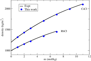
Figure 1: Density as a function of molality at T = 298.15 K and 1 bar for chloride salts aqueous solutions, RbCl and CsCl. Blue circles: this work. Solid black lines: fit of experimental data taken from RefWashburn et al. (1928). CsCl values were shifted up 200 density units for better legibility.

Next we computed the viscosity. Results are shown in Figure 2. The statistical error in the viscosities calculated in this work is always less than 5-10% (being lower at low concentrations of salt). Experimentally the viscosity of a RbCl solution does not change much with concentration, decreasing slightly at low concentrations, having a weak minimum and then increasing slightly. The simulations are not able to capture this subtle behavior. Also it is clear that the model overestimates the viscosity with respect to experimental values. However the model is able to predict that the change in the viscosity of a RbCl solution with respect to water is much smaller than that of a NaCl or KF solution at similar concentrations as will be discussed later in this paper. Further work is needed to understand the origin of this discrepancy. We checked for the possible existence of spontaneous precipitation in the simulations. However we found no evidence of precipitation at the highest concentration considered, so that this is not at the origin of the discrepancy.

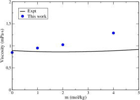
Figure 2: Shear viscosity curves as a function of concentration for aqueous RbCl solutions at 298.15 K and 1 bar. Blue circles are the results from this work. The continuous lines are the fit of experimental data taken from RefOstroff et al. (1969).

Structural properties are presented in Table 9. Before describing the structural properties of the following chloride salts, it is important to point out that the experimental data with which we compare were measured in general, at low concentrations and for this reason they depend only on the ion being studied and not on the particular salt. Regarding specifically chloride salts, it can be seen that the hydration number of the cation at high concentration is around 6. The number of CIP is below 0.5 for both salts. For RbCl the number of CIP is 0.23 at 7 m and for CsCl is 0.48 for 11 m. Thus these cations have around 6.3 (Rb⁺) or 6.6 (Cs⁺) particles around them. At high concentrations ions can replace water molecules (although due to the different sizes the replacement is not one to one). The distance at which first the peak appears for the cation-oxygen radial distribution function is slightly smaller than that found in experiments. However densities are predicted well as it can be seen in Figure 1.

Table 5: Structural properties for chloride electrolyte solutions at 298.15 K and 1 bar. Number of contact ions pairs (CIP), hydration number of cations (HN_c) and anions (HN_a), and position of the first maximum of the cation-water ($d_{c-O_{w}}$), and anion-water ($d_{a-O_{w}}$) in the radial distribution function. In parentheses, experimental data taken from the work of MarcusMarcus (1988). Properties were calculated at low concentrations and close to the solubility limit of each salt.

Salt	$m$	CIP	HNc	HNa	$d_{c-O_{w}}$	$d_{a-O_{w}}$
	(mol/kg)				Å	Å
RbCl	1	0.05	6.3(5-8)	5.8(5.3-7.2)	2.75(2.79-2.90)	3.04(3.08-3.34)
	7	0.23	6.0	5.6	2.75	3.04
CsCl	1	0.07	6.8(8-9)	5.9(5.3-7.2)	2.87(2.95-3.20)	3.04(3.08-3.34)
	11	0.48	6.0	5.5	2.85	3.04

IV.2 Fluoride salts

The densities of different fluoride salts have been calculated with the Madrid-2019-Extended force field. A comparison with experimental results is shown in Figure 3. Since the solubility of NaF is small, the results for this salt are presented separately in Figure 3a). (LiF was not considered as its solubility is extremely small, i.e 0.052 m). As can be seen the agreement with experiment for NaF is quite good. The results for KF, RbF and CsF are presented in Figure 3b). The solubilities of KF, RbF and CsF are extremely high and increase with the size of the cation. Good agreement with experiment is also found for these salts. For KF, RbF and CsF we did not find experimental results at high concentrations (even though we have evaluated the densities of these salts in the whole range of concentrations up to their solubility limit. These results are collected in the supplementary material of this work). Given the accuracy of the simulations at low-moderate concentrations, one could expect that simulations results at high concentrations should be reasonable.

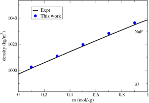
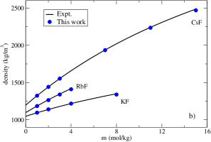
Figure 3: Density as a function of molality at T = 298.15 K and 1 bar, blue circles (this work), solid black lines (fit of experimental data taken from Ref.Pedersen et al. (1984) for NaF and KF, Ref.Washburn et al. (1928) for RbF and Ref.Novotny and Sohnel (1988) for CsF. a) NaF aqueous solutions b) KF, RbF and CsF aqueous solutions. RbF densities were shifted up 100 and CsF 200 density units for a clear visualization.

Let us now present some results for the viscosities. Since the evaluation of the viscosity is rather expensive in this work we shall evaluate the viscosity only for some selected salts. In Figure 4 the results for the viscosity of the KF are presented. It can be observed that the Madrid-2019-Extended force field of this work predicts quite well the viscosities for concentrations up to 2 m, and reasonably well for the most concentrated 5 m solution. The model overestimates somewhat the experimental value. This behavior is similar to the one found for the salts included in the original Madrid-2019 force fieldZeron et al. (2019). In Figure 4 we also present the viscosity of the JC-SPC/E model (which uses integer charges) as determined in this work. It is clear that in this case the viscosity is overestimated at 5 m by a factor of two. Thus for KF it seems that the use of scaled charges improves the description of the viscosity. To analyze if the overestimate of the viscosity of KF by the JC-SPC/E is an exception, we have also computed the viscosity of the JC-SPC/E for NaCl, which is arguably the most important salt. Somewhat surprisingly its value at room temperature and pressure and at high concentrations has not been reported before (to the best of our knowledge). The value of the viscosity of NaCl, both from the original Madrid-2019 and from the JC-SPC/E model are presented in Figure 5a). Again it is clear that the JC-SPC/E overestimates the experimental value of the viscosity of NaCl solutions at high concentrations. This is not a problem of the water model as in our previous work we showed that also the JC model of NaCl overestimates the viscosity even when used with the TIP4P/2005 model of waterZeron et al. (2019). Thus, at least for NaCl and KF it is clear that the JC-SPC/E model overestimates the value of the viscosity. This overestimation is even greater if we evaluate the ratio of the model viscosity at different concentrations to the model viscosity in pure water as we can see in Figure 5b). This is in line with the results presented by Yue and PanagiotopoulosYue and Panagiotopoulos (2019). At low concentrations it was shown that the viscosity of the JC-SPC/E increases faster than found in experiments, and that scaled and polarizable models of NaCl exhibited better (although not perfect) agreement with experiment.

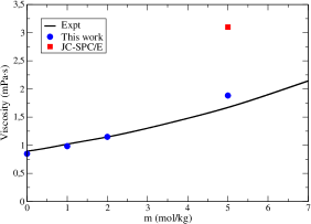
Figure 4: Shear viscosity curves as a function of concentration for aqueous KF solutions at 298.15 K and 1 bar. Blue circles are the results from this work. Red squares are the results for JC-SPC/E model and the continuous black line is the fit of experimental data taken from RefGoldsack and Franchetto (1978).

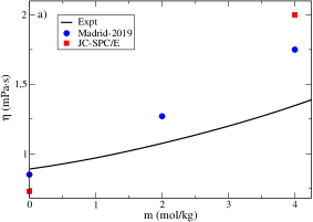
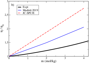
Figure 5: Viscosity as a function of concentration for NaCl solutions at 298.15 K and 1 bar. a) Shear viscosity results: Blue circles are the results from this work with original Madrid-2019 force field. Red squares are the results for JC-SPC/E model and the continuous black line is the fit of experimental data taken from refLaliberté (2007); Laliberte (2007). b) Ratio of the viscosity at different concentrations to the the viscosity in pure water. The blue solid line represents our data for Madrid-2019 model, red dashed line results for JC-SPC/E model and black solid thick line is the fit of the experimental data.

To complete the study of the fluoride salts with Madrid-2019-Extended force field we have analyzed some structural results. We have calculated the cation-anion, cation-water and anion-water radial distribution functions close to the experimental solubility limit of each salt.

Table 6: Structural properties for fluoride electrolyte solutions at 298.15 K (291.15 K for RbF) and 1 bar. Number of contact ions pairs (CIP), hydration number of cations (HN_c) and anions (HN_a), and position of the first maximum of the cation-water ($d_{c-O_{w}}$), and anion-water ($d_{a-O_{w}}$) in the radial distribution function. In parentheses, experimental data taken from the work of MarcusMarcus (1988). Properties were calculated close to the solubility limit of each salt and at low concentrations.

Salt	$m$	CIP	HNc	HNa	$d_{c-O_{w}}$	$d_{a-O_{w}}$
	(mol/kg)				Å	Å
NaF	0.1	0.00	5.5(4-8)	5.8(6-9)	2.33(2.40-2.50)	2.77(2.54-2.87)
	0.9	0.02	5.5	5.8	2.33	2.77
KF	1	0.04	5.7(6-8)	5.7(6-9)	2.73(2.60-2.80)	2.76(2.54-2.87)
	17	1.15	5.8	4.75	2.73	2.75
RbF	1	0.06	6.4(5-8)	5.7(6-9)	2.76(2.79-2.90)	2.77(2.54-2.87)
	28	2.45	4.8	3.45	2.76	2.74
CsF	1	0.05	6.9(8-9)	5.6(6-9)	2.86(2.95-3.20)	2.76(2.54-2.87)
	37	3.30	4.0	2.85	2.86	2.73

In Table 6 we have collected all the results obtained for these structural properties and we have compared them with experimental X-ray and neutron diffraction data collected in the work of MarcusMarcus (1988). As with the anion-water distances $d_{F^{-}-O_{w}}$ we see the value found in this work (around 2.75 Å) is within the experimental reported values 2.54-2.87 Å. With respect to the cation-water distance the values found in the simulations are in general slightly lower (except for K⁺) than the lower bound reported in experiments. Similar behavior was found in the Madrid-2019 for the Li⁺ cation. We do not have an explanation for this. In any case it seems that the prediction of the distance if wrong does not result in bad predictions for the densities. It can be seen that the $d_{cation-O_{w}}$ increases with the size of the cation. The difference between $d_{K^{+}-O_{w}}$ and $d_{Rb^{+}-O_{w}}$ distances are small but as expected the $d_{Rb^{+}-O_{w}}$ is larger. With respect to the hydration number one can see that the F^- anion can be hydrated by about 5.7 molecules of water (see the results for NaF which is a system without CIP). For the other salts it holds that the hydration number of the F^- anion plus the number of CIP is around six. Thus for each molecule of water removed from the hydration shell, a cation occupies its place indicating that the size of both water and K⁺, Rb⁺ and Cs⁺ cations although not identical are not so different. We have to point out that (with the exception of NaF) the rest of fluorides have very high solubility values. Moreover, in the case of RbF, at the solubility limit the total number of ions is practically equal to the number of water molecules and in the case of CsF it is even higher. Thus, we can not apply the same rules as for other salts and it is clear that one should allow higher number of CIP. It is also interesting to evaluate what a random mixing model would predict for the number of CIP. If differences in size between water and the cations are neglected, then one would expect that the number of CIP would be 6 $\cdot$ (17/55) = 1.85, 6 $\cdot$ (28/55)=3.05 and 6 $\cdot$ (37/55)=4.03 for KF, RbF and CsF respectively. Six is the number of water molecules that can be located around the F^- anion, and this is multiplied by the ratio of the molality to the number of moles of water in one kilogram. As can be seen the random mixing model would predict a number of CIP higher than found in the simulations (1.15, 2.45 and 3.30 respectively for KF, RbF and CsF). To be on the safe side we checked that no spontaneous precipitation occurred at the experimental value of the solubility limit after 50 ns using a large system with 4440 molecules of water.

We shall now present results for the bromide salts.

IV.3 Bromide salts

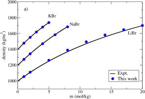
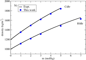
Figure 6: Density as a function of molality at T = 298.15 K and 1 bar for bromide salts aqueous solutions. a) LiBr, NaBr and KBr. b) RbBr and CsBr. Blue circles: this work. Solid black lines: fit of experimental data taken from RefWashburn et al. (1928) for all salts and RefIsono (1984) for NaBr and KBr. NaBr and CsBr densities were shifted up 200 units and KBr 400 density units for a clear visualization.

In Figure 6a) we show the results for densities of LiBr, NaBr and KBr. The solubilities of NaBr and KBr are moderate. The densities obtained for these salts are in excellent agreement with all the experimental data over all the molality range. In the case of LiBr, the simulations results overestimate slightly the experimental ones at intermediate molalities. Even though, the simulations results are very accurate. In Figure 6b) results for the densities of RbBr and CsBr salt solutions are presented. As can be seen the results of Madrid-2019-Extended are in reasonable agreement with the experimental ones. It seems that the series of the bromides is challenging. In general the agreement found is good but sometimes the density is overestimated (as in LiBr) and sometimes is underestimated (as in RbBr and CsBr).

The number of CIP have been evaluated for these salts and are presented in Table 7. NaBr at 8 m has a number of CIP of 0.24 and KBr at 5 m has a number of CIP of 0.29. Both of them follow the rule proposed by Benavides et al.Benavides et al. (2017b) with a number of CIP around or below 0.5. The same is true for RbBr and CsBr with a number of CIP of 0.58 and 0.37 respectively. Thus for these salts with solubility smaller than 10 m, the number of CIP is either around or below 0.5 at the solubility limit. However for LiBr, with a solubility of 20 m the number of CIP is 1.30.

We have also studied divalent salts for bromides. The original Madrid-2019 force field included parameters to describe the interaction between Mg²⁺ with water and between Ca²⁺ with water. Parameters for the Mg²⁺-Mg²⁺ and Ca²⁺-Ca²⁺ were also provided in our previous work. The Br^--Br^- interaction was obtained in this work from the study of 1:1 electrolytes containing Br^-. Thus for these salts we can only modify the Br^--Mg²⁺ and Br^--Ca²⁺ interactions. As can be seen in Figure 7, up to 3 m the results of the force field reproduce the experimental data. At high concentrations the results are reasonable for the model but tend to underestimate slightly the experimental results in the case of CaBr₂ and overestimate slightly them for MgBr₂. Regarding the number of contact ion pairs, for the MgBr₂ is 0 and for CaBr₂ is 0.04. Both salts have low number of CIP and do not precipitate. In this respect bromides behave like chlorides. Both Mg²⁺ and Ca²⁺ have a strong interaction with water, and cation-anion contact are rare.

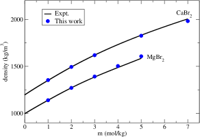
Figure 7: Density as a function of molality at T = 298.15 K and 1 bar for bromide salts 1:2 aqueous solutions, MgBr₂ and CaBr₂. Blue circles: this work. Solid black lines: fit of experimental data taken from RefWashburn et al. (1928) and RefNovotny and Sohnel (1988). CaBr₂ values were shifted up 200 density units for better legibility.

Let us now study the behavior of the viscosities for the bromide salts. In particular we shall analyze LiBr, NaBr, KBr and MgBr₂. Results are shown in Figure 8. It is interesting that experimentally, LiBr, NaBr and KBr have a small impact on the viscosity of water (increasing it slightly in the case of NaBr and LiBr) and decreasing it slightly in the case of KBr. The Madrid-2019-Extended force field is able to capture this effect. Although the agreement with experiment is not quantitative the trends are described quite well. However adding MgBr₂ significantly increases the viscosity of water. Again this effect is captured by the force field but it seems that the model overestimates the magnitude of the effect (and the deviation is already visible at 2 m). This is similar to the behavior found for MgCl₂. For these salts, MgCl₂ and MgBr₂, the scaled charges do a good job in describing the experimental values of the viscosities but tend to overestimate their values.

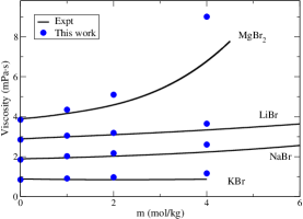
Figure 8: Shear viscosity curves as a function of concentration for aqueous bromides solutions at 298.15 K and 1 bar. Blue circles are the results from this work. The continuous lines are the fit of experimental data taken from RefsGoldsack and Franchetto (1978); Zaitsev and Aseev (1992); Lo Surdo and Wirth (1979). NaBr, LiBr and MgBr₂ values were shifted up 1, 2 and 3 viscosity units respectively for better legibility.

We shall now present the results for the structural properties. The hydration number of the bromide anion is around 6. Except for LiBr, for the rest of salts the sum of the hydration number and the number of CIP is around 6. That makes sense when taking into account that Na⁺, K⁺, Rb⁺ and Cs⁺ have sizes similar to that of water. However the exception is LiBr. For this salt, at 20 m one has 7.5 molecules around the Br^- anion, 6.3 water and 1.5 Li⁺. Thus Li⁺ when in the first coordination of Br^-, provokes a contraction of the molecules of water hydrating the bromide anion. The bromide-water distance found in this work is within the range of values reported in experiments. For the cations again, the cation-water distance found in the simulation is always slightly below the value reported in experiments. We do not have an explanation for this finding, especially taking into account that the predictions of the densities for bromide salts is quite reasonable.

Table 7: Structural properties for bromide electrolyte solutions at 298.15 K and 1 bar. Number of contact ions pairs (CIP), hydration number of cations (HN_c) and anions (HN_a), and position of the first maximum of the cation-water ($d_{c-O_{w}}$), and anion-water ($d_{a-O_{w}}$) in the radial distribution function. In parentheses, experimental data taken from the work of MarcusMarcus (1988). Properties were calculated at low concentrations and close to the solubility limit of each salt.

Salt	$m$	CIP	HNc	HNa	$d_{c-O_{w}}$	$d_{a-O_{w}}$
	(mol/kg)				Å	Å
LiBr	1	0.18	3.8(3.3-5.3)	6.3(4-6)	1.84(1.90-2.25)	3.15(3.01-3.45)
	20	1.5	2.0	5.6	1.84	3.15
NaBr	1	0.02	5.5(4-8)	6.0(4-6)	2.34(2.40-2.50)	3.15(3.01-3.45)
	8	0.24	5.3	6.0	2.33	3.15
KBr	1	0.04	6.7(6-8)	5.9(4-6)	2.73(2.60-2.80)	3.15(3.01-3.45)
	5	0.29	6.4	5.8	2.73	3.15
RbBr	1	0.10	6.3(5-8)	5.8(4-6)	2.76(2.79-2.90)	3.15(3.01-3.45)
	7	0.58	5.8	5.4	2.75	3.15
CsBr	1	0.08	6.7(8-9)	5.9(4-6)	2.85(2.95-3.20)	3.15(3.01-3.45)
	5	0.37	6.2	5.6	2.85	3.15
MgBr2	1	0.00	6.0(6-8.1)	5.9(4-6)	1.92(2.00-2.11)	3.15(3.01-3.45)
	5	0.00	6.0	5.9	1.92	3.15
CaBr2	1	0.00	7.4(5.5-8.2)	6.1(4-6)	2.38(2.39-2.46)	3.15(3.01-3.45)
	7	0.04	6.9	6.1	2.38	3.15

Finally in Figure 9 we show the cation-water radial distribution function as obtained in this work for a 1 m solution of LiBr, NaBr, KBr, RbBr and CsBr. It can be seen that the distance at which the first peak occurs increases with the size of the cation. The increase is clear for all the cations with one exception. The K⁺-O_w and Rb⁺-O_w have a similar location of the first peak (i.e 2.73 vs 2.75 Å  respectively).

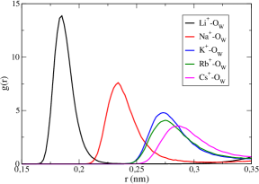
Figure 9: Cation-water oxygen radial distribution function for bromide solutions at 298.15 K, 1 bar, and 1 m as were obtained with the Madrid-2019-Extended model in solutions: LiBr, NaBr, KBr, RbBr and CsBr

IV.4 Iodine salts

We present now the properties for the iodine salts. In particular we shall consider LiI, NaI, KI, RbI, CsI, MgI₂ and CaI₂. Thus for iodine salts we present results for a number of cations, including monovalent and divalent cations. We shall start by presenting densities for monovalent ions as obtained from the Madrid-2019-Extended. Results for LiI, NaI and KI are shown in Figure 10a), and results for RbI and CsI in Figure 10b).

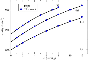
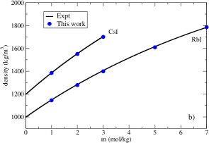
Figure 10: Density as a function of molality at T = 298.15 K and 1 bar for iodide salts aqueous solutions. a) LiI, NaI and KI. b) and RbI and CsI. Blue circles: this work. Solid black lines: fit of experimental data taken from RefWashburn et al. (1928). NaI and CsI densities were shifted up 200 and KI 400 density units for better legibility.

LiI, NaI and KI simulation results are in excellent agreement with the experimental ones for the whole range of molalities. However, at the highest molalities studied for each salt (8 m for KI and 12 m for NaI and LiI) the simulation results overestimate slightly the experimental values. The results for RbI and CsI aqueous solutions are shown in Figure 10b). The results for both salts are in excellent agreement with experiment for all concentrations.

We shall now turn to salts containing divalent cations. Figure 11 shows the results for the densities of divalent salts of iodide. Results for CaI₂ are in excellent agreement with experimental data over all the molality range. On the other hand, results for MgI₂ overestimate the experimental values at high molalities.

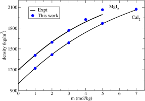
Figure 11: Density as a function of molality at T = 298.15 K and 1 bar for iodide salts 1:2 aqueous solutions, MgI₂ and CaI₂. Blue circles: this work. Solid black lines: fit of experimental data taken from RefWashburn et al. (1928). MgI₂ values were shifted up 200 units for better legibility.

Figure 12 shows the viscosities obtained with Madrid-2019-Extended force field for NaI and CsI. The agreement is not perfect, but still reasonable. The case of CsI is special because in experiments the viscosity decreases slightly as the salt concentration increases. The model is not able to capture this decrease in viscosity but at least the increase that occurs is very small. The case of NaI is similar to the other salts studied in this work and in Madrid-2019Zeron et al. (2019) force field. The viscosities are well predicted for concentrations up to 1-2 m and overestimated afterwards. The overestimation is not dramatic but seems to a systematic deviation found in the Madrid-2019-Extended force field. Very little is known about the behavior of the viscosities at high concentrations for most of the force fields of ionic systems. The study of Yue and PanagiotopoulosYue and Panagiotopoulos (2019) and the results for KF and NaCl presented before seems to suggest that integer charges deviate typically more from experiment than scaled charges. It is also clear that scaled charges improve the description but are not able to obtain a full quantitative agreement with experiment. Notice that the deviations are not due to an incorrect prediction of densities. The Madrid-2019-Extended force field yields good prediction of the experimental densities. Therefore, the deviations are due to some missing physics in the model.

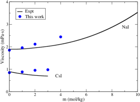
Figure 12: Shear viscosity curves as a function of concentration for aqueous NaI and CsI solutions at 298.15 K and 1 bar. Blue circles are the results from this work. The continuous lines are the fit of experimental data taken from RefsAbdulagatov et al. (2006); Laliberte (2007) for NaI and RefJones and Fornwalt (1936) for CsI. NaI values were shifted up 1 viscosity unit for better legibility.

Structural properties for iodine salts are presented in Table 8. The hydration number of iodine is about 6.1 (although this number changes from one salt to another at the high concentrations considered in Table 8). The number of CIP is almost zero for Li⁺, Mg²⁺ and Ca⁺, thus reflecting that these ions are strongly hydrated and CIP are rare. For the rest of the salts the number of CIP is typically below 0.5 at the solubility limit. The main exception to this rule is the NaI with a higher number of CIP.

Table 8: Structural properties for iodine electrolyte solutions at 298.15 K and 1 bar. Number of contact ions pairs (CIP), hydration number of cations (HN_c) and anions (HN_a), and position of the first maximum of the cation-water ($d_{c-O_{w}}$), and anion-water ($d_{a-O_{w}}$) in the radial distribution function. In parentheses, experimental data taken from the work of MarcusMarcus (1988). Properties were calculated at low concentrations and close to the solubility limit of each salt.

Salt	$m$	CIP	HNc	HNa	d${}_{c-O_{w}}$	d${}_{a-O_{w}}$
	(mol/kg)				Å	Å
LiI	1	0.00	4.0(3.3-5.3)	6.1(4-6)	1.84(1.90-2.25)	3.28(3.01-3.45)
	12	0.01	4.0	6.1	1.84	3.28
NaI	1	0.01	5.5(4-8)	6.1(4-6)	2.33(2.40-2.50)	3.28(3.01-3.45)
	12	1.12	5.3	6.1	2.33	3.28
KI	1	0.03	6.5(6-8)	6.0(4-6)	2.72(2.60-2.80)	3.29(3.01-3.45)
	8	0.30	6.2	6.1	2.72	3.28
RbI	1	0.10	6.3(5-8)	6.0(5.3-7.2)	2.75(2.79-2.90)	3.29(3.08-3.34)
	7	0.60	5.8	5.5	2.75	3.28
CsI	1	0.10	6.6(8-9)	6.0(5.3-7.2)	2.86(2.95-3.20)	3.28(3.08-3.34)
	3	0.35	6.4	5.9	2.86	3.28
MgI2	1	0.00	6.0(6-8.1)	6.1(4-6)	1.92(2.00-2.11)	3.28(3.01-3.45)
	5	0.00	6.0	6.1	1.92	3.28
CaI2	1	0.00	7.4(5.5-8.2)	6.0(4-6)	2.38(2.39-2.46)	3.28(3.01-3.45)
	7	0.00	6.9	6.6	2.38	3.28

To finish this section we shall present results for the anion-oxygen radial distribution function for F^-, Cl^-, Br^- and I^-. Figure 13 shows the anion-water oxygen radial distribution functions for 1 m sodium salts solutions with the different anions developed in Madrid-2019 and Madrid-2019-Extended force fields. It can be seen that the anion-oxygen distance increases with the size of the anion.

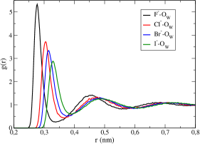
Figure 13: Anion-water oxygen radial distribution functions for sodium solutions at 298.15 K, 1 bar, and 1 m as were obtained with the Madrid-2019-Extended model in solutions: NaF (0.9 m), NaCl, NaBr and NaI.

IV.5 Sulfate salts

We shall finish by presenting properties for the sulfate salts. We have included the Rb₂SO₄ and Cs₂SO₄. The results for the densities are in excellent agreement with experimental results as we show in Figure 14. Regarding the structural properties we can observe similar results than those obtained for the sulfate salts studied in the Madrid-2019 force field. The number of contact ion pairs is higher than for other salts (sulfate group is a huge ion) and the hydration numbers are higher than the experimental ones. In our opinion, the results obtained by using simulations are more realistic than the ones from experiments because the size of the sulfate group is too big to have only 8 molecules of water around.

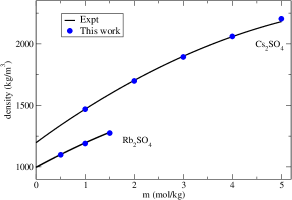
Figure 14: Density as a function of molality at T = 298.15 K and 1 bar for sulfate salts aqueous solutions, Rb₂SO₄ and Cs₂SO₄. Blue circles: this work. Solid black lines: fit of experimental data taken from RefsWashburn et al. (1928); Ludlum and Warner (1965); Sun et al. (2021). Cs₂SO₄ values were shifted up 200 density units for better legibility.

Table 9: Structural properties for sulfate electrolyte solutions at 298.15 K and 1 bar. Number of contact ions pairs (CIP), hydration number of cations (HN_c) and anions (HN_a), and position of the first maximum of the cation-water ($d_{c-O_{w}}$), and anion-water ($d_{a-O_{w}}$) in the radial distribution function. In parentheses, experimental data taken from the work of MarcusMarcus (1988). Properties were calculated at low concentrations and close to the solubility limit of each salt.

Salt	$m$	CIP	HNc	HNa	$d_{c-O_{w}}$	$d_{S-O_{w}}$	$d_{O_{s}-O_{w}}$
	(mol/kg)				Å	Å	Å
Rb2SO4	0.5	0.35	6.2(5-8)	12.5(6.4-8.1)	2.75(2.79-2.90)	3.76(3.67-3.89)	3.02(2.84-2.95)
	1.5	0.70	6.0	11.7	2.75	3.77	3.02
Cs2SO4	1	0.45	6.5(8-9)	12(6.4-8.1)	2.86(2.95-3.20)	3.78(3.67-3.89)	3.02(2.84-2.95)
	5	1.25	5.8	10.2	2.85	3.76	3.02

IV.6 Density of molten salts

Although the main purpose of using scaled charges is to improve the description of the aqueous solution we shall now present results obtained for the molten salts (at room pressure and at the experimental melting temperature).

In table 10 we have collected the results for the density of the molten salts. As we pointed out in the Madrid-2019 force field, the use of scaled charges improves the description of the aqueous electrolyte solutions but at the cost of correctly describing the properties of the solid and of the melt. In Table 10 we can see that the results obtained for the densities of the melt with scaled charges are about 20 or even 25 $\%$ below the experimental molten densities. When we use a unit charge (with the same parameters as for 0.85 charge) the results are similar to the experimental ones. It is interesting to mention that we have adjusted the cation-anion and anion-anion interactions using the results for the densities of the melt. These interactions have almost no effect in aqueous solution where by far the most important interactions are cation-oxygen and anion-oxygen. However the parameters of the cation-anion interactions were determined having two properties in mind, namely the density of the melt and a reasonable number of CIP at the experimental value of the solubility limit. It should be mentioned that in the simulations we found problems for LiF and LiBr in getting a stable melt at the experimental conditions. In the case of LiF we found spontaneous precipitation, and for LiBr spontaneous cavitation (due to the formation of chains of ions). For these two salts our reported simulation were obtained at 200 K above the experimental melting temperature for LiF and 3000 bar at the experimental melting temperature for LiBr (at 1 bar a 7-8 $\%$ lower density is expected taking into account the experimental behavior of other molten salts)Goldmann and Todheide (1976).

Table 10: Densities of the molten salts (at 1 bar and the experimental melting temperatureHaynes (2011)). Values of this work are given under columns labelled $q_{sc}$ and $q$ which are obtained using scaled charges ($\pm$0.85 Z $e$) and integer charges ($\pm$1.0 Z $e$) for the ions, respectively. For LiF the simulations results were obtained at 200 K above the experimental melting temperature. For LiBr the simulation results were obtained at 3000 bar.

Salt	Melt density
	kg/m3
	Expt	$q_{sc}$	$q$
LiF	1810	1231	1570
LiBr	2528	2220	2445
LiI	3109	2600	3087
NaF	1948	1524	1949
NaBr	2342	1954	2429
NaI	2742	2166	2685
KF	1910	1327	1708
KBr	2127	1634	2090
KI	2448	1825	2325
RbF	2870	2260	2869
RbCl	2248	1547	1986
RbBr	2715	2150	2715
RbI	2904	2279	2876
CsF	3649	2864	3653
CsCl	2790	1989	2568
CsBr	3133	2357	3036
CsI	3197	2479	3191
MgBr2	2620	2305	2555
MgI2	3050	2693	3004
CaBr2	3111	2485	3017
CaI2	3443	2766	3335

IV.7 Self diffusion coefficient of ions at infinite dilution

Let us finish by presenting results for the diffusion coefficient of the ions at infinite dilution. We have performed molecular dynamics simulations of systems with 5550 water molecules and 1 ion in order to study the self diffusion coefficient of the ion at infinite dilution. The fact that we are using only one ion (we have denoted that as single ion) implies that the system is not electroneutral (although technically the use of Ewald sums implies that one has a neutralizing diffuse background of opposite charge). This is standard practice done to compute diffusion coefficients at infinite dilution. However, to check for the possible existence of artefacts we also simulated an electroneutral system having 5550 water molecules, 1 Na⁺ and 1 Cl^- corresponding to a molality of 0.01 m and we obtained quite similar results to those obtained with single ion simulations. Thus, we have used the single ion method in the rest of the ions. All the results collected in Table 11 and presented in Figure 15 are the result of the average of 5 independent runs of 40 ns with 5550 water molecules and 1 ion. So that, each point obtained is the result of 200 ns of simulation, 2.8 $\mu$s in total. For the Madrid-2019 model we have also included in Table 11 the results obtained by Dopke et $al.$Dopke et al. (2020), obtaining good agreement except for Cl^- where we obtained an slightly larger value (although still within the combined uncertainty). Notice that the results of Dopke et $al.$ were obtained using a smaller system having 523 molecules of water.

Table 11: Diffusion coefficients of the Madrid-2019 ions (in cm²/s) at 1 bar and 298.15 K. We present the results obtained in this work, the results of Dopke et $al.$ Dopke et al. (2020). The experimental values are from Haynes (2011). The results are obtained from the average of five independent simulations and we have applied the hydrodynamic corrections of Yeh and HummerYeh and Hummer (2004).

Ion		$D_{exp}$$\cdot$105	$D_{this\;work}$$\cdot$105	$D_{this\;work}$$\cdot$105	$D_{Dopke}$$\cdot$105
			Single Ion	Electroneutral
Na+		1.334	1.36(07)	1.39(11)	1.28(15)
Cl-		2.03	1.76(09)	1.75(08)	1.60(08)
K+		1.957	1.90(11)	-	1.93(06)
Li+		1.029	1.07(09)	-	1.08(02)
Mg2+		0.706	0.82(07)	-	0.87(13)
Ca2+		0.792	0.84(04)	-	0.89(08)
SO42-		1.065	1.27(05)	-	-
F-		1.475	1.36(4)	-	-
Br-		2.080	1.68(5)	-	-
I-		2.045	1.71(6)	-	-
Rb+		2.072	1.88(5)	-	-
Cs+		2.056	1.99(6)	-	-

Figure 15a) shows that the results for most of the cations (with the exception of Rb⁺) are in excellent agreement with experimental results. It can also be seen that for monovalent cations the diffusion coefficient increases as the water-cation distance increases. For divalent cations, on the other hand, there is no major change in the diffusion coefficient with increasing water-cation distance. In the case of the anions (in particular for halogens) the results obtained are below the experimental ones with the exception of the sulfate in which the opposite is true as we can see in Figure 15b). In this case the diffusion coefficient increases from fluorine anion to chlorine anion and remains constant thereafter. Notice that we have applied the hydrodynamic corrections of Yeh and HummerYeh and Hummer (2004). using the viscosiy of the TIP4P/2005 water model. We have considered that the viscosity of the systema it is not affected by the dilution of 1 single ion (i.e. at infinite dilution.

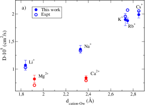
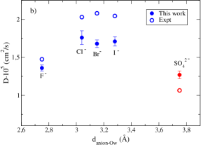
Figure 15: Diffusion coefficients of the Madrid-2019 ions at 1 bar and 298.15 K (full circles) compared with experimental valuesHaynes (2011) (empty circles) in function of the position of the first maximum of the cation-water ($d_{cation-O_{w}}$), and anion-water ($d_{anion-O_{w}}$) in the radial distribution function. a) Results for cations. In blue monovalent cations, in red, divalent cations. b) Results for anions. In blue monovalent anions, in red, sulfate anions.

IV.8 Diffusion coefficient of water for several salts: Stokes-Einstein relation for aqueous electrolytes

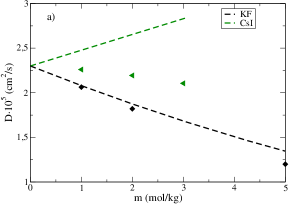
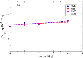
Figure 16: a) Diffusion coefficients of water for several salts of the Madrid-2019-Extended at 1 bar and 298.15 K. Green triangles are the results for CsI and black squares for KF. b)Product of the water diffusion coefficient and viscosity in function of molality for different salts of the Madrid-2019-Extended model: Blue circles are the results for NaBr, red squares for NaI and pink triangles for RbCl. Experimental results are plotted in dashed lines in the same colors as their respective salts. Experimental diffusion coefficients obtained from RefMüller and Hertz (1996).

In this work we have also considered it relevant to analyse the water diffusion coefficients for various aqueous solutions of electrolytes at different concentrations. The salts chosen have been some of those for which we have calculated the viscosity. This is due to the fact that when applying the Yeh and Hummer correctionsYeh and Hummer (2004), the viscosity used was that of the model. As can be seen in Figure 16a, the force field, in the case of KF, is able to reproduce the experimental results accurately (it was the salt that best reproduced the viscosities). Nevertheless, in the case of CsI we have the same problem that other authors pointed out Kim et al. (2012). Diffusion coefficient of water in CsI aqueous solutions increases with the concentration. This behaviour is anomalous and molecular dynamics simulations are not able (even using scaled charges). For CsI the model is able to capture at least a very small impact of the salt in the diffussion coefficient of water. It is true that Ding et al.Ding et al. (2014) showed that with ab initio calculations it is possible to reproduce this trend. We have also calculated the diffusion coefficients of water in the presence of other three salts in order to evaluate if the product of the viscosity and the diffusion coefficient of water remains constant (i.e. if the Stokes-Einstein relationDill et al. (2003) is satisfied). In Figure 16b we have plotted the values of the product of the water diffusion coefficient and viscosity obtained in this work versus salt concentration. It can be seen how the all the results follow the same trend and all salts keep the $D\cdot\eta$ product almost constant with a slightly increase with the concentration. The experimental results (dashed lines) show the same trend. The agreement between experimental and simulation results for the product $D\cdot\eta$ is excellent. Of course, just because the model reproduces the experimental results of the product $D\cdot\eta$ does not mean that it reproduces the experimental values of viscosity and diffusion coefficients. What happens is that when the force field overestimates the experimental viscosity, to keep constant the product (and reproduce experimental results), the model must underestimate the diffusion coefficients of the water.

V Concluding remarks

In this work we have developed the Madrid-2019-Extended force field for electrolytes in water (as described by the TIP4P/2005 model). This force field extends the Madrid-2019 force field to the cations Rb⁺ and Cs⁺ and to the anions F^-, Br^- and I^-. Thus, the Madrid-2019-Extended force field includes the ions considered in the celebrated Joung-Cheatham force field, and some additional ions such as Mg²⁺ and Ca²⁺. We have presented results for the densities of a number of salts, and of the viscosities for some selected salts. Hydration numbers, radial distribution functions, and contact ion pairs were also calculated as well as diffusion coefficients of the ions at infinite dilution. The main conclusions of this work are as follows:

• The use of scaled charges allows us to describe accurately the densities of a large number of salts as was already the case with the Madrid-2019 force field.

• As we have pointed out in the Madrid-2019 force field, the use of scaled charges improves the description of aqueous solutions but the cost is the description of solid phases: densities for molten salts are underestimated by about a 20$\%$

• Following the philosophy of the Madrid-2019 force field the charge 0.85 Z $e$ describes quite well the viscosities for concentrations up to 2 m. However, at higher molalities there are large deviations, especially for divalent salts.

• Self diffusion coefficients at infinite dilution are described accurately for most of the cations but not for the anions, whose results are slightly worse.

• No spontaneous precipitation was found when performing simulations at the experimental value of the solubility limit.

• The number of CIP was in general below 0.5 for salts with solubility smaller than 10 m. For salts with huge solubility this rule can not be applied. For these salts the number of CIP was smaller by about a factor of between 0.6-0.8 of that found from the random mixing rule, thus illustrating that water is a good solvent for the ions.

To summarize, the combination of a good model of water and scaled charges yields a reasonable description of electrolyte solutions improving unit charges force fields results. The Madrid-2019-Extended should be regarded as a computationally cheap way of introducing some degree of polarization. The model provides reasonable results but for certain properties the agreement with experiment is not quantitative thus showing the limits of this approach. In the particular case of transport properties it is clear that there is room for improvement. One could argue that polarizable models should improve the description. Time is needed to provide evidence of that. Also, the impact of nuclear quantum effects in transport properties of electrolytes has not been considered in detail in the literature. For the time being we hope that the Madrid-2019-Extended, with care, could be useful to provide some predictions regarding interesting physical problems. In the future it will be useful to study the performance of the Madrid-2019 force field in a number of problems such as solubilities, freezing point depression, nucleation of ice in salty solutions and electrical conductivity. A face to face comparison with force fields that use integer charges will bring more evidence of the benefits and drawbacks of using scaled charges.

VI Supplementary

In the supplementary material we have collected the numerical results for densities and viscosities obtained in this work for several salt solutions and the complete set of parameters for the force field Madrid-2019 and its extended version. See also topol.top file of GROMACS with the force field Madrid-2019 and its extended version attached with this paper.

Conflict of interest

The authors declare that there are no conflicts of interest.

Data Availability

The data that support the findings of this work are available within the article and its supplementary material.

References

- Debye and Hückel (1923) P. Debye and E. Hückel, Physikalische Zeitschrift 24, 185 (1923).
- Sangster and Dixon (1976) M. Sangster and M. Dixon, Adv. Phys. 25, 247 (1976).
- Adams et al. (1977) M. E. Adams, I. R. McDonald, and K. Singer, Proc. R. Soc. Lond. A 357, 37 (1977).
- Heinzinger and Vogel (1974) K. Heinzinger and P. Vogel, Z. Naturforsch sect. A 29, 1164 (1974).
- Vogel and Heinzinger (1975) P. Vogel and K. Heinzinger, Z. Naturforsch sect. A 30, 789 (1975).
- Heinzinger and Vogel (1976) K. Heinzinger and P. Vogel, Z. Naturforsch sect. A 31, 463 (1976).
- Jorgensen et al. (1983) W. L. Jorgensen, J. Chandrasekhar, J. D. Madura, R. W. Impey, and M. L. Klein, J. Chem. Phys. 79, 926 (1983).
- Berendsen et al. (1987) H. J. C. Berendsen, J. R. Grigera, and T. P. Straatsma, J. Phys. Chem. 91, 6269 (1987).
- Horn et al. (2004) H. W. Horn, W. C. Swope, J. W. Pitera, J. D. Madura, T. J. Dick, G. L. Hura, and T. Head-Gordon, J. Chem. Phys. 120, 9665 (2004).
- Mahoney and Jorgensen (2001) M. Mahoney and W. L. Jorgensen, J. Chem. Phys. 115, 10758 (2001).
- Abascal and Vega (2005) J. L. F. Abascal and C. Vega, J. Chem. Phys. 123, 234505 (2005).
- Vega and Abascal (2011) C. Vega and J. L. F. Abascal, Phys. Chem. Chem. Phys 13, 19663 (2011).
- Vega et al. (2009) C. Vega, J. L. F. Abascal, M. M. Conde, and J. L. Aragones, Faraday Discuss. 141, 251 (2009).
- Smith et al. (2018) W. R. Smith, I. Nezbeda, J. Kolafa, and F. Moučka, Fluid Phase Equilib. 466, 19 (2018).
- Chandrasekhar et al. (1984) J. Chandrasekhar, D. C. Spellmeyer, and W. L. Jorgensen, J. Am. Chem. Soc. 106, 903 (1984).
- Straatsma and Berendsen (1988) T. Straatsma and H. Berendsen, J. Chem. Phys. 89, 5876 (1988).
- Aqvist (1990) J. Aqvist, J. Phys. Chem. 94, 8021 (1990).
- Dang (1992) L. X. Dang, J. Chem. Phys. 96, 6970 (1992).
- Beglov and Roux (1994) D. Beglov and B. Roux, J. Chem. Phys. 100, 9050 (1994).
- Smith and Dang (1994) D. E. Smith and L. X. Dang, J. Chem. Phys. 100, 3757 (1994).
- Roux (1996) B. Roux, Biophys. J. 71, 3177 (1996).
- Peng et al. (1997) Z. Peng, C. S. Ewig, M.-J. Hwang, M. Waldman, and A. T. Hagler, J. Phys. Chem. A 101, 7243 (1997).
- Weerasinghe and Smith (2003) S. Weerasinghe and P. E. Smith, J. Chem. Phys. 119, 11342 (2003).
- Jensen and Jorgensen (2006) K. P. Jensen and W. L. Jorgensen, J. Chem. Theory Comput. 2, 1499 (2006).
- Lamoureux and Roux (2006) G. Lamoureux and B. Roux, J. Phys. Chem. B 110, 3308 (2006).
- Alejandre and Hansen (2007) J. Alejandre and J.-P. Hansen, Phys. Rev. E 76, 061505 (2007).
- Lenart et al. (2007) P. J. Lenart, A. Jusufi, and A. Z. Panagiotopoulos, J. Chem. Phys. 126, 044509 (2007).
- Joung and Cheatham (2008) I. S. Joung and T. E. Cheatham, J. Phys. Chem. B 112, 9020 (2008).
- Corradini et al. (2010) D. Corradini, M. Rovere, and P. Gallo, J. Chem. Phys. 132, 134508 (2010).
- Callahan et al. (2010) K. M. Callahan, N. N. Casillas-Ituarte, M. Roeselová, H. C. Allen, and D. J. Tobias, J. Phys. Chem. A 114, 5141 (2010).
- Yu et al. (2010) H. Yu, T. W. Whitfield, E. Harder, G. Lamoureux, I. Vorobyov, V. M. Anisimov, A. D. MacKerell Jr, and B. Roux, J. Chem. Theory Comput. 6, 774 (2010).
- Reif and Hünenberger (2011) M. M. Reif and P. H. Hünenberger, J. Chem. Phys. 134, 144104 (2011).
- Gee et al. (2011) M. B. Gee, N. R. Cox, Y. Jiao, N. Bentenitis, S. Weerasinghe, and P. E. Smith, J. Chem. Theory Comput. 7, 1369 (2011).
- Deublein et al. (2012) S. Deublein, J. Vrabec, and H. Hasse, J. Chem. Phys. 136, 084501 (2012).
- Mao and Pappu (2012) A. H. Mao and R. V. Pappu, J. Chem. Phys. 137, 064104 (2012).
- Mamatkulov et al. (2013) S. Mamatkulov, M. Fyta, and R. R. Netz, J. Chem. Phys. 138, 024505 (2013).
- Moučka et al. (2013a) F. Moučka, I. Nezbeda, and W. R. Smith, J. Chem. Theory Comput. 9, 5076 (2013a).
- Kiss and Baranyai (2014) P. T. Kiss and A. Baranyai, J. Chem. Phys. 141, 114501 (2014).
- Kolafa (2016) J. Kolafa, J. Chem. Phys. 145, 204509 (2016).
- Elfgen et al. (2016) R. Elfgen, M. Hülsmann, A. Krämer, T. Köddermann, K. N. Kirschner, and D. Reith, Eur. Phys. J. Spec. Top. 225, 1391 (2016).
- Pethes (2017) I. Pethes, J. Mol. Liq. 242, 845 (2017).
- Yagasaki et al. (2020) T. Yagasaki, M. Matsumoto, and H. Tanaka, J. Chem. Theory Comput. 16, 2460 (2020).
- Dopke et al. (2020) M. F. Dopke, O. A. Moultos, and R. Hartkamp, J. Chem. Phys. 152, 024501 (2020).
- Benavides et al. (2016) A. L. Benavides, J. L. Aragones, and C. Vega, J. Chem. Phys. 144, 124504 (2016).
- Benavides et al. (2017a) A. L. Benavides, M. A. Portillo, V. C. Chamorro, J. R. Espinosa, J. L. F. Abascal, and C. Vega, J. Chem. Phys. 147, 104501 (2017a).
- Zeron et al. (2019) I. M. Zeron, J. L. F. Abascal, and C. Vega, J. Chem. Phys. 151, 134504 (2019).
- Zeron et al. (2021) I. M. Zeron, M. A. Gonzalez, E. Errani, C. Vega, and J. L. F. Abascal, J. Chem. Theory Comput. 17, 1715 (2021).
- Kim et al. (2012) J. S. Kim, Z. Wu, A. R. Morrow, A. Yethiraj, and A. Yethiraj, J. Phys. Chem. B 116, 12007 (2012).