Obtaining the pseudoinverse solution of singular range-symmetric linear systems with GMRES-type methods

Abstract

It is well known that for singular inconsistent range-symmetric linear systems, the generalized minimal residual (GMRES) method determines a least squares solution without breakdown. The reached least squares solution may be or not be the pseudoinverse solution. We show that a lift strategy can be used to obtain the pseudoinverse solution. In addition, we propose a new iterative method named RSMAR (minimum $\mathbf{A}$-residual) for range-symmetric linear systems $\mathbf{A}\mathbf{x}=\mathbf{b}$. At step $k$ RSMAR minimizes $\|\mathbf{A}\mathbf{r}_{k}\|$ in the $k$th Krylov subspace generated with $\{\mathbf{A},\mathbf{r}_{0}\}$ rather than $\|\mathbf{r}_{k}\|$, where $\mathbf{r}_{k}$ is the $k$th residual vector and $\|\cdot\|$ denotes the Euclidean vector norm. We show that RSMAR and GMRES terminate with the same least squares solution when applied to range-symmetric linear systems. We provide two implementations for RSMAR. Our numerical experiments show that RSMAR is the most suitable method among GMRES-type methods for singular inconsistent range-symmetric linear systems.

Keywords. GMRES, RRGMRES, RSMAR, DGMRES, MINRES, MINRES-QLP, MINARES, singular range-symmetric linear systems, pseudoinverse solution, lifting strategy

2020 Mathematics Subject Classification: 15A06, 15A09, 65F10, 65F25, 65F50

1 Introduction

We consider the linear system of equations

$$\mathbf{A}\mathbf{x}=\mathbf{b},$$ (1)

where $\mathbf{b}\in\mathbb{R}^{n}$ is a vector, and $\mathbf{A}\in\mathbb{R}^{n\times n}$ is a large singular range-symmetric (i.e., ${\rm range}(\mathbf{A})={\rm range}(\mathbf{A}^{\top})$) matrix for which matrix-vector products $\mathbf{A}\mathbf{v}$ can be computed efficiently for any vector $\mathbf{v}\in\mathbb{R}^{n}$. For any $\mathbf{b}\in\mathbb{R}^{n}$, we seek the unique solution $\mathbf{x}_{\star}$ that solves the problem

$$\min{\|\mathbf{x}\|}\qquad\mbox{subject to}\qquad\mathbf{A}^{\top}\mathbf{A}\mathbf{x}=\mathbf{A}^{\top}\mathbf{b}.$$ (2)

It is clear that $\mathbf{x}_{\star}$ is the unique minimum Euclidean norm solution to (1) if $\mathbf{b}\in{\rm range}(\mathbf{A})$ and the unique minimum Euclidean norm least squares solution otherwise. Here we call $\mathbf{x}_{\star}$ the pseudoinvese solution of (1).

If system (1) is consistent (i.e., $\mathbf{b}\in{\rm range}(\mathbf{A})$), then the GMRES method by Saad and Schulz [30] determines the pseudoinvese solution without breakdown. If system (1) is inconsistent (i.e., $\mathbf{b}\notin{\rm range}(\mathbf{A})$), then GMRES determines a least squares solution without breakdown, and the reached least squares solution may be or not be the pseudoinverse solution. We refer to [4, section 2] for the above statements. Applicable solvers for the pseudoinverse solution of (1) with arbitrary $\mathbf{b}\in\mathbb{R}^{n}$ would be the RRGMRES method by Calvetti, Lewis, and Reichel [5] and the DGMRES method by Sidi [32]. Let $\mathbf{x}_{k}$ be an approximate solution to $\mathbf{x}_{\star}$ with residual $\mathbf{r}_{k}=\mathbf{b}-\mathbf{A}\mathbf{x}_{k}$. Assume that $\mathbf{x}_{0}=\mathbf{0}$. At step $k$, GMRES minimizes $\|\mathbf{r}_{k}\|$ over the $k$th Krylov subspace

$$\mathcal{K}_{k}(\mathbf{A},\mathbf{b}):={\rm span}\{\mathbf{b},\mathbf{A}\mathbf{b},\ldots,\mathbf{A}^{k-1}\mathbf{b}\},$$

RRGMRES minimizes $\|\mathbf{r}_{k}\|$ over the $k$th Krylov subspace $\mathcal{K}_{k}(\mathbf{A},\mathbf{A}\mathbf{b})$ (which belongs to ${\rm range}(\mathbf{A})$ and thus is called range-restricted), and DGMRES minimizes $\|\mathbf{A}^{\alpha}\mathbf{r}_{k}\|$ over $\mathcal{K}_{k}(\mathbf{A},\mathbf{A}\mathbf{b})$. Here, $\alpha$ is the index of $\mathbf{A}$, the size of a largest Jordan block associated with zero eigenvalue. If $\mathbf{A}$ is range-symmetric, then $\alpha=1$ (see section 2).

When $\mathbf{A}$ is symmetric, GMRES is theoretically equivalent to MINRES [28]. Hence, MINRES determines the pseudoinverse solution if $\mathbf{b}\in{\rm range}(\mathbf{A})$ and a least squares solution (but not necessarily the pseudoinverse solution) otherwise. MINRES-QLP [7], a variant of MINRES, is an applicable solver for the pseudoinverse solution of (1) with symmetric $\mathbf{A}$. On ill-conditioned symmetric linear systems (singular or not), MINRES-QLP can give more accurate solutions than MINRES. We mention that Liu, Milzarek, and Roosta [20] proposed a novel and remarkably simple lifting strategy for MINRES to obtain the pseudoinverse solution when $\mathbf{b}\notin{\rm range}(\mathbf{A})$. The lifting strategy seamlessly integrates with the final MINRES iteration. Compared to MINRES-QLP, the lifted MINRES method can obtain the pseudoinverse solution with negligible additional computational costs.

Recently, Montoison, Orban, and Saunders [22] proposed an iterative method, named MINARES, for solving symmetric linear systems. At step $k$, MINARES minimizes $\|\mathbf{A}\mathbf{r}_{k}\|$ over the $k$th Krylov subspace $\mathcal{K}_{k}(\mathbf{A},\mathbf{b})$. Their numerical experiments with MINRES-QLP [7] and LSMR [12] show that MINARES is the most suitable Krylov method for inconsistent symmetric linear systems. Like MINRES, MINARES determines the pseudoinverse solution if $\mathbf{b}\in{\rm range}(\mathbf{A})$ and a least squares solution (but not necessarily the pseudoinverse solution) otherwise.

In this paper, we consider GMRES-type methods for range-symmetric linear systems. We mainly focus on the singular case and seek the pesudoinverse solution.

The main contributions of this work are as follows. (i) We show that the lifting strategy in [20] also works for GMRES on singular inconsistent range-symmetric linear systems (see Theorem 3). (ii) We propose a new Krylov subspace method called RSMAR (Range-Symmetric Minimum $\mathbf{A}$-Residual) for computing a solution to range-symmetric linear systems. At step $k$, RSMAR minimizes $\|\mathbf{A}\mathbf{r}_{k}\|$ over the $k$th Krylov subspace $\mathcal{K}_{k}(\mathbf{A},\mathbf{b})$, and thus is theoretically equivalent to MINARES when applied to symmetric linear systems. (iii) We show that RSMAR and GMRES terminate with the same least squares solution for range-symmetric linear systems, which implies that MINARES and MINRES also terminates with the same least squares solution for symmetric linear systems. (iv) We propose two implementations for RSMAR, named RSMAR-I and RSMAR-II. RSMAR-I is inspired by the implementation for the simpler GMRES method [37], and RSMAR-II is inspired by the implementation of RRGMRES [26, 27]. The MINARES implementation in [22, section 4] can be viewed as a short recurrence variant of RSMAR-II. We provide a new implementation for MINARES, which can be viewed as a short recurrence variant of RSMAR-I. (v) Our numerical experiments show that RSMAR-II is the preferable algorithm for singular inconsistent range-symmetric linear systems.

The paper is organized as follows. In the rest of this section, we give other related research. In section 2, we provide clarification of notation, some properties of the Moore–Penrose inverse and the Drazin inverse, and some useful results for Krylov subspaces. In section 3, we consider four GMRES-type methods (GMRES, RRGMRES, RSMAR, and DGMRES) for singular range-symmetric linear systems, prove our main theoretical results, and provide two implementations for RSMAR. In section 4, we consider two MINRES-type methods (MINRES and MINARES), and provide a new implementation for MINARES. In section 5, some numerical experiments are performed to compare the performance of the methods considered in this paper. Finally, we give some concluding remarks and possible future work in section 6.

Other related research. In addition to [4], there exist numerous studies on GMRES for singular linear systems in the literature; see, for example, [18, 33, 5, 6, 29, 34, 10, 40, 15, 25, 35]. GMRES on almost singular (or numerically singular) systems was analyzed in [11]. GMRES for least squares problems was discussed in [16, 23, 24]. Some convergence properties of Krylov subspace methods for singular linear systems with arbitrary index were discussed in [39]. The $m$-shift GMRES method (for which RRGMRES is a special case) was proposed and studied in [2]. Stagnation analysis, restart variant, and convergence rate of DGMRES were studied in [41], [42], and [13], respectively. A simpler DGMRES was proposed in [43]. For singular symmetric linear systems, some preconditioning techniques for MINRES were considered in [36, 17].

2 Preliminaries

2.1 Notation

Lowercase (uppercase) boldface letters are reserved for column vectors (matrices). Lowercase lightface letters are reserved for scalars. For any vector $\mathbf{v}\in\mathbb{R}^{n}$, we use $\mathbf{v}^{\top}$ and $\|\mathbf{v}\|$ to denote the transpose and the Euclidean norm of $\mathbf{v}$, respectively. We use $\mathbf{I}_{k}$ to denote the $k\times k$ identity matrix, and use $\mathbf{e}_{i}$ to denote the $i$th column of the identity matrix $\mathbf{I}$ whose order is clear from the context. We use $\mathbf{0}$ to denote the zero vector (or matrix) of appropriate size. For any matrix $\mathbf{M}\in\mathbb{R}^{n\times n}$, we use $\mathbf{M}^{\top}$, $\mathbf{M}^{\dagger}$, $\mathbf{M}^{\rm D}$, and $\|\mathbf{M}\|$ to denote the transpose, the Moore–Penrose inverse, the Drazin inverse, and the spectral norm of $\mathbf{M}$, respectively. For nonsingular $\mathbf{M}$, we use $\mathbf{M}^{-1}$ to denote its inverse. We denote the null space and range of $\mathbf{M}$ by ${\rm null}(\mathbf{M})$ and ${\rm range}(\mathbf{M})$, respectively. For a matrix $\mathbf{M}$, its condition number is denoted by $\kappa(\mathbf{M})=\|\mathbf{M}\|\|\mathbf{M}^{\dagger}\|$, which is the ratio of the largest singular value of $\mathbf{M}$ to the smallest positive one. Throughout the paper, we assume that exact arithmetic is used for all theoretical discussions.

2.2 Pseudoinverse solution and Drazin-inverse solution

The Moore–Penrose inverse of $\mathbf{A}$ is defined as the unique matrix $\mathbf{A}^{\dagger}$ satisfying

$$\mathbf{A}\mathbf{A}^{\dagger}\mathbf{A}=\mathbf{A},\quad\mathbf{A}^{\dagger}\mathbf{A}\mathbf{A}^{\dagger}=\mathbf{A}^{\dagger},\quad(\mathbf{A}\mathbf{A}^{\dagger})^{\top}=\mathbf{A}\mathbf{A}^{\dagger},\quad(\mathbf{A}^{\dagger}\mathbf{A})^{\top}=\mathbf{A}^{\dagger}\mathbf{A}.$$

If $\mathbf{A}$ has a zero eigenvalue with index $\alpha$ (the size of a largest Jordan block associated with zero eigenvalue, also called the index of $\mathbf{A}$, denoted by ${\rm ind}(\mathbf{A})$), then the Drazin inverse of $\mathbf{A}$ is defined as the unique matrix $\mathbf{A}^{\rm D}$ satisfying

$$\mathbf{A}^{\rm D}\mathbf{A}\mathbf{A}^{\rm D}=\mathbf{A}^{\rm D},\quad\mathbf{A}^{\rm D}\mathbf{A}=\mathbf{A}\mathbf{A}^{\rm D},\quad\mathbf{A}^{\alpha+1}\mathbf{A}^{\rm D}=\mathbf{A}^{\alpha}.$$

The Drazin inverse $\mathbf{A}^{\rm D}$ is always expressible as a polynomial of $\mathbf{A}$. We refer to [3, 38] for more properties of the Moore–Penrose inverse and the Drazin inverse. The vector $\mathbf{A}^{\dagger}\mathbf{b}$ is called the pseudoinverse solution of $\mathbf{A}\mathbf{x}=\mathbf{b}$, and the vector $\mathbf{x}^{\rm D}=\mathbf{A}^{\rm D}\mathbf{b}$ is called the Drazin inverse solution. The unique solution $\mathbf{x}_{\star}$ of (2) is $\mathbf{A}^{\dagger}\mathbf{b}$.

Let $\mathbf{x}_{0}\in\mathbb{R}^{n}$ be a given vector. It is clear that the vector $\mathbf{A}^{\dagger}\mathbf{b}+(\mathbf{I}-\mathbf{A}^{\dagger}\mathbf{A})\mathbf{x}_{0}$ is the orthogonal projection of $\mathbf{x}_{0}$ onto the solution set $\{\mathbf{x}\in\mathbb{R}^{n}\ |\ \mathbf{A}\mathbf{x}=\mathbf{b}\}$ if $\mathbf{b}\in{\rm range}(\mathbf{A})$, and onto the least squares solution set $\{\mathbf{x}\in\mathbb{R}^{n}\ |\ \mathbf{A}^{\top}\mathbf{A}\mathbf{x}=\mathbf{A}^{\top}\mathbf{b}\}$ if $\mathbf{b}\notin{\rm range}(\mathbf{A})$.

2.3 Range-symmetric matrix

A matrix $\mathbf{A}$ is called range-symmetric if ${\rm range}(\mathbf{A})={\rm range}(\mathbf{A}^{\top})$. A range-symmetric matrix $\mathbf{A}$ can be expressed as (see, for example, [15, Theorem 2.5])

$$\mathbf{A}=\mathbf{U}\begin{bmatrix}\mathbf{C}&\mathbf{0}\\ \mathbf{0}&\mathbf{0}\\ \end{bmatrix}\mathbf{U}^{\top},$$

where the matrix $\mathbf{C}$ is invertible, and the matrix $\mathbf{U}$ is orthogonal. In this case, we have

$$\mathbf{A}^{\dagger}=\mathbf{A}^{\rm D}=\mathbf{U}\begin{bmatrix}\mathbf{C}^{-1}&\mathbf{0}\\ \mathbf{0}&\mathbf{0}\\ \end{bmatrix}\mathbf{U}^{\top}.$$

It is clear that range-symmetric $\mathbf{A}$ has index one. When $\mathbf{A}$ is range-symmetric, the linear system $\mathbf{A}^{2}\mathbf{x}=\mathbf{A}\mathbf{b}$ and the normal equations $\mathbf{A}^{\top}\mathbf{A}\mathbf{x}=\mathbf{A}^{\top}\mathbf{b}$ have the same solution set, i.e., the affine set $\mathbf{A}^{\dagger}\mathbf{b}+{\rm null}(\mathbf{A})$.

2.4 Krylov subspaces

Beginning with an initial approximate solution $\mathbf{x}_{0}$, at step $k$ a Krylov subspace method [18] for solving (1) generates an approximate solution $\mathbf{x}_{k}\in\mathbf{x}_{0}+\mathcal{K}_{k}(\mathbf{A},\mathbf{r}_{0})$, where $\mathbf{r}_{0}:=\mathbf{b}-\mathbf{A}\mathbf{x}_{0}$ and $\mathcal{K}_{k}(\mathbf{A},\mathbf{r}_{0})$ is the $k$th Krylov subspace

$$\mathcal{K}_{k}(\mathbf{A},\mathbf{r}_{0}):={\rm span}\{\mathbf{r}_{0},\mathbf{A}\mathbf{r}_{0},\ldots,\mathbf{A}^{k-1}\mathbf{r}_{0}\}.$$

It is well known (see, for example, [29]) that there exists an integer $\ell$ satisfying

$$\dim\mathcal{K}_{k}(\mathbf{A},\mathbf{r}_{0})=\begin{cases}k&\mbox{if }k\leq\ell\\ \ell&\mbox{if }k\geq\ell+1.\end{cases}$$

We know that $\ell$ is the maximal dimension of Krylov subspace generated with the matrix-vector pair $\{\mathbf{A},\mathbf{r}_{0}\}$. The Arnoldi process [1] with the matrix-vector pair $\{\mathbf{A},\mathbf{r}_{0}\}$ constructs a sequence of orthonormal vectors $\{\mathbf{v}_{k}\}$ such that $\mathbf{v}_{1}=\mathbf{r}_{0}/\beta_{1}$ with $\beta_{1}=\|\mathbf{r}_{0}\|$, $\mathbf{V}_{k}^{\top}\mathbf{V}_{k}=\mathbf{I}_{k}$, and

$$\mathbf{A}\mathbf{V}_{k}=\mathbf{V}_{k+1}\mathbf{H}_{k+1,k},$$

where $\mathbf{V}_{k}:=\begin{bmatrix}\mathbf{v}_{1}&\mathbf{v}_{2}&\cdots&\mathbf{v}_{k}\end{bmatrix}$, and

$$\mathbf{H}_{k+1,k}:=\begin{bmatrix}h_{11}&\cdots&h_{1k}\\ h_{21}&\ddots&\vdots\\ &\ddots&h_{kk}\\ &&h_{k+1,k}\end{bmatrix}$$

is a $(k+1)\times k$ upper-Hessenberg matrix. Let $\mathbf{H}_{k}$ denote the leading $k\times k$ submatrix of $\mathbf{H}_{k+1,k}$. We have $\mathbf{H}_{k}=\mathbf{V}_{k}^{\top}\mathbf{A}\mathbf{V}_{k}$. The Arnoldi process with $\{\mathbf{A},\mathbf{r}_{0}\}$ terminates at step $\ell$ with $h_{\ell+1,\ell}=0$ and $h_{k+1,k}>0$ for each $1\leq k\leq\ell-1$. We have ${\rm rank}(\mathbf{H}_{\ell,\ell-1})=\ell-1$ and

$$\mathbf{A}\mathbf{V}_{\ell}=\mathbf{V}_{\ell}\mathbf{H}_{\ell}.$$ (3)

The first $k\leq\ell$ columns of $\mathbf{V}_{\ell}$ form an orthonormal basis of $\mathcal{K}_{k}(\mathbf{A},\mathbf{r}_{0})$. We have the following estimates on the number of least squares solution in the affine space $\mathbf{x}_{0}+\mathcal{K}_{\ell-1}(\mathbf{A},\mathbf{r}_{0})$, and on the number of solution in the affine space $\mathbf{x}_{0}+\mathcal{K}_{\ell}(\mathbf{A},\mathbf{r}_{0})$.

Theorem 1.

There is at most one least squares solution in $\mathbf{x}_{0}+\mathcal{K}_{\ell-1}(\mathbf{A},\mathbf{r}_{0})$ if $\mathbf{b}\notin{\rm range}(\mathbf{A})$, and at most one solution in $\mathbf{x}_{0}+\mathcal{K}_{\ell}(\mathbf{A},\mathbf{r}_{0})$ if $\mathbf{b}\in{\rm range}(\mathbf{A})$.

Proof.

Assume that $\mathbf{x}\in\mathbf{x}_{0}+\mathcal{K}_{\ell-1}(\mathbf{A},\mathbf{r}_{0})$ and $\mathbf{y}\in\mathbf{x}_{0}+\mathcal{K}_{\ell-1}(\mathbf{A},\mathbf{r}_{0})$ are two least squares solutions. Then we have $\mathbf{x}-\mathbf{y}\in{\rm null}(\mathbf{A})\cap\mathcal{K}_{\ell-1}(\mathbf{A},\mathbf{r}_{0})$. This means there exists a vector $\mathbf{z}\in\mathbb{R}^{\ell-1}$ such that

$$\mathbf{x}-\mathbf{y}=\mathbf{V}_{\ell-1}\mathbf{z},\quad\mathbf{A}\mathbf{V}_{\ell-1}\mathbf{z}=\mathbf{V}_{\ell}\mathbf{H}_{\ell,\ell-1}\mathbf{z}=\mathbf{0}.$$

Thus, $\mathbf{z}=\mathbf{0}$, which implies $\mathbf{x}=\mathbf{y}$.

The second part is a direct result of Ipsen and Meyer [18]. If $\mathbf{b}\in{\rm range}(\mathbf{A}^{\alpha})$, then the unique solution is $\mathbf{x}_{0}+\mathbf{A}^{\rm D}\mathbf{r}_{0}=\mathbf{A}^{\rm D}\mathbf{b}+(\mathbf{I}-\mathbf{A}^{\rm D}\mathbf{A})\mathbf{x}_{0}\in\mathbf{x}_{0}+\mathcal{K}_{\ell}(\mathbf{A},\mathbf{r}_{0})$. If $\mathbf{b}\notin{\rm range}(\mathbf{A}^{\alpha})$, then no solution lies in $\mathbf{x}_{0}+\mathcal{K}_{\ell}(\mathbf{A},\mathbf{r}_{0})$. ∎

Now we give some existing results about the matrix $\mathbf{H}_{\ell}$ in (3). If $\mathbf{H}_{\ell}$ is nonsingular, then by

$$\mathbf{b}-\mathbf{A}(\mathbf{x}_{0}+\beta_{1}\mathbf{V}_{\ell}\mathbf{H}_{\ell}^{-1}\mathbf{e}_{1})=\mathbf{r}_{0}-\beta_{1}\mathbf{A}\mathbf{V}_{\ell}\mathbf{H}_{\ell}^{-1}\mathbf{e}_{1}=\mathbf{r}_{0}-\beta_{1}\mathbf{V}_{\ell}\mathbf{e}_{1}=\mathbf{0},$$

we have $\mathbf{b}\in{\rm range}(\mathbf{A})$. Hence, if $\mathbf{b}\notin{\rm range}(\mathbf{A})$, then $\mathbf{H}_{\ell}$ must be singular and ${\rm rank}(\mathbf{H}_{\ell})=\ell-1$ (because $\mathbf{H}_{\ell}$ has a nonsingular $(\ell-1)\times(\ell-1)$ upper triangular submatrix). If ${\rm range}(\mathbf{A})={\rm range}(\mathbf{A}^{\top})$ and $\mathbf{b}\in{\rm range}(\mathbf{A})$, then $\mathbf{H}_{\ell}$ must be nonsingular (see, for example, [4]).

The Krylov subspace $\mathcal{K}_{k}(\mathbf{A},\mathbf{A}\mathbf{r}_{0})=\mathbf{A}\mathcal{K}_{k}(\mathbf{A},\mathbf{r}_{0})$ is important in our analysis. Using $\dim\mathcal{K}_{k}(\mathbf{A},\mathbf{r}_{0})=k$ for $k\leq\ell$, $\dim\mathcal{K}_{k}(\mathbf{A},\mathbf{r}_{0})=\ell$ for $k>\ell$, and

$$\mathcal{K}_{k}(\mathbf{A},\mathbf{A}\mathbf{r}_{0})={\rm span}\{\mathbf{A}\mathbf{r}_{0},\mathbf{A}^{2}\mathbf{r}_{0},\ldots,\mathbf{A}^{k}\mathbf{r}_{0}\}\subseteq\mathcal{K}_{k+1}(\mathbf{A},\mathbf{r}_{0}),$$

we have $\dim\mathcal{K}_{k}(\mathbf{A},\mathbf{A}\mathbf{r}_{0})=k$ for each $1\leq k\leq\ell-1$ and $\dim\mathcal{K}_{k}(\mathbf{A},\mathbf{A}\mathbf{r}_{0})\leq\ell$ for all $k\geq\ell$. Using (3), we further have $\dim\mathcal{K}_{\ell}(\mathbf{A},\mathbf{A}\mathbf{r}_{0})=\ell$ if $\mathbf{H}_{\ell}$ is nonsingular and $\dim\mathcal{K}_{\ell}(\mathbf{A},\mathbf{A}\mathbf{r}_{0})=\dim\mathcal{K}_{\ell-1}(\mathbf{A},\mathbf{A}\mathbf{r}_{0})=\ell-1$ otherwise. Let $m$ denote the maximal dimension of Krylov subspace generated with $\{\mathbf{A},\mathbf{A}\mathbf{r}_{0}\}$. We have

$$m=\dim\mathcal{K}_{\ell}(\mathbf{A},\mathbf{A}\mathbf{r}_{0})=\begin{cases}\ell&\mbox{if }\mathbf{H}_{\ell}\mbox{ is nonsingular}\\ \ell-1&\mbox{if }\mathbf{H}_{\ell}\mbox{ is singular}.\end{cases}$$ (4)

Using the Arnoldi process with the matrix-vector pair $\{\mathbf{A},\mathbf{A}\mathbf{r}_{0}\}$, we obtain an orthonormal basis, denoted by $\{\widehat{\mathbf{v}}_{k}\}$, for $\mathcal{K}_{k}(\mathbf{A},\mathbf{A}\mathbf{r}_{0})$ such that $\widehat{\mathbf{v}}_{1}=\mathbf{A}\mathbf{r}_{0}/\widehat{\beta}_{1}$ with $\widehat{\beta}_{1}=\|\mathbf{A}\mathbf{r}_{0}\|$, $\widehat{\mathbf{V}}_{k}^{\top}\widehat{\mathbf{V}}_{k}=\mathbf{I}_{k}$, and

$$\mathbf{A}\widehat{\mathbf{V}}_{k}=\widehat{\mathbf{V}}_{k+1}\widehat{\mathbf{H}}_{k+1,k},$$

where $\widehat{\mathbf{V}}_{k}:=\begin{bmatrix}\widehat{\mathbf{v}}_{1}&\widehat{\mathbf{v}}_{2}&\cdots&\widehat{\mathbf{v}}_{k}\end{bmatrix}$, and

$$\widehat{\mathbf{H}}_{k+1,k}:=\begin{bmatrix}\widehat{h}_{11}&\cdots&\widehat{h}_{1k}\\ \widehat{h}_{21}&\ddots&\vdots\\ &\ddots&\widehat{h}_{kk}\\ &&\widehat{h}_{k+1,k}\end{bmatrix}.$$

Let $\widehat{\mathbf{H}}_{k}$ denote the leading $k\times k$ submatrix of $\widehat{\mathbf{H}}_{k+1,k}$. We have $\widehat{\mathbf{H}}_{k}=\widehat{\mathbf{V}}_{k}^{\top}\mathbf{A}\widehat{\mathbf{V}}_{k}$. The Arnoldi process with $\{\mathbf{A},\mathbf{A}\mathbf{r}_{0}\}$ terminates at step $m$ with $\widehat{h}_{m+1,m}=0$ and $\widehat{h}_{k+1,k}>0$ for each $1\leq k\leq m-1$. We have ${\rm rank}(\widehat{\mathbf{H}}_{m,m-1})=m-1$ and

$$\mathbf{A}\widehat{\mathbf{V}}_{m}=\widehat{\mathbf{V}}_{m}\widehat{\mathbf{H}}_{m}.$$

The first $k\leq m$ columns of $\widehat{\mathbf{V}}_{m}$ form an orthonormal basis of $\mathcal{K}_{k}(\mathbf{A},\mathbf{A}\mathbf{r}_{0})$. In the following theorem, we give a condition ensuring the invertibility of the matrix $\widehat{\mathbf{H}}_{m}$.

Theorem 2.

If the index of $\mathbf{A}$ is one $({\rm ind}(\mathbf{A})=1)$, then the matrix $\widehat{\mathbf{H}}_{m}$ is nonsingular.

Proof.

Ipsen and Mayer [18, Theorem 2] proved that $\mathbf{A}\mathbf{x}=\mathbf{b}$ has a Krylov solution in $\mathcal{K}_{n}(\mathbf{A},\mathbf{b})$ if and only if $\mathbf{b}\in{\rm range}(\mathbf{A}^{\alpha})$, where $\alpha={\rm ind}(\mathbf{A})$. Thus, if ${\rm ind}(\mathbf{A})=1$, then by $\mathbf{A}\mathbf{r}_{0}\in{\rm range}(\mathbf{A})$ we know that $\mathbf{A}\mathbf{y}=\mathbf{A}\mathbf{r}_{0}$ has a Krylov solution in $\mathcal{K}_{m}(\mathbf{A},\mathbf{A}\mathbf{r}_{0})$. That is to say there exists a vector $\mathbf{z}\in\mathbb{R}^{m}$ such that $\mathbf{A}\widehat{\mathbf{V}}_{m}\mathbf{z}=\mathbf{A}\mathbf{r}_{0}$. Using $\mathbf{A}\widehat{\mathbf{V}}_{m}=\widehat{\mathbf{V}}_{m}\widehat{\mathbf{H}}_{m}$ and $\mathbf{A}\mathbf{r}_{0}=\widehat{\beta}_{1}\widehat{\mathbf{v}}_{1}$, we have $\widehat{\mathbf{V}}_{m}\widehat{\mathbf{H}}_{m}\mathbf{z}=\widehat{\beta}_{1}\widehat{\mathbf{V}}_{m}\mathbf{e}_{1}$. This means $\widehat{\mathbf{H}}_{m}\mathbf{z}=\widehat{\beta}_{1}\mathbf{e}_{1}$ is consistent. Therefore, we have ${\rm rank}(\widehat{\mathbf{H}}_{m})={\rm rank}(\begin{bmatrix}\widehat{\beta}_{1}\mathbf{e}_{1}&\widehat{\mathbf{H}}_{m}\end{bmatrix})=m$ (since the matrix consisting of the first $m$ columns of $\begin{bmatrix}\widehat{\beta}_{1}\mathbf{e}_{1}&\widehat{\mathbf{H}}_{m}\end{bmatrix}$ is nonsingular upper triangular). Hence, $\widehat{\mathbf{H}}_{m}$ is nonsingular. ∎

Note that range-symmetric $\mathbf{A}$ has index one. A direct result of Theorem 2 is that $\widehat{\mathbf{H}}_{m}$ is nonsingular if $\mathbf{A}$ is range-symmetric.

2.5 Summary of some scalars, vectors, and matrices

For clarity in the following discussions, we list the frequently used scalars, vectors, and matrices in this paper in the following table.

Table 1: Frequently used scalars, vectors, and matrices in this paper

$\ell$	the maximal dimension of Krylov subspace generated with $\{\mathbf{A},\mathbf{r}_{0}\}$
$m$	the maximal dimension of Krylov subspace generated with $\{\mathbf{A},\mathbf{A}\mathbf{r}_{0}\}$
$\alpha={\rm ind}(\mathbf{A})$	the size of a largest Jordan block associated with zero eigenvalue of $\mathbf{A}$
$\beta_{1}=\|\mathbf{r}_{0}\|$	the Euclidean norm of the initial residual vector $\mathbf{r}_{0}$
$\widehat{\beta}_{1}=\|\mathbf{A}\mathbf{r}_{0}\|$	the Euclidean norm of the initial $\mathbf{A}$-residual vector $\mathbf{A}\mathbf{r}_{0}$
$\kappa(\mathbf{A})=\|\mathbf{A}\|\|\mathbf{A}^{\dagger}\|$	the ratio of the largest singular value of $\mathbf{A}$ to the smallest positive one
$\mathbf{A}^{\dagger}\mathbf{b}$	the pseudoinverse solution of $\mathbf{A}\mathbf{x}=\mathbf{b}$
$\mathbf{A}^{\dagger}\mathbf{b}+(\mathbf{I}-\mathbf{A}^{\dagger}\mathbf{A})\mathbf{x}_{0}$	the orthogonal projection of $\mathbf{x}_{0}$ onto the (least squares) solution set
$\mathbf{V}_{k}$ $(1\leq k\leq\ell)$	the matrix whose columns form an orthonormal basis of $\mathcal{K}_{k}(\mathbf{A},\mathbf{r}_{0})$
$\mathbf{H}_{k+1,k}$ ($\mathbf{H}_{\ell}$)	the matrix generated in the Arnoldi process for $\mathcal{K}_{k}(\mathbf{A},\mathbf{r}_{0})$
$\widehat{\mathbf{V}}_{k}$ $(1\leq k\leq m)$	the matrix whose columns form an orthonormal basis of $\mathcal{K}_{k}(\mathbf{A},\mathbf{A}\mathbf{r}_{0})$
$\widehat{\mathbf{H}}_{k+1,k}$ ($\widehat{\mathbf{H}}_{m}$)	the matrix generated in the Arnoldi process for $\mathcal{K}_{k}(\mathbf{A},\mathbf{A}\mathbf{r}_{0})$

3 GMRES-type methods for singular range-symmetric linear systems

3.1 GMRES and a lifting strategy

For any initial approximate solution $\mathbf{x}_{0}$, at step $k$, GMRES determines the $k$th approximate solution

$$\mathbf{x}_{k}:=\operatorname*{argmin}_{\mathbf{x}\in\mathbf{x}_{0}+\mathcal{K}_{k}(\mathbf{A},\mathbf{r}_{0})}\|\mathbf{b}-\mathbf{A}\mathbf{x}\|.$$ (5)

Since the columns of $\mathbf{V}_{k}$ form an orthonormal basis of $\mathcal{K}_{k}(\mathbf{A},\mathbf{r}_{0})$, using $\mathbf{A}\mathbf{V}_{k}=\mathbf{V}_{k+1}\mathbf{H}_{k+1,k}$ and $\mathbf{r}_{0}=\beta_{1}\mathbf{v}_{1}$, we have $\mathbf{x}_{k}=\mathbf{x}_{0}+\mathbf{V}_{k}\mathbf{z}_{k}$, where $\mathbf{z}_{k}$ solves $\min_{\mathbf{z}\in\mathbb{R}^{k}}\|\beta_{1}\mathbf{e}_{1}-\mathbf{H}_{k+1,k}\mathbf{z}\|.$

For singular $\mathbf{A}$, Brown and Walker [4] gave conditions under which the GMRES iterates converge safely to a least squares solution or to the pseudoinverse solution. More precisely, they proved the following results. (i) If ${\rm range}(\mathbf{A})={\rm range}(\mathbf{A}^{\top})$ and $\mathbf{b}\in{\rm range}(\mathbf{A})$, then for all $0\leq k\leq\ell-1$, $\mathbf{x}_{k}$ is not a solution, and $\mathbf{x}_{\ell}=\mathbf{A}^{\dagger}\mathbf{b}+(\mathbf{I}-\mathbf{A}^{\dagger}\mathbf{A})\mathbf{x}_{0}$, the orthogonal projection of $\mathbf{x}_{0}$ onto the solution set $\{\mathbf{x}\in\mathbb{R}^{n}\ |\ \mathbf{A}\mathbf{x}=\mathbf{b}\}$. (ii) If ${\rm range}(\mathbf{A})={\rm range}(\mathbf{A}^{\top})$ and $\mathbf{b}\notin{\rm range}(\mathbf{A})$, then $\mathbf{x}_{\ell-1}$ is a least squares solution of (1).

Brown and Walker [4] also studied the condition number of the upper-Hessenberg matrix $\mathbf{H}_{k+1,k}$. They gave the following estimate. If ${\rm range}(\mathbf{A})={\rm range}(\mathbf{A}^{\top})$ and $\mathbf{b}\in{\rm range}(\mathbf{A})$, then $\kappa(\mathbf{H}_{k+1,k})\leq\kappa(\mathbf{A})$. Let $\mathbf{r}_{\star}$ denote the least squares residual for (1) and $\mathbf{r}_{k}$ be the $k$th residual of GMRES. If ${\rm range}(\mathbf{A})={\rm range}(\mathbf{A}^{\top})$ and $\mathbf{r}_{k-1}\neq\mathbf{r}_{\star}$, then

$$\kappa(\mathbf{H}_{k+1,k})\geq\frac{\|\mathbf{H}_{k+1,k}\|}{\|\mathbf{A}\|}\frac{\|\mathbf{r}_{k-1}\|}{\sqrt{\|\mathbf{r}_{k-1}\|^{2}-\|\mathbf{r}_{\star}\|^{2}}}.$$ (6)

The last estimate means that in the inconsistent range-symmetric case ($\mathbf{r}_{\star}\neq\mathbf{0}$), the least squares problem (5) becomes ill-conditioned as the GMRES iterate converges to a least squares solution.

Next we consider how to obtain the pseudoinvese solution for the case ${\rm range}(\mathbf{A})={\rm range}(\mathbf{A}^{\top})$ and $\mathbf{b}\notin{\rm range}(\mathbf{A})$ from the final GMRES iterate $\mathbf{x}_{\ell-1}$. Using the lifting strategy of [20], we define the lifted vector

$$\widetilde{\mathbf{x}}_{\ell-1}:=\mathbf{x}_{\ell-1}-\frac{\mathbf{r}_{\ell-1}^{\top}(\mathbf{x}_{\ell-1}-\mathbf{x}_{0})}{\mathbf{r}_{\ell-1}^{\top}\mathbf{r}_{\ell-1}}\mathbf{r}_{\ell-1},$$ (7)

where $\mathbf{r}_{\ell-1}:=\mathbf{b}-\mathbf{A}\mathbf{x}_{\ell-1}$. We have the following result.

Theorem 3.

If ${\rm range}(\mathbf{A})={\rm range}(\mathbf{A}^{\top})$ and $\mathbf{b}\notin{\rm range}(\mathbf{A})$, then the lifted vector $\widetilde{\mathbf{x}}_{\ell-1}$ in (7) is the orthogonal projection of $\mathbf{x}_{0}$ onto the least squares solution set $\{\mathbf{x}\in\mathbb{R}^{n}\ |\ \mathbf{A}^{\top}\mathbf{A}\mathbf{x}=\mathbf{A}^{\top}\mathbf{b}\}$. More precisely, we have

$$\widetilde{\mathbf{x}}_{\ell-1}=\mathbf{A}^{\dagger}\mathbf{b}+(\mathbf{I}-\mathbf{A}^{\dagger}\mathbf{A})\mathbf{x}_{0}.$$

Proof.

It follows from $\mathbf{x}_{\ell-1}$ is a least squares solution of (1) that $\mathbf{r}_{\ell-1}=(\mathbf{I}-\mathbf{A}\mathbf{A}^{\dagger})\mathbf{b}$ (see, for example, [21, page 488] for a proof). Since $\mathbf{x}_{\ell-1}\in\mathbf{x}_{0}+\mathcal{K}_{\ell-1}(\mathbf{A},\mathbf{r}_{0})$, we can write

$$\mathbf{x}_{\ell-1}=\mathbf{x}_{0}+\sum_{i=1}^{\ell-1}\alpha_{i}\mathbf{A}^{i-1}\mathbf{r}_{0},\quad\alpha_{i}\in\mathbb{R}.$$

Define

$$\mathbf{f}:=\alpha_{1}(\mathbf{I}-\mathbf{A}\mathbf{A}^{\dagger})\mathbf{r}_{0}=\alpha_{1}(\mathbf{I}-\mathbf{A}\mathbf{A}^{\dagger})(\mathbf{b}-\mathbf{A}\mathbf{x}_{0})=\alpha_{1}(\mathbf{I}-\mathbf{A}\mathbf{A}^{\dagger})\mathbf{b}=\alpha_{1}\mathbf{r}_{\ell-1}$$

and

$$\mathbf{g}:=\mathbf{x}_{\ell-1}-\mathbf{f}=\mathbf{x}_{0}+\sum_{i=1}^{\ell-1}\alpha_{i}\mathbf{A}^{i-1}\mathbf{r}_{0}-\alpha_{1}(\mathbf{I}-\mathbf{A}\mathbf{A}^{\dagger})\mathbf{r}_{0}=\mathbf{x}_{0}+\alpha_{1}\mathbf{A}\mathbf{A}^{\dagger}\mathbf{r}_{0}+\sum_{i=2}^{\ell-1}\alpha_{i}\mathbf{A}^{i-1}\mathbf{r}_{0}.$$

The last two terms in last equation both lie in ${\rm range}(\mathbf{A})$. Using $\mathbf{r}_{\ell-1}\perp{\rm range}(\mathbf{A})$, we get $\mathbf{f}^{\top}\mathbf{g}=\mathbf{f}^{\top}(\mathbf{x}_{\ell-1}-\mathbf{f})=\mathbf{f}^{\top}\mathbf{x}_{0}$. This gives

$$\alpha_{1}\mathbf{r}_{\ell-1}^{\top}\mathbf{x}_{\ell-1}-\alpha_{1}^{2}\mathbf{r}_{\ell-1}^{\top}\mathbf{r}_{\ell-1}=\alpha_{1}\mathbf{r}_{\ell-1}^{\top}\mathbf{x}_{0}.$$

Since $\alpha_{1}=0$ implies $\mathbf{r}_{\ell-1}\perp\mathbf{x}_{\ell-1}-\mathbf{x}_{0}$, we have

$$\alpha_{1}=\mathbf{r}_{\ell-1}^{\top}(\mathbf{x}_{\ell-1}-\mathbf{x}_{0})/\mathbf{r}_{\ell-1}^{\top}\mathbf{r}_{\ell-1}.$$

Since ${\rm range}(\mathbf{A})={\rm range}(\mathbf{A}^{\top})$, there exists a matrix $\mathbf{B}\in\mathbb{R}^{n\times n}$ satisfying $\mathbf{A}^{\top}=\mathbf{A}\mathbf{B}$. Using $\mathbf{A}^{\top}=\mathbf{A}\mathbf{B}$, $\mathbf{A}\mathbf{A}^{\dagger}=(\mathbf{A}\mathbf{A}^{\dagger})^{\top}$, and $\mathbf{A}\mathbf{A}^{\dagger}\mathbf{A}=\mathbf{A}$, we get

$$\mathbf{A}\mathbf{A}\mathbf{A}^{\dagger}=((\mathbf{A}\mathbf{A}^{\dagger})^{\top}\mathbf{A}^{\top})^{\top}=(\mathbf{A}\mathbf{A}^{\dagger}\mathbf{A}\mathbf{B})^{\top}=(\mathbf{A}\mathbf{B})^{\top}=\mathbf{A},$$

which implies $\mathbf{A}\mathbf{f}=\mathbf{0}.$ Thus we have $\mathbf{A}\mathbf{g}=\mathbf{A}\mathbf{x}_{\ell-1}$. This means that $\mathbf{A}^{\top}\mathbf{A}\mathbf{g}=\mathbf{A}^{\top}\mathbf{A}\mathbf{x}_{\ell-1}=\mathbf{A}^{\top}\mathbf{b}$, that is, $\mathbf{g}$ is a least squares solution of (1). Now we write

$$\mathbf{g}=(\mathbf{I}-\mathbf{A}^{\dagger}\mathbf{A})\mathbf{x}_{0}+\mathbf{A}^{\dagger}\mathbf{A}\mathbf{x}_{0}+\alpha_{1}\mathbf{A}\mathbf{A}^{\dagger}\mathbf{r}_{0}+\sum_{i=2}^{\ell-1}\alpha_{i}\mathbf{A}^{i-1}\mathbf{r}_{0}\in\mathbf{A}^{\dagger}\mathbf{b}+{\rm null}(\mathbf{A}).$$

Since $\mathbf{A}^{\dagger}\mathbf{b}\perp{\rm null}(\mathbf{A})$, $(\mathbf{I}-\mathbf{A}^{\dagger}\mathbf{A})\mathbf{x}_{0}\in{\rm null}(\mathbf{A})$, $\mathbf{A}^{\dagger}\mathbf{A}\mathbf{x}_{0}\in{\rm range}(\mathbf{A}^{\top})$, and $\alpha_{1}\mathbf{A}\mathbf{A}^{\dagger}\mathbf{r}_{0}+\sum_{i=2}^{\ell-1}\alpha_{i}\mathbf{A}^{i-1}\mathbf{r}_{0}\in{\rm range}(\mathbf{A})={\rm range}(\mathbf{A}^{\top})$, we must have

$$\mathbf{A}^{\dagger}\mathbf{A}\mathbf{x}_{0}+\alpha_{1}\mathbf{A}\mathbf{A}^{\dagger}\mathbf{r}_{0}+\sum_{i=2}^{\ell-1}\alpha_{i}\mathbf{A}^{i-1}\mathbf{r}_{0}=\mathbf{A}^{\dagger}\mathbf{b},$$

which implies

$$\widetilde{\mathbf{x}}_{\ell-1}=\mathbf{x}_{\ell-1}-\frac{\mathbf{r}_{\ell-1}^{\top}(\mathbf{x}_{\ell-1}-\mathbf{x}_{0})}{\mathbf{r}_{\ell-1}^{\top}\mathbf{r}_{\ell-1}}\mathbf{r}_{\ell-1}=\mathbf{x}_{\ell-1}-\alpha_{1}\mathbf{r}_{\ell-1}=\mathbf{x}_{\ell-1}-\mathbf{f}=\mathbf{g}=(\mathbf{I}-\mathbf{A}^{\dagger}\mathbf{A})\mathbf{x}_{0}+\mathbf{A}^{\dagger}\mathbf{b}.$$

This completes the proof. ∎

Corollary 4.

If ${\rm range}(\mathbf{A})={\rm range}(\mathbf{A}^{\top})$, $\mathbf{b}\notin{\rm range}(\mathbf{A})$, and $\mathbf{x}_{0}\in{\rm range}(\mathbf{A})$, then the lifted vector $\widetilde{\mathbf{x}}_{\ell-1}$ in (7) is the pseudoinverse solution $\mathbf{A}^{\dagger}\mathbf{b}$.

Proof.

Using $\mathbf{x}_{0}\in{\rm range}(\mathbf{A})={\rm range}(\mathbf{A}^{\top})$ and $(\mathbf{I}-\mathbf{A}^{\dagger}\mathbf{A})\mathbf{A}^{\top}=\mathbf{0}$, we have $\widetilde{\mathbf{x}}_{\ell-1}=\mathbf{A}^{\dagger}\mathbf{b}$. ∎

Since the columns of $\mathbf{V}_{\ell-1}$ form an orthonormal basis of $\mathcal{K}_{\ell-1}(\mathbf{A},\mathbf{r}_{0})$, using $\mathbf{A}\mathbf{V}_{\ell-1}=\mathbf{V}_{\ell}\mathbf{H}_{\ell,\ell-1}$ and $\mathbf{r}_{0}=\beta_{1}\mathbf{v}_{1}$, we obtain $\mathbf{x}_{\ell-1}=\mathbf{x}_{0}+\mathbf{V}_{\ell-1}\mathbf{z}_{\ell-1}$, where $\mathbf{z}_{\ell-1}$ solves $\min_{\mathbf{z}\in\mathbb{R}^{\ell-1}}\|\beta_{1}\mathbf{e}_{1}-\mathbf{H}_{\ell,\ell-1}\mathbf{z}\|.$ If $\mathbf{A}$ is skew-symmetric, i.e., $\mathbf{A}^{\top}=-\mathbf{A}$, then $\mathbf{H}_{\ell}=\mathbf{V}_{\ell}^{\top}\mathbf{A}\mathbf{V}_{\ell}$ is also skew-symmetric. The structure of $\mathbf{H}_{\ell,\ell-1}$ yields that the odd entries of $\mathbf{z}_{\ell-1}$ are zero (see, for example, [14, section 8]). In this case, we have

$$\mathbf{r}_{\ell-1}^{\top}(\mathbf{x}_{\ell-1}-\mathbf{x}_{0})=(\beta_{1}\mathbf{e}_{1}-\mathbf{H}_{\ell,\ell-1}\mathbf{z}_{\ell-1})^{\top}\mathbf{V}_{\ell}^{\top}\mathbf{V}_{\ell-1}\mathbf{z}_{\ell-1}=\beta_{1}\mathbf{e}_{1}^{\top}\mathbf{z}_{\ell-1}-\mathbf{z}_{\ell-1}^{\top}\mathbf{H}_{\ell}^{\top}\mathbf{z}_{\ell-1}=0.$$

Hence, if $\mathbf{x}_{0}\in{\rm range}(\mathbf{A})$, $\mathbf{A}^{\top}=-\mathbf{A}$, and $\mathbf{b}\notin{\rm range}(\mathbf{A})$, then the $(\ell-1)$th GMRES iterate $\mathbf{x}_{\ell-1}=\widetilde{\mathbf{x}}_{\ell-1}=\mathbf{A}^{\dagger}\mathbf{b}$. This result has been given in our previous work [9, section 3.2].

3.2 RRGMRES

A variant of GMRES, named RRGMRES, was proposed in [5]. At step $k$, RRGMRES determines the $k$th approximate solution

$$\mathbf{x}_{k}^{\rm R}:=\operatorname*{argmin}_{\mathbf{x}\in\mathbf{x}_{0}+\mathbf{\mathcal{K}}_{k}(\mathbf{A},\mathbf{A}\mathbf{r}_{0})}\|\mathbf{b}-\mathbf{A}\mathbf{x}\|^{2}.$$

Calvetti, Lewis, and Reichel [5] proved that RRGMRES always determines the pseudoinverse solution if ${\rm range}(\mathbf{A})={\rm range}(\mathbf{A}^{\top})$ and $\mathbf{x}_{0}=\mathbf{0}$. More precisely, they proved the following results. (i) If $\mathbf{b}\in{\rm range}(\mathbf{A})$, ${\rm range}(\mathbf{A})={\rm range}(\mathbf{A}^{\top})$, and $\mathbf{x}_{0}=\mathbf{0}$, then $\mathbf{x}_{\ell}^{\rm R}=\mathbf{A}^{\dagger}\mathbf{b}$. (ii) If $\mathbf{b}\notin{\rm range}(\mathbf{A})$, ${\rm range}(\mathbf{A})={\rm range}(\mathbf{A}^{\top})$, and $\mathbf{x}_{0}=\mathbf{0}$, then $\mathbf{x}_{\ell-1}^{\rm R}=\mathbf{A}^{\dagger}\mathbf{b}$.

Since the columns of $\widehat{\mathbf{V}}_{k}$ form an orthonormal basis of $\mathbf{\mathcal{K}}_{k}(\mathbf{A},\mathbf{A}\mathbf{r}_{0})$, using $\mathbf{A}\widehat{\mathbf{V}}_{k}=\widehat{\mathbf{V}}_{k+1}\widehat{\mathbf{H}}_{k+1,k}$, we have

$$\min_{\mathbf{x}\in\mathbf{x}_{0}+\mathbf{\mathcal{K}}_{k}(\mathbf{A},\mathbf{A}\mathbf{r}_{0})}\|\mathbf{b}-\mathbf{A}\mathbf{x}\|^{2} =\min_{\mathbf{z}\in\mathbb{R}^{k}}\|\mathbf{r}_{0}-\mathbf{A}\widehat{\mathbf{V}}_{k}\mathbf{z}\|^{2}=\min_{\mathbf{z}\in\mathbb{R}^{k}}\|\mathbf{r}_{0}-\widehat{\mathbf{V}}_{k+1}\widehat{\mathbf{H}}_{k+1,k}\mathbf{z}\|^{2}$$

$$=\min_{\mathbf{z}\in\mathbb{R}^{k}}\|\widehat{\mathbf{V}}_{k+1}^{\top}\mathbf{r}_{0}-\widehat{\mathbf{H}}_{k+1,k}\mathbf{z}\|^{2}+\|(\mathbf{I}-\widehat{\mathbf{V}}_{k+1}\widehat{\mathbf{V}}_{k+1}^{\top})\mathbf{r}_{0}\|^{2}.$$

Since $\mathbf{A}\mathbf{r}_{0}\in{\rm range}(\mathbf{A})$, using the result of [4], we have $\kappa(\widehat{\mathbf{H}}_{k+1,k})\leq\kappa(\mathbf{A})$ if ${\rm range}(\mathbf{A})={\rm range}(\mathbf{A}^{\top})$. Recall that the least squares problem (5) of GMRES may become dangerously ill conditioned before a least squares is reached (see the estimate (6)). Therefore, for inconsistent range-symmetric linear systems, RRGMRES is a successful alternative to GMRES (see [25] for examples and more discussion).

3.3 RSMAR: An iterative method for range-symmetric linear systems

For range-symmetric linear systems, at step $k$ RSMAR generates an approximation

$$\mathbf{x}_{k}^{\rm A}:=\operatorname*{argmin}_{\mathbf{x}\in\mathbf{x}_{0}+\mathcal{K}_{k}(\mathbf{A},\mathbf{r}_{0})}\|\mathbf{A}(\mathbf{b}-\mathbf{A}\mathbf{x})\|.$$

Using $\mathbf{A}\mathbf{V}_{k}=\mathbf{V}_{k+1}\mathbf{H}_{k+1,k}$ and $\mathbf{r}_{0}=\beta_{1}\mathbf{v}_{1}$, we have

$$\mathbf{A}(\mathbf{b}-\mathbf{A}(\mathbf{x}_{0}+\mathbf{V}_{k}\mathbf{z})) =\mathbf{A}\mathbf{r}_{0}-\mathbf{A}\mathbf{V}_{k+1}\mathbf{H}_{k+1,k}\mathbf{z}$$

$$=\mathbf{V}_{k+2}(\beta_{1}\mathbf{H}_{k+2,k+1}\mathbf{e}_{1}-\mathbf{H}_{k+2,k+1}\mathbf{H}_{k+1,k}\mathbf{z}),\quad 1\leq k\leq\ell-2,$$

$$\mathbf{A}(\mathbf{b}-\mathbf{A}(\mathbf{x}_{0}+\mathbf{V}_{\ell-1}\mathbf{z})) =\mathbf{A}\mathbf{r}_{0}-\mathbf{A}\mathbf{V}_{\ell}\mathbf{H}_{\ell,\ell-1}\mathbf{z}=\mathbf{V}_{\ell}(\beta_{1}\mathbf{H}_{\ell}\mathbf{e}_{1}-\mathbf{H}_{\ell}\mathbf{H}_{\ell,\ell-1}\mathbf{z}),$$

$$\mathbf{A}(\mathbf{b}-\mathbf{A}(\mathbf{x}_{0}+\mathbf{V}_{\ell}\mathbf{z})) =\mathbf{A}\mathbf{r}_{0}-\mathbf{A}\mathbf{V}_{\ell}\mathbf{H}_{\ell}\mathbf{z}=\mathbf{V}_{\ell}(\beta_{1}\mathbf{H}_{\ell}\mathbf{e}_{1}-\mathbf{H}_{\ell}^{2}\mathbf{z}).$$

Since the first $k$ columns of $\mathbf{V}_{\ell}$ form an orthonormal basis of $\mathcal{K}_{k}(\mathbf{A},\mathbf{r}_{0})$, we have $\mathbf{x}_{k}^{\rm A}=\mathbf{x}_{0}+\mathbf{V}_{k}\mathbf{z}_{k}^{\rm A}$, where $\mathbf{z}_{k}^{\rm A}$ solves the following subproblems of RSMAR

$$\min_{\mathbf{z}\in\mathbb{R}^{k}}\|\beta_{1}\mathbf{H}_{k+2,k+1}\mathbf{e}_{1}-\mathbf{H}_{k+2,k+1}\mathbf{H}_{k+1,k}\mathbf{z}\|,\quad 1\leq k\leq\ell-2,$$ (8a)

$$\min_{\mathbf{z}\in\mathbb{R}^{\ell-1}}\|\beta_{1}\mathbf{H}_{\ell}\mathbf{e}_{1}-\mathbf{H}_{\ell}\mathbf{H}_{\ell,\ell-1}\mathbf{z}\|,$$ (8b)

$$\min_{\mathbf{z}\in\mathbb{R}^{\ell}}\|\beta_{1}\mathbf{H}_{\ell}\mathbf{e}_{1}-\mathbf{H}_{\ell}^{2}\mathbf{z}\|.$$ (8c)

The following lemma is required to show that the RSMAR iterate $\mathbf{x}_{k}^{\rm A}$ for each $1\leq k\leq m$ (recall that $m$ given in (4) is the maximal dimension of Krylov subspace generated with $\{\mathbf{A},\mathbf{A}\mathbf{r}_{0}\}$) is well defined.

Lemma 5.

If ${\rm range}(\mathbf{A})={\rm range}(\mathbf{A}^{\top})$ and $\mathbf{b}\in{\rm range}(\mathbf{A})$, then $\dim\mathcal{K}_{k}(\mathbf{A},\mathbf{A}^{2}\mathbf{r}_{0})=k$ for each $1\leq k\leq\ell$. If ${\rm range}(\mathbf{A})={\rm range}(\mathbf{A}^{\top})$ and $\mathbf{b}\notin{\rm range}(\mathbf{A})$, then $\dim\mathcal{K}_{\ell}(\mathbf{A},\mathbf{A}^{2}\mathbf{r}_{0})=\ell-1$ and $\dim\mathcal{K}_{k}(\mathbf{A},\mathbf{A}^{2}\mathbf{r}_{0})=k$ for each $1\leq k\leq\ell-1$.

Proof.

This is a direct result of (4) and Lemma 3.1 of [5]. ∎

Define $\mathbf{M}_{k}=\mathbf{H}_{k+2,k+1}\mathbf{H}_{k+1,k}$ for $1\leq k\leq\ell-2$, $\mathbf{M}_{\ell-1}=\mathbf{H}_{\ell}\mathbf{H}_{\ell,\ell-1}$, and $\mathbf{M}_{\ell}=\mathbf{H}_{\ell}^{2}$. Using Lemma 5, we next show that when $\mathbf{A}$ is range-symmetric, $\mathbf{M}_{k}$ for each $1\leq k\leq m$ has full column rank, which implies $\mathbf{z}_{k}^{\rm A}$ is unique for each $1\leq k\leq m$. We only consider the case $k=m=\ell-1$. All other cases are analogous. If $k=m=\ell-1$ (in this case $\mathbf{H}_{\ell}$ is singular and $\mathbf{b}\notin{\rm range}(\mathbf{A})$), then $\dim\mathcal{K}_{\ell-1}(\mathbf{A},\mathbf{A}^{2}\mathbf{r}_{0})=\ell-1$ implies ${\rm rank}(\mathbf{A}^{2}\mathbf{V}_{\ell-1})={\rm rank}(\mathbf{V}_{\ell}\mathbf{H}_{\ell}\mathbf{H}_{\ell,\ell-1})={\rm rank}(\mathbf{H}_{\ell}\mathbf{H}_{\ell,\ell-1})=\ell-1.$ Since $\mathbf{z}_{k}^{\rm A}$ is unique for each $1\leq k\leq m$, then $\mathbf{x}_{k}^{\rm A}=\mathbf{x}_{0}+\mathbf{V}_{k}\mathbf{z}_{k}^{\rm A}$ is well defined. Moreover, we have the following result.

Theorem 6.

If ${\rm range}(\mathbf{A})={\rm range}(\mathbf{A}^{\top})$ and $\mathbf{b}\in{\rm range}(\mathbf{A})$, then $\mathbf{x}_{\ell}^{\rm A}=\mathbf{x}_{\ell}$. If ${\rm range}(\mathbf{A})={\rm range}(\mathbf{A}^{\top})$ and $\mathbf{b}\notin{\rm range}(\mathbf{A})$, then $\mathbf{x}_{\ell-1}^{\rm A}=\mathbf{x}_{\ell-1}$.

Proof.

When ${\rm range}(\mathbf{A})={\rm range}(\mathbf{A}^{\top})$ and $\mathbf{b}\in{\rm range}(\mathbf{A})$, the matrix $\mathbf{H}_{\ell}$ is invertible. So $\mathbf{z}_{\ell}=\beta_{1}\mathbf{H}_{\ell}^{-1}\mathbf{e}_{1}=\mathbf{z}_{\ell}^{\rm A}$, which gives $\mathbf{x}_{\ell}^{\rm A}=\mathbf{x}_{\ell}$. When ${\rm range}(\mathbf{A})={\rm range}(\mathbf{A}^{\top})$ and $\mathbf{b}\notin{\rm range}(\mathbf{A})$, the matrix $\mathbf{H}_{\ell}$ is singular and ${\rm rank}(\mathbf{H}_{\ell})=\ell-1$. It follows from ${\rm range}(\mathbf{H}_{\ell}\mathbf{H}_{\ell,\ell-1})\subseteq{\rm range}(\mathbf{H}_{\ell})$ and ${\rm rank}(\mathbf{H}_{\ell})={\rm rank}(\mathbf{H}_{\ell}\mathbf{H}_{\ell,\ell-1})=\ell-1$ that ${\rm range}(\mathbf{H}_{\ell}\mathbf{H}_{\ell,\ell-1})={\rm range}(\mathbf{H}_{\ell})$. This means that $\mathbf{H}_{\ell}\mathbf{H}_{\ell,\ell-1}\mathbf{z}=\beta_{1}\mathbf{H}_{\ell}\mathbf{e}_{1}$ is consistent. Hence, we have $\mathbf{A}(\mathbf{b}-\mathbf{A}\mathbf{x}_{\ell-1}^{\rm A})=\mathbf{V}_{\ell}(\beta_{1}\mathbf{H}_{\ell}\mathbf{e}_{1}-\mathbf{H}_{\ell}\mathbf{H}_{\ell,\ell-1}\mathbf{z}_{\ell-1}^{\rm A})=\mathbf{0}$, which implies that $\mathbf{x}_{\ell-1}^{\rm A}\in\mathbf{x}_{0}+\mathcal{K}_{\ell-1}(\mathbf{A},\mathbf{r}_{0})$ is a least squares solution of (1). Since the final iterate GMRES iterate $\mathbf{x}_{\ell-1}$ is also a least squares solution, by Theorem 1, it must hold that $\mathbf{x}_{\ell-1}^{\rm A}=\mathbf{x}_{\ell-1}$. ∎

Theorem 6 means that for range-symmetric linear systems, GMRES and RSMAR terminate with the same least squares solution.

If ${\rm ind}(\mathbf{A})=1$, then the matrix $\widehat{\mathbf{H}}_{m}$ is invertible (see Theorem 2). Hence, for each $1\leq k\leq m$, we have $\dim\mathbf{A}^{2}(\mathcal{K}_{k}(\mathbf{A},\mathbf{r}_{0}))=\dim\mathbf{A}(\mathcal{K}_{k}(\mathbf{A},\mathbf{A}\mathbf{r}_{0}))=k$. Using similar analysis as before, we can conclude that the RSMAR iterate $\mathbf{x}_{k}^{\rm A}$ ($1\leq k\leq m$) is well defined when applied to linear systems with index one. Indeed, we have the following result.

Theorem 7.

If ${\rm ind}(\mathbf{A})=1$ and $\mathbf{b}\in{\rm range}(\mathbf{A})$, then $\mathbf{x}_{\ell}^{\rm A}=\mathbf{A}^{\rm D}\mathbf{b}+(\mathbf{I}-\mathbf{A}^{\rm D}\mathbf{A})\mathbf{x}_{0}$. If ${\rm ind}(\mathbf{A})=1$ and $\mathbf{b}\notin{\rm range}(\mathbf{A})$, then $\mathbf{x}_{\ell-1}^{\rm A}$ satisfies $\mathbf{A}^{2}\mathbf{x}_{\ell-1}^{\rm A}=\mathbf{A}\mathbf{b}$.

Proof.

Using $\mathbf{A}\widehat{\mathbf{V}}_{m}=\widehat{\mathbf{V}}_{m}\widehat{\mathbf{H}}_{m}$ and $\mathbf{A}\mathbf{r}_{0}=\widehat{\beta}_{1}\widehat{\mathbf{v}}_{1}$, we have

$$\mathbf{A}(\mathbf{b}-\mathbf{A}\mathbf{x}_{0}-\widehat{\mathbf{V}}_{m}\widehat{\mathbf{z}}) =\mathbf{A}\mathbf{r}_{0}-\mathbf{A}\widehat{\mathbf{V}}_{m}\widehat{\mathbf{z}}=\widehat{\mathbf{V}}_{m}(\widehat{\beta}_{1}\mathbf{e}_{1}-\widehat{\mathbf{H}}_{m}\widehat{\mathbf{z}}).$$

Since the columns of $\widehat{\mathbf{V}}_{m}$ form an orthonormal basis of $\mathcal{K}_{m}(\mathbf{A},\mathbf{A}\mathbf{r}_{0})$, we have

$$\min_{\mathbf{x}\in\mathbf{x}_{0}+\mathcal{K}_{m}(\mathbf{A},\mathbf{r}_{0})}\|\mathbf{A}(\mathbf{b}-\mathbf{A}\mathbf{x})\|= \min_{\widehat{\mathbf{z}}\in\mathbb{R}^{m}}\|\widehat{\beta}_{1}\mathbf{e}_{1}-\widehat{\mathbf{H}}_{m}\widehat{\mathbf{z}}\|.$$

When ${\rm ind}(\mathbf{A})=1$, the matrix $\widehat{\mathbf{H}}_{m}$ is invertible (see Theorem 2). Then we have

$$\min_{\mathbf{x}\in\mathbf{x}_{0}+\mathcal{K}_{m}(\mathbf{A},\mathbf{r}_{0})}\|\mathbf{A}(\mathbf{b}-\mathbf{A}\mathbf{x})\|=\min_{\widehat{\mathbf{z}}\in\mathbb{R}^{m}}\|\widehat{\beta}_{1}\mathbf{e}_{1}-\widehat{\mathbf{H}}_{m}\widehat{\mathbf{z}}\|=0.$$

This means that $\mathbf{A}(\mathbf{b}-\mathbf{A}\mathbf{x}_{m}^{\rm A})=\mathbf{0}$.

When ${\rm ind}(\mathbf{A})=1$ and $\mathbf{b}\notin{\rm range}(\mathbf{A})$, the matrix $\mathbf{H}_{\ell}$ is singular and we have $m=\ell-1$. Therefore, $\mathbf{A}^{2}\mathbf{x}_{\ell-1}^{\rm A}=\mathbf{A}\mathbf{b}$.

When ${\rm ind}(\mathbf{A})=1$ and $\mathbf{b}\in{\rm range}(\mathbf{A})$, the matrix $\mathbf{H}_{\ell}$ is nonsingular and we have $m=\ell$. So $\mathbf{b}-\mathbf{A}\mathbf{x}_{\ell}^{\rm A}\in{\rm range}(\mathbf{A})\cap{\rm null}(\mathbf{A})=\{\mathbf{0}\}$ (note that ${\rm range}(\mathbf{A})\cap{\rm null}(\mathbf{A})=\{\mathbf{0}\}$ is equivalent to ${\rm ind}(\mathbf{A})=1$). This means $\mathbf{x}_{\ell}^{\rm A}\in\mathbf{x}_{0}+\mathcal{K}_{\ell}(\mathbf{A},\mathbf{r}_{0})$ is a solution of $\mathbf{A}\mathbf{x}=\mathbf{b}$. Using $\mathbf{r}_{0}\in{\rm range}(\mathbf{A})$, we have $\mathbf{b}-\mathbf{A}(\mathbf{x}_{0}+\mathbf{A}^{\rm D}\mathbf{r}_{0})=\mathbf{r}_{0}-\mathbf{A}\mathbf{A}^{\rm D}\mathbf{r}_{0}=\mathbf{0}$, which implies $\mathbf{x}_{0}+\mathbf{A}^{\rm D}\mathbf{r}_{0}$ is also a solution of $\mathbf{A}\mathbf{x}=\mathbf{b}$. By $\mathbf{x}_{0}+\mathbf{A}^{\rm D}\mathbf{r}_{0}\in\mathbf{x}_{0}+\mathcal{K}_{\ell}(\mathbf{A},\mathbf{r}_{0})$ and Theorem 1, it must hold that $\mathbf{x}_{\ell}^{\rm A}=\mathbf{x}_{0}+\mathbf{A}^{\rm D}\mathbf{r}_{0}=\mathbf{A}^{\rm D}\mathbf{b}+(\mathbf{I}-\mathbf{A}^{\rm D}\mathbf{A})\mathbf{x}_{0}.$ ∎

Since range-symmetric $\mathbf{A}$ has index one and $\mathbf{A}^{2}\mathbf{x}=\mathbf{A}\mathbf{b}$ is equivalent to the normal equations $\mathbf{A}^{\top}\mathbf{A}\mathbf{x}=\mathbf{A}^{\top}\mathbf{b}$ in the sense that they have the same solution set $\mathbf{A}^{\dagger}\mathbf{b}+{\rm null}(\mathbf{A})$, we know Theorem 6 is a direct result of Theorems 1 and 7.

Next, we provide two implementations for RSMAR, one based on the Arnoldi process for $\mathcal{K}_{k}(\mathbf{A},\mathbf{A}\mathbf{r}_{0})$ and the other based on the Arnoldi process for $\mathcal{K}_{k}(\mathbf{A},\mathbf{r}_{0})$.

3.3.1 Implementation based on Arnoldi process for $\mathcal{K}_{k}(\mathbf{A},\mathbf{A}\mathbf{r}_{0})$

The implementation discussed here is inspired by the approach proposed by Walker and Zhou [37] for the implementation of GMRES.

By $\mathbf{A}\widehat{\mathbf{V}}_{k}=\widehat{\mathbf{V}}_{k+1}\widehat{\mathbf{H}}_{k+1,k}$ and $\mathbf{A}\mathbf{r}_{0}=\widehat{\beta}_{1}\widehat{\mathbf{v}}_{1}$, we have

$$\mathbf{A}(\mathbf{b}-\mathbf{A}\mathbf{x}_{0}-\widehat{\mathbf{V}}_{k}\widehat{\mathbf{z}})=\mathbf{A}\mathbf{r}_{0}-\mathbf{A}\widehat{\mathbf{V}}_{k}\widehat{\mathbf{z}}=\widehat{\mathbf{V}}_{k+1}(\widehat{\beta}_{1}\mathbf{e}_{1}-\widehat{\mathbf{H}}_{k+1,k}\widehat{\mathbf{z}}).$$

Since the columns of $\widehat{\mathbf{V}}_{k}$ form an orthonormal basis of $\mathcal{K}_{k}(\mathbf{A},\mathbf{A}\mathbf{r}_{0})$, we have

$$\min_{\mathbf{x}\in\mathbf{x}_{0}+\mathcal{K}_{k}(\mathbf{A},\mathbf{r}_{0})}\|\mathbf{A}(\mathbf{b}-\mathbf{A}\mathbf{x})\|=\min_{\widehat{\mathbf{z}}\in\mathbb{R}^{k}}\|\widehat{\beta}_{1}\mathbf{e}_{1}-\widehat{\mathbf{H}}_{k+1,k}\widehat{\mathbf{z}}\|.$$ (9)

Now we introduce the QR factorization

$$\widehat{\mathbf{H}}_{k+1,k}=\widehat{\mathbf{Q}}_{k+1}\begin{bmatrix}\widehat{\mathbf{R}}_{k}\\ \mathbf{0}\end{bmatrix},$$

where $\widehat{\mathbf{Q}}_{k+1}\in\mathbb{R}^{(k+1)\times(k+1)}$ is orthogonal and upper Hessenberg, and $\widehat{\mathbf{R}}_{k}\in\mathbb{R}^{k\times k}$ is nonsingular and upper triangular. Define $\widehat{\mathbf{t}}_{k+1}:=\widehat{\mathbf{Q}}_{k+1}^{\top}\widehat{\beta}_{1}\mathbf{e}_{1}$. The vector $\widehat{\mathbf{z}}_{k}:=\widehat{\mathbf{R}}_{k}^{-1}\begin{bmatrix}\mathbf{I}_{k}&\mathbf{0}\end{bmatrix}\widehat{\mathbf{t}}_{k+1}$ solves the least squares problem in the right hand side of (9). Note that $\mathcal{K}_{k}(\mathbf{A},\mathbf{r}_{0})={\rm span}\{\mathbf{r}_{0},\widehat{\mathbf{v}}_{1},\ldots,\widehat{\mathbf{v}}_{k-1}\}$. The RSMAR iterate $\mathbf{x}_{k}^{\rm A}$ can be expressed as

$$\mathbf{x}_{k}^{\rm A}=\mathbf{x}_{0}+\begin{bmatrix}\mathbf{r}_{0}&\widehat{\mathbf{V}}_{k-1}\end{bmatrix}\mathbf{z}_{k},$$

where $\mathbf{z}_{k}$ solves

$$\mathbf{A}\begin{bmatrix}\mathbf{r}_{0}&\widehat{\mathbf{V}}_{k-1}\end{bmatrix}\mathbf{z}=\begin{bmatrix}\widehat{\beta}_{1}\widehat{\mathbf{V}}_{k}\mathbf{e}_{1}&\widehat{\mathbf{V}}_{k}\widehat{\mathbf{H}}_{k,k-1}\end{bmatrix}\mathbf{z}=\widehat{\mathbf{V}}_{k}\begin{bmatrix}\widehat{\beta}_{1}\mathbf{e}_{1}&\widehat{\mathbf{H}}_{k,k-1}\end{bmatrix}\mathbf{z}=\widehat{\mathbf{V}}_{k}\widehat{\mathbf{z}}_{k}.$$

Define $\widetilde{\mathbf{R}}_{k}:=\begin{bmatrix}\widehat{\beta}_{1}\mathbf{e}_{1}&\widehat{\mathbf{H}}_{k,k-1}\end{bmatrix}$, which is upper triangular and invertible. We finally have

$$\mathbf{x}_{k}^{\rm A}=\mathbf{x}_{0}+\begin{bmatrix}\mathbf{r}_{0}&\widehat{\mathbf{V}}_{k-1}\end{bmatrix}\widetilde{\mathbf{R}}_{k}^{-1}\widehat{\mathbf{z}}_{k}.$$ (10)

Note that we also have

$$\|\mathbf{A}\mathbf{r}_{k}^{\rm A}\|=\|\mathbf{A}(\mathbf{b}-\mathbf{A}\mathbf{x}_{k}^{\rm A})\|=\|\widehat{\beta}_{1}\mathbf{e}_{1}-\widehat{\mathbf{H}}_{k+1,k}\widehat{\mathbf{z}}_{k}\|=|\mathbf{e}_{k+1}^{\top}\widehat{\mathbf{t}}_{k+1}|.$$

The approach given above is summarized as Algorithm 1.

Algorithm 1. RSMAR-I: implementation based on $\mathbf{A}\widehat{\mathbf{V}}_{k}=\widehat{\mathbf{V}}_{k+1}\widehat{\mathbf{H}}_{k+1,k}$ for $\mathcal{K}_{k}(\mathbf{A},\mathbf{A}\mathbf{r}_{0})$
Require: $\mathbf{A}\in\mathbb{R}^{n\times n}$ with ${\rm range}(\mathbf{A})={\rm range}(\mathbf{A}^{\top})$, $\mathbf{b}\in\mathbb{R}^{n}$, $\mathbf{x}_{0}\in\mathbb{R}^{n}$, ${\tt tol}>0$, ${\tt maxit}>0$
1:  $\mathbf{r}_{0}:=\mathbf{b}-\mathbf{A}\mathbf{x}_{0}$, $\widehat{\beta}_{1}:=\|\mathbf{A}\mathbf{r}_{0}\|$. If $\widehat{\beta}_{1}<\tt tol$, accept $\mathbf{x}_{0}$ and exit.
2:   $\widehat{\mathbf{v}}_{1}:=\mathbf{A}\mathbf{r}_{0}/\widehat{\beta}_{1}$
3:   for $k=1,2,\ldots,\tt maxit$ do
4:    $\widehat{\mathbf{v}}_{k+1}:=\mathbf{A}\widehat{\mathbf{v}}_{k}$
5:    for $i=1,2,\ldots,k$ do
6:      $\widehat{h}_{ik}:=\widehat{\mathbf{v}}_{i}^{\top}\widehat{\mathbf{v}}_{k+1}$
7:      $\widehat{\mathbf{v}}_{k+1}:=\widehat{\mathbf{v}}_{k+1}-\widehat{h}_{ik}\widehat{\mathbf{v}}_{i}$
8:    end
9:    $\widehat{h}_{k+1,k}:=\|\widehat{\mathbf{v}}_{k+1}\|$
10:    $\widehat{\mathbf{v}}_{k+1}:=\widehat{\mathbf{v}}_{k+1}/\widehat{h}_{k+1,k}$
11:     $\widehat{\mathbf{H}}_{k+1,k}:=\begin{bmatrix}\widehat{\mathbf{H}}_{k,k-1}&\widehat{\mathbf{h}}_{k}\\ \mathbf{0}&\widehat{h}_{k+1,k}\end{bmatrix}$ with $\widehat{\mathbf{h}}_{k}:=\begin{bmatrix}\widehat{h}_{1k}&\cdots&\widehat{h}_{kk}\end{bmatrix}^{\top}$
12:     $\widehat{\mathbf{Q}}_{k+1}\begin{bmatrix}\widehat{\mathbf{R}}_{k}\\ \mathbf{0}\end{bmatrix}=\widehat{\mathbf{H}}_{k+1,k}$ QR factorization of $\widehat{\mathbf{H}}_{k+1,k}$
13:     $\widehat{\mathbf{t}}_{k+1}:=\widehat{\mathbf{Q}}_{k+1}^{\top}\widehat{\beta}_{1}\mathbf{e}_{1}$
14:     $\rho_{k}:=|\mathbf{e}_{k+1}^{\top}\widehat{\mathbf{t}}_{k+1}|$
15:     if $\rho_{k}<\tt tol$ then
16:       $\widehat{\mathbf{z}}_{k}:=\widehat{\mathbf{R}}_{k}^{-1}\begin{bmatrix}\mathbf{I}_{k}&\mathbf{0}\end{bmatrix}\widehat{\mathbf{t}}_{k+1}$
17:       $\widetilde{\mathbf{R}}_{k}:=\begin{bmatrix}\widehat{\beta}_{1}\mathbf{e}_{1}&\widehat{\mathbf{H}}_{k,k-1}\end{bmatrix}$
18:       $\mathbf{x}_{k}^{\rm A}:=\mathbf{x}_{0}+\begin{bmatrix}\mathbf{r}_{0}&\widehat{\mathbf{V}}_{k-1}\end{bmatrix}\widetilde{\mathbf{R}}_{k}^{-1}\widehat{\mathbf{z}}_{k}$
19:       Accept $\mathbf{x}_{k}$ and exit.
20:     end if
21:  end for

3.3.2 Implementation based on Arnoldi process for $\mathcal{K}_{k}(\mathbf{A},\mathbf{r}_{0})$

The implementation discussed here is inspired by the approach proposed by Neuman, Reichel, and Sadok [26, 27] for the implementation of RRGMRES.

We first introduce the QR factorization

$$\mathbf{H}_{k+1,k}=\mathbf{Q}_{k+1}\begin{bmatrix}\mathbf{R}_{k}\\ \mathbf{0}\end{bmatrix},$$

where $\mathbf{Q}_{k+1}\in\mathbb{R}^{(k+1)\times(k+1)}$ is orthogonal and upper Hessenberg, and $\mathbf{R}_{k}\in\mathbb{R}^{k\times k}$ is nonsingular and upper triangular. The subproblem (8a) of RSMAR can be written as

$$\min_{\mathbf{z}\in\mathbb{R}^{k}}\|\beta_{1}\mathbf{H}_{k+2,k+1}\mathbf{e}_{1}-\mathbf{H}_{k+2,k+1}\mathbf{H}_{k+1,k}\mathbf{z}\|=\min_{\widetilde{\mathbf{z}}\in\mathbb{R}^{k}}\|\beta_{1}(h_{11}\mathbf{e}_{1}+h_{21}\mathbf{e}_{2})-\mathbf{H}_{k+2,k+1}\mathbf{Q}_{k+1}\begin{bmatrix}\mathbf{I}_{k}\\ \mathbf{0}\end{bmatrix}\widetilde{\mathbf{z}}\|.$$ (11)

The matrix

$$\widetilde{\mathbf{H}}_{k+2,k}:=\mathbf{H}_{k+2,k+1}\mathbf{Q}_{k+1}\begin{bmatrix}\mathbf{I}_{k}\\ \mathbf{0}\end{bmatrix}\in\mathbb{R}^{(k+2)\times k}$$

vanishes below the sub-subdiagonal because $\mathbf{H}_{k+2,k+1}$ and $\mathbf{Q}_{k+1}$ are both upper Hessenberg. We then introduce the QR factorization

$$\widetilde{\mathbf{H}}_{k+2,k}=\widetilde{\mathbf{Q}}_{k+2}\begin{bmatrix}\widetilde{\mathbf{R}}_{k}\\ \mathbf{0}\end{bmatrix},$$

where $\widetilde{\mathbf{Q}}_{k+2}\in\mathbb{R}^{(k+2)\times(k+2)}$ is orthogonal and $\widetilde{\mathbf{R}}_{k}\in\mathbb{R}^{k\times k}$ is nonsingular and upper triangular. Define $\widetilde{\mathbf{t}}_{k+2}:=\widetilde{\mathbf{Q}}_{k+2}^{\top}\beta_{1}(h_{11}\mathbf{e}_{1}+h_{21}\mathbf{e}_{2})\in\mathbb{R}^{k+2}$. The vector $\widetilde{\mathbf{z}}_{k}:=\widetilde{\mathbf{R}}_{k}^{-1}\begin{bmatrix}\mathbf{I}_{k}&\mathbf{0}\end{bmatrix}\widetilde{\mathbf{t}}_{k+2}$ solves the least squares problem in the right hand side of (11), and the vector $\mathbf{z}_{k}:=\mathbf{R}_{k}^{-1}\widetilde{\mathbf{z}}_{k}$ solves the least squares problem in the left hand side of (11). Hence the RSMAR iterate $\mathbf{x}_{k}^{\rm A}$ can be expressed as

$$\mathbf{x}_{k}^{\rm A}=\mathbf{x}_{0}+\mathbf{V}_{k}\mathbf{z}_{k}=\mathbf{x}_{0}+\mathbf{V}_{k}\mathbf{R}_{k}^{-1}\widetilde{\mathbf{z}}_{k}.$$

Note that we also have

$$\|\mathbf{A}\mathbf{r}_{k}^{\rm A}\|=\|\mathbf{A}(\mathbf{b}-\mathbf{A}\mathbf{x}_{k}^{\rm A})\|=\|\beta_{1}\mathbf{H}_{k+2,k+1}\mathbf{e}_{1}-\mathbf{H}_{k+2,k+1}\mathbf{H}_{k+1,k}\mathbf{z}_{k}\|=\sqrt{(\mathbf{e}_{k+1}^{\top}\widetilde{\mathbf{t}}_{k+2})^{2}+(\mathbf{e}_{k+2}^{\top}\widetilde{\mathbf{t}}_{k+2})^{2}}.$$

The approach given above is summarized as Algorithm 2.

Algorithm 2. RSMAR-II: implementation based on $\mathbf{A}\mathbf{V}_{k}=\mathbf{V}_{k+1}\mathbf{H}_{k+1,k}$ for $\mathcal{K}_{k}(\mathbf{A},\mathbf{r}_{0})$
Require: $\mathbf{A}\in\mathbb{R}^{n\times n}$ with ${\rm range}(\mathbf{A})={\rm range}(\mathbf{A}^{\top})$, $\mathbf{b}\in\mathbb{R}^{n}$, $\mathbf{x}_{0}\in\mathbb{R}^{n}$, ${\tt tol}>0$, ${\tt maxit}>0$
1:  $\mathbf{r}_{0}:=\mathbf{b}-\mathbf{A}\mathbf{x}_{0}$, $\beta_{1}:=\|\mathbf{r}_{0}\|$, $\widehat{\beta}_{1}:=\|\mathbf{A}\mathbf{r}_{0}\|$. If $\widehat{\beta}_{1}<\tt tol$, accept $\mathbf{x}_{0}$ and exit.
2:   $\mathbf{v}_{1}:=\mathbf{r}_{0}/\beta_{1}$,
3:   $\mathbf{v}_{2}:=\mathbf{A}\mathbf{v}_{1}$, $h_{11}:=\mathbf{v}_{1}^{\top}\mathbf{v}_{2}$, $\mathbf{v}_{2}:=\mathbf{v}_{2}-h_{11}\mathbf{v}_{1}$, $h_{21}:=\|\mathbf{v}_{2}\|$, $\mathbf{v}_{2}:=\mathbf{v}_{2}/h_{21}$, $\mathbf{H}_{2,1}:=\begin{bmatrix}h_{11}\\ h_{21}\end{bmatrix}$
4:   for $k=1,2,\ldots,\tt maxit$ do
5:    $\mathbf{v}_{k+2}:=\mathbf{A}\mathbf{v}_{k+1}$
6:    for $i=1,2,\ldots,k+1$ do
7:      $h_{i,k+1}:=\mathbf{v}_{i}^{\top}\mathbf{v}_{k+2}$
8:      $\mathbf{v}_{k+2}:=\mathbf{v}_{k+2}-h_{i,k+1}\mathbf{v}_{i}$
9:    end
10:    $h_{k+2,k+1}:=\|\mathbf{v}_{k+2}\|$
11:    $\mathbf{v}_{k+2}:=\mathbf{v}_{k+2}/h_{k+2,k+1}$
12:     $\mathbf{H}_{k+2,k+1}:=\begin{bmatrix}\mathbf{H}_{k+1,k}&\mathbf{h}_{k+1}\\ \mathbf{0}&h_{k+2,k+1}\end{bmatrix}$ with $\mathbf{h}_{k+1}:=\begin{bmatrix}h_{1,k+1}&\cdots&h_{k+1,k+1}\end{bmatrix}^{\top}$
13:     $\mathbf{Q}_{k+1}\begin{bmatrix}\mathbf{R}_{k}\\ \mathbf{0}\end{bmatrix}=\mathbf{H}_{k+1,k}$ QR factorization of $\mathbf{H}_{k+1,k}$
14:     $\widetilde{\mathbf{Q}}_{k+2}\begin{bmatrix}\widetilde{\mathbf{R}}_{k}\\ \mathbf{0}\end{bmatrix}=\mathbf{H}_{k+2,k+1}\mathbf{Q}_{k+1}\begin{bmatrix}\mathbf{I}_{k}\\ \mathbf{0}\end{bmatrix}$ QR factorization of $\mathbf{H}_{k+2,k+1}\mathbf{Q}_{k+1}\begin{bmatrix}\mathbf{I}_{k}\\ \mathbf{0}\end{bmatrix}$
15:    $\widetilde{\mathbf{t}}_{k+2}:=\widetilde{\mathbf{Q}}_{k+2}^{\top}\beta_{1}(h_{11}\mathbf{e}_{1}+h_{21}\mathbf{e}_{2})$
16:    $\rho_{k}=\sqrt{(\mathbf{e}_{k+1}^{\top}\widetilde{\mathbf{t}}_{k+2})^{2}+(\mathbf{e}_{k+2}^{\top}\widetilde{\mathbf{t}}_{k+2})^{2}}$
17:     if $\rho_{k}<\tt tol$ then
18:       $\widetilde{\mathbf{z}}_{k}:=\widetilde{\mathbf{R}}_{k}^{-1}\begin{bmatrix}\mathbf{I}_{k}&\mathbf{0}\end{bmatrix}\widetilde{\mathbf{t}}_{k+2}$
19:       $\mathbf{x}_{k}:=\mathbf{x}_{0}+\mathbf{V}_{k}\mathbf{R}_{k}^{-1}\widetilde{\mathbf{z}}_{k}$
20:       Accept $\mathbf{x}_{k}$ and exit.
21:     end if
22:  end for

3.4 DGMRES

DGMRES is a GMRES-type method for the Drazin-inverse solution of consistent and inconsistent linear systems $\mathbf{A}\mathbf{x}=\mathbf{b}$. At step $k$, DGMRES determines the $k$th approximate solution

$$\mathbf{x}_{k}^{\rm D}:=\operatorname*{argmin}_{\mathbf{x}\in\mathbf{x}_{0}+\mathcal{K}_{k}(\mathbf{A},\mathbf{A}^{\alpha}\mathbf{r}_{0})}\|\mathbf{A}^{\alpha}(\mathbf{b}-\mathbf{A}\mathbf{x})\|,$$

where $\alpha={\rm ind}(\mathbf{A})$ is the index of $\mathbf{A}$. Sidi [31, 32] proved that DGMRES always determines the Drazin-inverse solution if $\mathbf{x}_{0}=\mathbf{0}$. More precisely, we have the following results. (i) If ${\rm ind}(\mathbf{A})=1$, $\mathbf{b}\in{\rm range}(\mathbf{A})$, and $\mathbf{x}_{0}=\mathbf{0}$, then $\mathbf{x}_{\ell}^{\rm D}=\mathbf{A}^{\rm D}\mathbf{b}$. (ii) If ${\rm ind}(\mathbf{A})=1$, $\mathbf{b}\notin{\rm range}(\mathbf{A})$, and $\mathbf{x}_{0}=\mathbf{0}$, then $\mathbf{x}_{\ell-1}^{\rm D}=\mathbf{A}^{\rm D}\mathbf{b}$.

Since range-symmetric $\mathbf{A}$ has index one and satisfies $\mathbf{A}^{\dagger}=\mathbf{A}^{\rm D}$, DGMRES applied to range-symmetric linear systems always determines the pseudoinverse solution. Actually, DGMRES applied to range-symmetric linear systems can be viewed as a range restricted RSMAR method since the minimization problem is

$$\min_{\mathbf{x}\in\mathbf{x}_{0}+\mathcal{K}_{k}(\mathbf{A},\mathbf{A}\mathbf{r}_{0})}\|\mathbf{A}(\mathbf{b}-\mathbf{A}\mathbf{x})\|.$$

3.5 Summary of GMRES-type methods for the pseudoinvese solution

We summarize the four methods (GMRES, RRGMRES, RSMAR, and DGMRES) discussed in this section in Table 2. We use $\mathbf{x}_{0}=\mathbf{0}$ and focus on their final iterate when applied to range-symmetric linear systems. Both consistent and in consistent cases are included. We have the following results.

• For the consistent case, the four methods terminate at step $\ell$, and give the pseudoinverse solution.

• For the inconsistent case, the four methods terminate at step $\ell-1$. RRGMRES and DGMRES give the pseudoinverse solution. GMRES and RSMAR terminate with the same least squares solution (see Theorem 6). The lifting strategy (7) can be used to get the pseudoinverse solution.

• GMRES and RRGMRES have residual minimization property and the residual norm is nonincreasing. RSMAR and DGMRES have $\mathbf{A}$-residual minimization property and the $\mathbf{A}$-residual norm is nonincreasing.

Table 2: Minimization property and final iterate of GMRES-type methods for the pseudoinvese solution of range-symmetric linear systems.

Method	Minimization property at step $k$	Consistent case	Inconsistent case
GMRES	$\mathbf{x}_{k}=\operatorname*{argmin}_{\mathbf{x}\in\mathcal{K}_{k}(\mathbf{A},\mathbf{b})}\|\mathbf{b}-\mathbf{A}\mathbf{x}\|$	$\mathbf{x}_{\ell}=\mathbf{A}^{\dagger}\mathbf{b}$	$\mathbf{A}\mathbf{r}_{\ell-1}=\mathbf{0}$, $\widetilde{\mathbf{x}}_{\ell-1}=\mathbf{A}^{\dagger}\mathbf{b}$
RRGMRES	$\mathbf{x}_{k}^{\rm R}=\operatorname*{argmin}_{\mathbf{x}\in\mathcal{K}_{k}(\mathbf{A},\mathbf{A}\mathbf{b})}\|\mathbf{b}-\mathbf{A}\mathbf{x}\|$	$\mathbf{x}_{\ell}^{\rm R}=\mathbf{A}^{\dagger}\mathbf{b}$	$\mathbf{x}_{\ell-1}^{\rm R}=\mathbf{A}^{\dagger}\mathbf{b}$
RSMAR	$\mathbf{x}_{k}^{\rm A}=\operatorname*{argmin}_{\mathbf{x}\in\mathcal{K}_{k}(\mathbf{A},\mathbf{b})}\|\mathbf{A}(\mathbf{b}-\mathbf{A}\mathbf{x})\|$	$\mathbf{x}_{\ell}^{\rm A}=\mathbf{A}^{\dagger}\mathbf{b}$	$\mathbf{A}\mathbf{r}_{\ell-1}^{\rm A}=\mathbf{0}$, $\widetilde{\mathbf{x}}_{\ell-1}^{\rm A}=\mathbf{A}^{\dagger}\mathbf{b}$
DGMRES	$\mathbf{x}_{k}^{\rm D}=\operatorname*{argmin}_{\mathbf{x}\in\mathcal{K}_{k}(\mathbf{A},\mathbf{A}\mathbf{b})}\|\mathbf{A}(\mathbf{b}-\mathbf{A}\mathbf{x})\|$	$\mathbf{x}_{\ell}^{\rm D}=\mathbf{A}^{\dagger}\mathbf{b}$	$\mathbf{x}_{\ell-1}^{\rm D}=\mathbf{A}^{\dagger}\mathbf{b}$

4 MINRES-type methods for singular symmetric linear systems

In this section, we assume that $\mathbf{A}$ is symmetric, i.e., $\mathbf{A}^{\top}=\mathbf{A}$. The matrix $\mathbf{H}_{\ell}$ in (3) is symmetric and tridiagonal, and it is nonsingular if and only if $\mathbf{b}\in{\rm range}(\mathbf{A})$ [7, section 2.1 property 4]. For simplicity, in the following discussion, we choose $\mathbf{x}_{0}=\mathbf{0}$. GMRES applied to symmetric linear systems is theoretically equivalent to MINRES [28], which has short recurrences.

4.1 MINRES and a lifting strategy

The subproblems of MINRES are

$$\min_{\mathbf{x}\in\mathcal{K}_{k}(\mathbf{A},\mathbf{b})}\|\mathbf{b}-\mathbf{A}\mathbf{x}\| =\min_{\mathbf{z}\in\mathbb{R}^{k}}\|\beta_{1}\mathbf{e}_{1}-\mathbf{H}_{k+1,k}\mathbf{z}\|,\quad 1\leq k\leq\ell-1,$$

$$\min_{\mathbf{x}\in\mathcal{K}_{\ell}(\mathbf{A},\mathbf{b})}\|\mathbf{b}-\mathbf{A}\mathbf{x}\| =\min_{\mathbf{z}\in\mathbb{R}^{\ell}}\|\beta_{1}\mathbf{e}_{1}-\mathbf{H}_{\ell}\mathbf{z}\|.$$

At step $k$, MINRES minimizes $\|\mathbf{r}_{k}\|$ over $\mathcal{K}_{k}(\mathbf{A},\mathbf{r}_{0})$ but not $\|\mathbf{A}\mathbf{r}_{k}\|$. If $\mathbf{b}\in{\rm range}(\mathbf{A})$, then the $\ell$th MINRES iterate $\mathbf{x}_{\ell}$ is the pseudoinverse solution (see [7, Theorem 3.1]). If $\mathbf{b}\notin{\rm range}(\mathbf{A})$, then $\mathbf{H}_{\ell}$ is singular with ${\rm rank}(\mathbf{H}_{\ell})=\ell-1$, and the $(\ell-1)$th MINRES iterate $\mathbf{x}_{\ell-1}$ is a least squares solution, but not necessarily the pseudoinverse solution (see [7, Theorem 3.2]). Liu, Milzarek, and Roosta [20, Theorem 1] proved that the lifted vector

$$\widetilde{\mathbf{x}}_{\ell-1}=\mathbf{x}_{\ell-1}-\frac{\mathbf{r}_{\ell-1}^{\top}\mathbf{x}_{\ell-1}}{\mathbf{r}_{\ell-1}^{\top}\mathbf{r}_{\ell-1}}\mathbf{r}_{\ell-1}$$

is the pseudoinverse solution.

4.2 MINARES

The $k$th iterate of MINARES, denoted by $\mathbf{x}_{k}^{\rm A}$, solves

$$\min_{\mathbf{x}\in\mathcal{K}_{k}(\mathbf{A},\mathbf{b})}\|\mathbf{A}(\mathbf{b}-\mathbf{A}\mathbf{x})\|=\min_{\mathbf{x}\in\mathcal{K}_{k}(\mathbf{A},\mathbf{b})}\|\mathbf{A}\mathbf{b}-\mathbf{A}^{2}\mathbf{x}\|.$$

If $\mathbf{b}\in{\rm range}(\mathbf{A})$, then the $\ell$th MINARES iterate $\mathbf{x}_{\ell}^{\rm A}$ is the pseudoinverse solution (see [22, Theorem 4.4]). Hence in this case, $\mathbf{x}_{\ell}^{\rm A}$ coincides with the $\ell$th MINRES iterate $\mathbf{x}_{\ell}$. If $\mathbf{b}\notin{\rm range}(\mathbf{A})$, then the $(\ell-1)$th MINARES iterate $\mathbf{x}_{\ell-1}^{\rm A}$ is a least squares solution (see [22, Theorem 4.5]). The following theorem is a direct result of Theorem 6 because RSMAR and MINARES are theoretically equivalent for symmetric linear systems. Here, we would like to provide a direct proof rather than using Theorem 6.

Theorem 8.

If $\mathbf{A}^{\top}=\mathbf{A}$ and $\mathbf{b}\notin{\rm range}(\mathbf{A})$, then the $(\ell-1)$th MINARES iterate $\mathbf{x}_{\ell-1}^{\rm A}$ is equal to the $(\ell-1)$th MINRES iterate $\mathbf{x}_{\ell-1}$.

Proof.

Using $\mathbf{A}\mathbf{V}_{\ell-1}=\mathbf{V}_{\ell}\mathbf{H}_{\ell,\ell-1}$, $\mathbf{b}=\beta_{1}\mathbf{v}_{1}$, and $\mathbf{V}_{\ell}^{\top}\mathbf{V}_{\ell}=\mathbf{I}$, we obtain $\mathbf{x}_{\ell-1}=\mathbf{V}_{\ell-1}\mathbf{z}_{\ell-1}$, where $\mathbf{z}_{\ell-1}$ solves

$$\min_{\mathbf{z}\in\mathbb{R}^{\ell-1}}\|\beta_{1}\mathbf{e}_{1}-\mathbf{H}_{\ell,\ell-1}\mathbf{z}\|.$$

Similarly, we have $\mathbf{x}_{\ell-1}^{\rm A}=\mathbf{V}_{\ell-1}\mathbf{z}_{\ell-1}^{\rm A}$, where $\mathbf{z}_{\ell-1}^{\rm A}$ solves

$$\min_{\mathbf{z}\in\mathbb{R}^{\ell-1}}\|\beta_{1}\mathbf{H}_{\ell}\mathbf{e}_{1}-\mathbf{H}_{\ell}\mathbf{H}_{\ell,\ell-1}\mathbf{z}\|.$$

Next we show that $\mathbf{z}_{\ell-1}^{\rm A}=\mathbf{z}_{\ell-1}$, which yields $\mathbf{x}_{\ell-1}^{\rm A}=\mathbf{x}_{\ell-1}$. Since ${\rm rank}(\mathbf{H}_{\ell})=\ell-1$ and $\mathbf{H}_{\ell}$ is symmetric, then $\mathbf{H}_{\ell}$ has a decomposition $\mathbf{H}_{\ell}=\mathbf{U}_{\ell-1}\mathbf{\Lambda}_{\ell-1}\mathbf{U}_{\ell-1}^{\top}$, where $\mathbf{\Lambda}_{\ell-1}$ is a diagonal matrix with nonzero eigenvalues of $\mathbf{H}_{\ell}$ as diagonal entries, and $\mathbf{U}_{\ell-1}$ is an $\ell\times(\ell-1)$ matrix with corresponding unit eigenvectors of $\mathbf{H}_{\ell}$ as columns. It follows from ${\rm range}(\mathbf{U}_{\ell-1})={\rm range}(\mathbf{H}_{\ell})={\rm range}(\mathbf{H}_{\ell,\ell-1})$ that there exists a nonsingular matrix $\mathbf{C}_{\ell-1}\in\mathbb{R}^{(\ell-1)\times(\ell-1)}$ such that $\mathbf{H}_{\ell,\ell-1}=\mathbf{U}_{\ell-1}\mathbf{C}_{\ell-1}$. Then it follows

$$\mathbf{z}_{\ell-1}=\beta_{1}\mathbf{C}_{\ell-1}^{-1}\mathbf{U}_{\ell-1}^{\top}\mathbf{e}_{1}=\beta_{1}(\mathbf{H}_{\ell}\mathbf{H}_{\ell,\ell-1})^{\dagger}\mathbf{H}_{\ell}\mathbf{e}_{1}=\mathbf{z}_{\ell-1}^{\rm A}.$$

This completes the proof. ∎

Theorem 8 means that for the case $\mathbf{A}=\mathbf{A}^{\top}$ and $\mathbf{b}\notin{\rm range}(\mathbf{A})$, MINARES and MINRES terminate with the same least squares solution. The MINARES implementation (only short recurrences are required) in [22, section 4] determines $\mathbf{x}_{\ell-1}^{\rm A}$ in exact arithmetic, and can not find the pseudoinverse solution. By Theorem 8, the lifted vector

$$\widetilde{\mathbf{x}}_{\ell-1}^{\rm A}=\mathbf{x}_{\ell-1}^{\rm A}-\frac{(\mathbf{r}_{\ell-1}^{\rm A})^{\top}\mathbf{x}_{\ell-1}^{\rm A}}{(\mathbf{r}_{\ell-1}^{\rm A})^{\top}\mathbf{r}_{\ell-1}^{\rm A}}\mathbf{r}_{\ell-1}^{\rm A}$$

is the pseudoinverse solution. Here, $\mathbf{r}_{\ell-1}^{\rm A}:=\mathbf{b}-\mathbf{A}\mathbf{x}_{\ell-1}^{\rm A}.$

4.2.1 A new implementation of MINARES

MINARES is mathematically equivalent to RSMAR applied to symmetric linear systems. The MINARES implementation in [22, section 4] is based on the Arnoldi relation $\mathbf{A}\mathbf{V}_{k}=\mathbf{V}_{k+1}\mathbf{H}_{k+1,k}$, and thus can be viewed as a short recurrence variant of RSMAR-II (Algorithm 2). Now we derive a new implementation of MINARES, which is based on $\mathbf{A}\widehat{\mathbf{V}}_{k}=\widehat{\mathbf{V}}_{k+1}\widehat{\mathbf{H}}_{k+1,k}$ and can be viewed as a short recurrence variant of RSMAR-I (Algorithm 1).

If $\mathbf{A}=\mathbf{A}^{\top}$, then the matrix $\widehat{\mathbf{H}}_{k}$ is symmetric and tridiagonal. The Arnoldi process reduces to the Lanczos process [19]. After $k$ iterations, we have

$$\mathbf{A}\widehat{\mathbf{V}}_{k}=\widehat{\mathbf{V}}_{k+1}\widehat{\mathbf{H}}_{k+1,k}=\widehat{\mathbf{V}}_{k}\widehat{\mathbf{H}}_{k}+\widehat{\beta}_{k+1}\widehat{\mathbf{v}}_{k+1}\mathbf{e}_{k}^{\top},$$

where

$$\widehat{\mathbf{V}}_{k}=\begin{bmatrix}\widehat{\mathbf{v}}_{1}&\widehat{\mathbf{v}}_{2}&\cdots&\widehat{\mathbf{v}}_{k}\end{bmatrix},\qquad\widehat{\mathbf{H}}_{k}=\begin{bmatrix}\widehat{\alpha}_{1}&\widehat{\beta}_{2}&&\\ \widehat{\beta}_{2}&\widehat{\alpha}_{2}&\ddots&\\ &\ddots&\ddots&\widehat{\beta}_{k}\\ &&\widehat{\beta}_{k}&\widehat{\alpha}_{k}\end{bmatrix},\qquad\widehat{\mathbf{H}}_{k+1,k}=\begin{bmatrix}\widehat{\mathbf{H}}_{k}\\ \widehat{\beta}_{k+1}\mathbf{e}_{k}^{\top}\end{bmatrix}.$$

The matrix $\widetilde{\mathbf{R}}_{k}$ in RSMAR-I is

$$\widetilde{\mathbf{R}}_{k}=\begin{bmatrix}\widehat{\beta}_{1}\mathbf{e}_{1}&\widehat{\mathbf{H}}_{k,k-1}\end{bmatrix}=\begin{bmatrix}\widehat{\beta}_{1}&\widehat{\alpha}_{1}&\widehat{\beta}_{2}&&\\ &\widehat{\beta}_{2}&\widehat{\alpha}_{2}&\ddots&\\ &&\widehat{\beta}_{3}&\ddots&\widehat{\beta}_{k-1}\\ &&&\ddots&\widehat{\alpha}_{k-1}\\ &&&&\widehat{\beta}_{k}\end{bmatrix}.$$

We need the QR factorization

$$\widehat{\mathbf{H}}_{k+1,k}=\widehat{\mathbf{Q}}_{k+1}\begin{bmatrix}\widehat{\mathbf{R}}_{k}\\ \mathbf{0}\end{bmatrix},\qquad\widehat{\mathbf{R}}_{k}=\begin{bmatrix}\delta_{1}&\lambda_{1}&\eta_{1}&&\\ &\delta_{2}&\lambda_{2}&\ddots&\\ &&\delta_{3}&\ddots&\eta_{k-2}\\ &&&\ddots&\lambda_{k-1}\\ &&&&\delta_{k}\end{bmatrix},$$

where $\widehat{\mathbf{Q}}_{k+1}^{\top}=\mathbf{G}_{k,k+1}\mathbf{G}_{k-1,k}\cdots\mathbf{G}_{1,2}$ is a product of reflections. For $i=1,2,\ldots,k$, the structure of $\mathbf{G}_{i,i+1}$ is

$$\mathbf{G}_{i,i+1}=\begin{bmatrix}\mathbf{I}_{i-1}&&&\\ &c_{i}&s_{i}&\\ &s_{i}&-c_{i}&\\ &&&\mathbf{I}_{k-i}\end{bmatrix}.$$

We initialize $\widetilde{\delta}_{1}:=\widehat{\alpha}_{1}$ and $\widetilde{\lambda}_{1}:=\widehat{\beta}_{2}$. The $k$th reflection $\mathbf{G}_{k,k+1}$ zeroing out $\widehat{\beta}_{k+1}$ satisfies

$$\begin{bmatrix}c_{k}&s_{k}\\ s_{k}&-c_{k}\end{bmatrix}\begin{bmatrix}\widetilde{\delta}_{k}&\widetilde{\lambda}_{k}&0\\ \widehat{\beta}_{k+1}&\widehat{\alpha}_{k+1}&\widehat{\beta}_{k+2}\end{bmatrix}=\begin{bmatrix}\delta_{k}&\lambda_{k}&\eta_{k}\\ 0&\widetilde{\delta}_{k+1}&\widetilde{\lambda}_{k+1}\end{bmatrix},$$

where elements decorated by a tilde are to be updated by the next reflection. Straightforward computations give

$$\delta_{k}:=\sqrt{\widetilde{\delta}_{k}^{2}+\widehat{\beta}_{k+1}^{2}},\qquad c_{k}:=\widetilde{\delta}_{k}/\delta_{k},\qquad s_{k}:=\widehat{\beta}_{k+1}/\delta_{k}.$$

Then we have the following recursion

$$\lambda_{k}:=c_{k}\widetilde{\lambda}_{k}+s_{k}\widehat{\alpha}_{k+1},\quad\widetilde{\delta}_{k+1}:=s_{k}\widetilde{\lambda}_{k}-c_{k}\widehat{\alpha}_{k+1},\quad\eta_{k}:=s_{k}\widehat{\beta}_{k+2},\quad\widetilde{\lambda}_{k+1}:=-c_{k}\widehat{\beta}_{k+2}.$$

The vector $\widehat{\mathbf{t}}_{k+1}=\widehat{\mathbf{Q}}_{k+1}^{\top}\widehat{\beta}_{1}\mathbf{e}_{1}=\begin{bmatrix}\widehat{t}_{1}&\widehat{t}_{2}&\cdots&\widehat{t}_{k}&\widetilde{t}_{k+1}\end{bmatrix}^{\top}$ can be obtained by using the recursion

$$\widetilde{t}_{1}:=\widehat{\beta}_{1},\quad\widehat{t}_{i}=c_{i}\widetilde{t}_{i},\quad\widetilde{t}_{i+1}=s_{i}\widetilde{t}_{i},\quad i=1,2,\ldots,k.$$

We have $\|\mathbf{A}\mathbf{r}_{k}\|=|\widetilde{t}_{k+1}|=|s_{1}s_{2}\cdots s_{k}\widehat{\beta}_{1}|.$ By (10), we have

$$\mathbf{x}_{k}^{\rm A}=\mathbf{x}_{0}+\begin{bmatrix}\mathbf{r}_{0}&\widehat{\mathbf{V}}_{k-1}\end{bmatrix}\widetilde{\mathbf{R}}_{k}^{-1}\widehat{\mathbf{z}}_{k}=\mathbf{x}_{0}+\begin{bmatrix}\mathbf{r}_{0}&\widehat{\mathbf{V}}_{k-1}\end{bmatrix}\widetilde{\mathbf{R}}_{k}^{-1}\widehat{\mathbf{R}}_{k}^{-1}\begin{bmatrix}\mathbf{I}_{k}&\mathbf{0}\end{bmatrix}\widehat{\mathbf{t}}_{k+1}.$$

To avoid storing $\widehat{\mathbf{V}}_{k}$, we define

$$\mathbf{W}_{k}:=\begin{bmatrix}\mathbf{r}_{0}&\widehat{\mathbf{V}}_{k-1}\end{bmatrix}\widetilde{\mathbf{R}}_{k}^{-1}=\begin{bmatrix}\mathbf{w}_{1}&\mathbf{w}_{2}&\cdots&\mathbf{w}_{k}\end{bmatrix},\qquad\mathbf{P}_{k}:=\mathbf{W}_{k}\widehat{\mathbf{R}}_{k}^{-1}=\begin{bmatrix}\mathbf{p}_{1}&\mathbf{p}_{2}&\cdots&\mathbf{p}_{k}\end{bmatrix}.$$

Then

$$\mathbf{x}_{k}^{\rm A}=\mathbf{x}_{0}+\mathbf{W}_{k}\widehat{\mathbf{R}}_{k}^{-1}\begin{bmatrix}\mathbf{I}_{k}&\mathbf{0}\end{bmatrix}\widehat{\mathbf{t}}_{k+1}=\mathbf{x}_{0}+\mathbf{P}_{k}\begin{bmatrix}\mathbf{I}_{k}&\mathbf{0}\end{bmatrix}\widehat{\mathbf{t}}_{k+1}.$$

The columns of $\mathbf{W}_{k}$ and $\mathbf{P}_{k}$ can be obtained from the recursions

$$\mathbf{w}_{1}=\mathbf{r}_{0}/\widehat{\beta}_{1},\quad\mathbf{w}_{2}=(\widehat{\mathbf{v}}_{1}-\widehat{\alpha}_{1}\mathbf{w}_{1})/\widehat{\beta}_{2},\quad\mathbf{w}_{k}=(\widehat{\mathbf{v}}_{k-1}-\widehat{\beta}_{k-1}\mathbf{w}_{k-2}-\widehat{\alpha}_{k-1}\mathbf{w}_{k-1})/\widehat{\beta}_{k},\quad k\geq 3,$$

$$\mathbf{p}_{1}=\mathbf{w}_{1}/\delta_{1},\quad\mathbf{p}_{2}=(\mathbf{w}_{2}-\lambda_{1}\mathbf{p}_{1})/\delta_{2},\quad\mathbf{p}_{k}=(\mathbf{w}_{k}-\eta_{k-2}\mathbf{p}_{k-2}-\lambda_{k-1}\mathbf{p}_{k-1})/\delta_{k},\quad k\geq 3,$$

and the solution $\mathbf{x}_{k}^{\rm A}$ may be updated via

$$\mathbf{x}_{k}^{\rm A}=\mathbf{x}_{k-1}^{\rm A}+\widehat{t}_{k}\mathbf{p}_{k}.$$

The approach given above is summarized as Algorithm 3.

Algorithm 3. MINARES-I: implementation based on $\mathbf{A}\widehat{\mathbf{V}}_{k}=\widehat{\mathbf{V}}_{k+1}\widehat{\mathbf{H}}_{k+1,k}$ for $\mathcal{K}_{k}(\mathbf{A},\mathbf{A}\mathbf{r}_{0})$
Require: symmetric $\mathbf{A}\in\mathbb{R}^{n\times n}$, $\mathbf{b}\in\mathbb{R}^{n}$, $\mathbf{x}_{0}\in\mathbb{R}^{n}$, ${\tt tol}>0$, ${\tt maxit}>0$
1:  $\mathbf{r}_{0}:=\mathbf{b}-\mathbf{A}\mathbf{x}_{0}$, $\widehat{\beta}_{1}:=\|\mathbf{A}\mathbf{r}_{0}\|$, $\rho_{0}:=\widehat{\beta}_{1}$. If $\rho_{0}<\tt tol$, accept $\mathbf{x}_{0}^{\rm A}=\mathbf{x}_{0}$ and exit.
2:   $\widehat{\mathbf{v}}_{1}:=\mathbf{A}\mathbf{r}_{0}/\widehat{\beta}_{1}$, $\mathbf{w}_{1}:=\mathbf{r}_{0}/\widehat{\beta}_{1}$, $\widetilde{t}_{1}:=\widehat{\beta}_{1}$, $\widehat{\mathbf{v}}_{0}=\mathbf{p}_{-1}=\mathbf{p}_{0}=\mathbf{w}_{0}=\mathbf{0}$, $c_{0}=-1$, $s_{0}=\widetilde{\lambda}_{0}=\eta_{-1}=0$
3:   for $k=1,2,\ldots,\tt maxit$ do
4:    $\widehat{\mathbf{v}}_{k+1}:=\mathbf{A}\widehat{\mathbf{v}}_{k}-\widehat{\beta}_{k}\widehat{\mathbf{v}}_{k-1}$
5:    $\widehat{\alpha}_{k}:=\widehat{\mathbf{v}}_{k}^{\top}\widehat{\mathbf{v}}_{k+1}$
6:    $\widehat{\beta}_{k+1}\widehat{\mathbf{v}}_{k+1}:=\widehat{\mathbf{v}}_{k+1}-\widehat{\alpha}_{k}\widehat{\mathbf{v}}_{k}$ $\widehat{\beta}_{k+1}>0$ so that $\|\widehat{\mathbf{v}}_{k+1}\|=1$
7:     $\lambda_{k-1}:=c_{k-1}\widetilde{\lambda}_{k-1}+s_{k-1}\widehat{\alpha}_{k}$
8:    $\widetilde{\delta}_{k}:=s_{k-1}\widetilde{\lambda}_{k-1}-c_{k-1}\widehat{\alpha}_{k}$
9:     $\eta_{k-1}:=s_{k-1}\widehat{\beta}_{k+1}$
10:    $\widetilde{\lambda}_{k}:=-c_{k-1}\widehat{\beta}_{k+1}$
11:    $\delta_{k}:=\sqrt{\widetilde{\delta}_{k}^{2}+\widehat{\beta}_{k+1}^{2}}$
12:    $c_{k}:=\widetilde{\delta}_{k}/\delta_{k}$
13:     $s_{k}:=\widehat{\beta}_{k+1}/\delta_{k}$
14:     $\widehat{t}_{k}:=c_{k}\widetilde{t}_{k}$
15:     $\widetilde{t}_{k+1}:=s_{k}\widetilde{t}_{k}$
16:     $\rho_{k}:=|\widetilde{t}_{k+1}|$
17:     $\mathbf{p}_{k}:=(\mathbf{w}_{k}-\eta_{k-2}\mathbf{p}_{k-2}-\lambda_{k-1}\mathbf{p}_{k-1})/\delta_{k}$
18:     $\mathbf{x}_{k}^{\rm A}:=\mathbf{x}_{k-1}^{\rm A}+\widehat{t}_{k}\mathbf{p}_{k}$
19:     if $\rho_{k}<\tt tol$ then
20:       Accept $\mathbf{x}_{k}^{\rm A}$ and exit.
21:     end if
22:     $\mathbf{w}_{k+1}:=(\widehat{\mathbf{v}}_{k}-\widehat{\beta}_{k}\mathbf{w}_{k-1}-\widehat{\alpha}_{k}\mathbf{w}_{k})/\widehat{\beta}_{k+1}$
23:  end for

5 Numerical experiments

We will compare the performance of GMRES, RRGMRES, RSMAR, and DGMRES on singular range-symmetric linear systems, and compare the performance of MINRES-QLP, MINARES, and RSMAR on singular symmetric linear systems. All algorithms stop if $k>\tt maxit$, where maxit is the maximum number of iterations. In all algorithms, the initial approximate solution $\mathbf{x}_{0}$ is set to be zero vector. To get a fair comparison, residuals for consistent systems or $\mathbf{A}$-residuals for inconsistent systems are calculated explicitly at each iteration. All experiments are performed using MATLAB R2023b on MacBook Pro with Apple M3 Max chip, 128 GB memory, and macOS Sonoma 14.2.1.

5.1 Singular range-symmetric linear systems

In this subsection, we compare the performance of GMRES, RRGMRES, RSMAR, and DGMRES on singular range-symmetric linear systems generated from a matrix arising in the finite difference discretization of the following boundary value problem

$$\left\{\begin{array}[]{lcl}\displaystyle\Delta u+d\frac{\partial u}{\partial x}=f,&\mbox{ in }&\Omega:=[0,1]\times[0,1],\vspace{1mm}\\ u(x,0)=u(x,1),&\mbox{ for }&0\leq x\leq 1,\vspace{1mm}\\ u(0,y)=u(1,y),&\mbox{ for }&0\leq y\leq 1,\end{array}\right.$$ (16)

where $d$ is a constant and $f$ is a given function. The matrix $\mathbf{A}$ is given as follows:

$$\mathbf{A}=\begin{bmatrix}\mathbf{T}_{m}&\mathbf{I}_{m}&&\mathbf{I}_{m}\cr\mathbf{I}_{m}&\ddots&\ddots\cr&\ddots&\ddots&\mathbf{I}_{m}\cr\mathbf{I}_{m}&&\mathbf{I}_{m}&\mathbf{T}_{m}\end{bmatrix}\in\mathbb{R}^{m^{2}\times m^{2}},\quad\mathbf{T}_{m}=\begin{bmatrix}-4&\alpha_{+}&&\alpha_{-}\cr\alpha_{-}&\ddots&\ddots\cr&\ddots&\ddots&\alpha_{+}\cr\alpha_{+}&&\alpha_{-}&-4\end{bmatrix}\in\mathbb{R}^{m\times m},$$

where $m=100$, $h=1/m$, $\alpha_{\pm}=1\pm dh/2$, and $d=10$. This matrix is normal and hence range-symmetric. It is already used to illustrate the performance of GMRES in [4, Experiment 4.2]. Note that $\mathbf{A}$ is singular with ${\rm null}(\mathbf{A})={\rm span}\{\begin{bmatrix}1&1&\cdots&1\end{bmatrix}^{\top}\}$.

We first construct a consistent linear system by using MATLAB’s script “rng("default"); b = A*rand(m*m,1);”. We then construct an inconsistent linear system by taking $\mathbf{b}$ to be a discretization of $f(x,y)=x+y$. In Figure 1, we plot residual histories for GMRES, RRGMRES, RSMAR, and DGMRES on the consistent system, and $\mathbf{A}$-residual histories for these algorithms on the inconsistent system. We have the following observations.

• In the consistent case, GMRES, RRGMRES, RSMAR-II, and DGMRES attain almost the same accuracy. RSMAR-I suffers from an instability. The residual norm $\|\mathbf{r}_{k}\|$ of all algorithms is smooth before reaching the attainable optimal accuracy, and GMRES is slightly faster than other algorithms in terms of number of matrix-vector products.

• In the inconsistent case, the $\mathbf{A}$-residual norm $\|\mathbf{A}\mathbf{r}_{k}\|$ of RSMAR and DGMRES is smooth before reaching the attainable optimal accuracy, whereas that of GMRES and RRGMRES is erratic. RSMAR is faster than other algorithms in terms of number of matrix-vector products. The attainable accuracy of DGMRES is the best, and that of GMRES is the worst.

 

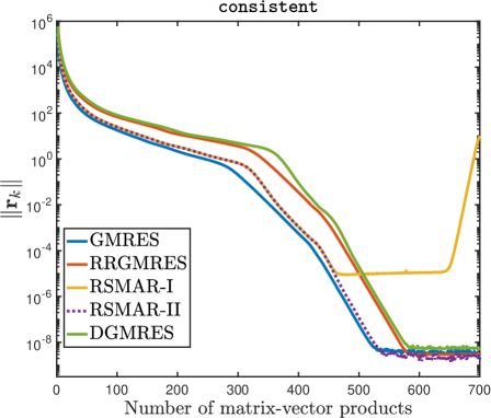
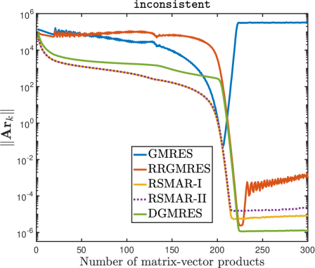
Figure 1: Residual and $\mathbf{A}$-residual histories for GMRES, RRGMRES, RSMAR, and DGMRES on singular linear systems generated from the matrix arising in the finite difference discretization of the boundary value problem (16). Left: consistent system with b = A*rand(m*m,1). Right: inconsistent system with $\mathbf{b}$ being a discretization of $f(x,y)=x+y$.

5.2 Singular symmetric linear systems

In this subsection, we compare the performance of MINRES-QLP, MINARES, and RSMAR applied to singular symmetric linear systems generated from symmetric matrices $\mathbf{A}$ from the SuitSparse Matrix Collection [8]. Three matrices (bcsstm36, zenios, and laser) are used. In each problem, we scale $\mathbf{A}$ to be $\mathbf{A}/\rho$ with $\rho=\max_{ij}|\mathbf{A}_{ij}|$, so that $\|\mathbf{A}\|\approx 1$. Consistent systems are constructed by using $\mathbf{b}=\mathbf{A}\mathbf{e}$ (with $\mathbf{e}$ a vector of ones), and inconsistent ones are done by using $\mathbf{b}=\mathbf{e}$.

We report residual histories for MINRES-QLP, MINARES, and RSMAR on consistent systems, and $\mathbf{A}$-residual histories for these algorithms on inconsistent systems. The MINARES implementation of Montoison, Orban, and Saunders [22] is referred as MINARES-II. Figures 2, 3, and 4 are on the systems generated using bcsstm36, zenios, and laser, respectively. In the consistent case for the problem bcsstm36, RSMAR-I suffers from an instability and we terminate it when the number of iterations $k=3200$. For the problem zenios, we terminate RSMAR when $k=275$ in the consistent case, and when $k=250$ in the inconsistent case. We have the following observations.

• For all problems, RSMAR-II is better than RSMAR-I and MINARES-II is better than MINARES-I in terms of the attainable optimal accuracy.

• For the problems bcsstm36 and laser, RSMAR and MINARES nearly coincide only in the initial phase, and RSMAR-II is faster than MINARES in terms of number of matrix-vector products. For the problem laser, RSMAR and MINARES nearly coincide.

• In the consistent cases for the problems bcsstm36 and laser, RSMAR-I suffers from an instability. In all consistent cases, the residual norm $\|\mathbf{r}_{k}\|$ of all algorithms is smooth before reaching the attainable optimal accuracy.

• In all inconsistent cases, the $\mathbf{A}$-residual norm $\|\mathbf{A}\mathbf{r}_{k}\|$ of RSMAR and MINARES is smooth before reaching the attainable optimal accuracy, whereas that of MINRES-QLP is erratic. MINRES-QLP suffers from an instability in the inconsistent case for the problem laser.

 

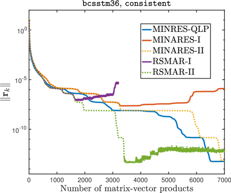
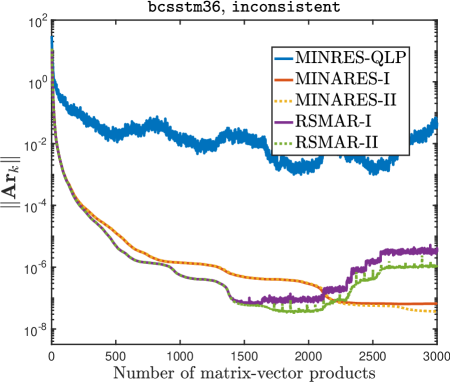
Figure 2: Residual and $\mathbf{A}$-residual histories for MINRES-QLP, MINARES, and RSMAR on singular linear systems generated from the matrix bcsstm36 ($n=23052$). Left: consistent system with $\mathbf{b}=\mathbf{A}\mathbf{e}$. Right: inconsistent system with $\mathbf{b}=\mathbf{e}$.

 

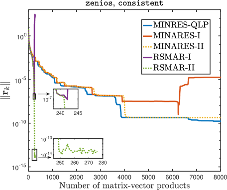
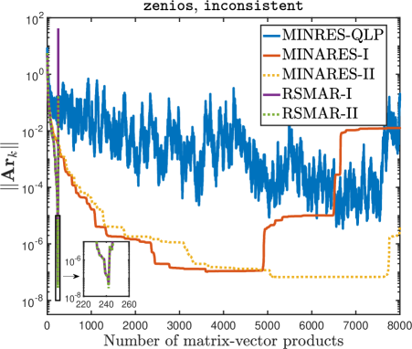
Figure 3: Residual and $\mathbf{A}$-residual histories for MINRES-QLP, MINARES, and RSMAR on singular linear systems generated from the matrix zenios ($n=2873$). Left: consistent system with $\mathbf{b}=\mathbf{A}\mathbf{e}$. Right: inconsistent system with $\mathbf{b}=\mathbf{e}$.

 

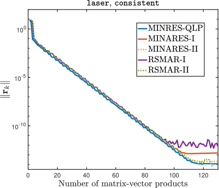
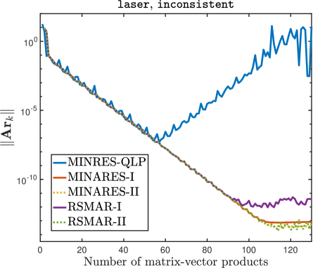
Figure 4: Residual and $\mathbf{A}$-residual histories for MINRES-QLP and MINARES on singular linear systems generated from the matrix laser ($n=3002$). Left: consistent system with $\mathbf{b}=\mathbf{A}\mathbf{e}$. Right: inconsistent system with $\mathbf{b}=\mathbf{e}$.

6 Concluding remarks and future work

RSMAR completes the family of Krylov subspace methods based on the Arnoldi process for range-symmetric linear systems. By minimizing the $\mathbf{A}$-residual norm $\|\mathbf{A}\mathbf{r}_{k}\|$ (which always converges to zero for range-symmetric $\mathbf{A}$), RSMAR can be applied to solve any range-symmetric systems. We have shown that in exact arithmetic, RSMAR and GMRES both determine the pseudoinverse solution if $\mathbf{b}\in{\rm range}(\mathbf{A})$, and terminate with the same least squares solution if $\mathbf{b}\notin{\rm range}(\mathbf{A})$. When the reached least squares solution is not the pseudoinverse solution, the lifting strategy (7) can be used to obtain it. Our numerical experiments show that on singular inconsistent range-symmetric systems, RSMAR outperforms GMRES, RRGMRES, and DGMRES, and should be the preferred method in finite precision arithmetic. As for the implementation for RSMAR, RSMAR-II is better than RSMAR-I in finite precision arithmetic.

When $\mathbf{A}$ is symmetric, RSMAR is theoretically equivalent to MINARES. The work per iteration and the storage requirements of RSMAR increase with the iterations, while MINARES remains under control even when many iterations are needed.

There are at least three possible research directions for future work. The first is about preconditioning techniques for RSMAR. The second is about stopping criteria. It would clearly be desirable to terminate the RSMAR iterations when approximately optimal accuracy has been reached. The third is the performance of RSMAR applied to linear discrete ill-posed problems. All of them are being investigated.

Our MATLAB implementations of GMRES, RRGMRES, RSMAR, DGMRES, MINRES-QLP, and MINARES are available at https://kuidu.github.io/code.html. The implementations of GMRES, RRGMRES, RSMAR, and DGMRES support restarts. All figures in section 5 can be reproduced by the MATLAB live script mar.mlx, which can be obtained from the above website.

References

• [1] W. E. Arnoldi. The principle of minimized iteration in the solution of the matrix eigenvalue problem. Quart. Appl. Math., 9:17–29, 1951.
• [2] M. Bellalij, L. Reichel, and H. Sadok. Some properties of range restricted GMRES methods. J. Comput. Appl. Math., 290:310–318, 2015.
• [3] A. Ben-Israel and T. N. E. Greville. Generalized inverses, volume 15 of CMS Books in Mathematics/Ouvrages de Mathématiques de la SMC. Springer-Verlag, New York, second edition, 2003. Theory and applications.
• [4] P. N. Brown and H. F. Walker. GMRES on (nearly) singular systems. SIAM J. Matrix Anal. Appl., 18(1):37–51, 1997.
• [5] D. Calvetti, B. Lewis, and L. Reichel. GMRES-type methods for inconsistent systems. Linear Algebra Appl., 316(1-3):157–169, 2000.
• [6] Z.-H. Cao and M. Wang. A note on Krylov subspace methods for singular systems. Linear Algebra Appl., 350:285–288, 2002.
• [7] S.-C. T. Choi, C. C. Paige, and M. A. Saunders. MINRES-QLP: A Krylov subspace method for indefinite or singular symmetric systems. SIAM J. Sci. Comput., 33(4):1810–1836, 2011.
• [8] T. A. Davis and Y. Hu. The University of Florida sparse matrix collection. ACM Trans. Math. Software, 38(1):Art. 1, 25, 2011.
• [9] K. Du, J.-J. Fan, X.-H. Sun, F. Wang, and Y.-L. Zhang. On Krylov subspace methods for skew-symmetric and shifted skew-symmetric linear systems. arXiv:2307.16460, 2023.
• [10] X. Du and D. B. Szyld. Inexact GMRES for singular linear systems. BIT, 48(3):511–531, 2008.
• [11] L. Eldén and V. Simoncini. Solving ill-posed linear systems with GMRES and a singular preconditioner. SIAM J. Matrix Anal. Appl., 33(4):1369–1394, 2012.
• [12] D. C.-L. Fong and M. Saunders. LSMR: An iterative algorithm for sparse least-squares problems. SIAM J. Sci. Comput., 33(5):2950–2971, 2011.
• [13] A. Greenbaum, F. Kyanfar, and A. Salemi. On the convergence rate of DGMRES. Linear Algebra Appl., 552:219–238, 2018.
• [14] C. Greif, C. C. Paige, D. Titley-Peloquin, and J. M. Varah. Numerical equivalences among Krylov subspace algorithms for skew-symmetric matrices. SIAM J. Matrix Anal. Appl., 37(3):1071–1087, 2016.
• [15] K. Hayami and M. Sugihara. A geometric view of Krylov subspace methods on singular systems. Numer. Linear Algebra Appl., 18(3):449–469, 2011.
• [16] K. Hayami, J.-F. Yin, and T. Ito. GMRES methods for least squares problems. SIAM J. Matrix Anal. Appl., 31(5):2400–2430, 2010.
• [17] L.-Y. Hong and N.-M. Zhang. On the preconditioned MINRES method for solving singular linear systems. Comput. Appl. Math., 41(7):Paper No. 304, 21, 2022.
• [18] I. C. F. Ipsen and C. D. Meyer. The idea behind Krylov methods. Amer. Math. Monthly, 105(10):889–899, 1998.
• [19] C. Lanczos. An iteration method for the solution of the eigenvalue problem of linear differential and integral operators. J. Research Nat. Bur. Standards, 45:255–282, 1950.
• [20] Y. Liu, A. Milzarek, and F. Roosta. Obtaining pseudo-inverse solutions with MINRES. arXiv:2309.17096, 2023.
• [21] C. D. Meyer. Matrix analysis and applied linear algebra. Society for Industrial and Applied Mathematics (SIAM), Philadelphia, PA, 2023. Second edition.
• [22] A. Montoison, D. Orban, and M. A. Saunders. MINARES: An iterative solver for symmetric linear systems. arXiv:2310.01757, 2023.
• [23] K. Morikuni and K. Hayami. Inner-iteration Krylov subspace methods for least squares problems. SIAM J. Matrix Anal. Appl., 34(1):1–22, 2013.
• [24] K. Morikuni and K. Hayami. Convergence of inner-iteration GMRES methods for rank-deficient least squares problems. SIAM J. Matrix Anal. Appl., 36(1):225–250, 2015.
• [25] K. Morikuni and M. Rozložník. On GMRES for singular EP and GP systems. SIAM J. Matrix Anal. Appl., 39(2):1033–1048, 2018.
• [26] A. Neuman, L. Reichel, and H. Sadok. Algorithms for range restricted iterative methods for linear discrete ill-posed problems. Numer. Algorithms, 59(2):325–331, 2012.
• [27] A. Neuman, L. Reichel, and H. Sadok. Implementations of range restricted iterative methods for linear discrete ill-posed problems. Linear Algebra Appl., 436(10):3974–3990, 2012.
• [28] C. C. Paige and M. A. Saunders. Solutions of sparse indefinite systems of linear equations. SIAM J. Numer. Anal., 12(4):617–629, 1975.
• [29] L. Reichel and Q. Ye. Breakdown-free GMRES for singular systems. SIAM J. Matrix Anal. Appl., 26(4):1001–1021, 2005.
• [30] Y. Saad and M. H. Schultz. GMRES: A generalized minimal residual algorithm for solving nonsymmetric linear systems. SIAM J. Sci. Statist. Comput., 7(3):856–869, 1986.
• [31] A. Sidi. A unified approach to Krylov subspace methods for the Drazin-inverse solution of singular nonsymmetric linear systems. Linear Algebra Appl., 298(1-3):99–113, 1999.
• [32] A. Sidi. DGMRES: A GMRES-type algorithm for Drazin-inverse solution of singular nonsymmetric linear systems. Linear Algebra Appl., 335:189–204, 2001.
• [33] L. Smoch. Some results about GMRES in the singular case. Numer. Algorithms, 22(2):193–212, 1999.
• [34] L. Smoch. Spectral behaviour of GMRES applied to singular systems. Adv. Comput. Math., 27(2):151–166, 2007.
• [35] K. Sugihara, K. Hayami, and L. Zeyu. GMRES using pseudoinverse for range symmetric singular systems. J. Comput. Appl. Math., 422:Paper No. 114865, 15, 2023.
• [36] K. Sugihara, K. Hayami, and N. Zheng. Right preconditioned MINRES for singular systems. Numer. Linear Algebra Appl., 27(3):e2277, 25, 2020.
• [37] H. F. Walker and L. Zhou. A simpler GMRES. Numer. Linear Algebra Appl., 1(6):571–581, 1994.
• [38] G. Wang, Y. Wei, and S. Qiao. Generalized inverses: theory and computations, volume 53 of Developments in Mathematics. Springer, Singapore; Science Press Beijing, Beijing, second edition, 2018.
• [39] Y. Wei and H. Wu. Convergence properties of Krylov subspace methods for singular linear systems with arbitrary index. J. Comput. Appl. Math., 114(2):305–318, 2000.
• [40] N. Zhang. A note on preconditioned GMRES for solving singular linear systems. BIT, 50(1):207–220, 2010.
• [41] J. Zhou and Y. Wei. Stagnation analysis of DGMRES. Appl. Math. Comput., 151(1):27–39, 2004.
• [42] J. Zhou and Y. Wei. The analysis of restart DGMRES for solving singular linear systems. Appl. Math. Comput., 176(1):293–301, 2006.
• [43] J. Zhou and Y. Wei. A simpler DGMRES. Appl. Math. Comput., 217(1):124–129, 2010.