An effective geometric distortion solution and its implementation

Abstract

Context. Geometric distortion (GD) critically constrains the precision of astrometry. Its correction required GD calibration observations, which can only be obtained using a special dithering strategy during the observation period. Some telescopes lack GD calibration observations, making it impossible to accurately determine the GD effect using well-established methods. This limits the value of the telescope observations in certain astrometric scenarios, such as using historical observations of moving targets in the solar system to improve their orbit.

Aims. We investigated a method for handling GD that does not rely on the calibration observations. With this advantage, it can be used to solve the GD models of telescopes which were intractable in the past. Consequently, astrometric results of the historical observations obtained from these telescopes can be significantly improved.

Methods. We used the weighted average of the plate constants to derive the GD model. The method was implemented in Python and released on GitHub. It was then applied to solve GD in the observations taken with the 1-m and 2.4-m telescopes at Yunnan Observatory. The resulting GD models were compared with those obtained using well-established methods to demonstrate the accuracy. Furthermore, the method was applied in the reduction of observations for two targets, the moon of Jupiter (Himalia) and the binary GSC2038-0293, to show its effectiveness.

Results. The GD of the 60-cm telescope at Yunnan Observatory without calibration observations was accurately solved by our method. After GD correction, the astrometric results for both targets show improvements. Notably, the mean residual between observed and computed position ($O-C$) for the binary GSC2038-0293 decreased from 36 mas to 5 mas.

1 Introduction

Both space and ground-based observations in the field of optical astrometry are inevitably affected by geometric distortion (GD). Various factors contribute to GD, such as flaws in the shape of optical components, installation deviations, irregularities in filters, and manufacturing imperfections in CCD detectors (Bernard et al., 2018).

In the majority of scenarios, GD serves as the main effect limiting high-precision astrometry (Peng et al., 2017; Wang et al., 2017; McKay & Kozhurina-Platais, 2018; Wang et al., 2019; Casetti-Dinescu et al., 2021). For example, observations captured by the UVIS channel of the Wide Field Camera 3 on the Hubble Space Telescope (HST) would be affected by GD, causing shifts of up to 35 pixels (McKay & Kozhurina-Platais, 2018); For the observations taken with the 2.4-m telescope at Yunnan Observatory, the astrometric precision nearly improved by a factor of 2 after GD correction (Peng et al., 2017).

Besides its effect on astrometric precision, GD correction is also necessary for some applications to improve computational speed or meet fundamental requirements. For instance, in real-time applications that involve handling substantial data and computational loads for detecting and tracking near-Earth objects, Zhai et al. (2018) employed GD correction when converting the pixel coordinate to the equatorial coordinate, so that this process was accelerated while achieving high-precision results (Zheng et al., 2021).

Adopting high-order plate constants for reduction can mitigate the effect of GD. However, it requires sufficient reference stars exist in the field of view (FOV), which is not met in specific high-precision applications. For some ground-based observations of moving targets, instrument limitations and other factors may result in a lack of observed reference stars available from the observations. Consequently, the GD solution derived from calibration observations is essential for obtaining high-precision positions of these moving targets. In addition, in HST extremely deep field observations where the AB magnitude of stars can reach up to 30 mag (Illingworth et al., 2013), there is no star catalogue that provides accurate positions for reference stars. The infeasibility of applying the high-order plate constants, as a result, makes GD correction necessary.

The most notable research on addressing GD is the study conducted by Anderson & King (2003), which focuses on the GD effect of the Wide Field Planetary Camera 2 (WFPC2) installed on the HST. The GD effect at the edges of the WFPC2 FOV reached up to 5 pixels, severely degrading the astrometric precision of the HST. For this reason, Anderson & King (2003) developed a self-calibration technique using observations acquired at various orientations. After GD correction, the average positional residuals decreased to 0.02 pixels and 0.01 pixels for the planetary camera and the wide-field camera, respectively. From then on, the HST started to fully demonstrate its astrometric potential. This self-calibration technique, which does not rely on a star catalogue, has been applied to solve GD for multiple cameras on the HST (Bellini & Bedin, 2009) as well as several ground-based telescopes (Anderson et al., 2006; Bellini & Bedin, 2010), achieving high-precision astrometry.

An alternative approach for solving GD is based on the known reference star positions that are not affected by GD. These positions can be calculated by an external astrometric reference system, such as a high-precision astrometric catalogue, HST observation positions with GD correction (Service et al., 2016), or even star positions obtained from non-optical wavelength bands (Reid & Menten, 2007). By comparing the positional deviations between observed and reference positions, the influence of GD on astrometry can be determined. This method requires fewer observations for GD solution than the self-calibration technique, but the accuracy may be affected by the errors present in the external reference system (Bernard et al., 2018). Peng et al. (2012) proposed a novel method for mitigating the influence of catalogue errors on GD solution. This method involves algebraically manipulating the measurement errors of identical stars across different frames, thereby reducing the accuracy requirements of the external reference catalogue. Furthermore, it has been improved by Wang et al. (2019) to handle the GD in observations captured by the 2.3-m Bok telescope at Kitt Peak (Peng et al., 2023).

The above methods can effectively solve the GD model and achieve positional measurements with precision up to the 0.01 pixel level. Nonetheless, these methods necessitate well-planned observational strategies, obtaining optimally dithered and overlapping frames (Anderson & King, 2003; Peng et al., 2012), to offset the effects of GD or catalogue errors (Zheng et al., 2021). These GD calibration observations require additional telescope time. It is sometimes difficult to meet due to observation conditions. More importantly, some telescopes may not have had such observation plans for a significant period of time. Due to the dynamic changes in GD, a prolonged absence of GD calibration observations can substantially degrade the accuracy of the astrometry.

To address this issue, a method is proposed to derive an analytical GD model without the requirement of GD calibration observations. We demonstrate the performance of this method by comparing it with the well-established GD correction method (Peng et al., 2012; Wang et al., 2019). Additionally, we perform the reduction of Himalia (J6) observations captured by the 2.4-m telescope at Yunnan Observatory and the 60-cm telescope observations for a low-mass close binary system GSC02038-00293 (Dal et al., 2012). These observations are initially reduced using plate constants without GD correction, but the results are unsatisfactory. Like many telescopes primarily employed for photometric purposes, the 60-cm telescope at Yunnan Observatory has never performed any GD calibration observations. However, a novel research focus of the binary GSC02038-00293 highlights the importance of astrometry. Since our method is effective and easy to implement, it is especially applicable at this time. Applying our method to correct GD significantly improves the astrometry of the targets, leading to more reliable results than any other reduction methods. The results indicate that our method is particularly useful for reducing historical observations that lack of GD calibration observations. The advantages of our method make it valuable in studying the long-term changes in the positions of the targets, as well as their formation and evolution. A Python implementation of this method is available on GitHub.

This paper is structured as follows: Section 2 provides detailed information about the observations and the corresponding instruments used to capture them, while Section 3 describes the GD correction method based on the Gaia DR3 (Gaia Collaboration et al., 2023). Section 4 presents the performance comparison between our method and the well-established method, as well as the advantages of the new method in reducing the observations of the targets J6 and GSC02038-00293. Finally, Section 5 concludes the paper with some closing remarks.

2 Observations

Observations obtained from multiple telescopes are used in this paper. These telescopes include the 60-cm telescope (Zang et al., 2022), the 1-m telescope (IAU code 286, longitude–E$102^{\circ}47^{\prime}18^{\prime\prime}$, latitude–N$25^{\circ}1^{\prime}46^{\prime\prime}$, and height–2000m above sea level) at Yunnan Observatory, and the 2.4-m telescope (IAU code O44, longitude–E$100^{\circ}1^{\prime}51^{\prime\prime}$, latitude–N$26^{\circ}42^{\prime}32^{\prime\prime}$, and height–3193m above sea level) at Yunnan Observatory (YNO 60-cm, YNO 1-m, and YNO 2.4-m). More instrumental details of the reflectors and CCD detectors are listed in Table 1. The patterns and magnitudes of GD experienced by these instruments are different.

Observation sets 1 and 2 were captured using the dithering strategy, which takes multiple dithered exposures of the same sky field with different offsets (Peng et al., 2012). They are used to demonstrate that the proposed method in this paper achieves the same accuracy as other well-established GD correction methods. Observation sets 3 and 4 are significantly affected by higher-order GD, but only a dozen or so bright stars can be used to solve the plate constants, thus the GD solution is very important for high-precision astrometry of the targets. The detailed information of these observations is provided in Table 2. In this paper, bright stars refer to the stars with sufficient signal-to-noise ratio, whose astrometric precision is not dominated by centering errors.

Table 1: Specifications of the 1-m and 2.4-m telescopes and the corresponding CCD detectors.

Parameter	1-m telescope	2.4-m telescope	60-cm telescope
Approximate focal length	1330 cm	1920 cm	750 cm
F-Ratio	13.1	8.0	12.5
Diameter of primary mirror	101.6 cm	240.0 cm	60.0 cm
Approximate scale factor	0.234 arcsec pixel-1	0.283 arcsec pixel-1	0.383 arcsec pixel-1
Size of CCD array (effective)	4096 $\times$ 4112	1900 $\times$ 1900	2048 $\times$ 2048
Size of pixel	15.0 $\mu m\ \times$ 15.0 $\mu m$	13.5 $\mu m\ \times$ 13.5 $\mu m$	13.5 $\mu m\ \times$ 13.5 $\mu m$

Table 2: Details of the observations. The first column is the identification of the observation set. Column (2) and Column (3) list the target and the observational date. Column (4) gives the number of CCD frames in each observation set. Column (5) is the range of zenith distance. Column (6) is the telescope used. Column (7) provides the number of stars with sufficient signal-to-noise ratio, whose astrometric precision is not dominated by centering errors. Column (8) gives the exposure time.

ID	Target	Obs Date	Frames	Zenith Distance	Telescope	Bright Star	Exposure
		(y-m-d)	(No.)	(degree)		(No.)	(second)
(1)	(2)	(3)	(4)	(5)	(6)	(7)	(8)
1	NGC2168	2018-11-13	38	1$\sim$17	YNO 1-m	350$\sim$400	60
2	NGC1664	2015-02-10	44	19$\sim$21	YNO 2.4-m	150$\sim$180	40
3	Himalia	2017-04-08	15	35$\sim$37	YNO 2.4-m	$\sim$10	30
4	GSC02038-00293	2011-02-28	187	1$\sim$30	YNO 60-cm	$\sim$12	40

3 Methods

The method investigated in this paper derives an analytical GD model, which is characterized by a high-order polynomial, using the distortionless positions of stars provided by the Gaia catalogue. The analytical GD model can effectively describe the GD effect in ground-based observations, because the majority of GD components can be characterized by polynomials. The remaining components, which are typically described using a lookup table (Wang et al., 2019), generally only account for a minor portion of GD. This is confirmed in the subsequent section through experimentation.

This method extracts the GD effect present in each frame of observations, and then derives the GD model based on the GD effect extracted from these multiple frames. The implementation details of this method are as follows. A two-dimensional Gaussian fitting is used to determine the pixel positions of the observed stars. These observed stars are then cross-matched with the stars given in the Gaia catalogue (Gaia Collaboration et al., 2023) to obtain their reference positions. Specifically, the reference positions are topocentric astrometric positions of the stars calculated from their catalogue positions. To ensure the accuracy of the GD solution, we also account for additional factors that may cause deterioration to its accuracy. These factors include differential colour refraction and charge transfer efficiency issues, which can be effectively addressed using the method presented in Lin et al. (2020). Consequently, we can obtain the pixel coordinate $(x_{i},y_{i})$ and the equatorial coordinate $(\alpha_{i},\delta_{i})$ of each star $i$. The standard coordinate $(\xi_{i},\eta_{i})$ can be converted from the equatorial coordinate via the central projection, which is presented in Green (1985).

To extract the GD effect on pixel positions, we need to solve a six-parameter linear transformation to obtain the approximate pixel positions $(x_{i}^{{}_{L}},y_{i}^{{}_{L}})$ of the reference stars. The linear transformation is expressed as:

$$\begin{gathered}x_{i}=\widetilde{a}\xi_{i}+\widetilde{b}\eta_{i}+\widetilde{c},\\ y_{i}=\widetilde{d}\xi_{i}+\widetilde{e}\eta_{i}+\widetilde{f},\end{gathered}$$ (1)

where the coefficients $\widetilde{a}$$\sim$$\widetilde{f}$ (denoted as $C^{{}_{L}}_{\text{std}}$ hereafter) can be estimated through the least-squares fitting. Using the linear transformation, the standard coordinates $(\xi_{i},\eta_{i})$ can be converted to the approximate pixel positions $(x_{i}^{{}_{L}},y_{i}^{{}_{L}})$. The coefficients of the linear transformation $C^{{}_{L}}_{\text{std}}$ are initially inaccurate because they are affected by the GD. During the iterative solving process of GD, the pixel positions $(x_{i},y_{i})$ in Equation 1 will be replaced by the positions after GD correction in each new iteration. As a result, the approximate pixel positions $(x_{i}^{{}_{L}},y_{i}^{{}_{L}})$ would converge to the distortionless pixel positions.

Based on the pattern and magnitude of GD experienced by the optical system of each telescope, we select a polynomial of appropriate order $N$ to characterize its analytical GD model. The general formula of the polynomial is given as:

$$\begin{gathered}U=\sum_{m,n,0\leqslant m+n\leqslant N}k_{mn}X^{m}Y^{n},\\ V=\sum_{m,n,0\leqslant m+n\leqslant N}j_{mn}X^{m}Y^{n},\end{gathered}$$ (2)

where $k_{mn}$ and $j_{mn}$ are the parameters to be fitted. Setting $(X,Y)$ as coordinates $(x_{i}^{{}_{L}},y_{i}^{{}_{L}})$ and $(U,V)$ as coordinates $(x_{i},y_{i})$, an $N$th-order polynomial that characterizes the GD effect can be fitted. We denote the coefficients of this polynomial as $C_{\text{pix}}$. By solving for the coefficients $C_{\text{pix}}$ of each frame in an observation set and applying a weighted average based on image quality, an average GD solution $\overline{C}_{\text{pix}}$ can be obtained. Most of the random errors are offset in the weighted average of the information from multiple frames, leaving only the GD effect.

Now we can determine the GD effect at any given pixel position using a polynomial with coefficients $\overline{C}_{\text{pix}}$. However, when the GD effect changes dramatically within a small image range, there would be a significant difference in the GD effect between the distortionless pixel position of the star and its actual observed pixel position. In order to handle this issue, we determine the transformation from the pixel positions $(x_{i},y_{i})$ to the distortionless positions to correct GD. Specifically, we construct a $16\times 16$ grid uniformly distributed across the pixel coordinates of the image (as shown in Figure 2). Then the grid positions $(x_{g},y_{g})$ are transformed via a polynomial using the coefficients $\overline{C}_{\text{pix}}$, resulting in their distorted positions $(x_{g}^{{}_{GD}},y_{g}^{{}_{GD}})$. Finally, the inverse transformation coefficients $\overline{C}_{\text{inv}}$ are determined by fitting from $(x_{g}^{{}_{GD}},y_{g}^{{}_{GD}})$ to $(x_{g},y_{g})$. The pixel position with GD correction can be calculated by setting $(X,Y)$ as the coordinate $(x_{i},y_{i})$ and using $\overline{C}_{\text{inv}}$ as the coefficients in Equation 2. Figure 1 describes the solving process for these coefficients and the transformations between different positions.

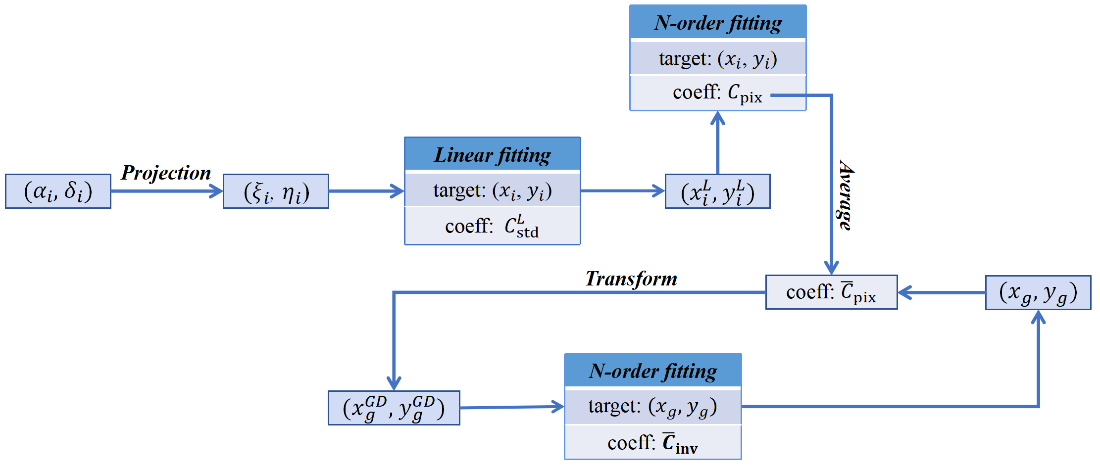
Figure 1: The transformations between different positions and the solving process of the corresponding coefficients in one iteration of our geometric distortion (GD) solution. The arrows in the figure indicate the processes of coordinate transformations through the given coefficients, as well as other operational processes denoted in bold. The target in the figure represents the fitting targets of the input positions, while the coeff denotes the fitted coefficients obtained from the fitting process.

Considering that the pixel positions of stars are contaminated by different levels of random noise, weights have been introduced into all fitting procedures related to the pixel positions $(x_{i},y_{i})$. The GD model is derived through an iterative procedure, with the weights initially set to be uniform. After the first iteration of the GD solution, the weight for each star is determined as the inverse of the variance in positional measurements. The variance can be calculated by fitting a sigmoidal function to the Mag-SD data (as shown in Figure 3). The sigmoidal function is expressed as:

$$\sigma(m)=(A_{1}-A_{2})/(1+e^{(m-m_{0})/dm})+A_{2},$$ (3)

where $m$ is the magnitude of the star, $\sigma(m)$ is the positional SD of the star in the previous iteration, $A_{1},A_{2},m_{0}$ and $dm$ are the free parameters. Detailed calculation procedure for the weights can be found in Lin et al. (2019). The weights and the coefficients $C^{{}_{L}}_{\text{std}}$ are updated in each iteration, so that a more accurate GD model can be solved. The final analytical GD model is obtained through two to four iterations of the aforementioned procedure.

For comparison, a classical method of the plate constants reduction is also applied in this paper. The method can be simply described as solving a polynomial transformation from pixel positions of reference stars to their standard positions, and then using the transformation to calculate the astrometric position of the target. Using a $N$th-order polynomial for reduction, GD not higher than $N$th-order can be handled if there are enough reference stars (Green, 1985; Peng & Fan, 2010).

4 Results

Compared with the GD model determined by the well-established method (Peng et al., 2012; Wang et al., 2019), the accuracy of the GD model obtained through our method is verified. Furthermore, our method is applied to reduce observations of Himalia (J6) and GSC02038-00293 to demonstrate its advantages.

4.1 Comparison with the well-established method

Since observation sets 1 and 2 were acquired by the dithering strategy, the well-established methods can also be used to solve GD. The GD models for these observation sets were solved by the methods described in Wang et al. (2019) and Section 3, respectively. Figure 2 presents the results, which include the GD models for the YNO 1-m and 2.4-m telescopes solved by each method. The differences of the GD models solved by these two methods for each telescope are also presented in the right panels of the figure. The analytical GD model for the YNO 1-m telescope is characterized using a 4th-order polynomial, while the model for the YNO 2.4-m telescope using a 5th-order polynomial.

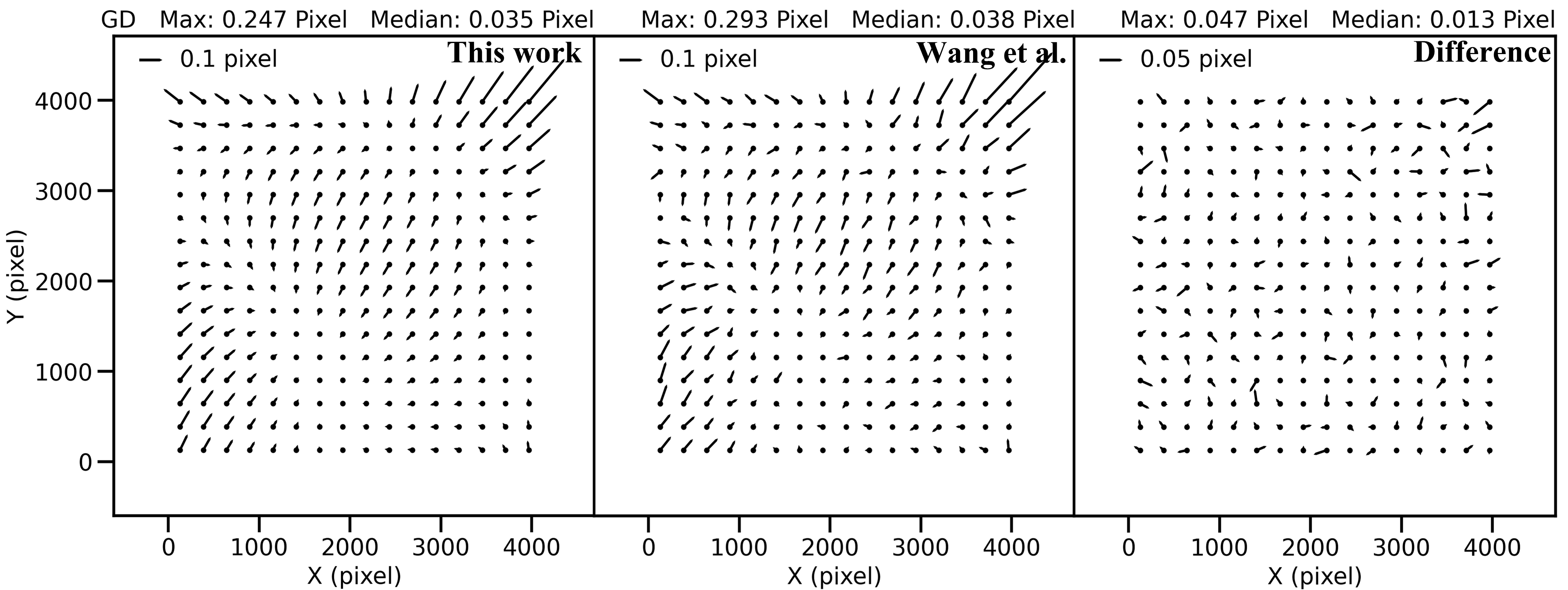
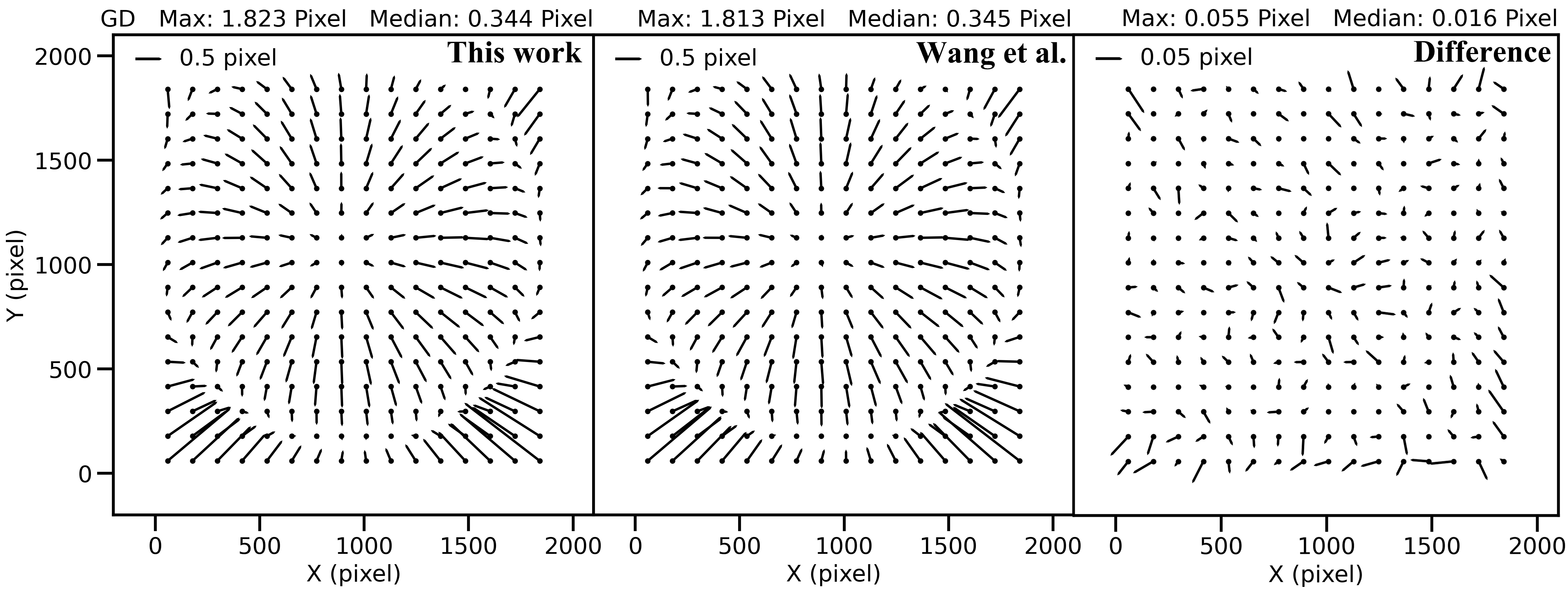
Figure 2: The GD models of the YNO 1-m and 2.4-m telescopes solved by our method and the method of Wang et al. (2019), respectively. The differences of these two GD solutions for each telescope are presented in the right panels. The upper panels display the GD models of the YNO 1-m telescope, while the lower panels show the GD models of the YNO 2.4-m telescope. The statistics of the GD vectors are presented at the top of each panel. The vectors are suitably magnified to clearly visualize the shape of the GD.

After GD correction, the six-parameter plate constants are used for the reduction of observations to obtain astrometric results. Hereafter, the astrometric results corrected by the method of Wang et al. (2019) are used as a reference. Figure 3 shows the positional standard deviation (SD) of each star, which is calculated as $\sigma_{\text{sum}}=\scriptstyle{\sqrt{\sigma_{\alpha\cos\delta}^{2}+\sigma_{\delta}^{2}}}$. In addition, the difference in the mean $(O-C)$ (i.e., the residual between the observed and computed position) between our results and the reference results is shown in Figure 4. As can be seen from Figure 3 and 4, the astrometric results corrected using our GD solution are consistent with the reference results. For the YNO 1-m telescope observations, which is less affected by GD, the mean $(O-C)$ difference between our results and the reference results is merely 1 mas. The difference is only 2 mas for the observations captured by the YNO 2.4-m telescope. In addition, the SDs of the astrometric results obtained by the two methods are equivalent. That is to say, the method proposed in this paper can efficiently correct GD and obtain reliable astrometric results.

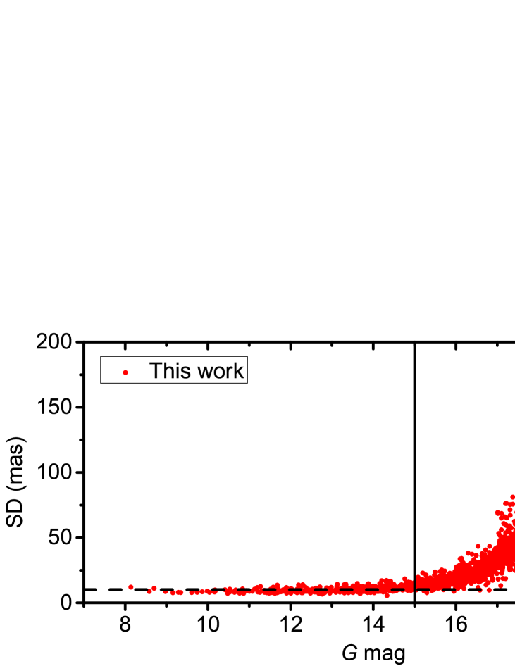
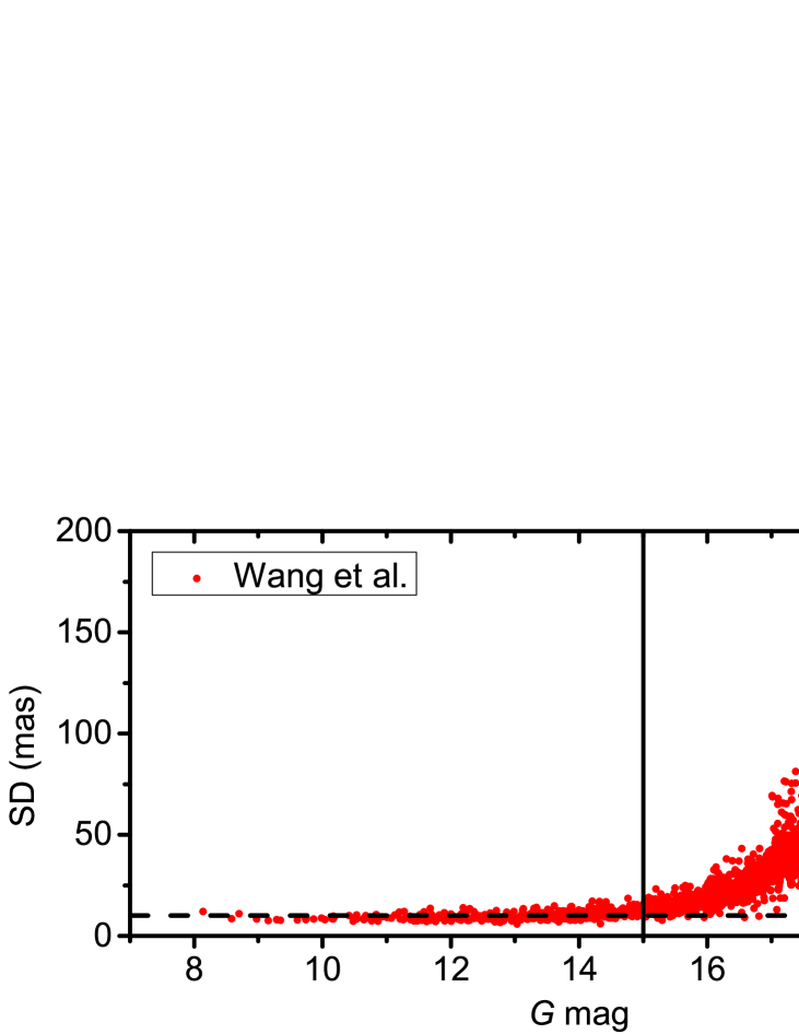
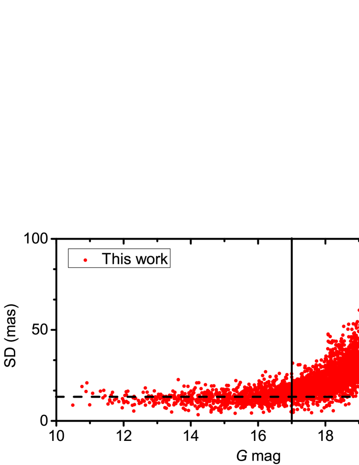
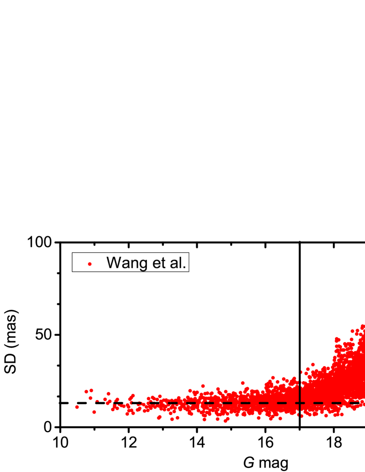
Figure 3: Comparison of the positional standard deviation (SD) obtained after GD correction using our method versus the reference method (Wang et al., 2019). The upper panels present the results for observation set 1 captured by the YNO 1-m telescope, and the bottom panels show the results for observation set 2 captured by the YNO 2.4-m telescope. The horizontal axis is Gaia G-mag and the vertical axis is the positional SD calculated by $\sigma_{\text{sum}}=\scriptstyle{\sqrt{\sigma_{\alpha\cos\delta}^{2}+\sigma_{\delta}^{2}}}$. The horizontal dashed line marks the median of the positional SDs for stars brighter than the magnitude indicated by the vertical line, the number on the right is the median.

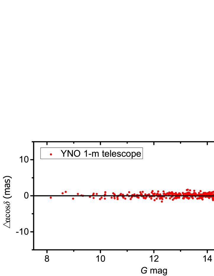
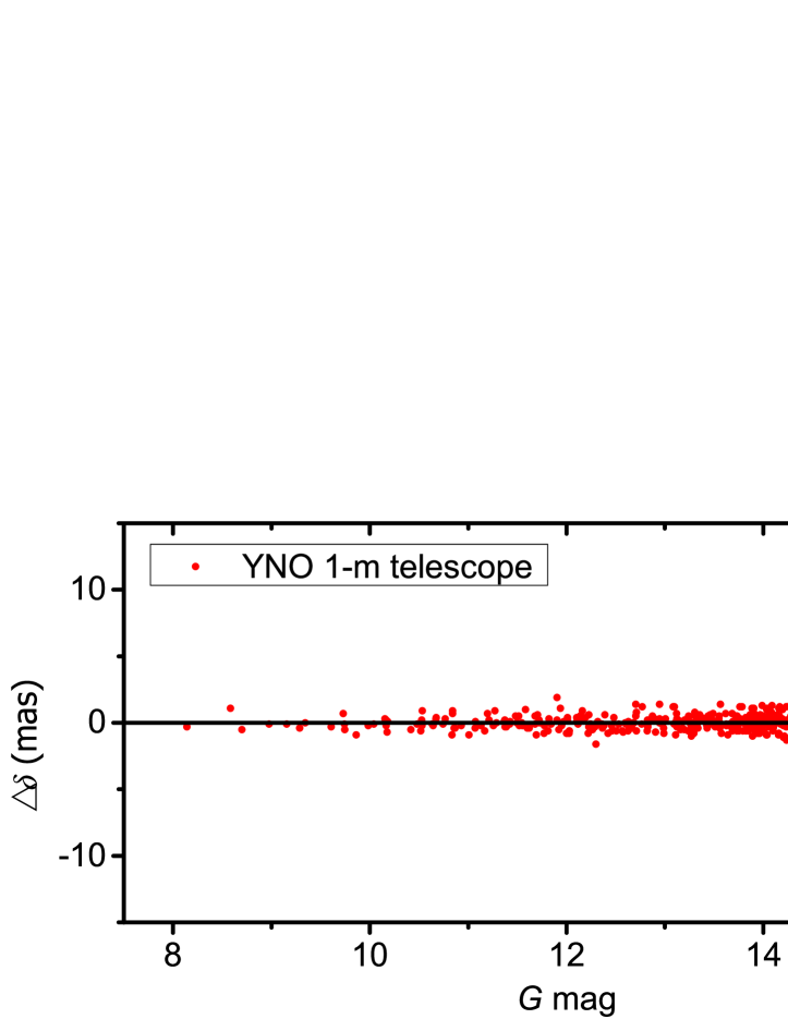
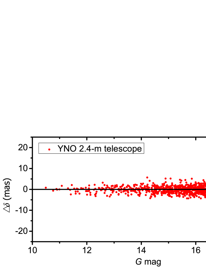
Figure 4: The differences of the mean $(O-C)$ in R.A. and Decl directions between our results and the reference results. The upper panels are the results for observation set 1 and the bottom panels are for observation set 2. Stars with low signal-to-noise ratios are excluded. The standard deviation of these differences $\sigma$ is shown in each panel.

4.2 Application of the GD solution

As stated in Section 1, our method is particularly useful in scenarios where only a limited number of bright reference stars (typically a dozen or so) can be used in the reduction. This usually happens when observing a sparse FOV, where the moving target may pass through. In this section, we processed and analyzed the observations of two targets that satisfy the scenario. These observations were not taken with a dithered FOV. Hence, the aforementioned well-established GD solutions are not applicable.

Figure 5 shows the astrometric results of the J6 observations captured by the YNO 2.4-m telescope, the upper panel shows an obviously greater SD for the target than other bright stars. This is because there are insufficient reference stars available for reduction, leading to overfitting of the 3rd-order plate constants.

To address this issue, we corrected the GD corresponding to the 3rd-order polynomial using the method proposed in this work, and then used the six-parameter plate constants for reduction. The astrometric precision of the target J6 is improved after GD correction, with the positional SD decreased from 20 mas to 17 mas. The result is shown in the lower panel of Figure 5.

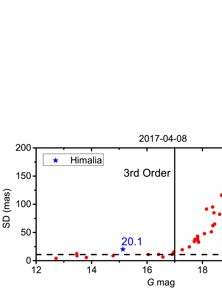
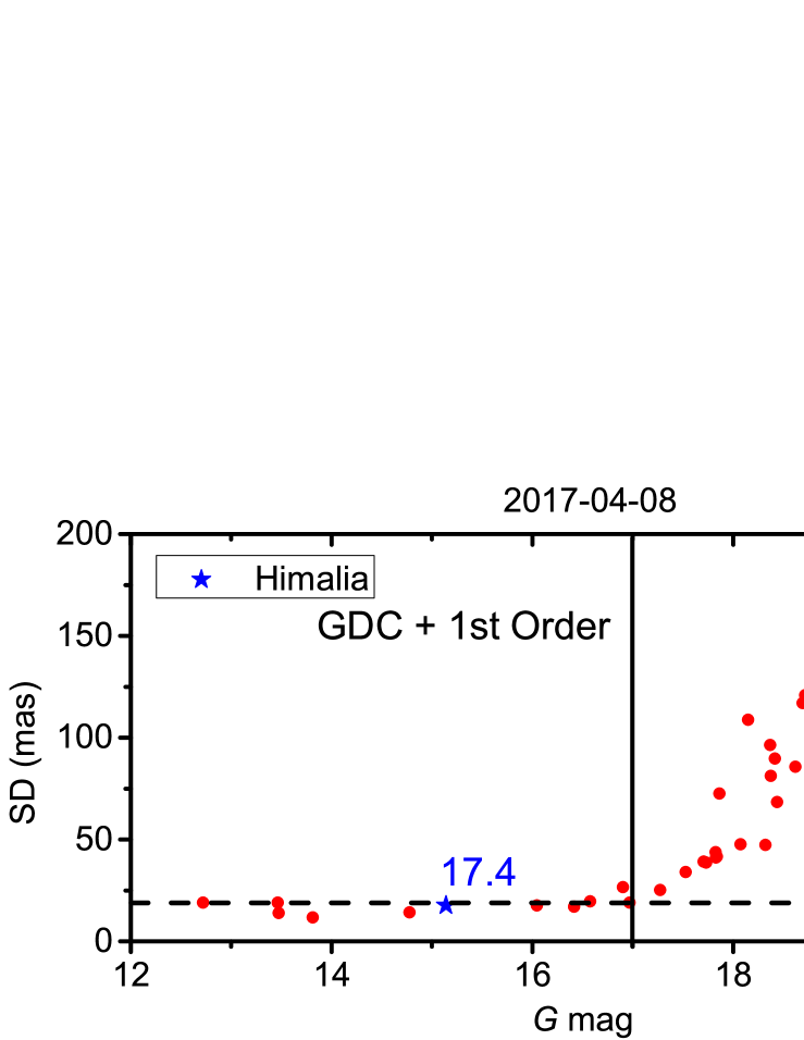
Figure 5: The positional SD of Himalia (J6) before and after the GD correction.

The improvement is more significant for the observations taken with the YNO 60-cm telescope. Figure 6 shows the GD model of the telescope solved with observation set 4. To obtain reliable astrometric results, this GD solution was applied in the reduction of observation set 4. For comparison, Figure 7 also presents the results obtained by using plate constants of different order for reduction. The left panel in the figure gives the positional SD and the right panel the corresponding mean $(O-C)$ calculated by $\langle O-C\rangle_{\mathrm{sum}}=\scriptstyle{\sqrt{\langle O-C\rangle_{\alpha\cos\delta}^{2}+\langle O-C\rangle_{\delta}^{2}}}$.

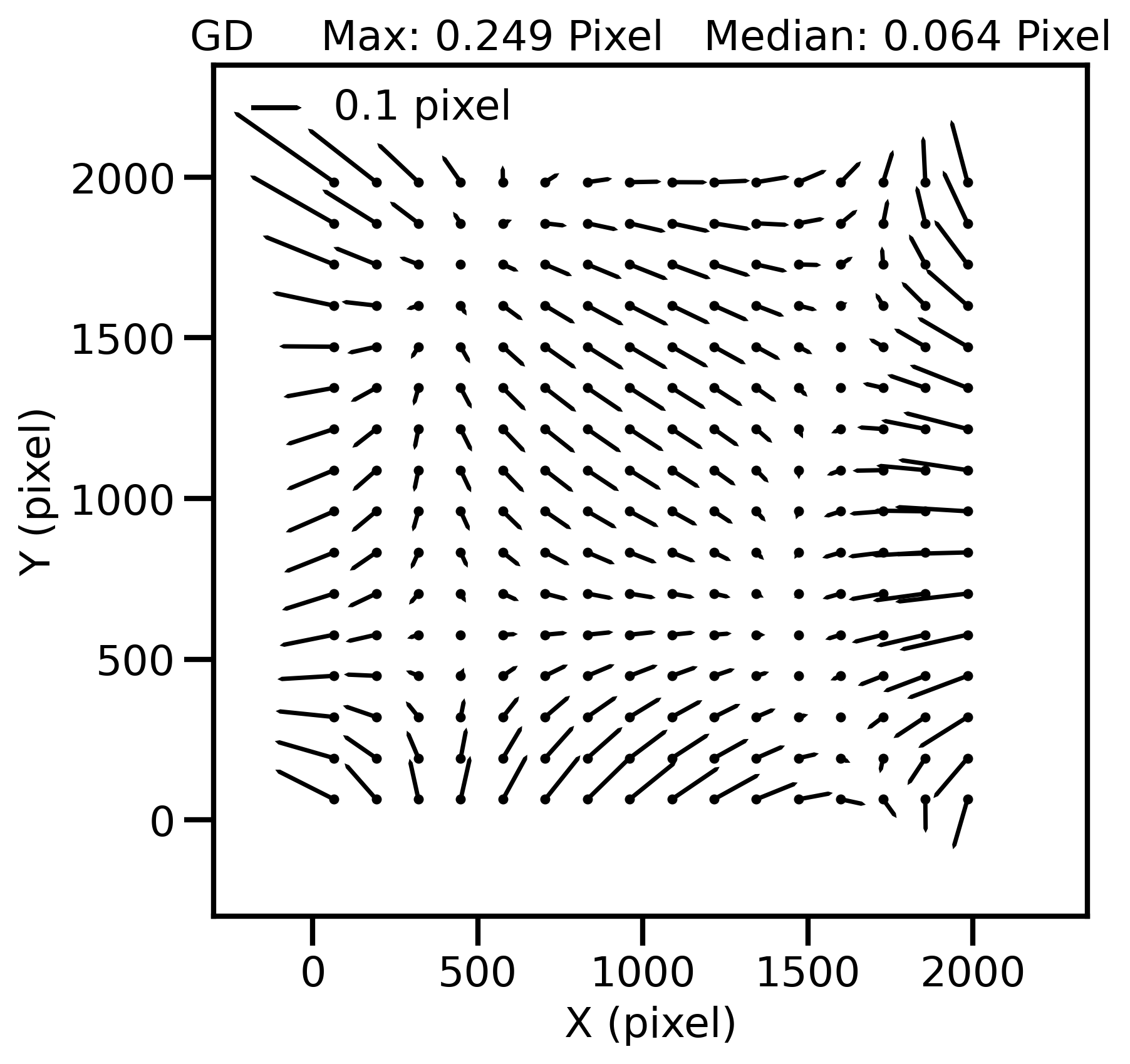
Figure 6: The GD model of YNO 60-cm telescope.

Due to the observation set points to a fixed FOV, using low-order plate constants for reduction is possible to achieve precise positional measurement for the target (see 25.0 mas in panel (a) of Figure 7). However, despite the good fit of the plate constants at this time, the results for all stars displayed in the right panel (b) show large mean $(O-C)$, suggesting the presence of significant GD effect and rendering these astrometric results unreliable. As the order of the plate constants increased, the positional SD of the target given in panels (c) and (e) becomes greater than that of other bright stars. That is to say, even if only 2nd-order plate constants are used, overfitting will occur and become more pronounced as the order increases. This is consistent with the previous astrometric results of J6 observations. Additionally, panels (d) and (f) show that the mean $(O-C)$ values of the reference stars are decreased. This is due to overfitting resulting in the residual being absorbed in the reduction process. The target should not be involved in the fitting of the plate constants, so its mean $(O-C)$ values remain large, indicating unsatisfactory astrometric results.

The bottom two panels in Figure 7 provide the results of applying our GD correction method first, followed by reduction using the six-parameter plate constants. As evident from the panels, these results show significant advantages compared to the results of other methods. On the one hand, the astrometric precision of the target is comparable to that achieved using the low-order plate constants. On the other hand, panel (h) reveals that the mean $(O-C)$ values for both the target and the reference stars are significantly smaller than those obtained using the 2nd and 3rd-order plate constants. This demonstrates that the system error caused by GD is significantly decreased after applying the GD correction.

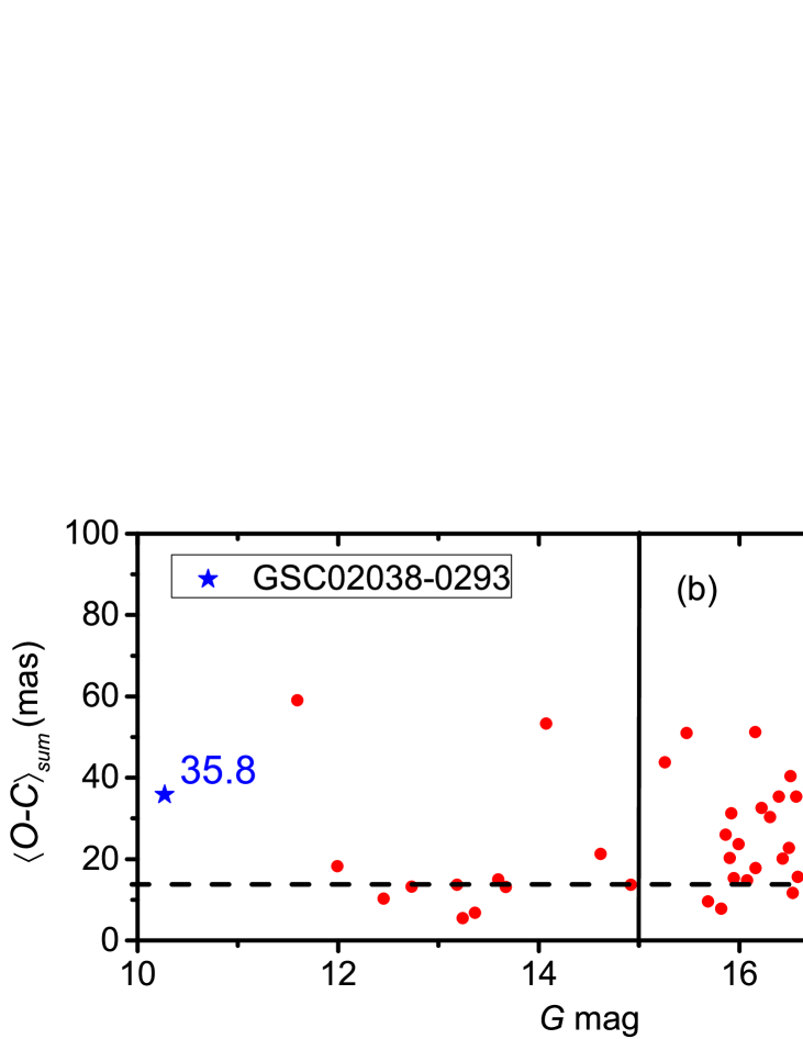
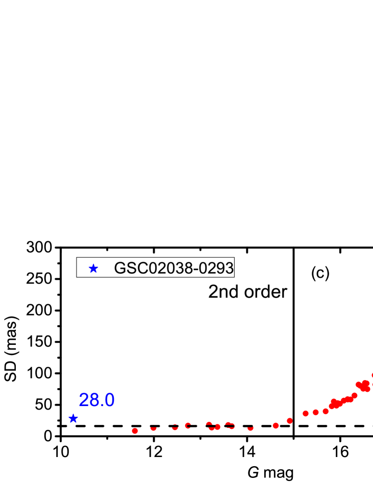
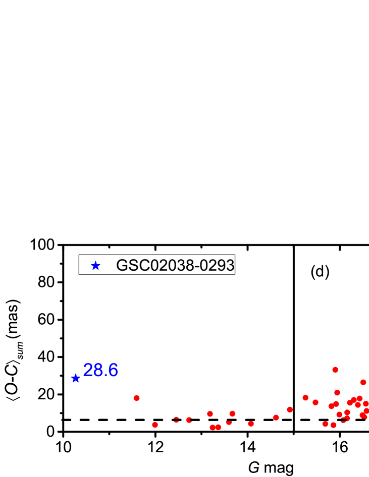
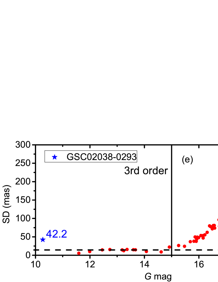
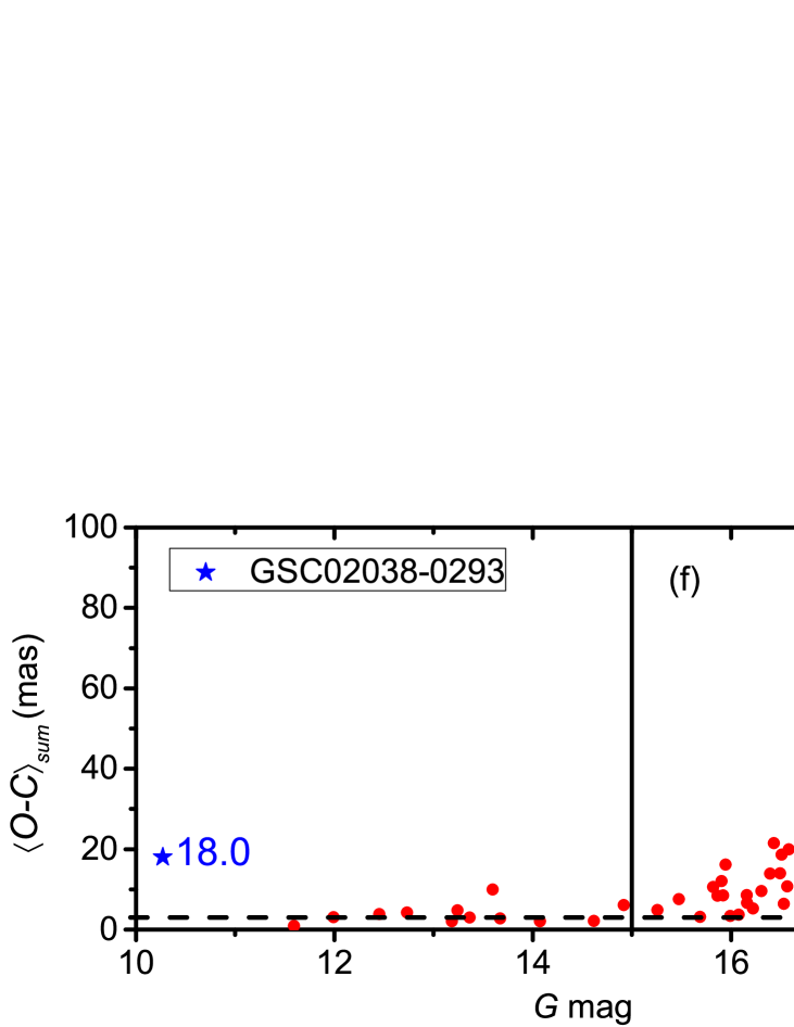
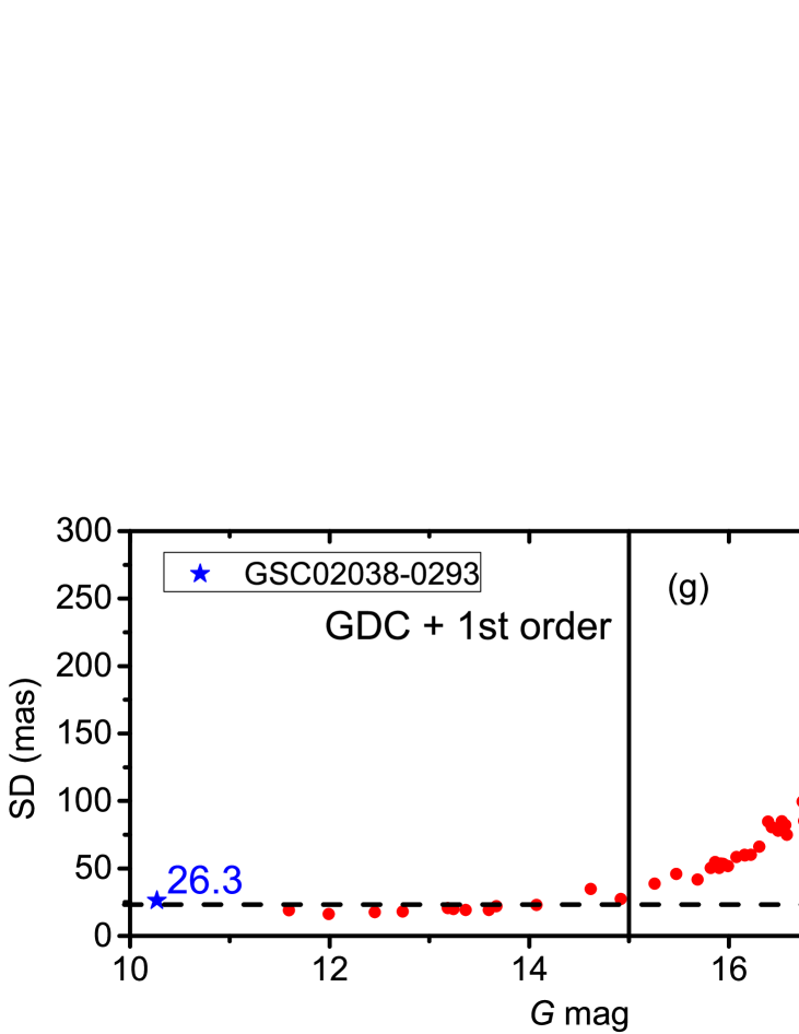
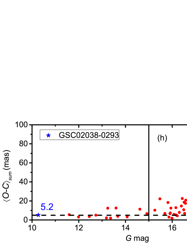
Figure 7: Comparison of the positional SD and mean $(O-C)$ obtained by using different methods for reduction. From top to bottom in this figure are the results of reduction using 1st, 2nd and 3rd-order plate constants, as well as the results obtained by reduction using the six-parameter plate constants after GD correction. The left panels show the mean $(O-C)$ for each star, while the right panels present the corresponding positional SD. The numbers in the panels are the statistics of the target GSC02038-00293. The horizontal dashed line marks the median of the positional SD or mean $(O-C)$ in each panel for stars brighter than 15 magnitude.

Empirically, when using the weighted least squares method to determine the plate constants for data reduction, the number of bright reference stars should be approximately 1.5 times the number of fitting parameters. This is crucial when determining the necessity of a GD solution.

5 Conclusions

We investigated a GD correction method based on the high-precision Gaia catalogue. The major advantage of this method is easy to implement. It was found that no more than fifteen frames, with only a dozen bright stars per frame, are enough to derive the accurate GD solution. As fitting errors are eliminated by averaging the coefficients from multiple frames, the final GD solution does not have overfitting issues even if only a dozen bright stars can be used to solve the high-order polynomial. To evaluate the accuracy of our GD solution, observations of open clusters taken with the 1-m and 2.4-m telescopes at Yunnan Observatory were reduced. In the reduction, our GD solution and a well-established GD solution (Peng et al., 2012; Wang et al., 2019) were used for GD correction, respectively. The results demonstrate that both methods achieve the same precision. In addition, the mean $(O-C)$ difference between our results and the reference results is only 1 mas for the YNO 1-m telescope observations and 2 mas for the YNO 2.4-m telescope observations. It is evident that our GD solution is convenient and effective.

This method presents significant value for some observations, such as those in which GD correction is unattainable due to the absence of relevant calibration data. This situation often occurs when dealing with historical observations, which are captured by the telescopes employed for photometric purposes. Because of the new research focus, astrometric analysis for these observations may become important. The observations of the binary GSC02038-00293 taken with the YNO 60-cm telescope are an example that satisfies the situation. By applying our GD solution in the reduction, the astrometric results of this target were significantly improved, with the mean $(O-C)$ decreased from 36 mas to 5 mas. The J6 observations in a sparse FOV taken with the YNO 2.4-m telescope were also corrected by the method, and the astrometric results of the target has been improved to some extent. Performance of our method in the processing of observations affected by large magnitude of GD, such as the Bok telescope observations (Zheng et al., 2022; Peng et al., 2023), will be discussed in the future.

References

- Anderson et al. (2006) Anderson, J., Bedin, L. R., Piotto, G., Yadav, R. S., & Bellini, A. 2006, A&A, 454, 1029, doi: \hrefhttp://doi.org/10.1051/0004-6361:20065004\nolinkurl10.1051/0004-6361:20065004
- Anderson & King (2003) Anderson, J., & King, I. R. 2003, PASP, 115, 113, doi: \hrefhttp://doi.org/10.1086/345491\nolinkurl10.1086/345491
- Bellini & Bedin (2009) Bellini, A., & Bedin, L. R. 2009, PASP, 121, 1419, doi: \hrefhttp://doi.org/10.1086/649061\nolinkurl10.1086/649061
- Bellini & Bedin (2010) —. 2010, A&A, 517, A34, doi: \hrefhttp://doi.org/10.1051/0004-6361/200913783\nolinkurl10.1051/0004-6361/200913783
- Bernard et al. (2018) Bernard, A., Neichel, B., Mugnier, L. M., & Fusco, T. 2018, MNRAS, 473, 2590, doi: \hrefhttp://doi.org/10.1093/mnras/stx2517\nolinkurl10.1093/mnras/stx2517
- Casetti-Dinescu et al. (2021) Casetti-Dinescu, D. I., Girard, T. M., Kozhurina-Platais, V., et al. 2021, PASP, 133, 064505, doi: \hrefhttp://doi.org/10.1088/1538-3873/abf32c\nolinkurl10.1088/1538-3873/abf32c
- Dal et al. (2012) Dal, H. A., Sipahi, E., & Özdarcan, O. 2012, PASA, 29, 150, doi: \hrefhttp://doi.org/10.1071/AS12007\nolinkurl10.1071/AS12007
- Gaia Collaboration et al. (2023) Gaia Collaboration, Vallenari, A., Brown, A. G. A., et al. 2023, A&A, 674, A1, doi: \hrefhttp://doi.org/10.1051/0004-6361/202243940\nolinkurl10.1051/0004-6361/202243940
- Green (1985) Green, R. M. 1985, Spherical Astronomy
- Illingworth et al. (2013) Illingworth, G. D., Magee, D., Oesch, P. A., et al. 2013, ApJS, 209, 6, doi: \hrefhttp://doi.org/10.1088/0067-0049/209/1/6\nolinkurl10.1088/0067-0049/209/1/6
- Lin et al. (2019) Lin, F. R., Peng, J. H., Zheng, Z. J., & Peng, Q. Y. 2019, MNRAS, 490, 4382, doi: \hrefhttp://doi.org/10.1093/mnras/stz2871\nolinkurl10.1093/mnras/stz2871
- Lin et al. (2020) Lin, F. R., Peng, Q. Y., & Zheng, Z. J. 2020, MNRAS, 498, 258, doi: \hrefhttp://doi.org/10.1093/mnras/staa2439\nolinkurl10.1093/mnras/staa2439
- McKay & Kozhurina-Platais (2018) McKay, M., & Kozhurina-Platais, V. 2018, WFC3/IR: Time Dependency of Linear Geometric Distortion, Instrument Science Report WFC3 2018-9, 11 pages
- Peng et al. (2017) Peng, H. W., Peng, Q. Y., & Wang, N. 2017, MNRAS, 467, 2266, doi: \hrefhttp://doi.org/10.1093/mnras/stx229\nolinkurl10.1093/mnras/stx229
- Peng & Fan (2010) Peng, Q., & Fan, L. 2010, Chinese Science Bulletin, 55, 791, doi: \hrefhttp://doi.org/10.1007/s11434-010-0053-2\nolinkurl10.1007/s11434-010-0053-2
- Peng et al. (2012) Peng, Q. Y., Vienne, A., Zhang, Q. F., et al. 2012, AJ, 144, 170, doi: \hrefhttp://doi.org/10.1088/0004-6256/144/6/170\nolinkurl10.1088/0004-6256/144/6/170
- Peng et al. (2023) Peng, X., Qi, Z., Zhang, T., et al. 2023, AJ, 165, 172, doi: \hrefhttp://doi.org/10.3847/1538-3881/acbc78\nolinkurl10.3847/1538-3881/acbc78
- Reid & Menten (2007) Reid, M. J., & Menten, K. M. 2007, ApJ, 671, 2068, doi: \hrefhttp://doi.org/10.1086/523085\nolinkurl10.1086/523085
- Service et al. (2016) Service, M., Lu, J. R., Campbell, R., et al. 2016, PASP, 128, 095004, doi: \hrefhttp://doi.org/10.1088/1538-3873/128/967/095004\nolinkurl10.1088/1538-3873/128/967/095004
- Wang et al. (2017) Wang, N., Peng, Q. Y., Peng, H. W., et al. 2017, MNRAS, 468, 1415, doi: \hrefhttp://doi.org/10.1093/mnras/stx550\nolinkurl10.1093/mnras/stx550
- Wang et al. (2019) Wang, N., Peng, Q. Y., Zhou, X., Peng, X. Y., & Peng, H. W. 2019, MNRAS, 485, 1626, doi: \hrefhttp://doi.org/10.1093/mnras/stz459\nolinkurl10.1093/mnras/stz459
- Zang et al. (2022) Zang, L., Qian, S., Zhu, L., & Liu, L. 2022, MNRAS, 511, 553, doi: \hrefhttp://doi.org/10.1093/mnras/stac047\nolinkurl10.1093/mnras/stac047
- Zhai et al. (2018) Zhai, C., Shao, M., Saini, N. S., et al. 2018, AJ, 156, 65, doi: \hrefhttp://doi.org/10.3847/1538-3881/aacb28\nolinkurl10.3847/1538-3881/aacb28
- Zheng et al. (2021) Zheng, Z. J., Peng, Q. Y., & Lin, F. R. 2021, MNRAS, 502, 6216, doi: \hrefhttp://doi.org/10.1093/mnras/stab406\nolinkurl10.1093/mnras/stab406
- Zheng et al. (2022) Zheng, Z. J., Peng, Q. Y., Vienne, A., Lin, F. R., & Guo, B. F. 2022, A&A, 661, A75, doi: \hrefhttp://doi.org/10.1051/0004-6361/202141725\nolinkurl10.1051/0004-6361/202141725