Forecasting and Backtesting Gradient Allocations of Expected Shortfall

Capital allocation is a procedure for quantifying the contribution of each source of risk to aggregated risk. The gradient allocation rule, also known as the Euler principle, is a prevalent rule of capital allocation under which the allocated capital captures the diversification benefit of the marginal risk as a component of overall risk. This research concentrates on Expected Shortfall (ES) as a regulatory standard and focuses on the gradient allocations of ES, also called ES contributions. We achieve the comprehensive treatment of backtesting the tuple of ES contributions in the framework of the traditional and comparative backtests based on the concepts of joint identifiability and multi-objective elicitability. For robust forecast evaluation against the choice of scoring function, we further develop Murphy diagrams for ES contributions as graphical tools to check whether one forecast dominates another under a class of scoring functions. Finally, leveraging the recent concept of multi-objective elicitability, we propose a novel semiparametric model for forecasting dynamic ES contributions based on a compositional regression model. In an empirical analysis of stock returns we evaluate and compare a variety of models for forecasting dynamic ES contributions and demonstrate the outstanding performance of the proposed model.

Keywords: Capital allocation; Compositional data analysis; Elicitability; Euler principle; Expected shortfall.

1 Introduction

Risk aggregation and risk allocation are two important procedures for financial risk management. The total risk of a portfolio or a financial institution is quantified in the first stage of risk aggregation, where financial regulation may require the use of certain risk measures, such as value-at-risk (VaR) and expected shortfall (ES). Due to some deficiencies of VaR, ES has become a standard risk measure in banking regulation (BCBS 2016, 2019). Since ES is coherent and particularly subadditive, it provides an incentive to diversify the risks in a financial institution or a portfolio. On the other hand, this is not the case for VaR, which discourages its use in risk aggregation. Readers may refer to Emmer et al. (2015) and McNeil et al. (2015) for a comprehensive discussion on VaR and ES in financial risk management.

Capital allocation is a second stage for quantifying the contribution of each source of risk to total risk. Reflecting the diversification benefit, the allocated capital to each component is calculated so that the sum of the allocated capital over all components equals the total capital. Among various allocation rules proposed in the literature, the Euler principle is a prevalent allocation rule justified from various perspectives, such as RORAC (return on risk-adjusted capital) compatibility (Tasche 1999), cooperative game theory (Denault 2001), and axiomatic foundation of capital allocations (Kalkbrener 2005); see also Tasche (2008) and references therein. Together with the growing importance of ES in recent banking regulations, this paper focuses on the situation of capital allocation when total risk is measured by ES and allocated capital is calculated under the Euler principle; see Section 2.1 for details. We call the allocated capital calculated in this setting ES contribution.

The rare event nature of the above tail risk quantities poses challenges in their statistical estimation and model evaluation. Forecast evaluation of tail risk quantities is called backtesting in financial terminology. Regarding these issues, elicitability and identifiability are important concepts of risk functionals, where elicitability allows for a comparative study of forecasting models, and identifiability offers an absolute criterion of forecast accuracy. These notions are also beneficial for estimating and calibrating models of tail risk quantities; see Nolde and Ziegel (2017). It is known that VaR is elicitable and identifiable by itself, whereas ES is elicitable and identifiable when it is simultaneously estimated with VaR (Fissler and Ziegel 2016). These results open the door to a semiparametric estimation of risk measures based on scoring functions; see, for example, Patton et al. (2019) and Taylor (2019).

In contrast to the backtesting of risk measures, studies on backtesting of dynamic capital allocation are quite limited in the literature. Bielecki et al. (2020) propose a backtesting method of ES contributions based on the concept called fairness. This method is essentially treated in the more general framework of calibration and traditional backtests introduced in Nolde and Ziegel (2017). Despite the usefulness of such traditional backtests for model validation, Nolde and Ziegel (2017) also point out several issues of such tests particularly in terms of model comparison and banking regulation. To this end, our first aim in this paper is to achieve the comprehensive treatment of backtesting ES contributions in the framework of traditional and comparative backtests (Nolde and Ziegel 2017) based on the concepts of joint identifiability and multi-objective elicitability (Fissler and Hoga 2023).

Although the results shown in Fissler and Hoga (2023) are on systemic risk measures such as CoVaR, CoES and MES, in Section 2.2 we translate their results under the setting of capital allocation. Summarizing their results in our setting, ES contributions are jointly identifiable with total VaR (i.e., VaR of the aggregated loss); moreover, ES contributions themselves are not elicitable, but are multi-objective elicitable, when combined with total VaR and with respect to the lexicographical order. The last statement means more precisely that the tuple of true ES contributions and total VaR is elicited as a unique minimizer of an expectation of some $\mathbb{R}^{2}$-valued scoring function with respect to the order on $\mathbb{R}^{2}$ such that the forecast evaluation of VaR is prioritized, and that of ES contributions is conducted secondarily. Therefore, in the framework of a comparative backtest based on multi-objective elicitability it is necessary to forecast ES contributions together with total VaR, and two forecasts of ES contributions are comparable only when the corresponding forecasts of total VaR are equally accurate. Section 2.3 summarizes the framework of backtests of dynamic ES contributions. We also discuss order sensitivity of scoring functions of ES contributions, which addresses comparability of two misspecified forecasts.

When conducting a comparative backtest in practice, it may not always be clear which scoring function to use. In addition, the resulting forecast ranking can be sensitive to the choice of scoring functions (Patton 2020). To overcome these problems, a diagnostic tool called the Murphy diagram is explored in  Ehm et al. (2016) and Ziegel et al. (2020) for robust forecast evaluation against the choice of scoring function. Based on a mixture representation of the scoring function, the Murphy diagram is particularly useful for checking whether one forecast dominates another under a class of scoring functions.

As a second aim of this paper, we complement the framework of backtesting ES contributions by developing their Murphy diagrams. They serve as a visual, intuitive way to compare competing forecasting models, thereby making it easier to digest and make informed decisions based on their performance. Section 3 introduces Murphy diagrams of ES contributions and summarizes their properties.

Our last aim of the paper is to leverage the concept of multi-objective elicitability and introduce a novel semiparametric model of dynamic ES contributions. Section 4 proposes such a model, which combines the joint semiparametric estimation of the pair of total VaR and total ES with the compositional regression for modeling the dynamics of the proportions of total ES to each component of risk. Based on multi-objective elicitability of ES contributions, forecast accuracy of total VaR is first evaluated prior to that of ES contributions. In addition, risk allocation is conceptually a second stage in the risk management process after quantifying overall risk. This theoretical and practical two-stage procedure motivates us to first model the dynamics of the pair of total VaR and total ES and then estimate ES contributions through the proportion of each source of risk to total ES. Since the component-wise sum of the vector of proportions must equal $1$, we model its dynamics by the compositional regression, which is a multiple regression for such compositional data.

Note that Boonen et al. (2019) also apply compositional data analysis to the problem of capital allocation. They first estimate allocated capital from the losses under the assumption of normality and then fit and evaluate compositional regression models by regarding the set of normalized allocated capital as compositional data. One potential challenge of this procedure is that statistical error and model uncertainty reside not only in the compositional regression model, but also in the estimated allocated capital. To overcome this issue, we fit and evaluate compositional regression models based on a scoring function of ES contributions. Multi-objective elicitability of ES contributions allows us to quantify the accuracy of compositional regression models based on realized losses and not on estimated allocated capital. The major advantage of our proposed semiparametric model is in the complete separation of modeling ES contributions from that of total VaR and total ES. This feature enables us to concentrate on modeling ES contributions based on the best existing model for the pair of total VaR and total ES and to assess the forecast accuracy of ES contributions among the proposed compositional regression models and an existing one by equalizing their total VaR and total ES.

For the remaining sections and appendices, Section 5 conducts an empirical analysis of a portfolio of stock returns and demonstrates superior performance of the proposed model compared with other models including those with conditional heteroskedastic volatilities, hysteretic effects, and time-varying correlations. Section 6 discusses potential directions for future research. We defer all technical results to Section S1, where references starting with the prefix “S” refer to the supplementary material. We also present details and additional results of our empirical analysis in Section S2.

2 Backtesting of ES contributions

2.1 Gradient allocations of expected shortfall

Throughout the paper we treat all vectors as row vectors and add the superscript $\top$ to indicate a column vector or the transpose of a matrix. In addition, we fix an atomless probability space $(\Omega,{\cal A},\mathbb{P})$, where all random objects are defined. For $p\in\{0\}\cup[1,\infty)$ and $d\in\mathbb{N}$, let ${\cal L}^{p}(\mathbb{R}^{d})$ be the set of all $\mathbb{R}^{d}$-value random vectors on $(\Omega,{\cal F},\mathbb{P})$ whose components have a finite $p$th moment. Let $F_{\bm{X}}$ be the joint cumulative distribution function (cdf) of $\bm{X}\in{\cal L}^{0}(\mathbb{R}^{d})$. We also define the collection ${\cal F}^{p}(\mathbb{R}^{d})=\{F_{\bm{X}}:\bm{X}\in{\cal L}^{p}(\mathbb{R}^{d})\}$ for $p\in\{0\}\cup[1,\infty)$ and $d\in\mathbb{N}$. Denote by ${\cal F}_{\text{c}}^{p}(\mathbb{R}^{d})$ the class of cdfs $F$ with a strictly positive Lebesgue density for every $\bm{x}\in\mathbb{R}^{d}$ such that $F(\bm{x})\in(0,1)$. Analogously, ${\cal L}_{\text{c}}^{p}(\mathbb{R}^{d})$ denotes the set of $\mathbb{R}^{d}$-valued random vectors whose cdf belongs to ${\cal F}_{\text{c}}^{p}(\mathbb{R}^{d})$. For $X\in{\cal L}^{0}(\mathbb{R})$, Value-at-Risk (VaR) with a confidence level $\alpha\in(0,1)$ is $\operatorname{VaR}_{\alpha}(X)=\inf\{x\in\mathbb{R}:F_{X}(x)\geq\alpha\}$. Moreover, for $X\in{\cal L}^{1}(\mathbb{R})$, the expected shortfall (ES) with a confidence level $\alpha\in(0,1)$ is $\operatorname{ES}_{\alpha}(X)=\frac{1}{1-\alpha}\int_{\alpha}^{1}\operatorname{VaR}_{\beta}(X){\rm d}\beta$, which coincides with $\operatorname{ES}_{\alpha}(X)=\mathbb{E}[X|X\geq\operatorname{VaR}_{\alpha}(X)]$ if $X\in\mathcal{L}_{\text{c}}^{1}(\mathbb{R})$. The confidence level $\alpha$ is typically chosen to be close to $1$, such as $0.975$ and $0.99$. Let $\bm{X}=(X_{1},\dots,X_{d})\in{\cal L}^{0}(\mathbb{R}^{d})$ be a random vector standing for the collection of losses to a portfolio or a financial institution. Moreover, let $S=X_{1}+\cdots+X_{d}$ be the total loss. Our sign convention is that positive values are losses and negative values are profits.

Under the prevalent Euler principle, the contribution of each component $X_{j}$, $j=1\dots,d$, to the risk of the total loss $\operatorname{ES}_{\alpha}(S)$ is determined by the gradient $\frac{\partial}{\partial\lambda_{j}}\operatorname{ES}_{\alpha}(\bm{\lambda}^{\top}\bm{X})|_{\bm{\lambda}=\mathbf{1}_{d}}$ provided that the partial derivative exists, where $\bm{\lambda}=(\lambda_{1},\dots,\lambda_{d})\in\mathbb{R}^{d}$ and $\mathbf{1}_{d}=(1,\dots,1)\in\mathbb{R}^{d}$. Given certain smoothness conditions (Tasche 1999), this derivative leads to:

$$\operatorname{ESC}_{\alpha}(X_{j},S)=\mathbb{E}[X_{j}|S\geq\operatorname{VaR}_{\alpha}(S)],$$ (1)

which we call the ES contribution for the $j$th risk. Note that the ES contribution itself is well-defined for $(X_{j},S)\in{\cal L}^{1}(\mathbb{R}^{2})$ without smoothness assumptions. If $S\in\mathcal{L}_{\text{c}}^{1}(\mathbb{R})$, then the following full allocation property holds:

$$\sum_{j=1}^{d}\operatorname{ESC}_{\alpha}(X_{j},S)=\operatorname{ES}_{\alpha}(S),$$ (2)

for which the total capital $\operatorname{ES}_{\alpha}(S)$ is allocated to $d$ components by the $d$-tuple of allocated capital:

$$\operatorname{ESC}_{\alpha}(\bm{X},S)=(\operatorname{ESC}_{\alpha}(X_{1},S),\dots,\operatorname{ESC}_{\alpha}(X_{d},S)).$$

For a generic $k$-dimensional risk functional $\bm{\varrho}\in\{\operatorname{VaR}_{\alpha},\operatorname{ES}_{\alpha},\operatorname{ESC}_{\alpha}\}^{k}$, we write $\bm{\varrho}(F)$ for $\bm{\varrho}(\bm{X})$, $\bm{X}\sim F$, by the law-invariance of $\bm{\varrho}$.

2.2 Multi-objective elicitability and joint identifiability of ES contributions

We introduce several properties required for backtesting ES contributions. Let ${\cal F}\subseteq{\cal F}^{0}(\mathbb{R}^{d})$, $k,\,m\in\mathbb{N}$, and $A\subseteq\mathbb{R}^{k}$. A function $\mathbf{S}:A\times\mathbb{R}^{d}\rightarrow\mathbb{R}^{m}$ is called $\mathcal{F}$-integrable if, for every $F\in\mathcal{F}$ and $\bm{r}\in A$, every component of the function $\bm{x}\mapsto\mathbf{S}(\bm{r},\bm{x})$ is integrable with respect to $F$. A functional $\bm{\varrho}:{\cal F}\rightarrow A$ is called multi-objective elicitable on ${\cal F}$ with respect to a total order $\preceq$ on $\mathbb{R}^{m}$ if there exists an $\mathcal{F}$-integrable function $\mathbf{S}:A\times\mathbb{R}^{d}\rightarrow\mathbb{R}^{m}$ such that, for every $F\in{\cal F}$, $\bm{\varrho}(F)$ is the unique minimizer of $\bm{r}\mapsto\mathbb{E}[\mathbf{S}(\bm{r},\bm{X})]$, $\bm{X}\sim F$, over $A$. The function $\mathbf{S}$ is called a (strictly $\mathcal{F}$-consistent multi-objective) scoring function for $\bm{\varrho}$. We simply call $\bm{\varrho}$ elicitable when a scoring function can be taken with $m=1$.

A functional $\bm{\varrho}:{\cal F}\rightarrow A$ is called identifiable on ${\cal F}$ if there exists an $\mathcal{F}$-integrable function $\mathbf{V}:A\times\mathbb{R}^{d}\rightarrow\mathbb{R}^{m}$ such that, for every $F\in{\cal F}$, $\bm{\varrho}(F)$ is the unique solution to the equation $\mathbb{E}[\mathbf{V}(\bm{r},\bm{X})]=\mathbf{0}_{m}$, $\bm{X}\sim F$, in terms of $\bm{r}$ on $A$. The function $\mathbf{V}$ is called a (strict $\mathcal{F}$-) identification function for $\bm{\varrho}$.

For $j\in\{1,\dots,d\}$, the $j$th ES contribution (1) coincides with the marginal expected shortfall (MES) of $(S,X_{j})$ considered in Fissler and Hoga (2023) provided that $(S,X_{j})\in\mathcal{F}_{\text{c}}^{1}(\mathbb{R}^{2})$. This observation immediately yields the following results on the multi-objective elicitability and joint identifiability of ES contributions shown in Theorem 4.2 and Theorem S.3.1 of  Fissler and Hoga (2023), respectively. In the following, the lexicographic order $\leq_{\text{lex}}$ is adopted as a total order on $\mathbb{R}^{2}$. For every $(a_{1},b_{1}),(a_{2},b_{2})\in\mathbb{R}^{2}$, we write $(a_{1},b_{1})\leq_{\text{lex}}(a_{2},b_{2})$ if $a_{1}<a_{2}$ or if $(a_{1}=a_{2}\text{ and }b_{1}\leq b_{2})$. Moreover, we define:

$$\tilde{\mathcal{F}}_{\text{c}}^{1}(\mathbb{R}^{d})=\left\{F\in\mathcal{F}^{1}(\mathbb{R}^{d}):F_{X_{j},S}\in{\cal F}_{\text{c}}^{1}(\mathbb{R}^{2})\text{ for }\bm{X}\sim F\text{ and }S=\sum_{j=1}^{d}X_{j}\right\}.$$ (3)

Proposition 1.

Let $\alpha\in(0,1)$ and $\mathcal{F}\subseteq\tilde{\mathcal{F}}_{\text{c}}^{1}(\mathbb{R}^{d})$.

1. For every $j\in\{1,\dots,d\}$, the pair $F_{\bm{X}}\mapsto(\operatorname{ESC}_{\alpha}(F_{X_{j},S}),\operatorname{VaR}_{\alpha}(F_{S}))$ is multi-objective elicitable on $\mathcal{F}$ with respect to $(\mathbb{R}^{2},\leq_{\text{lex}})$. A strictly $\mathcal{F}$-consistent multi-objective scoring function $\mathbf{S}_{j}:\mathbb{R}^{2}\times\mathbb{R}^{d}\rightarrow(\mathbb{R}^{2},\leq_{\text{lex}})$ is given by:

   $$\mathbf{S}_{j}((m_{j},v),\bm{x}) =(\operatorname{S}^{\text{VaR}}(v,s),\operatorname{S}_{j}^{\text{ESC}}((m_{j},v),\bm{x})),$$

   $$\operatorname{S}^{\text{VaR}}(v,s)=\{\mathbbm{1}{\{s\leq v\}}-\alpha\}\{h(v)-h(s)\},$$

   $$\operatorname{S}_{j}^{\text{ESC}}((m_{j},v),\bm{x})=\mathbbm{1}{\{s>v\}}\left\{\phi_{j}^{\prime}(m_{j})(m_{j}-x_{j})-\phi_{j}(m_{j})+\phi_{j}(x_{j})\right\},$$

   where $s=\sum_{i=1}^{d}x_{i}$, $h:\mathbb{R}\rightarrow\mathbb{R}$ is a strictly increasing function, and $\phi_{j}:\mathbb{R}\rightarrow\mathbb{R}$ is a strictly convex function with subgradient $\phi_{j}^{\prime}$ such that $\mathbf{S}_{j}$ is $\mathcal{F}$-integrable.

2. The $(d+1)$-tuple $F_{\bm{X}}\mapsto(\operatorname{ESC}_{\alpha}(F_{\bm{X},S}),\operatorname{VaR}_{\alpha}(F_{S}))$ is multi-objective elicitable on $\mathcal{F}$ with respect to $(\mathbb{R}^{2},\leq_{\text{lex}})$. A strictly $\mathcal{F}$-consistent multi-objective scoring function $\mathbf{S}:\mathbb{R}^{d+1}\times\mathbb{R}^{d}\rightarrow(\mathbb{R}^{2},\leq_{\text{lex}})$ is given by:

   $$\mathbf{S}((\bm{m},v),\bm{x})=\left(\operatorname{S}^{\text{VaR}}(v,s),\sum_{j=1}^{d}\operatorname{S}_{j}^{\text{ESC}}((m_{j},v),\bm{x})\right),$$

   where $\operatorname{S}^{\text{VaR}}$ and $\operatorname{S}_{j}^{\text{ESC}}$, $j=1,\dots,d$, are as defined in (S1).

Proposition 2.

Let $\alpha\in(0,1)$ and $\mathcal{F}\subseteq\tilde{\mathcal{F}}_{\text{c}}^{1}(\mathbb{R}^{d})$.

1. For every $j\in\{1,\dots,d\}$, the pair $F_{\bm{X}}\mapsto(\operatorname{ESC}_{\alpha}(F_{X_{j},S}),\operatorname{VaR}_{\alpha}(F_{S}))$ is identifiable on $\mathcal{F}$ with a strict $\mathcal{F}$-identification function $\mathbf{V}_{j}:\mathbb{R}^{2}\times\mathbb{R}^{d}\rightarrow\mathbb{R}^{2}$ given by:

   $$\mathbf{V}_{j}((m_{j},v),\bm{x}) =(\operatorname{V}^{\text{VaR}}(v,s),\operatorname{V}_{j}^{\text{ESC}}((m_{j},v),\bm{x})),$$

   $$\operatorname{V}^{\text{VaR}}(v,s)=\alpha-\mathbbm{1}{\{s\leq v\}},$$

   $$\operatorname{V}_{j}^{\text{ESC}}((m_{j},v),\bm{x})=\mathbbm{1}{\{s>v\}}(x_{j}-m_{j}).$$

2. The $(d+1)$-tuple $F_{\bm{X}}\mapsto(\operatorname{ESC}_{\alpha}(F_{\bm{X},S}),\operatorname{VaR}_{\alpha}(F_{S}))$ is identifiable on $\mathcal{F}$ with a strict $\mathcal{F}$-identification function $\mathbf{V}:\mathbb{R}^{d+1}\times\mathbb{R}^{d}\rightarrow\mathbb{R}^{d+1}$ given by:

   $$\mathbf{V}((\bm{m},v),\bm{x}) =(\operatorname{V}^{\text{VaR}}(v,s),\operatorname{V}_{1}^{\text{ESC}}((m_{1},v),\bm{x}),\dots,\operatorname{V}_{d}^{\text{ESC}}((m_{d},v),\bm{x})),$$

   where $\operatorname{V}^{\text{VaR}}$ and $\operatorname{V}_{j}^{\text{ESC}}$, $j=1,\dots,d$, are as defined in (V1).

Remark 1.

To simplify the notation and subsequent discussion, in Proposition 1 we specialize the form of scoring function originally obtained in Theorem 4.2 of  Fissler and Hoga (2023). For instance, we take a specific auxiliary function in $\operatorname{S}^{\text{VaR}}$ so that $\operatorname{S}^{\text{VaR}}$ is independent of $x$ and equal to the scoring function of VaR presented in Equation (5) of Ehm et al. (2016).

As a concrete example of the scoring functions in Proposition 1, the choice $h(s)=s$ in $\operatorname{S}^{\text{VaR}}$ yields the well-known pinball loss $\operatorname{S}^{\text{VaR}}(v,s)=(\mathbbm{1}{\{s\leq v\}}-\alpha)(v-s)$, and $\phi_{j}(x)=x^{2}$ in $\operatorname{S}_{j}^{\text{ESC}}$ leads to the square loss $\operatorname{S}_{j}^{\text{ESC}}((m_{j},v),\bm{x})=\mathbbm{1}\{s>v\}(x_{j}-m_{j})^{2}$; see Nolde and Ziegel (2017) and Fissler and Hoga (2023) for more examples.

2.3 Backtesting dynamic ES contributions

We introduce a setting for estimating dynamic ES contributions. Let $\{\bm{X}_{t}\}_{t\in\mathbb{N}}$, $\bm{X}_{t}=(X_{1,t},\dots,X_{d,t})$, be a series of losses of interest, which is adapted to the filtration ${\cal G}=\{{\cal G}_{t}\}_{t\in\mathbb{N}}$. For $S_{t}=X_{1,t}+\cdots+X_{d,t}$, let $VaR_{t}$ and $ES_{t}$ be VaR and ES of $S_{t}|{\cal G}_{t-1}$, respectively, with the prescribed confidence level $\alpha$. For $j=1,\dots,d$, the ES contribution of $X_{j,t}$ to $S_{t}$ given ${\cal G}_{t-1}$ is denoted by $ESC_{j,t}$.

We introduce a generic notation $\bm{\varrho}_{t}$ for the pair $(ESC_{j,t},VaR_{t})$ for a fixed $j\in\{1,\dots,d\}$, or the $(d+1)$-tuple $(ESC_{1,t},\dots,ESC_{d,t},VaR_{t})$. Let $\{\hat{\bm{\varrho}}_{t}\}_{t\in\mathbb{N}}$ and $\{\hat{\bm{\varrho}}_{t}^{\ast}\}_{t\in\mathbb{N}}$ be two series of predictions of $\{\bm{\varrho}_{t}\}_{t\in\mathbb{N}}$, which are $\mathcal{G}$-predictable. We assume that $\tilde{\mathcal{F}}_{\text{c}}^{1}(\mathbb{R}^{d+1})$ in (3) contains all distributions of $(\bm{X}_{t},S_{t})$ and $(\bm{X}_{t},S_{t})|\mathcal{G}_{t-1}$ almost surely. The multi-objective elicitability and identifiability presented in Section 2.2 enable the conduct of comparative backtests and traditional backtests (calibration tests) based on the following statistics:

$$\mathbf{\bar{S}}(\hat{\bm{\varrho}}) =\frac{1}{|\mathbb{T}_{\text{out}}|}\sum_{t\in\mathbb{T}_{\text{out}}}\mathbf{S}(\hat{\bm{\varrho}}_{t},\bm{X}_{t}),$$

$$\mathbf{\bar{V}}(\hat{\bm{\varrho}}) =\frac{1}{|\mathbb{T}_{\text{out}}|}\sum_{t\in\mathbb{T}_{\text{out}}}\mathbf{V}(\hat{\bm{\varrho}}_{t},\bm{X}_{t}),$$

with $\mathbf{\bar{S}}(\hat{\bm{\varrho}}^{\ast})$ and $\mathbf{\bar{V}}(\hat{\bm{\varrho}}^{\ast})$ defined analogously, where $\mathbf{S}$ is a multi-objective scoring function for $\bm{\varrho}$, $\mathbf{V}$ is an identification function for $\bm{\varrho}$, and $\mathbb{T}_{\text{out}}$ is the out-of-sample period $\mathbb{T}_{\text{out}}$ such that we forecast and backtest $\{\bm{\varrho}_{t}\}_{t\in\mathbb{T}_{\text{out}}}$. In practice, we divide a given finite sample period $\mathbb{T}=\{1,\dots,n+T\}$ into the in-sample period $\mathbb{T}_{\text{in}}=\{1,\dots,n\}$ and the out-of-sample period $\mathbb{T}_{\text{out}}=\{n+1,\dots,n+T\}$. For each $t\in\mathbb{T}_{\text{out}}$, we forecast $\bm{\varrho}_{t}$ at $t-1$ based on the past $n$ observations of $\{\bm{X}_{t-s}\}_{s\in\mathbb{T}_{\text{in}}}$.

Comparative backtests of ES contributions concern whether some order between $\mathbf{\bar{S}}(\hat{\bm{\varrho}})$ and $\mathbf{\bar{S}}(\hat{\bm{\varrho}}^{\ast})$ is statistically supported, and one-step and two-step approaches are proposed due to multi-objective elicitability with respect to the lexicographical order; see Section 5 of Fissler and Hoga (2023) for details. A key property of scoring functions regarding the comparative backtests is order sensitivity, which addresses comparability of two misspecified forecasts. We defer some technical discussion on this property in Section S1.2. To summarize it briefly, the average scores of the two misspecified forecasts of ES contributions are ordered when (1) the corresponding total VaRs are ordered (in the component-wise sense in Definition 3.1 of Fissler and Ziegel (2019)), or (2) the misspecified total VaRs are equal (in this case, $\operatorname{S}_{1}^{\text{ESC}},\dots,\operatorname{S}_{d}^{\text{ESC}}$ elicit biased ES contributions), the two misspecified ES contributions are ordered in the component-wise sense, and they are not between the true and biased ES contributions. Regarding Case (2), misspecification of the total VaR produces intervals such that multiple forecasts of ES contributions belonging there have inconsistent orders of average scores.

In traditional backtests of ES contributions, we seek statistical evidence on the signs of $\mathbf{\bar{V}}(\hat{\bm{\varrho}})$ and $\mathbf{\bar{V}}(\hat{\bm{\varrho}}^{\ast})$; see Section 2.2 of Nolde and Ziegel (2017) for details. It is useful to associate the sign of $\mathbf{\bar{V}}$ with over- and under-estimations of ES contributions. This is because under-estimation of risk functionals is considered to be more problematic than over-estimation from a regulatory viewpoint. With the identification functions in Proposition 2, we have, for $\bm{X}\in\mathcal{F}$, that $\mathbb{E}[\operatorname{V}^{\text{VaR}}(v,S)]\leq 0$ if and only if $\operatorname{VaR}_{\alpha}(S)\leq v$; i.e., the forecast $v$ over-estimates the total VaR. Moreover, under the correct specification $v=\operatorname{VaR}_{\alpha}(S)$ and for $j\in\{1,\dots,d\}$, a forecast $m_{j}\in\mathbb{R}$ of the $j$th ES contribution is over-estimated; i.e., $\operatorname{ESC}_{\alpha}(X_{j},S)\leq m_{j}$, if and only if $\mathbb{E}[\operatorname{V}_{j}^{\text{ESC}}((m_{j},v),\bm{X})]\leq 0$.

3 Robust forecast evaluation of ES contributions

To conduct a comparative backtest as presented in Section 2.3, we select a (multi-objective) scoring function from the class of functions characterized in Proposition 1. This is also required when we estimate models via score minimization, which we will consider in Section 4. Such a dependence of the risk measurement procedure on the choice of scoring function complicates the fair evaluation of forecasts. Patton (2020) also shows that forecast rankings can be sensitive to the choice of scoring function.

To overcome this issue, Ehm et al. (2016) propose a diagnostic tool for evaluating multiple forecasts called the Murphy diagram, which is based on a mixture representation of a relevant class of scoring functions. According to Theorem 1 of Ehm et al. (2016), $\operatorname{S}^{\text{VaR}}$ in Proposition 1 admits the mixture representation $\operatorname{S}^{\text{VaR}}(v,s)=\int_{\mathbb{R}}\operatorname{S}_{\eta}^{\text{VaR}}(v,s)\mathrm{d}H(\eta)$ for a non-negative measure $H$, where $\operatorname{S}_{\eta}^{\text{VaR}}:\mathbb{R}\times\mathbb{R}\rightarrow\mathbb{R}$, defined by:

$$\operatorname{S}_{\eta}^{\text{VaR}}(v,s)=(\mathbbm{1}{\{s<v\}}-\alpha)(\mathbbm{1}{\{\eta<v\}}-\mathbbm{1}{\{\eta<s\}}),\quad\eta\in\mathbb{R},$$ (4)

is called an elementary scoring function for VaR. For competing forecasts $\{\widehat{VaR}_{t}^{(\ell)}\}_{t\in\mathbb{T}_{\text{out}}}$, $\ell=1,\dots,L$, of VaRs, a Murphy diagram displays the curves:

$$\eta\mapsto\frac{1}{|\mathbb{T}_{\text{out}}|}\sum_{t\in\mathbb{T}_{\text{out}}}\operatorname{S}_{\eta}^{\text{VaR}}\left(\widehat{VaR}_{t}^{(\ell)},s_{t}\right),\quad\ell=1,\dots,L,$$

against $\eta$. The diagram is negatively oriented in the sense that forecasts with lower curves are evaluated to be more accurate.

The next proposition provides mixture representations of the scoring functions for ES contributions presented in Proposition 1.

Proposition 3.

1. Fix $j\in\{1,\dots,d\}$. The scoring function $\operatorname{S}_{j}^{\text{ESC}}$ in Proposition 1 (S1) admits the mixture representation:

   $$\operatorname{S}_{j}^{\text{ESC}}((m_{j},v),\bm{x})=\int_{\mathbb{R}}\operatorname{S}_{j,\eta}^{\text{ESC}}((m_{j},v),\bm{x})\,\mathrm{d}H_{j}(\eta),$$ (5)

   where $H_{j}$ is a non-negative measure satisfying $\mathrm{d}H_{j}(\eta)=\mathrm{d}\phi_{j}^{\prime}(\eta)$, $\eta\in\mathbb{R}$, and $\operatorname{S}_{j,\eta}^{\text{ESC}}:\mathbb{R}^{2}\times\mathbb{R}^{d}\rightarrow\mathbb{R}$ is defined by:

   $$\operatorname{S}_{j,\eta}^{\text{ESC}}((m_{j},v),\bm{x})=\begin{cases}\mathbbm{1}{\{s>v\}}(x_{j}-\eta),&\text{ if }m_{j}\leq\eta<x_{j},\\ \mathbbm{1}{\{s>v\}}(\eta-x_{j}),&\text{ if }x_{j}\leq\eta<m_{j},\\ 0,&\text{ otherwise}.\\ \end{cases}$$ (6)

2. The scoring function $\operatorname{S}^{\text{ESC}}$ in Proposition 1 (S2), with $\phi_{j}=\cdots=\phi_{d}=:\phi$, admits the mixture representation:

   $$\operatorname{S}^{\text{ESC}}((\bm{m},v),\bm{x})=\int_{\mathbb{R}}\operatorname{S}_{\eta}^{\text{ESC}}((\bm{m},v),\bm{x})\,\mathrm{d}H(\eta),$$ (7)

   where $H$ is a non-negative measure satisfying $\mathrm{d}H(\eta)=\mathrm{d}\phi^{\prime}(\eta)$, $\eta\in\mathbb{R}$, and $\operatorname{S}_{\eta}^{\text{ESC}}:\mathbb{R}^{2}\times\mathbb{R}^{d}\rightarrow\mathbb{R}$ is defined by:

   $$\operatorname{S}_{\eta}^{\text{ESC}}((\bm{m},v),\bm{x})=\sum_{j=1}^{d}\operatorname{S}_{j,\eta}^{\text{ESC}}((m_{j},v),\bm{x}).$$

The elementary scoring function (6) can be interpreted as a degree of regret in the following setting. Suppose that the $j$th branch of a company has fixed capital $\eta$ to cover a future loss, whose point forecast is denoted by $m_{j}$, incurred at this branch under the specific situation when the company incurs a loss greater than $v$. If $m_{j}\leq\eta$, then the branch expects that the initial capital can cover a future loss. In this case, since an excess loss $(x_{j}-\eta)$ is incurred when the realized loss $x_{j}$ exceeds $\eta$ and $s>v$ occurs, the amount $\operatorname{S}_{j,\eta}^{\text{ESC}}((m_{j},v),\bm{x})=\mathbbm{1}{\{s>v\}}(x_{j}-\eta)_{+}$ can be understood as a degree of regret against the initial expectation. If $\eta<m_{j}$, then the branch expects that the initial capital does not cover a future loss, and thus some risk treatment can be conducted. In this case, the branch realizes the squandered opportunity of capital reduction $(\eta-x_{j})_{+}$ when $s>v$ occurs, and thus the degree of regret against the initial expectation can be measured by $\operatorname{S}_{j,\eta}^{\text{ESC}}((m_{j},v),\bm{x})=\mathbbm{1}{\{s>v\}}(\eta-x_{j})_{+}$. Provided $v=\operatorname{VaR}_{\alpha}(S)$, the true $j$th ES contribution is the optimal $m_{j}$ minimizing the expected degree of regret.

Since $\phi_{j}$ and $\phi$ in (M1) and (M2) above are strictly convex, the corresponding measures $H_{j}$ and $H$ assign positive mass to any finite interval on $\mathbb{R}$. Note that $\mathrm{d}H(x)=2\mathrm{d}x$ for the square loss, and $\operatorname{S}_{j,\eta}^{\text{ESC}}$ arises from $\operatorname{S}_{j}^{\text{ESC}}$ in Proposition 1 (S1) by taking $\phi_{j}(x)=(x-\eta)_{+}$, although this function is not strictly convex.

Based on the mixture representations (5) and (7), a Murphy diagram of ES contributions can be drawn analogously to the case of VaR. For $l\in\{1,\dots,L\}$, let:

$$\{\hat{\bm{\varrho}}_{t}^{(\ell)}\}_{t\in\mathbb{T}_{\text{out}}},\quad\text{where}\quad\hat{\bm{\varrho}}_{t}=(\widehat{ESC}_{1,t}^{(\ell)},\dots,\widehat{ESC}_{d,t}^{(\ell)},\widehat{VaR}_{t}^{(\ell)}),$$

be a series of predictions in the setting of Section 2.3. The Murphy diagram of the $j$th ES contribution displays the curves.

$$\eta\mapsto\bar{\operatorname{S}}_{j,\eta}^{\text{ESC}}(l):=\frac{1}{|\mathbb{T}_{\text{out}}|}\sum_{t\in\mathbb{T}_{\text{out}}}\operatorname{S}_{j,\eta}^{\text{ESC}}((\widehat{ESC}_{j,t}^{(\ell)},\widehat{VaR}_{t}^{(\ell)}),\bm{x}_{t}),\quad\ell=1,\dots,L.$$

The Murphy diagram of the $d$-tuple of ES contributions analogously exhibits $\eta\mapsto\bar{\operatorname{S}}_{\eta}^{\text{ESC}}(l):=\sum_{j=1}^{d}\bar{\operatorname{S}}_{j,\eta}^{\text{ESC}}(l)$ for $\ell=1,\dots,L$. We obtain these curves and their differences on the whole real line by evaluating them on a finite set. This is because $\bar{\operatorname{S}}_{j,\eta}^{\text{ESC}}(l)$ and $\bar{\operatorname{S}}_{\eta}^{\text{ESC}}(l)$ are piecewise linear functions of $\eta$ with all kinks and jump points contained in $\mathcal{D}_{j}^{(l)}=\{x_{j,t},\widehat{ESC}_{j,t}^{(\ell)},t\in\mathbb{T}_{\text{out}}\}$ and $\mathcal{D}^{(l)}=\bigcup_{j=1}^{d}\mathcal{D}_{j}^{(l)}$, respectively. Moreover, $\bar{\operatorname{S}}_{j,\eta}^{\text{ESC}}(l)$ and $\bar{\operatorname{S}}_{\eta}^{\text{ESC}}(l)$ vanish outside of $[\min(\mathcal{D}_{j}^{(l)}),\max(\mathcal{D}_{j}^{(l)})]$ and $[\min(\mathcal{D}^{(l)}),\max(\mathcal{D}^{(l)})]$, respectively.

We note that Murphy diagrams of ES contributions depend on the corresponding forecast of total VaR. Therefore, as naturally induced from multi-objective elicitability, a completely fair evaluation among multiple forecasts of ES contributions can be conducted when their corresponding forecasts of total VaR are all equal. In such a case, more advanced analyses, such as forecast dominance tests proposed by Ziegel et al. (2020), are available.

4 Proposed models for estimating dynamic ES contributions

Pprevious sections have shown that clear and rigid comparison among forecasting models of ES contributions is accessible among those with equal total VaRs. In this section we exploit this feature and propose a new model based on compositinal regression.

According to the evaluation criterion based on multi-objective elicitability of ES contributions, forecast accuracy of total VaR is of utmost importance since estimated ES contributions are compared only for models estimating total VaRs with equal accuracy. As considered in Dimitriadis and Hoga (2023), this valuation principle naturally encourages a two-stage approach, where we first model the dynamics of $\{VaR_{t}\}$, possibly induced from the dynamics of $\{S_{t}\}$, and then consider the dynamics of ES contributions, which may also be induced from the dynamics of $\{(X_{j},S_{t})\}$ for $j=1,\dots,d$. We call this a top-down approach and summarize its benefits and limitations in Section S2.1. In this approach the dynamics of $\{ES_{t}\}$ can also be estimated together with $\{VaR_{t}\}$ in the first stage due to the natural order in the risk measurement procedure and, more importantly, joint elicitability of $(\operatorname{VaR}_{\alpha},\operatorname{ES}_{\alpha})$, where ES_α can be elicited only in combination with VaR_α (Fissler and Ziegel 2016). An alternative approach is to specify the dynamics of $\{\bm{X}_{t}\}$, which we call a bottom-up approach. This approach may be discouraged in terms of the two-stage forecast evaluation since total VaR is modeled only indirectly; see Section S2.1 for more details of this approach.

Despite the appeals of the top-down approach in forecasting ES contributions, special attention is required in this approach so that the empirical counterpart of the full allocation property $\sum_{j=1}^{d}\widehat{ESC}_{j,t}=\widehat{ES}_{t}$ is satisfied. To handle this constraint, we propose a new model for estimating dynamic ES contributions. In what follows, we describe our proposed procedure for the case of one-step ahead forecast, where we use the losses $\{\bm{X}_{t}\}_{t\in\mathbb{T}_{\text{in}}}$, $\mathbb{T}_{\text{in}}=\{1,\dots,n\}$, to forecast ES contributions at time $n+1$.

The proposed model consists of two stages, where the dynamics of total ES are first estimated in combination with that of total VaR, and then ES contributions are estimated from the proportion of the total ES to each component of risk. In the first stage, we estimate the dynamics of $(ES_{t},VaR_{t})$ for $t\in\mathbb{T}_{\text{in}}$ and then forecast $(VaR_{n+1},ES_{n+1})$ based on this estimated dynamics. For this purpose, various models are proposed in the literature; see, for example, Patton et al. (2019), Taylor (2019) and Taylor (2022). Joint elicitability of the pair of risk measures $(\operatorname{VaR}_{\alpha},\operatorname{ES}_{\alpha})$ enables us to estimate the joint dynamics of this pair by score minimization; see, for example, Taylor (2019). In this paper we do not specify any specific model in this stage and instead select the best model based on the currently available information and candidate models. Denote by $(\widehat{VaR}_{t},\widehat{ES}_{t})_{t\in\mathbb{T}}$, $\mathbb{T}=\{1,\dots,n+1\}$, the dynamics forecasted in this stage.

In the second stage, we allocate $\widehat{ES}_{t}$ to each component of risk with the weight vector $\bm{w}_{t}=(w_{1,t},\dots,w_{d,t})\in[0,1]^{d}$, $\sum_{j=1}^{d}w_{j,t}=1$, such that $ESC_{j,t}=w_{j,t}\times ES_{t}$. For all $j=1,\dots,d$ and $t\in\mathbb{T}$, we assume that $0<w_{j,t}<1$, which is implied by the natural assumption that $0<ESC_{j,t}<ES_{t}$. Consequently, the weight vector $\bm{w}_{t}$ lies in $\mathcal{S}_{d}=\left\{\bm{w}\in(0,1)^{d}:\sum_{j=1}^{d}w_{j}=1\right\}$. Data on $\mathcal{S}_{d}$ are called compositional data, and statistical modeling of such data has been extensively studied in the literature; see Aitchison (1982); Aitchison and J. Egozcue (2005); Pawlowsky-Glahn and Buccianti (2011); and references therein. A common approach for modeling compositional data is first transforming the data to an unconstrained space to eliminate the sum constraint and then constructing a model on the unconstrained space.

One of the most prominent examples of such a transform is the isometric logratio transformation (ilr, Egozcue et al. 2003) defined by:

$$\operatorname{ilr}(\bm{w})=V^{\top}\ln(\bm{w})\in\mathbb{R}^{d-1},\quad\bm{w}\in\mathcal{S}_{d},$$

where $V\in\mathbb{R}^{d\times(d-1)}$ is a given matrix such that $V^{\top}V=I_{d-1}$, $VV^{\top}=I_{d}-\frac{1}{d}\mathbf{1}_{d}\mathbf{1}_{d}^{\top}$ and $V^{\top}\mathbf{1}_{d}=\mathbf{0}_{d-1}$. Matrix $V$ is called the contrast matrix. The inverse map of $\operatorname{ilr}$ is given by:

$$\operatorname{ilr}^{-1}(\bm{z})=\operatorname{C}(\exp(V\bm{z}))\in\mathcal{S}_{d},\quad\bm{z}\in\mathbb{R}^{d-1},$$ (8)

where $\operatorname{C}:\mathbb{R}^{d}\rightarrow\mathcal{S}_{d}$ is the closing operator defined by:

$$\operatorname{C}(\bm{x})=\frac{\bm{x}}{\mathbf{1}_{d}^{\top}\bm{x}},\quad\bm{x}\in\mathbb{R}^{d}.$$

Note that the map $\operatorname{ilr}$ depends on the choice of $V$, and we fix this matrix so that the resulting transform yields:

$$\operatorname{ilr}_{k}(\bm{w})=\sqrt{\frac{d-k}{d-k+1}}\ln\left(\frac{w_{k}}{\left(\prod_{l=k+1}^{d}w_{l}\right)^{1/(d-k)}}\right),\quad k=1,\dots,d-1.$$

With this choice of $V$, $\operatorname{ilr}_{k}(\bm{w})$, $k\in\{1,\dots,d-1\}$, can be interpreted as a balance between the $k$th weight and the sum of the weights over the assets $k+1,\dots,d$. Note that $0$ and $1$ cannot be included in the compositional data for the above transformations to be well-defined. This well-known limitation of ilr does not cause a significant problem in our analysis since $0$ or $1$ in the allocated weights corresponds to the practically irrelevant case when no capital or full capital is allocated to one asset, respectively.

We consider the following generic model on the dynamics of the allocation weights $\{\bm{w}_{t}\}_{t\in\mathbb{T}}$:

$$\bm{w}_{t+1} =\upsilon_{\bm{\theta}}(\bm{w}_{t},\bm{X}_{t}):=\operatorname{ilr}^{-1}\left(\bm{\tau}+\bm{\Phi}\operatorname{ilr}(\bm{w}_{t})+\bm{\Psi}\bm{Y}_{t}\right),\quad t\in\mathbb{T},$$ (9)

where $\bm{Y}_{t}$ is a $q$-dimensional random vector representing a vector of covariates, and $\bm{\theta}=(\bm{\tau},\bm{\Phi},\bm{\Psi})$ is a set of parameters on $\Theta$ such that $\bm{\tau}\in\mathbb{R}^{d-1}$, $\bm{\Phi}\in\mathbb{R}^{(d-1)\times(d-1)}$, and $\bm{\Psi}\in\mathbb{R}^{(d-1)\times q}$. The initial weight $\bm{w}_{1}$ can also be regarded as a parameter to be estimated or as a constant determined by some external information. We then estimate parameters in (9) by minimizing the average score of the $d$-tuple of ES contributions in Proposition 1 (S2) with $\phi_{1}=\cdots=\phi_{d}=:\phi$, $\phi(x)=x^{2}$:

$$\hat{\bm{\theta}}=\operatorname{argmin}_{\bm{\theta}\in\Theta}\sum_{t\in\mathbb{T}_{\text{in}}}\sum_{j=1}^{d}\left\{x_{j,t}-\upsilon_{\bm{\theta}}(\bm{w}_{t},\bm{x}_{t})_{j}\widehat{ES}_{t}\right\}^{2}\mathbbm{1}{\left\{s_{t}>\widehat{VaR}_{t}\right\}},$$ (10)

where $\bm{x}_{t}=(x_{1,t},\dots,x_{d,t})$ and $s_{t}$ are the realizations of $\bm{X}_{t}$ and $S_{t}$, respectively, and $\widehat{VaR}_{t}$ and $\widehat{ES}_{t}$ are the estimates given in the first stage. Once the estimated parameter $\hat{\bm{\theta}}$ is obtained, we forecast the ES contributions at time $n+1$ by ${\widehat{ESC}}_{j,n+1}=\hat{w}_{j,n+1}\widehat{ES}_{n+1}$, $j=1,\dots,d$, where $\hat{\bm{w}}_{1}=\bm{w}_{1}$ and $\hat{\bm{w}}_{t+1}=\upsilon_{\hat{\mathbf{\theta}}}(\hat{\bm{w}}_{t},\bm{X}_{t})$, $t=1,\dots,n$. Note that the estimated weight $\hat{\bm{w}}_{n+1}$ belongs to $\mathcal{S}_{d}$, which ensures the full allocation property $\sum_{j=1}^{d}\widehat{ESC}_{j,t}=\widehat{ES}_{t}$.

5 Empirical study

Various models in the literature are available to forecast ES contributions. In this section we compare them with our proposed model in Section 4 in the traditional and comparative backtests introduced in Section 2.3 and based on the Murphy diagrams introduced in Section 3. We first describe the setting and models in comparison in Section 5.1. We then show results of the forecast evaluation in Section 5.2. Finally, we discuss forecast accuracy of the compared models in Section 5.3.

5.1 Setting and model description

We consider a portfolio consisting of the following $d=3$ stock prices with equal weights: Amazon (AMZN), Alphabet Class A (GOOGL), and Telsa (TSLA). From 2010-06-30 to 2023-05-30, each series consists of $n+T=3249$ negative daily log returns multiplied by $100$. We conduct a rolling window analysis with window size $n=2249$ and forecast day-ahead ES contributions for the last $T=1000$ observations. Namely, for $t=n+1,\dots,n+T$, we forecast total VaR, total ES, and ES contributions of $\bm{X}_{t}|\mathcal{G}_{t-1}$ based on the past $n$ observations $\{\bm{X}_{s}\}_{s\in\{t-n,\dots,t-1\}}$. Following the Fundamental Review of the Trading Book (FRTB), we focus on the confidence levels $\alpha=0.975$ (BCBS 2013).

In this analysis we compare $6$ models including the proposed one in Section 4. We briefly introduce these models here and defer a detailed description to Section S2.2. As a simple benckmark, our first model is the historical simulation (HS) model, where at each time $t$ we estimate the risk functional $\bm{\varrho}_{t}=(ESC_{1,t},\dots,ESC_{d,t},VaR_{t},ES_{t})$ nonparametrically based on the past $n$ observations. Second, we consider what we call the bottom-up GARCH (GARCH.BU) model, where estimates of the risk functionals are induced from a copula-GARCH model (Jondeau and Rockinger 2006; Huang et al. 2009) among $\{\bm{X}_{t}\}$. To compare the bottom-up and top-down approaches, we also consider the top-down GARCH (GARCH.TD) model, where we fit $d$ number of bivariate copula-GARCH models on $\{(X_{j,t},S_{t})\}$, $j=1,\dots,d$. Since the above three models do not take the hysteresis effect and time-varying correlations into account, our fourth model is the bivariate hysteretic autoregressive model with GARCH error and dynamic conditional correlations  (HAR.GARCH,  Chen et al. 2019), fitted to $\{(X_{j,t},S_{t})\}$, $j=1,\dots,d$, in the top-down approach. Following (2), total ES is estimated as the sum of estimated ES contributions.

We next include two compositional regression models in our comparison. These models share the estimates $\{\widehat{VaR}_{t},\widehat{ES}_{t}\}$, which are obtained by an AR-GARCH model on $\{S_{t}\}$. Our fifth model is termed the compositional regression model with least square estimation (CR.LSE). In this model we follow Boonen et al. (2019) and first estimate a series of ES contributions under the assumption that each $\bm{X}_{t}|\mathcal{G}_{t-1}$ follows an elliptical distribution. We then transform this series by (8) to obtain the allocation weights $\{\hat{\bm{w}}_{t}\}\subset\mathcal{S}_{d}$. By regarding this set of allocation weights as compositional data, we fit the compositional regression model (9) by the standard least square estimation. Finally, our sixth model is the compositional regression model based on score minimization (CR.OPT), which is the proposed model described in Section 4. We choose the vector of covariates $\bm{Y}_{t}=\left(\operatorname{ilr}\circ\operatorname{C}\left(\max(\bm{X}_{t}S_{t},\bm{\epsilon})\right),\operatorname{ilr}\circ\operatorname{C}\left(-\min(\bm{X}_{t}S_{t},-\bm{\epsilon})\right)\right)$, where $\bm{\epsilon}=(0.01,\dots,0.01)\in\mathbb{R}^{d}$ is a $d$-vector of small numbers, and $\max$ and $\min$ are applied component-wise. The term $\bm{X}_{t}S_{t}=(X_{1,t}S_{t},\dots,X_{d,t}S_{t})$ is motivated by the fact that the allocation weight $\bm{w}_{t}$ equals $\operatorname{C}(\mathbb{E}[\bm{X}_{t}S_{t}|{\cal G}_{t-1}])$ when $\bm{X}_{t}|{\cal G}_{t-1}$ follows an elliptical distribution with zero vector of location parameters. Therefore, we regard the corresponding regression coefficients of $\bm{Y}_{t}$ as the positive and negative effects of the recent covariance term between $\bm{X}_{t}$ and $S_{t}$ to the balance among allocation weights. We introduce $\bm{\epsilon}$ to ensure that all the components of $\max(\bm{X}_{t}S_{t},\bm{\epsilon})$ and $\min(\bm{X}_{t}S_{t},-\bm{\epsilon})$ are non-zero. For the initial allocation weight $\bm{w}_{1}$, we use the compositional data $\hat{\bm{w}}_{1}$ generated in CR.LSE.

In Section S2.3 we display the estimated dynamics of total VaR, total ES, and ES contributions on the out-of-sample period $\mathbb{T}_{\text{out}}$ together with the realized losses. In summary, we observe that HS only captures the average trends, HAR.GARCH tends to estimate ES contributions lower than others, and CR.OPT typically leads to more fluctuated estimates. Compared with these three models, the other three models seem to produce estimates relatively similar with each other.

5.2 Model evaluation

We conduct the comparative and traditional backtests in the two-step approach. In Section S2.4 we also conduct those in the one-step approach (Fissler and Hoga 2023). For the comparative backtests, we follow Section 2.3 of Nolde and Ziegel (2017) and conduct the Diebold-Mariano (DM)-tests (Diebold and Mariano 1995) for the series of score differences. For an HAC estimator (Andrews 1991) in the test statistic, we choose the Bartlett kernel (Newey and West 1987) with the automatic bandwidth estimator based on AR(1) approximation; see Section 6 of Andrews (1991). In the context of Nolde and Ziegel (2017), we choose CR.OPT for the benchmark model and compare other models as internal models. Consequently, in the three-zone approach of Fissler et al. (2016), the red region indicating superiority of CR.OPT over a compared model is statistically supported, the green region shows that CR.OPT is inferior to the alternative model, and the yellow region means that further investigation is required since there is no statistical evidence on the order between the two models. We fix the significance level to be $0.05$. We repeat this analysis for total VaR, total ES, tuple of ES contributions, and $j$th ES contribution for $j=1,\dots,d$. For the scoring functions, we choose the pinball loss for VaR, AL log score (Taylor 2019) for ES, and square loss for tuple of ES contributions, as well as each of them. Tables 1 and 2 report the average scores and p-values of the one-sided and two-sided DM-tests, based on which we obtain the regions in the three-zone approach.

Table 1: Results of the DM-tests to compare the forecast accuracy of total VaR, total ES, and tuple of ES contributions with CR.OPT as the benchmark model.

	Average scorea	Rankb	p-valuec			Regiond
H0			$=$ CR.OPT	$\leq$ CR.OPT	$\geq$ CR.OPT
(1) Total VaR
HS	56.038	6	0.008	0.996	0.004	red
GARCH.BU	48.016	5	0.225	0.888	0.112	yellow
GARCH.TD	46.780	3	0.200	0.900	0.100	yellow
HAR.GARCH	46.885	4	0.871	0.565	0.435	yellow
CR.LSE	46.721	1.5	—-	—-	—-	—-
CR.OPT	46.721	1.5	—-	—-	—-	—-
(2) Total ES
HS	423.005	6	0.003	0.998	0.002	red
GARCH.BU	393.304	5	0.426	0.787	0.213	yellow
GARCH.TD	391.345	1	0.697	0.348	0.652	yellow
HAR.GARCH	392.767	4	0.653	0.673	0.327	yellow
CR.LSE	391.436	2.5	—-	—-	—-	—-
CR.OPT	391.436	2.5	—-	—-	—-	—-
(3) Tuple of ES contributions
HS	189.216	6	0.004	0.998	0.002	red
GARCH.BU	115.213	4	0.062	0.969	0.031	red
GARCH.TD	97.073	3	0.426	0.787	0.213	yellow
HAR.GARCH	124.779	5	0.135	0.932	0.068	yellow
CR.LSE	95.256	2	0.432	0.784	0.216	yellow
CR.OPT	85.428	1	—-	—-	—-	—-

• ^aAverage scores are multiplied by $100$.

• ^bRanks are based on average scores.

• ^cThe p-values are calculated based on the three different null hypotheses, where “$=$ CR.OPT” means that the model is equally accurate as CR.OPT, and “$\leq$ ($\geq$) CR.OPT” represents the hypothesis that the model is less (more) accurate than CR.OPT.

• ^dResults of the three-zone approach are presented.

Table 2: Results of the DM-tests to compare the forecast accuracy of $j$th ES contribution, $j\in\{1,\dots,d\}$, with CR.OPT as the benchmark model. See the footnotes in Table 1 for details.

	Average score	Rank	p-value			Region
H0			$=$ CR.OPT	$\leq$ CR.OPT	$\geq$ CR.OPT
(1) ES contribution (AMZN)
HS	33.603	6	0.179	0.910	0.090	yellow
GARCH.BU	18.965	3	0.810	0.595	0.405	yellow
GARCH.TD	20.026	4	0.698	0.651	0.349	yellow
HAR.GARCH	13.351	1	0.579	0.289	0.711	yellow
CR.LSE	23.075	5	0.224	0.888	0.112	yellow
CR.OPT	17.438	2	—-	—-	—-	—-
(2) ES contribution (GOOGL)
HS	28.672	6	0.067	0.966	0.034	red
GARCH.BU	13.196	4	0.941	0.529	0.471	yellow
GARCH.TD	12.117	2	0.655	0.328	0.672	yellow
HAR.GARCH	15.629	5	0.364	0.818	0.182	yellow
CR.LSE	11.091	1	0.440	0.220	0.780	yellow
CR.OPT	13.005	3	—-	—-	—-	—-
(3) ES contribution (TSLA)
HS	126.941	6	0.018	0.991	0.009	red
GARCH.BU	83.052	4	0.035	0.982	0.018	red
GARCH.TD	64.930	3	0.377	0.812	0.188	yellow
HAR.GARCH	95.799	5	0.137	0.932	0.068	yellow
CR.LSE	61.090	2	0.490	0.755	0.245	yellow
CR.OPT	54.984	1	—-	—-	—-	—-

We next describe our traditional backtests. Denote by $\left(\widehat{ESC}_{1,t},\dots,\widehat{ESC}_{d,t},\widehat{VaR}_{t},\widehat{ES}_{t}\right)$, $t\in\mathbb{T}_{\text{out}}$, the tuple of forecasted risk functionals. For total VaR, let $\operatorname{V}_{t}^{\text{VaR}}=\operatorname{V}^{\text{VaR}}\left(\widehat{VaR}_{t},S_{t}\right)$, where $\operatorname{V}^{\text{VaR}}$ is as defined in Proposition 2. We construct the DM-type test statistic $\sqrt{T}\bar{\operatorname{V}}_{T}^{\text{VaR}}/\hat{\sigma}_{T}^{\text{VaR}}$, where $\bar{\operatorname{V}}_{T}^{\text{VaR}}=(1/T)\sum_{t=1}^{T}\operatorname{V}_{t}^{\text{VaR}}$, and $\hat{\sigma}_{T}^{\text{VaR}}$ is the HAC estimator of the standard deviation of $\sqrt{T}\bar{\operatorname{V}}_{T}^{\text{VaR}}$ as considered in the comparative backtests above. Following Section 2.2 of Nolde and Ziegel (2017), we use a normal distribution as a null distribution to test unconditional calibration, sub-calibration, and super-calibration, which are associated with precise estimation, over-estimation, and under-estimation, respectively, for this identification function of VaR; see Section 2.3. Following these relationships, we adopt the three-zone approach and say that the forecast model is in the red region if the null hypothesis of sub-calibration is rejected, in the green region if the null hypothesis of super-calibration is rejected, and in the yellow region if none of these hypotheses are rejected. For total ES, we replace $\operatorname{V}_{t}^{\text{VaR}}$ in the above analysis with $\operatorname{V}_{t}^{\text{ES}}=\operatorname{V}^{\text{ES}}\left((\widehat{VaR}_{t},\widehat{ES}_{t}),S_{t}\right)$, where:

$$\operatorname{V}^{\text{ES}}\left((v,e),s\right)=v-e-\frac{1}{1-\alpha}\mathbbm{1}\{s>v\}(v-s).$$

This identification function maintains the above relationships; see Section 2.2.2 of Nolde and Ziegel (2017). For $j$th ES contribution, $j\in\{1,\dots,d\}$, we replace $\operatorname{V}_{t}^{\text{VaR}}$ in the above analysis with $\operatorname{V}_{j,t}^{\text{ESC}}=\operatorname{V}_{j}^{\text{ESC}}\left((\widehat{ESC}_{j,t},\widehat{VaR}_{t}),\bm{X}_{t}\right)$, where $\operatorname{V}_{j}^{\text{ESC}}$ is as defined in Proposition 2. We report the results of these tests in Tables 3 and 4. Due to joint identifiability of total ES (see Section 2.1 of  Nolde and Ziegel 2017) and $j$th ES contribution for $j=1,\dots,d$ (see Proposition 2) in combination with total VaR, we also conduct Wald-tests for these risk quantities in the one-step approach; see Section S2.4 for details.

Table 3: Results of the DM-type tests to verify the forecast accuracy of total VaR and total ES.

	Average score	p-valuea			Regionb
H0		$=$ True	$\leq$ True	$\geq$ True
(1) Total VaR
HS	0.032	0.000	1.000	0.000	red
GARCH.BU	0.015	0.013	0.993	0.007	red
GARCH.TD	0.009	0.116	0.942	0.058	yellow
HAR.GARCH	0.011	0.057	0.971	0.029	red
CR.LSE	0.009	0.116	0.942	0.058	yellow
CR.OPT	0.009	0.116	0.942	0.058	yellow
(2) Total ES
HS	6.441	0.002	0.999	0.001	red
GARCH.BU	0.689	0.620	0.690	0.310	yellow
GARCH.TD	-0.073	0.949	0.474	0.526	yellow
HAR.GARCH	1.768	0.169	0.916	0.084	yellow
CR.LSE	0.508	0.652	0.674	0.326	yellow
CR.OPT	0.508	0.652	0.674	0.326	yellow

• ^aThe p-values are calculated based on the three different null hypotheses, where “$=$ True” means that the forecast is precise, “$\leq$ True” represents the hypothesis that the forecast is under-estimated, and “$\geq$ True” stands for the case when the forecast is over-estimated.

• ^b Results of the three-zone approach are presented.

Table 4: Results of the DM-type tests to verify the forecast accuracy of the $j$th ES contribution for $j=1,\dots,d$. See the footnotes in Table 3 for details.

	Average score	p-value			Region
H0		$=$ True	$\leq$ True	$\geq$ True
(1) ES contribution (AMZN)
HS	0.013	0.487	0.757	0.243	yellow
GARCH.BU	-0.005	0.742	0.371	0.629	yellow
GARCH.TD	-0.008	0.565	0.283	0.717	yellow
HAR.GARCH	0.032	0.005	0.998	0.002	red
CR.LSE	-0.009	0.541	0.271	0.729	yellow
CR.OPT	-0.012	0.363	0.182	0.818	yellow
(2) ES contribution (GOOGL)
HS	0.029	0.088	0.956	0.044	red
GARCH.BU	-0.004	0.731	0.366	0.634	yellow
GARCH.TD	-0.009	0.427	0.214	0.786	yellow
HAR.GARCH	0.043	0.001	1.000	0.000	red
CR.LSE	-0.008	0.474	0.237	0.763	yellow
CR.OPT	0.001	0.938	0.531	0.469	yellow
(3) ES contribution (TSLA)
HS	-0.009	0.803	0.401	0.599	yellow
GARCH.BU	-0.063	0.028	0.014	0.986	green
GARCH.TD	-0.023	0.365	0.183	0.817	yellow
HAR.GARCH	0.105	0.001	1.000	0.000	red
CR.LSE	-0.012	0.636	0.318	0.682	yellow
CR.OPT	-0.017	0.458	0.229	0.771	yellow

We finally visually check the performance of the forecasts by Murphy diagrams. For total VaR, the diagram is written based on (4); see Ehm et al. (2016) for details. We refer to Ziegel et al. (2020) for the Murphy diagram of ES. The Murphy diagram of the tuple of ES contributions is drawn based on Proposition 3 (M2). We also display Murphy diagrams of the $j$th ES contribution for $j=1,\dots,d$ based on Proposition 3 (M1). The results appear in Figure 1.

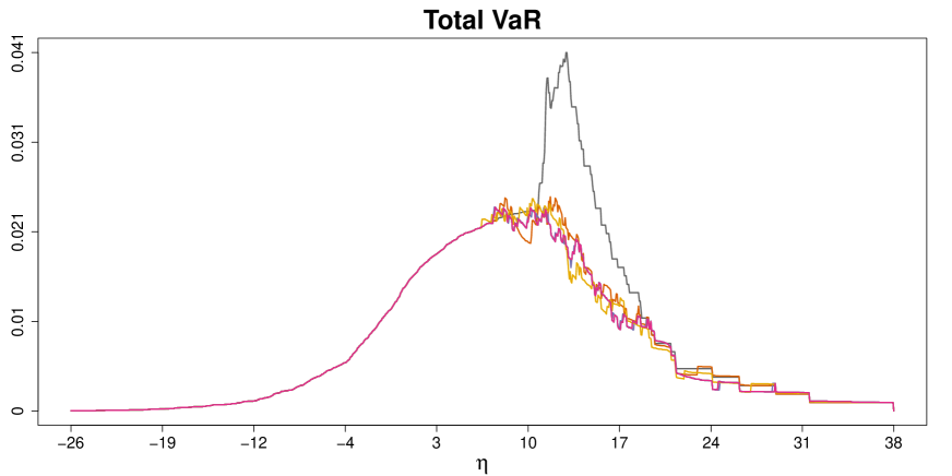
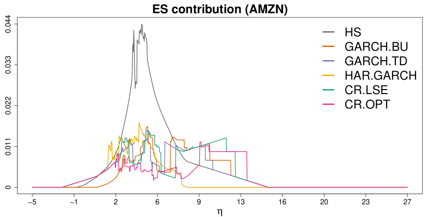
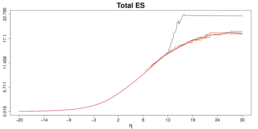
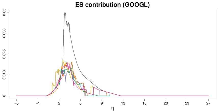
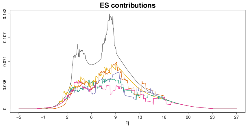
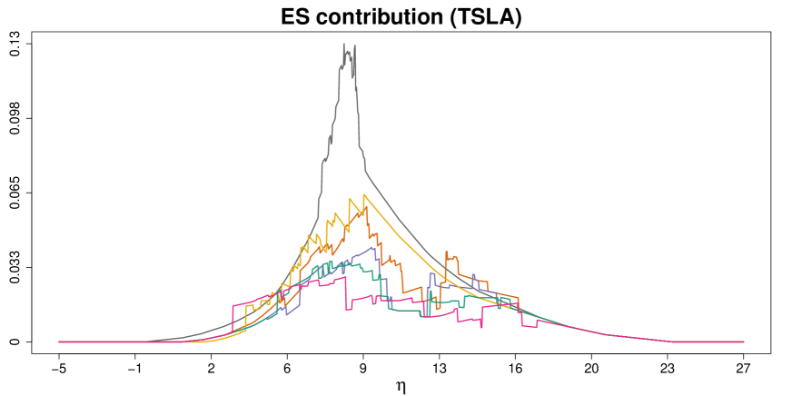
Figure 1: Murphy diagrams of total VaR, total ES, tuple of ES contributions, and each of them with confidence level of $0.975$ estimated by the $6$ models.

5.3 Discussion

According to the results of the comparative backtests in Tables 1 and 2, we first observe that HS is inferior to others in terms of average scores, which is detected by the red region in the three-zone approach only except for the ES contribution of AMZN. Moreover, CR.OPT tends to have lower scores than others and achieves the best performance for total VaR, tuple of ES contributions, and ES contribution of TSLA. Overall, GARCH.TD outperforms GARCH.BU, and HAR.GARCH does not perform well except for the ES contribution of AMZN. For total VaR in Table 1 (1), we observe the tendency that the forecasts of total VaR used in CR.LSE and CR.OPT are more accurate than others. Nevertheless, no test statistically supports the difference in the forecast accuracy of total VaRs except for HS, which justifies the forecast comparisons of ES contributions in terms of their scores.

In Table 1 (2) for total ES we find slightly lower performances of GARCH.BU and HAR.GARCH than others, which indicate that the top-down approach can be slightly more preferable than the bottom-up approach, and it may not be recommendable to estimate total ES indirectly as the sum of ES contributions. In addition to total ES, both of GARCH.BU and HAR.GARCH do not perform well for the tuple of ES contributions as well as each of them except for AMZN. For the case of AMZN, HAR.GARCH performs the best, which may imply the existence of the hysteretic effect and/or dynamic conditional correlations in the series of stock returns. From the perspective of multi-objective elicitability, we can directly compare the forecast accuracy of ES contributions between CR.OPT and CR.LSE since they share common forecasts of total VaR. We observe that CR.OPT outperforms CR.LSE for all the cases except the ES contribution of GOOGL. Finally, we see in Table S5 of Section S2.4 that the Wald-tests do not statistically support any additional orders among our compared models, which may not be surprising since no difference in the forecast accuracy of total VaRs is statistically verified other than HS.

We next check the results of the traditional backtests in Tables 3 and 4. Overall, the results are consistent with those of the comparative backtests, and HS is particularly not identified well. Other than HS, we find that GARCH.BU and HAR.GARCH are two models that typically fail the tests. For these models, the forecasts are often under-estimated except for the case that GARCH.BU over-estimates the ES contribution of TSLA. The other three models, GARCH.TD, CR.LSE, and CR.OPT, pass the traditional backtests. These results are consistent with those in Table S6 of Section S2.4. The only difference in this one-step approach is that the Wald-test for GARCH.TD rejects the null hypothesis of under-estimation of total ES with a correct specification of total VaR.

Since all the above results depend on the specific choices of scoring functions, it is beneficial to check the Murphy diagrams to diagnose the robustness of our observations for different choices of scoring functions. Overall, we do not observe any uniform dominance among the curves except HS, which is distinguishable for all the risk quantities. Compared with total VaR and total ES, larger differences are more visible for ES contributions. Particularly for the tuple of ES contributions and the ES contribution of TSLA, the curves of CR.OPT are typically lower, and those of GARCH.BU and HAR.GARCH tend to be higher. In addition, the curves are more tangled for ES contributions of AMZN and GOOGL. These differences are consistent with the fact that, from Table 2 and the y-axes of Murphy diagrams of ES contributions, TSLA has much larger contribution to the score of the tuple of ES contributions than AMZN and GOOGL have, and thus optimization in CR.OPT puts higher weight to the score of TSLA under the full allocation property.

6 Conclusion and outlook

We conduct traditional and comparative backtests for the gradient allocations of ES based on newly developed Murphy diagrams, which are robust diagnostic tools against the choice of scoring function. Moreover, motivated by the comparability of ES contributions in multi-objective elicitability and by the preservability of the full allocation property, we propose a novel semiparametric compositional regression model to estimate the tuple of ES contributions. Our empirical analysis demonstrates superior performance of our proposed model for forecasting ES contributions and the induced total ES. We believe that these results are of great benefit for portfolio and enterprise risk management in financial and regulatory applications.

We conclude this section by offering an outlook for future research on backtesting ES contributions. First, exploring theoretical aspects of our proposed compositional regression model, such as stability, consistency, and asymptotic normality, is of great interest. As a practical aspect, variable selection for our proposed model lies beyond the scope of the present paper. Second, in a future work it may be interesting to extend our estimation procedure of risk allocations to VaR contributions, the gradient allocation of VaR (see Gribkova et al. 2023; Koike et al. 2022, for recent works), and other capital allocation rules based on optimization (Dhaene et al. 2012; Maume-Deschamps et al. 2016; Koike and Hofert 2021).

Supplement to “Forecasting and Backtesting Gradient Allocations of Expected Shortfall”

Section S1 provides proofs and details of the technical statements in the main paper. Section S2 gives a for detailed description of the empirical analysis in the main paper as well as some additional results of backtesting in the one-step approach (Fissler and Hoga, 2023). Throughout the supplementary material, references starting with “S” refer to this supplement, and those without this prefix refer to the main paper.

Appendix S1 Technical details

S1.1 Proof of Proposition 3

(M2) is an immediate consequence of (M1), and thus it suffices to show (M1). We fix $j\in\{1,\dots,d\}$. For a strictly convex function $\phi_{j}:\mathbb{R}\rightarrow\mathbb{R}$ with subgradient $\phi_{j}^{\prime}$, define the Bregman-type function $\Phi_{j}:\mathbb{R}\times\mathbb{R}\rightarrow\mathbb{R}$ as:

$$\Phi_{j}(m,x)=\phi_{j}(x)-\phi_{j}(m)-\phi_{j}^{\prime}(m)(x-m).$$

Following the proof of Theorem 1 in Ehm et al. (2016), it holds that:

$$\Phi_{j}(m,x)=\int_{m}^{x}(x-\eta)\,\mathrm{d}\phi_{j}^{\prime}(\eta),\quad\text{ for $m,x\in\mathbb{R}$ such that }m<x.$$

Therefore, for $m\in\mathbb{R}$ and $\bm{x}=(x_{1},\dots,x_{d})\in\mathbb{R}^{d}$ such that $m<x_{j}$, we have that:

$$\operatorname{S}_{j}^{\text{ESC}}((m,v),\bm{x}) =\mathbbm{1}{\{s>v\}}\left\{\phi_{j}^{\prime}(m)(m-x_{j})-\phi_{j}(m)+\phi_{j}(x_{j})\right\}$$

$$=\mathbbm{1}{\{s>v\}}\Phi_{j}(m,x_{j})$$

$$=\int_{\mathbb{R}}\operatorname{S}_{j}^{\text{ESC}}((m,v),\bm{x})\,\mathrm{d}\phi_{j}^{\prime}(\eta).$$

This representation is shown to hold analogously for the case $m>x_{j}$ and is trivial for the case $m=x_{j}$.

S1.2 Order sensitivity

In this section we explore order sensitivity for ES contributions, which concerns whether two misspecified forecasts of ES contributions are ordered by means of the multi-objective scoring function in Proposition 1 if one tuple of forecasts is closer to the true ES contributions than another. The next proposition presents conditions under which two misspecified forecasts are ordered in this sense.

Proposition S4.

Let $\bm{X}\in\tilde{\mathcal{F}}_{\text{c}}^{1}(\mathbb{R}^{d})$. For $v\in\mathbb{R}$ and $j\in\{1,\dots,d\}$, denote by $\mathcal{I}_{j}(v)$ an open interval with endpoints $\operatorname{ESC}_{\alpha}(X_{j},S)$ and $\mathbb{E}[X_{j}|S>v]$.

1. Fix $j\in\{1,\dots,d\}$. Let $\mathbf{S}_{j}$ be a multi-objective scoring function in Proposition 1 (S1). For two misspecified forecasts $(m_{j},v),(m_{j}^{\ast},v^{\ast})\in\mathbb{R}^{2}$ of $(\operatorname{ESC}_{\alpha}(X_{j},S),\operatorname{VaR}_{\alpha}(S))$, we have that $\mathbb{E}[{\mathbf{S}}_{j}((m_{j},v),\bm{X})]\leq_{\text{lex}}\mathbb{E}[{\mathbf{S}}_{j}((m_{j}^{\ast},v^{\ast}),\bm{X})]$ if one of the following cases hold:

   1. $v^{\ast}<v\leq\operatorname{VaR}_{\alpha}(S)$;

   2. $\operatorname{VaR}_{\alpha}(S)\leq v<v^{\ast}$;

   3. $v=v^{\ast}$ and $m_{j}^{\ast}<m_{j}\leq\tilde{m}$ for all $\tilde{m}\in\mathcal{I}_{j}(v)$;

   4. $v=v^{\ast}$ and $\tilde{m}\leq m_{j}<m_{j}^{\ast}$ for all $\tilde{m}\in\mathcal{I}_{j}(v)$.

2. Let $\mathbf{S}$ be a multi-objective scoring function in Proposition 1 (S2). For two misspecified forecasts $(\bm{m},v),(\bm{m}^{\ast},v^{\ast})\in\mathbb{R}^{d+1}$ of $(\operatorname{ESC}_{\alpha}(\bm{X},S),\operatorname{VaR}_{\alpha}(S))$, we have that $\mathbb{E}[{\mathbf{S}}((\bm{m},v),\bm{X})]\leq_{\text{lex}}\mathbb{E}[{\mathbf{S}}((\bm{m}^{\ast},v^{\ast}),\bm{X})]$ if one of the following cases hold: (i); (ii); (iii) for all $j\in\{1,\dots,d\}$; (iv) for all $j\in\{1,\dots,d\}$.

Proof.

(O2) is a direct consequence from (O1), and thus we will show (O1) for a fixed $j\in\{1,\dots,d\}$. It is shown in Section 2.4  of Ehm et al. (2016) that $\mathbb{E}[\operatorname{S}^{\text{VaR}}(v,S)]<\mathbb{E}[\operatorname{S}^{\text{VaR}}(v^{\ast},S)]$ holds if (i) or (ii) holds. Therefore, each of (i) and (ii) implies $\mathbb{E}[{\mathbf{S}}_{j}((m_{j},v),\bm{X})]\leq_{\text{lex}}\mathbb{E}[{\mathbf{S}}_{j}((m_{j}^{\ast},v^{\ast}),\bm{X})]$.

We next suppose that (iii) holds. In this case, we have that $\mathbb{E}[S^{\text{VaR}}(v,S)]=\mathbb{E}[S^{\text{VaR}}(v^{\ast},S)]$. For any $\eta\in\mathbb{R}$ and $\bm{x}\in\mathbb{R}^{d}$, the elementary scoring function $\operatorname{S}_{j\eta}^{\text{ESC}}$ in Proposition 3 (M1) satisfies:

$$\operatorname{S}_{j,\eta}^{\text{ESC}}((m_{j}^{\ast},v),\bm{x})-\operatorname{S}_{j,\eta}^{\text{ESC}}((m_{j},v),\bm{x})=\mathbbm{1}{\{s>v\}}(x_{j}-\eta)(\mathbbm{1}{\{m_{j}^{\ast}\leq\eta\}}-\mathbbm{1}{\{m_{j}\leq\eta\}}),$$

and thus:

$$\mathbb{E}[\operatorname{S}_{j,\eta}^{\text{ESC}}((m_{j}^{\ast},v),\bm{X})] -\mathbb{E}[\operatorname{S}_{j,\eta}^{\text{ESC}}((m_{j},v),\bm{X})]$$

$$=\mathbb{P}(S>v)(\mathbb{E}[X_{j}|S>v]-\eta)(\mathbbm{1}{\{m_{j}^{\ast}\leq\eta\}}-\mathbbm{1}{\{m_{j}\leq\eta\}}),$$

which is nonnegative for all $\eta\in\mathbb{R}$ and positive for $m_{j}^{\ast}<\eta<m_{j}$. Since $H_{j}((m_{j}^{\ast},m_{j}))>0$, the mixture representation in Proposition 3 (M1) yields:

$$\mathbb{E}[\operatorname{S}_{j}^{\text{ESC}}((m_{j},v),\bm{X})]<\mathbb{E}[\operatorname{S}_{j}^{\text{ESC}}((m_{j}^{\ast},v^{\ast}),\bm{X})],$$

which implies $\mathbb{E}[{\mathbf{S}}_{j}((m_{j},v),\bm{X})]\leq_{\text{lex}}\mathbb{E}[{\mathbf{S}}_{j}((m_{j}^{\ast},v^{\ast}),\bm{X})]$. (iv) is shown analogously. ∎

Although various concepts of order sensitivity are proposed in Fissler and Ziegel (2019), we are not aware of any improvement on Proposition S4 except for some special cases; see Sections 3.3.1 and 3.3.2 of Fissler and Ziegel (2019) for related discussions.

Appendix S2 Details of the empirical analysis

In this section we describe details of the empirical analysis omitted in Section 5. For brevity, we describe models for the case when $\mathbb{T}_{\text{in}}=\{1,\dots,n\}$ and $\mathbb{T}_{\text{out}}=\{n+1\}$, and thus $\mathbb{T}=\{1,\dots,n+1\}$.

S2.1 Bottom-up and top-down approaches

We classify an approach of building dynamic models of ES contributions into the bottom-up and top-down approaches. In the bottom-up approach we estimate the risk functional of $\bm{X}_{n+1}|\mathcal{G}_{n}$ based on a joint model $\{\bm{X}_{t}\}_{t\in\mathbb{T}}$. This joint model determines the dynamics of $\{S_{t}\}_{t\in\mathbb{T}}$ and $\{(X_{j,t},S_{t})\}_{t\in\mathbb{T}}$, based on which we predict total VaR, total ES, and ES contributions at time $n+1$. An example is the bottom-up GARCH model described in Section S2.2. A major advantage of this approach is that the estimated model can estimate quantities beyond ES contributions. This versatility, however, comes at the expense of possibly low forecast accuracy of total VaR and ES since the aggregate loss is modeled only indirectly. Another potential drawback is the challenge of modeling $d$-dimensional time series especially when $d$ is large.

In the top-down approach we first estimate the dynamics of total VaR on $\mathbb{T}$ and then estimate the dynamics of ES contributions on $\mathbb{T}$ based on some necessary model specification. For example, once the dynamics of total VaR are specified, that of the $j$th ES contribution can be estimated only from the bivariate time series $\{(X_{j,t},S_{t})\}_{t\in\mathbb{T}}$ for each $j\in\{1,\dots,d\}$ without specifying the joint model $\{\bm{X}_{t}\}_{t\in\mathbb{T}}$. Total ES can be predicted together with total VaR in the first stage or estimated as the sum of the ES contributions estimated in the second stage. Compared with the bottom-up approach, the potential benefits of the top-down approach are flexibility of the VaR model and a reduction of modeling effort to estimate ES contributions. On the other hand, this model specification can be involved in the compatibility problem that concerns the existence of a joint model $(\bm{X}_{t},S_{t})$ whose bivariate marginal time series $(X_{j,t},S_{t})$, $j=1,\dots,d$, are the specified ones. Complexity of this compatibility problem may hinder the use of the estimated model other than the forecasting problem of ES contributions.

S2.2 Detailed model description

We now describe details of the models considered in Section 5.

Historical simulation (HS): In this model the estimator $\widehat{VaR}_{n+1}^{\text{HS}}$ is given as the empirical $\alpha$-quantile based on $S_{1},\dots,S_{n}$. We then predict the total ES and ES contributions as follows:

$$\widehat{ESC}_{j,n+1}^{\text{HS}} =\frac{1}{n}\sum_{t=1}^{n}X_{j,t}\mathbbm{1}{\left\{S_{t}>\widehat{VaR}_{n+1}^{\text{HS}}\right\}},\quad j=1,\dots,n,$$

$$\widehat{ES}_{n+1}^{\text{HS}} =\sum_{j=1}^{n}\widehat{ESC}_{j,n+1}^{\text{HS}}.$$

Bottom-up GARCH (GARCH.BU): In this fully parametric model we assume a copula-GARCH model with skew-$t$ residuals on $\{\bm{X}_{t}\}_{t\in\mathbb{T}}$. For $j=1,\dots,d$, we assume an AR-GARCH(1,1) model $X_{j,t}=\mu_{j}+\sigma_{j,t}Z_{j,t}$ on the marginal time series $\{X_{j,t}\}_{t\in\mathbb{T}}$, where $\mu_{j}\in\mathbb{R}$ is a location parameter, and $\sigma_{j,t}>0$ is a conditional standard deviation following the GARCH(1,1) dynamics. The residual series $\{Z_{j,t}\}_{t\in\mathbb{T}}$ is assumed to be a strict white noise of a skew-$t$ distribution $\operatorname{Skt}(\nu_{j},\gamma_{j})$ (Fernández and Steel, 1998) for degrees of freedom $\nu_{j}>0$ and skewness parameter $\gamma_{j}>0$. For the dependence structure, we assume that $(Z_{1,t},\dots,Z_{d,t})$, $t\in\mathbb{T}$, has a $t$-copula with degrees of freedom $\nu>0$ and correlation matrix $P$. Under this model assumption, the joint distribution of $\bm{X}_{n+1}|{\cal G}_{n}$ is specified by the skew-$t$ margins and the $t$-copula. We first estimate parameters of the marginal GARCH models by the maximum likelihood estimation using the package fGarch (Wuertz et al., 2022) implemented in R (R Core Team, 2023). We then estimate parameters of the $t$-copula from $(Z_{1,t},\dots,Z_{d,t})$, $t\in\mathbb{T}_{\text{in}}$, by the maximum pseudo-likelihood estimation with inversion of Kendall’s tau (Demarta and McNeil, 2005), which is implemented in the pacakge copula (Hofert et al., 2023). Based on parameters’ estimates we forecast total VaR, total ES, and ES contributions of $\bm{X}_{n+1}|{\cal G}_{n}$ by Monte Carlo simulation with sample size $10^{5}$.
Top-down GARCH (GARCH.TD): In this model we assume a bivariate copula-GARCH model with skew-$t$ residuals on $\{(X_{j,t},S_{t})\}_{t\in\mathbb{T}}$ for each $j\in\{1,\dots,d\}$, where the marginal AR-GARCH model on $\{S_{t}\}_{t\in\mathbb{T}}$ is shared in common. As in the GARCH.BU model, these assumptions enable the prediction of total VaR, total ES, and ES contributions of $\bm{X}_{n+1}|{\cal G}_{n}$ through Monte Carlo simulation. Since we fit a common AR-GARCH(1,1) model $S_{t}=\mu+\sigma_{t}Z_{t}$ on the series $\{S_{t}\}_{t\in\mathbb{T}}$ and directly model the copula of $(Z_{j,t},Z_{t})$, $t\in\mathbb{T}$, for $j=1,\dots,d$, the model of the vector of residuals $(Z_{1,t},\dots,Z_{d,t})$, $t\in\mathbb{T}$, is left unspecified.
Hysteretic autoregressive model with GARCH error and dynamic conditional correlations (HAR.GARCH): In this model we consider the bivariate hysteretic autoregressive (HAR) model with GARCH error and dynamic conditional correlations (Tse and Tsui, 2002; Chen et al., 2019) on the time series $\{(X_{j,t},S_{t})\}_{t\in\mathbb{T}}$ for $j=1,\dots,d$. We say that a pair of asset return series $\bm{y}_{t}=(y_{1,t},y_{2,t})$ follows an HAR.GARCH model if:

$$\bm{y}_{t} = \bm{\Phi}_{0}^{(k)}+\bm{\Phi}_{1}^{(k)}\bm{y}_{t-1}+\bm{a}_{t}\quad\mbox{if }\>\>R_{t}=k,\quad k\in\{1,2\},$$

$$a_{i,t} = \sqrt{h_{i,t}}\epsilon_{i,t},\quad\bm{\epsilon}_{t}\sim D(0,\bm{\Gamma}_{t}),\quad i=1,2,$$

$$h_{i,t} = \alpha_{i,0}^{(k)}+\alpha_{i,1}^{(k)}a_{i,t-1}^{2}+\beta_{i,1}^{(k)}h_{i,t-1},$$

$$\bm{\Gamma}_{t} = \left(1-\theta_{1}^{(k)}-\theta_{2}^{(k)}\right)\bm{\Gamma}^{(k)}+\theta_{1}^{(k)}\bm{\Gamma}_{t-1}+\theta_{2}^{(k)}\bm{\Psi}_{t-1},$$

where $R_{t}$ is a regime indicator defined by:

$$R_{t}=\left\{\begin{array}[]{ll}1,&\mbox{if }z_{t}<r_{L},\\ R_{t-1},&\mbox{if }r_{L}\leq z_{t}\leq r_{U},\\ 2,&\mbox{if }z_{t}>r_{U},\end{array}\right.$$

with $z_{t}$ being a hysteresis variable, and $\bm{\Psi}_{t-1}=(\psi_{uv,t-1})_{u,v\in\{1,2\}}$ is a local correlation matrix defined by:

$$\psi_{uv,t-1}=\frac{\sum\limits_{h=1}^{3}\epsilon_{u,t-h}\epsilon_{v,t-h}}{\sqrt{\left(\sum\limits_{h=1}^{3}\epsilon_{u,t-h}^{2}\right)\left(\sum\limits_{h=1}^{3}\epsilon_{v,t-h}^{2}\right)}}.$$

Parameters of the HAR.GARCH model include $\bm{\Phi}_{0}^{(k)}\in\mathbb{R}^{2}$, $\bm{\Phi}_{1}^{(k)}\in\mathbb{R}^{2\times 2}$, $r_{L},r_{U}\in\mathbb{R}$, and a positive-definite matrix $\bm{\Gamma}^{(k)}\in\mathbb{R}^{2\times 2}$ with unit diagonal elements and non-negative real numbers $\alpha_{i,0}^{(k)}$ ,$\alpha_{i,1}^{(k)}$, $\beta_{i,1}^{(k)}$, $\theta_{1}^{(k)}$, and $\theta_{2}^{(k)}$ such that $0<\alpha_{i,1}^{(k)}+\beta_{i,1}^{(k)}<1$ and $0<\theta_{1}^{(k)}+\theta_{2}^{(k)}<1$ for $i,k\in\{1,2\}$. For a hysteresis variable, we utilize an endogenous variable $z_{t}=y_{1,t}$ to exhibit hysteresis effects. Following Chen et al. (2019), we choose an adapted multivariate Student t distribution, based on the scale mixtures of the normal representation, as the distribution $D(0,\bm{\Gamma}_{t})$ for the bivariate vector of residuals $\bm{\epsilon}_{t}$. We utilize Bayesian methods to estimate parameters of the above model and the risk quantities of interest; see Sections 3 and 4 of Chen et al. (2019), respectively. In our setting, $y_{1,t}$ stands for $X_{j,t}$, $j\in\{1,\dots,d\}$, and $y_{2,t}$ represents $S_{t}$. As the total VaR is predicted $d$-times, we simply use the average of them. Moreover, total ES is predicted as the sum of ES contributions.
Compositional regression model with least square estimation (CR.LSE): Following Boonen et al. (2019), we first obtain a series of ES contributions by the elliptical formula (Corollary 8.43 of McNeil et al., 2015):

$$\widehat{ESC}_{t}^{\text{EL}} =\left(\widehat{ESC}_{1,t}^{\text{EL}},\dots,\widehat{ESC}_{d,t}^{\text{EL}}\right)$$

$$=\hat{\bm{\mu}}+\frac{\hat{\Sigma}_{t}\mathbf{1}_{d}}{\mathbf{1}_{d}^{\top}\hat{\Sigma}_{t}\mathbf{1}_{d}}\left(\widehat{ES}_{t}^{\text{EL}}-\mathbf{1}_{d}^{\top}\hat{\bm{\mu}}\right),\quad t\in\mathbb{T},$$

where $\hat{\bm{\mu}}=(\hat{\mu_{1}},\dots,\hat{\mu_{d}})$ is the vector of location parameters, and $\hat{\Sigma}_{t}$ is the conditional covariance matrix estimated in GARCH.BU. We also estimate the dynamics of total VaR and total ES parametrically based on the AR-GARCH(1,1) assumption on $\{S_{t}\}_{t\in\mathbb{T}}$ with skew-$t$ residuals. We then obtain the allocation weights as $\hat{\bm{w}}_{t}=\operatorname{C}\left(\widehat{ESC}_{t}^{\text{EL}}\right)$, $t\in\mathbb{T}$. Regarding this set of allocation weights as compositional data, we estimate the parameter $\bm{\theta}$ of $\upsilon_{\bm{\theta}}$ in  (9) as follows:

$$\hat{\bm{\theta}}=\operatorname{argmin}_{\bm{\theta}\in\Theta}\sum_{t=1}^{n-1}\sum_{j=1}^{d}\left\{\hat{w}_{j,t+1}-\upsilon_{\bm{\theta}}(\hat{\bm{w}}_{t},\bm{X}_{t})_{j}\right\}^{2}.$$

Finally, we use this $\hat{\bm{\theta}}$ to predict ES contributions of $\bm{X}_{n+1}|\mathcal{G}_{n}$ following Section 4.
Compositional regression model based on score minimization (CR.OPT): This is the proposed model described in Section 4. For the dynamics of total VaR and total ES, we use the same estimates used in CR.LSE. We choose $\bm{w}_{1}=\operatorname{C}\left(\widehat{ESC}_{1}^{\text{EL}}\right)$ for the initial allocation weight.

S2.3 Time series plots

Figures S2 and S3 display the estimated dynamics of total VaR, total ES, and ES contributions on the out-of-sample period $\mathbb{T}_{\text{out}}$ together with the realized losses. In Figure S2 we do not observe a major difference among the estimates of total VaR and total ES except HS, which only captures the average trends. This feature of HS is also observable for ES contributions in Figure S3. For the estimates of ES contributions, other distinguishable models are HAR.GARCH and CR.OPT, where the former tends to estimate ES contributions lower than others, and the latter typically leads to more fluctuated estimates. It may be worth noting that the average score (10) minimized in CR.OPT does not take non-extreme losses into account, and thus the estimates of CR.OPT can deviate from those of other models in normal times. Compared with HS, HAR.GARCH, and CR.OPT, the other three models seem to produce estimates relatively similar with each other.

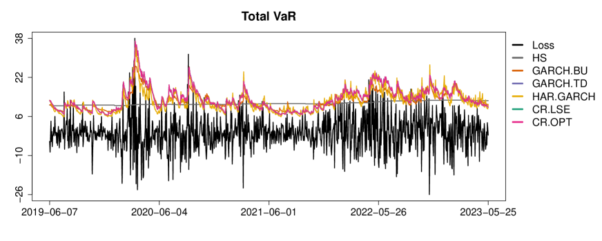
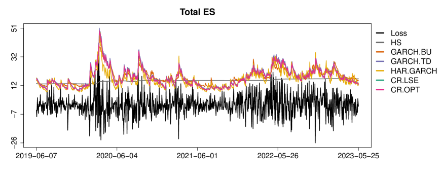
Figure S2: Time series plots of total VaR and total ES with confidence level $0.975$ estimated by the $6$ models. The black lines represent the time series of the total loss of the portfolio.

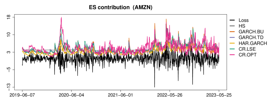
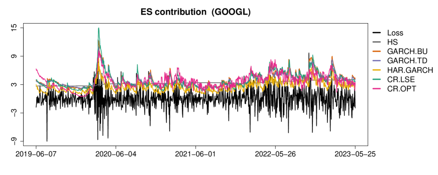
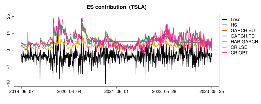
Figure S3: Time series plots of ES contributions with confidence level $0.975$ estimated by the $6$ models. The black lines represent the time series of the corresponding marginal losses.

S2.4 Backtests in the one-step approach

Due to multi-objective elicitability of ES contributions, we also conduct two-sided and “one and a half-sided” Wald-tests for tuple of ES contributions and each of them in combination with total VaR; see Section 5 of Fissler and Hoga (2023) for details of these tests. In this one-step approach the major difference from the two-step approach is that the null hypothesis includes equality in the accuracy of total VaRs for two competing forecasts . We report p-values of these tests in Table S5.

Table S5: Results of the Wald-tests to compare the forecast accuracy of ES contributions with CR.OPT as the benchmark model.

	p-valuea					p-valuea
H0	$=$ CR.OPT	$\leq$ CR.OPT	$\geq$ CR.OPT		H0	$=$ CR.OPT	$\leq$ CR.OPT	$\geq$ CR.OPT
(1) Tuple of ES contributions					(2) ES contribution (AMZN)
HS	0.007	0.012	0.004		HS	0.010	0.012	0.006
GARCH.BU	0.126	0.368	0.084		GARCH.BU	0.466	0.368	0.342
GARCH.TD	0.315	0.320	0.222		GARCH.TD	0.288	0.320	0.201
HAR.GARCH	0.316	0.929	0.223		HAR.GARCH	0.830	0.685	0.929
CR.LSE	0.735	1.000	0.584		CR.LSE	0.478	1.000	0.351
CR.OPT	—-	—-	—-		CR.OPT	—-	—-	—-
(3) ES contribution (GOOGL)					(4) ES contribution (TSLA)
HS	0.019	0.012	0.012		HS	0.011	0.012	0.007
GARCH.BU	0.453	0.368	0.330		GARCH.BU	0.098	0.368	0.065
GARCH.TD	0.406	0.292	0.320		GARCH.TD	0.359	0.320	0.255
HAR.GARCH	0.656	0.929	0.507		HAR.GARCH	0.328	0.929	0.231
CR.LSE	0.742	0.591	1.000		CR.LSE	0.788	1.000	0.639
CR.OPT	—-	—-	—-		CR.OPT	—-	—-	—-

• ^aThe p-values are calculated based on the three different null hypotheses with all of them including the equality of the accuracy of forecasted total VaRs, where “$=$ CR.OPT” means that the model is equally accurate as CR.OPT, and “$\leq$ ($\geq$) CR.OPT” represents the hypothesis that the model is less (more) accurate than CR.OPT.

Due to joint identifiability of total ES (see Section 2.1 of  Nolde and Ziegel, 2017) and $j$th ES contribution for $j=1,\dots,d$ (see Proposition 2) in combination with total VaR, we also conduct Wald-tests for these risk quantities in the one-step approach. Namely, for total ES, we consider the two-sided Wald-test for the null hypothesis:

$$H_{0}^{=}:\mathbb{E}\left[\bar{\operatorname{V}}_{T}^{\text{VaR}}\right]=0\quad\text{and}\quad\mathbb{E}\left[\bar{\operatorname{V}}_{T}^{\text{ES}}\right]=0,$$

and the “one and a half-sided” Wald-test for each of the null hypotheses:

$$H_{0}^{\leq_{\text{lex}}} :\mathbb{E}\left[\bar{\operatorname{V}}_{T}^{\text{VaR}}\right]=0\quad\text{and}\quad\mathbb{E}\left[\bar{\operatorname{V}}_{T}^{\text{ES}}\right]\leq 0,$$

$$H_{0}^{\geq_{\text{lex}}} :\mathbb{E}\left[\bar{\operatorname{V}}_{T}^{\text{VaR}}\right]=0\quad\text{and}\quad\mathbb{E}\left[\bar{\operatorname{V}}_{T}^{\text{ES}}\right]\geq 0,$$

based on Section 5 of Fissler and Hoga (2023) as considered in the above comparative backtests. For the $j$th ES contribution for $j\in\{1,\dots,d\}$, we replace $\bar{\operatorname{V}}_{T}^{\text{ES}}=(1/T)\sum_{t=1}^{T}\operatorname{V}_{t}^{\text{ES}}$ above with $\bar{\operatorname{V}}_{j,T}^{\text{ESC}}=(1/T)\sum_{t=1}^{T}\operatorname{V}_{j,t}^{\text{ESC}}$. We consider these null hypotheses since over- and under-estimations of ES contributions can be judged when the corresponding total VaR is calibrated; see Section 2.3. We summarize p-values of these tests in Table S6.

Table S6: Results of the Wald-tests to verify forecast accuracy of total ES and ES contributions.

	p-valuea					p-valuea
H0	$=$ True	$\leq$ True	$\geq$ True		H0	$=$ True	$\leq$ True	$\geq$ True
(1) Total ES					(2) ES contribution (AMZN)
HS	0.000	0.000	0.000		HS	0.000	0.000	0.000
GARCH.BU	0.014	0.009	0.034		GARCH.BU	0.052	0.034	0.034
GARCH.TD	0.061	0.040	0.204		GARCH.TD	0.266	0.185	0.204
HAR.GARCH	0.175	0.118	0.118		HAR.GARCH	0.016	0.118	0.010
CR.LSE	0.174	0.118	0.204		CR.LSE	0.263	0.183	0.204
CR.OPT	0.174	0.118	0.204		CR.OPT	0.232	0.159	0.204
(3) ES contribution (GOOGL)					(4) ES contribution (TSLA)
HS	0.000	0.000	0.000		HS	0.000	0.000	0.000
GARCH.BU	0.052	0.034	0.034		GARCH.BU	0.018	0.011	0.034
GARCH.TD	0.245	0.169	0.204		GARCH.TD	0.232	0.160	0.204
HAR.GARCH	0.003	0.118	0.002		HAR.GARCH	0.003	0.118	0.002
CR.LSE	0.253	0.175	0.204		CR.LSE	0.274	0.191	0.204
CR.OPT	0.291	0.204	0.203		CR.OPT	0.251	0.173	0.204

• ^aThe p-values are calculated based on the three different null hypotheses with all of them including the preciseness of forecasted total VaRs, where “$=$ True” means that the forecast is precise, “$\leq$ True” represents the hypothesis that the forecast is under-estimated, and “$\geq$ True” stands for the case when the forecast is over-estimated.

References

- Aitchison (1982) Aitchison, J. (1982). The statistical analysis of compositional data. Journal of the Royal Statistical Society: Series B (Methodological) 44(2), 139–160.
- Aitchison and J. Egozcue (2005) Aitchison, J. and J. J. Egozcue (2005). Compositional data analysis: where are we and where should we be heading? Mathematical Geology 37, 829–850.
- Andrews (1991) Andrews, D. W. (1991). Heteroskedasticity and autocorrelation consistent covariance matrix. Econometrica 59(3), 817–858.
- BCBS (2013) BCBS (2013). Consultative document October 2013. fundamental review of the trading book: A revised market risk framework. Basel Committee on Banking Supervision. Basel: Bank for International Settlements. BIS online publication. No. bcbs265.
- BCBS (2016) BCBS (2016). Minimum capital requirements for market risk. January 2016. Basel Committee on Banking Supervision. Basel: Bank for International Settlements. BIS online publication. No. d352.
- BCBS (2019) BCBS (2019). Minimum capital requirements for market risk. February 2019. Basel Committee on Banking Supervision. Basel: Bank for International Settlements. BIS online publication. No. d457.
- Bielecki et al. (2020) Bielecki, T. R., I. Cialenco, M. Pitera, and T. Schmidt (2020). Fair estimation of capital risk allocation. Statistics & Risk Modeling 37(1-2), 1–24.
- Boonen et al. (2019) Boonen, T. J., M. Guillen, and M. Santolino (2019). Forecasting compositional risk allocations. Insurance: Mathematics and Economics 84, 79–86.
- Chen et al. (2019) Chen, C. W., H. Than-Thi, M. K. So, and S. Sriboonchitta (2019). Quantile forecasting based on a bivariate hysteretic autoregressive model with garch errors and time-varying correlations. Applied Stochastic Models in Business and Industry 35(6), 1301–1321.
- Demarta and McNeil (2005) Demarta, S. and A. J. McNeil (2005). The t copula and related copulas. International statistical review 73(1), 111–129.
- Denault (2001) Denault, M. (2001). Coherent allocation of risk capital. Journal of Risk 4(1), 1–34.
- Dhaene et al. (2012) Dhaene, J., A. Tsanakas, E. A. Valdez, and S. Vanduffel (2012). Optimal capital allocation principles. Journal of Risk and Insurance 79(1), 1–28.
- Diebold and Mariano (1995) Diebold, F. X. and R. S. Mariano (1995). Comparing predictive accuracy. Journal of Business & Economic Statistics 13(3), 134–144.
- Dimitriadis and Hoga (2023) Dimitriadis, T. and Y. Hoga (2023). Dynamic covar modeling. arXiv preprint, 2206.14275.
- Egozcue et al. (2003) Egozcue, J. J., V. Pawlowsky-Glahn, G. Mateu-Figueras, and C. Barcelo-Vidal (2003). Isometric logratio transformations for compositional data analysis. Mathematical Geology 35(3), 279–300.
- Ehm et al. (2016) Ehm, W., T. Gneiting, A. Jordan, and F. Krüger (2016). Of quantiles and expectiles: consistent scoring functions, choquet representations and forecast rankings. Journal of the Royal Statistical Society Series B: Statistical Methodology 78(3), 505–562.
- Emmer et al. (2015) Emmer, S., M. Kratz, and D. Tasche (2015). What is the best risk measure in practice? a comparison of standard measures. Journal of Risk 18(2), 31–60.
- Fernández and Steel (1998) Fernández, C. and M. F. Steel (1998). On bayesian modeling of fat tails and skewness. Journal of the American Statistical Association 93(441), 359–371.
- Fissler and Hoga (2023) Fissler, T. and Y. Hoga (2023). Backtesting systemic risk forecasts using multi-objective elicitability. Journal of Business & Economic Statistics, 1–14.
- Fissler and Ziegel (2016) Fissler, T. and J. F. Ziegel (2016, Aug). Higher order elicitability and osband’s principle. The Annals of Statistics 44(4), 1680–1707.
- Fissler and Ziegel (2019) Fissler, T. and J. F. Ziegel (2019). Order-sensitivity and equivariance of scoring functions. Electronic Journal of Statistics 13, 1166–1211.
- Fissler et al. (2016) Fissler, T., J. F. Ziegel, and T. Gneiting (2016, January). Expected shortfall is jointly elicitable with value at risk-implications for backtesting. Risk Magazine, 58–61.
- Gribkova et al. (2023) Gribkova, N., J. Su, and R. Zitikis (2023). Estimating the var-induced euler allocation rule. ASTIN Bulletin: The Journal of the IAA 53(3), 619–635.
- Hofert et al. (2023) Hofert, M., I. Kojadinovic, M. Maechler, and J. Yan (2023). copula: Multivariate Dependence with Copulas. R package version 1.1-2.
- Huang et al. (2009) Huang, J.-J., K.-J. Lee, H. Liang, and W.-F. Lin (2009). Estimating value at risk of portfolio by conditional copula-garch method. Insurance: Mathematics and Economics 45(3), 315–324.
- Jondeau and Rockinger (2006) Jondeau, E. and M. Rockinger (2006). The copula-garch model of conditional dependencies: An international stock market application. Journal of International Money and Finance 25(5), 827–853.
- Kalkbrener (2005) Kalkbrener, M. (2005). An axiomatic approach to capital allocation. Mathematical Finance 15(3), 425–437.
- Koike and Hofert (2021) Koike, T. and M. Hofert (2021). Modality for scenario analysis and maximum likelihood allocation. Insurance: Mathematics and Economics 97, 24–43.
- Koike et al. (2022) Koike, T., Y. Saporito, and R. Targino (2022). Avoiding zero probability events when computing value at risk contributions. Insurance: Mathematics and Economics 106, 173–192.
- Maume-Deschamps et al. (2016) Maume-Deschamps, V., D. Rullière, and K. Said (2016). On a capital allocation by minimization of some risk indicators. European Actuarial Journal 6(1), 177–196.
- McNeil et al. (2015) McNeil, A. J., R. Frey, and P. Embrechts (2015). Quantitative risk management: Concepts, techniques and tools. Princeton: Princeton University Press.
- Newey and West (1987) Newey, W. K. and K. D. West (1987). A simple, positive semi-definite, heteroskedasticity and autocorrelation consistent covariance matrix. Econometrica 55(3), 703.
- Nolde and Ziegel (2017) Nolde, N. and J. F. Ziegel (2017). Elicitability and backtesting: Perspectives for banking regulation. The annals of Applied Statistics 11(4), 1833–1874.
- Patton (2020) Patton, A. J. (2020). Comparing possibly misspecified forecasts. Journal of Business & Economic Statistics 38(4), 796–809.
- Patton et al. (2019) Patton, A. J., J. F. Ziegel, and R. Chen (2019). Dynamic semiparametric models for expected shortfall (and value-at-risk). Journal of Econometrics 211(2), 388–413.
- Pawlowsky-Glahn and Buccianti (2011) Pawlowsky-Glahn, V. and A. Buccianti (2011). Compositional data analysis. Wiley Online Library.
- R Core Team (2023) R Core Team (2023). R: A Language and Environment for Statistical Computing. Vienna, Austria: R Foundation for Statistical Computing.
- Tasche (1999) Tasche, D. (1999). Risk contributions and performance measurement. Working Paper, Techische Universität München.
- Tasche (2008) Tasche, D. (2008). Capital allocation to business units and sub-portfolios: the euler principle. In A. Resti (Ed.), Pillar II in the New Basel Accord: The Challenge of Economic Capital, pp. 423–453. Risk Books: London.
- Taylor (2019) Taylor, J. W. (2019). Forecasting value at risk and expected shortfall using a semiparametric approach based on the asymmetric laplace distribution. Journal of Business & Economic Statistics 37(1), 121–133.
- Taylor (2022) Taylor, J. W. (2022). Forecasting value at risk and expected shortfall using a model with a dynamic omega ratio. Journal of Banking & Finance 140, 106519.
- Tse and Tsui (2002) Tse, Y. and A. Tsui (2002). A Multivariate Generalized Autoregressive Conditional Heteroscedasticity Model With Time-Varying Correlations. Journal of Business & Economic Statistics 20(3), 351–362.
- Wuertz et al. (2022) Wuertz, D., Y. Chalabi, T. Setz, and M. Maechler (2022). fGarch: Rmetrics - Autoregressive Conditional Heteroskedastic Modelling. R package version 4022.89.
- Ziegel et al. (2020) Ziegel, J. F., F. Krüger, A. Jordan, and F. Fasciati (2020). Robust forecast evaluation of expected shortfall. Journal of Financial Econometrics 18(1), 95–120.