Evolutionary dynamics of any multiplayer game on regular graphs

Abstract

Multiplayer games on graphs are at the heart of theoretical descriptions of key evolutionary processes that govern vital social and natural systems. However, a comprehensive theoretical framework for solving multiplayer games with an arbitrary number of strategies on graphs is still missing. Here, we solve this by drawing an analogy with the Ball-and-Box problem, based on which we show that the local configuration of multiplayer games on graphs is equivalent to distributing $k$ identical co-players among $n$ distinct strategies. We use this to derive the replicator equation for any $n$-strategy multiplayer game under weak selection, which can be solved in polynomial time. As an example, we revisit the second-order free-riding problem, where costly punishment cannot truly resolve social dilemmas in a well-mixed population. Yet, in structured populations, we derive an accurate threshold for the punishment strength, beyond which punishment can either lead to the extinction of defection or transform the system into a rock-paper-scissors-like cycle. The analytical solution also qualitatively agrees with the phase diagrams that were previously obtained for non-marginal selection strengths. Our framework thus allows an exploration of any multi-strategy multiplayer game on regular graphs.

Multi-strategy evolutionary dynamics in nature often lead to diverse and complex phenomena, such as cyclic dominance that is captured by the well-known rock-paper-scissors game [1]. Experimental evidence from diverse contexts, ranging from the three-morph mating system of the side-blotched lizard [2] and Escherichia coli populations [3], to human economic behaviors [4], demonstrates the occurrence of the rock-paper-scissors cycle in various real-world scenarios. Theoretical models of the rock-paper-scissors cycle have been explored in both two-player [5] and multiplayer game frameworks [6], contributing to an understanding of its underlying properties — as a consequence of strategy diversity, the intransitive interaction may emerge spontaneously. This phenomenon can be illustrated when we extend the basic two-strategy model of the evolution of cooperation by adding additional strategies that punish defectors [7, 8] or reward cooperators [9, 10]. The additional strategies are necessary when considering more realistic models, which underlines the importance of a multi-strategy approach.

Previous research in evolutionary dynamics primarily focused on two-strategy systems, where the unconditional cooperator and defector strategies represent the fundamental conflict of individual and collective interests [11]. While cooperation can maximize mutual benefits, defection, despite offering higher personal payoff, reduces overall benefits to others. Consequently, defection often appears as the dominant strategy. An escape route from this dilemma could be a spatially structured population [12, 13], where individuals interact with fixed neighbors but still adopt the strategies of those with higher payoffs. This setting allows cooperation to form clusters, utilizing the advantage of collective payoffs thus resisting the invasion of defection, a concept known as spatial reciprocity [14]. It is recognized that no simple closed-form solution exists for general evolutionary dynamics in structured populations, unless by chance P=NP, Polynomial time equals to Nondeterministic Polynomial time [15]. However, in the weak selection limit, where the influence of the game on strategy updates is marginal, analytical solutions have been obtained from infinite [16] to finite populations [17], and from regular [18, 19] to arbitrary graphs [20, 21, 22, 23]. This line of research has led to the development of evolutionary graph theory [14].

In evolutionary graph theory, a widely used mathematical technique is the pair approximation [24, 25, 26, 27, 28]. This method applies to infinite populations on regular graphs and has revealed the well-known ‘$b/c>k$’ rule, which states that evolution favors cooperation when the benefit-to-cost ratio exceeds the number of neighbors [29]. Pair approximation is also capable of analyzing more complex models, including unequal interaction and dispersal graphs [30], asymmetric networks [31], and stochastic games [32], predicting simulation outcomes with high accuracy. Notably, pair approximation has been applied to multi-strategy two-player games [33], leading to the replicator equations for arbitrary $n$-strategy two-player games on a regular graph, as an important extension of the traditional replicator equations used in well-mixed populations [34].

Unlike two-player games, multiplayer games exhibit much greater complexity, primarily due to their potentially nonlinear payoff functions [35]. In a structured population, multiplayer games require each individual to organize a game within their neighbors and themselves, which implies that individuals participate in games organized by both themselves and their neighbors, thereby interacting with second-order neighbors. Such interactions lead to higher-order interactions [36, 37], which cannot be simply reduced to a superposition of pairwise interactions. The complexity of multiplayer games can also be illustrated from the perspective of structure coefficients on graphs: a two-strategy two-player game needs only one structure coefficient [38], a multi-strategy two-player game requires three [39, 40], but a two-strategy ($k+1$)-player game needs as many as $k$ structure coefficients [41, 42]. Even so, in the absence of triangle motifs, two-strategy multiplayer games can still be theoretically analyzed using pair approximation [43, 44], whose results are consistent with predictions obtained by other more precise methods [45, 46].

With two-strategy two-player [29], multi-strategy two-player [33], and two-strategy multiplayer games [44] all thoroughly studied, the analytical solution for multi-strategy multiplayer games on graphs remains unexplored. The range of potential models for multiplayer games with more than two strategies is vast, drawing from co-evolutionary strategies such as punishment [47, 48, 8, 49], reward [9, 50, 51], and the loner strategy [52, 4]. Multi-strategy systems in multiplayer games have unique characteristics that multi-strategy two-player games do not capture: the payoff function can be nonlinear. For example, in pool punishment, the payoff structure depends solely on whether there is at least one punishing player among the $k+1$ players. This uniqueness reinforces the significance of studying multi-strategy multiplayer games.

However, previous research on these games on graphs has largely been limited to numerical simulations, which do not allow for the exploration of the complete parameter space. In the absence of mathematical tools for evolutionary graph theory in multi-strategy multiplayer games, recent studies have attempted to bypass this challenge by incorporating the third strategy within the existing two strategies. For instance, punishing or rewarding behaviors have been added to the existing cooperation strategy in the traditional two-strategy system [53, 54]. This approach allows for the examination of additional mechanisms like punishment and reward within the two-strategy system’s framework. Yet, these alternative attempts still could not capture further rich dynamics, such as cyclic dominance, which is only possible in systems with at least three strategies.

In this Article, we provide an analytical framework that addresses the gaps in multi-strategy multiplayer games in the realm of evolutionary graph theory. We demonstrate that for a given multi-strategy multiplayer game, the co-player configuration of a focal individual is equivalent to the well-known Ball-and-Box problem, distributing $k$ identical co-players into $n$ distinct strategies. Building on this analogy, we develop a bottom-up approach for calculating the statistical mean payoff of individuals on regular graphs, deriving replicator equations on regular graphs in the weak selection limit and the absence of triangle motifs. Our results include two commonly used update rules, namely pairwise comparison (PC) [55] and death-birth (DB) [29], applicable to arbitrary multiplayer games with any multi-strategy space in structured populations, where each individual has the same number of neighbors. Using the punishment mechanism [7, 56, 57] in the context of the tragedy of the commons [58] as an example, we explore the well-known second-order free-riding problem analytically, obtaining an accurate threshold of punishment strength necessary to resolve the social dilemma in structured populations. Additionally, our theoretical solutions can qualitatively reproduce the phase diagrams observed in previous numerical simulation studies under non-marginal selection strength.

Results

Model overview

We consider an infinite population on a regular graph, where each individual has $k$ neighbors. An individual can adopt one of $n$ strategies, labeled by the numbers $1,2,\dots,n$. On a regular graph, the number of co-players in every multiplayer game is equivalent to the number of neighbors. For a given individual, suppose that there are $k_{1}$ co-players employing strategy $1$, $k_{2}$ co-players employing strategy $2$, and so on, up to $k_{n}$ co-players employing strategy $n$. In this context, the co-player configuration of an individual can be represented by $\mathbf{k}=(k_{1},k_{2},\dots,k_{n})$, which satisfies the condition $\sum_{l=1}^{n}k_{l}=k$. As illustrated in Fig. 1a, counting the number of possible configurations of $\mathbf{k}$ is analogous to the classic Ball-and-Box problem, distributing $k$ identical balls (i.e., co-players) into $n$ distinct boxes (i.e., strategies), allowing for the possibility of empty boxes (e.g., $k_{1}=0$). Hence, there are $\mathbb{C}(k+n-1,k)=(k+n-1)!/[(n-1)!k!]$ possible configurations of co-player strategy configurations $\mathbf{k}$.

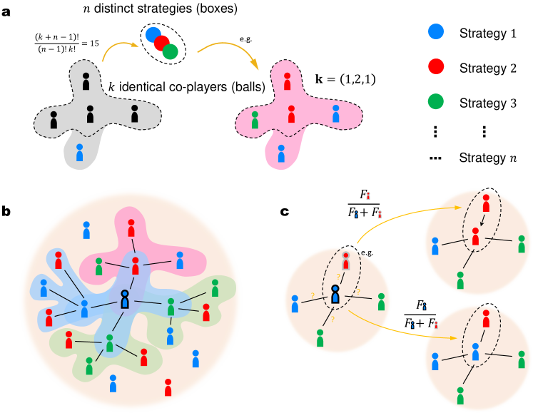
Figure 1: The Ball-and-Box problem, payoff calculation, and strategy updates. a, To determine a co-player configuration, we distribute $k$ identical co-players (balls) into $n$ distinct strategies (boxes), corresponding to the classic Ball-and-Box problem. For instance, with $k=4$ and $n=3$, there are $15$ possible co-player configurations. b, An individual accumulates payoffs from $1+k$ multiplayer games, organized by itself and its $k$ neighbors. Each multiplayer game involves $k+1$ players, including the organizer and its neighbors. c, Strategy updates in an individual are governed by the pairwise comparison rule. A random neighbor is selected, and the focal individual either adopts the neighbor’s strategy or maintains its original strategy, based on a probability proportional to the fitness (transformed from payoffs) in the pair.

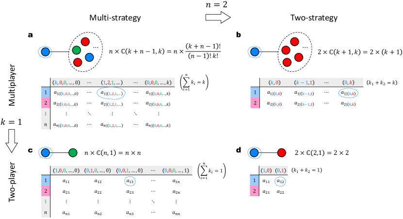
Figure E1: Generalized payoff matrix for multi-strategy multiplayer games, reducible to two-strategy or two-player formats. a, Payoff matrix for $n$-strategy ($k+1$)-player games: with $n$ strategies and $k$ co-players, the matrix size is $n\times\mathbb{C}(k+n-1,k)$. b, Payoff matrix for $2$-strategy ($k+1$)-player games [44]: with $n=2$ strategies and $k$ co-players, the matrix size is $2\times\mathbb{C}(k+1,k)$. c, Payoff matrix for $n$-strategy $2$-player games [33]: with $n$ strategies and $k=1$ co-players, the matrix size is $n\times\mathbb{C}(n,1)$. d, Payoff matrix for $2$-strategy $2$-player games [29]: with $n=2$ strategies and $k=1$ co-players, the matrix size is $2\times\mathbb{C}(2,1)$.

Interaction occurs between an individual and its $k$ co-players. In a multiplayer game involving the focal individual and $k$ co-players, the payoff is uniquely determined by the strategy of the focal individual and the strategy configuration of the co-players. For a focal individual employing strategy $i$ with the co-player configuration $\mathbf{k}$, its payoff is denoted by $a_{i|\mathbf{k}}$. It can be observed that the ‘generalized payoff matrix’ comprises $n\times\mathbb{C}(k+n-1,k)$ elements represented by $a_{i|\mathbf{k}}$ through all possible focal strategies $i=1,2,\dots,n$ and co-player strategy configurations $\mathbf{k}$. For two-strategy two-player games ($n=2$, $k=1$), the number of elements in the payoff matrix reduces to $2\times\mathbb{C}(2,1)=4$; for multi-strategy two-player games ($k=1$), it reduces to $n\times\mathbb{C}(n,1)=n^{2}$; for two-strategy multiplayer games ($n=2$), it reduces to $2\times\mathbb{C}(k+1,k)=2(k+1)$ (Fig. E1).

The accumulated payoff of a focal individual is collected from the $1+k$ games organized by itself and its neighbors, as depicted in Fig. 1b. Upon obtaining the accumulated payoffs $\pi$, we convert them into fitness, denoted as $F=\exp{(\delta\pi)}$ [21, 46, 59, 60]. Strategies that yield higher fitness are more likely to reproduce. Here, $\delta\to 0^{+}$ represents a weak selection strength. The rationale behind weak selection is that, in reality, many factors other than the investigated game influence the probability of reproduction [29].

There are various commonly used strategy update rules. For simplicity, we focus on the pairwise comparison (PC) rule [55] in the main text (another well-known rule, the death-birth, is discussed in the Methods and Supplementary Information). During each elementary step, an individual $A$ and one of its neighbors $B$ are randomly selected from the population. Their payoffs are computed as $\pi_{A}$ and $\pi_{B}$ and then transformed into fitness values $F_{A}$ and $F_{B}$. Individual $A$ adopts the strategy of individual $B$ with a probability proportional to their fitness in the pair,

$$W=\frac{F_{B}}{F_{A}+F_{B}}=\frac{1}{1+\exp{[-\delta(\pi_{B}-\pi_{A})]}}.$$ (1)

Or, individual $A$ keeps its own strategy with the remaining probability $F_{A}/(F_{A}+F_{B})$. Eq. (1) indicates that individual $A$ has a marginal tendency to either maintain its own strategy or adopt the one of individual $B$, depending on who has higher fitness. The evolution of strategies under the PC update process is illustrated in Fig. 1c.

The statistical mean payoff

To formally analyze the evolutionary dynamics, we construct the system as described in Supplementary section S1.1. There are two key concepts, the frequency of $i$-players (i.e., individuals employing strategy $i$), denoted as $x_{i}$, where $\sum_{i=1}^{n}x_{i}=1$, and the probability of an $i$-player being adjacent to a $j$-player, denoted by $q_{i|j}$, with $\sum_{j=1}^{n}q_{j|i}=1$. By separating different time scales, we find that $q_{i|j}=x_{i}(k-2)/(k-1)+\theta_{ij}/(k-1)$, where $\theta_{ij}=1$ if $i=j$ and $\theta_{ij}=0$ otherwise (Supplementary section B.1). In other words, the value of $q_{i|j}$ can be determined by the value of $x_{i}$.

To express necessary computations, we introduce a variation of $\mathbf{k}$, denoted as $\mathbf{k}_{+l}=(k_{1},k_{2},\dots,k_{l}+1,\dots,k_{n})$, where $\sum_{l=1}^{n}k_{l}=k-1$. This represents a co-player configuration in which there is at least one $l$-player. Among the remaining $k-1$ co-players, the numbers of players adopting strategies $1,2,\dots,n$ are $k_{1},k_{2},\dots,k_{n}$, respectively.

At the single game level, we use $\langle a_{X|\mathbf{k}}\rangle_{Y}$ to denote the statistical mean payoff for an $X$-player in a single game, defined by Eq. (12) in the Methods, calculated over the possible co-player configurations $\mathbf{k}$, where the $k$ members in $\mathbf{k}$ are neighbors of a $Y$-player. Similarly, the notation $\langle a_{X|\mathbf{k}_{+l}}\rangle_{Y}$ differs in that it is over $k-1$ unknown members in the possible co-player configurations $\mathbf{k}_{+l}$, with one known $l$-player.

At the accumulated payoff level, we use the notation $\langle\pi_{X}^{\mathbf{k}}\rangle$ to represent the expected payoff of an $X$-player accumulated from the $1+k$ games organized by the player and its neighbors, across all possible neighbor configurations $\mathbf{k}$ of the $X$-player, defined by Eq. (10) in the Methods. Similarly, $\langle\pi_{X}^{\mathbf{k}_{+i}}\rangle$ denotes the expected accumulated payoff, as defined by Eq. (11) in the Methods, computed over the configurations where the remaining $k-1$ neighbors are unknown besides one known $i$-player.

Through bottom-up calculations from the microscopic level (Methods), we establish the following relationship between the accumulated and single-game statistical mean payoffs. For $i$-players, the relation is given by

$$\langle\pi_{i}^{\mathbf{k}}\rangle=\langle a_{i|\mathbf{k}}\rangle_{i}+k\sum_{l=1}^{n}q_{l|i}\langle a_{i|\mathbf{k}^{\prime}_{+l}}\rangle_{l}.$$ (2)

Intuitively, the expected accumulated payoff of $i$-players, $\langle\pi_{i}^{\mathbf{k}}\rangle$, is composed by the statistical mean payoff from the game they organize, $\langle a_{i|\mathbf{k}}\rangle_{i}$, and the games organized by their $k$ neighbors, $k\sum_{l=1}^{n}q_{l|i}\langle a_{i|\mathbf{k}^{\prime}_{+l}}\rangle_{l}$. Here, the different notation $\mathbf{k}^{\prime}=(k^{\prime}_{1},k^{\prime}_{2},\dots,k^{\prime}_{n})$ from $\mathbf{k}$ is only to clarify the priority in the summation. It is equivalent to $\mathbf{k}$ when they are independent of each other, as in Eq. (2).

A further concept is the expected accumulated payoff of a $j$-player who has at least one $i$-player as a neighbor, which is related to the statistical mean payoff in single games as follows:

$$\langle\pi_{j}^{\mathbf{k}_{+i}}\rangle=\langle a_{j|\mathbf{k}_{+i}}\rangle_{j}+\langle a_{j|\mathbf{k}^{\prime}_{+i}}\rangle_{i}+(k-1)\sum_{l=1}^{n}q_{l|j}\langle a_{j|\mathbf{k}^{\prime}_{+l}}\rangle_{l}.$$ (3)

Here, $\langle a_{j|\mathbf{k}_{+i}}\rangle_{j}$ is the mean payoff from the game organized by the $j$-player itself, $\langle a_{j|\mathbf{k}^{\prime}_{+i}}\rangle_{i}$ is the mean payoff from the game organized by the fixed $i$-player neighbor, and $(k-1)\sum_{l=1}^{n}q_{l|j}\langle a_{j|\mathbf{k}^{\prime}_{+l}}\rangle_{l}$ is the mean payoff from the games organized by the remaining $k-1$ neighbors of the $j$-player.

General replicator equations

The evolution of frequencies $x_{1},x_{2},\dots,x_{n}$ can be deduced through the microscopic strategy update process. Specifically, in an infinitely population $N\to\infty$, a single unit of time comprises $N$ elementary steps, ensuring that each individual has an opportunity to update their strategy. During each elementary step, the frequency of $i$-players increases by $1/N$ when a focal $j$-player (where $j\neq i$) is chosen to update its strategy and is replaced by an $i$-player. Similarly, the frequency of $i$-players decreases by $1/N$ when a focal $i$-player is selected to update its strategy and the player who takes the position is not an $i$-player. Based on this perception, we derive a simple form of the replicator equations for $i=1,2,\dots,n$ in the weak selection limit (Supplementary Information section S2):

$$\dot{x}_{i}=\frac{\delta}{2}x_{i}\left(\langle\pi_{i}^{\mathbf{k}}\rangle-\sum_{j=1}^{n}q_{j|i}\langle\pi_{j}^{\mathbf{k}_{+i}}\rangle\right).$$ (4)

We find that Eq. (4) offers an intuitive understanding and is comparable to the previous result derived from the identity-by-descent (IBD) idea, if we introduce the following two concepts: (1) $\pi_{i}^{(0)}=\langle\pi_{i}^{\mathbf{k}}\rangle$, the expected accumulated payoff of the $i$-player (zero steps away on the graph), and (2) $\pi_{i}^{(1)}=\sum_{j=1}^{n}q_{j|i}\langle\pi_{j}^{\mathbf{k}_{+i}}\rangle$, the expected accumulated payoff of the $i$-player’s neighbors (one step away on the graph). These concepts suggest that $\dot{x}_{i}\sim x_{i}(\pi_{i}^{(0)}-\pi_{i}^{(1)})$. Under pairwise comparison, the reproduction rate of $i$-players is dependent on how their accumulated payoff exceeds that of their neighbors. In essence, the evolution of $x_{i}$ a competition between an individual and its first-order neighbors, which aligns with the results obtained from the IBD idea in two-strategy systems [18, 20, 32]. We further extend it to $n$-strategy systems, albeit under deterministic dynamics. We also show that the death-birth rule is essentially the competition between an individual and its second-order neighbors for $n$-strategy systems (Methods).

Applying Eqs. (2) and (3) to Eq. (4), we can transform the expected accumulated payoff in the replicator equations into the statistical mean payoff of single games, as shown in Eq. (13) in the Methods, which is of the simplest irreducible complexity for computation given the payoff structure $a_{i|\mathbf{k}}$. In particular, we only need to calculate two types of quantities, $\langle a_{i|\mathbf{k}_{+j}}\rangle_{i}$ and $\langle a_{i|\mathbf{k}_{+j}}\rangle_{j}$ for $i,j=1,2,\dots,n$, based on the given payoff structure $a_{i|\mathbf{k}}$. The diagonal elements of these quantities coincide, as demonstrated in Eqs. (14) and (15) in the Methods. Therefore, for any given payoff structure $a_{i|\mathbf{k}}$, there are only $(2n-1)n$ distinct quantities to calculate manually to determine the replicator equations. The computational complexity is $\mathrm{O}(n^{2})$, square of the number of strategies, which can be solved within polynomial time. We also show that the computational complexity under the death-birth rule is $\mathrm{O}(n^{3})$, which can also be solved within polynomial time (Methods).

For specific payoff structures, the complexity of computation can be further reduced. A common example is linear systems. In such systems, the payoff function includes at most linear terms in $k_{1},k_{2},\dots,k_{n}$. This allows us to express the general payoff function in linear systems as $a_{i|\mathbf{k}}=\sum_{j=1}^{n}b_{ij}k_{j}+c_{i}$, where $b_{ij}$ represents the coefficient of the linear term and $c_{i}$ is the constant term, for $i,j=1,2,\dots,n$. Applying this special payoff structure to Eq. (13) in the Methods, we can obtain a simplified form of the replicator equation,

$$\dot{x}_{i}=\frac{\delta(k-2)}{2(k-1)}x_{i}\left((k+1)(\bar{\pi}_{i}-\bar{\pi})+3\sum_{j=1}^{n}x_{j}(b_{ii}-b_{ij}-b_{ji}-b_{jj})+6\sum_{j=1}^{n}\sum_{l=1}^{n}x_{j}x_{l}b_{jl}\right).$$ (5)

Here, $\bar{\pi}_{i}$ and $\bar{\pi}$ denote the mean payoff of $i$-players and all players in a well-mixed population, which can be directly calculated using the traditional replicator dynamics approach for well-mixed populations (Methods).

As a frequently studied example, the public goods game involves $n=2$ strategies within a linear payoff structure. Strategy 1, cooperation ($C$), pays a cost $c$ which is multiplied by a synergy factor $r$ and distributed among all $k+1$ players, while strategy 2, defection ($D$), pays nothing. The payoff structure can be expressed as $b_{11}=b_{21}=rc/(k+1)$, $b_{12}=b_{22}=0$, $c_{1}=rc/(k+1)-c$, $c_{2}=0$. Consequently, $\dot{x}_{i}\sim x_{i}(\bar{\pi}_{i}-\bar{\pi})$, indicating that evolution favors cooperation when $r>k+1$ (Supplementary Information section S3.1). Coincidentally, the public goods game exhibits an equivalence between well-mixed and structured populations under pairwise comparison, a phenomenon not necessarily observed under other update rules (see ref. [43]). This equivalence provides a unique opportunity: when introducing additional strategies into the public goods game, the distinct effects of these new strategies in structured populations can be isolated without interference from the existing two strategies, which have no impact in structured populations. For a general condition when pairwise comparison equates well-mixed and structured populations, we refer to the Supplementary Information section S3.1.3.

Next, we apply our framework to two specific examples—peer and pool punishment in public goods games—where the number of strategies increases to $n=3$.

Peer punishment in public goods games

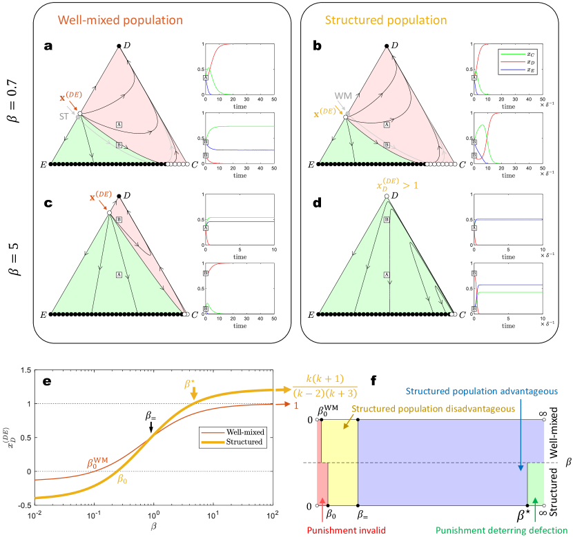
Figure 2: Peer punishment can resolve the social dilemma of public goods game in structured populations. a and b, The state space is bifurcated by $\mathbf{x}^{(DE)}$ and $\mathbf{x}_{\star}^{(CE)}$. The final state, either $D$ or $(C+E)_{\text{V}}$, is determined by the initial conditions. Under mild punishment ($\beta=0.7$), a structured population hinders cooperation by reducing the state space leading to the $(C+E)_{\text{V}}$ outcome. c and d, Conversely, with strong punishment ($\beta=5$), structured populations consistently result in the extinction of defection, thereby resolving the social dilemma in public goods games. In contrast, the state space in well-mixed populations remains divided into two distinct basins. e, As the punishment strength $\beta$ increases, $x_{D}^{(DE)}$ increases, expanding the initial space leading to the $(C+E)_{\text{V}}$ outcome. In well-mixed populations, $x_{D}^{(DE)}\to 1$ as $\beta\to\infty$, and the basin leading to defection cannot be completely eliminated. However, in structured populations, $x_{D}^{(DE)}\to k(k+1)/[(k-2)(k+3)]>1$ when $\beta>\beta^{\star}$, invariably resulting in the extinction of defection. f, The diagram of the different effects of punishment in well-mixed versus structured populations. Structured populations are advantageous in promoting cooperation under strong punishment but are less effective when the punishment is mild. Input parameters: $r=3$, $c=1$, $\alpha=0.7$, $k=4$.

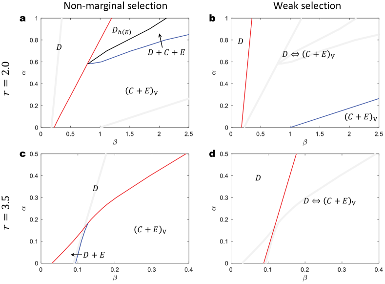
Figure 3: Phase diagrams of the system behavior with respect to punishing cost $\alpha$ and fine $\beta$ are qualitatively similar under non-marginal and weak selection strength. a and c (taken from Fig. 3 and 4 in ref. [49]), Numerical simulations under non-marginal selection ($\delta=2$). Here, the different phases are defined as follows: $D$—only $D$ exists; $D_{h(E)}$—only $D$ or $E$ exists based on certain probabilities; $D+C+E$—$D$, $C$, and $E$ coexist; $(C+E)_{\text{V}}$—$C$ and $E$ coexist like in the Voter model. b and d, The phase diagram created by analytical $\beta_{0}$ and $\beta^{\star}$ under weak selection ($\delta\to 0$), where $\beta_{0}$ divides the $D$ and $D\Leftrightarrow(C+E)_{\text{V}}$ phases, $\beta^{\star}$ separates the $D\Leftrightarrow(C+E)_{\text{V}}$ and $(C+E)_{\text{V}}$ phases. Specifically, in b, $\beta_{0}=3/17+(3/17)\alpha$ (red), $\beta^{\star}=1+(17/3)\alpha$ (blue); in d, $\beta_{0}=3/34+(3/17)\alpha$. The definition of the $D\Leftrightarrow(C+E)_{\text{V}}$ phase—the system finally evolves to either the $D$ phase or the $(C+E)_{\text{V}}$ phase, depending on initial conditions. Other parameters: $c=1$, $k=4$.

To apply our general results to specific models where $n>2$ to specific models, we begin with peer punishment in public goods games [61, 62]. The payoff structure in this model is also linear, which conveniently allows us to utilize Eq. (5).

There are $n=3$ strategies: $1=\text{Cooperation ($C$)}$, $2=\text{Defection ($D$)}$, and $3=\text{Peer punishment ($E$)}$. Besides the foundational 2-strategy in the public goods game, the third strategy, peer punishment, pays a cost $\alpha$ for punishing a co-player who defects. A defector, when punished, incurs a fine $\beta$. Thus, given $k_{2}$ defective co-players, a punishing player has $\alpha k_{2}$ paid, and given $k_{3}$ punishment co-players, a defector has $\beta k_{3}$ charged. Furthermore, it is assumed that punishing players also perform the cooperative behavior, investing $c$ to the common pool. This makes the strategy $C$ the second-order free-rider who exploits the effort in punishment of strategy $E$.

Analyzing both well-mixed and structured populations (Methods), we find that peer punishment introduces a bi-stable space of the system state, as seen in Fig. 2a, b. Even when $r<k+1$, the system can either evolve to a final state where strategies $E$ and $C$ coexist, or to a state dominated by strategy $D$, depending on the initial conditions. As the punishing fine $\beta$ increases, the basin of attraction for strategy $D$ diminishes. In a well-mixed population, strategy $D$ maintains a basin of attraction regardless of the punishment strength (Fig. 2c). This aligns with previous findings that peer punishment does not truly resolve social dilemmas in well-mixed populations [57]. However, in structured populations, we observe that the basin of attraction for strategy $D$ can be entirely eliminated if the punishing fine $\beta$ exceeds a critical threshold, $\beta>\beta^{\star}$, where

$$\beta^{\star}=\frac{k+1}{3}\left(-\frac{rc}{k+1}+c+k\alpha\right)-\alpha.$$ (6)

Consequently, in such scenarios, the system consistently converges to a coexistence of strategies $E$ and $C$ (Fig. 2d). The numerical observation from previous research suggests that peer punishment can effectively resolve social dilemmas in structured populations. Our analysis adds an analytical perspective to this conclusion.

The distinct roles of peer punishment in well-mixed and structured populations can be attributed to the fraction of defectors, $x_{D}^{(DE)}$, in an unstable edge equilibrium, $\mathbf{x}^{(DE)}=(0,x_{D}^{(DE)},1-x_{D}^{(DE)})$, as presented in Fig. 2e. When $x_{D}^{(DE)}>1$, this unstable equilibrium disappears, rendering the $D$-vertex equilibrium unstable. In a well-mixed population, $x_{D}^{(DE)}<1$ and $x_{D}^{(DE)}\to 1$ as $\beta\to\infty$, indicating that the described scenario is unattainable. However, in structured populations, $x_{D}^{(DE)}>1$ becomes feasible once $\beta>\beta^{\star}$. Additionally, peer punishment acts as a double-edged sword. When $x_{D}^{(DE)}<0$, the system invariably converges to the full defection state, signifying ineffective punishment. As the punishing fine $\beta$ increases, peer punishment first becomes effective in well-mixed populations when $\beta>\beta_{0}^{\text{WM}}$. Structured populations, in contrast, require a higher $\beta_{0}$ value for punishment to be effective. In particular, peer punishment is less advantageous in structured populations than in well-mixed populations when $\beta<\beta_{=}$ (Fig. 2a, b). However, structured populations gain an advantage when $\beta>\beta_{=}$, and can eventually lead to the extinction of defection at sufficient high $\beta>\beta^{\star}$ values. The comparison between well-mixed and structured populations in relation to the punishing fine is illustrated in Fig. 2f, and the expressions for key $\beta$ values are listed in Fig. E3.

The analytical results align qualitatively with the $\alpha$-$\beta$ phase diagram presented in previous research [49], as shown in Fig. 3. Although there are differences in detail between the results obtained from non-marginal selection through numerical simulations (Fig. 3a, c) and those derived under weak selection via analytical solutions (Fig. 3b, d), both approaches consistently predict unique behaviors in structured populations that are absent in well-mixed populations. For instance, both the non-marginal and weak selection strengths indicate the existence of a $(C+E)_{\text{V}}$ phase at low $\alpha$ and high $\beta$, where strategy $D$ becomes extinct and strategies $C$ and $E$ coexist, equivalent to the Voter model [63, 64]. Moreover, at moderate levels of $\alpha$ and $\beta$, we anticipate a $D\Leftrightarrow(C+E)_{\text{V}}$ phase under weak selection. In this phase, the system evolves towards either $D$ or $(C+E)_{\text{V}}$ based on the initial state, although strategy $C$ may eventually become extinct due to the continuous introduction of a small number of defectors [65]. A similar phase, named $D_{h(E)}$, is detected under non-marginal selection. The term ‘$h$’ denotes ‘homoclinic instability’, implying that strategy $E$ can overcome $D$ through a nucleation mechanism, particularly if a small colony of $E$ players survives after the extinction of cooperators. This likelihood increases with larger populations.

Pool punishment in public goods games

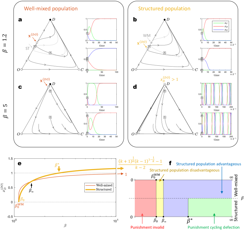
Figure 4: Pool punishment can resolve the social dilemma of public goods game in structured populations. a and b, In the three-strategy system space, the state consistently converges to full $D$. However, along the $DO$ edge, an unstable equilibrium point, $\mathbf{x}^{(DO)}$, creates a bi-stable space. In the $D$ versus $O$ dynamics, the final state, either $D$ or $O$, is determined by the initial conditions. Under mild punishment ($\beta=1.2$), a structured population tends to favor defection, reducing the basin leading to the $O$ outcome. c and d, Conversely, with strong punishment ($\beta=5$), structured populations result in the cyclic dominance of the three strategies, thereby preventing the full $D$ state in public goods games. In contrast, the state space in well-mixed populations remains two distinct basins on the $DO$ edge, preventing cyclic dominance. e, As the punishment strength $\beta$ increases, $x_{D}^{(DO)}$ increases, expanding the initial space leading to the $O$ outcome. In well-mixed populations, $x_{D}^{(DO)}\to 1$ as $\beta\to\infty$, and the basin leading to defection cannot be completely eliminated. However, in structured populations, $x_{D}^{(DO)}\to[(k+1)^{1/k}(k-1)^{1-1/k}-1]/(k-2)>1$ when $\beta>\beta^{\star}$, invariably resulting in the cyclic dominance of the three strategies. f, The diagram of the different effects of punishment in well-mixed versus structured populations. Structured populations are advantageous in promoting cooperation under strong punishment but are a bit less effective when the punishment is mild. Input parameters: $r=3$, $c=1$, $\alpha=0.7$, $k=4$.

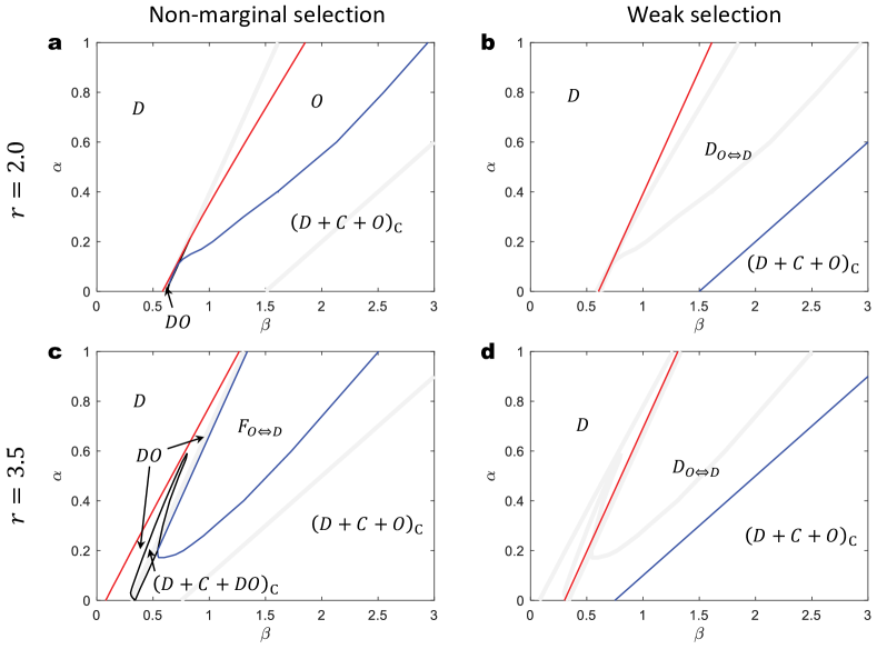
Figure 5: Phase diagrams of the system behavior with pool punishment are qualitatively similar under non-marginal and weak selection strength. a and c (taken from Fig. 5 and 10 in ref. [8]), Numerical simulations under non-marginal selection ($\delta=2$). The phases are defined as follows: $D$—only $D$ exists; $O$—only $O$ exists; $(D+C+O)_{\text{C}}$—cyclic dominance among $D$, $C$, and $O$; $F_{O\Leftrightarrow D}$—fixation of either $O$ or $D$; $DO$—$D$ and $O$ coexist; $(D+C+DO)_{\text{C}}$—cyclic dominance among $D$, $C$, and $DO$. b and d, The phase diagram is divided by analytical $\beta_{0}$ and $\beta^{\star}$ under weak selection ($\delta\to 0$). Here, $\beta_{0}$ divides the $D$ and $D_{O\Leftrightarrow D}$ phases, while $\beta^{\star}$ separates the $D_{O\Leftrightarrow D}$ and $(D+C+O)_{\text{C}}$ phases. Specifically, in b, $\beta_{0}=81/134+(135/134)\alpha$ (red), $\beta^{\star}=3/2+(5/2)\alpha$ (blue); in d, $\beta_{0}=81/268+(135/134)\alpha$, $\beta^{\star}=3/4+(5/2)\alpha$. The definition of the $D_{O\Leftrightarrow D}$ phase—the system finally evolves to full $D$ if cooperation is initially present, or to the fixation of either $O$ or $D$ in the absence of initial cooperators. Other parameters: $c=1$, $k=4$.

Another example is pool punishment in public goods games [8, 66]. From the perspective of computational complexity, pool punishment differs from peer punishment in its nonlinear payoff structure, which requires utilizing Eq. (13).

Similarly, there are $n=3$ strategies: $1=\text{Cooperation ($C$)}$, $2=\text{Defection ($D$)}$, and $3=\text{Pool punishment ($O$)}$. Again, based on the 2-strategy public goods game, the third strategy, pool punishment, contributes a cost $\alpha$ to the public pool for punishment. A defector is punished with a fine $\beta$ if the public pool for punishment has funds (i.e., there is at least one punisher among the co-players); if no punishers are present, the defector incurs no charge. Irrespective of the number of defecting co-players $0\leq k_{2}\leq k$, a punishing player pays $\alpha$. It is also assumed that those employing pool punishment engage in cooperative behavior, investing $c$ to the common pool, making the strategy $C$ a second-order free-rider.

Our analysis of both well-mixed and structured populations (Methods) reveals that pool punishment does not change the fact that the system cannot converge to a defection-free state when $r<k+1$, as demonstrated in Fig. 4a, b. However, along the $DO$ edge (i.e., without the presence of strategy $C$), the system can evolve to a final state of either full $D$ or full $O$, depending on the initial conditions. As the punishing fine $\beta$ increases, the attraction basin for strategy $D$ shrinks. In well-mixed populations, strategy $D$ retains an attraction basin regardless of the punishment strength (Fig. 4c). This is consistent with previous findings that pool punishment does not effectively resolve social dilemmas in well-mixed populations [57]. However, in structured populations, the attraction basin for strategy $D$ can be completely eliminated if the punishing fine $\beta$ exceeds a critical threshold, $\beta>\beta^{\star}$, where

$$\beta^{\star}=\frac{k+1}{2}\left(-\frac{rc}{k+1}+c+\alpha\right).$$ (7)

Given that $O$ and $C$ are still unstable, the system consequently enters a cyclic dominance pattern among $D$, $O$, and $C$ in such scenarios (Fig. 4d). The cyclic dominance follows the sequence $D\to O\to C\to D\to\cdots$. Numerical observations from previous studies suggest that pool punishment can resolve social dilemmas in structured populations by inducing a cycle of defection [8]. Our theoretical approach provides accurate insight into this phenomenon.

Similarly, the distinct impacts of pool punishment in well-mixed and structured populations can be identified by the fraction of defectors, $x_{D}^{(DO)}$, in an unstable edge equilibrium, $\mathbf{x}^{(DO)}=(0,x_{D}^{(DO)},1-x_{D}^{(DO)})$, as shown in Fig. 4e. When $x_{D}^{(DO)}>1$, this unstable equilibrium vanishes, leading to instability of the $D$-vertex equilibrium. In well-mixed populations, $x_{D}^{(DO)}<1$ and $x_{D}^{(DO)}\to 1$ as $\beta\to\infty$, suggesting that the described scenario is unfeasible. Conversely, in structured populations, $x_{D}^{(DO)}>1$ becomes true once $\beta>\beta^{\star}$. Pool punishment also presents a paradoxical effect: when $x_{D}^{(DO)}<0$, the system consistently converges to the full defection state, even along the $DO$ edge, indicating ineffective punishment. As the punishing fine $\beta$ increases, pool punishment first becomes effective in well-mixed populations at $\beta>\beta_{0}^{\text{WM}}$. Structured populations, in contrast, require a bit higher $\beta_{0}$ threshold for effective punishment. Pool punishment is less advantageous in structured populations than in well-mixed populations when $\beta<\beta_{=}$ (Fig. 4a, b). Nevertheless, structured populations gain an advantage when $\beta>\beta_{=}$, and can eventually prevent the fixation of defection by inducing cyclic dominance among the three strategies at sufficient high $\beta>\beta^{\star}$. The comparison between well-mixed and structured populations in relation to the punishing fine is shown in Fig. 4f, with the expressions for key $\beta$ values listed in Fig. E4.

These analytical results are in qualitative agreement with the $\alpha$-$\beta$ phase diagram from previous research [8], as shown in Fig. 5. Again, while there are detailed differences between outcomes derived from non-marginal selection through numerical simulation (Fig. 5a, c) and those obtained under weak selection with analytical methods (Fig. 5b, d), both approaches indicate distinct behavioral patterns in structured populations that are not observed in well-mixed populations. For example, both non-marginal and weak selection indicate the existence of a cyclic dominance phase, $(D+C+O)_{\text{C}}$, at low $\alpha$ and high $\beta$, where strategy $D$ invades $C$, strategy $C$ invades $O$, and strategy $O$ invades $D$. Moreover, at moderate levels of $\alpha$ and $\beta$, we predict a $D_{O\Leftrightarrow D}$ phase under weak selection. In this phase, the system consistently evolves towards full $D$ in the three-strategy space; however, in the absence of strategy $C$, the system instead evolves towards either full $O$ or full $D$ based on the initial state. A comparable phase, named $F_{O\Leftrightarrow D}$, is detected under non-marginal selection. The term ‘$F$’ denotes ‘fixation’, which means that system evolves towards either full $O$ or full $D$.

Discussion

The essence of spatial evolutionary dynamics under weak selection is the incorporation of a marginal game effect based on the Voter model [63, 64]. In structured populations, identical strategies naturally become adjacent to each other, forming clusters through neutral drift, a process independent of the game, as described by the first-order Taylor expansion in edge dynamics. This inherent tendency for the same strategies to cluster together leads to what is known as spatial reciprocity, a phenomenon captured by the second-order Taylor expansion. Simply put, under weak selection, clusters of the same strategy, caused by spatial structures, unilaterally affect the emergence of cooperation. Conversely, the evolution of cooperation does not influence the spatial pattern of these clusters. This character under weak selection reduces computational complexity, making the closed solution for various evolutionary dynamics such as multi-strategy systems on graphs possible.

In the family of evolutionary graph theory with weak selection and pair approximation, which covers two-strategy two-player, multi-strategy two-player, and two-strategy multiplayer games, we fills in the last piece of the puzzle: the multi-strategy multiplayer games. For a focal individual, we illustrate every possible configuration in which $k$ identical co-players are distributed among $n$ distinct strategies, in analogy with the classic Ball-and-Box problem. On this basis, we calculate the statistical mean payoffs via a bottom-up approach. While we identify each co-player by pair approximation, the ($k+1$)-player game is treated as a whole and an smallest indivisible unit in our statistical analysis. In this way, the payoff computation for the focal individual is not merely a sum of pairwise interactions, but rather an $n$-element function of the configuration $\mathbf{k}=(k_{1},k_{2},\dots,k_{n})$, determined by all co-players simultaneously. The nonlinearity of payoff functions cannot be derived from the superposition pairwise interactions, which reflects the higher-order properties of multi-strategy multiplayer games that are different from multi-strategy two-player games [35].

Building on the statistical mean payoffs, we develop strategy update dynamics on regular graphs using the standard pair approximation method under two common update rules: pairwise comparison and death-birth. Interestingly, our general findings are in line with those previously obtained through the identity-by-descent (IBD) method in two-strategy systems [18]. In particular, our $n$-strategy replicator equations imply that pairwise comparison equates to competition among all $n$ strategies between first-order neighbors, while death-birth is equivalent to competition among second-order neighbors. While this is consistent with IBD conclusions for two-strategy systems [18], our results further extend them to the generalized $n$-strategy space.

It is worth mentioning that by contrasting a profile of our results with the IBD approach in the two-strategy public goods game [45, 46], we can see the limitations of pair approximation: unlike IBD, which can account for triangle motifs, pair approximation cannot. Compared to previous works [43, 44], we see that under the death-birth rule (i.e., second-order neighbor competition), pair approximation results align with IBD only in the absence of triangle motifs. Under the pairwise comparison rule (i.e., first-order neighbor competition), however, triangle motifs appear to have no effect on multiplayer games [46], where the results of pair approximation always match those of IBD, which considers triangle motifs. This is one reason why pairwise comparison is the primary focus of this paper. Nonetheless, the framework of this paper is founded on pair approximation. For rigor, applying our framework to a specific network structure is best followed by its basic assumption: the absence of triangle motifs. We look forward to a new theory in the future that will cancel this assumption.

For any multi-strategy multiplayer game in our framework, we need only input the payoff function $a_{i|\mathbf{k}}$ for each strategy $i$ across all $(k+n-1)!/[(n-1)!k!]$ co-player strategy configurations $\mathbf{k}$. Then, we can apply the general formula provided in this Article to obtain the replicator equations on a regular graph. For general payoff functions, we have decomposed the general replicator equation into sums of statistical mean payoffs in single games, as shown in Eqs. (13) (for PC updates) and (S138) (for DB updates). From there, it simplifies the problem to computing the single games under different strategy configurations and then summing them up. The computation is feasible in polynomial time, which is related to the number of strategies $n$. The computational complexity is $\mathrm{O}(n^{2})$ for pairwise comparison and $\mathrm{O}(n^{3})$ for death-birth. For certain specific payoff functions, the general formula may be further simplified, depending on whether the statistical mean summation across different strategy configurations has a simple primitive functional form. As an example, we provide a simple general formula for linear payoff functions in both pairwise comparison and death-birth updates, as shown in Eqs. (5) and (24).

As an application of our theoretical framework, we revisit the second-order free-riding problem. In a simple three-strategy system of cooperation, defection, and cooperative punishment, the defection strategy is a free-rider from cooperation, while the original cooperation is also a free-rider from cooperative punishment. Prior research has shown that costly punishment in well-mixed populations cannot truly resolve social dilemmas [57], although in structured populations it can [49, 8]. We further interpret the conclusion within our analytical framework, revealing an accurate threshold for punishment strength $\beta^{\star}$ in both linear peer punishment and nonlinear pool punishment systems. When the punishment strength $\beta>\beta^{\star}$, costly punishment can resolve the social dilemma in structured populations. In peer punishment, a sufficiently strong punishment eliminates the attraction basin of full defection in the bi-stable state space. In pool punishment, a strong enough punishment leads the system to a rock-paper-scissors-like cyclic dominance. The results obtained under weak selection also qualitatively reproduce the phase diagrams found in earlier numerical studies under non-marginal selection [49, 8], identifying unique phases observable only in structured populations.

In addition, our general $n$-strategy dynamics framework can reduce to classic two-strategy multiplayer game dynamics at $n=2$. First, although some prior work has explored specific models under pairwise comparison [53, 67], to our knowledge, no work has provided a general replicator equation and discussion for two-strategy multiplayer games under pairwise comparison. As a complement to this, we discuss the general replicator equation when $n=2$ for two-strategy multiplayer games under pairwise comparison in Supplementary Information section S2.5. Second, the general replicator equations for two-strategy multiplayer games under death-birth have been discussed by Li et al. [44]. We show that our results obtained under death-birth can reduce to theirs at $n=2$ (Methods).

Our theoretical framework is widely applicable, yielding analytical solutions for numerous multi-strategy multiplayer game models previously proposed. Besides the two punishment mechanisms investigated here, classic three-strategy games also include reward [9, 50, 51], tax-based reward and punishment systems [10], the loner strategy [52, 4], and so on. A pair of additional strategies can be introduced together to create four-strategy systems, such as the competition between peer and pool punishment [49]. Another important source of four-strategy systems is dual-dimension models, like multi-stage public goods games [68]. In fact, provided coevolutionary factors expressed as payoff functions of co-player configurations, any multi-strategy multiplayer game system can be analyzed within our framework.

Methods

Bottom-up statistical quantities

Here, we provide the microscopic details behind the statistical mean payoffs. There are several variations of $\mathbf{k}$ needed for expressing the details. One is $\mathbf{k}_{+l}$, which still contains $k$ co-players but describe a configuration with at least one $l$-player. The variables satisfy $\sum_{\ell=1}^{n}k_{\ell}=k-1$, with the number of $l$-players (when $\ell=l$) written as $k_{l}+1$. Similarly, $\mathbf{k}_{-i,+j}$ can describe a configuration where the variables satisfy $\sum_{\ell=1}^{n}k_{\ell}=k$, with the number of $i$-players as $k_{i}-1$ and $j$-players as $k_{j}+1$. Also, note that $\mathbf{k}^{\prime}$ and $\mathbf{k}^{\prime\prime}$ are independent of $\mathbf{k}$. The primes are only to distinguish the level of summations: we do the computation on $\mathbf{k}^{\prime\prime}$, $\mathbf{k}^{\prime}$, and finally $\mathbf{k}$.

We start from the level where $\mathbf{k}$ is given. Given neighbor configuration $\mathbf{k}$ for a focal $j$-player, its expected payoff can be expressed as

$$\pi_{j}^{\mathbf{k}}=a_{j|\mathbf{k}}+\sum_{l=1}^{n}k_{l}\sum_{\sum_{\ell=1}^{n}k^{\prime}_{\ell}=k-1}\frac{(k-1)!}{\prod_{\ell=1}^{n}k^{\prime}_{\ell}!}\left(\prod_{\ell=1}^{n}{q_{\ell|l}}^{k^{\prime}_{\ell}}\right)a_{j|\mathbf{k}^{\prime}_{+l}}.$$ (8)

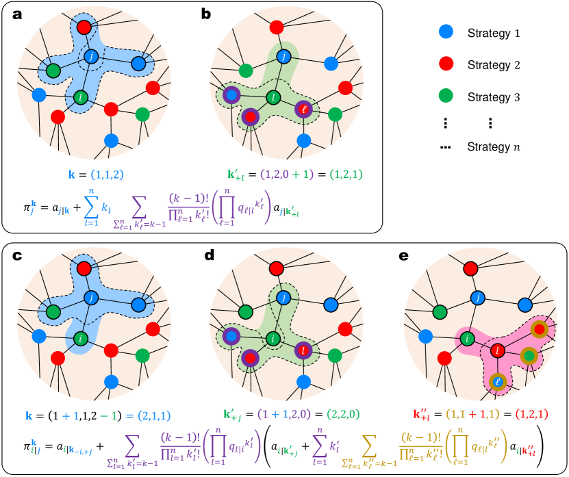
Figure E2: Visualization of the bottom-up statistical payoff calculation when every individual has $k=4$ neighbors. a, To calculate the expected payoff of a focal $j$-player with neighbor configuration $\mathbf{k}$, we first have the game organized by the $j$-player itself, with $\mathbf{k}$ as the co-player configuration. b, Then, we have $\sum_{l=1}^{n}k_{l}=k$ games organized by the $j$-player’s neighbors who adopt strategy $l=1,2,\dots,n$. For the $j$-player, the co-player configuration contains $k-1$ undetermined co-players neighboring the $l$-player, plus the $l$-player. c, To calculate the expected payoff of an $i$-player neighboring a focal $j$-player, with $j$-player’s neighbor configuration $\mathbf{k}$, we first have the game organized by the $j$-player. For the $i$-player, the co-player configuration is $\mathbf{k}_{-i,+j}$. d, Then, we have the game organized by the $i$-player itself, with $k-1$ undetermined co-players neighboring the $i$-player plus the $j$-player. e, Finally, we have the games organized by the $i$-player’s remaining $\sum_{l=1}^{n}k^{\prime}_{l}=k-1$ neighbors. For the $i$-player, the co-player configuration contains $k-1$ undetermined co-players neighboring the $l$-player, plus the $l$-player.

The $j$-player accumulates payoff from the games organized by itself and its $\sum_{l=1}^{n}k_{l}=k$ neighbors. The visualization of Eq. (8) is shown in Fig. E2a and b. Similarly, the expected payoff of an $i$-player neighboring a $j$-player, given the $j$-player’s neighbor configuration $\mathbf{k}$, can be expressed and calculated by

$$\pi_{i|j}^{\mathbf{k}}=a_{i|\mathbf{k}_{-i,+j}}+\sum_{\sum_{l=1}^{n}k^{\prime}_{l}=k-1}\frac{(k-1)!}{\prod_{l=1}^{n}k^{\prime}_{l}!}\left(\prod_{l=1}^{n}{q_{l|i}}^{k^{\prime}_{l}}\right)\left(a_{i|\mathbf{k}^{\prime}_{+j}}+\sum_{l=1}^{n}k^{\prime}_{l}\sum_{\sum_{\ell=1}^{n}k^{\prime\prime}_{\ell}=k-1}\frac{(k-1)!}{\prod_{\ell=1}^{n}k^{\prime\prime}_{\ell}!}\left(\prod_{\ell=1}^{n}{q_{\ell|l}}^{k^{\prime\prime}_{\ell}}\right)a_{i|\mathbf{k}^{\prime\prime}_{+l}}\right).$$ (9)

The $i$-player accumulated payoff from the games organized by the $j$-player (Fig. E2c), by itself (Fig. E2d), and by its remaining $\sum_{l=1}^{n}k^{\prime}_{l}=k-1$ neighbors (Fig. E2e). Further explanations of Eqs. (8) and (9) can be found in Supplementary Information.

Based on the microscopic quantities given specific $\mathbf{k}$, we can further express statistical quantities over all possible $\mathbf{k}$. The expected payoff of a focal $X$-player over all possible $\mathbf{k}$ can be statistically computed as

$$\langle\pi_{X}^{\mathbf{k}}\rangle=\sum_{\sum_{i^{\prime}=1}^{n}k_{i^{\prime}}=k}\frac{k!}{\prod_{i^{\prime}=1}^{n}k_{i^{\prime}}!}\left(\prod_{i^{\prime}=1}^{n}{q_{{i^{\prime}}|X}}^{k_{i^{\prime}}}\right)\pi_{X}^{\mathbf{k}}.$$ (10)

The possible neighbor configurations satisfying $\sum_{i^{\prime}=1}^{n}k_{i^{\prime}}=k$ are found around the $X$-player as identified by $q_{i^{\prime}|X}$. Here, $i^{\prime}$ is an independent count, which has no relation with $i$.

Similarly, the expected payoff of an $i$-player neighboring an $X$-player over all possible neighbor configuration $\mathbf{k}_{+i}$ of the $X$-player can be expressed as

$$\langle\pi_{i|X}^{\mathbf{k}_{+i}}\rangle=\sum_{\sum_{i^{\prime}=1}^{n}k_{i^{\prime}}=k-1}\frac{(k-1)!}{\prod_{i^{\prime}=1}^{n}k_{i^{\prime}}!}\left(\prod_{i^{\prime}=1}^{n}{q_{{i^{\prime}}|X}}^{k_{i^{\prime}}}\right)\pi_{i|X}^{\mathbf{k}_{+i}}.$$ (11)

Here, $\mathbf{k}_{+i}$ is because we have a specific $i$-player in the neighbor configuration of the $X$-player. The remaining $k-1$ neighbors $\sum_{i^{\prime}=1}^{n}k_{i^{\prime}}=k-1$ of the $X$-player are found around the $X$-player, as identified by $q_{i^{\prime}|X}$.

Eqs. (9) and (11) may seem redundant because they do not appear directly in the final results. However, they are crucial in the process of deductions for both pairwise comparison and death-birth rules.

We also have the similar notation for the statistical mean payoff at the single game level. To specify, the expected payoff of an $i$-player in a single game over all co-player configuration $\mathbf{k}$, where $\mathbf{k}$ is found neighboring an $X$-player, is expressed as

$$\langle a_{i|\mathbf{k}}\rangle_{X}=\sum_{\sum_{i^{\prime}=1}^{n}k_{i^{\prime}}=k}\frac{k!}{\prod_{i^{\prime}=1}^{n}k_{i^{\prime}}!}\left(\prod_{i^{\prime}=1}^{n}{q_{{i^{\prime}}|X}}^{k_{i^{\prime}}}\right)a_{i|\mathbf{k}}.$$ (12)

The concepts in Eqs. (8)–(12) are sufficient to identify the difference between this work and the previous literature. In particular, they emphasize that the minimal unit to refer is the co-player configuration $\mathbf{k}$, based on which the payoff of the multiplayer game can be computed. We do not try to decompose the multi-body interaction identified by $\mathbf{k}$ into multiple pairwise interactions.

Combined with the traditional pair approximation methods and some detailed calculations in the strategy evolution dynamics, we can then obtain the master equation (4) in the main text (see Supplementary Information section S2.4.3 for the approach of pair approximation deduction).

The decomposition to single games

The following form of the master equation is important, which holds for any $n$-strategy multiplayer game and allows us to obtain the replicator dynamics by summing the results from the mean payoff of a series of single games:

$$\dot{x}_{i}=\frac{\delta(k-2)}{2(k-1)}x_{i}\sum_{j=1}^{n}x_{j}\Bigg{(}\langle a_{i|\mathbf{k}_{+j}}\rangle_{i}+(k-1)\langle a_{i|\mathbf{k}_{+j}}\rangle_{j}+\langle a_{i|\mathbf{k}_{+i}}\rangle_{i}-\langle a_{j|\mathbf{k}_{+i}}\rangle_{j}-\langle a_{j|\mathbf{k}_{+i}}\rangle_{i}-(k-2)\sum_{j=1}^{n}x_{l}\langle a_{j|\mathbf{k}_{+l}}\rangle_{l}-\langle a_{j|\mathbf{k}_{+j}}\rangle_{j}\Bigg{)}.$$ (13)

In application, given the payoff functions $a_{i|\mathbf{k}}$ where $i=1,2,\dots,n$, we can compute all $\langle\cdot\rangle$ terms and then ensemble them to obtain the replicator equation. The result of each $\langle\cdot\rangle$ should be a function of $x_{1},x_{2},\dots,x_{n}$ (transformed from $q_{j|i}$ manually), degree $k$, and game parameters.

The advantage of Eq. (13) is that we have attributed everything about $\langle\cdot\rangle$ into two types, the ‘$\langle a_{i|\mathbf{k}_{+j}}\rangle_{i}$ type’ and the ‘$\langle a_{i|\mathbf{k}_{+j}}\rangle_{j}$ type’. They can be expressed by matrices through $i$ and $j$:

• The $\langle a_{i|\mathbf{k}_{+j}}\rangle_{i}$ type:

  $$\left[\langle a_{i|\mathbf{k}_{+j}}\rangle_{i}\right]_{ij}=\displaystyle{\begin{pmatrix}\langle a_{1|\mathbf{k}_{+1}}\rangle_{1}&\langle a_{1|\mathbf{k}_{+2}}\rangle_{1}&\cdots&\langle a_{1|\mathbf{k}_{+n}}\rangle_{1}\\ \langle a_{2|\mathbf{k}_{+1}}\rangle_{2}&\langle a_{2|\mathbf{k}_{+2}}\rangle_{2}&\cdots&\langle a_{2|\mathbf{k}_{+n}}\rangle_{2}\\ \vdots&\vdots&\ddots&\vdots\\ \langle a_{n|\mathbf{k}_{+1}}\rangle_{n}&\langle a_{n|\mathbf{k}_{+2}}\rangle_{n}&\cdots&\langle a_{n|\mathbf{k}_{+n}}\rangle_{n}\end{pmatrix}}.$$ (14)

• The $\langle a_{i|\mathbf{k}_{+j}}\rangle_{j}$ type:

  $$\left[\langle a_{i|\mathbf{k}_{+j}}\rangle_{j}\right]_{ij}=\displaystyle{\begin{pmatrix}\langle a_{1|\mathbf{k}_{+1}}\rangle_{1}&\langle a_{1|\mathbf{k}_{+2}}\rangle_{2}&\cdots&\langle a_{1|\mathbf{k}_{+n}}\rangle_{n}\\ \langle a_{2|\mathbf{k}_{+1}}\rangle_{1}&\langle a_{2|\mathbf{k}_{+2}}\rangle_{2}&\cdots&\langle a_{2|\mathbf{k}_{+n}}\rangle_{n}\\ \vdots&\vdots&\ddots&\vdots\\ \langle a_{n|\mathbf{k}_{+1}}\rangle_{1}&\langle a_{n|\mathbf{k}_{+2}}\rangle_{2}&\cdots&\langle a_{n|\mathbf{k}_{+n}}\rangle_{n}\end{pmatrix}}.$$ (15)

In this way, we attribute the computation to these two types, before substituting them to Eq. (13). There are $n^{2}$ elements in each matrix. Their diagonals are equal, meaning we can compute $n$ fewer elements. Therefore, the total amount of computation is $n^{2}+n^{2}-n=(2n-1)n$ elements. The computational complexity is $\mathrm{O}(n^{2})$, which can be accomplished in polynomial time (we will also see that the death-birth rule’s computational complexity is $\mathrm{O}(n^{3})$, as specified in Supplementary Information).

Special linear system

Although Eq. (13) allows general calculations of any multiplayer game, we do not have to employ it directly every time. For some special payoff structures, we can deduce more convenient forms in advance. Here, we present the general results of a commonly studied subclass, the linear multiplayer games.

The linear multiplayer games in this work are defined as those whose payoff structure can be expressed as linear functions of co-player configuration $\mathbf{k}=k_{1},k_{2},\dots,k_{n}$. That is, $a_{i|\mathbf{k}}=\sum_{j=1}^{n}b_{ij}k_{j}+c_{i}$, where

$$\mathbf{b}=\begin{pmatrix}b_{11}&b_{12}&\cdots&b_{1n}\\ b_{21}&b_{22}&\cdots&b_{2n}\\ \vdots&\vdots&\ddots&\vdots\\ b_{n1}&b_{n2}&\cdots&b_{nn}\end{pmatrix},\leavevmode\nobreak\ \mathbf{c}=\begin{pmatrix}c_{1}\\ c_{2}\\ \vdots\\ c_{n}\end{pmatrix}.$$ (16)

For linear multiplayer games, the payoff structure is completely determined by the matrix $\mathbf{b}$ and $\mathbf{c}$.

Once we apply $a_{i|\mathbf{k}}=\sum_{j=1}^{n}b_{ij}k_{j}+c_{i}$ to compute the ‘$\langle a_{i|\mathbf{k}_{+j}}\rangle_{i}$ type’ and the ‘$\langle a_{i|\mathbf{k}_{+j}}\rangle_{j}$ type’ as shown in Eqs. (14) and (15) and transform all $q_{j|i}$ quantities to $x_{j}$ quantities, we can obtain $\langle a_{i|\mathbf{k}_{+j}}\rangle_{i}=(k-2)\sum_{l=1}^{n}b_{il}x_{l}+b_{ii}+b_{ij}+c_{i}$, $\langle a_{i|\mathbf{k}_{+j}}\rangle_{j}=(k-2)\sum_{l=1}^{n}b_{il}x_{l}+2b_{ij}+c_{i}$. Then, substituting the results into Eq. (13) leads to Eq. (5) in the main text.

As we mentioned in the main text, in Eq. (5), $\bar{\pi}_{i}$ and $\bar{\pi}$ are the expected payoff of $i$-players and all players in a well-mixed population. They can be calculated by the traditional replicator dynamics, but to specify, using the matrix $\mathbf{b}$ and $\mathbf{c}$, they can be written as $\bar{\pi}_{i}=k\sum_{l=1}^{n}x_{l}b_{il}+c_{i}$, $\bar{\pi}=\sum_{i=1}^{n}x_{i}\pi_{i}=k\sum_{i=1}^{n}\sum_{l=1}^{n}x_{i}x_{l}b_{il}+\sum_{i=1}^{n}x_{i}c_{i}$. Logically, this is how we replace the corresponding terms in Eq. (5) by $\bar{\pi}_{i}$ and $\bar{\pi}$.

Peer punishment

According to the description in the main text, the payoff structure of public goods game with peer punishment is

$$a_{1|\mathbf{k}} =\frac{r(k_{1}+1+k_{3})c}{k+1}-c,$$ (17a)

$$a_{2|\mathbf{k}} =\frac{r(k_{1}+k_{3})c}{k+1}-\beta k_{3},$$ (17b)

$$a_{3|\mathbf{k}} =\frac{r(k_{1}+k_{3}+1)c}{k+1}-c-\alpha k_{2},$$ (17c)

where strategy 1, 2, 3 are cooperation ($C$), defection ($D$), and peer punishment ($E$). According to Eq. (17), we find the payoff structure is linear and can be determined by the following matrix $\mathbf{b}$ and $\mathbf{c}$:

$$\mathbf{b}=\begin{pmatrix}\dfrac{rc}{k+1}&0&\dfrac{rc}{k+1}\\[10.00002pt] \dfrac{rc}{k+1}&0&\dfrac{rc}{k+1}-\beta\\[10.00002pt] \dfrac{rc}{k+1}&-\alpha&\dfrac{rc}{k+1}\end{pmatrix},\leavevmode\nobreak\ \mathbf{c}=\begin{pmatrix}\dfrac{rc}{k+1}-c\\[10.00002pt] 0\\ \dfrac{rc}{k+1}-c\end{pmatrix}.$$ (18)

In this way, we can utilize Eq. (5) to obtain the replicator equation in structured populations:

$$\dot{x}_{1} =\frac{\delta(k-2)}{2(k-1)}x_{1}\left\{(k+1)\left[(1-x_{1}-x_{3})\left(\frac{rc}{k+1}-c\right)+kx_{2}x_{3}(\alpha+\beta)\right]-6x_{2}x_{3}(\alpha+\beta)\right\},$$ (19a)

$$\dot{x}_{2} =\frac{\delta(k-2)}{2(k-1)}x_{2}\left\{(k+1)\left[-(x_{1}+x_{3})\left(\frac{rc}{k+1}-c\right)+k\left(x_{2}x_{3}(\alpha+\beta)-x_{3}\beta\right)\right]-6x_{2}x_{3}(\alpha+\beta)+3x_{3}(\alpha+\beta)\right\},$$ (19b)

$$\dot{x}_{3} =\frac{\delta(k-2)}{2(k-1)}x_{3}\left\{(k+1)\left[(1-x_{1}-x_{3})\left(\frac{rc}{k+1}-c\right)+k\left(x_{2}x_{3}(\alpha+\beta)-x_{2}\alpha\right)\right]-6x_{2}x_{3}(\alpha+\beta)+3x_{2}(\alpha+\beta)\right\}.$$ (19c)

By standard analysis (see Supplementary Information, which also trivially analyzes well-mixed populations), we can obtain all details about equilibrium and the stability of system (19). The main results are summarized in Fig. E3.

Pool punishment

According to the description in the main text, the payoff structure of public goods game with pool punishment is

$$a_{1|\mathbf{k}} =\frac{r(k_{1}+1+k_{3})c}{k+1}-c=\frac{rc}{k+1}k_{1}+\frac{rc}{k+1}k_{3}+\frac{rc}{k+1}-c,$$ (20a)

$$a_{2|\mathbf{k}} =\frac{r(k_{1}+k_{3})c}{k+1}-\beta f(k_{3})=\frac{rc}{k+1}k_{1}+\frac{rc}{k+1}k_{3}-\beta f(k_{3}),$$ (20b)

$$a_{3|\mathbf{k}} =\frac{r(k_{1}+k_{3}+1)c}{k+1}k_{1}-c-\alpha=\frac{rc}{k+1}k_{1}+\frac{rc}{k+1}k_{3}+\frac{rc}{k+1}-c-\alpha,$$ (20c)

where strategy 1, 2, 3 are cooperation ($C$), defection ($D$), and pool punishment ($O$); $f(k_{3})=1$ if $k_{3}>0$ (indicating the presence of punisher co-players) and $f(k_{3})=0$ if $k_{3}=0$ (indicating no punisher co-players). The payoff structure of Eq. (17) is not linear. Therefore, let us proceed it with the general Eq. (13), summing the results from the mean payoff of a series of single games in the ‘$\langle a_{i|\mathbf{k}_{+j}}\rangle_{i}$ type’ and the ‘$\langle a_{i|\mathbf{k}_{+j}}\rangle_{j}$ type’. By detailed calculation listed in Supplementary Information, we obtain

$$\dot{x}_{1} =\frac{\delta(k-2)(k+1)}{2(k-1)}x_{1}\left\{(1-x_{1}-x_{3})\left(\frac{rc}{k+1}-c\right)+x_{3}\alpha+(1-x_{1}-x_{3})\beta\left[1-\left(1-\frac{k-2}{k+1}x_{3}\right)\left(1-\frac{k-2}{k-1}x_{3}\right)^{k-1}\right]\right\},$$ (21a)

$$\dot{x}_{3} =\frac{\delta(k-2)(k+1)}{2(k-1)}x_{3}\left\{(1-x_{1}-x_{3})\left(\frac{rc}{k+1}-c\right)-(1-x_{3})\alpha+(1-x_{1}-x_{3})\beta\left[1-\frac{k-1}{k+1}\left(1-\frac{k-2}{k-1}x_{3}\right)^{k}\right]\right\},$$ (21b)

and $\dot{x}_{2}=-\dot{x}_{1}-\dot{x}_{3}$. Then, by similar standard analysis, we obtain all details about equilibrium and the stability of system (21). The main results are summarized in Fig. E4.

Death-birth and the comparison with $n=2$

Without loss of generality, here we present the results of another representative strategy update rule, the death-birth (DB) [29]. During an elementary step, the randomly selected focal individual from the population dies and its neighbors reproduce their strategy to the vacancy with probability proportional to their fitness. Using the same payoff expression but apply different strategy dynamics (see Supplementary Information), we obtain the following replicator equation for $i=1,2,\dots,n$.

$$\dot{x}_{i}=\frac{\delta(k-1)}{k}x_{i}\left(\langle\pi_{i}^{\mathbf{k}}\rangle-\sum_{j=1}^{n}\sum_{i^{\prime}=1}^{n}q_{i^{\prime}|j}q_{j|i}\langle\pi_{i^{\prime}|j}^{\mathbf{k}_{+i,+i^{\prime}}}\rangle\right),$$ (22)

Eq. (22) bears an intuitive interpretation if we consider the following two concepts: (1) $\pi_{i}^{(0)}=\langle\pi_{i}^{\mathbf{k}}\rangle$, the expected accumulated payoff of the $i$-player itself (zero-step away on the graph), and (2) $\pi_{i}^{(2)}=\sum_{j=1}^{n}\sum_{i^{\prime}=1}^{n}q_{i^{\prime}|j}q_{j|i}\langle\pi_{i^{\prime}|j}^{\mathbf{k}_{+i,+i^{\prime}}}\rangle$, the expected accumulated payoff of the $i$-player’s second-order neighbors (i.e., neighbor’s neighbor, two-step away on the graph). In this way, it is indicated from Eq. (22) that $\dot{x}_{i}\sim x_{i}(\pi_{i}^{(0)}-\pi_{i}^{(2)})$. The essence of death-birth is the competition between oneself and its second-order neighbors, which is consistent with the observation from the IBD idea [18]. Here, we further extend the idea to $n$-strategy systems in infinite populations by replicator dynamics.

Previously, Li et al. [44] found the general replicator equation for any 2-strategy multiplayer game on regular graphs under the death-birth rule. Their results can also be obtained by taking $n=2$ in our Eq. (22). After transformation and simplification (see Supplementary Information section A.5), we find that $n=2$ in Eq. (22) results in

$$\dot{x}_{1}= \leavevmode\nobreak\ \frac{\delta(k-2)}{k(k-1)}x_{1}(1-x_{1})\Big{\{}k\left(\langle\pi_{1|2}^{\mathbf{k}_{+1,+2}}\rangle-\langle\pi_{2|2}^{\mathbf{k}_{+1,+2}}\rangle\right)$$

$$+[(k-2)x_{1}+1]\left[\left(\langle\pi_{1|1}^{\mathbf{k}_{+1,+2}}\rangle-\langle\pi_{2|1}^{\mathbf{k}_{+1,+2}}\rangle\right)-\left(\langle\pi_{1|2}^{\mathbf{k}_{+1,+2}}\rangle-\langle\pi_{2|2}^{\mathbf{k}_{+1,+2}}\rangle\right)\right]\Big{\}},$$ (23)

and $\dot{x}_{2}=-\dot{x}_{1}$. Eq. (Death-birth and the comparison with $n=2$) is the complete form of the result obtained in by Li et al. [44]. In particular, we further clarify that the calculation in each $\langle\cdot\rangle$ should be made in the remaining $k-2$ individuals given the existence of at least a pair of 1-player and 2-player.

For the decomposition to single games under the death-birth rule, which is rather complicated, the readers can refer to Supplementary Information section A.4.2.

Finally, for special linear system where the payoff is a linear function of co-player number, $a_{i|\mathbf{k}}=\sum_{j=1}^{n}b_{ij}k_{j}+c_{i}$, the replicator equation under the death-birth rule can be expressed as

$$\dot{x}_{i}=\frac{\delta(k-2)}{k(k-1)^{2}}x_{i}\left\{\frac{(k^{2}-2)^{2}}{k}(\bar{\pi}_{i}-\bar{\pi})+\frac{3k^{2}-4}{k}\left((kb_{ii}+c_{i})-\sum_{j=1}^{n}x_{j}(kb_{jj}+c_{j})\right)-(k^{2}+2k-4)\sum_{j=1}^{n}x_{j}\left(b_{ji}-\sum_{l=1}^{n}x_{l}b_{jl}\right)\right\},$$ (24)

where $\bar{\pi}_{i}$ and $\bar{\pi}$ are the mean payoff of $i$-players and all players in a well-mixed population.

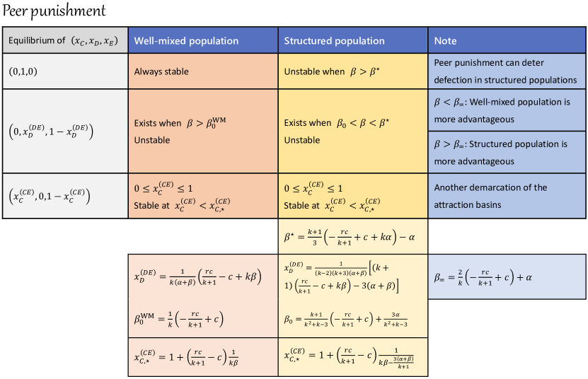
Figure E3: Analytical results of public goods game with peer punishment in both well-mixed and structured populations. This table summarizes the equilibrium points and their stability by analyzing system (19). The analytical forms of all key concepts are presented. See Supplementary Information section S3.2 for details of the analysis.

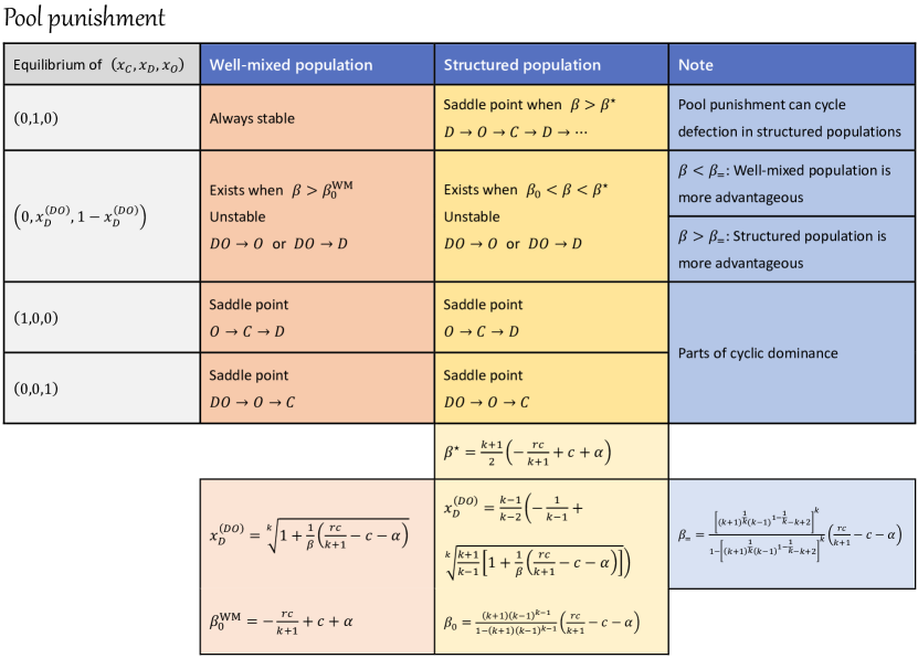
Figure E4: Analytical results of public goods game with pool punishment in both well-mixed and structured populations. This table summarizes the equilibrium points and their stability by analyzing system (21). The analytical forms of all key concepts are presented. See Supplementary Information section S3.3 for details of the analysis.

S1 System construction and payoff calculation on a regular graph

We employ the pair approximation method [29, 33, 44, 24, 26] to deduce the system dynamics. First, we express the system and explain the payoff calculation in detail.

S1.1 Expressing the system

On the regular graph of degree $k$, the number of nodes is $N$ and the number of edges is $kN/2$, where the population size $N\to+\infty$. In this infinite population, the proportion of individuals who choose strategy $i$ is denoted by $x_{i}$. The probability of finding a $j$-player neighboring an $i$ player is denoted by $q_{j|i}$. The proportion of indirected $ij$-edges connecting a pair of strategy $i$ and $j$ is denoted by $p_{ij}$.

To sum up, there are $n+n^{2}+n^{2}$ variables to describe the system: $n$ for $x_{i}$, $n^{2}$ for $q_{j|i}$, and $n^{2}$ for $p_{ij}$. They yield the following constraints.

$$\sum_{i=1}^{n}x_{i} =1,$$

$$\sum_{j=1}^{n}q_{j|i} =1,\quad\text{for $i=1,2,\dots,n$},$$

$$p_{ij} =x_{i}q_{j|i},\quad\text{for $i=1,2,\dots,n$, $j=1,2,\dots,n$},$$

$$p_{ij} =p_{ji},\quad\text{for $i=1,2,\dots,n$, $j=1,2,\dots,n$, $i\neq j$}.$$ (S1)

According to the third line in Eq. (S1.1), the system can be described by $x_{i}$ and $q_{j|i}$, eliminating the need to use $p_{ij}$.

S1.2 Payoff calculation of a $j$-player

As mentioned in the main text, to express a $j$-player’s accumulated payoff, received from the multiplayer games organized by itself and neighbors, we need to introduce a variant of neighbor configuration $\mathbf{k}$ as follows.

$$\mathbf{k}_{+j}=(k_{1},k_{2},\dots,k_{j}+1,\dots,k_{n}),$$ (S2)

where $\sum_{l=1}^{n}k_{l}=k-1$. This notation describes a configuration which has two components: (i) one individual chooses strategy $j$; (ii) among $k-1$ remaining individuals, $k_{1},k_{2},\dots,k_{j},\dots,k_{n}$ individuals choose strategy $1,2,\dots,j,\dots,n$. Here, $j$ could be an integer satisfying $1\leq j\leq n$.

Consider a focal $j$-player with neighbor configuration $\mathbf{k}$. Then, the accumulated payoff of this $j$-player, denoted by $\pi_{j}^{\mathbf{k}}$, can be expressed as

$$\pi_{j}^{\mathbf{k}}=a_{j|\mathbf{k}}+\sum_{l=1}^{n}k_{l}\sum_{\sum_{\ell=1}^{n}k^{\prime}_{\ell}=k-1}\frac{(k-1)!}{\prod_{\ell=1}^{n}k^{\prime}_{\ell}!}\left(\prod_{\ell=1}^{n}{q_{\ell|l}}^{k^{\prime}_{\ell}}\right)a_{j|\mathbf{k}^{\prime}_{+l}}.$$ (S3)

It is straightforward that $a_{j|\mathbf{k}}$ is the payoff received from the game organized by the $j$-player itself. Furthermore, in the $j$-player’s neighbor configuration $\mathbf{k}$, there are $k_{l}$ individuals with strategy $l$.

In the game organized by an $l$-player, there must be a $j$-player, the focal player. We denote the neighbor configuration of the $l$-player as $\mathbf{k}^{\prime}_{+j}$, where the upper right prime (^′) is only to distinguish from $\mathbf{k}$. Here, $\mathbf{k}^{\prime}_{+j}$ contains the focal $j$-player and the remaining $k-1$ uncertain $\ell$-players, determined by going through $\sum_{\ell=1}^{n}k^{\prime}_{\ell}=k-1$. Given that the $l$-player’s co-player configuration in its own group is $\mathbf{k}^{\prime}_{+j}$, the focal $j$-player’s co-player configuration in the same group is then expressed as $\mathbf{k}^{\prime}_{+l}$: removing itself and adding the $l$-player. As a result, $\mathbf{k}^{\prime}_{+l}$ contains the $l$-player and the remaining $k-1$ uncertain $\ell$-players. Therefore, the $j$-player receives payoff $a_{j|\mathbf{k}^{\prime}_{+l}}$ from the games organized by each $l$-player neighbor by determining the remaining $k-1$ uncertain $\ell$-co-players in $\mathbf{k}^{\prime}_{+l}$.

S1.3 Payoff calculation of an $i$-player neighboring a $j$-player

Now we consider a more complex case, the accumulated payoff of an $i$-player neighboring a focal $j$-player. To express the accumulated payoff of the $i$-player, we need to further introduce a variant of $\mathbf{k}$ as follows.

$$\mathbf{k}_{-i,+j}=(k_{1},k_{2},\dots,k_{i}-1,\dots,k_{j}+1,\dots,k_{n}),$$ (S4)

where $\sum_{l=1}^{n}k_{l}=k$. This notation describes a variant to the configuration $\mathbf{k}$, with one less individual choosing strategy $i$, and one more individual choosing strategy $j$. Here, $i$ and $j$ could be integers, satisfying $1\leq i\leq n$ and $1\leq j\leq n$. Moreover, the order of $i$ and $j$ ($i<j$ or $i>j$) does not matter in $\mathbf{k}_{-i,+j}$.

Again, we consider a focal $j$-player with neighbor configuration $\mathbf{k}$. The expected payoff of an $i$-player neighboring this focal $j$-player can be expressed as

$$\pi_{i|j}^{\mathbf{k}}=a_{i|\mathbf{k}_{-i,+j}}+\sum_{\sum_{l=1}^{n}k^{\prime}_{l}=k-1}\frac{(k-1)!}{\prod_{l=1}^{n}k^{\prime}_{l}!}\left(\prod_{l=1}^{n}{q_{l|i}}^{k^{\prime}_{l}}\right)\left(a_{i|\mathbf{k}^{\prime}_{+j}}+\sum_{l=1}^{n}k^{\prime}_{l}\sum_{\sum_{\ell=1}^{n}k^{\prime\prime}_{\ell}=k-1}\frac{(k-1)!}{\prod_{\ell=1}^{n}k^{\prime\prime}_{\ell}!}\left(\prod_{\ell=1}^{n}{q_{\ell|l}}^{k^{\prime\prime}_{\ell}}\right)a_{i|\mathbf{k}^{\prime\prime}_{+l}}\right).$$ (S5)

In Eq. (S5), $a_{i|\mathbf{k}_{-i,+j}}$ is the payoff received from the game organized by the focal $j$-player. Note that $\mathbf{k}$ describes the neighbor configuration of the $j$-player. Therefore, $i$-player joining the game organized by the focal $j$-player, the remaining participants’ configuration for this $i$-player becomes $\mathbf{k}_{-i,+j}$.

Let $\mathbf{k}^{\prime}_{+j}$ denote the $i$-player’s neighbor configuration. There are one neighbor employing strategy $j$, the focal $j$-player. The remaining $k-1$ neighbors are undetermined. Therefore, we go through $\sum_{l=1}^{n}k^{\prime}_{l}=k-1$ for all possibilities of $\mathbf{k}^{\prime}_{+j}$. In the game organized by the $i$-player itself, the payoff can be expressed as $a_{i|\mathbf{k}^{\prime}_{+j}}$.

Among the $i$-player’s remaining $k-1$ neighbors, the number of $l$-players is $k_{l}^{\prime}$. We denote an $l$-player’s neighbor configuration by $\mathbf{k}_{+i}^{\prime\prime}$: the $i$-player’s strategy $i$ is determined, and the remaining $k-1$ players are undetermined. We go through $\sum_{\ell=1}^{n}k_{\ell}^{\prime\prime}=k-1$ for all possibilities. While the configuration of other players around the $l$-player is $\mathbf{k}_{+i}^{\prime\prime}$, the configuration around the $i$-player should be rewritten by $\mathbf{k}^{\prime\prime}_{+l}$: removing the $i$-player and adding the $l$-player. Therefore, in the game organized by an $l$-player neighboring the $i$-player, the payoff of the $i$-player is $a_{i|\mathbf{k}_{+l}^{\prime\prime}}$.

Knowing the payoff calculation, we can study the evolutionary dynamics. Here, we investigate two update rules for the evolution of strategies, pairwise comparison and death-birth, presented in section S2 and Appendix A, respectively.

S2 Pairwise comparison

In a unit time, a random focal individual is selected to update the strategy by comparing the fitness with a random neighbor. Suppose that the focal individual $A$ compares its fitness with the neighbor $B$. The individual $A$ adopts the strategy of $B$ with the following probability:

$$W=\frac{F_{B}}{F_{A}+F_{B}}.$$ (S6)

Otherwise, individual $A$ keeps its own strategy in the remaining probability $F_{A}/(F_{A}+F_{B})$. Here, $F_{A}$ and $F_{B}$ is the fitness of the individual $A$ and $B$. As mentioned in the main text, the transformation from payoff to fitness is $F=\exp{(\delta\pi)}$ [21, 46]. In this way, the adopting probability $W$ has the following well-known form [55]:

$$W=\frac{1}{1+\exp{[-\delta(\pi_{B}-\pi_{A})]}},$$ (S7)

where $\pi_{A}$ and $\pi_{B}$ is the fitness of individual $A$ and $B$, and $\delta\to 0^{+}$ is the weak selection strength. According to Eq. (S7), if individual $B$ has a higher payoff, then its strategy has a slightly higher probability to be adopted by individual $A$.

Below, we analyze the strategy evolution under pairwise comparison.

S2.1 The increase of $i$-players

The increase of $i$-players happens when a focal $j$-player ($j\neq i$) is selected to update its strategy and an $i$-player takes the position. Given the focal $j$-player’s neighbor configuration $\mathbf{k}$, the probability that an $i$-player takes the $j$-player’s position is

$$\mathcal{P}(j\leftarrow i)=\frac{k_{i}}{k}\frac{F_{i|j}^{\mathbf{k}}}{F_{j}^{\mathbf{k}}+F_{i|j}^{\mathbf{k}}}=\frac{k_{i}}{2k}+\frac{k_{i}}{4k}(\pi_{i|j}^{\mathbf{k}}-\pi_{j}^{\mathbf{k}})\delta+\mathcal{O}(\delta^{2}).$$ (S8)

The randomly selected neighbor from $\mathbf{k}$ is an $i$-player with probability $k_{i}/k$. Then, the focal $j$-player adopts the $i$-player’s strategy with the probability of pairwise comparison. Taylor expansion at $\delta\to 0^{+}$ has been performed in Eq. (S8).

Then, we apply Eq. (S8) to all possibilities for $j\neq i$ and the neighbor configuration $\mathbf{k}$, obtaining the probability that the number of $i$-players increases by 1 (i.e., the frequency of $i$-players increases by $1/N$) during a unit time step,

$$\mathcal{P}\left(\Delta x_{i}=\frac{1}{N}\right) =\sum_{j=1,j\neq i}^{n}x_{j}\sum_{\sum_{i^{\prime}=1}^{n}k_{i^{\prime}}=k}\frac{k!}{\prod_{i^{\prime}=1}^{n}k_{i^{\prime}}!}\left(\prod_{i^{\prime}=1}^{n}{q_{i^{\prime}|j}}^{k_{i^{\prime}}}\right)\mathcal{P}(j\leftarrow i)$$

$$=\frac{1}{2}\sum_{j=1,j\neq i}^{n}x_{j}q_{i|j}+\frac{1}{4}\sum_{j=1,j\neq i}^{n}x_{j}\sum_{\sum_{i^{\prime}=1}^{n}k_{i^{\prime}}=k}\frac{k!}{\prod_{i^{\prime}=1}^{n}k_{i^{\prime}}!}\left(\prod_{i^{\prime}=1}^{n}{q_{i^{\prime}|j}}^{k_{i^{\prime}}}\right)\frac{k_{i}}{k}\left(\pi_{i|j}^{\mathbf{k}}-\pi_{j}^{\mathbf{k}}\right)\delta+\mathcal{O}(\delta^{2}),$$ (S9)

where the notation $i^{\prime}$ is independent, only to distinguish from $i$.

S2.2 The decrease of $i$-players

The decrease of $i$-players happens when a focal $i$-player is selected to update its strategy and the player who takes the position is not an $i$-player. Given the focal $i$-player’s neighbor configuration $\mathbf{k}$, the probability that the player who takes the position is not an $i$-player is

$$\sum_{j=1,j\neq i}^{n}\mathcal{P}(i\leftarrow j)=\sum_{j=1,j\neq i}^{n}\frac{k_{j}}{k}\frac{F_{j|i}^{\mathbf{k}}}{F_{i}^{\mathbf{k}}+F_{j|i}^{\mathbf{k}}}=\frac{k-k_{i}}{2k}+\sum_{j=1,j\neq i}^{n}\frac{k_{j}}{4k}(\pi_{j|i}^{\mathbf{k}}-\pi_{i}^{\mathbf{k}})\delta+\mathcal{O}(\delta^{2}).$$ (S10)

Applying it to all possibilities for the neighbor configuration $\mathbf{k}$ after selecting a focal $i$-player with probability $x_{i}$, we obtain the probability that the number of $i$-players decreases by 1 during a unit time step,

$$\mathcal{P}\left(\Delta x_{i}=-\frac{1}{N}\right) =x_{i}\sum_{\sum_{i^{\prime}=1}^{n}k_{i^{\prime}}=k}\frac{k!}{\prod_{i^{\prime}=1}^{n}k_{i^{\prime}}!}\left(\prod_{i^{\prime}=1}^{n}{q_{i^{\prime}|i}}^{k_{i^{\prime}}}\right)\sum_{j=1,j\neq i}^{n}\mathcal{P}(i\leftarrow j)$$

$$=\frac{x_{i}(1-q_{i|i})}{2}+\frac{1}{4}x_{i}\sum_{\sum_{i^{\prime}=1}^{n}k_{i^{\prime}}=k}\frac{k!}{\prod_{i^{\prime}=1}^{n}k_{i^{\prime}}!}\left(\prod_{i^{\prime}=1}^{n}{q_{i^{\prime}|i}}^{k_{i^{\prime}}}\right)\sum_{j=1,j\neq i}^{n}\frac{k_{j}}{k}\left(\pi_{j|i}^{\mathbf{k}}-\pi_{i}^{\mathbf{k}}\right)\delta+\mathcal{O}(\delta^{2}).$$ (S11)

S2.3 The replicator equation

The instant change in the frequency $x_{i}$ of $i$-players consists of the increase and decrease of $i$-players. Applying Eqs. (S2.1) and (S2.2), and considering that a full Monte Carlo step contains $N$ elementary steps, we have

$$\dot{x}_{i}= \leavevmode\nobreak\ N\times\left\{\frac{1}{N}\mathcal{P}\left(\Delta x_{i}=\frac{1}{N}\right)+\left(-\frac{1}{N}\right)\mathcal{P}\left(\Delta x_{i}=-\frac{1}{N}\right)\right\}$$

$$= \leavevmode\nobreak\ \frac{1}{4}\sum_{j=1,j\neq i}^{n}x_{j}\sum_{\sum_{i^{\prime}=1}^{n}k_{i^{\prime}}=k}\frac{k!}{\prod_{i^{\prime}=1}^{n}k_{i^{\prime}}!}\left(\prod_{i^{\prime}=1}^{n}{q_{{i^{\prime}}|j}}^{k_{i^{\prime}}}\right)\frac{k_{i}}{k}\left(\pi_{i|j}^{\mathbf{k}}-\pi_{j}^{\mathbf{k}}\right)\delta$$

$$-\frac{1}{4}x_{i}\sum_{\sum_{i^{\prime}=1}^{n}k_{i^{\prime}}=k}\frac{k!}{\prod_{i^{\prime}=1}^{n}k_{i^{\prime}}!}\left(\prod_{i^{\prime}=1}^{n}{q_{i^{\prime}|i}}^{k_{i^{\prime}}}\right)\sum_{j=1,j\neq i}^{n}\frac{k_{j}}{k}\left(\pi_{j|i}^{\mathbf{k}}-\pi_{i}^{\mathbf{k}}\right)\delta+\mathcal{O}(\delta^{2}).$$ (S12)

In Eq. (S2.3), the $\delta^{0}$ term has been eliminated: applying Eq. (S1.1), we know $x_{j}q_{i|j}=p_{ij}=x_{i}q_{j|i}$ and $\sum_{j=1}^{n}q_{j|i}=1$, such that the $\delta^{0}$ term in Eq. (S2.1) can be expressed as $\frac{1}{2}\sum_{j=1,j\neq i}^{n}x_{j}q_{i|j}=\frac{1}{2}x_{i}\sum_{j=1,j\neq i}^{n}q_{j|i}=\frac{x_{i}(1-q_{i|i})}{2}$, which is equal to the one in Eq. (S2.1).

The $\delta^{0}$ term being eliminated, the instant change in $x_{i}$ happens on the order of $\delta^{1}$ (which is the reason we must perform the Taylor expansion to $\delta^{1}$ in Sections S2.1 and S2.2). Meanwhile, the instant change in $q_{i|j}$ for $i,j=1,2,\dots,n$ happens on the order of $\delta^{0}$ since the $\delta^{0}$ term is non-zero (see Appendix B.1). That is, the change in $q_{i|j}$ is much faster than $x_{i}$, so that $x_{i}$ changes on the basis of $q_{i|j}$ achieving equilibrium. According to Appendix B.1, we have the following solution when $q_{i|j}$ achieves stability.

$$q_{i|j}=\begin{cases}\displaystyle{\frac{k-2}{k-1}x_{i}},&j\neq i,\\ \\ \displaystyle{\frac{k-2}{k-1}x_{i}+\frac{1}{k-1}},&j=i.\end{cases}$$ (S13)

The primitive replicator equation of $x_{i}$ is Eq. (S2.3), where $\mathcal{O}(\delta^{2})=0$, $\pi_{j}^{\mathbf{k}}$ and $\pi_{i}^{\mathbf{k}}$ is given by Eq. (S3), $\pi_{i|j}^{\mathbf{k}}$ and $\pi_{j|i}^{\mathbf{k}}$ is given by Eq. (S5), and $q_{{i^{\prime}}|j}$ is given by Eq. (S13). The degrees of freedom of the replicator dynamics system are $n-1$, represented by independent variables $x_{i}$ ($i=1,2,\dots,n$, cancel one of them by $\sum_{i}^{n}x_{i}=1$).

S2.4 Simplification and discussion

The replicator equation given by Eq. (S2.3) can be further simplified and discussed. To do this, we need to introduce a useful equation, as given by Theorem 1 in Appendix C. For frequency quantities $0\leq z_{j}\leq 1$ and an arbitrary function $g(\mathbf{k})$ of vector $\mathbf{k}=(k_{1},k_{2},\dots,k_{n})$, we have:

$$\sum_{\sum_{j=1}^{n}k_{j}=k}\frac{k!}{\prod_{j=1}^{n}k_{j}!}\left(\prod_{j=1}^{n}{z_{j}}^{k_{j}}\right)k_{i}g(\mathbf{k})=kz_{i}\sum_{\sum_{j=1}^{n}k_{j}=k-1}\frac{(k-1)!}{\prod_{j=1}^{n}k_{j}!}\left(\prod_{j=1}^{n}{z_{j}}^{k_{j}}\right)g(\mathbf{k}_{+i}),$$ (S14)

which simplifies the expression by canceling the quantity $k_{i}$ in the summation at the cost of changing $f(\mathbf{k})$ to $f(\mathbf{k}_{+i})$.

S2.4.1 The accumulated payoff level

Using Eq. (S14), we can simplify the replicator equation (S2.3) to the accumulated payoff level. That is, we can obtain an equation to avoid specific calculations of $k_{i}$ in front of $\pi_{i|j}^{\mathbf{k}}$ and $\pi_{j}^{\mathbf{k}}$. The simplified replicator equation is

$$\dot{x}_{i}= \leavevmode\nobreak\ \frac{\delta}{4}\sum_{j=1,j\neq i}^{n}x_{j}q_{i|j}\sum_{\sum_{i^{\prime}=1}^{n}k_{i^{\prime}}=k-1}\frac{(k-1)!}{\prod_{i^{\prime}=1}^{n}k_{i^{\prime}}!}\left(\prod_{i^{\prime}=1}^{n}{q_{{i^{\prime}}|j}}^{k_{i^{\prime}}}\right)\left(\pi_{i|j}^{\mathbf{k}_{+i}}-\pi_{j}^{\mathbf{k}_{+i}}\right)$$

$$\leavevmode\nobreak\ -\frac{\delta}{4}x_{i}\sum_{\sum_{i^{\prime}=1}^{n}k_{i^{\prime}}=k-1}\frac{(k-1)!}{\prod_{i^{\prime}=1}^{n}k_{i^{\prime}}!}\left(\prod_{i^{\prime}=1}^{n}{q_{i^{\prime}|i}}^{k_{i^{\prime}}}\right)\sum_{j=1,j\neq i}^{n}q_{j|i}\left(\pi_{j|i}^{\mathbf{k}_{+j}}-\pi_{i}^{\mathbf{k}_{+j}}\right)$$

$$= \leavevmode\nobreak\ \frac{\delta}{4}x_{i}\sum_{j=1,j\neq i}^{n}q_{j|i}\sum_{\sum_{i^{\prime}=1}^{n}k_{i^{\prime}}=k-1}\frac{(k-1)!}{\prod_{i^{\prime}=1}^{n}k_{i^{\prime}}!}\left(\prod_{i^{\prime}=1}^{n}{q_{{i^{\prime}}|j}}^{k_{i^{\prime}}}\right)\left(\pi_{i|j}^{\mathbf{k}_{+i}}-\pi_{j}^{\mathbf{k}_{+i}}\right)$$

$$\leavevmode\nobreak\ -\frac{\delta}{4}x_{i}\sum_{j=1,j\neq i}^{n}q_{j|i}\sum_{\sum_{i^{\prime}=1}^{n}k_{i^{\prime}}=k-1}\frac{(k-1)!}{\prod_{i^{\prime}=1}^{n}k_{i^{\prime}}!}\left(\prod_{i^{\prime}=1}^{n}{q_{i^{\prime}|i}}^{k_{i^{\prime}}}\right)\left(\pi_{j|i}^{\mathbf{k}_{+j}}-\pi_{i}^{\mathbf{k}_{+j}}\right).$$ (S15)

In this way, we only need to consider the calculation of $\pi_{i|j}^{\mathbf{k}_{+i}}$, $\pi_{j}^{\mathbf{k}_{+i}}$, $\pi_{j|i}^{\mathbf{k}_{+j}}$, $\pi_{i}^{\mathbf{k}_{+j}}$ summations.

As mentioned in the main text, let us denote that

$$\langle\pi_{i|X}^{\mathbf{k}_{+i}}\rangle=\sum_{\sum_{i^{\prime}=1}^{n}k_{i^{\prime}}=k-1}\frac{(k-1)!}{\prod_{i^{\prime}=1}^{n}k_{i^{\prime}}!}\left(\prod_{i^{\prime}=1}^{n}{q_{{i^{\prime}}|X}}^{k_{i^{\prime}}}\right)\pi_{i|X}^{\mathbf{k}_{+i}}.$$ (S16)

The intuition of $\langle\pi_{i|X}^{\mathbf{k}_{+i}}\rangle$ is the expected accumulated payoff of an $i$-player neighboring an $X$-player. In this case, there must be an $i$-player in the $X$-player’s neighbor configuration, which is the intuition of ‘_+i’ in $\mathbf{k}_{+i}$.

We also denote that

$$\langle\pi_{X}^{\mathbf{k}_{+i}}\rangle=\sum_{\sum_{i^{\prime}=1}^{n}k_{i^{\prime}}=k-1}\frac{(k-1)!}{\prod_{i^{\prime}=1}^{n}k_{i^{\prime}}!}\left(\prod_{i^{\prime}=1}^{n}{q_{{i^{\prime}}|X}}^{k_{i^{\prime}}}\right)\pi_{X}^{\mathbf{k}_{+i}},$$ (S17)

which intuitively means the expected accumulated payoff of an $X$-player whose neighbor configuration contains at least one $i$-player.

Using the notations of Eqs. (S16) and (S17), the replicator equation of Eq. (S2.4.1) can be written as

$$\dot{x}_{i}=\frac{\delta}{4}x_{i}\sum_{j=1}^{n}q_{j|i}\left[\left(\langle\pi_{i|j}^{\mathbf{k}_{+i}}\rangle-\langle\pi_{j}^{\mathbf{k}_{+i}}\rangle\right)-\left(\langle\pi_{j|i}^{\mathbf{k}_{+j}}\rangle-\langle\pi_{i}^{\mathbf{k}_{+j}}\rangle\right)\right].$$ (S18)

According to Theorem 2 in Appendix C, we have $\langle\pi_{i|j}^{\mathbf{k}_{+i}}\rangle=\langle\pi_{i}^{\mathbf{k}_{+j}}\rangle$, which can be equivalently written as $\langle\pi_{j|i}^{\mathbf{k}_{+j}}\rangle=\langle\pi_{j}^{\mathbf{k}_{+i}}\rangle$. Therefore, we have $\langle\pi_{j|i}^{\mathbf{k}_{+j}}\rangle-\langle\pi_{i}^{\mathbf{k}_{+j}}\rangle=\langle\pi_{j}^{\mathbf{k}_{+i}}\rangle-\langle\pi_{i|j}^{\mathbf{k}_{+i}}\rangle$, and Eq. (S18) can be simplified as

$$\dot{x}_{i}=\frac{\delta}{2}x_{i}\sum_{j=1}^{n}q_{j|i}\left(\langle\pi_{i|j}^{\mathbf{k}_{+i}}\rangle-\langle\pi_{j}^{\mathbf{k}_{+i}}\rangle\right).$$ (S19)

According to Theorem 3 in Appendix C, we have $\sum_{j=1}^{n}q_{j|i}\langle\pi_{i|j}^{\mathbf{k}_{+i}}\rangle=\langle\pi_{i}^{\mathbf{k}}\rangle$. In this way, we can further write Eq. (S19) as

$$\dot{x}_{i}=\frac{\delta}{2}x_{i}\left(\langle\pi_{i}^{\mathbf{k}}\rangle-\sum_{j=1}^{n}q_{j|i}\langle\pi_{j}^{\mathbf{k}_{+i}}\rangle\right),$$ (S20)

which bears an intuitive understanding if we introduce the following concepts:

• $\pi_{i}^{(0)}=\langle\pi_{i}^{\mathbf{k}}\rangle$, the expected accumulated payoff of the $i$-player itself (zero-step away on the graph).

• $\pi_{i}^{(1)}=\sum_{j=1}^{n}q_{j|i}\langle\pi_{j}^{\mathbf{k}_{+i}}\rangle$, the expected accumulated payoff of the $i$-player’s first-order neighbors (one-step away on the graph).

Using these concepts, we know that $\dot{x}_{i}\sim x_{i}(\pi_{i}^{(0)}-\pi_{i}^{(1)})$ as mentioned in the main text. Under pairwise comparison, the reproduction rate of $i$-players depends on how much their expected accumulated payoff higher than neighbors, and the essence of replicator dynamics $\dot{x}_{i}$ is the competition between oneself and its first-order neighbors. This is consistent with the result obtained by the identity-by-descent idea [18, 20], but we further generalize it to $n$-strategy systems in replicator dynamics.

To sum up, this section simplifies and divides the replicator equation into the accumulated payoff level, focusing on elucidating the intuitive insights of the equation.

S2.4.2 The single game level

Next, we further divide the replicator equation of Eq. (S20) into the single game level, stressing the convenience for actual calculation.

For convenience, we introduce a notation to the payoff in a single game as also mentioned in the main text,

$$\langle a_{i|\mathbf{k}}\rangle_{j}=\sum_{\sum_{i^{\prime}=1}^{n}k_{i^{\prime}}=k}\frac{k!}{\prod_{i^{\prime}=1}^{n}k_{i^{\prime}}!}\left(\prod_{i^{\prime}=1}^{n}{q_{{i^{\prime}}|j}}^{k_{i^{\prime}}}\right)a_{i|\mathbf{k}},$$ (S21)

which means the expected payoff of an $i$-player in a single game with co-player configuration $\mathbf{k}$ found near a $j$-player. Please note that $\langle a_{i|\mathbf{k}}\rangle_{j}$ is only for introducing the concept and does not have actual physical sense, because an $i$-player cannot have all of its $k$ co-players found near a $j$-player on a graph if $j\neq i$. Only expressions such as $\langle a_{i|\mathbf{k}}\rangle_{i}$, $\langle a_{i|\mathbf{k}_{+j}}\rangle_{i}$, and $\langle a_{i|\mathbf{k}_{+j}}\rangle_{j}$ are meaningful, which will be applied.

Applying the notation of Eq. (S21) to $\langle\pi_{j}^{\mathbf{k}_{+i}}\rangle$ in Eq. (S17) and also consider Eq. (S3), we have

$$\langle\pi_{j}^{\mathbf{k}_{+i}}\rangle= \leavevmode\nobreak\ \sum_{\sum_{i^{\prime}=1}^{n}k_{i^{\prime}}=k-1}\frac{(k-1)!}{\prod_{i^{\prime}=1}^{n}k_{i^{\prime}}!}\left(\prod_{i^{\prime}=1}^{n}{q_{{i^{\prime}}|j}}^{k_{i^{\prime}}}\right)\Bigg{[}a_{j|\mathbf{k}_{+i}}+\sum_{\sum_{\ell=1}^{n}k^{\prime}_{\ell}=k-1}\frac{(k-1)!}{\prod_{\ell=1}^{n}k^{\prime}_{\ell}!}\left(\prod_{\ell=1}^{n}{q_{\ell|i}}^{k^{\prime}_{\ell}}\right)a_{j|\mathbf{k}^{\prime}_{+i}}$$

$$\leavevmode\nobreak\ +\sum_{l=1}^{n}k_{l}\sum_{\sum_{\ell=1}^{n}k^{\prime}_{\ell}=k-1}\frac{(k-1)!}{\prod_{\ell=1}^{n}k^{\prime}_{\ell}!}\left(\prod_{\ell=1}^{n}{q_{\ell|l}}^{k^{\prime}_{\ell}}\right)a_{j|\mathbf{k}^{\prime}_{+l}}\Bigg{]}$$

$$= \leavevmode\nobreak\ \sum_{\sum_{i^{\prime}=1}^{n}k_{i^{\prime}}=k-1}\frac{(k-1)!}{\prod_{i^{\prime}=1}^{n}k_{i^{\prime}}!}\left(\prod_{i^{\prime}=1}^{n}{q_{{i^{\prime}}|j}}^{k_{i^{\prime}}}\right)a_{j|\mathbf{k}_{+i}}+\sum_{\sum_{\ell=1}^{n}k^{\prime}_{\ell}=k-1}\frac{(k-1)!}{\prod_{\ell=1}^{n}k^{\prime}_{\ell}!}\left(\prod_{\ell=1}^{n}{q_{\ell|i}}^{k^{\prime}_{\ell}}\right)a_{j|\mathbf{k}^{\prime}_{+i}}$$

$$\leavevmode\nobreak\ +(k-1)\sum_{l=1}^{n}q_{l|j}\sum_{\sum_{\ell=1}^{n}k^{\prime}_{\ell}=k-1}\frac{(k-1)!}{\prod_{\ell=1}^{n}k^{\prime}_{\ell}!}\left(\prod_{\ell=1}^{n}{q_{\ell|l}}^{k^{\prime}_{\ell}}\right)a_{j|\mathbf{k}^{\prime}_{+l}}$$

$$= \leavevmode\nobreak\ \langle a_{j|\mathbf{k}_{+i}}\rangle_{j}+\langle a_{j|\mathbf{k}_{+i}}\rangle_{i}+(k-1)\sum_{l=1}^{n}q_{l|j}\langle a_{j|\mathbf{k}_{+l}}\rangle_{l}.$$ (S22)

The last step writes $\mathbf{k}^{\prime}$ as $\mathbf{k}$ because the configurations are calculated within each $\langle\cdot\rangle$ separately. Intuitively, the expected accumulated payoff of an $i$-player’s neighboring $j$-player $\langle\pi_{j}^{\mathbf{k}_{+i}}\rangle$ consists of the following components: $\langle a_{j|\mathbf{k}_{+i}}\rangle_{j}$ is from the game organized by the $j$-player, $\langle a_{j|\mathbf{k}_{+i}}\rangle_{i}$ is from the game organized by the $i$-player, and $\langle a_{j|\mathbf{k}_{+l}}\rangle_{l}$ is from the game organized by the remaining $k-1$ possible $l$-players neighboring the $j$-player.

Similarly, we have

$$\langle\pi_{i}^{\mathbf{k}}\rangle= \leavevmode\nobreak\ \sum_{\sum_{i^{\prime}=1}^{n}k_{i^{\prime}}=k}\frac{k!}{\prod_{i^{\prime}=1}^{n}k_{i^{\prime}}!}\left(\prod_{i^{\prime}=1}^{n}{q_{{i^{\prime}}|i}}^{k_{i^{\prime}}}\right)\pi_{i}^{\mathbf{k}}$$

$$= \leavevmode\nobreak\ \sum_{\sum_{i^{\prime}=1}^{n}k_{i^{\prime}}=k}\frac{k!}{\prod_{i^{\prime}=1}^{n}k_{i^{\prime}}!}\left(\prod_{i^{\prime}=1}^{n}{q_{{i^{\prime}}|i}}^{k_{i^{\prime}}}\right)\left[a_{i|\mathbf{k}}+\sum_{l=1}^{n}k_{l}\sum_{\sum_{\ell=1}^{n}k^{\prime}_{\ell}=k-1}\frac{(k-1)!}{\prod_{\ell=1}^{n}k^{\prime}_{\ell}!}\left(\prod_{\ell=1}^{n}{q_{\ell|l}}^{k^{\prime}_{\ell}}\right)a_{i|\mathbf{k}^{\prime}_{+l}}\right]$$

$$= \leavevmode\nobreak\ \sum_{\sum_{i^{\prime}=1}^{n}k_{i^{\prime}}=k}\frac{k!}{\prod_{i^{\prime}=1}^{n}k_{i^{\prime}}!}\left(\prod_{i^{\prime}=1}^{n}{q_{{i^{\prime}}|i}}^{k_{i^{\prime}}}\right)a_{i|\mathbf{k}}+k\sum_{l=1}^{n}q_{l|i}\sum_{\sum_{\ell=1}^{n}k^{\prime}_{\ell}=k-1}\frac{(k-1)!}{\prod_{\ell=1}^{n}k^{\prime}_{\ell}!}\left(\prod_{\ell=1}^{n}{q_{\ell|l}}^{k^{\prime}_{\ell}}\right)a_{i|\mathbf{k}^{\prime}_{+l}}$$

$$= \leavevmode\nobreak\ \langle a_{i|\mathbf{k}}\rangle_{i}+k\sum_{l=1}^{n}q_{l|i}\langle a_{i|\mathbf{k}^{\prime}_{+l}}\rangle_{l}$$

$$= \leavevmode\nobreak\ \langle a_{i|\mathbf{k}}\rangle_{i}+k\sum_{j=1}^{n}q_{j|i}\langle a_{i|\mathbf{k}_{+j}}\rangle_{j}.$$ (S23)

The expected accumulated payoff of an $i$-player $\langle\pi_{i}^{\mathbf{k}}\rangle$ consists of the following components: $\langle a_{i|\mathbf{k}}\rangle_{i}$ is from the game organized by the $i$-player itself, and $\langle a_{i|\mathbf{k}_{+j}}\rangle_{j}$ is from the game organized by a neighboring $j$-player.

Using Eqs. (S2.4.2) and (S2.4.2), we can simplify the replicator equation of Eq. (S20) into the single game level:

$$\dot{x}_{i}=\frac{\delta}{2}x_{i}\left[\left(\langle a_{i|\mathbf{k}}\rangle_{i}+k\sum_{j=1}^{n}q_{j|i}\langle a_{i|\mathbf{k}_{+j}}\rangle_{j}\right)-\sum_{j=1}^{n}q_{j|i}\left(\langle a_{j|\mathbf{k}_{+i}}\rangle_{j}+\langle a_{j|\mathbf{k}_{+i}}\rangle_{i}+(k-1)\sum_{l=1}^{n}q_{l|j}\langle a_{j|\mathbf{k}_{+l}}\rangle_{l}\right)\right].$$ (S24)

To decrease the number of elements, we use the relation $\langle a_{i|\mathbf{k}}\rangle_{i}=\sum_{j=1}^{n}q_{j|i}\langle a_{i|\mathbf{k}_{+j}}\rangle_{i}$ according to Theorem 4 in Appendix C. In this way, Eq. (S24) can be written as

$$\dot{x}_{i}=\frac{\delta}{2}x_{i}\sum_{j=1}^{n}q_{j|i}\left(\langle a_{i|\mathbf{k}_{+j}}\rangle_{i}+k\langle a_{i|\mathbf{k}_{+j}}\rangle_{j}-\langle a_{j|\mathbf{k}_{+i}}\rangle_{j}-\langle a_{j|\mathbf{k}_{+i}}\rangle_{i}-(k-1)\sum_{j=1}^{n}q_{l|j}\langle a_{j|\mathbf{k}_{+l}}\rangle_{l}\right).$$ (S25)

Using the relation between $x_{j}$ and $q_{j|i}$ according to Eq. (S13), we can write Eq. (S25) again as

$$\dot{x}_{i}=\frac{\delta(k-2)}{2(k-1)}x_{i}\sum_{j=1}^{n}x_{j}\Bigg{(}\langle a_{i|\mathbf{k}_{+j}}\rangle_{i}+(k-1)\langle a_{i|\mathbf{k}_{+j}}\rangle_{j}+\langle a_{i|\mathbf{k}_{+i}}\rangle_{i}-\langle a_{j|\mathbf{k}_{+i}}\rangle_{j}-\langle a_{j|\mathbf{k}_{+i}}\rangle_{i}-(k-2)\sum_{j=1}^{n}x_{l}\langle a_{j|\mathbf{k}_{+l}}\rangle_{l}-\langle a_{j|\mathbf{k}_{+j}}\rangle_{j}\Bigg{)}.$$ (S26)

For specific applications, we can employ Eq. (S25) or Eq. (S26) according to the actual needs. On the one hand, adopting Eq. (S25) cannot avoid subsequently transforming $q_{j|i}$ to $x_{j}$ manually. We always need to transform $q_{j|i}$ to $x_{j}$ to obtain the final replicator equation, but at which stage we compute it depends on the actual type of complexity. Adopting Eq. (S26) may be a quick solution at the cost of substituting additional $\langle a_{i|\mathbf{k}_{+i}}\rangle_{i}$ and $\langle a_{j|\mathbf{k}_{+j}}\rangle_{j}$ manually. However, we should note that the calculation inside each $\langle\cdot\rangle$ contains $q_{j|i}$ and we still need to transform them manually.

As mentioned in the main text, the advantage of Eqs. (S25) and (S26) is that we have attributed everything about $\langle\cdot\rangle$ into two types, the ‘$\langle a_{i|\mathbf{k}_{+j}}\rangle_{i}$ type’ and the ‘$\langle a_{i|\mathbf{k}_{+j}}\rangle_{j}$ type’. They can be expressed by matrices by going through $i$ and $j$:

• The $\langle a_{i|\mathbf{k}_{+j}}\rangle_{i}$ type:

  $$\left[\langle a_{i|\mathbf{k}_{+j}}\rangle_{i}\right]_{ij}=\displaystyle{\begin{pmatrix}\langle a_{1|\mathbf{k}_{+1}}\rangle_{1}&\langle a_{1|\mathbf{k}_{+2}}\rangle_{1}&\cdots&\langle a_{1|\mathbf{k}_{+n}}\rangle_{1}\\ \langle a_{2|\mathbf{k}_{+1}}\rangle_{2}&\langle a_{2|\mathbf{k}_{+2}}\rangle_{2}&\cdots&\langle a_{2|\mathbf{k}_{+n}}\rangle_{2}\\ \vdots&\vdots&\ddots&\vdots\\ \langle a_{n|\mathbf{k}_{+1}}\rangle_{n}&\langle a_{n|\mathbf{k}_{+2}}\rangle_{n}&\cdots&\langle a_{n|\mathbf{k}_{+n}}\rangle_{n}\end{pmatrix}}.$$ (S27)

• The $\langle a_{i|\mathbf{k}_{+j}}\rangle_{j}$ type:

  $$\left[\langle a_{i|\mathbf{k}_{+j}}\rangle_{j}\right]_{ij}=\displaystyle{\begin{pmatrix}\langle a_{1|\mathbf{k}_{+1}}\rangle_{1}&\langle a_{1|\mathbf{k}_{+2}}\rangle_{2}&\cdots&\langle a_{1|\mathbf{k}_{+n}}\rangle_{n}\\ \langle a_{2|\mathbf{k}_{+1}}\rangle_{1}&\langle a_{2|\mathbf{k}_{+2}}\rangle_{2}&\cdots&\langle a_{2|\mathbf{k}_{+n}}\rangle_{n}\\ \vdots&\vdots&\ddots&\vdots\\ \langle a_{n|\mathbf{k}_{+1}}\rangle_{1}&\langle a_{n|\mathbf{k}_{+2}}\rangle_{2}&\cdots&\langle a_{n|\mathbf{k}_{+n}}\rangle_{n}\end{pmatrix}}.$$ (S28)

Therefore, we attribute the problem to computing each elements in the aforementioned two types before substituting them to Eq. (S25) or Eq. (S26). The result of each element should be a function of $x_{1},x_{2},\dots,x_{n}$ (transformed from $q_{j|i}$ manually) and game parameters.

There are $n^{2}$ elements in each matrix. Their diagonals are equal, meaning we can compute $n$ fewer elements. Therefore, the total computation is $n^{2}+n^{2}-n=(2n-1)n$ elements. The computational complexity is $\mathrm{O}(n^{2})$, which is feasible within polynomial time.

S2.4.3 Special linear system

We can further simplify the calculation when faced with special payoff structures. Although the payoff function $a_{i|\mathbf{k}}$ in a multiplayer game can be arbitrary, one of the most common cases is the linear payoff function. For example, the public goods game is a 2-strategy game with linear payoff function.

Given a co-player configuration $\mathbf{k}$, the linear payoff function is defined as containing only primary terms for $k_{1},k_{2},\dots,k_{n}$ and a constant term. Let us denote the coefficient matrix $\mathbf{b}$ and the constant vector $\mathbf{c}$,

$$\mathbf{b}=\begin{pmatrix}b_{11}&b_{12}&\cdots&b_{1n}\\ b_{21}&b_{22}&\cdots&b_{2n}\\ \vdots&\vdots&\ddots&\vdots\\ b_{n1}&b_{n2}&\cdots&b_{nn}\end{pmatrix},\leavevmode\nobreak\ \mathbf{c}=\begin{pmatrix}c_{1}\\ c_{2}\\ \vdots\\ c_{n}\end{pmatrix}.$$ (S29)

Then, the payoff for different strategies in a single game with co-player configuration $\mathbf{k}$ can be expressed as

$$\begin{pmatrix}a_{1|\mathbf{k}}\\ a_{2|\mathbf{k}}\\ \vdots\\ a_{n|\mathbf{k}}\end{pmatrix}=\mathbf{b}\cdot\mathbf{k}^{\top}+\mathbf{c}=\begin{pmatrix}b_{11}&b_{12}&\cdots&b_{1n}\\ b_{21}&b_{22}&\cdots&b_{2n}\\ \vdots&\vdots&\ddots&\vdots\\ b_{n1}&b_{n2}&\cdots&b_{nn}\end{pmatrix}\begin{pmatrix}k_{1}\\ k_{2}\\ \vdots\\ k_{n}\end{pmatrix}+\begin{pmatrix}c_{1}\\ c_{2}\\ \vdots\\ c_{n}\end{pmatrix},$$ (S30)

or

$$a_{i|\mathbf{k}}=\sum_{l=1}^{n}b_{il}k_{l}+c_{i}.$$ (S31)

Our goal is to obtain the simplified replicator equation for any linear payoff function depicted by $\mathbf{b}$ and $\mathbf{c}$. Making a small transformation to Eq. (S31), we have

$$a_{i|\mathbf{k}_{+j}}=\sum_{l=1}^{n}b_{il}k_{l}+b_{ij}+c_{i}.$$ (S32)

Importantly, we recall that a simple special case of Eq. (S14) (Theorem 1 in Appendix C) is

$$\sum_{\sum_{j=1}^{n}k_{j}=k}\frac{k!}{\prod_{j=1}^{n}k_{j}!}\left(\prod_{j=1}^{n}{z_{j}}^{k_{j}}\right)k_{i}=kz_{i}.$$ (S33)

In this way, we have

$$\langle a_{i|\mathbf{k}_{+j}}\rangle_{i}=(k-1)\sum_{l=1}^{n}b_{il}q_{l|i}+b_{ij}+c_{i}=(k-2)\sum_{l=1}^{n}b_{il}x_{l}+b_{ii}+b_{ij}+c_{i},$$ (S34a)

$$\langle a_{i|\mathbf{k}_{+j}}\rangle_{j}=(k-1)\sum_{l=1}^{n}b_{il}q_{l|j}+b_{ij}+c_{i}=(k-2)\sum_{l=1}^{n}b_{il}x_{l}+2b_{ij}+c_{i},$$ (S34b)

which gives the elements of the $\langle a_{i|\mathbf{k}_{+j}}\rangle_{i}$ type and the $\langle a_{i|\mathbf{k}_{+j}}\rangle_{j}$ type. We can directly utilize the replicator equation divided into the single game level given by Eq. (S26). After calculating and organizing, we obtain

$$\dot{x}_{1}=\frac{\delta(k-2)}{2(k-1)}x_{i}\left((k+1)(\bar{\pi}_{i}-\bar{\pi})+3\sum_{j=1}^{n}x_{j}(b_{ii}-b_{ij}-b_{ji}-b_{jj})+6\sum_{j=1}^{n}\sum_{l=1}^{n}x_{j}x_{l}b_{jl}\right),$$ (S35)

where $\bar{\pi}_{i}$ is the average payoff of $i$-players in a well-mixed population,

$$\bar{\pi}_{i}=k\sum_{l=1}^{n}x_{l}b_{il}+c_{i},$$ (S36)

and $\bar{\pi}$ is the average payoff of all individuals in a well-mixed population,

$$\bar{\pi}=\sum_{i=1}^{n}x_{i}\pi_{i}=k\sum_{i=1}^{n}\sum_{l=1}^{n}x_{i}x_{l}b_{il}+\sum_{i=1}^{n}x_{i}c_{i}.$$ (S37)

We know that the replicator equation in a well-mixed population is $\dot{x}_{i}=x_{i}(\bar{\pi}_{i}-\bar{\pi})$. In this way, Eq. (S35) clearly shows the additional terms brought by pairwise comparison in a structured population compared to the well-mixed population.

S2.5 Comparison with two-strategy dynamics

Let us discuss on how our replicator equations for $n$-strategy systems reduce to the 2-strategy system under pairwise comparison. When $n=2$, the configuration $\mathbf{k}=(k_{1},k_{2})=(k_{1},k-k_{1})$ can be represented by only $k_{1}$, where $k_{1}=0,1,\dots,k$. Similarly, we have $\mathbf{k}_{+1}=(k_{1}+1,k-k_{1}-1)$, $\mathbf{k}_{+2}=(k_{1},k-k_{1}+1)$, where $k_{1}=0,1,\dots,k-1$.

For $n=2$, the accumulated payoff of a $j$-player with neighbor configuration $\mathbf{k}$ can be expressed as

$$\pi_{j}^{\mathbf{k}}=a_{j|\mathbf{k}}+k_{1}\sum_{k^{\prime}_{1}=0}^{k-1}\frac{(k-1)!}{k^{\prime}_{1}!(k-k^{\prime}_{1}-1)!}{q_{1|1}}^{k^{\prime}_{1}}{q_{2|1}}^{k-k^{\prime}_{1}-1}a_{j|\mathbf{k}^{\prime}_{+1}}+(k-k_{1})\sum_{k^{\prime}_{1}=0}^{k-1}\frac{(k-1)!}{k^{\prime}_{1}!(k-k^{\prime}_{1}-1)!}{q_{1|2}}^{k^{\prime}_{1}}{q_{2|2}}^{k-k^{\prime}_{1}-1}a_{j|\mathbf{k}^{\prime}_{+2}},$$ (S38)

whereas the accumulated payoff of an $i$-player, neighboring a focal $j$-player with neighbor configuration $\mathbf{k}$, can be expressed as

$$\pi_{i|j}^{\mathbf{k}}= \leavevmode\nobreak\ a_{i|\mathbf{k}_{-i,+j}}+\sum_{k^{\prime}_{1}=0}^{k-1}\frac{(k-1)!}{k^{\prime}_{1}!(k-k^{\prime}_{1}-1)!}{q_{1|i}}^{k^{\prime}_{1}}{q_{2|i}}^{k-k^{\prime}_{1}-1}\Bigg{(}a_{i|\mathbf{k}^{\prime}_{+j}}+k^{\prime}_{1}\sum_{k^{\prime\prime}_{1}=0}^{k-1}\frac{(k-1)!}{k^{\prime\prime}_{1}!(k-k^{\prime\prime}_{1}-1)!}{q_{1|1}}^{k^{\prime\prime}_{1}}{q_{2|1}}^{k-k^{\prime\prime}_{1}-1}a_{i|\mathbf{k}^{\prime\prime}_{+1}}$$

$$+(k-k^{\prime}_{1}-1)\sum_{k^{\prime\prime}_{1}=0}^{k-1}\frac{(k-1)!}{k^{\prime\prime}_{1}!(k-k^{\prime\prime}_{1}-1)!}{q_{1|2}}^{k^{\prime\prime}_{1}}{q_{2|2}}^{k-k^{\prime\prime}_{1}-1}a_{i|\mathbf{k}^{\prime\prime}_{+2}}\Bigg{)}.$$ (S39)

Comparing Eqs. (S2.3), (S2.4.1), (S18), and (S19), we first write the primitive $n$-strategy replicator equation of Eq. (S2.3) as follows:

$$\dot{x}_{i}=\frac{\delta}{2}\sum_{j=1,j\neq i}^{n}x_{j}\sum_{\sum_{i^{\prime}=1}^{n}k_{i^{\prime}}=k}\frac{k!}{\prod_{i^{\prime}=1}^{n}k_{i^{\prime}}!}\left(\prod_{i^{\prime}=1}^{n}{q_{{i^{\prime}}|j}}^{k_{i^{\prime}}}\right)\frac{k_{i}}{k}\left(\pi_{i|j}^{\mathbf{k}}-\pi_{j}^{\mathbf{k}}\right).$$ (S40)

Then, we discuss the corresponding $n=2$ case. For $n=2$, the system state can be described by only one of $x_{1}$ and $x_{2}$, because $x_{1}+x_{2}=1$, $\dot{x}_{1}+\dot{x}_{2}=0$. Let us choose $x_{1}$ to describe the system. According to Eq. (S40), the replicator equation for $n=2$ can be written as

$$\dot{x}_{1}=\frac{\delta}{2}(1-x_{1})\sum_{k_{1}=0}^{k}\frac{k!}{k_{1}!(k-k_{1})!}{q_{1|2}}^{k_{1}}{q_{2|2}}^{k-k_{1}}\frac{k_{1}}{k}(\pi_{1|2}^{\mathbf{k}}-\pi_{2}^{\mathbf{k}}),$$ (S41)

which is complete for application. If we want to analyze Eq. (S41) further, we can do the following calculation.

$$\pi_{1|2}^{\mathbf{k}}-\pi_{2}^{\mathbf{k}}= \leavevmode\nobreak\ a_{1|\mathbf{k}_{-1,+2}}+\sum_{k^{\prime}_{1}=0}^{k-1}\frac{(k-1)!}{k^{\prime}_{1}!(k-k^{\prime}_{1}-1)!}{q_{1|1}}^{k^{\prime}_{1}}{q_{2|1}}^{k-k^{\prime}_{1}-1}\Bigg{(}a_{1|\mathbf{k}^{\prime}_{+2}}+k^{\prime}_{1}\sum_{k^{\prime\prime}_{1}=0}^{k-1}\frac{(k-1)!}{k^{\prime\prime}_{1}!(k-k^{\prime\prime}_{1}-1)!}{q_{1|1}}^{k^{\prime\prime}_{1}}{q_{2|1}}^{k-k^{\prime\prime}_{1}-1}a_{1|\mathbf{k}^{\prime\prime}_{+1}}$$

$$+(k-k^{\prime}_{1}-1)\sum_{k^{\prime\prime}_{1}=0}^{k-1}\frac{(k-1)!}{k^{\prime\prime}_{1}!(k-k^{\prime\prime}_{1}-1)!}{q_{1|2}}^{k^{\prime\prime}_{1}}{q_{2|2}}^{k-k^{\prime\prime}_{1}-1}a_{1|\mathbf{k}^{\prime\prime}_{+2}}\Bigg{)}-a_{2|\mathbf{k}}$$

$$-k_{1}\sum_{k^{\prime}_{1}=0}^{k-1}\frac{(k-1)!}{k^{\prime}_{1}!(k-k^{\prime}_{1}-1)!}{q_{1|1}}^{k^{\prime}_{1}}{q_{2|1}}^{k-k^{\prime}_{1}-1}a_{2|\mathbf{k}^{\prime}_{+1}}-(k-k_{1})\sum_{k^{\prime}_{1}=0}^{k-1}\frac{(k-1)!}{k^{\prime}_{1}!(k-k^{\prime}_{1}-1)!}{q_{1|2}}^{k^{\prime}_{1}}{q_{2|2}}^{k-k^{\prime}_{1}-1}a_{2|\mathbf{k}^{\prime}_{+2}}$$

$$= \leavevmode\nobreak\ a_{1|\mathbf{k}_{-1,+2}}+\sum_{k^{\prime}_{1}=0}^{k-1}\frac{(k-1)!}{k^{\prime}_{1}!(k-k^{\prime}_{1}-1)!}{q_{1|1}}^{k^{\prime}_{1}}{q_{2|1}}^{k-k^{\prime}_{1}-1}a_{1|\mathbf{k}^{\prime}_{+2}}+(k-1)q_{1|1}\sum_{k^{\prime}_{1}=0}^{k-1}\frac{(k-1)!}{k^{\prime}_{1}!(k-k^{\prime}_{1}-1)!}{q_{1|1}}^{k^{\prime}_{1}}{q_{2|1}}^{k-k^{\prime}_{1}-1}a_{1|\mathbf{k}^{\prime}_{+1}}$$

$$+(k-1)q_{2|1}\sum_{k^{\prime}_{1}=0}^{k-1}\frac{(k-1)!}{k^{\prime}_{1}!(k-k^{\prime}_{1}-1)!}{q_{1|2}}^{k^{\prime}_{1}}{q_{2|2}}^{k-k^{\prime}_{1}-1}a_{1|\mathbf{k}^{\prime}_{+2}}-a_{2|\mathbf{k}}$$

$$-k_{1}\sum_{k^{\prime}_{1}=0}^{k-1}\frac{(k-1)!}{k^{\prime}_{1}!(k-k^{\prime}_{1}-1)!}{q_{1|1}}^{k^{\prime}_{1}}{q_{2|1}}^{k-k^{\prime}_{1}-1}a_{2|\mathbf{k}^{\prime}_{+1}}-(k-k_{1})\sum_{k^{\prime}_{1}=0}^{k-1}\frac{(k-1)!}{k^{\prime}_{1}!(k-k^{\prime}_{1}-1)!}{q_{1|2}}^{k^{\prime}_{1}}{q_{2|2}}^{k-k^{\prime}_{1}-1}a_{2|\mathbf{k}^{\prime}_{+2}},$$ (S42)

and

$$\leavevmode\nobreak\ \sum_{k_{1}=0}^{k}\frac{k!}{k_{1}!(k-k_{1})!}{q_{1|2}}^{k_{1}}{q_{2|2}}^{k-k_{1}}\frac{k_{1}}{k}(\pi_{1|2}^{\mathbf{k}}-\pi_{2}^{\mathbf{k}})$$

$$= \leavevmode\nobreak\ q_{1|2}\sum_{k_{1}=0}^{k-1}\frac{(k-1)!}{k_{1}!(k-k_{1}-1)!}{q_{1|2}}^{k_{1}}{q_{2|2}}^{k-k_{1}-1}(a_{1|\mathbf{k}_{+2}}-a_{2|\mathbf{k}_{+1}})+q_{1|2}\sum_{k^{\prime}_{1}=0}^{k-1}\frac{(k-1)!}{k^{\prime}_{1}!(k-k^{\prime}_{1}-1)!}{q_{1|1}}^{k^{\prime}_{1}}{q_{2|1}}^{k-k^{\prime}_{1}-1}a_{1|\mathbf{k}^{\prime}_{+2}}$$

$$+q_{1|1}(k-1)q_{1|2}\sum_{k^{\prime}_{1}=0}^{k-1}\frac{(k-1)!}{k^{\prime}_{1}!(k-k^{\prime}_{1}-1)!}{q_{1|1}}^{k^{\prime}_{1}}{q_{2|1}}^{k-k^{\prime}_{1}-1}a_{1|\mathbf{k}^{\prime}_{+1}}+q_{2|1}(k-1)q_{1|2}\sum_{k^{\prime}_{1}=0}^{k-1}\frac{(k-1)!}{k^{\prime}_{1}!(k-k^{\prime}_{1}-1)!}{q_{1|2}}^{k^{\prime}_{1}}{q_{2|2}}^{k-k^{\prime}_{1}-1}a_{1|\mathbf{k}^{\prime}_{+2}}$$

$$-q_{1|2}[1+(k-1)q_{1|2}]\sum_{k^{\prime}_{1}=0}^{k-1}\frac{(k-1)!}{k^{\prime}_{1}!(k-k^{\prime}_{1}-1)!}{q_{1|1}}^{k^{\prime}_{1}}{q_{2|1}}^{k-k^{\prime}_{1}-1}a_{2|\mathbf{k}^{\prime}_{+1}}$$

$$-(k-1)q_{1|2}q_{2|2}\sum_{k^{\prime}_{1}=0}^{k-1}\frac{(k-1)!}{k^{\prime}_{1}!(k-k^{\prime}_{1}-1)!}{q_{1|2}}^{k^{\prime}_{1}}{q_{2|2}}^{k-k^{\prime}_{1}-1}a_{2|\mathbf{k}^{\prime}_{+2}}$$

$$= \leavevmode\nobreak\ q_{1|2}\Big{\{}\langle a_{1|\mathbf{k}_{+2}}\rangle_{1}-\langle a_{2|\mathbf{k}_{+1}}\rangle_{2}+[(k-2)x_{1}+1]\left(\langle a_{1|\mathbf{k}_{+1}}\rangle_{1}-\langle a_{2|\mathbf{k}_{+1}}\rangle_{1}\right)$$

$$+[(k-2)(1-x_{1})+1]\left(\langle a_{1|\mathbf{k}_{+2}}\rangle_{2}-\langle a_{2|\mathbf{k}_{+2}}\rangle_{2}\right)\Big{\}}.$$ (S43)

Applying Eq. (S2.5) to Eq. (S41), we can obtain Eq. (S2.5), which allows us to compute the replicator dynamics through the single game level.

$$\dot{x}_{1}= \leavevmode\nobreak\ \frac{\delta(k-2)}{2(k-1)}x_{1}(1-x_{1})\Big{\{}\langle a_{1|\mathbf{k}_{+2}}\rangle_{1}-\langle a_{2|\mathbf{k}_{+1}}\rangle_{2}+[(k-2)x_{1}+1]\left(\langle a_{1|\mathbf{k}_{+1}}\rangle_{1}-\langle a_{2|\mathbf{k}_{+1}}\rangle_{1}\right)$$

$$+[(k-2)(1-x_{1})+1]\left(\langle a_{1|\mathbf{k}_{+2}}\rangle_{2}-\langle a_{2|\mathbf{k}_{+2}}\rangle_{2}\right)\Big{\}}.$$ (S44)

To be sure, Eq. (S2.5) can also be obtained by applying $n=2$ to Eq. (S26) directly.

Next, we present the case of $n=2$ for special linear systems. According to Eq. (S35), when it is sufficient for $\mathbf{b}$ and $\mathbf{c}$ to describe the payoff structure, the replicator dynamics for $n=2$ can be simplified as

$$\dot{x}_{1}=\frac{\delta(k-2)(k+1)}{2(k-1)}\left[x_{1}(\bar{\pi}_{1}-\bar{\pi})+\frac{3}{k+1}x_{1}(1-x_{1})(1-2x_{1})(b_{11}-b_{12}-b_{21}+b_{22})\right],$$ (S45)

where $x_{1}(\bar{\pi}_{1}-\bar{\pi})$ corresponds to the replicator dynamics in a well-mixed population, which can be obtained by the knowledge for well-mixed populations. Using $\mathbf{b}$ and $\mathbf{c}$ to express the payoff, we can also write them as

$$x_{1}(\bar{\pi}_{1}-\bar{\pi})=x_{1}(1-x_{1})[k(b_{11}-b_{21})x_{1}+k(b_{12}-b_{22})(1-x_{1})+c_{1}-c_{2}].$$ (S46)

S3 Applications

We give three examples here to demonstrate how to apply our general replicator equations to specific models. We include the traditional public goods game ($n=2$) and public goods games with peer punishment ($n=3$, linear) & pool punishment ($n=3$, nonlinear). It is worth noting that all applications are done under the pairwise comparison rule for strategy evolution.

S3.1 The traditional public goods game ($n=2$)

The traditional public goods game in structured populations has been studied under both pairwise comparison [46] and death-birth [43, 44]. Here, we present the results under pairwise comparison within our framework.

As mentioned in the main text, there are $n=2$ strategies in the traditional public goods game:

$1=\text{Cooperation}$ ($C$);

$2=\text{Defection}$ ($D$).

Cooperation means to invest $c$ to the common pool containing the co-players in $\mathbf{k}$ and oneself. Defection means investing nothing. The investment of all these $k+1$ players ($k_{1}c$ for a focal defector and $(k_{1}+1)c$ for a focal cooperator) is enlarged by a synergy factor $r$ ($r>1$). The resultant public goods ($rk_{1}c$ for a focal defector and $r(k_{1}+1)c$ for a focal cooperator) are equally distributed to all $k+1$ players. Therefore, for co-player configuration $\mathbf{k}=(k_{1},k_{2})$, we have the following payoff calculation in a single game,

$$a_{1|\mathbf{k}} =\frac{r(k_{1}+1)c}{k+1}-c=\frac{rc}{k+1}k_{1}+\frac{rc}{k+1}-c,$$ (S47a)

$$a_{2|\mathbf{k}} =\frac{rk_{1}c}{k+1}=\frac{rc}{k+1}k_{1}.$$ (S47b)

S3.1.1 The well-mixed population

The frequencies of strategies 1 and 2 are denoted by $x_{1}$ and $x_{2}=1-x_{1}$. In a well-mixed population, the expected payoff of the two strategies are calculated as follows.

$$\bar{\pi}_{1} =\sum_{k_{1}=0}^{k}\frac{k!}{k_{1}!(k-k_{1})!}{x_{1}}^{k_{1}}(1-x_{1})^{k-k_{1}}a_{1|\mathbf{k}}=\frac{rc}{k+1}kx_{1}+\frac{rc}{k+1}-c,$$ (S48a)

$$\bar{\pi}_{2} =\sum_{k_{1}=0}^{k}\frac{k!}{k_{1}!(k-k_{1})!}{x_{1}}^{k_{1}}(1-x_{1})^{k-k_{1}}a_{2|\mathbf{k}}=\frac{rc}{k+1}kx_{1}.$$ (S48b)

The expected payoff of the total population is

$$\bar{\pi}=x_{1}\bar{\pi}_{1}+(1-x_{1})\bar{\pi}_{2}=(r-1)cx_{1}.$$ (S49)

According to the traditional replicator dynamics in well-mixed populations, we have

$$\dot{x}_{1}=x_{1}(\bar{\pi}_{1}-\bar{\pi})=x_{1}(1-x_{1})\left(\frac{rc}{k+1}-c\right).$$ (S50)

It is clear that the system has two equilibrium points, $x_{1}=0$ and $x_{1}=1$. When $r<k+1$, the system is stable at $x_{1}=0$. When $r>k+1$, the system is stable at $x_{1}=1$.

S3.1.2 The structured population

We observe that the payoff structure in Eq. (S47) is a linear function of $\mathbf{k}$. That is, the payoff in a single game can be expressed as $(a_{1|\mathbf{k}},a_{2|\mathbf{k}})^{\top}=\mathbf{b}\cdot\mathbf{k}^{\top}+\mathbf{c}$, where

$$\mathbf{b}=\begin{pmatrix}\dfrac{rc}{k+1}&0\\[10.00002pt] \dfrac{rc}{k+1}&0\end{pmatrix},\leavevmode\nobreak\ \mathbf{c}=\begin{pmatrix}\dfrac{rc}{k+1}-c\\[10.00002pt] 0\end{pmatrix}.$$ (S51)

Therefore, we can utilize the conclusion of special linear systems given by Eq. (S45). The replicator equation for the traditional public goods game in a structured population is

$$\dot{x}_{1}=\frac{\delta(k-2)(k+1)}{2(k-1)}x_{1}(\bar{\pi}_{1}-\bar{\pi})=\frac{\delta(k-2)(k+1)}{2(k-1)}x_{1}(1-x_{1})\left(\frac{rc}{k+1}-c\right).$$ (S52)

The coefficient in front of $x_{1}(\bar{\pi}_{1}-\bar{\pi})$ does not affect the equilibrium points and stability. Therefore, we can say that evolutionary dynamics of the public goods game in structured populations under pairwise comparison has no difference from the well-mixed population in the weak selection limit. We can attribute this to $b_{11}-b_{12}-b_{21}+b_{22}=0$.

S3.1.3 When does pairwise comparison have no effect on evolution?

It is an existing conclusion in previous literature that the equilibrium points and stability of public goods games under pairwise comparison in structured populations are equivalent to the well-mixed population [46]. This is also the reason why many works prefer death-birth when studying structured populations [43, 44, 45, 46, 60], whose evolutionary dynamics can make difference from the well-mixed population.

To our knowledge, there is no previous findings of an equivalence between the PC rule in well-mixed and structured populations for nonlinear payoff functions. The accidental equivalence happens for linear payoff functions, such as the public goods game. Nonetheless, the linearity does not necessarily lead to the equivalence between structured and well-mixed populations. For example, all two-player games are linear. While the prisoner’s dilemma game is equivalent in structured and well-mixed populations under the PC rule, the snowdrift is not [33].

Here, we conclude the general condition for linear multiplayer games, that pairwise comparison in a structured population has no effect on evolution compared to well-mixed populations. This is to let the terms other than $x_{i}(\bar{\pi}_{i}-\bar{\pi})$ equal zero in Eq. (S35), that is,

$$b_{ii}-\sum_{j=1}^{n}x_{j}(b_{ij}+b_{ji}+b_{jj})+2\sum_{j=1}^{n}\sum_{l=1}^{n}x_{j}x_{l}b_{jl}=0,$$ (S53)

for $i=1,2,\dots,n$. Once Eq. (S53) is satisfied, we have $\dot{x}_{i}\sim x_{i}(\bar{\pi}_{i}-\bar{\pi})$ and pairwise comparison in structured populations makes no difference compared to the well-mixed population. We can see that the condition is only dependent of $\mathbf{b}$ but independent of $\mathbf{c}$. For 2-strategy linear multiplayer games, the condition reduces to $b_{11}-b_{12}-b_{21}+b_{22}=0$, which is accidentally the case of the public goods game.

Using the judgement of Eq. (S53), we know that the public goods game is not the only multiplayer game where the PC rule plays no role. The multi-stage public goods game, which is a 4-strategy system [68], is also an example equivalent in structured and well-mixed populations under weak selection and the PC rule.

One may say that using other update rules, such as death-birth, can avoid the accidental equivalence between structured and well-mixed populations under weak selection and can make new findings. However, we would like to stress an advantage of the equivalence under pairwise comparison. We have known that the traditional public goods game with the PC rule generates the same results as in the well-mixed population. That is to say, we can avoid blurring the effect of structured populations on the traditional 2-strategy model when we introduce a third strategy. When introducing the third strategy to the traditional public goods game and studying the coevolutionary games of more than two strategies, we can compare the structured and well-mixed populations to obtain the difference created by the additional strategies only. This cannot be realized by the death-birth rule. In other words, the PC rule focuses on the independent role of additional strategies in structured populations, while the death-birth rule would mix the effect of the traditional two strategies in structured populations, reducing the scientific validity of the conclusions on the additional strategies.

S3.2 Public goods games with peer punishment ($n=3$)

As mentioned in the main text, there are $n=3$ strategies in the public goods game with peer punishment [62]:

$1=\text{Cooperation}$ ($C$);

$2=\text{Defection}$ ($D$);

$3=\text{Peer punishment}$ ($E$).

Based on the traditional public goods game, the peer punishment strategy is introduced as an additional strategy. A punishing player pays a cost $\alpha$ to punish a defective co-player. The punished defective player is charged with a fine $\beta$. As a result, given $k_{2}$ defective co-players, a punishing player has $\alpha k_{2}$ paid. Similarly, given $k_{3}$ punishing co-players, a defective player has $\beta k_{3}$ charged. Meanwhile, we assume punishing players also perform the cooperative behavior, investing $c$ to the common pool. This makes the cooperative players second-order free-riders.

Given the co-player configuration $\mathbf{k}=(k_{1},k_{2},k_{3})$, we have the following payoff calculation in a single game.

$$a_{1|\mathbf{k}} =\frac{r(k_{1}+1+k_{3})c}{k+1}-c=\frac{rc}{k+1}k_{1}+\frac{rc}{k+1}k_{3}+\frac{rc}{k+1}-c,$$ (S54a)

$$a_{2|\mathbf{k}} =\frac{r(k_{1}+k_{3})c}{k+1}-\beta k_{3}=\frac{rc}{k+1}k_{1}+\left(\frac{rc}{k+1}-\beta\right)k_{3},$$ (S54b)

$$a_{3|\mathbf{k}} =\frac{r(k_{1}+k_{3}+1)c}{k+1}-c-\alpha k_{2}=\frac{rc}{k+1}k_{1}-\alpha k_{2}+\frac{rc}{k+1}k_{3}+\frac{rc}{k+1}-c.$$ (S54c)

S3.2.1 The well-mixed population

The frequency of strategies 1, 2, 3 is denoted by $x_{1}$, $x_{2}$, and $x_{3}$ (or $x_{C}$, $x_{D}$, and $x_{E}$ in the main text for straightforward understanding), respectively. In a well-mixed population, the expected payoff of the three strategies are calculated as follows.

$$\bar{\pi}_{1} =\sum_{k_{1}+k_{2}+k_{3}=k}\frac{k!}{k_{1}!k_{2}!k_{3}!}{x_{1}}^{k_{1}}{x_{2}}^{k_{2}}{x_{3}}^{k_{3}}a_{1|\mathbf{k}}=\frac{rc}{k+1}kx_{1}+\frac{rc}{k+1}kx_{3}+\frac{rc}{k+1}-c,$$ (S55a)

$$\bar{\pi}_{2} =\sum_{k_{1}+k_{2}+k_{3}=k}\frac{k!}{k_{1}!k_{2}!k_{3}!}{x_{1}}^{k_{1}}{x_{2}}^{k_{2}}{x_{3}}^{k_{3}}a_{2|\mathbf{k}}=\frac{rc}{k+1}kx_{1}+\left(\frac{rc}{k+1}-\beta\right)kx_{3},$$ (S55b)

$$\bar{\pi}_{3} =\sum_{k_{1}+k_{2}+k_{3}=k}\frac{k!}{k_{1}!k_{2}!k_{3}!}{x_{1}}^{k_{1}}{x_{2}}^{k_{2}}{x_{3}}^{k_{3}}a_{3|\mathbf{k}}=\frac{rc}{k+1}kx_{1}-\alpha kx_{2}+\frac{rc}{k+1}kx_{3}+\frac{rc}{k+1}-c.$$ (S55c)

The expected payoff of the total population is then calculated by

$$\bar{\pi}=x_{1}\bar{\pi}_{1}+x_{2}\bar{\pi}_{2}+x_{3}\bar{\pi}_{3}=\frac{rc}{k+1}kx_{1}+\frac{rc}{k+1}kx_{3}+(x_{1}+x_{3})\left(\frac{rc}{k+1}-c\right)-kx_{2}x_{3}(\alpha+\beta).$$ (S56)

On this basis, we can write the replicator equations of the well-mixed population $\dot{x}_{i}=x_{i}(\bar{\pi}_{i}-\bar{\pi})$ as follows.

$$\dot{x}_{1} =x_{1}(\bar{\pi}_{1}-\bar{\pi})=x_{1}\left[(1-x_{1}-x_{3})\left(\frac{rc}{k+1}-c\right)+kx_{2}x_{3}(\alpha+\beta)\right],$$ (S57a)

$$\dot{x}_{2} =x_{2}(\bar{\pi}_{2}-\bar{\pi})=x_{2}\left[-(x_{1}+x_{3})\left(\frac{rc}{k+1}-c\right)+k\left(x_{2}x_{3}(\alpha+\beta)-x_{3}\beta\right)\right],$$ (S57b)

$$\dot{x}_{3} =x_{3}(\bar{\pi}_{3}-\bar{\pi})=x_{3}\left[(1-x_{1}-x_{3})\left(\frac{rc}{k+1}-c\right)+k\left(x_{2}x_{3}(\alpha+\beta)-x_{2}\alpha\right)\right].$$ (S57c)

We denote the system state $\mathbf{x}=(x_{1},x_{2},x_{3})$. Solving $\dot{\mathbf{x}}=\mathbf{0}$, we obtain equilibrium points, which can be divided into three categories. The first and second categories are single equilibrium points: a point on the $D$-vertex, $\mathbf{x}^{(D)}=(0,1,0)$, and a point on the $DE$-edge, $\mathbf{x}^{(DE)}=(0,x_{2}^{(DE)},x_{3}^{(DE)})$, where

$$x_{2}^{(DE)} =\frac{1}{k(\alpha+\beta)}\left(\frac{rc}{k+1}-c+k\beta\right),$$ (S58a)

$$x_{3}^{(DE)} =1-x_{1}^{(DE)}=\frac{1}{k(\alpha+\beta)}\left(-\frac{rc}{k+1}+c+k\alpha\right).$$ (S58b)

The third category contains infinite equilibrium points on the $CE$-edge, denoted by $\mathbf{x}^{(CE)}=(x_{1}^{(CE)},0,x_{3}^{(CE)})$, where $0\leq x_{1}^{(CE)}\leq 1$, $0\leq x_{3}^{(CE)}\leq 1$, $x_{1}^{(CE)}+x_{3}^{(CE)}=1$. This category covers other two vertex points $(1,0,0)$ and $(0,0,1)$.

The stability of $\mathbf{x}^{(D)}$ and $\mathbf{x}^{(DE)}$ can be studied by the regular method. We cancel $x_{2}=1-x_{1}-x_{3}$ and study the dynamics depicted by $\dot{x}_{1}$ and $\dot{x}_{3}$,

$$\dot{x}_{1} =x_{1}(1-x_{1}-x_{3})\left(\frac{rc}{k+1}-c+kx_{3}(\alpha+\beta)\right),$$ (S59a)

$$\dot{x}_{3} =x_{3}(1-x_{1}-x_{3})\left(\frac{rc}{k+1}-c+kx_{3}(\alpha+\beta)-k\alpha\right).$$ (S59b)

The Jacobian matrix of system (S59) is

$$J =\begin{pmatrix}\displaystyle{\frac{\partial\dot{x}_{1}}{\partial x_{1}}}&\displaystyle{\frac{\partial\dot{x}_{1}}{\partial x_{3}}}\\[10.00002pt] \displaystyle{\frac{\partial\dot{x}_{3}}{\partial x_{1}}}&\displaystyle{\frac{\partial\dot{x}_{3}}{\partial x_{3}}}\end{pmatrix}$$

$$=\begin{pmatrix}\displaystyle{(1-2x_{1}-x_{3})\left(\frac{rc}{k+1}-c+kx_{3}(\alpha+\beta)\right)}&\displaystyle{-x_{1}\left(\frac{rc}{k+1}-c+k(1-x_{1})(\alpha+\beta)\right)}\\[10.00002pt] \displaystyle{-x_{3}\left(\frac{rc}{k+1}-c+kx_{3}(\alpha+\beta)-k\alpha\right)}&\displaystyle{(1-x_{1}-2x_{3})\left(\frac{rc}{k+1}-c-k\alpha\right)+(2-2x_{1}-3x_{3})kx_{3}(\alpha+\beta)}\end{pmatrix}.$$ (S60)

Substituting the value of $\mathbf{x}^{(D)}$ into $J$, we have

$$\left.J\right|_{\mathbf{x}=\mathbf{x}^{(D)}}=\begin{pmatrix}\displaystyle{\frac{rc}{k+1}-c}&\displaystyle{0}\\[10.00002pt] \displaystyle{0}&\displaystyle{\frac{rc}{k+1}-c-k\alpha}\end{pmatrix}.$$ (S61)

The condition ensuring $J$ negative-definite is $r<k+1$ and $r<(1+k\alpha/c)(k+1)$. Considering $k+1<(1+k\alpha/c)(k+1)$, we know that $\mathbf{x}^{(D)}$ is stable if and only if $r<k+1$.

Substituting the value of $\mathbf{x}^{(DE)}$ into $J$, we have

$$\left.J\right|_{\mathbf{x}=\mathbf{x}^{(DE)}}=\begin{pmatrix}\displaystyle{(1-x_{3}^{(DE)})\left(\frac{rc}{k+1}-c+kx_{3}^{(DE)}(\alpha+\beta)\right)}&\displaystyle{0}\\[10.00002pt] \displaystyle{-x_{3}^{(DE)}\left(\frac{rc}{k+1}-c+kx_{3}^{(DE)}(\alpha+\beta)-k\alpha\right)}&\displaystyle{(1-2x_{3}^{(DE)})\left(\frac{rc}{k+1}-c-k\alpha\right)+(2-3x_{3}^{(DE)})kx_{3}^{(DE)}(\alpha+\beta)}\end{pmatrix}.$$ (S62)

The first-order sequential principal subformula is

$$(1-x_{3}^{(DE)})\left(\frac{rc}{k+1}-c+kx_{3}^{(DE)}(\alpha+\beta)\right)=(1-x_{3}^{(DE)})\left(\frac{rc}{k+1}-c+\left(-\frac{rc}{k+1}+c+k\alpha\right)\right)=(1-x_{3}^{(DE)})k\alpha>0.$$ (S63)

Therefore, $\mathbf{x}^{(DE)}$ is unstable.

Next, we study the stability of $\mathbf{x}^{(CE)}=(x_{1}^{(CE)},0,x_{3}^{(CE)})$, which contains infinite equilibrium points satisfying $x_{1}^{(CE)}+x_{3}^{(CE)}=1$. This is because when $x_{2}=0$, we have $\dot{x}_{1}=\dot{x}_{3}$ and strategy 1 and 3 are indistinguishable. Concerning this, we can treat $x_{1}+x_{3}$ as a whole and study the system depicted by $\dot{x}_{2}$ and $\dot{x}_{1}+\dot{x}_{3}$. We can cancel $x_{1}+x_{3}=1-x_{2}$ and have

$$\dot{x}_{2}=-x_{2}(1-x_{2})\left(\frac{rc}{k+1}-c\right)+kx_{2}x_{3}\left(x_{2}(\alpha+\beta)-\beta\right).$$ (S64)

The element in the single-order Jacobian matrix is

$$\frac{\mathrm{d}\dot{x}_{2}}{\mathrm{d}x_{2}}=-(1-2x_{2})\left(\frac{rc}{k+1}-c\right)+kx_{3}\left(2x_{2}(\alpha+\beta)-\beta\right).$$ (S65)

Substituting the value of $\mathbf{x}^{(CE)}$ into $\mathrm{d}\dot{x}_{2}/\mathrm{d}x_{2}$, we have

$$\left.\frac{\mathrm{d}\dot{x}_{2}}{\mathrm{d}x_{2}}\right|_{\mathbf{x}=\mathbf{x}^{(CE)}}=-\left(\frac{rc}{k+1}-c\right)-kx_{3}^{(CE)}\beta.$$ (S66)

Therefore, $\mathbf{x}^{(CE)}$ is stable if $x_{1}^{(CE)}<x_{1,\star}^{(CE)}$ (or $x_{3}^{(CE)}>x_{3,\star}^{(CE)}$), where

$$x_{1,\star}^{(CE)}=1+\left(\frac{r}{k+1}-1\right)\frac{c}{k\beta}\equiv\left(1+\frac{\alpha}{\beta}\right)x_{2}^{(DE)},$$ (S67)

or $x_{3,\star}^{(CE)}=\left(-\frac{r}{k+1}+1\right)\frac{c}{k\beta}$. That is, while every point on the $CE$-edge is equilibrium, only the points on the side of $x_{1}^{(CE)}<x_{1,\star}^{(CE)}$ are stable. Moreover, we note that $x_{1,\star}^{(CE)}>1$ when $r>k+1$. That is, $x_{1}^{(CE)}<x_{1,\star}^{(CE)}$ always holds and the points on the $CE$-edge are stable everywhere for $r>k+1$.

S3.2.2 The structured population

We notice that the payoff structure given by Eq. (S54) is linear, which means that we can utilize the simplified method for special linear systems given by section S2.4.3 for convenience.

Comparing the payoff structure $a_{i|\mathbf{k}}$ in Eq. (S54) with Eqs. (S29)–(S31), we extract matrices $\mathbf{b}$ and $\mathbf{c}$,

$$\mathbf{b}=\begin{pmatrix}\dfrac{rc}{k+1}&0&\dfrac{rc}{k+1}\\[10.00002pt] \dfrac{rc}{k+1}&0&\dfrac{rc}{k+1}-\beta\\[10.00002pt] \dfrac{rc}{k+1}&-\alpha&\dfrac{rc}{k+1}\end{pmatrix},\leavevmode\nobreak\ \mathbf{c}=\begin{pmatrix}\dfrac{rc}{k+1}-c\\[10.00002pt] 0\\ \dfrac{rc}{k+1}-c\end{pmatrix}.$$ (S68)

According to Eq. (S35), let us calculate

$$3\sum_{j=1}^{3}x_{j}(b_{11}-b_{1j}-b_{j1}-b_{jj}) =-6(x_{1}+x_{3})\frac{rc}{k+1},$$ (S69a)

$$3\sum_{j=1}^{3}x_{j}(b_{22}-b_{2j}-b_{j2}-b_{jj}) =-6(x_{1}+x_{3})\frac{rc}{k+1}+3x_{3}(\alpha+\beta),$$ (S69b)

$$3\sum_{j=1}^{3}x_{j}(b_{33}-b_{3j}-b_{j3}-b_{jj}) =-6(x_{1}+x_{3})\frac{rc}{k+1}+3x_{2}(\alpha+\beta),$$ (S69c)

$$6\sum_{j=1}^{3}\sum_{l=1}^{3}x_{j}x_{l}b_{jl} =6(x_{1}+x_{3})\frac{rc}{k+1}-6x_{2}x_{3}(\alpha+\beta).$$ (S69d)

Then, we can substitute them into Eq. (S35). Meanwhile, the expression of $\bar{\pi}_{i}$ and $\bar{\pi}$ is the same as we give in section S3.2.1 for well-mixed populations. In this way, we obtain the replicator equations in structured populations as follows.

$$\dot{x}_{1} =\frac{\delta(k-2)}{2(k-1)}x_{1}\left\{(k+1)\left[(1-x_{1}-x_{3})\left(\frac{rc}{k+1}-c\right)+kx_{2}x_{3}(\alpha+\beta)\right]-6x_{2}x_{3}(\alpha+\beta)\right\},$$ (S70a)

$$\dot{x}_{2} =\frac{\delta(k-2)}{2(k-1)}x_{2}\left\{(k+1)\left[-(x_{1}+x_{3})\left(\frac{rc}{k+1}-c\right)+k\left(x_{2}x_{3}(\alpha+\beta)-x_{3}\beta\right)\right]-6x_{2}x_{3}(\alpha+\beta)+3x_{3}(\alpha+\beta)\right\},$$ (S70b)

$$\dot{x}_{3} =\frac{\delta(k-2)}{2(k-1)}x_{3}\left\{(k+1)\left[(1-x_{1}-x_{3})\left(\frac{rc}{k+1}-c\right)+k\left(x_{2}x_{3}(\alpha+\beta)-x_{2}\alpha\right)\right]-6x_{2}x_{3}(\alpha+\beta)+3x_{2}(\alpha+\beta)\right\}.$$ (S70c)

Similarly, solving $\dot{\mathbf{x}}=\mathbf{0}$, we obtain equilibrium points, which can be divided into three categories. The first and second categories are single equilibrium points: a point on the $D$-vertex, $\mathbf{x}^{(D)}=(0,1,0)$, and a point on the $DE$-edge, $\mathbf{x}^{(DE)}=(0,x_{2}^{(DE)},x_{3}^{(DE)})$, where

$$x_{2}^{(DE)} =\frac{1}{(k-2)(k+3)(\alpha+\beta)}\left[(k+1)\left(\frac{rc}{k+1}-c+k\beta\right)-3(\alpha+\beta)\right],$$ (S71a)

$$x_{3}^{(DE)} =1-x_{2}^{(DE)}=\frac{1}{(k-2)(k+3)(\alpha+\beta)}\left[(k+1)\left(-\frac{rc}{k+1}+c+k\alpha\right)-3(\alpha+\beta)\right].$$ (S71b)

The third category contains infinite equilibrium points on the $CE$-edge, denoted by $\mathbf{x}^{(CE)}=(x_{1}^{(CE)},0,x_{3}^{(CE)})$, where $0\leq x_{1}^{(CE)}\leq 1$, $0\leq x_{3}^{(CE)}\leq 1$, $x_{1}^{(CE)}+x_{3}^{(CE)}=1$. This category covers other two vertex points $(1,0,0)$ and $(0,0,1)$.

Again, the stability of $\mathbf{x}^{(D)}$ and $\mathbf{x}^{(DE)}$ can be studied by the regular method. We cancel $x_{2}=1-x_{1}-x_{3}$ and study the dynamics depicted by $\dot{x}_{1}$ and $\dot{x}_{3}$,

$$\dot{x}_{1} =\frac{\delta(k-2)}{2(k-1)}x_{1}(1-x_{1}-x_{3})\left\{(k+1)\left(\frac{rc}{k+1}-c\right)+x_{3}(k-2)(k+3)(\alpha+\beta)\right\},$$ (S72a)

$$\dot{x}_{3} =\frac{\delta(k-2)}{2(k-1)}x_{3}(1-x_{1}-x_{3})\left\{(k+1)\left(\frac{rc}{k+1}-c-k\alpha\right)+x_{3}(k-2)(k+3)(\alpha+\beta)+3(\alpha+\beta)\right\}.$$ (S72b)

The Jacobian matrix of system (S72) is

$$J=\begin{pmatrix}\displaystyle{\frac{\partial\dot{x}_{1}}{\partial x_{1}}}&\displaystyle{\frac{\partial\dot{x}_{1}}{\partial x_{3}}}\\[10.00002pt] \displaystyle{\frac{\partial\dot{x}_{3}}{\partial x_{1}}}&\displaystyle{\frac{\partial\dot{x}_{3}}{\partial x_{3}}}\end{pmatrix},$$ (S73)

where

$$\frac{\partial\dot{x}_{1}}{\partial x_{1}} =\frac{\delta(k-2)}{2(k-1)}(1-2x_{1}-x_{3})\left\{(k+1)\left(\frac{rc}{k+1}-c\right)+x_{3}(k-2)(k+3)(\alpha+\beta)\right\},$$ (S74)

$$\frac{\partial\dot{x}_{1}}{\partial x_{3}} =-\frac{\delta(k-2)}{2(k-1)}x_{1}\left\{(k+1)\left(\frac{rc}{k+1}-c\right)-(1-x_{1}-2x_{3})(k-2)(k+3)(\alpha+\beta)\right\},$$ (S75)

$$\frac{\partial\dot{x}_{3}}{\partial x_{1}} =-\frac{\delta(k-2)}{2(k-1)}x_{3}\left\{(k+1)\left(\frac{rc}{k+1}-c-k\alpha\right)+x_{3}(k-2)(k+3)(\alpha+\beta)+3(\alpha+\beta)\right\},$$ (S76)

$$\frac{\partial\dot{x}_{3}}{\partial x_{3}} =\frac{\delta(k-2)}{2(k-1)}\left\{(1-x_{1}-2x_{3})\left[(k+1)\left(\frac{rc}{k+1}-c-k\alpha\right)+3(\alpha+\beta)\right]+x_{3}(2-2x_{1}-3x_{3})(k-2)(k+3)(\alpha+\beta)\right\}.$$ (S77)

Substituting the value of $\mathbf{x}^{(D)}$ into Eq. (S73), we have

$$\left.J\right|_{\mathbf{x}=\mathbf{x}^{(D)}}=\frac{\delta(k-2)}{2(k-1)}\begin{pmatrix}\displaystyle{(k+1)\left(\frac{rc}{k+1}-c\right)}&\displaystyle{0}\\[10.00002pt] \displaystyle{0}&\displaystyle{(k+1)\left(\frac{rc}{k+1}-c-k\alpha\right)+3(\alpha+\beta)}\end{pmatrix}.$$ (S78)

The condition ensuring $J$ negative-definite is $r<k+1$ and $r<(1+k\alpha/c)(k+1)-3(\alpha+\beta)/c$. It is hard to compare them in size, but we can express the second condition as $x_{3}^{(DE)}>0$, which holds if $\mathbf{x}^{(DE)}$ exists. Therefore, if $r<k+1$ and $\mathbf{x}^{(DE)}$ exists, the equilibrium $\mathbf{x}^{(D)}$ is stable.

Substitute the value of $\mathbf{x}^{(DE)}$ into Eq. (S73), we have $\left.\partial\dot{x}_{1}/\partial x_{3}\right|_{\mathbf{x}=\mathbf{x}^{(DE)}}=0$. Therefore, the first- and second-order sequential principal subformulas’ negativity is equivalent to $\left.\partial\dot{x}_{1}/\partial x_{1}\right|_{\mathbf{x}=\mathbf{x}^{(DE)}}<0$ and $\left.\partial\dot{x}_{3}/\partial x_{3}\right|_{\mathbf{x}=\mathbf{x}^{(DE)}}<0$. We have

$$\left.\frac{\partial\dot{x}_{1}}{\partial x_{1}}\right|_{\mathbf{x}=\mathbf{x}^{(DE)}}=\frac{\delta(k-2)}{2(k-1)}(1-x_{3}^{(DE)})\left[(k+1)k\alpha-3(\alpha+\beta)\right],$$ (S79)

whose sign is hard to judge. Instead, let us calculate

$$\left.\frac{\partial\dot{x}_{3}}{\partial x_{3}}\right|_{\mathbf{x}=\mathbf{x}^{(DE)}}=\frac{\delta(k-2)}{2(k-1)}(1-x_{3}^{(DE)})\left[(k+1)\left(-\frac{rc}{k+1}+c+k\alpha\right)-3(\alpha+\beta)\right].$$ (S80)

We can see that as long as $0<x_{3}^{(DE)}<1$, we have $\left.\partial\dot{x}_{3}/\partial x_{3}\right|_{\mathbf{x}=\mathbf{x}^{(DE)}}>0$. Therefore, if $\mathbf{x}^{(DE)}$ exists, $\mathbf{x}^{(DE)}$ cannot be stable.

Next, we study the stability of $\mathbf{x}^{(CE)}=(x_{1}^{(CE)},0,x_{3}^{(CE)})$, which contains infinite equilibrium points satisfying $x_{1}^{(CE)}+x_{3}^{(CE)}=1$. Similar to well-mixed populations, this is because when $x_{2}=0$, we have $\dot{x}_{1}=\dot{x}_{3}$ and strategy 1 and 3 are indistinguishable. Concerning this, we can treat $x_{1}+x_{3}$ as a whole and study the system depicted by $\dot{x}_{2}$ and $\dot{x}_{1}+\dot{x}_{3}$. We can cancel $x_{1}+x_{3}=1-x_{2}$ and have

$$\dot{x}_{2}=\frac{\delta(k-2)(k+1)}{2(k-1)}\left\{-x_{2}(1-x_{2})\left(\frac{rc}{k+1}-c\right)+kx_{2}x_{3}\left(\frac{3-(k-2)(k+3)x_{2}}{k(k+1)}(\alpha+\beta)-\beta\right)\right\}.$$ (S81)

The element in the single-order Jacobian matrix is

$$\frac{\mathrm{d}\dot{x}_{2}}{\mathrm{d}x_{2}}=\frac{\delta(k-2)(k+1)}{2(k-1)}\left\{-(1-2x_{2})\left(\frac{rc}{k+1}-c\right)+kx_{3}\left(\frac{3-2(k-2)(k+3)x_{2}}{k(k+1)}(\alpha+\beta)-\beta\right)\right\}.$$ (S82)

Substituting the value of $\mathbf{x}^{(CE)}$ into $\mathrm{d}\dot{x}_{2}/\mathrm{d}x_{2}$, we have

$$\left.\frac{\mathrm{d}\dot{x}_{2}}{\mathrm{d}x_{2}}\right|_{\mathbf{x}=\mathbf{x}^{(CE)}}=\frac{\delta(k-2)(k+1)}{2(k-1)}\left\{-\left(\frac{rc}{k+1}-c\right)-kx_{3}^{(CE)}\left(\frac{3}{k(k+1)}(\alpha+\beta)-\beta\right)\right\}.$$ (S83)

Therefore, $\mathbf{x}^{(CE)}$ is stable if $x_{1}^{(CE)}<x_{1,\star}^{(CE)}$ (or $x_{3}^{(CE)}>x_{3,\star}^{(CE)}$), where

$$x_{1,\star}^{(CE)}=1+\left(\frac{r}{k+1}-1\right)\frac{c}{k\beta-3(\alpha+\beta)/(k+1)}\equiv\frac{(k-2)(k+3)(\alpha+\beta)}{k(k+1)\beta-3(\alpha+\beta)}x_{2}^{(DE)},$$ (S84)

or $x_{3,\star}^{(CE)}=\left(-\frac{r}{k+1}+1\right)\frac{c}{k\beta-3(\alpha+\beta)/(k+1)}$. That is, while every point on the $CE$-edge is equilibrium, only the points on the side of $x_{1}^{(CE)}<x_{1,\star}^{(CE)}$ are stable. Moreover, we note that $x_{1,\star}^{(CE)}>1$ when $r>k+1$. That is, $x_{1}^{(CE)}<x_{1,\star}^{(CE)}$ always holds and the points on the $CE$-edge are stable everywhere for $r>k+1$. Please note that the conclusions here are based on a regular size of $\beta$. If the value of $\beta$ is very small, then the conclusion may be reversed, which is a different phenomenon compared with the well-mixed population.

S3.2.3 Discussion

According to stability analysis, we can divide the results into two cases. First, when $r>k+1$, the fixation of defection at $\mathbf{x}^{(D)}$ is unstable and the points on the $CE$-edge are stable everywhere. The dilemma is overcomed through the known principles as in the traditional public goods game.

Second, when $r<k+1$, the fixation of defection occurs in the traditional public goods game, but in this 3-strategy system with peer punishment, the situations can be different. Here, we discuss the effect of peer punishment when $r<k+1$ and show how the results in Fig. E3 in the main text are obtained.

As mentioned in the main text, when the punishment strength is intermediate ($\beta_{0}<\beta<\beta^{\star}$ for structured populations and $\beta>\beta_{0}^{\text{WM}}$ for well-mixed populations, as revealed later), there are a stable vertex equilibrium $\mathbf{x}^{(D)}$, an unstable edge equilibrium $\mathbf{x}^{(DE)}$, and a stable equilibrium line $\mathbf{x}^{(CE)}$ on the $CE$-edge. The vertex equilibrium $\mathbf{x}^{(D)}$ and the equilibrium line $\mathbf{x}^{(CE)}$ are bi-stable, depending on the initial state space divided by $\mathbf{x}^{(DE)}$ and $\mathbf{x}_{\star}^{(CE)}=(x_{1,\star}^{(CE)},0,x_{3,\star}^{(CE)})$. In well-mixed populations, $x_{2}^{(DE)}\to 1$ as $\beta\to\infty$ according to Eq. (S58a), and $\mathbf{x}^{(D)}$ is always stable regardless of the value of $\beta$, according to Eq. (S61). This is the analytical illustration that peer punishment cannot truly resolve social dilemmas in a well-mixed population. However, in structured populations, $x_{2}^{(DE)}\to k(k+1)/[(k-2)(k+3)]>1$ as $\beta\to\infty$ according to Eq. (S71a). In particular, $x_{2}^{(DE)}>1$ happens (i.e., $\mathbf{x}^{(DE)}$ no longer exists) when

$$\leavevmode\nobreak\ \frac{1}{(k-2)(k+3)(\alpha+\beta)}\left[(k+1)\left(\frac{rc}{k+1}-c+k\beta\right)-3(\alpha+\beta)\right]>1$$

$$\Leftrightarrow \leavevmode\nobreak\ \beta>\beta^{\star}\equiv\frac{k+1}{3}\left(-\frac{rc}{k+1}+c+k\alpha\right)-\alpha.$$ (S85)

Meanwhile, according to Eq. (S78), $\mathbf{x}^{(D)}$ becomes unstable at the same time when Eq. (S3.2.3) is satisfied. The bi-stable system state becomes mono-stable on the $CE$-edge. This is the analytical interpretation that peer punishment can resolve social dilemmas in structured populations.

On the other hand, structured populations do not always facilitate the advantage of peer punishment compared to well-mixed populations. This property can be observed from the critical punishment strength over which peer punishment starts to play a role. In a structured population, according to Eq. (S71a), $x_{2}^{(DE)}>0$ means

$$\leavevmode\nobreak\ \frac{1}{(k-2)(k+3)(\alpha+\beta)}\left[(k+1)\left(\frac{rc}{k+1}-c+k\beta\right)-3(\alpha+\beta)\right]>0$$

$$\Leftrightarrow \leavevmode\nobreak\ \beta>\beta_{0}\equiv\frac{k+1}{k^{2}+k-3}\left(-\frac{rc}{k+1}+c\right)+\frac{3\alpha}{k^{2}+k-3}.$$ (S86)

And, according to Eq. (S84), $x_{1,\star}^{(CE)}>0\Leftrightarrow x_{2}^{(DE)}>0$. When $\beta<\beta_{0}$, the system is mono-stable at the vertex equilibrium $\mathbf{x}^{(D)}$, as it is in the traditional public goods game. Peer punishment starts functioning and creates bi-stability in structured populations when $\beta>\beta_{0}$.

In a well-mixed population, according to Eq. (S58a), $x_{2}^{(DE)}>0$ means

$$\frac{1}{k(\alpha+\beta)}\left(\frac{rc}{k+1}-c+k\beta\right)>0\Leftrightarrow\beta>\beta_{0}^{\text{WM}}\equiv\frac{1}{k}\left(-\frac{rc}{k+1}+c\right),$$ (S87)

and $x_{1,\star}^{(CE)}>0\Leftrightarrow x_{2}^{(DE)}>0$ according to Eq. (S67). Peer punishment starts working and creates bi-stability in well-mixed populations when $\beta>\beta_{0}^{\text{WM}}$.

Comparing Eqs. (S3.2.3) and (S87), we see that $\beta_{0}^{\text{WM}}<\beta_{0}$ always holds. That is, peer punishment first starts to play a role in well-mixed populations when increasing the punishment strength.

Actually, there is a considerable interval of $\beta$ that $x_{2}^{(DE)}$ in structured populations are smaller than the ones in well-mixed populations. That is, a structured population enlarges the initial state space leading to full defection, thus less effective to utilize peer punishment. A structured population becomes more advantages only when its $x_{2}^{(DE)}$ are greater than the ones in well-mixed populations. According to Eqs. (S58a) and (S71a), this means

$$\leavevmode\nobreak\ \frac{1}{(k-2)(k+3)(\alpha+\beta)}\left[(k+1)\left(\frac{rc}{k+1}-c+k\beta\right)-3(\alpha+\beta)\right]>\frac{1}{k(\alpha+\beta)}\left(\frac{rc}{k+1}-c+k\beta\right)$$

$$\Leftrightarrow \leavevmode\nobreak\ \beta>\beta_{=}\equiv\frac{2}{k}\left(-\frac{rc}{k+1}+c\right)+\alpha.$$ (S88)

When $\beta>\beta_{=}$, a structured population has a smaller initial state space leading to full defection, thus more effective to utilize peer punishment than well-mixed populations. In particular, $\beta>\beta^{\star}$ completely eliminates the initial state space leading to full defection as shown in Eq. (S3.2.3), while a well-mixed population cannot realize this.

S3.3 Public goods games with pool punishment ($n=3$)

As mentioned in the main text, there are $n=3$ strategies in the public goods game with pool punishment [8].

$1=\text{Cooperation}$ ($C$);

$2=\text{Defection}$ ($D$);

$3=\text{Pool punishment}$ ($O$);

Based on the traditional public goods game, the pool punishment strategy is introduced as an additional strategy. A punishing player always pays a cost $\alpha$ to establish the institution for pool punishment. A defective player is charged with a fine $\beta$ if there is at least one punishing co-player. That is, given $k_{3}$ punishing co-players, a defective player has $\beta f(k_{3})$ charged, where $f(k_{3})=1$ if $k_{3}>0$ and $f(k_{3})=0$ if $k_{3}=0$. Meanwhile, we assume punishing players also perform the cooperative behavior, investing $c$ to the common pool.

Therefore, given the co-player configuration $\mathbf{k}=(k_{1},k_{2},k_{3})$, we have the following payoff calculation in a single game.

$$a_{1|\mathbf{k}} =\frac{r(k_{1}+1+k_{3})c}{k+1}-c=\frac{rc}{k+1}k_{1}+\frac{rc}{k+1}k_{3}+\frac{rc}{k+1}-c,$$ (S89a)

$$a_{2|\mathbf{k}} =\frac{r(k_{1}+k_{3})c}{k+1}-\beta f(k_{3})=\frac{rc}{k+1}k_{1}+\frac{rc}{k+1}k_{3}-\beta f(k_{3}),$$ (S89b)

$$a_{3|\mathbf{k}} =\frac{r(k_{1}+k_{3}+1)c}{k+1}k_{1}-c-\alpha=\frac{rc}{k+1}k_{1}+\frac{rc}{k+1}k_{3}+\frac{rc}{k+1}-c-\alpha.$$ (S89c)

S3.3.1 The well-mixed population

The frequency of strategies 1, 2, 3 is denoted by $x_{1}$, $x_{2}$, and $x_{3}$ (or $x_{C}$, $x_{D}$, and $x_{O}$ in the main text), respectively. In a well-mixed population, the expected payoff of the three strategies are calculated as follows.

$$\bar{\pi}_{1} =\sum_{k_{1}+k_{2}+k_{3}=k}\frac{k!}{k_{1}!k_{2}!k_{3}!}{x_{1}}^{k_{1}}{x_{2}}^{k_{2}}{x_{3}}^{k_{3}}a_{1|\mathbf{k}}=\frac{rc}{k+1}kx_{1}+\frac{rc}{k+1}kx_{3}+\frac{rc}{k+1}-c,$$ (S90a)

$$\bar{\pi}_{2} =\sum_{k_{1}+k_{2}+k_{3}=k}\frac{k!}{k_{1}!k_{2}!k_{3}!}{x_{1}}^{k_{1}}{x_{2}}^{k_{2}}{x_{3}}^{k_{3}}a_{2|\mathbf{k}}=\frac{rc}{k+1}kx_{1}+\frac{rc}{k+1}kx_{3}-\beta\left[1-(1-x_{3})^{k}\right],$$ (S90b)

$$\bar{\pi}_{3} =\sum_{k_{1}+k_{2}+k_{3}=k}\frac{k!}{k_{1}!k_{2}!k_{3}!}{x_{1}}^{k_{1}}{x_{2}}^{k_{2}}{x_{3}}^{k_{3}}a_{3|\mathbf{k}}=\frac{rc}{k+1}kx_{1}+\frac{rc}{k+1}kx_{3}+\frac{rc}{k+1}-c-\alpha.$$ (S90c)

The expected payoff of the total population is then calculated by

$$\bar{\pi}=x_{1}\bar{\pi}_{1}+x_{2}\bar{\pi}_{2}+x_{3}\bar{\pi}_{3}=\frac{rc}{k+1}kx_{1}+\frac{rc}{k+1}kx_{3}+(x_{1}+x_{3})\left(\frac{rc}{k+1}-c\right)-x_{3}\alpha-x_{2}\left[1-(1-x_{3})^{k}\right].$$ (S91)

On this basis, we can write the replicator equations of the well-mixed population $\dot{x}_{i}=x_{i}(\bar{\pi}_{i}-\bar{\pi})$ as follows.

$$\dot{x}_{1} =x_{1}(\bar{\pi}_{1}-\bar{\pi})=x_{1}\left\{(1-x_{1}-x_{3})\left(\frac{rc}{k+1}-c\right)+x_{3}\alpha+x_{2}\beta\left[1-(1-x_{3})^{k}\right]\right\},$$ (S92a)

$$\dot{x}_{2} =x_{2}(\bar{\pi}_{2}-\bar{\pi})=x_{2}\left\{-(x_{1}+x_{3})\left(\frac{rc}{k+1}-c\right)+x_{3}\alpha-(1-x_{2})\beta\left[1-(1-x_{3})^{k}\right]\right\},$$ (S92b)

$$\dot{x}_{3} =x_{3}(\bar{\pi}_{3}-\bar{\pi})=x_{3}\left\{(1-x_{1}-x_{3})\left(\frac{rc}{k+1}-c\right)-(1-x_{3})\alpha+x_{2}\beta\left[1-(1-x_{3})^{k}\right]\right\}.$$ (S92c)

We denote the system state $\mathbf{x}=(x_{1},x_{2},x_{3})$. Solving $\dot{\mathbf{x}}=\mathbf{0}$, we obtain four possible equilibrium points: a point on the $C$-vertex, $\mathbf{x}^{(C)}=(1,0,0)$, a point on the $D$-vertex, $\mathbf{x}^{(D)}=(0,1,0)$, a point on the $O$-vertex, $\mathbf{x}^{(O)}=(0,0,1)$, and a point on the $DO$-edge, $\mathbf{x}^{(DO)}=(0,x_{2}^{(DO)},x_{3}^{(DO)})$, where

$$x_{2}^{(DO)} =\sqrt[k]{1+\frac{1}{\beta}\left(\frac{rc}{k+1}-c-\alpha\right)},$$ (S93a)

$$x_{3}^{(DO)} =1-x_{2}^{(DO)}=1-\sqrt[k]{1+\frac{1}{\beta}\left(\frac{rc}{k+1}-c-\alpha\right)}.$$ (S93b)

The stability of these four equilibrium points can be studied by the regular method. We cancel $x_{2}=1-x_{1}-x_{3}$ and study the dynamics depicted by $\dot{x}_{1}$ and $\dot{x}_{3}$,

$$\dot{x}_{1} =x_{1}\left\{(1-x_{1}-x_{3})\left(\frac{rc}{k+1}-c\right)+x_{3}\alpha+(1-x_{1}-x_{3})\left[1-(1-x_{3})^{k}\right]\right\},$$ (S94a)

$$\dot{x}_{3} =x_{3}\left\{(1-x_{1}-x_{3})\left(\frac{rc}{k+1}-c\right)-(1-x_{3})\alpha+(1-x_{1}-x_{3})\left[1-(1-x_{3})^{k}\right]\right\}.$$ (S94b)

The Jacobian matrix of system (S94) is

$$J=\begin{pmatrix}\displaystyle{\frac{\partial\dot{x}_{1}}{\partial x_{1}}}&\displaystyle{\frac{\partial\dot{x}_{1}}{\partial x_{3}}}\\[10.00002pt] \displaystyle{\frac{\partial\dot{x}_{3}}{\partial x_{1}}}&\displaystyle{\frac{\partial\dot{x}_{3}}{\partial x_{3}}}\end{pmatrix},$$ (S95)

where

$$\frac{\partial\dot{x}_{1}}{\partial x_{1}}= \leavevmode\nobreak\ (1-2x_{1}-x_{3})\left(\frac{rc}{k+1}-c\right)+x_{3}\alpha+(1-2x_{1}-x_{3})\left[1-(1-x_{3})^{k}\right],$$ (S96)

$$\frac{\partial\dot{x}_{1}}{\partial x_{3}}= \leavevmode\nobreak\ x_{1}\left\{-\frac{rc}{k+1}+c+\alpha-\beta+(1-x_{3})^{k-1}\beta\left[1-x_{3}+k(1-x_{1}-x_{3})\right]\right\},$$ (S97)

$$\frac{\partial\dot{x}_{3}}{\partial x_{1}}= -x_{3}\left\{\frac{rc}{k+1}-c+\beta\left[1-(1-x_{3})^{k}\right]\right\},$$ (S98)

$$\frac{\partial\dot{x}_{3}}{\partial x_{3}}= \leavevmode\nobreak\ (1-x_{1}-2x_{3})\left(\frac{rc}{k+1}-c\right)-(1-2x_{3})\alpha$$

$$+\beta\left\{1-x_{1}-2x_{3}+(1-x_{3})^{k-1}\left[-(1-x_{1}-x_{3})+(k+2)(1-x_{3})x_{3}-(k+1)x_{1}x_{3}\right]\right\}.$$ (S99)

Substituting the value of $\mathbf{x}^{(C)}$ into Eq. (S95), we have

$$\left.J\right|_{\mathbf{x}=\mathbf{x}^{(C)}}=\begin{pmatrix}\displaystyle{-\frac{rc}{k+1}+c}&\displaystyle{-\frac{rc}{k+1}+c+\alpha-\beta}\\[10.00002pt] \displaystyle{0}&\displaystyle{-\alpha}\end{pmatrix}.$$ (S100)

The condition ensuring $J$ negative-definite is $r>k+1$. Therefore, the $C$-vertex equilibrium $\mathbf{x}^{(C)}$ is stable if and only if $r>k+1$.

Substituting the value of $\mathbf{x}^{(D)}$ into Eq. (S95), we have

$$\left.J\right|_{\mathbf{x}=\mathbf{x}^{(D)}}=\begin{pmatrix}\displaystyle{\frac{rc}{k+1}-c}&\displaystyle{0}\\[10.00002pt] \displaystyle{0}&\displaystyle{\frac{rc}{k+1}-c-\alpha}\end{pmatrix}.$$ (S101)

The condition ensuring $J$ negative-definite is $r<k+1$. Therefore, the $D$-vertex equilibrium $\mathbf{x}^{(D)}$ is stable if and only if $r<k+1$.

Substituting the value of $\mathbf{x}^{(O)}$ into Eq. (S95), we have $\left.\partial\dot{x}_{1}/\partial x_{1}\right|_{\mathbf{x}=\mathbf{x}^{(O)}}=\alpha>0$. Therefore, $J$ is not negative-definite and the $O$-vertex equilibrium $\mathbf{x}^{(O)}$ is not stable.

Substituting the value of $\mathbf{x}^{(DO)}$ into Eq. (S95), we note that

$$\left.\frac{\partial\dot{x}_{1}}{\partial x_{1}}\right|_{\mathbf{x}=\mathbf{x}^{(DO)}}=\sqrt[k]{1+\frac{1}{\beta}\left(\frac{rc}{k+1}-c-\alpha\right)}\left\{\left(\frac{rc}{k+1}-c-\alpha\right)+\beta\left[-\frac{1}{\beta}\left(\frac{rc}{k+1}-c-\alpha\right)\right]\right\}+\alpha=\alpha>0.$$ (S102)

Therefore, $J$ is not negative-definite and the equilibrium $\mathbf{x}^{(DO)}$ on the $DO$-edge is not stable.

S3.3.2 The structured population

We notice that the payoff structure given by Eq. (S89) is nonlinear. Therefore, to obtain the replicator dynamics in structured populations, we need to utilize Eq. (S26) given by section S2.4.2. The process is to calculate all elements of the ‘$\langle a_{i|\mathbf{k}_{+j}}\rangle_{i}$ type’ and the ‘$\langle a_{i|\mathbf{k}_{+j}}\rangle_{j}$ type’ manually, which is tedious.

For this $n=3$ system, the $\langle a_{i|\mathbf{k}_{+j}}\rangle_{i}$ type is

$$\left[\langle a_{i|\mathbf{k}_{+j}}\rangle_{i}\right]_{ij}=\displaystyle{\begin{pmatrix}\langle a_{1|\mathbf{k}_{+1}}\rangle_{1}&\langle a_{1|\mathbf{k}_{+2}}\rangle_{1}&\langle a_{1|\mathbf{k}_{+3}}\rangle_{1}\\ \langle a_{2|\mathbf{k}_{+1}}\rangle_{2}&\langle a_{2|\mathbf{k}_{+2}}\rangle_{2}&\langle a_{2|\mathbf{k}_{+3}}\rangle_{2}\\ \langle a_{3|\mathbf{k}_{+1}}\rangle_{3}&\langle a_{3|\mathbf{k}_{+2}}\rangle_{3}&\langle a_{3|\mathbf{k}_{+3}}\rangle_{3}\end{pmatrix}},$$ (S103)

where, by applying Eq. (S89) to Eq. (S21), we have

$$\langle a_{1|\mathbf{k}_{+1}}\rangle_{1} =\sum_{k_{1}+k_{2}+k_{3}=k-1}\frac{(k-1)!}{k_{1}!k_{2}!k_{3}!}q_{1|1}^{k_{1}}q_{2|1}^{k_{2}}q_{3|1}^{k_{3}}a_{1|\mathbf{k}_{+1}}$$

$$=\sum_{k_{1}+k_{2}+k_{3}=k-1}\frac{(k-1)!}{k_{1}!k_{2}!k_{3}!}q_{1|1}^{k_{1}}q_{2|1}^{k_{2}}q_{3|1}^{k_{3}}\left(\frac{rc}{k+1}(k_{1}+1)+\frac{rc}{k+1}k_{3}+\frac{rc}{k+1}-c\right)$$

$$=\frac{rc}{k+1}(k-1)q_{1|1}+\frac{rc}{k+1}(k-1)q_{3|1}+\frac{2rc}{k+1}-c$$

$$=\frac{rc}{k+1}(k-2)x_{1}+\frac{rc}{k+1}(k-2)x_{3}+\frac{3rc}{k+1}-c,$$ (S104)

and similarly,

$$\langle a_{1|\mathbf{k}_{+2}}\rangle_{1} =\frac{rc}{k+1}(k-2)x_{1}+\frac{rc}{k+1}(k-2)x_{3}+\frac{2rc}{k+1}-c,$$ (S105a)

$$\langle a_{1|\mathbf{k}_{+3}}\rangle_{1} =\frac{rc}{k+1}(k-2)x_{1}+\frac{rc}{k+1}(k-2)x_{3}+\frac{3rc}{k+1}-c;$$ (S105b)

$$\langle a_{2|\mathbf{k}_{+1}}\rangle_{2} =\frac{rc}{k+1}(k-2)x_{1}+\frac{rc}{k+1}(k-2)x_{3}+\frac{rc}{k+1}-\beta\left[1-\left(1-\frac{k-2}{k-1}x_{3}\right)^{k-1}\right],$$ (S105c)

$$\langle a_{2|\mathbf{k}_{+2}}\rangle_{2} =\frac{rc}{k+1}(k-2)x_{1}+\frac{rc}{k+1}(k-2)x_{3}-\beta\left[1-\left(1-\frac{k-2}{k-1}x_{3}\right)^{k-1}\right],$$ (S105d)

$$\langle a_{2|\mathbf{k}_{+3}}\rangle_{2} =\frac{rc}{k+1}(k-2)x_{1}+\frac{rc}{k+1}(k-2)x_{3}+\frac{rc}{k+1}-\beta;$$ (S105e)

$$\langle a_{3|\mathbf{k}_{+1}}\rangle_{3} =\frac{rc}{k+1}(k-2)x_{1}+\frac{rc}{k+1}(k-2)x_{3}+\frac{3rc}{k+1}-c-\alpha,$$ (S105f)

$$\langle a_{3|\mathbf{k}_{+2}}\rangle_{3} =\frac{rc}{k+1}(k-2)x_{1}+\frac{rc}{k+1}(k-2)x_{3}+\frac{2rc}{k+1}-c-\alpha,$$ (S105g)

$$\langle a_{3|\mathbf{k}_{+3}}\rangle_{3} =\frac{rc}{k+1}(k-2)x_{1}+\frac{rc}{k+1}(k-2)x_{3}+\frac{3rc}{k+1}-c-\alpha.$$ (S105h)

Next, the $\langle a_{i|\mathbf{k}_{+j}}\rangle_{j}$ type is

$$\left[\langle a_{i|\mathbf{k}_{+j}}\rangle_{j}\right]_{ij}=\displaystyle{\begin{pmatrix}\langle a_{1|\mathbf{k}_{+1}}\rangle_{1}&\langle a_{1|\mathbf{k}_{+2}}\rangle_{2}&\langle a_{1|\mathbf{k}_{+3}}\rangle_{3}\\ \langle a_{2|\mathbf{k}_{+1}}\rangle_{1}&\langle a_{2|\mathbf{k}_{+2}}\rangle_{2}&\langle a_{2|\mathbf{k}_{+3}}\rangle_{3}\\ \langle a_{3|\mathbf{k}_{+1}}\rangle_{1}&\langle a_{3|\mathbf{k}_{+2}}\rangle_{2}&\langle a_{3|\mathbf{k}_{+3}}\rangle_{3}\end{pmatrix}},$$ (S106)

where the diagonal elements have been calculated previously, and the remaining elements are

$$\langle a_{1|\mathbf{k}_{+2}}\rangle_{2} =\frac{rc}{k+1}(k-2)x_{1}+\frac{rc}{k+1}(k-2)x_{3}+\frac{2rc}{k+1}-c,$$ (S107a)

$$\langle a_{1|\mathbf{k}_{+3}}\rangle_{3} =\frac{rc}{k+1}(k-2)x_{1}+\frac{rc}{k+1}(k-2)x_{3}+\frac{3rc}{k+1}-c;$$ (S107b)

$$\langle a_{2|\mathbf{k}_{+1}}\rangle_{1} =\frac{rc}{k+1}(k-2)x_{1}+\frac{rc}{k+1}(k-2)x_{3}+\frac{2rc}{k+1}-\beta\left[1-\left(1-\frac{k-2}{k-1}x_{3}\right)^{k-1}\right],$$ (S107c)

$$\langle a_{2|\mathbf{k}_{+3}}\rangle_{3} =\frac{rc}{k+1}(k-2)x_{1}+\frac{rc}{k+1}(k-2)x_{3}+\frac{2rc}{k+1}-\beta;$$ (S107d)

$$\langle a_{3|\mathbf{k}_{+1}}\rangle_{1} =\frac{rc}{k+1}(k-2)x_{1}+\frac{rc}{k+1}(k-2)x_{3}+\frac{3rc}{k+1}-c-\alpha,$$ (S107e)

$$\langle a_{3|\mathbf{k}_{+2}}\rangle_{2} =\frac{rc}{k+1}(k-2)x_{1}+\frac{rc}{k+1}(k-2)x_{3}+\frac{rc}{k+1}-c-\alpha.$$ (S107f)

According to Eqs. (S3.3.2), (S105a)–(S105h), and (S107a)–(S107f), there are totaling $(2n-1)n=15$ elements in the two ‘$\langle a_{i|\mathbf{k}_{+j}}\rangle_{i}$’ and ‘$\langle a_{i|\mathbf{k}_{+j}}\rangle_{j}$’ types.

We can apply these elements to Eq. (S26), which is

$$\dot{x}_{i}=\frac{\delta(k-2)}{2(k-1)}x_{i}\sum_{j=1}^{3}x_{j}\Bigg{(}\langle a_{i|\mathbf{k}_{+j}}\rangle_{i}+(k-1)\langle a_{i|\mathbf{k}_{+j}}\rangle_{j}+\langle a_{i|\mathbf{k}_{+i}}\rangle_{i}-\langle a_{j|\mathbf{k}_{+i}}\rangle_{j}-\langle a_{j|\mathbf{k}_{+i}}\rangle_{i}-(k-2)\sum_{j=1}^{n}x_{l}\langle a_{j|\mathbf{k}_{+l}}\rangle_{l}-\langle a_{j|\mathbf{k}_{+j}}\rangle_{j}\Bigg{)}.$$ (S108)

Let us do this step by step. For $i=1$, we have

$$\sum_{j=1}^{3}x_{j}\langle a_{1|\mathbf{k}_{+j}}\rangle_{1}= \leavevmode\nobreak\ \frac{rc}{k+1}(k-1)x_{1}+\frac{rc}{k+1}(k-1)x_{3}+\frac{2rc}{k+1}-c,$$ (S109a)

$$\sum_{j=1}^{3}x_{j}\langle a_{1|\mathbf{k}_{+j}}\rangle_{j}= \leavevmode\nobreak\ \frac{rc}{k+1}kx_{1}+\frac{rc}{k+1}kx_{3}+\frac{rc}{k+1}-c,$$ (S109b)

$$\sum_{j=1}^{3}x_{j}\langle a_{1|\mathbf{k}_{+1}}\rangle_{1}= \leavevmode\nobreak\ \frac{rc}{k+1}(k-2)x_{1}+\frac{rc}{k+1}(k-2)x_{3}+\frac{3rc}{k+1}-c,$$ (S109c)

$$\sum_{j=1}^{3}x_{j}\langle a_{j|\mathbf{k}_{+1}}\rangle_{1}= \leavevmode\nobreak\ \frac{rc}{k+1}(k-1)x_{1}+\frac{rc}{k+1}(k-1)x_{3}+\frac{2rc}{k+1}-c(x_{1}+x_{3})-\alpha x_{3}$$

$$-\beta(1-x_{1}-x_{3})\left[1-\left(1-\frac{k-2}{k-1}x_{3}\right)^{k-1}\right],$$ (S109d)

$$\sum_{j=1}^{3}x_{j}\langle a_{j|\mathbf{k}_{+1}}\rangle_{j}= \leavevmode\nobreak\ \frac{rc}{k+1}kx_{1}+\frac{rc}{k+1}kx_{3}+\frac{rc}{k+1}-c(x_{1}+x_{3})-\alpha x_{3}-\beta(1-x_{1}-x_{3})\left[1-\left(1-\frac{k-2}{k-1}x_{3}\right)^{k-1}\right],$$ (S109e)

$$\sum_{j=1}^{3}x_{j}\sum_{l=1}^{3}x_{l}\langle a_{j|\mathbf{k}_{+l}}\rangle_{l}= \leavevmode\nobreak\ (rc-c)(x_{1}+x_{3})-\alpha x_{3}-\beta(1-x_{1}-x_{3})(1-x_{3})\left[1-\left(1-\frac{k-2}{k-1}x_{3}\right)^{k-1}\right]-\beta(1-x_{1}-x_{3})x_{3},$$ (S109f)

$$\sum_{j=1}^{3}x_{j}\langle a_{j|\mathbf{k}_{+j}}\rangle_{j}= \leavevmode\nobreak\ (rc-c)(x_{1}+x_{3})-\alpha x_{3}-\beta(1-x_{1}-x_{3})\left[1-\left(1-\frac{k-2}{k-1}x_{3}\right)^{k-1}\right],$$ (S109g)

which can be used to obtain $\dot{x}_{1}$.

For $i=3$, $\sum_{j=1}^{3}x_{j}\sum_{l=1}^{3}x_{l}\langle a_{j|\mathbf{k}_{+l}}\rangle_{l}$ and $\sum_{j=1}^{3}x_{j}\langle a_{j|\mathbf{k}_{+j}}\rangle_{j}$ have been obtained previously, and we have the remaining terms:

$$\sum_{j=1}^{3}x_{j}\langle a_{3|\mathbf{k}_{+j}}\rangle_{3}= \leavevmode\nobreak\ \frac{rc}{k+1}(k-1)x_{1}+\frac{rc}{k+1}(k-1)x_{3}+\frac{2rc}{k+1}-c-\alpha,$$ (S110a)

$$\sum_{j=1}^{3}x_{j}\langle a_{3|\mathbf{k}_{+j}}\rangle_{j}= \leavevmode\nobreak\ \frac{rc}{k+1}kx_{1}+\frac{rc}{k+1}kx_{3}+\frac{rc}{k+1}-c-\alpha,$$ (S110b)

$$\sum_{j=1}^{3}x_{j}\langle a_{3|\mathbf{k}_{+3}}\rangle_{3}= \leavevmode\nobreak\ \frac{rc}{k+1}(k-2)x_{1}+\frac{rc}{k+1}(k-2)x_{3}+\frac{3rc}{k+1}-c-\alpha,$$ (S110c)

$$\sum_{j=1}^{3}x_{j}\langle a_{j|\mathbf{k}_{+3}}\rangle_{3}= \leavevmode\nobreak\ \frac{rc}{k+1}(k-1)x_{1}+\frac{rc}{k+1}(k-1)x_{3}+\frac{2rc}{k+1}-c(x_{1}+x_{3})-\alpha x_{3}-\beta(1-x_{1}-x_{3}),$$ (S110d)

$$\sum_{j=1}^{3}x_{j}\langle a_{j|\mathbf{k}_{+3}}\rangle_{j}= \leavevmode\nobreak\ \frac{rc}{k+1}kx_{1}+\frac{rc}{k+1}kx_{3}+\frac{rc}{k+1}-c(x_{1}+x_{3})-\alpha x_{3}-\beta(1-x_{1}-x_{3}),$$ (S110e)

which can be used to obtain $\dot{x}_{3}$.

Applying Eqs. (S109a)–(S109g) and (S110a)–(S110e) to Eq. (S108), we obtain the following simple replicator equation:

$$\dot{x}_{1} =\frac{\delta(k-2)(k+1)}{2(k-1)}x_{1}\left\{(1-x_{1}-x_{3})\left(\frac{rc}{k+1}-c\right)+x_{3}\alpha+(1-x_{1}-x_{3})\beta\left[1-\left(1-\frac{k-2}{k+1}x_{3}\right)\left(1-\frac{k-2}{k-1}x_{3}\right)^{k-1}\right]\right\},$$ (S111a)

$$\dot{x}_{3} =\frac{\delta(k-2)(k+1)}{2(k-1)}x_{3}\left\{(1-x_{1}-x_{3})\left(\frac{rc}{k+1}-c\right)-(1-x_{3})\alpha+(1-x_{1}-x_{3})\beta\left[1-\frac{k-1}{k+1}\left(1-\frac{k-2}{k-1}x_{3}\right)^{k}\right]\right\}.$$ (S111b)

Please note that $\dot{x}_{2}=-\dot{x}_{1}-\dot{x}_{3}$ has been canceled.

Similarly, solving $\dot{\mathbf{x}}=\mathbf{0}$, we obtain four possible equilibrium points: a point on the $C$-vertex, $\mathbf{x}^{(C)}=(1,0,0)$, a point on the $D$-vertex, $\mathbf{x}^{(D)}=(0,1,0)$, a point on the $O$-vertex, $\mathbf{x}^{(O)}=(0,0,1)$, and a point on the $DO$-edge, $\mathbf{x}^{(DO)}=(0,x_{2}^{(DO)},x_{3}^{(DO)})$, where

$$x_{2}^{(DO)} =\frac{k-1}{k-2}\left(-\frac{1}{k-1}+\sqrt[k]{\frac{k+1}{k-1}\left[1+\frac{1}{\beta}\left(\frac{rc}{k+1}-c-\alpha\right)\right]}\right),$$ (S112a)

$$x_{3}^{(DO)} =1-x_{2}^{(DO)}=\frac{k-1}{k-2}\left(1-\sqrt[k]{\frac{k+1}{k-1}\left[1+\frac{1}{\beta}\left(\frac{rc}{k+1}-c-\alpha\right)\right]}\right).$$ (S112b)

The Jacobian matrix of system (S111) is

$$J=\begin{pmatrix}\displaystyle{\frac{\partial\dot{x}_{1}}{\partial x_{1}}}&\displaystyle{\frac{\partial\dot{x}_{1}}{\partial x_{3}}}\\[10.00002pt] \displaystyle{\frac{\partial\dot{x}_{3}}{\partial x_{1}}}&\displaystyle{\frac{\partial\dot{x}_{3}}{\partial x_{3}}}\end{pmatrix},$$ (S113)

where

$$\frac{\partial\dot{x}_{1}}{\partial x_{1}}= \leavevmode\nobreak\ \frac{\delta(k-2)(k+1)}{2(k-1)}\Bigg{\{}(1-2x_{1}-x_{3})\left(\frac{rc}{k+1}-c\right)+x_{3}\alpha$$

$$+(1-2x_{1}-x_{3})\beta\left[1-\left(1-\frac{k-2}{k+1}x_{3}\right)\left(1-\frac{k-2}{k-1}x_{3}\right)^{k-1}\right]\Bigg{\}},$$ (S114)

$$\frac{\partial\dot{x}_{1}}{\partial x_{3}}= \leavevmode\nobreak\ \frac{\delta(k-2)(k+1)}{2(k-1)}x_{1}\Bigg{\{}-\frac{rc}{k+1}+c+\alpha-\beta\left[1-\left(1-\frac{k-2}{k+1}x_{3}\right)\left(1-\frac{k-2}{k-1}x_{3}\right)^{k-1}\right]$$

$$+(1-x_{1}-x_{3})\beta\left(1-\frac{k-2}{k-1}x_{3}\right)^{k-2}\frac{k-2}{k+1}\left(k+2-\frac{k(k-2)}{k-1}x_{3}\right)\Bigg{\}},$$ (S115)

$$\frac{\partial\dot{x}_{3}}{\partial x_{1}}= -\frac{\delta(k-2)(k+1)}{2(k-1)}x_{3}\left\{\frac{rc}{k+1}-c+\beta\left[1-\frac{k-1}{k+1}\left(1-\frac{k-2}{k-1}x_{3}\right)^{k}\right]\right\},$$ (S116)

$$\frac{\partial\dot{x}_{3}}{\partial x_{3}}= \leavevmode\nobreak\ \frac{\delta(k-2)(k+1)}{2(k-1)}\Bigg{\{}(1-x_{1}-2x_{3})\left(\frac{rc}{k+1}-c\right)-(1-2x_{3})\alpha+(1-x_{1}-2x_{3})\beta\left[1-\frac{k-1}{k+1}\left(1-\frac{k-2}{k-1}x_{3}\right)^{k}\right]$$

$$+x_{3}(1-x_{1}-x_{3})\beta\frac{k(k-2)}{k+1}\left(1-\frac{k-2}{k-1}x_{3}\right)^{k-1}\Bigg{\}}.$$ (S117)

Substituting the value of $\mathbf{x}^{(C)}$ into Eq. (S113), we have

$$\left.J\right|_{\mathbf{x}=\mathbf{x}^{(C)}}=\frac{\delta(k-2)(k+1)}{2(k-1)}\begin{pmatrix}\displaystyle{-\frac{rc}{k+1}+c}&\displaystyle{-\frac{rc}{k+1}+c+\alpha}\\[10.00002pt] \displaystyle{0}&\displaystyle{-\frac{rc}{k+1}+c-\alpha}\end{pmatrix}.$$ (S118)

The condition ensuring $J$ negative-definite is $r>k+1$. Therefore, the $C$-vertex equilibrium $\mathbf{x}^{(D)}$ is stable if and only if $r>k+1$.

Substituting the value of $\mathbf{x}^{(D)}$ into Eq. (S113), we have

$$\left.J\right|_{\mathbf{x}=\mathbf{x}^{(D)}}=\frac{\delta(k-2)(k+1)}{2(k-1)}\begin{pmatrix}\displaystyle{\frac{rc}{k+1}-c}&\displaystyle{0}\\[10.00002pt] \displaystyle{0}&\displaystyle{\frac{rc}{k+1}-c-\alpha+\frac{2\beta}{k+1}}\end{pmatrix}.$$ (S119)

The condition ensuring $J$ negative-definite and the $D$-vertex equilibrium $\mathbf{x}^{(D)}$ stable is $r<k+1$ and $\beta<\beta^{\star}$, where

$$\beta^{\star}=\frac{k+1}{2}\left(-\frac{rc}{k+1}+c+\alpha\right).$$ (S120)

This indicates that when $\beta>\beta^{\star}$, the $D$-vertex equilibrium cannot be stable even if $r<k+1$.

Substituting the value of $\mathbf{x}^{(O)}$ into Eq. (S113), we have $\left.\partial\dot{x}_{1}/\partial x_{1}\right|_{\mathbf{x}=\mathbf{x}^{(O)}}\sim\alpha>0$. Therefore, $J$ is not negative-definite and the $O$-vertex equilibrium $\mathbf{x}^{(O)}$ is not stable.

Substituting the value of $\mathbf{x}^{(DO)}$ into Eq. (S113), we note that $\left.\partial\dot{x}_{3}/\partial x_{1}\right|_{\mathbf{x}=\mathbf{x}^{(DO)}}=0$. Therefore, the first- and second-order sequential principal subformulas’ negativity is equivalent to $\left.\partial\dot{x}_{1}/\partial x_{1}\right|_{\mathbf{x}=\mathbf{x}^{(DO)}}<0$ and $\left.\partial\dot{x}_{3}/\partial x_{3}\right|_{\mathbf{x}=\mathbf{x}^{(DO)}}<0$. Let us calculate

$$\left.\frac{\partial\dot{x}_{3}}{\partial x_{3}}\right|_{\mathbf{x}=\mathbf{x}^{(DO)}}= \leavevmode\nobreak\ \frac{\delta(k-2)(k+1)}{2(k-1)}\Bigg{\{}(1-2x_{3}^{(DO)})\left(\frac{rc}{k+1}-c-\alpha+\beta\left[1-\frac{k-1}{k+1}\left(1-\frac{k-2}{k-1}x_{3}^{(DO)}\right)^{k}\right]\right)$$

$$+x_{3}^{(DO)}(1-x_{3}^{(DO)})\beta\frac{k(k-2)}{k+1}\left(1-\frac{k-2}{k-1}x_{3}^{(DO)}\right)^{k-1}\Bigg{\}}$$

$$= \leavevmode\nobreak\ \frac{\delta(k-2)(k+1)}{2(k-1)}x_{3}^{(DO)}(1-x_{3}^{(DO)})\beta\frac{k(k-2)}{k+1}\left(1-\frac{k-2}{k-1}x_{3}^{(DO)}\right)^{k-1}>0.$$ (S121)

Therefore, the equilibrium $\mathbf{x}^{(DO)}$ on the $DO$-edge is not stable.

S3.3.3 Discussion

According to stability analysis, we can divide the results into two cases. First, when $r>k+1$, the fixation of defection at $\mathbf{x}^{(D)}$ is unstable and the fixation of cooperation at $\mathbf{x}^{(C)}$ is stable. The dilemma is overcomed through the known principles as in the traditional public goods game.

Second, when $r<k+1$, the fixation of defection occurs in the traditional public goods game, but in this 3-strategy system with pool punishment, the situations can be different. Here, we discuss the effect of pool punishment when $r<k+1$ and show how the results in Fig. E4 in the main text are obtained.

As mentioned in the main text, when the punishment strength is intermediate ($\beta_{0}<\beta<\beta^{\star}$ for structured populations and $\beta>\beta_{0}^{\text{WM}}$ for well-mixed populations, as revealed later), there are a stable vertex equilibrium $\mathbf{x}^{(D)}$, an unstable vertex equilibrium $\mathbf{x}^{(O)}$, an unstable vertex equilibrium $\mathbf{x}^{(C)}$, and an unstable edge equilibrium $\mathbf{x}^{(DO)}$. In the 3-strategy system state space, $\mathbf{x}^{(D)}$ is the only equilibrium point. However, on the $DO$ edge where $x_{1}=0$, the vertex equilibrium points $\mathbf{x}^{(D)}$ and $\mathbf{x}^{(O)}$ are bi-stable, depending on the initial state divided by $\mathbf{x}^{(DO)}$. In well-mixed populations, $x_{2}^{(DO)}\to 1$ as $\beta\to\infty$ according to Eq. (S93a), and $\mathbf{x}^{(D)}$ is always stable regardless of the value of $\beta$ according to Eq. (S101). This is the analytical illustration that pool punishment cannot truly resolve social dilemmas in a well-mixed population. However, in structured populations, $x_{2}^{(DO)}\to[(k+1)^{1/k}(k-1)^{1-1/k}-1]/(k-2)>1$ as $\beta\to\infty$ according to Eq. (S112a). In particular, $x_{2}^{(DO)}>1$ happens (i.e., $\mathbf{x}^{(DO)}$ no longer exists) when

$$\frac{k-1}{k-2}\left(-\frac{1}{k-1}+\sqrt[k]{\frac{k+1}{k-1}\left[1+\frac{1}{\beta}\left(\frac{rc}{k+1}-c-\alpha\right)\right]}\right)>1\Leftrightarrow\beta>\beta^{\star}\equiv\frac{k+1}{2}\left(-\frac{rc}{k+1}+c+\alpha\right)$$ (S122)

Meanwhile, according to Eq. (S119), $\mathbf{x}^{(D)}$ becomes unstable at the same time when Eq. (S122) is satisfied, while $\mathbf{x}^{(O)}$ and $\mathbf{x}^{(C)}$ remain unstable. In this case, the system enters a rock-paper-scissors cycle, where defection conquers cooperation ($\partial\dot{x}_{1}/\partial x_{1}<0$ when $x_{3}=0$), cooperation conquers pool punishment ($\partial\dot{x}_{1}/\partial x_{1}>0$ when $x_{2}=0$), and pool punishment conquers defection ($\partial\dot{x}_{3}/\partial x_{3}>0$ when $x_{1}=0$). This is the analytical interpretation that pool punishment can resolve social dilemmas in structured populations.

On the other hand, we also find that structured populations do not always facilitate the advantage of pool punishment compared to well-mixed populations. This property can be observed from the critical punishment strength over which pool punishment starts to play a role. In a structured population, according to Eq. (S112a), $x_{2}^{(DO)}>0$ means

$$\leavevmode\nobreak\ \frac{k-1}{k-2}\left(-\frac{1}{k-1}+\sqrt[k]{\frac{k+1}{k-1}\left[1+\frac{1}{\beta}\left(\frac{rc}{k+1}-c-\alpha\right)\right]}\right)>0$$

$$\Leftrightarrow \leavevmode\nobreak\ \beta>\beta_{0}\equiv\frac{(k+1)(k-1)^{k-1}}{1-(k+1)(k-1)^{k-1}}\left(\frac{rc}{k+1}-c-\alpha\right).$$ (S123)

When $\beta<\beta_{0}$, $\mathbf{x}^{(DO)}$ is not a real vector and the system is stable at the vertex equilibrium $\mathbf{x}^{(D)}$, even along the $DO$-edge. Pool punishment starts working and creates bi-stability along the $DO$-edge in structured populations when $\beta>\beta_{0}$.

In a well-mixed population, according to Eq. (S93a), $x_{2}^{(DO)}>0$ means

$$\sqrt[k]{1+\frac{1}{\beta}\left(\frac{rc}{k+1}-c-\alpha\right)}>0\Leftrightarrow\beta>\beta_{0}^{\text{WM}}\equiv-\frac{rc}{k+1}+c+\alpha.$$ (S124)

Peer punishment starts functioning and creates bi-stability along the $DO$-edge in well-mixed populations when $\beta>\beta_{0}^{\text{WM}}$.

Comparing Eqs. (S3.3.3) and (S124), we see that $\beta_{0}^{\text{WM}}<\beta_{0}$ always holds. That is, peer punishment first becomes efficient in well-mixed populations when increasing the punishment strength.

Actually, there is a considerable interval of $\beta$ that $x_{2}^{(DO)}$ in structured populations are smaller than the ones in well-mixed populations. That is, a structured population enlarges the initial state interval leading to full defection along the $DO$-edge, thus less effective to utilize pool punishment. A structured population becomes more advantages only when its $x_{2}^{(DO)}$ are greater than the ones in well-mixed populations. According to Eqs. (S93a) and (S112a), this means

$$\leavevmode\nobreak\ \frac{k-1}{k-2}\left(-\frac{1}{k-1}+\sqrt[k]{\frac{k+1}{k-1}\left[1+\frac{1}{\beta}\left(\frac{rc}{k+1}-c-\alpha\right)\right]}\right)>\sqrt[k]{1+\frac{1}{\beta}\left(\frac{rc}{k+1}-c-\alpha\right)}$$

$$\Leftrightarrow \leavevmode\nobreak\ \beta>\beta_{=}\equiv\frac{\left[(k+1)^{\frac{1}{k}}(k-1)^{1-\frac{1}{k}}-k+2\right]^{k}}{1-\left[(k+1)^{\frac{1}{k}}(k-1)^{1-\frac{1}{k}}-k+2\right]^{k}}\left(\frac{rc}{k+1}-c-\alpha\right).$$ (S125)

When $\beta>\beta_{=}$, a structured population has a smaller initial state interval leading to full defection along the $DO$-edge, thus more effective to utilize pool punishment than well-mixed populations. In particular, $\beta>\beta^{\star}$ can even destabilize the full defection equilibrium as shown in Eq. (S122) and transform the system to a rock-paper-scissors-like cyclic dominance, while a well-mixed population cannot realize this.

Appendix A Death-birth

Here, we supplement the corresponding results under the death-birth rule.

In a unit time, a random focal individual $A$ is selected to die, and $A$’s neighbors compete for the vacant position proportional to their fitness. The neighbor $B$ reproduces its strategy to the position of $A$ with the probability as follows:

$$W=\frac{F_{B}}{\sum_{k}{F_{X}}},$$ (S126)

where $\sum_{k}{F_{X}}$ represents the total fitness of $A$’s neighbors. If individual $B$ has a higher fitness among $A$’s neighbors, then $B$ has a higher probability to reproduce its strategy to the position of $A$. It should be noted that the focal individual’s fitness is completely ignored under death-birth.

Below, we analyze the dynamics of the death-birth rule rigorously.

A.1 The increase of $i$-players

The increase of $i$-players happens when a focal $j$-player ($j\neq i$) is selected to update its strategy and an $i$-player takes the position. Given the focal $j$-player’s neighbor configuration $\mathbf{k}$, the probability that an $i$-player takes the $j$-player’s position is

$$\mathcal{P}(j\leftarrow i)=\frac{k_{i}F_{i|j}^{\mathbf{k}}}{\sum_{i^{\prime}=1}^{n}k_{i^{\prime}}F_{i^{\prime}|j}^{\mathbf{k}}}=\frac{k_{i}}{k}+\frac{k_{i}}{k}\left(\pi_{i|j}^{\mathbf{k}}-\sum_{i^{\prime}=1}^{n}\frac{k_{i^{\prime}}}{k}\pi_{i^{\prime}|j}^{\mathbf{k}}\right)\delta+\mathcal{O}(\delta^{2}).$$ (S127)

Then, we apply it to all possibilities for $j\neq i$ and neighbor configurations $\mathbf{k}$, obtaining the probability that the number of $i$-players increases by 1 during a unit time step,

$$\mathcal{P}\left(\Delta x_{i}=\frac{1}{N}\right) =\sum_{j=1,j\neq i}^{n}x_{j}\sum_{\sum_{i^{\prime}=1}^{n}k_{i^{\prime}}=k}\frac{k!}{\prod_{i^{\prime}=1}^{n}k_{i^{\prime}}!}\left(\prod_{i^{\prime}=1}^{n}{q_{i^{\prime}|j}}^{k_{i^{\prime}}}\right)\mathcal{P}(j\leftarrow i)$$

$$=\sum_{j=1,j\neq i}^{n}x_{j}q_{i|j}+\sum_{j=1,j\neq i}^{n}x_{j}\sum_{\sum_{i^{\prime}=1}^{n}k_{i^{\prime}}=k}\frac{k!}{\prod_{i^{\prime}=1}^{n}k_{i^{\prime}}!}\left(\prod_{i^{\prime}=1}^{n}{q_{i^{\prime}|j}}^{k_{i^{\prime}}}\right)\frac{k_{i}}{k}\left(\pi_{i|j}^{\mathbf{k}}-\sum_{i^{\prime}=1}^{n}\frac{k_{i^{\prime}}}{k}\pi_{i^{\prime}|j}^{\mathbf{k}}\right)\delta+\mathcal{O}(\delta^{2}).$$ (S128)

A.2 The decrease of $i$-players

The decrease of $i$-players happens when a focal $i$-player is selected to update its strategy and the player who takes the position is not an $i$-player. Unlike pairwise comparison, where the focal individual has a probability of keeping its own strategy, $\sum_{j=1}^{n}\mathcal{P}(i\leftarrow j)\neq 1$, here, under death-birth, the focal individual must adopt the strategy of a neighbor, $\sum_{j=1}^{n}\mathcal{P}(i\leftarrow j)=1$. Therefore, given the focal $i$-player’s neighbor configuration $\mathbf{k}$, the probability that the player who takes the position is not an $i$-player can be written as

$$1-\mathcal{P}(i\leftarrow i)=1-\frac{k_{i}F_{i|i}^{\mathbf{k}}}{\sum_{i^{\prime}=1}^{n}k_{i^{\prime}}F_{i^{\prime}|i}^{\mathbf{k}}}=\frac{k-k_{i}}{k}-\frac{k_{i}}{k}\left(\pi_{i|i}^{\mathbf{k}}-\sum_{i^{\prime}=1}^{n}\frac{k_{i^{\prime}}}{k}\pi_{i^{\prime}|i}^{\mathbf{k}}\right)\delta+\mathcal{O}(\delta^{2}).$$ (S129)

Applying it to all possibilities for the neighbor configuration $\mathbf{k}$ after selecting a focal $i$-player with probability $x_{i}$, we obtain the probability that the number of $i$-players decreases by 1 during a unit time step,

$$\mathcal{P}\left(\Delta x_{i}=-\frac{1}{N}\right) =x_{i}\sum_{\sum_{i^{\prime}=1}^{n}k_{i^{\prime}}=k}\frac{k!}{\prod_{i^{\prime}=1}^{n}k_{i^{\prime}}!}\left(\prod_{i^{\prime}=1}^{n}{q_{i^{\prime}|i}}^{k_{i^{\prime}}}\right)\left[1-\mathcal{P}(i\leftarrow i)\right]$$

$$=x_{i}(1-q_{i|i})-x_{i}\sum_{\sum_{i^{\prime}=1}^{n}k_{i^{\prime}}=k}\frac{k!}{\prod_{i^{\prime}=1}^{n}k_{i^{\prime}}!}\left(\prod_{i^{\prime}=1}^{n}{q_{i^{\prime}|i}}^{k_{i^{\prime}}}\right)\frac{k_{i}}{k}\left(\pi_{i|i}^{\mathbf{k}}-\sum_{i^{\prime}=1}^{n}\frac{k_{i^{\prime}}}{k}\pi_{i^{\prime}|i}^{\mathbf{k}}\right)\delta+\mathcal{O}(\delta^{2}).$$ (S130)

A.3 The replicator equation

The instant change in the proportion $x_{i}$ of $i$-players consists of the increase and decrease of $i$-players. Applying Eqs. (A.1) and (A.2), and considering that a full Monte Carlo step contains $N$ elementary steps, we have

$$\dot{x}_{i} =N\times\left\{\frac{1}{N}\mathcal{P}\left(\Delta x_{i}=\frac{1}{N}\right)+\left(-\frac{1}{N}\right)\mathcal{P}\left(\Delta x_{i}=-\frac{1}{N}\right)\right\}$$

$$=\sum_{j=1}^{n}x_{j}\sum_{\sum_{i^{\prime}=1}^{n}k_{i^{\prime}}=k}\frac{k!}{\prod_{i^{\prime}=1}^{n}k_{i^{\prime}}!}\left(\prod_{i^{\prime}=1}^{n}{q_{{i^{\prime}}|j}}^{k_{i^{\prime}}}\right)\frac{k_{i}}{k}\left(\pi_{i|j}^{\mathbf{k}}-\sum_{i^{\prime}=1}^{n}\frac{k_{i^{\prime}}}{k}\pi_{i^{\prime}|j}^{\mathbf{k}}\right)\delta+\mathcal{O}(\delta^{2}).$$ (S131)

In Eq. (A.3), the $\delta^{0}$ term has been eliminated: applying Eq. (S1.1), we know $x_{j}q_{i|j}=p_{ij}=x_{i}q_{j|i}$, such that the $\delta^{0}$ term in Eq. (A.1) can be expressed as $\sum_{j=1,j\neq i}^{n}x_{j}q_{i|j}=\sum_{j=1,j\neq i}^{n}x_{i}q_{j|i}$; similarly, we know $1-q_{i|i}=\sum_{j=1,j\neq i}^{n}q_{j|i}$ by Eqs. (S1.1), which rewrites the $\delta^{0}$ term in Eq. (A.2) as $x_{i}(1-q_{i|i})=x_{i}\sum_{j=1,j\neq i}^{n}q_{j|i}$, equal to the one in Eq. (A.1).

The $\delta^{0}$ term being eliminated, the instant change in $x_{i}$ happens on the order of $\delta^{1}$. Meanwhile, the instant change in $q_{i|j}$ for $i,j=1,2,\dots,n$ happens on the order of $\delta^{0}$ since the $\delta^{0}$ is non-zero (see Appendix B.2). That is, the change in $q_{i|j}$ is much faster than $x_{i}$, so that $x_{i}$ changes on the basis of $q_{i|j}$ achieving equilibrium. According to Appendix B.2, we have the following solution when $q_{i|j}$ achieves stability.

$$q_{i|j}=\begin{cases}\displaystyle{\frac{k-2}{k-1}x_{i}},&j\neq i,\\ \\ \displaystyle{\frac{k-2}{k-1}x_{i}+\frac{1}{k-1}},&j=i.\end{cases}$$ (S132)

Eq. (S132) is independently derived under death-birth but appear the same as the ones under pairwise comparison.

The primitive replicator equation of $x_{i}$ under death-birth is Eq. (A.3), where $\mathcal{O}(\delta^{2})=0$, $\pi_{j}^{\mathbf{k}}$ and $\pi_{i}^{\mathbf{k}}$ are given by Eq. (S3), $\pi_{i|j}^{\mathbf{k}}$ and $\pi_{j|i}^{\mathbf{k}}$ are given by Eq. (S5), and $q_{{i^{\prime}}|j}$ is given by Eq. (S132). The degrees of freedom of the replicator dynamics system are $n-1$, represented by independent variables $x_{i}$ ($i=1,2,\dots,n$, cancel one of them by $\sum_{i}^{n}x_{i}=1$).

A.4 Simplification and discussion

Next, we utilize the useful Theorem 1 to simplify the replicator equation under death-birth and discuss it.

A.4.1 The accumulated payoff level

First, we study the accumulated payoff level by keeping expected accumulated payoffs in the replicator equation. Using Theorem 1, we can calculate Eq. (A.3) as follows.

$$\dot{x}_{i}= \leavevmode\nobreak\ \delta\sum_{j=1}^{n}x_{j}\sum_{\sum_{i^{\prime}=1}^{n}k_{i^{\prime}}=k}\frac{k!}{\prod_{i^{\prime}=1}^{n}k_{i^{\prime}}!}\left(\prod_{i^{\prime}=1}^{n}{q_{{i^{\prime}}|j}}^{k_{i^{\prime}}}\right)\frac{k_{i}}{k}\left(\pi_{i|j}^{\mathbf{k}}-\sum_{i^{\prime}=1}^{n}\frac{k_{i^{\prime}}}{k}\pi_{i^{\prime}|j}^{\mathbf{k}}\right)$$

$$= \leavevmode\nobreak\ \delta\sum_{j=1}^{n}x_{j}q_{i|j}\sum_{\sum_{i^{\prime}=1}^{n}k_{i^{\prime}}=k-1}\frac{(k-1)!}{\prod_{i^{\prime}=1}^{n}k_{i^{\prime}}!}\left(\prod_{i^{\prime}=1}^{n}{q_{{i^{\prime}}|j}}^{k_{i^{\prime}}}\right)\pi_{i|j}^{\mathbf{k}_{+i}}$$

$$\leavevmode\nobreak\ -\delta\sum_{j=1}^{n}x_{j}q_{i|j}\sum_{\sum_{i^{\prime}=1}^{n}k_{i^{\prime}}=k-1}\frac{(k-1)!}{\prod_{i^{\prime}=1}^{n}k_{i^{\prime}}!}\left(\prod_{i^{\prime}=1}^{n}{q_{{i^{\prime}}|j}}^{k_{i^{\prime}}}\right)\left(\frac{k_{i}+1}{k}\pi_{i|j}^{\mathbf{k}_{+i}}+\sum_{i^{\prime}=1,i^{\prime}\neq i}^{n}\frac{k_{i^{\prime}}}{k}\pi_{i^{\prime}|j}^{\mathbf{k}_{+i}}\right)$$

$$= \leavevmode\nobreak\ \delta\sum_{j=1}^{n}x_{j}q_{i|j}\sum_{\sum_{i^{\prime}=1}^{n}k_{i^{\prime}}=k-1}\frac{(k-1)!}{\prod_{i^{\prime}=1}^{n}k_{i^{\prime}}!}\left(\prod_{i^{\prime}=1}^{n}{q_{{i^{\prime}}|j}}^{k_{i^{\prime}}}\right)\pi_{i|j}^{\mathbf{k}_{+i}}$$

$$\leavevmode\nobreak\ -\delta\sum_{j=1}^{n}x_{j}q_{i|j}\sum_{\sum_{i^{\prime}=1}^{n}k_{i^{\prime}}=k-1}\frac{(k-1)!}{\prod_{i^{\prime}=1}^{n}k_{i^{\prime}}!}\left(\prod_{i^{\prime}=1}^{n}{q_{{i^{\prime}}|j}}^{k_{i^{\prime}}}\right)\left(\frac{1}{k}\pi_{i|j}^{\mathbf{k}_{+i}}+\sum_{i^{\prime}=1}^{n}\frac{k_{i^{\prime}}}{k}\pi_{i^{\prime}|j}^{\mathbf{k}_{+i}}\right)$$

$$= \leavevmode\nobreak\ \frac{\delta(k-1)}{k}x_{i}\sum_{j=1}^{n}q_{j|i}\sum_{\sum_{i^{\prime}=1}^{n}k_{i^{\prime}}=k-1}\frac{(k-1)!}{\prod_{i^{\prime}=1}^{n}k_{i^{\prime}}!}\left(\prod_{i^{\prime}=1}^{n}{q_{{i^{\prime}}|j}}^{k_{i^{\prime}}}\right)\pi_{i|j}^{\mathbf{k}_{+i}}$$

$$\leavevmode\nobreak\ -\frac{\delta(k-1)}{k}x_{i}\sum_{j=1}^{n}q_{j|i}\sum_{\sum_{i^{\prime}=1}^{n}k_{i^{\prime}}=k-2}\frac{(k-2)!}{\prod_{i^{\prime}=1}^{n}k_{i^{\prime}}!}\left(\prod_{i^{\prime}=1}^{n}{q_{{i^{\prime}}|j}}^{k_{i^{\prime}}}\right)\sum_{i^{\prime}=1}^{n}q_{i^{\prime}|j}\pi_{i^{\prime}|j}^{\mathbf{k}_{+i,+i^{\prime}}}.$$ (S133)

Using the aforementioned notations for $\langle\pi_{i|j}^{\mathbf{k}_{+i}}\rangle$ in Eq. (S16), as well as its extension for $\langle\pi_{i^{\prime}|j}^{\mathbf{k}_{+i,+i^{\prime}}}\rangle$,

$$\langle\pi_{i^{\prime}|j}^{\mathbf{k}_{+i,+i^{\prime}}}\rangle=\sum_{\sum_{i^{\prime}=1}^{n}k_{i^{\prime}}=k-2}\frac{(k-2)!}{\prod_{i^{\prime}=1}^{n}k_{i^{\prime}}!}\left(\prod_{i^{\prime}=1}^{n}{q_{{i^{\prime}}|j}}^{k_{i^{\prime}}}\right)\pi_{i^{\prime}|j}^{\mathbf{k}_{+i,+i^{\prime}}},$$ (S134)

we can write Eq. (A.4.1) as

$$\dot{x}_{i}= \leavevmode\nobreak\ \frac{\delta(k-1)}{k}x_{i}\sum_{j=1}^{n}q_{j|i}\left(\langle\pi_{i|j}^{\mathbf{k}_{+i}}\rangle-\sum_{i^{\prime}=1}^{n}q_{i^{\prime}|j}\langle\pi_{i^{\prime}|j}^{\mathbf{k}_{+i,+i^{\prime}}}\rangle\right)$$

$$= \leavevmode\nobreak\ \frac{\delta(k-1)}{k}x_{i}\left(\langle\pi_{i}^{\mathbf{k}}\rangle-\sum_{j=1}^{n}\sum_{i^{\prime}=1}^{n}q_{i^{\prime}|j}q_{j|i}\langle\pi_{i^{\prime}|j}^{\mathbf{k}_{+i,+i^{\prime}}}\rangle\right).$$ (S135)

In Eq. (A.4.1), we have used the relation $\sum_{j=1}^{n}q_{j|i}\langle\pi_{i|j}^{\mathbf{k}_{+i}}\rangle=\langle\pi_{i}^{\mathbf{k}}\rangle$ as suggested by Theorem 3.

Again, the replicator equation at the accumulated payoff level given by Eq. (A.4.1) bears an intuitive understanding if we use the following concepts:

• $\pi_{i}^{(0)}=\langle\pi_{i}^{\mathbf{k}}\rangle$, the expected accumulated payoff of the $i$-player itself (zero-step away on the graph).

• $\pi_{i}^{(2)}=\sum_{j=1}^{n}\sum_{i^{\prime}=1}^{n}q_{i^{\prime}|j}q_{j|i}\langle\pi_{i^{\prime}|j}^{\mathbf{k}_{+i,+i^{\prime}}}\rangle$, the expected accumulated payoff of the $i$-player’s second-order neighbors (two-step away on the graph). Intuitively, $q_{i^{\prime}|j}q_{j|i}$ is used to find two-step away $i^{\prime}$-players away from the $i$-player. The first step walks to a $j$-player, whose neighbor configuration is $\mathbf{k}_{+i,+i^{\prime}}$. The second step walks to an $i^{\prime}$-player.

Using these concepts, we know that $\dot{x}_{i}\sim x_{i}(\pi_{i}^{(0)}-\pi_{i}^{(2)})$. Under death-birth, the reproduction rate of $i$-players depends on how much their expected accumulated payoff higher than the one of neighbors’ neighbors. The essence of replicator dynamics $\dot{x}_{i}$ is the competition between oneself and its second-order neighbors. This is also consistent with the result obtained by the identity-by-descent idea [18, 20], and here we further generalize it to $n$-strategy multiplayer systems.

A.4.2 The single game level

Next, we further divide the replicator equation into the single game level, stressing the convenience for actual calculation.

Similarly, we use the notation of $\langle a_{i|\mathbf{k}}\rangle_{j}$ defined in Eq. (S21) to represent the payoff in a single game. We know the expression of $\langle\pi_{i}^{\mathbf{k}}\rangle$ from Eq. (S2.4.2), which is derived from the payoff calculation stage, independent of strategy update rules. Furthermore, we expand $\langle\pi_{i^{\prime}|j}^{\mathbf{k}_{+i,+i^{\prime}}}\rangle$ by Eq. (S5) and obtain

$$\langle\pi_{i^{\prime}|j}^{\mathbf{k}_{+i,+i^{\prime}}}\rangle= \sum_{\sum_{i^{\prime}=1}^{n}k_{i^{\prime}}=k-2}\frac{(k-2)!}{\prod_{i^{\prime}=1}^{n}k_{i^{\prime}}!}\left(\prod_{i^{\prime}=1}^{n}{q_{{i^{\prime}}|j}}^{k_{i^{\prime}}}\right)\Bigg{\{}a_{i^{\prime}|\mathbf{k}_{+i,+j}}+\sum_{\sum_{l=1}^{n}k^{\prime}_{l}=k-1}\frac{(k-1)!}{\prod_{l=1}^{n}k^{\prime}_{l}!}\left(\prod_{l=1}^{n}{q_{l|i^{\prime}}}^{k^{\prime}_{l}}\right)\Bigg{[}a_{i^{\prime}|\mathbf{k}^{\prime}_{+j}}$$

$$+\sum_{l=1}^{n}k^{\prime}_{l}\sum_{\sum_{\ell=1}^{n}k^{\prime\prime}_{\ell}=k-1}\frac{(k-1)!}{\prod_{\ell=1}^{n}k^{\prime\prime}_{\ell}!}\left(\prod_{\ell=1}^{n}{q_{\ell|l}}^{k^{\prime\prime}_{\ell}}\right)a_{i^{\prime}|\mathbf{k}^{\prime\prime}_{+l}}\Bigg{]}\Bigg{\}}$$

$$= \sum_{\sum_{i^{\prime}=1}^{n}k_{i^{\prime}}=k-2}\frac{(k-2)!}{\prod_{i^{\prime}=1}^{n}k_{i^{\prime}}!}\left(\prod_{i^{\prime}=1}^{n}{q_{{i^{\prime}}|j}}^{k_{i^{\prime}}}\right)a_{i^{\prime}|\mathbf{k}_{+i,+j}}+\sum_{\sum_{l=1}^{n}k^{\prime}_{l}=k-1}\frac{(k-1)!}{\prod_{l=1}^{n}k^{\prime}_{l}!}\left(\prod_{l=1}^{n}{q_{l|i^{\prime}}}^{k^{\prime}_{l}}\right)a_{i^{\prime}|\mathbf{k}^{\prime}_{+j}}$$

$$+(k-1)\sum_{l=1}^{n}q_{l|i^{\prime}}\sum_{\sum_{\ell=1}^{n}k^{\prime\prime}_{\ell}=k-1}\frac{(k-1)!}{\prod_{\ell=1}^{n}k^{\prime\prime}_{\ell}!}\left(\prod_{\ell=1}^{n}{q_{\ell|l}}^{k^{\prime\prime}_{\ell}}\right)a_{i^{\prime}|\mathbf{k}^{\prime\prime}_{+l}}$$

$$= \leavevmode\nobreak\ \langle a_{i^{\prime}|\mathbf{k}_{+i,+j}}\rangle_{j}+\langle a_{i^{\prime}|\mathbf{k}_{+j}}\rangle_{i^{\prime}}+(k-1)\sum_{l=1}^{n}q_{l|i^{\prime}}\langle a_{i^{\prime}|\mathbf{k}_{+l}}\rangle_{l}.$$ (S136)

Applying Eqs. (S2.4.2) and (A.4.2) to Eq. (A.4.1), we have

$$\dot{x}_{i}=\frac{\delta(k-1)}{k}x_{i}\left[\left(\langle a_{i|\mathbf{k}}\rangle_{i}+k\sum_{j=1}^{n}q_{j|i}\langle a_{i|\mathbf{k}_{+j}}\rangle_{j}\right)-\sum_{j=1}^{n}\sum_{i^{\prime}=1}^{n}q_{i^{\prime}|j}q_{j|i}\left(\langle a_{i^{\prime}|\mathbf{k}_{+j}}\rangle_{i^{\prime}}+\langle a_{i^{\prime}|\mathbf{k}_{+i,+j}}\rangle_{j}+(k-1)\sum_{l=1}^{n}q_{l|i^{\prime}}\langle a_{i^{\prime}|\mathbf{k}_{+l}}\rangle_{l}\right)\right].$$ (S137)

To decrease the number of elements, we transform $\langle a_{i|\mathbf{k}}\rangle_{i}$ into $\sum_{j=1}^{n}q_{j|i}\langle a_{i|\mathbf{k}_{+j}}\rangle_{i}$ according to Theorem 4 and rewrite Eq. (S137) as

$$\dot{x}_{i}=\frac{\delta(k-1)}{k}x_{i}\sum_{j=1}^{n}q_{j|i}\left(\langle a_{i|\mathbf{k}_{+j}}\rangle_{i}+k\langle a_{i|\mathbf{k}_{+j}}\rangle_{j}-\sum_{i^{\prime}=1}^{n}q_{i^{\prime}|j}\left(\langle a_{i^{\prime}|\mathbf{k}_{+j}}\rangle_{i^{\prime}}+\langle a_{i^{\prime}|\mathbf{k}_{+i,+j}}\rangle_{j}+(k-1)\sum_{l=1}^{n}q_{l|i^{\prime}}\langle a_{i^{\prime}|\mathbf{k}_{+l}}\rangle_{l}\right)\right).$$ (S138)

We do not bother giving the general expression of Eq. (S138) with all $q_{j|i}$ quantities transformed into $x_{j}$, since the results would be complicated and unruly. Please note that the calculation inside each $\langle\cdot\rangle$ also contains $q_{j|i}$ quantities and we always need to transform them manually in applications.

According to Eq. (S138), we can attribute everything about $\langle\cdot\rangle$ into three types, the ‘$\langle a_{i|\mathbf{k}_{+j}}\rangle_{i}$ type’, the ‘$\langle a_{i|\mathbf{k}_{+j}}\rangle_{j}$ type’, and the ‘$\langle a_{i^{\prime}|\mathbf{k}_{+i,+j}}\rangle_{j}$ type’. The $\langle a_{i|\mathbf{k}_{+j}}\rangle_{i}$ and $\langle a_{i|\mathbf{k}_{+j}}\rangle_{j}$ types have been listed as matrices $\left[\langle a_{i|\mathbf{k}_{+j}}\rangle_{i}\right]_{ij}$ and $\left[\langle a_{i|\mathbf{k}_{+j}}\rangle_{j}\right]_{ij}$ in Eqs. (S27) and (S28), respectively. The number of elements to calculate manually in the $\langle a_{i|\mathbf{k}_{+j}}\rangle_{i}$ and $\langle a_{i|\mathbf{k}_{+j}}\rangle_{j}$ types is $(2n-1)n$ as we have discussed.

The $\langle a_{i^{\prime}|\mathbf{k}_{+i,+j}}\rangle_{j}$ type, however, contains three dimensions. It can be expressed by totaling $i^{\prime}$ matrices, each with dimensions $i$ and $j$:

• The $\langle a_{i^{\prime}|\mathbf{k}_{+i,+j}}\rangle_{j}$ type:

  $$\left[\langle a_{i^{\prime}|\mathbf{k}_{+i,+j}}\rangle_{j}\right]_{ij}=\displaystyle{\begin{pmatrix}\langle a_{i^{\prime}|\mathbf{k}_{+1,+1}}\rangle_{1}&\langle a_{i^{\prime}|\mathbf{k}_{+1,+2}}\rangle_{2}&\cdots&\langle a_{i^{\prime}|\mathbf{k}_{+1,+n}}\rangle_{n}\\ \langle a_{i^{\prime}|\mathbf{k}_{+2,+1}}\rangle_{1}&\langle a_{i^{\prime}|\mathbf{k}_{+2,+2}}\rangle_{2}&\cdots&\langle a_{i^{\prime}|\mathbf{k}_{+2,+n}}\rangle_{n}\\ \vdots&\vdots&\ddots&\vdots\\ \langle a_{i^{\prime}|\mathbf{k}_{+n,+1}}\rangle_{1}&\langle a_{i^{\prime}|\mathbf{k}_{+n,+2}}\rangle_{2}&\cdots&\langle a_{i^{\prime}|\mathbf{k}_{+n,+n}}\rangle_{n}\end{pmatrix}},$$ (S139)

  for $i^{\prime}=1,2,\dots,n$.

There are $n^{3}$ elements in all $\left[\langle a_{i^{\prime}|\mathbf{k}_{+i,+j}}\rangle_{j}\right]_{ij}$ matrices. Therefore, the total computation involves $n^{3}+(2n-1)n=(n^{2}+2n-1)n$ elements. The computational complexity is $\mathrm{O}(n^{3})$, which is feasible within polynomial time.

A.4.3 Special linear system

We can also further simplify the calculation when faced with special payoff structures. Given a co-player configuration $\mathbf{k}$, a linear payoff structure can be determined by the coefficient matrix $\mathbf{b}$ and the constant vector $\mathbf{c}$, that is, $a_{i|\mathbf{k}}=\sum_{l=1}^{n}b_{il}k_{l}+c_{i}$, as previously shown in Eqs. (S29)–(S31).

The expressions of $\langle a_{i|\mathbf{k}_{+j}}\rangle_{i}$ and $\langle a_{i|\mathbf{k}_{+j}}\rangle_{j}$ as functions of $\mathbf{b}$ and $\mathbf{c}$ has been obtained in Eqs. (S34a) and (S34b), respectively. We further calculate the elements of the $\langle a_{i^{\prime}|\mathbf{k}_{+i,+j}}\rangle_{j}$ type,

$$\langle a_{i^{\prime}|\mathbf{k}_{+i,+j}}\rangle_{j}=(k-2)\sum_{l=1}^{n}b_{i^{\prime}l}q_{l|j}+b_{i^{\prime}i}+b_{i^{\prime}j}+c_{i^{\prime}}=\frac{(k-2)^{2}}{k-1}\sum_{l=1}^{n}b_{i^{\prime}l}x_{l}+\frac{2k-3}{k-1}b_{i^{\prime}j}+b_{i^{\prime}i}+c_{i^{\prime}}.$$ (S140)

We substitute Eqs. (S34a), (S34b) and (S140) into Eq. (S138). Through a long but feasible calculation (transforming all $q_{j|i}$ quantities to $x_{j}$ quantities and organizing the result), we obtain

$$\dot{x}_{i}= \leavevmode\nobreak\ \frac{\delta(k-2)}{k(k-1)^{2}}x_{i}\Bigg{\{}\frac{(k^{2}-2)^{2}}{k}(\bar{\pi}_{i}-\bar{\pi})+\frac{3k^{2}-4}{k}\left((kb_{ii}+c_{i})-\sum_{j=1}^{n}x_{j}(kb_{jj}+c_{j})\right)$$

$$\leavevmode\nobreak\ -(k^{2}+2k-4)\sum_{j=1}^{n}x_{j}\left(b_{ji}-\sum_{l=1}^{n}x_{l}b_{jl}\right)\Bigg{\}},$$ (S141)

where $\bar{\pi}_{i}=k\sum_{l=1}^{n}x_{l}b_{il}+c_{i}$ is the expected payoff of $i$-players in a well-mixed population, and $\bar{\pi}=\sum_{i=1}^{n}x_{i}\pi_{i}$ is the expected payoff of all individuals in a well-mixed population.

We know that the replicator equation in a well-mixed population is $\dot{x}_{i}=x_{i}(\bar{\pi}_{i}-\bar{\pi})$. In this way, Eq. (A.4.3) clearly showed the additional terms brought by death-birth in a structured population compared to the well-mixed population.

A.5 Comparison with two-strategy dynamics

Let us discuss on how our replicator equations under death-birth for $n$-strategy systems reduce to the 2-strategy system. Similarly, the configuration $\mathbf{k}=(k_{1},k_{2})=(k_{1},k-k_{1})$ can be represented by only $k_{1}$, where $k_{1}=0,1,\dots,k$.

The $n$-strategy system simplified to the accumulated payoff level shown in Eq. (A.4.1) is for comparison with the identity-by-decent idea by Allen and Nowak [18], that the essence of death-birth is the competition from the individuals from two-step away. However, in this section, we want to compare with the 2-strategy system for general multiplayer games in structured populations, which was studied by Li et al. [44]. In this way, we need to reorganize the results in Eq. (A.4.1) first.

According to Theorem 5, we have $\langle\pi_{i}^{\mathbf{k}}\rangle=\sum_{j=1}^{n}\sum_{i^{\prime}=1}^{n}q_{i^{\prime}|j}q_{j|i}\langle\pi_{i|j}^{\mathbf{k}_{+i,+i^{\prime}}}\rangle$. Substituting this into Eq. (A.4.1), we have

$$\dot{x}_{i}=\frac{\delta(k-1)}{k}x_{i}\sum_{j=1}^{n}\sum_{i^{\prime}=1}^{n}q_{i^{\prime}|j}q_{j|i}\left(\langle\pi_{i|j}^{\mathbf{k}_{+i,+i^{\prime}}}\rangle-\langle\pi_{i^{\prime}|j}^{\mathbf{k}_{+i,+i^{\prime}}}\rangle\right).$$ (S142)

Further replacing all $q_{j|i}$ quantities with $x_{j}$ quantities by Eq. (S132) and organizing the results, we have

$$\dot{x}_{i}=\frac{\delta(k-2)}{k(k-1)}x_{i}\sum_{j=1}^{n}x_{j}\left[\left(\langle\pi_{i|j}^{\mathbf{k}_{+i,+j}}\rangle-\langle\pi_{j|j}^{\mathbf{k}_{+i,+j}}\rangle\right)+\left(\langle\pi_{i|i}^{\mathbf{k}_{+i,+j}}\rangle-\langle\pi_{j|i}^{\mathbf{k}_{+i,+j}}\rangle\right)+(k-2)\sum_{i^{\prime}=1}^{n}x_{i^{\prime}}\left(\langle\pi_{i|j}^{\mathbf{k}_{+i,+i^{\prime}}}\rangle-\langle\pi_{i^{\prime}|j}^{\mathbf{k}_{+i,+i^{\prime}}}\rangle\right)\right],$$ (S143)

which can be reduced to $2$-strategy system depicted by $\dot{x}_{1}$ with the consideration of $x_{2}=1-x_{1}$,

$$\dot{x}_{1}= \leavevmode\nobreak\ \frac{\delta(k-2)}{k(k-1)}x_{1}(1-x_{1})\Big{\{}k\left(\langle\pi_{1|2}^{\mathbf{k}_{+1,+2}}\rangle-\langle\pi_{2|2}^{\mathbf{k}_{+1,+2}}\rangle\right)$$

$$+[(k-2)x_{1}+1]\left[\left(\langle\pi_{1|1}^{\mathbf{k}_{+1,+2}}\rangle-\langle\pi_{2|1}^{\mathbf{k}_{+1,+2}}\rangle\right)-\left(\langle\pi_{1|2}^{\mathbf{k}_{+1,+2}}\rangle-\langle\pi_{2|2}^{\mathbf{k}_{+1,+2}}\rangle\right)\right]\Big{\}}.$$ (S144)

Eq. (A.5), which describes general 2-strategy multiplayer games in structured populations under the death-birth rule, has the same form as the one given by Li et al. [44]. As a supplement to their work, here we stress a detail as indicated in Eq. (A.5): the calculation should be made in the remaining $k-2$ individuals given the existence of at least a pair of 1-player and 2-player.

In particular, let us list the quantities in Eq. (A.5) and clarify the calculation. Referring to Eq. (S16), we have

$$\langle\pi_{1|1}^{\mathbf{k}_{+1,+2}}\rangle =\sum_{k_{1}=0}^{k-2}\frac{(k-2)!}{k_{1}!(k-k_{1}-2)!}{q_{1|1}}^{k_{1}}{q_{2|1}}^{k-k_{1}-2}\pi_{1|1}^{\mathbf{k}_{+1,+2}},$$ (S145a)

$$\langle\pi_{2|1}^{\mathbf{k}_{+1,+2}}\rangle =\sum_{k_{1}=0}^{k-2}\frac{(k-2)!}{k_{1}!(k-k_{1}-2)!}{q_{1|1}}^{k_{1}}{q_{2|1}}^{k-k_{1}-2}\pi_{2|1}^{\mathbf{k}_{+1,+2}},$$ (S145b)

$$\langle\pi_{1|2}^{\mathbf{k}_{+1,+2}}\rangle =\sum_{k_{1}=0}^{k-2}\frac{(k-2)!}{k_{1}!(k-k_{1}-2)!}{q_{1|2}}^{k_{1}}{q_{2|2}}^{k-k_{1}-2}\pi_{1|2}^{\mathbf{k}_{+1,+2}},$$ (S145c)

$$\langle\pi_{2|2}^{\mathbf{k}_{+1,+2}}\rangle =\sum_{k_{1}=0}^{k-2}\frac{(k-2)!}{k_{1}!(k-k_{1}-2)!}{q_{1|2}}^{k_{1}}{q_{2|2}}^{k-k_{1}-2}\pi_{2|2}^{\mathbf{k}_{+1,+2}},$$ (S145d)

where, according to Eq. (S5), we have

$$\pi_{1|1}^{\mathbf{k}_{+1,+2}}= \leavevmode\nobreak\ a_{1|\mathbf{k}_{+1,+2}}+\sum_{k^{\prime}_{1}=0}^{k-1}\frac{(k-1)!}{k^{\prime}_{1}!(k-k^{\prime}_{1}-1)!}{q_{1|1}}^{k^{\prime}_{1}}{q_{2|1}}^{k-k^{\prime}_{1}-1}\Bigg{(}a_{1|\mathbf{k}^{\prime}_{+1}}+k^{\prime}_{1}\sum_{k^{\prime\prime}_{1}=0}^{k-1}\frac{(k-1)!}{k^{\prime\prime}_{1}!(k-k^{\prime\prime}_{1}-1)!}{q_{1|1}}^{k^{\prime\prime}_{1}}{q_{2|1}}^{k-k^{\prime\prime}_{1}-1}a_{1|\mathbf{k}^{\prime\prime}_{+1}}$$

$$+(k-k^{\prime}_{1}-1)\sum_{k^{\prime\prime}_{1}=0}^{k-1}\frac{(k-1)!}{k^{\prime\prime}_{1}!(k-k^{\prime\prime}_{1}-1)!}{q_{1|2}}^{k^{\prime\prime}_{1}}{q_{2|2}}^{k-k^{\prime\prime}_{1}-1}a_{1|\mathbf{k}^{\prime\prime}_{+2}}\Bigg{)},$$ (S146a)

$$\pi_{2|1}^{\mathbf{k}_{+1,+2}}= \leavevmode\nobreak\ a_{2|\mathbf{k}_{+1,+1}}+\sum_{k^{\prime}_{1}=0}^{k-1}\frac{(k-1)!}{k^{\prime}_{1}!(k-k^{\prime}_{1}-1)!}{q_{1|2}}^{k^{\prime}_{1}}{q_{2|2}}^{k-k^{\prime}_{1}-1}\Bigg{(}a_{2|\mathbf{k}^{\prime}_{+1}}+k^{\prime}_{1}\sum_{k^{\prime\prime}_{1}=0}^{k-1}\frac{(k-1)!}{k^{\prime\prime}_{1}!(k-k^{\prime\prime}_{1}-1)!}{q_{1|1}}^{k^{\prime\prime}_{1}}{q_{2|1}}^{k-k^{\prime\prime}_{1}-1}a_{2|\mathbf{k}^{\prime\prime}_{+1}}$$

$$+(k-k^{\prime}_{1}-1)\sum_{k^{\prime\prime}_{1}=0}^{k-1}\frac{(k-1)!}{k^{\prime\prime}_{1}!(k-k^{\prime\prime}_{1}-1)!}{q_{1|2}}^{k^{\prime\prime}_{1}}{q_{2|2}}^{k-k^{\prime\prime}_{1}-1}a_{2|\mathbf{k}^{\prime\prime}_{+2}}\Bigg{)},$$ (S146b)

$$\pi_{1|2}^{\mathbf{k}_{+1,+2}}= \leavevmode\nobreak\ a_{1|\mathbf{k}_{+2,+2}}+\sum_{k^{\prime}_{1}=0}^{k-1}\frac{(k-1)!}{k^{\prime}_{1}!(k-k^{\prime}_{1}-1)!}{q_{1|1}}^{k^{\prime}_{1}}{q_{2|1}}^{k-k^{\prime}_{1}-1}\Bigg{(}a_{1|\mathbf{k}^{\prime}_{+2}}+k^{\prime}_{1}\sum_{k^{\prime\prime}_{1}=0}^{k-1}\frac{(k-1)!}{k^{\prime\prime}_{1}!(k-k^{\prime\prime}_{1}-1)!}{q_{1|1}}^{k^{\prime\prime}_{1}}{q_{2|1}}^{k-k^{\prime\prime}_{1}-1}a_{1|\mathbf{k}^{\prime\prime}_{+1}}$$

$$+(k-k^{\prime}_{1}-1)\sum_{k^{\prime\prime}_{1}=0}^{k-1}\frac{(k-1)!}{k^{\prime\prime}_{1}!(k-k^{\prime\prime}_{1}-1)!}{q_{1|2}}^{k^{\prime\prime}_{1}}{q_{2|2}}^{k-k^{\prime\prime}_{1}-1}a_{1|\mathbf{k}^{\prime\prime}_{+2}}\Bigg{)},$$ (S146c)

$$\pi_{2|2}^{\mathbf{k}_{+1,+2}}= \leavevmode\nobreak\ a_{2|\mathbf{k}_{+1,+2}}+\sum_{k^{\prime}_{1}=0}^{k-1}\frac{(k-1)!}{k^{\prime}_{1}!(k-k^{\prime}_{1}-1)!}{q_{1|2}}^{k^{\prime}_{1}}{q_{2|2}}^{k-k^{\prime}_{1}-1}\Bigg{(}a_{2|\mathbf{k}^{\prime}_{+2}}+k^{\prime}_{1}\sum_{k^{\prime\prime}_{1}=0}^{k-1}\frac{(k-1)!}{k^{\prime\prime}_{1}!(k-k^{\prime\prime}_{1}-1)!}{q_{1|1}}^{k^{\prime\prime}_{1}}{q_{2|1}}^{k-k^{\prime\prime}_{1}-1}a_{2|\mathbf{k}^{\prime\prime}_{+1}}$$

$$+(k-k^{\prime}_{1}-1)\sum_{k^{\prime\prime}_{1}=0}^{k-1}\frac{(k-1)!}{k^{\prime\prime}_{1}!(k-k^{\prime\prime}_{1}-1)!}{q_{1|2}}^{k^{\prime\prime}_{1}}{q_{2|2}}^{k-k^{\prime\prime}_{1}-1}a_{2|\mathbf{k}^{\prime\prime}_{+2}}\Bigg{)}.$$ (S146d)

In this way, the calculation of general 2-strategy multiplayer games given by Eq. (A.5) is completed.

Similarly, after presenting the 2-strategy case at the accumulated payoff level, we can further compute the results, which are divided into the single game level. Under death-birth, however, the results would seem unruly and not easier than Eq. (A.5). The 2-strategy case at the single game level can be obtained by applying $n=2$ to Eq. (S138), which leads to an over-complicated result. In conclusion, we always need to treat the payoff structure of different models case by case, and using Eq. (A.5) is an acceptable choice that we have.

In the case of special linear systems, however, we can refer to a well-organized general equation. Applying $n=2$ to Eq. (A.4.3), we have

$$\dot{x}_{1}= \leavevmode\nobreak\ \frac{\delta(k-2)}{k(k-1)^{2}}\Bigg{\{}\frac{(k^{2}-2)^{2}}{k}x_{1}(\bar{\pi}_{i}-\bar{\pi})+\frac{3k^{2}-4}{k}x_{1}(1-x_{1})\left[k(b_{11}-b_{22})+c_{1}-c_{2}\right]$$

$$-(k^{2}+2k-4)x_{1}(1-x_{1})\left[(b_{11}-b_{12})x_{1}+(b_{21}-b_{22})(1-x_{1})\right]\Bigg{\}},$$ (S147)

where $b_{ij}$ and $c_{i}$ are given by Eq. (S29) to express the linear payoff structure $a_{i|\mathbf{k}}=\sum_{l=1}^{n}b_{il}k_{l}+c_{i}$, and $x_{1}(\bar{\pi}_{1}-\bar{\pi})$ corresponds to the replicator dynamics in a well-mixed population, which can be obtained by existing knowledge of well-mixed populations.

Appendix B Edge dynamics

As we know from Eq. (S1.1) in section S1.1, the system can be described by $x_{i}$ and $q_{j|i}$. While we study the dynamics of $x_{i}$ in previous sections, the dynamics of $q_{j|i}$ is further supplemented here. In particular, we show how to obtain the relation between $x_{i}$ and $q_{j|i}$ as shown in Eqs. (S13) and (S132), for both pairwise comparison and death-birth. The same results have been declared in previous literature [33], but the details of the calculation process were unclear.

B.1 Pairwise comparison

First, we study edge dynamics under pairwise comparison to explain the origin of Eq. (S13) presented in section S2.3.

B.1.1 The increase of $il$-edges

The number of $il$-edges in the system increases by $k_{l}$ when a $j$-player is replaced by an $i$-player ($j\neq i$)—the new $i$-player connects to the previous $j$-player’s neighbors $l$, thus increasing the number of $il$-edges by $k_{l}$. Since the total number of edges in the system is $kN/2$, the frequency of $il$-edges, $p_{il}$, is increased by $k_{l}/(kN/2)=2k_{l}/(kN)$. For a possible neighbor configuration $\mathbf{k}$ of the $j$-player, we go through all $j\neq i$, obtaining the probability that the configuration $\mathbf{k}$ is found around the $j$-player and thus the frequency of $il$-edges increases by $2k_{l}/(kN)$:

$$\mathcal{P}\left(\Delta p_{il}=\frac{2k_{l}}{kN}\right)=\sum_{j=1,j\neq i}^{n}x_{j}\frac{k!}{\prod_{i^{\prime}=1}^{n}k_{i^{\prime}}!}\left(\prod_{i^{\prime}=1}^{n}{q_{i^{\prime}|j}}^{k_{i^{\prime}}}\right)\mathcal{P}(j\leftarrow i).$$ (S148)

Then, we go through all possible configurations $\mathbf{k}$. We put this step late here because the change in the frequency of $il$-edges, $2k_{l}/(kN)$, varies in different $\mathbf{k}$. As we see, the expected change in the frequency of $il$-edges is calculated as:

$$\sum_{\sum_{i^{\prime}=1}^{n}k_{i^{\prime}}=k}\frac{2k_{l}}{kN}\mathcal{P}\left(\Delta p_{il}=\frac{2k_{l}}{kN}\right) =\sum_{\sum_{i^{\prime}=1}^{n}k_{i^{\prime}}=k}\frac{2k_{l}}{kN}\sum_{j=1,j\neq i}^{n}x_{j}\frac{k!}{\prod_{i^{\prime}=1}^{n}k_{i^{\prime}}!}\left(\prod_{i^{\prime}=1}^{n}{q_{i^{\prime}|j}}^{k_{i^{\prime}}}\right)\mathcal{P}(j\leftarrow i)$$

$$=\sum_{\sum_{i^{\prime}=1}^{n}k_{i^{\prime}}=k}\frac{2k_{l}}{kN}\sum_{j=1,j\neq i}^{n}x_{j}\frac{k!}{\prod_{i^{\prime}=1}^{n}k_{i^{\prime}}!}\left(\prod_{i^{\prime}=1}^{n}{q_{i^{\prime}|j}}^{k_{i^{\prime}}}\right)\left(\frac{k_{i}}{2k}+\mathcal{O}(\delta)\right)$$

$$=\begin{cases}\displaystyle{\sum_{j=1,j\neq i}^{n}x_{j}\frac{q_{i|j}[(k-1)q_{i|j}+1]}{kN}+\mathcal{O}(\delta)},&\mbox{$i=l$,}\\ \displaystyle{\sum_{j=1,j\neq i}^{n}x_{j}\frac{(k-1)q_{l|j}q_{i|j}}{kN}+\mathcal{O}(\delta)},&\mbox{$i\neq l$.}\end{cases}$$

$$=\frac{x_{i}}{kN}\begin{cases}\displaystyle{\sum_{j=1,j\neq i}^{n}q_{j|i}[(k-1)q_{i|j}+1]+\mathcal{O}(\delta)},&\mbox{$i=l$,}\\ \displaystyle{\sum_{j=1,j\neq i}^{n}(k-1)q_{l|j}q_{j|i}+\mathcal{O}(\delta)},&\mbox{$i\neq l$.}\end{cases}$$ (S149)

In Eq. (B.1.1), $\mathcal{P}(j\leftarrow i)$ refers to Eq. (S8). We only take the first-order Taylor expansion, because the first-order term would be non-zero as we will see in Eq. (B.1.3), thus not necessary to study the second-order term.

B.1.2 The decrease of $il$-edges

The number of $il$-edges in the system decreases by $k_{l}$ when an $i$-player is replaced by a $j$-player ($j\neq i$). The died $i$-player disconnects from the previous neighbors $l$, thus decreasing the number of $il$-edges by $k_{l}$. In other words, the frequency of $il$-edges $p_{il}$ is decreased by $k_{l}/(kN/2)=2k_{l}/(kN)$. For a possible neighbor configuration $\mathbf{k}$ of the $i$-player, we go through all possible $j\neq i$, obtaining the probability that the configuration $\mathbf{k}$ is found around the $i$-player and thus the frequency of $il$-edges decreases by $2k_{l}/(kN)$:

$$\mathcal{P}\left(\Delta p_{il}=-\frac{2k_{l}}{kN}\right)=x_{i}\sum_{j=1,j\neq i}^{n}\frac{k!}{\prod_{i^{\prime}=1}^{n}k_{i^{\prime}}!}\left(\prod_{i^{\prime}=1}^{n}{q_{i^{\prime}|i}}^{k_{i^{\prime}}}\right)\mathcal{P}(i\leftarrow j).$$ (S150)

Then, we go through all possible configurations $\mathbf{k}$. The expected change in the frequency of $il$-edges is calculated as:

$$\sum_{\sum_{i^{\prime}=1}^{n}k_{i^{\prime}}=k}\left(-\frac{2k_{l}}{kN}\right)\mathcal{P}\left(\Delta p_{il}=-\frac{2k_{l}}{kN}\right) =\sum_{\sum_{i^{\prime}=1}^{n}k_{i^{\prime}}=k}\left(-\frac{2k_{l}}{kN}\right)x_{i}\sum_{j=1,j\neq i}^{n}\frac{k!}{\prod_{i^{\prime}=1}^{n}k_{i^{\prime}}!}\left(\prod_{i^{\prime}=1}^{n}{q_{i^{\prime}|i}}^{k_{i^{\prime}}}\right)\mathcal{P}(i\leftarrow j)$$

$$=\sum_{\sum_{i^{\prime}=1}^{n}k_{i^{\prime}}=k}\left(-\frac{2k_{l}}{kN}\right)x_{i}\sum_{j=1,j\neq i}^{n}\frac{k!}{\prod_{i^{\prime}=1}^{n}k_{i^{\prime}}!}\left(\prod_{i^{\prime}=1}^{n}{q_{i^{\prime}|i}}^{k_{i^{\prime}}}\right)\left(\frac{k_{j}}{2k}+\mathcal{O}(\delta)\right)$$

$$=\sum_{\sum_{i^{\prime}=1}^{n}k_{i^{\prime}}=k}\left(-\frac{2k_{l}}{kN}\right)x_{i}\frac{k!}{\prod_{i^{\prime}=1}^{n}k_{i^{\prime}}!}\left(\prod_{i^{\prime}=1}^{n}{q_{i^{\prime}|i}}^{k_{i^{\prime}}}\right)\left(\frac{k-k_{i}}{2k}+\mathcal{O}(\delta)\right)$$

$$=\begin{cases}\displaystyle{x_{i}\frac{q_{i|i}}{N}-x_{i}\frac{q_{i|i}[(k-1)q_{i|i}+1]}{kN}+\mathcal{O}(\delta)},&\mbox{$i=l$,}\\ \displaystyle{x_{i}\frac{q_{l|i}}{N}-x_{i}\frac{(k-1)q_{l|j}q_{i|j}}{kN}+\mathcal{O}(\delta)},&\mbox{$i\neq l$.}\end{cases}$$

$$=\frac{x_{i}}{kN}\begin{cases}\displaystyle{kq_{i|i}-q_{i|i}[(k-1)q_{i|i}+1]+\mathcal{O}(\delta)},&\mbox{$i=l$,}\\ \displaystyle{kq_{l|i}-(k-1)q_{l|i}q_{i|i}+\mathcal{O}(\delta)},&\mbox{$i\neq l$.}\end{cases}$$ (S151)

In Eq. (B.1.2), $\mathcal{P}(i\leftarrow j)$ refers to Eq. (S10). Again, we only take the first-order Taylor expansion, because the first-order term would be non-zero as we will see in Eq. (B.1.3), thus not necessary to study the second-order term.

B.1.3 Separation of different time scales

We combine the increase and decrease of $il$-edges given by Eqs. (B.1.1) and (B.1.2), and consider that a full MC step contains $N$ elementary steps. In this way, we have the master equation of the change in the $il$-edge frequency:

$$\dot{p}_{il} =N\times\left(\sum_{\sum_{i^{\prime}=1}^{n}k_{i^{\prime}}=k}\frac{2k_{l}}{kN}\mathcal{P}\left(\Delta p_{il}=\frac{2k_{l}}{kN}\right)+\sum_{\sum_{i^{\prime}=1}^{n}k_{i^{\prime}}=k}\left(-\frac{2k_{l}}{kN}\right)\mathcal{P}\left(\Delta p_{il}=-\frac{2k_{l}}{kN}\right)\right)$$

$$=\frac{x_{i}}{k}\begin{cases}\displaystyle{\sum_{j=1,j\neq i}^{n}q_{j|i}[(k-1)q_{i|j}+1]-kq_{i|i}+q_{i|i}[(k-1)q_{i|i}+1]+\mathcal{O}(\delta)},&\mbox{$i=l$,}\\ \displaystyle{\sum_{j=1,j\neq i}^{n}(k-1)q_{l|j}q_{j|i}-kq_{l|i}+(k-1)q_{l|i}q_{i|i}+\mathcal{O}(\delta)},&\mbox{$i\neq l$.}\end{cases}$$

$$=\frac{x_{i}}{k}\begin{cases}\displaystyle{\sum_{j=1}^{n}q_{j|i}+(k-1)\sum_{j=1}^{n}q_{l|j}q_{j|i}-kq_{l|i}+\mathcal{O}(\delta)},&\mbox{$i=l$,}\\ \displaystyle{(k-1)\sum_{j=1}^{n}q_{l|j}q_{j|i}-kq_{l|i}+\mathcal{O}(\delta)},&\mbox{$i\neq l$.}\end{cases}$$

$$=\frac{x_{i}}{k}\left(\theta_{il}+(k-1)\sum_{j=1}^{n}q_{l|j}q_{j|i}-kq_{l|i}\right)+\mathcal{O}(\delta),$$ (S152)

where

$$\theta_{il}=\begin{cases}\displaystyle{1},&\mbox{$i=l$,}\\ \displaystyle{0},&\mbox{$i\neq l$.}\end{cases}$$ (S153)

Previously, we conclude from Eq. (S1.1) in section S1.1 that the system can be expressed by $x_{i}$ and $q_{j|i}$, eliminating the need to use $p_{ij}$. Therefore, we consider $q_{l|i}=p_{il}/x_{i}$ and write $\dot{q}_{l|i}$ by $\dot{p}_{il}$ as follows.

$$\dot{q}_{l|i}=\frac{\mathrm{d}}{\mathrm{d}t}\left(\frac{p_{il}}{x_{i}}\right)=\frac{\dot{p}_{il}x_{i}-\dot{x}_{i}p_{il}}{{x_{i}}^{2}}=\frac{\dot{p}_{il}}{x_{i}}=\frac{1}{k}\left(\theta_{il}+(k-1)\sum_{j=1}^{n}q_{l|j}q_{j|i}-kq_{l|i}\right)+\mathcal{O}(\delta).$$ (S154)

In Eq. (S154), we only take the first-order Taylor expansion, as the first-order term is non-zero and one can ignore the remaining higher order infinitesimals. It is noted that we have taken $\dot{x}_{i}=0$ in the calculation, because as seen in Eq. (S2.3), $\dot{x}_{i}$ is zero in its $\delta^{0}$ term and only becomes non-zero since the $\delta^{1}$ term, which is the ignored higher order infinitesimals when calculating $\dot{q}_{l|i}$.

Here, an important characteristic arises: the time scales of the changes in $\dot{x}_{i}$ and $\dot{q}_{l|i}$ are different. Comparing Eqs. (S2.3) and (S154), we observe that the change in $x_{i}$ happens at the $\delta^{1}$ scale, while the change in $q_{l|i}$ happens at the $\delta^{0}$ scale. In other words, the change of $q_{l|i}$ is much faster than in $x_{i}$.

Therefore, we can study the dynamics of $x_{i}$ on the basis of $q_{l|i}$ achieving equilibrium (rapidly). That is, we can solve $\dot{q}_{l|i}=0$, which is

$$\theta_{il}+(k-1)\sum_{j=1}^{n}q_{l|j}q_{j|i}-kq_{l|i}=0,$$ (S155)

and represent all $q_{l|i}$ quantities by $x_{i}$ quantities. Considering $x_{i}q_{l|i}=x_{l}q_{i|l}$, the solution of Eq. (S155) is

$$q_{l|i}=\frac{(k-2)x_{l}+\theta_{il}}{k-1},$$ (S156)

which is Eq. (S13) presented in section S2.3, with the consideration of $\theta_{il}=1$ if $i=l$ and $\theta_{il}=0$ otherwise.

B.2 Death-birth

Similarly, we supplement edge dynamics under pairwise comparison to explain the origin of Eq. (S132) presented in section A.3.

B.2.1 The increase of $il$-edges

The number of $il$-edges in the system increases by $k_{l}$ when a $j$-player is replaced by an $i$-player ($j\neq i$). The frequency of $il$-edges, $p_{il}$, is increased by $2k_{l}/(kN)$. For a possible neighbor configuration $\mathbf{k}$ of the $j$-player, we go through all $j\neq i$, obtaining the probability that the configuration $\mathbf{k}$ is found around the $j$-player and thus the frequency of $il$-edges increases by $2k_{l}/(kN)$:

$$\mathcal{P}\left(\Delta p_{il}=\frac{2k_{l}}{kN}\right)=\sum_{j=1,j\neq i}^{n}x_{j}\frac{k!}{\prod_{i^{\prime}=1}^{n}k_{i^{\prime}}!}\left(\prod_{i^{\prime}=1}^{n}{q_{i^{\prime}|j}}^{k_{i^{\prime}}}\right)\mathcal{P}(j\leftarrow i).$$ (S157)

Then, we go through all possible configurations $\mathbf{k}$. The expected change in the frequency of $il$-edges is calculated as:

$$\sum_{\sum_{i^{\prime}=1}^{n}k_{i^{\prime}}=k}\frac{2k_{l}}{kN}\mathcal{P}\left(\Delta p_{il}=\frac{2k_{l}}{kN}\right) =\sum_{\sum_{i^{\prime}=1}^{n}k_{i^{\prime}}=k}\frac{2k_{l}}{kN}\sum_{j=1,j\neq i}^{n}x_{j}\frac{k!}{\prod_{i^{\prime}=1}^{n}k_{i^{\prime}}!}\left(\prod_{i^{\prime}=1}^{n}{q_{i^{\prime}|j}}^{k_{i^{\prime}}}\right)\mathcal{P}(j\leftarrow i)$$

$$=\sum_{\sum_{i^{\prime}=1}^{n}k_{i^{\prime}}=k}\frac{2k_{l}}{kN}\sum_{j=1,j\neq i}^{n}x_{j}\frac{k!}{\prod_{i^{\prime}=1}^{n}k_{i^{\prime}}!}\left(\prod_{i^{\prime}=1}^{n}{q_{i^{\prime}|j}}^{k_{i^{\prime}}}\right)\left(\frac{k_{i}}{k}+\mathcal{O}(\delta)\right)$$

$$=\frac{2x_{i}}{kN}\begin{cases}\displaystyle{\sum_{j=1,j\neq i}^{n}q_{j|i}[(k-1)q_{i|j}+1]+\mathcal{O}(\delta)},&\mbox{$i=l$,}\\ \displaystyle{\sum_{j=1,j\neq i}^{n}(k-1)q_{l|j}q_{j|i}+\mathcal{O}(\delta)},&\mbox{$i\neq l$.}\end{cases}$$ (S158)

In Eq. (B.2.1), $\mathcal{P}(j\leftarrow i)$ refers to Eq. (S127). We only take the first-order Taylor expansion, because the first-order term would be non-zero as we will see in Eq. (B.2.3).

B.2.2 The decrease of $il$-edges

The number of $il$-edges in the system decreases by $k_{l}$ when an $i$-player is replaced by a $j$-player ($j\neq i$). The frequency of $il$-edges $p_{il}$ is decreased by $2k_{l}/(kN)$. For a possible neighbor configuration $\mathbf{k}$ of the $i$-player, we go through all possible $j\neq i$, obtaining the probability that the configuration $\mathbf{k}$ is found around the $i$-player and thus the frequency of $il$-edges decreases by $2k_{l}/(kN)$:

$$\mathcal{P}\left(\Delta p_{il}=-\frac{2k_{l}}{kN}\right)=x_{i}\frac{k!}{\prod_{i^{\prime}=1}^{n}k_{i^{\prime}}!}\left(\prod_{i^{\prime}=1}^{n}{q_{i^{\prime}|i}}^{k_{i^{\prime}}}\right)[1-\mathcal{P}(i\leftarrow i)].$$ (S159)

Then, we go through all possible configurations $\mathbf{k}$. The expected change in the frequency of $il$-edges is calculated as:

$$\sum_{\sum_{i^{\prime}=1}^{n}k_{i^{\prime}}=k}\left(-\frac{2k_{l}}{kN}\right)\mathcal{P}\left(\Delta p_{il}=-\frac{2k_{l}}{kN}\right) =\sum_{\sum_{i^{\prime}=1}^{n}k_{i^{\prime}}=k}\left(-\frac{2k_{l}}{kN}\right)x_{i}\frac{k!}{\prod_{i^{\prime}=1}^{n}k_{i^{\prime}}!}\left(\prod_{i^{\prime}=1}^{n}{q_{i^{\prime}|i}}^{k_{i^{\prime}}}\right)[1-\mathcal{P}(i\leftarrow i)]$$

$$=\sum_{\sum_{i^{\prime}=1}^{n}k_{i^{\prime}}=k}\left(-\frac{2k_{l}}{kN}\right)x_{i}\frac{k!}{\prod_{i^{\prime}=1}^{n}k_{i^{\prime}}!}\left(\prod_{i^{\prime}=1}^{n}{q_{i^{\prime}|i}}^{k_{i^{\prime}}}\right)\left(1-\frac{k_{i}}{k}+\mathcal{O}(\delta)\right)$$

$$=\frac{2x_{i}}{kN}\begin{cases}\displaystyle{kq_{i|i}-q_{i|i}[(k-1)q_{i|i}+1]+\mathcal{O}(\delta)},&\mbox{$i=l$,}\\ \displaystyle{kq_{l|i}-(k-1)q_{l|i}q_{i|i}+\mathcal{O}(\delta)},&\mbox{$i\neq l$.}\end{cases}$$ (S160)

In Eq. (B.2.2), $[1-\mathcal{P}(i\leftarrow i)]$ refers to Eq. (S129). Again, we only take the first-order Taylor expansion, because the first-order term would be non-zero as we will see in Eq. (B.2.3).

B.2.3 Separation of different time scales

We combine the increase and decrease of $il$-edges given by Eqs. (B.2.1) and (B.2.2), and consider that a full MC step contains $N$ elementary steps. In this way, we have the master equation of the change in the $il$-edge frequency under death-birth:

$$\dot{p}_{il} =N\times\left(\sum_{\sum_{i^{\prime}=1}^{n}k_{i^{\prime}}=k}\frac{2k_{l}}{kN}\mathcal{P}\left(\Delta p_{il}=\frac{2k_{l}}{kN}\right)+\sum_{\sum_{i^{\prime}=1}^{n}k_{i^{\prime}}=k}\left(-\frac{2k_{l}}{kN}\right)\mathcal{P}\left(\Delta p_{il}=-\frac{2k_{l}}{kN}\right)\right)$$

$$=\frac{2x_{i}}{k}\left(\theta_{il}+(k-1)\sum_{j=1}^{n}q_{l|j}q_{j|i}-kq_{l|i}\right)+\mathcal{O}(\delta),$$ (S161)

where $\theta_{il}=1$ if $i=l$ and $\theta_{il}=0$ otherwise.

According to Eq. (S1.1), we consider $q_{l|i}=p_{il}/x_{i}$ and write $\dot{q}_{l|i}$ by $\dot{p}_{il}$ as follows.

$$\dot{q}_{l|i}=\frac{\mathrm{d}}{\mathrm{d}t}\left(\frac{p_{il}}{x_{i}}\right)=\frac{2}{k}\left(\theta_{il}+(k-1)\sum_{j=1}^{n}q_{l|j}q_{j|i}-kq_{l|i}\right)+\mathcal{O}(\delta).$$ (S162)

In Eq. (S162), we only take the first-order Taylor expansion, as the first-order term is non-zero and one can ignore the remaining higher order infinitesimals. Comparing Eqs. (A.3) and (S162), we observe that the change in $x_{i}$ happens at the $\delta^{1}$ scale, while the change in $q_{l|i}$ happens at the $\delta^{0}$ scale. The change of $q_{l|i}$ are much faster than $x_{i}$.

Therefore, we can study the dynamics of $x_{i}$ on the basis of $q_{l|i}$ achieving equilibrium (rapidly). That is, we can solve $\dot{q}_{l|i}=0$, which is $\theta_{il}+(k-1)\sum_{j=1}^{n}q_{l|j}q_{j|i}-kq_{l|i}=0$, and represent all $q_{l|i}$ quantities by $x_{i}$ quantities. Considering $x_{i}q_{l|i}=x_{l}q_{i|l}$, the solution is

$$q_{l|i}=\frac{(k-2)x_{l}+\theta_{il}}{k-1},$$ (S163)

which is Eq. (S132) presented in section A.3, with the consideration of $\theta_{il}=1$ if $i=l$ and $\theta_{il}=0$ otherwise.

Appendix C Theorem on computation and operators

A summation relation central to the theoretical derivation in this Article is given by Theorem 1.

Theorem 1.

For any real number $z_{j}$, where $j=1,2,\dots,n$, satisfying $0\leq z_{j}\leq 1$ and $\sum_{j=1}^{n}z_{j}=1$, and any scalar multivariate function $g(\mathbf{k})$ of $\mathbf{k}$, we have the following relation:

$$\sum_{\sum_{j=1}^{n}k_{j}=k}\frac{k!}{\prod_{j=1}^{n}k_{j}!}\left(\prod_{j=1}^{n}{z_{j}}^{k_{j}}\right)k_{i}g(\mathbf{k})=kz_{i}\sum_{\sum_{j=1}^{n}k_{j}=k-1}\frac{(k-1)!}{\prod_{j=1}^{n}k_{j}!}\left(\prod_{j=1}^{n}{z_{j}}^{k_{j}}\right)g(\mathbf{k}_{+i}).$$ (S164)

Proof.

Recall the definitions given in the main text or section S1: $\mathbf{k}=(k_{1},k_{2},\dots,k_{n})$, where $\sum_{j=1}^{n}k_{j}=k$; and $\mathbf{k}_{+i}=(k_{1},k_{2},\dots,k_{i}+1,\dots,k_{n})$, where $\sum_{j=1}^{n}k_{j}=k-1$. In this way, we have

$$\sum_{\sum_{j=1}^{n}k_{j}=k}\frac{k!}{\prod_{j=1}^{n}k_{j}!}\left(\prod_{j=1}^{n}{z_{j}}^{k_{j}}\right)k_{i}g(\mathbf{k}) =kz_{i}\sum_{\sum_{j=1}^{n}k_{j}=k,k_{i}\neq 0}\frac{(k-1)!}{(k_{i}-1)!\prod_{j=1,j\neq i}^{n}k_{j}!}\left({z_{i}}^{k_{i}-1}\prod_{j=1,j\neq i}^{n}{z_{j}}^{k_{j}}\right)g(\mathbf{k})$$

$$=kz_{i}\sum_{\sum_{j=1}^{n}k_{j}=k-1}\frac{(k-1)!}{\prod_{j=1}^{n}k_{j}!}\left(\prod_{j=1}^{n}{z_{j}}^{k_{j}}\right)g(\mathbf{k}_{+i}).$$ (S165)

The first step of Eq. (1) uses $k!=k(k-1)!$, ${z_{i}}^{k_{i}}=z_{i}{z_{i}}^{k_{i}-1}$, $k_{i}/(k_{i}!)=1/[(k_{i}-1)!]$ and considers that the entire formula equals to zero when $k_{i}=0$. The second step of Eq. (1) is a straightforward application of the $\mathbf{k}_{+i}$ concept. ∎

Theorem 1 gives a general relation which helps us eliminate $k_{i}$ inside summations at the cost of transforming $g(\mathbf{k})$ into $g(\mathbf{k}_{+i})$. For convenience of our readers, there are several useful applications of Theorem 1.

For example, taking $g(\mathbf{k})=1$, we have

$$\sum_{\sum_{j=1}^{n}k_{j}=k}\frac{k!}{\prod_{j=1}^{n}k_{j}!}\left(\prod_{j=1}^{n}{z_{j}}^{k_{j}}\right)k_{i}=kz_{i}.$$ (S166)

Another example is $g(\mathbf{k})=k_{l}$. If $l=i$, we have

$$\sum_{\sum_{j=1}^{n}k_{j}=k}\frac{k!}{\prod_{j=1}^{n}k_{j}!}\left(\prod_{j=1}^{n}{z_{j}}^{k_{j}}\right)k_{i}k_{l}=kz_{i}\sum_{\sum_{j=1}^{n}k_{j}=k-1}\frac{(k-1)!}{\prod_{j=1}^{n}k_{j}!}\left(\prod_{j=1}^{n}{z_{j}}^{k_{j}}\right)(k_{l}+1)=kz_{i}[(k-1)z_{l}+1],$$ (S167)

and if $l\neq i$, it becomes

$$\sum_{\sum_{j=1}^{n}k_{j}=k}\frac{k!}{\prod_{j=1}^{n}k_{j}!}\left(\prod_{j=1}^{n}{z_{j}}^{k_{j}}\right)k_{i}k_{l}=kz_{i}\sum_{\sum_{j=1}^{n}k_{j}=k-1}\frac{(k-1)!}{\prod_{j=1}^{n}k_{j}!}\left(\prod_{j=1}^{n}{z_{j}}^{k_{j}}\right)k_{l}=k(k-1)z_{i}z_{l}.$$ (S168)

Finally, a potentially misleading example is $g(\mathbf{k})=k^{\prime}_{l}$, where $k^{\prime}_{l}\in\mathbf{k}^{\prime}\neq\mathbf{k}$ (recall that $\mathbf{k}^{\prime}$ is an independent variable of $\mathbf{k}$). In this way, elements in $\mathbf{k}^{\prime}$ are essentially constants when studying $g(\mathbf{k})$,

$$\sum_{\sum_{j=1}^{n}k_{j}=k}\frac{k!}{\prod_{j=1}^{n}k_{j}!}\left(\prod_{j=1}^{n}{z_{j}}^{k_{j}}\right)k_{i}k^{\prime}_{l}=kz_{i}k^{\prime}_{l}.$$ (S169)

In this Article, we have created many operators to convey various concepts. The main relations between these operators are summarized in Theorems 2–5.

Theorem 2.

The following equation holds:

$$\langle\pi_{i|j}^{\mathbf{k}_{+i}}\rangle=\langle\pi_{i}^{\mathbf{k}_{+j}}\rangle.$$ (S170)

Intuitively speaking, these two concepts are equivalent: (1) The statistical mean payoff of an $i$-player neighboring a $j$-player, where the $j$-player has at least one $i$-player neighbor. (2) The statistical mean payoff of an $i$-player, where the $i$-player has at least one $j$-player neighbor.

Proof.

Let us expand $\pi_{i|j}^{\mathbf{k}_{+i}}$ according to Eq. (S5),

$$\pi_{i|j}^{\mathbf{k}_{+i}}=a_{i|\mathbf{k}_{+j}}+\sum_{\sum_{l=1}^{n}k^{\prime}_{l}=k-1}\frac{(k-1)!}{\prod_{l=1}^{n}k^{\prime}_{l}!}\left(\prod_{l=1}^{n}{q_{l|i}}^{k^{\prime}_{l}}\right)\left(a_{i|\mathbf{k}^{\prime}_{+j}}+\sum_{l=1}^{n}k^{\prime}_{l}\sum_{\sum_{\ell=1}^{n}k^{\prime\prime}_{\ell}=k-1}\frac{(k-1)!}{\prod_{\ell=1}^{n}k^{\prime\prime}_{\ell}!}\left(\prod_{\ell=1}^{n}{q_{\ell|l}}^{k^{\prime\prime}_{\ell}}\right)a_{i|\mathbf{k}^{\prime\prime}_{+l}}\right).$$ (S171)

By substituting Eq. (S171) into Eq. (S16), we calculate

$$\langle\pi_{i|j}^{\mathbf{k}_{+i}}\rangle= \leavevmode\nobreak\ \sum_{\sum_{i^{\prime}=1}^{n}k_{i^{\prime}}=k-1}\frac{(k-1)!}{\prod_{i^{\prime}=1}^{n}k_{i^{\prime}}!}\left(\prod_{i^{\prime}=1}^{n}{q_{{i^{\prime}}|j}}^{k_{i^{\prime}}}\right)a_{i|\mathbf{k}_{+j}}$$

$$\leavevmode\nobreak\ +\sum_{\sum_{i^{\prime}=1}^{n}k_{i^{\prime}}=k-1}\frac{(k-1)!}{\prod_{i^{\prime}=1}^{n}k_{i^{\prime}}!}\left(\prod_{i^{\prime}=1}^{n}{q_{{i^{\prime}}|j}}^{k_{i^{\prime}}}\right)\sum_{\sum_{l=1}^{n}k^{\prime}_{l}=k-1}\frac{(k-1)!}{\prod_{l=1}^{n}k^{\prime}_{l}!}\left(\prod_{l=1}^{n}{q_{l|i}}^{k^{\prime}_{l}}\right)\Bigg{[}a_{i|\mathbf{k}^{\prime}_{+j}}$$

$$\leavevmode\nobreak\ +\sum_{l=1}^{n}k^{\prime}_{l}\sum_{\sum_{\ell=1}^{n}k^{\prime\prime}_{\ell}=k-1}\frac{(k-1)!}{\prod_{\ell=1}^{n}k^{\prime\prime}_{\ell}!}\left(\prod_{\ell=1}^{n}{q_{\ell|l}}^{k^{\prime\prime}_{\ell}}\right)a_{i|\mathbf{k}^{\prime\prime}_{+l}}\Bigg{]}$$

$$= \leavevmode\nobreak\ \sum_{\sum_{i^{\prime}=1}^{n}k_{i^{\prime}}=k-1}\frac{(k-1)!}{\prod_{i^{\prime}=1}^{n}k_{i^{\prime}}!}\left(\prod_{i^{\prime}=1}^{n}{q_{{i^{\prime}}|j}}^{k_{i^{\prime}}}\right)a_{i|\mathbf{k}_{+j}}+\sum_{\sum_{l=1}^{n}k^{\prime}_{l}=k-1}\frac{(k-1)!}{\prod_{l=1}^{n}k^{\prime}_{l}!}\left(\prod_{l=1}^{n}{q_{l|i}}^{k^{\prime}_{l}}\right)a_{i|\mathbf{k}^{\prime}_{+j}}$$

$$\leavevmode\nobreak\ +\sum_{\sum_{l=1}^{n}k^{\prime}_{l}=k-1}\frac{(k-1)!}{\prod_{l=1}^{n}k^{\prime}_{l}!}\left(\prod_{l=1}^{n}{q_{l|i}}^{k^{\prime}_{l}}\right)\sum_{l=1}^{n}k^{\prime}_{l}\sum_{\sum_{\ell=1}^{n}k^{\prime\prime}_{\ell}=k-1}\frac{(k-1)!}{\prod_{\ell=1}^{n}k^{\prime\prime}_{\ell}!}\left(\prod_{\ell=1}^{n}{q_{\ell|l}}^{k^{\prime\prime}_{\ell}}\right)a_{i|\mathbf{k}^{\prime\prime}_{+l}}.$$ (S172)

Similarly, we expand $\pi_{i}^{\mathbf{k}_{+j}}$ according to Eq. (S3),

$$\pi_{i}^{\mathbf{k}_{+j}}=a_{i|\mathbf{k}_{+j}}+\sum_{l=1}^{n}k_{l}\sum_{\sum_{\ell=1}^{n}k^{\prime}_{\ell}=k-1}\frac{(k-1)!}{\prod_{\ell=1}^{n}k^{\prime}_{\ell}!}\left(\prod_{\ell=1}^{n}{q_{\ell|l}}^{k^{\prime}_{\ell}}\right)a_{i|\mathbf{k}^{\prime}_{+l}}.$$ (S173)

By substituting Eq. (S173) into Eq. (S17), we calculate

$$\langle\pi_{i}^{\mathbf{k}_{+j}}\rangle= \leavevmode\nobreak\ \sum_{\sum_{i^{\prime}=1}^{n}k_{i^{\prime}}=k-1}\frac{(k-1)!}{\prod_{i^{\prime}=1}^{n}k_{i^{\prime}}!}\left(\prod_{i^{\prime}=1}^{n}{q_{{i^{\prime}}|i}}^{k_{i^{\prime}}}\right)\pi_{i}^{\mathbf{k}_{+j}}$$

$$= \leavevmode\nobreak\ \sum_{\sum_{i^{\prime}=1}^{n}k_{i^{\prime}}=k-1}\frac{(k-1)!}{\prod_{i^{\prime}=1}^{n}k_{i^{\prime}}!}\left(\prod_{i^{\prime}=1}^{n}{q_{{i^{\prime}}|i}}^{k_{i^{\prime}}}\right)a_{i|\mathbf{k}_{+j}}+\sum_{\sum_{\ell=1}^{n}k^{\prime}_{\ell}=k-1}\frac{(k-1)!}{\prod_{\ell=1}^{n}k^{\prime}_{\ell}!}\left(\prod_{\ell=1}^{n}{q_{\ell|j}}^{k^{\prime}_{\ell}}\right)a_{i|\mathbf{k}^{\prime}_{+j}}$$

$$\leavevmode\nobreak\ +\sum_{\sum_{i^{\prime}=1}^{n}k_{i^{\prime}}=k-1}\frac{(k-1)!}{\prod_{i^{\prime}=1}^{n}k_{i^{\prime}}!}\left(\prod_{i^{\prime}=1}^{n}{q_{{i^{\prime}}|i}}^{k_{i^{\prime}}}\right)\sum_{l=1}^{n}k_{l}\sum_{\sum_{\ell=1}^{n}k^{\prime}_{\ell}=k-1}\frac{(k-1)!}{\prod_{\ell=1}^{n}k^{\prime}_{\ell}!}\left(\prod_{\ell=1}^{n}{q_{\ell|l}}^{k^{\prime}_{\ell}}\right)a_{i|\mathbf{k}^{\prime}_{+l}}.$$ (S174)

Comparing Eqs. (2) and (2) and realizing the equivalence of auxiliary variables, we have $\langle\pi_{i|j}^{\mathbf{k}_{+i}}\rangle=\langle\pi_{i}^{\mathbf{k}_{+j}}\rangle$. ∎

Theorem 3.

The following equation holds:

$$\sum_{j=1}^{n}q_{j|i}\langle\pi_{i|j}^{\mathbf{k}_{+i}}\rangle=\langle\pi_{i}^{\mathbf{k}}\rangle.$$ (S175)

Intuitive interpretation: (1) the statistical mean payoff of an $i$-player over all possible neighboring $j$-players found near an $i$-player, where the $j$-player has at least one $i$-player neighbor, is equivalent to (2) the statistical mean payoff of an $i$-player.

Proof.

Further developing Eq. (2) results in

$$\sum_{j=1}^{n}q_{j|i}\langle\pi_{i|j}^{\mathbf{k}_{+i}}\rangle= \sum_{j=1}^{n}q_{j|i}\sum_{\sum_{i^{\prime}=1}^{n}k_{i^{\prime}}=k-1}\frac{(k-1)!}{\prod_{i^{\prime}=1}^{n}k_{i^{\prime}}!}\left(\prod_{i^{\prime}=1}^{n}{q_{{i^{\prime}}|j}}^{k_{i^{\prime}}}\right)a_{i|\mathbf{k}_{+j}}+\sum_{j=1}^{n}q_{j|i}\sum_{\sum_{l=1}^{n}k^{\prime}_{l}=k-1}\frac{(k-1)!}{\prod_{l=1}^{n}k^{\prime}_{l}!}\left(\prod_{l=1}^{n}{q_{l|i}}^{k^{\prime}_{l}}\right)a_{i|\mathbf{k}^{\prime}_{+j}}$$

$$+\sum_{j=1}^{n}q_{j|i}\sum_{\sum_{l=1}^{n}k^{\prime}_{l}=k-1}\frac{(k-1)!}{\prod_{l=1}^{n}k^{\prime}_{l}!}\left(\prod_{l=1}^{n}{q_{l|i}}^{k^{\prime}_{l}}\right)\sum_{l=1}^{n}k^{\prime}_{l}\sum_{\sum_{\ell=1}^{n}k^{\prime\prime}_{\ell}=k-1}\frac{(k-1)!}{\prod_{\ell=1}^{n}k^{\prime\prime}_{\ell}!}\left(\prod_{\ell=1}^{n}{q_{\ell|l}}^{k^{\prime\prime}_{\ell}}\right)a_{i|\mathbf{k}^{\prime\prime}_{+l}}$$

$$= \sum_{j=1}^{n}q_{j|i}\sum_{\sum_{i^{\prime}=1}^{n}k_{i^{\prime}}=k-1}\frac{(k-1)!}{\prod_{i^{\prime}=1}^{n}k_{i^{\prime}}!}\left(\prod_{i^{\prime}=1}^{n}{q_{{i^{\prime}}|j}}^{k_{i^{\prime}}}\right)a_{i|\mathbf{k}_{+j}}+\sum_{j=1}^{n}\frac{k_{j}}{k}\sum_{\sum_{l=1}^{n}k^{\prime}_{l}=k}\frac{k!}{\prod_{l=1}^{n}k^{\prime}_{l}!}\left(\prod_{l=1}^{n}{q_{l|i}}^{k^{\prime}_{l}}\right)a_{i|\mathbf{k}^{\prime}}$$

$$+(k-1)\sum_{\sum_{l=1}^{n}k^{\prime}_{l}=k-2}\frac{(k-2)!}{\prod_{l=1}^{n}k^{\prime}_{l}!}\left(\prod_{l=1}^{n}{q_{l|i}}^{k^{\prime}_{l}}\right)\sum_{l=1}^{n}q_{l|i}\sum_{\sum_{\ell=1}^{n}k^{\prime\prime}_{\ell}=k-1}\frac{(k-1)!}{\prod_{\ell=1}^{n}k^{\prime\prime}_{\ell}!}\left(\prod_{\ell=1}^{n}{q_{\ell|l}}^{k^{\prime\prime}_{\ell}}\right)a_{i|\mathbf{k}^{\prime\prime}_{+l}}$$

$$= \sum_{j=1}^{n}q_{j|i}\sum_{\sum_{i^{\prime}=1}^{n}k_{i^{\prime}}=k-1}\frac{(k-1)!}{\prod_{i^{\prime}=1}^{n}k_{i^{\prime}}!}\left(\prod_{i^{\prime}=1}^{n}{q_{{i^{\prime}}|j}}^{k_{i^{\prime}}}\right)a_{i|\mathbf{k}_{+j}}+\sum_{\sum_{l=1}^{n}k^{\prime}_{l}=k}\frac{k!}{\prod_{l=1}^{n}k^{\prime}_{l}!}\left(\prod_{l=1}^{n}{q_{l|i}}^{k^{\prime}_{l}}\right)a_{i|\mathbf{k}^{\prime}}$$

$$+(k-1)\sum_{l=1}^{n}q_{l|i}\sum_{\sum_{\ell=1}^{n}k^{\prime\prime}_{\ell}=k-1}\frac{(k-1)!}{\prod_{\ell=1}^{n}k^{\prime\prime}_{\ell}!}\left(\prod_{\ell=1}^{n}{q_{\ell|l}}^{k^{\prime\prime}_{\ell}}\right)a_{i|\mathbf{k}^{\prime\prime}_{+l}}$$

$$= \sum_{\sum_{l=1}^{n}k^{\prime}_{l}=k}\frac{k!}{\prod_{l=1}^{n}k^{\prime}_{l}!}\left(\prod_{l=1}^{n}{q_{l|i}}^{k^{\prime}_{l}}\right)a_{i|\mathbf{k}^{\prime}}+k\sum_{l=1}^{n}q_{l|i}\sum_{\sum_{\ell=1}^{n}k^{\prime\prime}_{\ell}=k-1}\frac{(k-1)!}{\prod_{\ell=1}^{n}k^{\prime\prime}_{\ell}!}\left(\prod_{\ell=1}^{n}{q_{\ell|l}}^{k^{\prime\prime}_{\ell}}\right)a_{i|\mathbf{k}^{\prime\prime}_{+l}}.$$ (S176)

On the other hand, we apply the expression of $\pi_{i}^{\mathbf{k}}$ in Eq. (S3) to Eq. (S17) and calculate

$$\langle\pi_{i}^{\mathbf{k}}\rangle= \leavevmode\nobreak\ \sum_{\sum_{i^{\prime}=1}^{n}k_{i^{\prime}}=k}\frac{k!}{\prod_{i^{\prime}=1}^{n}k_{i^{\prime}}!}\left(\prod_{i^{\prime}=1}^{n}{q_{{i^{\prime}}|i}}^{k_{i^{\prime}}}\right)\pi_{i}^{\mathbf{k}}$$

$$= \leavevmode\nobreak\ \sum_{\sum_{i^{\prime}=1}^{n}k_{i^{\prime}}=k}\frac{k!}{\prod_{i^{\prime}=1}^{n}k_{i^{\prime}}!}\left(\prod_{i^{\prime}=1}^{n}{q_{{i^{\prime}}|i}}^{k_{i^{\prime}}}\right)a_{i|\mathbf{k}}$$

$$\leavevmode\nobreak\ +\sum_{\sum_{i^{\prime}=1}^{n}k_{i^{\prime}}=k}\frac{k!}{\prod_{i^{\prime}=1}^{n}k_{i^{\prime}}!}\left(\prod_{i^{\prime}=1}^{n}{q_{{i^{\prime}}|i}}^{k_{i^{\prime}}}\right)\sum_{l=1}^{n}k_{l}\sum_{\sum_{\ell=1}^{n}k^{\prime}_{\ell}=k-1}\frac{(k-1)!}{\prod_{\ell=1}^{n}k^{\prime}_{\ell}!}\left(\prod_{\ell=1}^{n}{q_{\ell|l}}^{k^{\prime}_{\ell}}\right)a_{i|\mathbf{k}^{\prime}_{+l}}$$

$$= \leavevmode\nobreak\ \sum_{\sum_{i^{\prime}=1}^{n}k_{i^{\prime}}=k}\frac{k!}{\prod_{i^{\prime}=1}^{n}k_{i^{\prime}}!}\left(\prod_{i^{\prime}=1}^{n}{q_{{i^{\prime}}|i}}^{k_{i^{\prime}}}\right)a_{i|\mathbf{k}}+k\sum_{l=1}^{n}q_{l|i}\sum_{\sum_{\ell=1}^{n}k^{\prime}_{\ell}=k-1}\frac{(k-1)!}{\prod_{\ell=1}^{n}k^{\prime}_{\ell}!}\left(\prod_{\ell=1}^{n}{q_{\ell|l}}^{k^{\prime}_{\ell}}\right)a_{i|\mathbf{k}^{\prime}_{+l}}.$$ (S177)

Comparing Eqs. (3) and (3) and noting that $\mathbf{k}^{\prime}$, $\mathbf{k}^{\prime\prime}_{+l}$, $\mathbf{k}$, and $\mathbf{k}^{\prime}_{+l}$ are calculated separately here (i.e., we can treat $\mathbf{k}^{\prime}$, $\mathbf{k}$ as $\mathbf{k}$ and treat $\mathbf{k}^{\prime\prime}_{+l}$, $\mathbf{k}^{\prime}_{+l}$ as $\mathbf{k}_{+l}$), we have $\sum_{j=1}^{n}q_{j|i}\langle\pi_{i|j}^{\mathbf{k}_{+i}}\rangle=\langle\pi_{i}^{\mathbf{k}}\rangle$. ∎

Theorem 4.

The following equation holds:

$$\langle a_{i|\mathbf{k}}\rangle_{i}=\sum_{j=1}^{n}q_{j|i}\langle a_{i|\mathbf{k}_{+j}}\rangle_{i}.$$ (S178)

Intuitive interpretation: (1) the expected payoff of an $i$-player in a single game is equivalent to (2) the expected payoff of an $i$-player in a single game conditioning on all possible neighboring $j$-players, where the $i$-player has at least one $j$-player neighbor.

Proof.

According to the definition of $\langle a_{i|\mathbf{k}}\rangle_{j}$ in Eq. (S21), we have

$$\langle a_{i|\mathbf{k}}\rangle_{i} =\sum_{\sum_{i^{\prime}=1}^{n}k_{i^{\prime}}=k}\frac{k!}{\prod_{i^{\prime}=1}^{n}k_{i^{\prime}}!}\left(\prod_{i^{\prime}=1}^{n}{q_{{i^{\prime}}|i}}^{k_{i^{\prime}}}\right)a_{i|\mathbf{k}}$$

$$=\sum_{j=1}^{n}\sum_{\sum_{i^{\prime}=1}^{n}k_{i^{\prime}}=k}\frac{k!}{\prod_{i^{\prime}=1}^{n}k_{i^{\prime}}!}\left(\prod_{i^{\prime}=1}^{n}{q_{{i^{\prime}}|i}}^{k_{i^{\prime}}}\right)\frac{k_{j}}{k}a_{i|\mathbf{k}}$$

$$=\sum_{j=1}^{n}q_{j|i}\sum_{\sum_{i^{\prime}=1}^{n}k_{i^{\prime}}=k-1}\frac{(k-1)!}{\prod_{i^{\prime}=1}^{n}k_{i^{\prime}}!}\left(\prod_{i^{\prime}=1}^{n}{q_{{i^{\prime}}|i}}^{k_{i^{\prime}}}\right)a_{i|\mathbf{k}_{+j}}$$

$$=\sum_{j=1}^{n}q_{j|i}\langle a_{i|\mathbf{k}_{+j}}\rangle_{i},$$ (S179)

which completes the proof. ∎

Theorem 5.

The following equation holds:

$$\sum_{j=1}^{n}\sum_{i^{\prime}=1}^{n}q_{i^{\prime}|j}q_{j|i}\langle\pi_{i|j}^{\mathbf{k}_{+i,+i^{\prime}}}\rangle=\langle\pi_{i}^{\mathbf{k}}\rangle.$$ (S180)

Intuitive interpretation: (1) the statistical mean payoff of an $i$-player over all possible neighboring $j$-players found near an $i$-player and all possible neighboring $i^{\prime}$-players found near an $j$-player, where the $j$-player has at least one $i$-player neighbor and one $i^{\prime}$-player neighbor, is equivalent to (2) the statistical mean payoff of an $i$-player.

Proof.

According to Theorem 3, we have $\langle\pi_{i}^{\mathbf{k}}\rangle=\sum_{j=1}^{n}q_{j|i}\langle\pi_{i|j}^{\mathbf{k}_{+i}}\rangle$. Furthermore, we calculate

$$\langle\pi_{i|j}^{\mathbf{k}_{+i}}\rangle= \sum_{\sum_{i^{\prime}=1}^{n}k_{i^{\prime}}=k-1}\frac{(k-1)!}{\prod_{i^{\prime}=1}^{n}k_{i^{\prime}}!}\left(\prod_{i^{\prime}=1}^{n}{q_{{i^{\prime}}|j}}^{k_{i^{\prime}}}\right)\pi_{i|j}^{\mathbf{k}_{+i}}$$

$$= \sum_{\sum_{i^{\prime}=1}^{n}k_{i^{\prime}}=k-1}\frac{(k-1)!}{\prod_{i^{\prime}=1}^{n}k_{i^{\prime}}!}\left(\prod_{i^{\prime}=1}^{n}{q_{{i^{\prime}}|j}}^{k_{i^{\prime}}}\right)\sum_{i^{\prime}=1}^{n}\frac{k_{i^{\prime}}}{k-1}\pi_{i|j}^{\mathbf{k}_{+i}}$$

$$= \sum_{\sum_{i^{\prime}=1}^{n}k_{i^{\prime}}=k-2}\frac{(k-2)!}{\prod_{i^{\prime}=1}^{n}k_{i^{\prime}}!}\left(\prod_{i^{\prime}=1}^{n}{q_{{i^{\prime}}|j}}^{k_{i^{\prime}}}\right)\sum_{i^{\prime}=1}^{n}q_{i^{\prime}|j}\pi_{i|j}^{\mathbf{k}_{+i,+i^{\prime}}}$$

$$= \sum_{i^{\prime}=1}^{n}q_{i^{\prime}|j}\langle\pi_{i|j}^{\mathbf{k}_{+i,+i^{\prime}}}\rangle.$$ (S181)

Applying Eq. (5) to Theorem 3, we obtain $\langle\pi_{i}^{\mathbf{k}}\rangle=\sum_{j=1}^{n}\sum_{i^{\prime}=1}^{n}q_{i^{\prime}|j}q_{j|i}\langle\pi_{i|j}^{\mathbf{k}_{+i,+i^{\prime}}}\rangle$, which completes the proof. ∎

References

- [1] Szolnoki, A. et al. Cyclic dominance in evolutionary games: a review. \JournalTitleJournal of the Royal Society Interface 11, 20140735, DOI:10.1098/rsif.2014.0735 (2014).
- [2] Sinervo, B. & Lively, C. M. The rock-paper-scissors game and the evolution of alternative male strategies. \JournalTitleNature 380, 240–243, DOI:10.1038/380240a0 (1996).
- [3] Kerr, B., Riley, M. A., Feldman, M. W. & Bohannan, B. J. Local dispersal promotes biodiversity in a real-life game of rock-paper-scissors. \JournalTitleNature 418, 171–174, DOI:10.1038/nature00823 (2002).
- [4] Hauert, C., De Monte, S., Hofbauer, J. & Sigmund, K. Volunteering as red queen mechanism for cooperation in public goods games. \JournalTitleScience 296, 1129–1132, DOI:10.1126/science.1070582 (2002).
- [5] Hofbauer, J. & Sigmund, K. Evolutionary Games and Population Dynamics (Cambridge University Press, 1998).
- [6] Semmann, D., Krambeck, H.-J. & Milinski, M. Volunteering leads to rock-paper-scissors dynamics in a public goods game. \JournalTitleNature 425, 390–393, DOI:10.1038/nature01986 (2003).
- [7] Fehr, E. & Gächter, S. Altruistic punishment in humans. \JournalTitleNature 415, 137–140, DOI:10.1038/415137a (2002).
- [8] Szolnoki, A., Szabó, G. & Perc, M. Phase diagrams for the spatial public goods game with pool punishment. \JournalTitlePhysical Review E 83, 036101, DOI:10.1103/PhysRevE.83.036101 (2011).
- [9] Sigmund, K., Hauert, C. & Nowak, M. A. Reward and punishment. \JournalTitleProceedings of the National Academy of Sciences 98, 10757–10762, DOI:10.1073/pnas.161155698 (2001).
- [10] Wang, S., Liu, L. & Chen, X. Tax-based pure punishment and reward in the public goods game. \JournalTitlePhysics Letters A 386, 126965, DOI:10.1016/j.physleta.2020.126965 (2021).
- [11] Sigmund, K. The calculus of selfishness (Princeton University Press, 2010).
- [12] Nowak, M. A. & May, R. M. Evolutionary games and spatial chaos. \JournalTitleNature 359, 826–829, DOI:10.1038/359826a0 (1992).
- [13] Nowak, M. A. Five rules for the evolution of cooperation. \JournalTitleScience 314, 1560–1563, DOI:10.1126/science.1133755 (2006).
- [14] Nowak, M. A., Tarnita, C. E. & Antal, T. Evolutionary dynamics in structured populations. \JournalTitlePhilosophical Transactions of the Royal Society B: Biological Sciences 365, 19–30, DOI:10.1098/rstb.2009.0215 (2010).
- [15] Ibsen-Jensen, R., Chatterjee, K. & Nowak, M. A. Computational complexity of ecological and evolutionary spatial dynamics. \JournalTitleProceedings of the National Academy of Sciences 112, 15636–15641, DOI:10.1073/pnas.1511366112 (2015).
- [16] Lieberman, E., Hauert, C. & Nowak, M. A. Evolutionary dynamics on graphs. \JournalTitleNature 433, 312–316, DOI:10.1038/nature03204 (2005).
- [17] Taylor, P. D., Day, T. & Wild, G. Evolution of cooperation in a finite homogeneous graph. \JournalTitleNature 447, 469–472, DOI:10.1038/nature05784 (2007).
- [18] Allen, B. & Nowak, M. A. Games on graphs. \JournalTitleEMS Surveys in Mathematical Sciences 1, 113–151, DOI:10.4171/EMSS/3 (2014).
- [19] Débarre, F., Hauert, C. & Doebeli, M. Social evolution in structured populations. \JournalTitleNature Communications 5, 3409, DOI:10.1038/ncomms4409 (2014).
- [20] Allen, B. et al. Evolutionary dynamics on any population structure. \JournalTitleNature 544, 227–230, DOI:10.1038/nature21723 (2017).
- [21] McAvoy, A., Allen, B. & Nowak, M. A. Social goods dilemmas in heterogeneous societies. \JournalTitleNature Human Behaviour 4, 819–831, DOI:10.1038/s41562-020-0881-2 (2020).
- [22] Su, Q., McAvoy, A., Mori, Y. & Plotkin, J. B. Evolution of prosocial behaviours in multilayer populations. \JournalTitleNature Human Behaviour 6, 338–348, DOI:10.1038/s41562-021-01241-2 (2022).
- [23] Su, Q., McAvoy, A. & Plotkin, J. B. Strategy evolution on dynamic networks. \JournalTitleNature Computational Science 3, 763–776, DOI:10.1038/s43588-023-00509-z (2023).
- [24] Gutowitz, H. A., Victor, J. D. & Knight, B. W. Local structure theory for cellular automata. \JournalTitlePhysica D 28, 18–48, DOI:10.1016/0167-2789(87)90120-5 (1987).
- [25] Matsuda, H., Tamachi, N., Sasaki, A. & Ogita, N. A lattice model for population biology. In Mathematical Topics in Population Biology, Morphogenesis and Neurosciences, vol. 71, 154–161, DOI:10.1007/978-3-642-93360-8_15 (Springer, 1987).
- [26] Szabó, G., Szolnoki, A. & Bodócs, L. Correlations induced by transport in one-dimensional lattice gas. \JournalTitlePhysical Review A 44, 6375, DOI:10.1103/PhysRevA.44.6375 (1991).
- [27] Matsuda, H., Ogita, N., Sasaki, A. & Satō, K. Statistical mechanics of population: the lattice Lotka-Volterra model. \JournalTitleProgress of Theoretical Physics 88, 1035–1049, DOI:10.1143/ptp/88.6.1035 (1992).
- [28] Szabó, G. & Fath, G. Evolutionary games on graphs. \JournalTitlePhysics Reports 446, 97–216, DOI:10.1016/j.physrep.2007.04.004 (2007).
- [29] Ohtsuki, H., Hauert, C., Lieberman, E. & Nowak, M. A. A simple rule for the evolution of cooperation on graphs and social networks. \JournalTitleNature 441, 502–505, DOI:10.1038/nature04605 (2006).
- [30] Ohtsuki, H., Nowak, M. A. & Pacheco, J. M. Breaking the symmetry between interaction and replacement in evolutionary dynamics on graphs. \JournalTitlePhysical Review Letters 98, 108106, DOI:10.1103/PhysRevLett.98.108106 (2007).
- [31] Su, Q., Allen, B. & Plotkin, J. B. Evolution of cooperation with asymmetric social interactions. \JournalTitleProceedings of the National Academy of Sciences 119, e2113468118, DOI:10.1073/pnas.2113468118 (2022).
- [32] Su, Q., McAvoy, A., Wang, L. & Nowak, M. A. Evolutionary dynamics with game transitions. \JournalTitleProceedings of the National Academy of Sciences 116, 25398–25404, DOI:10.1073/pnas.1908936116 (2019).
- [33] Ohtsuki, H. & Nowak, M. A. The replicator equation on graphs. \JournalTitleJournal of Theoretical Biology 243, 86–97, DOI:10.1016/j.jtbi.2006.06.004 (2006).
- [34] Taylor, P. D. & Jonker, L. B. Evolutionary stable strategies and game dynamics. \JournalTitleMathematical Biosciences 40, 145–156, DOI:10.1016/0025-5564(78)90077-9 (1978).
- [35] Perc, M., Gómez-Gardenes, J., Szolnoki, A., Floría, L. M. & Moreno, Y. Evolutionary dynamics of group interactions on structured populations: a review. \JournalTitleJournal of the Royal Society Interface 10, 20120997, DOI:10.1098/rsif.2012.0997 (2013).
- [36] Alvarez-Rodriguez, U. et al. Evolutionary dynamics of higher-order interactions in social networks. \JournalTitleNature Human Behaviour 5, 586–595, DOI:10.1038/s41562-020-01024-1 (2021).
- [37] Battiston, F. et al. The physics of higher-order interactions in complex systems. \JournalTitleNature Physics 17, 1093–1098, DOI:10.1038/s41567-021-01371-4 (2021).
- [38] Tarnita, C. E., Ohtsuki, H., Antal, T., Fu, F. & Nowak, M. A. Strategy selection in structured populations. \JournalTitleJournal of Theoretical Biology 259, 570–581, DOI:10.1016/j.jtbi.2009.03.035 (2009).
- [39] Tarnita, C. E., Wage, N. & Nowak, M. A. Multiple strategies in structured populations. \JournalTitleProceedings of the National Academy of Sciences 108, 2334–2337, DOI:10.1073/pnas.1016008108 (2011).
- [40] McAvoy, A. & Wakeley, J. Evaluating the structure-coefficient theorem of evolutionary game theory. \JournalTitleProceedings of the National Academy of Sciences 119, e2119656119, DOI:10.1073/pnas.2119656119 (2022).
- [41] Wu, B., Traulsen, A. & Gokhale, C. S. Dynamic properties of evolutionary multi-player games in finite populations. \JournalTitleGames 4, 182–199, DOI:10.3390/g4020182 (2013).
- [42] McAvoy, A. & Hauert, C. Structure coefficients and strategy selection in multiplayer games. \JournalTitleJournal of Mathematical Biology 72, 203–238, DOI:10.1007/s00285-015-0882-3 (2016).
- [43] Li, A., Wu, B. & Wang, L. Cooperation with both synergistic and local interactions can be worse than each alone. \JournalTitleScientific Reports 4, 5536, DOI:10.1038/srep05536 (2014).
- [44] Li, A., Broom, M., Du, J. & Wang, L. Evolutionary dynamics of general group interactions in structured populations. \JournalTitlePhysical Review E 93, 022407, DOI:10.1103/PhysRevE.93.022407 (2016).
- [45] Su, Q., Li, A., Wang, L. & Eugene Stanley, H. Spatial reciprocity in the evolution of cooperation. \JournalTitleProceedings of the Royal Society B 286, 20190041, DOI:10.1098/rspb.2019.0041 (2019).
- [46] Wang, C. & Szolnoki, A. Inertia in spatial public goods games under weak selection. \JournalTitleApplied Mathematics and Computation 449, 127941, DOI:10.1016/j.amc.2023.127941 (2023).
- [47] Sigmund, K. Punish or perish? retaliation and collaboration among humans. \JournalTitleTrends in ecology & evolution 22, 593–600, DOI:10.1016/j.tree.2007.06.012 (2007).
- [48] Helbing, D., Szolnoki, A., Perc, M. & Szabó, G. Punish, but not too hard: how costly punishment spreads in the spatial public goods game. \JournalTitleNew Journal of Physics 12, 083005, DOI:10.1088/1367-2630/12/8/083005 (2010).
- [49] Szolnoki, A., Szabó, G. & Czakó, L. Competition of individual and institutional punishments in spatial public goods games. \JournalTitlePhysical Review E 84, 046106, DOI:10.1103/PhysRevE.84.046106 (2011).
- [50] Rand, D. G., Dreber, A., Ellingsen, T., Fudenberg, D. & Nowak, M. A. Positive interactions promote public cooperation. \JournalTitleScience 325, 1272–1275, DOI:10.1126/science.1177418 (2009).
- [51] Hilbe, C. & Sigmund, K. Incentives and opportunism: from the carrot to the stick. \JournalTitleProceedings of the Royal Society B: Biological Sciences 277, 2427–2433, DOI:10.1098/rspb.2010.0065 (2010).
- [52] Szabó, G. & Hauert, C. Phase transitions and volunteering in spatial public goods games. \JournalTitlePhysical Review Letters 89, 118101, DOI:10.1103/PhysRevLett.89.118101 (2002).
- [53] Wang, S., Chen, X., Xiao, Z. & Szolnoki, A. Decentralized incentives for general well-being in networked public goods game. \JournalTitleApplied Mathematics and Computation 431, 127308, DOI:10.1016/j.amc.2022.127308 (2022).
- [54] Sun, Z., Chen, X. & Szolnoki, A. State-dependent optimal incentive allocation protocols for cooperation in public goods games on regular networks. \JournalTitleIEEE Transactions on Network Science and Engineering 10, 3975–3988, DOI:10.1109/TNSE.2023.3279094 (2023).
- [55] Szabó, G. & Tőke, C. Evolutionary prisoner’s dilemma game on a square lattice. \JournalTitlePhysical Review E 58, 69, DOI:10.1103/PhysRevE.58.69 (1998).
- [56] Ohtsuki, H., Iwasa, Y. & Nowak, M. A. Indirect reciprocity provides only a narrow margin of efficiency for costly punishment. \JournalTitleNature 457, 79–82, DOI:10.1038/nature07601 (2009).
- [57] Sigmund, K., De Silva, H., Traulsen, A. & Hauert, C. Social learning promotes institutions for governing the commons. \JournalTitleNature 466, 861–863, DOI:10.1038/nature09203 (2010).
- [58] Hardin, G. The tragedy of the commons. \JournalTitleScience 162, 1243–1248, DOI:10.1126/science.162.3859.1243 (1968).
- [59] Wang, C., Zhu, W. & Szolnoki, A. The conflict between self-interaction and updating passivity in the evolution of cooperation. \JournalTitleChaos, Solitons & Fractals 173, 113667, DOI:10.1016/j.chaos.2023.113667 (2023).
- [60] Wang, C., Zhu, W. & Szolnoki, A. When greediness and self-confidence meet in a social dilemma. \JournalTitlePhysica A 625, 129033, DOI:10.1016/j.physa.2023.129033 (2023).
- [61] Brandt, H., Hauert, C. & Sigmund, K. Punishment and reputation in spatial public goods games. \JournalTitleProceedings of the Royal Society B 270, 1099–1104, DOI:10.1098/rspb.2003.2336 (2003).
- [62] Helbing, D., Szolnoki, A., Perc, M. & Szabó, G. Evolutionary establishment of moral and double moral standards through spatial interactions. \JournalTitlePLoS Computational Biology 6, e1000758, DOI:10.1371/journal.pcbi.1000758 (2010).
- [63] Clifford, P. & Sudbury, A. A model for spatial conflict. \JournalTitleBiometrika 60, 581–588, DOI:10.1093/biomet/60.3.581 (1973).
- [64] Liggett, T. M. Interacting Particle Systems (Springer, 1985).
- [65] Helbing, D., Szolnoki, A., Perc, M. & Szabó, G. Defector-accelerated cooperativeness and punishment in public goods games with mutations. \JournalTitlePhysical Review E 81, 057104, DOI:10.1103/PhysRevE.81.057104 (2010).
- [66] Sasaki, T., Uchida, S. & Chen, X. Voluntary rewards mediate the evolution of pool punishment for maintaining public goods in large populations. \JournalTitleScientific Reports 5, 8917, DOI:10.1038/srep08917 (2015).
- [67] Luo, Q., Liu, L. & Chen, X. Evolutionary dynamics of cooperation in the -person stag hunt game. \JournalTitlePhysica D 424, 132943, DOI:10.1016/j.physd.2021.132943 (2021).
- [68] Szolnoki, A. & Chen, X. Tactical cooperation of defectors in a multi-stage public goods game. \JournalTitleChaos, Solitons & Fractals 155, 111696, DOI:10.1016/j.chaos.2021.111696 (2022).