Generating magnon Bell states via parity measurement

Abstract

We propose a scheme to entangle two magnon modes based on parity measurement. In particular, we consider a system that two yttrium-iron-garnet spheres are coupled to a $V$-type superconducting qutrit through the indirect interactions mediated by cavity modes. An effective parity-measurement operator that can project the two macroscopic spin systems to the desired subspace emerges when the ancillary qutrit is projected to the ground state. Consequently, conventional and multi-excitation magnon Bell states can be generated from any separable states with a nonvanishing population in the desired subspace. The target state can be distilled with a near-to-unit fidelity only by several rounds of measurements and can be stabilized in the presence of decoherence. In addition, a single-shot version of our scheme is obtained by shaping the detuning in the time domain. Our scheme that does not rely on any nonlinear effect brings insight to the entangled-state generation in massive ferrimagnetic materials via quantum measurement.

I Introduction

As a promising candidate for quantum control, quantum measurement is highly efficient in holding the measured system at an eigenstate or in a subspace Misra and Sudarshan (1977) and engineering the system to the target states Aharonov and Vardi (1980); Altenmüller and Schenzle (1993); Roa et al. (2006); Pechen et al. (2006). A projective measurement or postselection on the ancillary system could give rise to a positive operator-valued measure (POVM) on the target system Paulsen (2003), which was used to cool down a resonator to its ground state Li et al. (2011); Buffoni et al. (2019); Yan and Jing (2021); Xu et al. (2014); Rao et al. (2016) or prepare a high-ergotropy state Seah et al. (2021); Yan and Jing (2023). A popular kind of projective measurement in quantum error correction Terhal (2015); Gottesman et al. (2001) is called parity measurement Saira et al. (2014). On mapping the parity information of the interested system to the ancillary system, parity measurement can be used to entangle double or multiple qubits Ristè et al. (2013); Andersen et al. (2019); Blumenthal et al. (2022). In continuous-variable systems, schemes based on parity measurement were proposed to detect quantum states in the Wigner representation without use of tomographic reconstruction Banaszek et al. (1999); Banaszek and Wódkiewicz (1996); Besse et al. (2020) and test the Einstein-Podolsky-Rosen state for the Bell’s inequality violation Banaszek and Wódkiewicz (1998). It is not clear, however, whether or not parity measurement is efficient in generating a highly entangled state rather than witnessing the entanglement in continuous-variable systems or even macroscopic quantum systems.

Quantum magnonics is a rapidly advancing field for a macroscopic quantum system that attracts a significant amount of attention Lachance-Quirion et al. (2019); Yuan et al. (2022); Zare Rameshti et al. (2022). By virtue of the magnon to couple with microwave photons Huebl et al. (2013); Tabuchi et al. (2014); Zhang et al. (2014); Bai et al. (2015), mechanical phonons Zhang et al. (2016); Potts et al. (2021), and superconducting qubits Tabuchi et al. (2015, 2016); Lachance-Quirion et al. (2017), the hybrid magnonic systems become excellent platforms to investigate macroscopic nonclassical states and even entangled states, which are potential resources for diverse quantum technologies. In generating entanglement of magnonic systems, conventional schemes centred around nonlinear Hamiltonian or external nonlinear effect. A microwave field in the squeezed vacuum state can be used to prepare an entangled magnon pair inside a common cavity Nair and Agarwal (2020) or across two cavities Yu et al. (2020). Magnon Kerr effect Zhang et al. (2019), magnetostrictive effect Li and Zhu (2019), magneto-optical effects Wu et al. (2021), and anti-ferromagnetic couplings Yuan et al. (2020); Azimi Mousolou et al. (2021) are also meaningful to witness magnon entanglement measured by logarithmic negativity. Recently, a single-photon state is distilled from the unwanted vacuum and two-photon components with parity measurement induced by detecting a desired atomic state Daiss et al. (2019). It inspires us to create magnon Bell states by suppressing the populations in subspaces with a distinct parity from the target state.

In this work, we transform two magnon modes from separable states to entangled states via effective parity measurement. In our system, two yttrium-iron-garnet (YIG) spheres (macroscopic spin systems) and a $V$-type three-level atom are placed in a common two-mode cavity. Each cavity mode interacts individually with one magnon mode and one of the atomic transitions, that builds up the effective coupling between magnons and atom in the dispersive regime. Repeatedly projecting the ancillary atom onto its ground state induces parity measurement on the magnon modes. If the initial state of the magnon modes has a nonvanishing population in the subspace with a desired parity, then the induced parity measurement can create a magnon Bell state. Our scheme demonstrates robustness against decoherence in preparing and stabilizing the Bell state with a high fidelity. Also it can be optimized to be a single-shot version adapting to a limited lifetime of the magnons.

The rest of this paper is structured as follows. In Sec. II A, we briefly recall the mechanism about preparing a qubit Bell state by parity measurement. And in Sec. II B, we provide a detailed derivation about the indirect couplings between the magnons and the ancillary atom mediated by cavity modes. Then an effective parity-measurement operator is constructed on the magnon modes. In Sec. III A and Sec. III B, a magnon Bell state is generated from a separable superposed state and a separable coherent state, respectively. In Sec. IV, we present a single-shot measurement scheme. Finally, we summarize the whole paper in Sec. V.

II Theoretical framework

Commutative parity-measurement operators are popularly applied in quantum error correction to project the state of multiple qubits onto the code space Terhal (2015). And one of the approaches for parity detection is mapping the parity information of data qubits onto an ancillary qubit, which is readout through projective measurements Saira et al. (2014). This section is divided into two parts. We first introduce the ancillary qubit-based parity detection [see Fig. 1(a)] and then generalize the idea to a hybrid magnonic system [see Fig. 1(b)] that an effective magnon-atom interaction can be induced in the dispersive regime.

II.1 Qubit-based parity detection

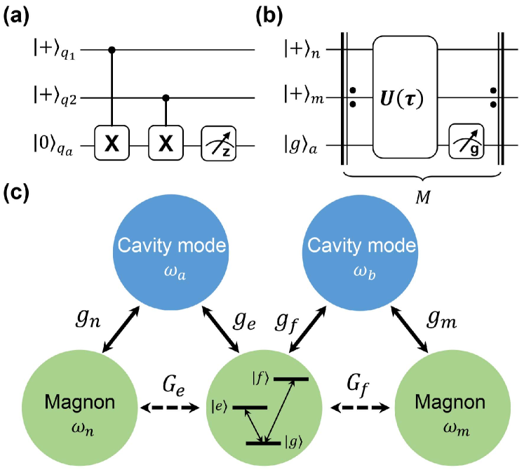
Figure 1: (a) Diagram for a typical ancillary-qubit-based parity measurement that gives rise to a qubit Bell state. (b) Diagram for our scheme to obtain a magnon Bell state by repeated rounds of free evolution and projective measurement. (c) Two magnon modes $n$ and $m$ are individually coupled to two cavity modes $a$ and $b$ with coupling strengths $g_{n}$ and $g_{m}$, respectively. The transitions $|g\rangle\leftrightarrow|e\rangle$ and $|g\rangle\leftrightarrow|f\rangle$ in a $V$-type three-level system are coupled to the cavity mode-$a$ and mode-$b$ with coupling strengths $g_{e}$ and $g_{f}$, respectively. In the dispersive regime, magnon mode-$n$ and mode-$m$ are therefore indirectly coupled to $|g\rangle\leftrightarrow|e\rangle$ and $|g\rangle\leftrightarrow|f\rangle$ with effective coupling strengths $G_{e}$ and $G_{f}$, respectively.

As shown in Fig. 1(a), a Bell state $|\Phi^{+}\rangle=(|00\rangle+|11\rangle)/\sqrt{2}$ of two transmon qubits (data qubits) could be generated by mapping the parity information to the ancillary qubit via two controlled NOT (CNOT) gates and a projective measurement on the initial state of the ancillary qubit Andersen et al. (2019). The data qubits $q_{1}$ and $q_{2}$ are prepared in a superposed state $|+\rangle|+\rangle$ with $|+\rangle\equiv(|0\rangle+|1\rangle)/\sqrt{2}$ and the ancillary qubit is prepared in $|0\rangle$. Applying two sequential CNOT gates $C(q_{i},q_{a})$, where the data qubit $q_{i}$, $i=1,2$, is the control qubit and the ancillary qubit $q_{a}$ is the target one, on the system, one can obtain an entangled state that correlates the parity information of data qubits to the ancillary qubit:

$$C(q_{1},q_{a})C(q_{2},q_{a})|++\rangle|0\rangle_{q_{a}}=|\Phi^{+}\rangle|0\rangle_{q_{a}}+|\Psi^{+}\rangle|1\rangle_{q_{a}}.$$ (1)

Here $|\Psi^{+}\rangle=(|01\rangle+|10\rangle)/\sqrt{2}$ is another Bell state with the same XX parity as $|\Phi^{+}\rangle$, i.e., $\langle\sigma_{x}\otimes\sigma_{x}\rangle=1$ for both states. Therefore, measuring the ancillary qubit and confirming it is in the initial state $|0\rangle_{q_{a}}$ heralds that the data qubits are in the target Bell state $|\Phi^{+}\rangle$.

The two CNOT gates in the circuit and the subsequent projective measurement on the ancillary qubit constitute a nonunitary operator for the data qubits. It reads,

$$\mathcal{M}=\langle 0|C(q_{1},q_{a})C(q_{2},q_{a})|0\rangle_{q_{a}}=|00\rangle\langle 00|+|11\rangle\langle 11|,$$ (2)

which is a parity-measurement operator projecting the two-qubit system into the subspace with a special parity $\langle\sigma_{z}\otimes\sigma_{z}\rangle=1$. Then the Bell-state generation could be equivalently described by applying a parity measurement on the initial state, i.e., $|\Phi^{+}\rangle=\mathcal{M}|++\rangle/P$, where $P=\langle++|\mathcal{M}|++\rangle$ is the measurement probability.

II.2 Cavity-mode-mediated magnon-atom coupling and effective parity measurement

An effective nonunitary operator similar to Eq. (2) for magnon modes can be constructed by the unitary evolution of the whole system and the projective measurement on the ancillary atom. As shown in Fig. 1(c), our model consists of two cavity modes, two magnon modes, and a $V$-type atom (superconducting qutrit). The cavity mode-$a$ is coupled to the magnon-$n$ and the atomic transition $|g\rangle\leftrightarrow|e\rangle$ and cavity mode-$b$ is coupled to the magnon-$m$ and the atomic transition $|g\rangle\leftrightarrow|f\rangle$. Practically, the interactions between magnons (atomic transitions) and cavity modes can be realized by mounting the YIG spheres near the antinode of the corresponding cavity mode Tabuchi et al. (2015); Shen et al. (2021). And the crosstalk between magnon-$n$ and cavity mode-$b$ and that between magnon-$m$ and cavity mode-$a$ are assumed to be negligible Xu et al. (2023a). The full Hamiltonian can be written as ($\hbar\equiv 1$)

$$H= \sum_{l=a,b,n,m}\omega_{l}l^{\dagger}l+\sum_{i=e,f}\omega_{i}|i\rangle\langle i|$$ (3)

$$+g_{n}(a^{\dagger}n+an^{\dagger})+g_{e}(a^{\dagger}\sigma_{eg}^{-}+a\sigma_{eg}^{+})$$

$$+g_{m}(b^{\dagger}m+bm^{\dagger})+g_{f}(b^{\dagger}\sigma_{fg}^{-}+b\sigma_{fg}^{+})$$

where $\omega_{a,b}$ are the cavity-mode frequencies, $\omega_{n,m}$ are the magnon-mode frequencies, $\omega_{e,f}$ represent frequencies of two atomic excited levels, and the atomic ground-state frequency is set to be zero. $n$ and $m$ ($a$ and $b$) are annihilation operators for magnon modes (cavity modes). $\sigma_{ig}^{-}\equiv|g\rangle\langle i|$ and $\sigma_{ig}^{+}\equiv|i\rangle\langle g|$, $i=e,f$, are atomic transition operators between excited states and the ground state. Cavity mode is coupled to magnon mode through magnetic dipole interaction and coupled to atomic transition through electric dipole interaction. $g_{n,m}$ and $g_{e,f}$ represent the interaction strengths of photon-magnon coupling and photon-atom coupling, respectively. The detunings between magnons (atomic level splitting) and the coupled cavity modes are marked with $\Delta_{n}=\omega_{n}-\omega_{a}$ and $\Delta_{m}=\omega_{m}-\omega_{b}$ ($\Delta_{e}=\omega_{e}-\omega_{a}$ and $\Delta_{f}=\omega_{f}-\omega_{b}$), respectively. In the dispersive regime that these detunings are sufficiently larger than the interaction strengths, i.e., $|g_{i}/\Delta_{i}|\ll 1$, the atom-magnon couplings could be induced by the photon-magnon coupling and the photon-atom coupling Blais et al. (2021). In this case, both magnon modes and atom are far off-resonant from the corresponding cavity modes and the cavity modes are only virtually populated. According to the Schrieffer-Wolff transformation Schrieffer and Wolff (1966), in a rotating frame with respect to

$$S =\frac{g_{n}}{\Delta_{n}}(an^{\dagger}-a^{\dagger}n)+\frac{g_{m}}{\Delta_{m}}(bm^{\dagger}-b^{\dagger}m)$$ (4)

$$+\frac{g_{e}}{\Delta_{e}}(a\sigma_{eg}^{+}-a^{\dagger}\sigma_{eg}^{-})+\frac{g_{f}}{\Delta_{f}}(b\sigma_{fg}^{+}-b^{\dagger}\sigma_{fg}^{-}),$$

an effective Hamiltonian to the second order of $g_{i}/\Delta_{i}$ can be obtained by the Baker-Campbell-Hausdorff expansion, which reads

$$\tilde{H} =\sum_{l=a,b,n,m}\tilde{\omega}_{l}l^{\dagger}l+\sum_{i=e,f}\tilde{\omega}_{i}|i\rangle\langle i|$$ (5)

$$+G_{e}(n\sigma_{eg}^{+}+n^{\dagger}\sigma_{eg}^{-})+G_{f}(m\sigma_{fg}^{+}+m^{\dagger}\sigma_{fg}^{-})$$

$$+\chi_{e}a^{\dagger}a\sigma^{z}_{eg}+\chi_{f}b^{\dagger}b\sigma^{z}_{fg}+G_{fe}(a^{\dagger}b\sigma_{fe}^{+}+ab^{\dagger}\sigma_{fe}^{-}).$$

with $\sigma^{z}_{ij}\equiv|i\rangle\langle i|-|j\rangle\langle j|$. Here the tilde frequencies

$$\tilde{\omega}_{a}=\omega_{a}-\chi_{n},\quad\tilde{\omega}_{b}=\omega_{b}-\chi_{m},\quad\tilde{\omega}_{n}=\omega_{n}+\chi_{n},$$ (6)

$$\tilde{\omega}_{m}=\omega_{m}+\chi_{m},\quad\tilde{\omega}_{e}=\omega_{e}+\chi_{e},\quad\tilde{\omega}_{f}=\omega_{f}+\chi_{f},$$

include the Lamb shifts $\chi_{i}=g_{i}^{2}/\Delta_{i}$ and the cavity-induced magnon-atom couplings take the form of

$$G_{e}=\frac{g_{e}g_{n}}{2}\left(\frac{1}{\Delta_{e}}+\frac{1}{\Delta_{n}}\right),\quad G_{f}=\frac{g_{m}g_{f}}{2}\left(\frac{1}{\Delta_{f}}+\frac{1}{\Delta_{m}}\right).$$ (7)

Note the last term in Eq. (5) is a three-body interaction about the two cavity modes and the atomic transitions $|e\rangle\leftrightarrow|f\rangle$. If the cavity modes do not significantly deviate from the initial vacuum states, i.e., $\langle a^{\dagger}a\rangle,\langle b^{\dagger}b\rangle\approx 0$, then all the three terms of the last line in Eq. (5) can be ignored and the effective Hamiltonian can be rewritten as

$$\tilde{H}^{\prime}=\tilde{\omega}_{a}a^{\dagger}a+\tilde{\omega}_{b}b^{\dagger}b+\tilde{\omega}_{n}n^{\dagger}n+\tilde{\omega}_{m}m^{\dagger}m+\tilde{\omega}_{e}|e\rangle\langle e|$$ (8)

$$+\tilde{\omega}_{f}|f\rangle\langle f|+G_{e}(n\sigma_{eg}^{+}+n^{\dagger}\sigma_{eg}^{-})+G_{f}(m\sigma_{fg}^{+}+m^{\dagger}\sigma_{fg}^{-}).$$

In the rotating frame with respect to $H_{R}=\tilde{\omega}_{a}a^{\dagger}a+\tilde{\omega}_{b}b^{\dagger}b+\tilde{\omega}_{n}(n^{\dagger}n+|e\rangle\langle e|)+\tilde{\omega}_{m}(m^{\dagger}m+|f\rangle\langle f|)$, we have a Jaynes-Cummings-like (JC) Hamiltonian:

$$H_{\rm eff}= \tilde{\Delta}_{e}|e\rangle\langle e|+\tilde{\Delta}_{f}|f\rangle\langle f|+G_{e}(n\sigma_{eg}^{+}+n^{\dagger}\sigma_{eg}^{-})$$ (9)

$$+ G_{f}(m\sigma_{fg}^{+}+m^{\dagger}\sigma_{fg}^{-}),$$

where $\tilde{\Delta}_{e}=\tilde{\omega}_{e}-\tilde{\omega}_{n}$ and $\tilde{\Delta}_{f}=\tilde{\omega}_{f}-\tilde{\omega}_{m}$. Here the effective coupling between magnons and atomic transitions are induced by exchanging virtual photons of cavity modes. In recent experiments, for a $1$ mm-diameter YIG sphere with a bare frequency $\omega_{n,m}\sim$ GHz, the dispersive coupling strengths $G_{e,f}$ are in order of MHz Xu et al. (2023a, b). In Appendix A, we provide an alternative model with a single cavity mode to achieve the same effective Hamiltonian as in Eq. (9).

An effective parity-measurement operator can be induced by an evolution-and-measurement cycle. Initially, the atom is in its ground state $|g\rangle$ and the state of two magnon modes is separable $\rho(0)=\rho_{n}(0)\otimes\rho_{m}(0)$ with a non-vanishing overlap with the target state, then the initial state of the whole system is $\rho_{\rm tot}(0)=|g\rangle\langle g|\otimes\rho(0)$. After a period of joint evolution by $U(\tau)=\exp(-iH_{\rm eff}\tau)$, the atom is measured by a projective operator $M_{g}=|g\rangle\langle g|$ and then the whole system becomes

$$\rho_{\rm tot}(\tau)=\frac{M_{g}U(\tau)\rho_{\rm tot}(0)U^{\dagger}(\tau)M_{g}}{{\rm Tr}[M_{g}U(\tau)\rho_{\rm tot}(0)U^{\dagger}(\tau)M_{g}]}.$$ (10)

According to Naimark’s dilation theorem Paulsen (2003), the projection applied on the ancillary atom induces a POVM $\mathcal{M}(\tau)[\mathcal{O}]=V_{g}(\tau)\mathcal{O}V_{g}^{\dagger}(\tau)$ on the magnon modes. Then the magnon state can be expressed as

$$\rho(\tau)=\frac{V_{g}(\tau)\rho(0)V_{g}^{\dagger}(\tau)}{P_{g}},$$ (11)

where $V(\tau)\equiv\langle g|U(\tau)|g\rangle$ is a nonunitary evolution operator acting on the magnon space and $P_{g}={\rm Tr}[V_{g}(\tau)\rho(0)V_{g}^{\dagger}(\tau)]$ is the measurement probability. Assuming that the detunings are the same $\tilde{\Delta}_{e}=\tilde{\Delta}_{f}=\Delta$, the measurement-induced evolution operator takes the form of

$$V_{g}(\tau)=e^{-i\Delta\tau/2}\sum_{n,m\geq 0}\alpha_{nm}(\tau)|nm\rangle\langle nm|$$ (12)

with coefficients

$$\alpha_{nm}(\tau)=\cos\left(\Omega_{nm}\tau\right)+i\frac{\Delta}{2\Omega_{nm}}\sin\left(\Omega_{nm}\tau\right),$$ (13)

where the Rabi frequency $\Omega_{nm}=(G_{e}^{2}n+G_{f}^{2}m+\Delta^{2}/4)^{1/2}$. Note that there is no off-diagonal element for the operator in Eq. (12) and the coefficients satisfy $|\alpha_{nm}(\tau)|\leq 1$. It means that $V_{g}(\tau)$ acts as a population-reshaping operator. Populations on the special states with $|\alpha_{nm}(\tau)|=1$ will be conserved and those on the other states with $|\alpha_{nm}(\tau)|<1$ will be gradually eliminated by repeating such evolution-and-measurement cycles.

It is straightforward to see that the ground state $|00\rangle$ always satisfies $|\alpha_{00}|=1$ due to the fact that it is decoupled from the time evolution. Then to generate a magnon Bell state $|\Phi^{+}\rangle=(|00\rangle+|11\rangle)/\sqrt{2}$, the effective coupling strengths $\Omega_{e,f}$, the detuning $\Delta$, and the free-evolution interval $\tau$ should be so engineered that $|\alpha_{11}(\tau)|=1$ with $\tau=2k\pi/\Omega_{11}$, where $k\in\mathbb{N}_{+}$. With $k=1$ or $\tau=\tau_{0}\equiv 2\pi/\Omega_{11}$, we have

$$V_{g}(\tau_{0}) =|00\rangle\langle 00|+e^{-i\phi}|11\rangle\langle 11|+e^{-i\phi}\biggl{[}\alpha_{01}(\tau_{0})|01\rangle\langle 01|$$ (14)

$$+\alpha_{10}(\tau_{0})|10\rangle\langle 10|+\sum_{n+m\geq 2}\alpha_{nm}(\tau_{0})|nm\rangle\langle nm|\biggr{]}$$

with $\phi=\pi\Delta/\Omega_{11}$. Then after $M$ rounds of free-evolution and the ground-state projection on the atom, the magnon state becomes

$$\rho(M\tau_{0}) =\underbrace{\mathcal{M}(\tau_{0})\circ\mathcal{M}(\tau_{0})\circ\cdots\circ\mathcal{M}(\tau_{0})}_{M}[\rho(0)]$$ (15)

$$=V_{g}^{M}(\tau_{0})\rho(0)V_{g}^{\dagger M}(\tau_{0})/P_{s}$$

with

$$V_{g}^{M}(\tau_{0}) =|00\rangle\langle 00|+e^{-iM\phi}|11\rangle\langle 11|$$ (16)

$$+e^{-iM\phi}\biggl{[}\alpha_{01}^{M}(\tau_{0})|01\rangle\langle 01|+\alpha_{10}^{M}(\tau_{0})|10\rangle\langle 10|$$

$$+\sum_{n+m\geq 2}\alpha_{nm}^{M}(\tau_{0})|nm\rangle\langle nm|\biggr{]}$$

and a success probability $P_{s}={\rm Tr}[V_{g}^{M}(\tau_{0})\rho(0)V_{g}^{\dagger M}(\tau_{0})]$. As measurements are repeated, the absolute value of the coefficients $|\alpha_{01}|^{M}$ and $|\alpha_{10}|^{M}$ in $V_{g}^{M}$ will exponentially vanish due to $|\alpha_{10}|,|\alpha_{01}|<1$. And the same thing occurs for $|\alpha_{02}|^{M}$ and $|\alpha_{20}|^{M}$ when $G_{e}\neq G_{f}$. Assuming that the two magnon modes are near-resonant to the relevant atomic transitions and none of them is double excited, the nonunitary evolution operator becomes an effective projection operator

$$\tilde{V}_{g}^{M}(\tau)\approx|00\rangle\langle 00|+|11\rangle\langle 11|$$ (17)

in the same form as Eq. (2). Note in our case, $|0\rangle$ and $|1\rangle$ represent the number states of magnon mode. For a resonator system, the parity operator is defined as $Q_{l}\equiv e^{i\pi l^{\dagger}l}$, which is widely used in Wigner tomography Banaszek et al. (1999); Banaszek and Wódkiewicz (1996). Then a completed parity operator of two magnon modes is written as

$$Q_{nm}=Q_{n}\otimes Q_{m}=\sum_{n,m=0}(-1)^{n+m}|nm\rangle\langle nm|,$$ (18)

where $|00\rangle$ and $|11\rangle$ are in the even parity subspace such that $\langle Q_{nm}\rangle=1$ and $|01\rangle$ and $|10\rangle$ are in the odd parity subspace such that $\langle Q_{nm}\rangle=-1$. It means that our parity-measurement operator obtained in Eq. (17) is actually a partial parity operator, projecting the magnon system into the even-parity magnon subspace.

III Preparing Bell states

Generating entanglement between macroscopic systems is an ongoing effort in quantum science, which facilitates quantum-enhanced sensing and exploration of the fundamental limits of quantum theory Thomas et al. (2021). Nevertheless, it is subject to the precise control over the system and the stability under the environmental influence Kotler et al. (2021). In this section, the parity measurement with the operator in Eq. (17) is used to generate a magnon Bell state of two YIG spheres. We first consider an “easy-mode” situation to generate a conventional Bell state where the magnon states are initialized as separable single-excitation superposed states. And then in the open-quantum-system scenario, we check the robustness of our measurement-based scheme against the environmental decoherence. To generate double- and even multiple-excitation Bell states of two magnon modes, we consider that they start from separable coherent states. It is a “hard-mode” situation for quantum control with more undesired populations over other subspaces.

III.1 Preparation Bell states from separable single-magnon superposed state

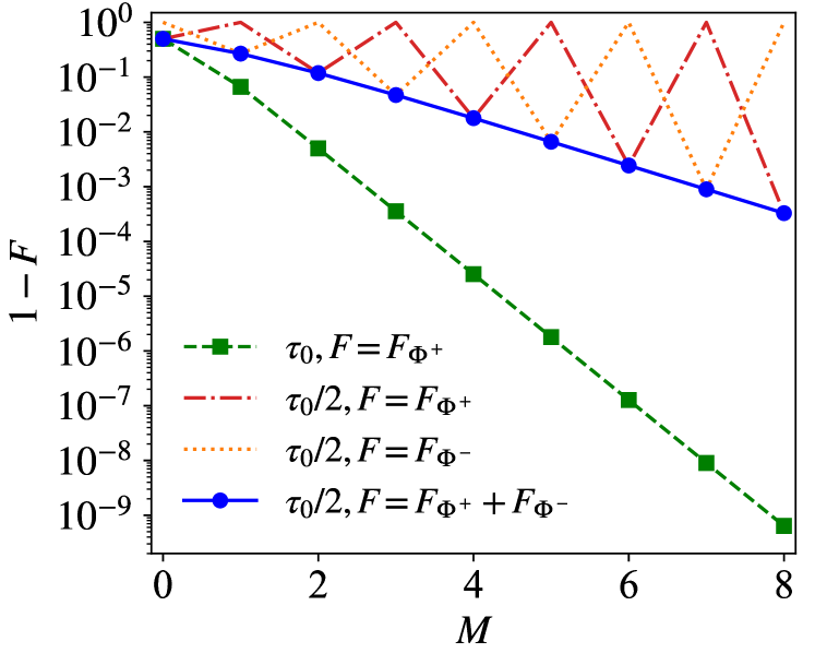
Figure 2: Infidelity of the magnon system with respect to the Bell states $|\Phi^{\pm}\rangle\equiv(|00\rangle\pm|11\rangle)/\sqrt{2}$ with a measurement interval $\tau_{0}\equiv 2\pi/\Omega_{11}$ or $\tau_{0}/2$. Magnons are assumed to be resonant with the relevant atomic transitions $\tilde{\Delta}_{e}=\tilde{\Delta}_{f}=0$ and the effective couplings are the same $G_{e}=G_{f}=10^{-3}\omega_{m}$.

We first consider preparing a magnon Bell state $|\Phi^{+}\rangle$ using the effective purity measurements in a system that the two magnon modes are initially at the same superposed state:

$$|\psi_{i}\rangle=\frac{|0\rangle+|1\rangle}{\sqrt{2}}\otimes\frac{|0\rangle+|1\rangle}{\sqrt{2}}.$$ (19)

The single-excitation superposed state in magnon system has been created in a recent experiment Xu et al. (2023a). Then the Bell state $|\Phi^{+}\rangle$ could be straightforwardly generated under several rounds of parity measurements, i.e., $|\Phi^{+}\rangle=\tilde{V}_{g}^{M}(\tau)|\psi_{i}\rangle/P_{s}$. In Fig. 2, the infidelity $1-F$ about the target Bell state with $F=F_{\Phi^{+}}$ is plotted with a green dashed line, where $F_{\Phi^{+}}\equiv\langle\Phi^{+}|\rho(t)|\Phi^{+}\rangle$. The cavity-induced coupling strengths are set the same for the best performance in fidelity. The reasons can be found in Appendix B. As the cycles of evolution and measurement are repeated, the state infidelity decreases in an exponential way. When $M=8$, it is reduced by over nine orders in magnitude from the initial state. It means that a near-to-perfect parity measurement can be induced by several projective measurements on the ancillary atom, conserving the initial population over the even parity subspace and filtering out undesired population over the odd parity subspace.

When the measurement interval is set as a half of the interval $\tau=\tau_{0}/2$ for $|\Phi^{+}\rangle$, we have $\alpha_{11}(\tau)=-1$ with $n=m=1$ due to Eq. (13). It means that the effective measurement operator in Eq. (17) becomes dependent on the parity of the measurement number $M$, i.e.,

$$\tilde{V}_{g}^{M}(\tau)\approx|00\rangle\langle 00|+(-1)^{M}|11\rangle\langle 11|.$$ (20)

We can therefore generate another Bell state $|\Phi^{-}\rangle=(|00\rangle-|11\rangle)/\sqrt{2}$ with an odd $M$, which can be described by the infidelity $1-F_{\Phi^{-}}$ in Fig. 2 (see the orange-dotted line). And when $\tau=\tau_{0}/2$ and $M$ is even, $1-F_{\Phi^{+}}$ will become vanishing. So that as the measurements are repeated, the population of the two magnon modes is swapped between $\Phi^{+}$ and $\Phi^{-}$ (see the staggered orange-dotted and red-dot-dashed lines) and gradually concentrates in the subspace of $\{|00\rangle,|11\rangle\}$ (see the blue line with markers). In other words, our scheme is capable of preparing and transferring two distinct Bell states merely by controlling the number of measurements.

The parity-measurement operator is induced by projecting the ancillary qutrit. Thus our scheme is essentially nondeterministic and one of the key metrics about the scheme efficiency is the success probability $P_{s}$. In our model, the initial population over the target entangled state provides a lower bound for the success probability, i.e., $P_{s}\geq|\langle\Phi^{+}|\psi_{i}\rangle|^{2}$. In generating $|\Phi^{\pm}\rangle$, we find the success probability after $M=8$ measurements is about $P_{s}\approx 50\%$. It is consistent with the initial condition and much larger than the probability in a previous scheme Wu et al. (2021) for generating a magnon Bell state, which is based on the magnon-induced Brillouin light scattering in an optomagnonic weak-coupling regime.

Our scheme is dramatically distinct in mechanism from those characterized by introducing or inducing nonlinear Hamiltonian or interaction Nair and Agarwal (2020); Yu et al. (2020); Zhang et al. (2019); Kong et al. (2021); Li and Zhu (2019); Wu et al. (2021); Yuan et al. (2020); Azimi Mousolou et al. (2021). For example, in Ref. Kong et al. (2021), the entanglement between two magnon modes depends on the two-magnon-mode squeezing, that is generated by the anti-JC interaction through dressing the atomic transitions by two classical fields. In contrast, our scheme depends on projecting a separable state of the system into a specific parity subspace. As for the output, squeezing induced entanglement is quantitatively evaluated by the variances of quadratures and our scheme directly gives rise to a particular entangled state, i.e., the Bell state.

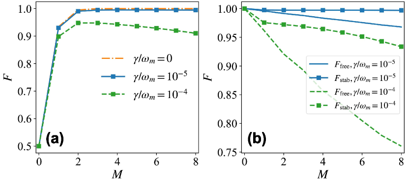
Figure 3: Fidelities of the Bell state $|\Phi^{+}\rangle$ in (a) preparation process and (b) stabilization process under various decoherence rates. The coupling strengths are set as $G_{e}=G_{f}=6\times 10^{-3}\omega_{m}$ and the measurement interval is set as $\tau=\tau_{0}$.

We consider our parity-measurement-based scheme in both state-preparation and state-stabilization processes in the presence of the environmental decoherence. In the Bell-state preparation process, the free evolution of the whole system between neighboring measurements is evaluated by the master equation

$$\dot{\rho}(t)=-i[H_{\rm eff},\rho(t)]+\gamma_{n}\mathcal{D}[n]\rho(t)+\gamma_{m}\mathcal{D}[m]\rho(t),$$ (21)

where $H_{\rm eff}$ is the effective Hamiltonian in Eq. (9) and $\mathcal{D}[A]$ represents the Lindblad superoperator

$$\mathcal{D}[A]\rho(t)\equiv A\rho(t)A^{\dagger}-\frac{1}{2}\{A^{\dagger}A,\rho(t)\}.$$ (22)

In Fig. 3(a), we plot the fidelity $F=F_{\Phi^{+}}$ in the preparation process under various decoherence rates, where the decoherence rate for each magnon mode is assumed to be the same $\gamma_{n}=\gamma_{m}=\gamma$. It is found that the target-state fidelity still rapidly increases with measurements even under decoherence. With even a large decay rate $\gamma/\omega_{m}=10^{-4}$, the final fidelity after $M=8$ measurements is over $F=0.91$, indicating that our preparation scheme is not sensitive to the environment-induced decoherence.

The projection-induced parity measurement is also capable of stabilizing the system against decoherence when the Bell-state generation is completed. In Fig. 3(b), we compare the state fidelity under the free evolution $F_{\rm free}$ and that under repeated rounds of free-evolution and projective measurements $F_{\rm stab}$. In both cases, the free evolution of system is evaluated by the master equation (21). It is found that in the absence of measurements, the fidelity $F_{\rm free}$ monotonically decreases with time due to the magnon loss. When $t=8\tau_{0}$, the fidelity will be lower than $0.77$ for $\gamma/\omega_{m}=10^{-4}$. In contrast, the decaying tendancy of the state fidelity can be significantly suppressed by the parity measurements. For $\gamma/\omega_{m}=10^{-4}$, the fidelity can be held around $F=0.93$ after $M=8$ measurements; and for $\gamma/\omega_{m}=10^{-5}$, the fidelity is maintained close to unit. These results could be understood as follows. The dominant error in generating the Bell state from the environmental decoherence is the single-magnon loss. Then the population on $|11\rangle$ tends to leak to the odd-parity subspace of $\{|10\rangle,|01\rangle\}$. Our parity measurement induced by the projection $\tilde{V}_{g}^{M}$ could avoid this error by suppressing the leakage and projecting the system into the target subspace $\{|00\rangle,|11\rangle\}$ with even parity, which thus works as a stabilizer for entanglement preparation.

III.2 Preparation Bell states from separable single-magnon coherent state

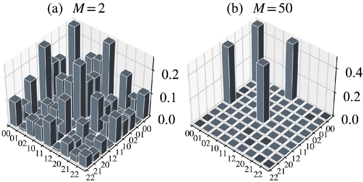
Figure 4: Tomography of the two magnon modes after (a) $M=2$ and (b) $M=50$ measurements. They starts from the same coherent state $\beta_{n}=\beta_{m}=1$. The effective couplings are set as $G_{e}=1.0\times 10^{-3}\omega_{m}$ and $G_{f}=1.2G_{e}$ and magnons are assumed to be resonant with relevant atomic transitions, i.e., $\tilde{\Delta}_{e}=\tilde{\Delta}_{f}=0$.

We consider a “hard-mode” choice of the initial states for Bell-state generation by parity measurement, which has a wide distribution over the Hilbert space. When the magnon modes are in their coherent states, the size of the subspace with different parity is clearly much larger than that of the prior initial state in Sec. III.1. Consequently, more number of measurements are expected to filter out the undesired populations than that for a single-excitation superposed state in Fig. 2. The initial state of magnon modes is written as

$$|\beta\rangle=|\beta_{n}\rangle\otimes|\beta_{m}\rangle,\quad|\beta_{l=n,m}\rangle=e^{-\frac{|\beta_{l}|^{2}}{2}}\sum_{j}\frac{\beta^{j}_{l}}{\sqrt{j}}|j\rangle.$$ (23)

The magnon coherent state could be readily realized by applying a microwave drive in resonance with the Kittel mode, which serves as a displacement operator on the vacuum state of the magnon mode $D(\beta_{i})|0\rangle$ Xu et al. (2023a). To generate the Bell state $|\Phi^{+}\rangle$, one can choose $\beta_{n}=\beta_{m}=1$ to have a significant initial overlap with the target state. We plot the state tomographies for the two magnon modes after $M=2$ and $M=50$ rounds of measurements in Fig. 4. It is found that the magnon state distribution has been dramatically reshaped only by $M=2$ measurements, where the target-state population already prevails over the others. After $M=50$ measurements, a magnon Bell state is generated with a fidelity $F\approx 0.97$.

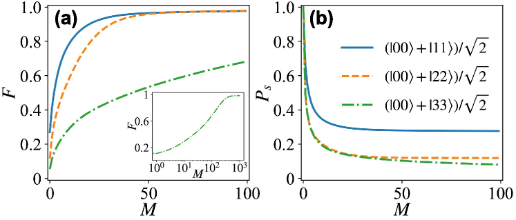
Figure 5: (a) Fidelities of the general Bell state $\langle\Phi^{+}_{N}|\rho(t)|\Phi^{+}_{N}\rangle$ and (b) Success probabilities of generating $|\Phi^{+}_{N}\rangle$ as functions of the measurement number $M$. The average excitation number of the initial coherent states for two magnon modes are set as $\beta_{n}=\beta_{m}=1,1.2,1.3$ for $N=1,2,3$, respectively. The other parameters are the same as Fig. 4.

With proper coherent states, our scheme could be generalized to prepare a multi-excitation Bell state $|\Phi^{+}_{N}\rangle=(|00\rangle+|NN\rangle)/\sqrt{2}$ that is encoded in the ground state and a high-Fock state of the magnon modes. To hold the populations on both $|00\rangle$ and $|NN\rangle$, the measurement interval $\tau$ could be chosen such that $|\alpha_{NN}(\tau)|=1$ with $\tau=2\pi/\Omega_{NN}$ and the Rabi frequency $\Omega_{NN}=(G_{e}^{2}N+G_{f}^{2}N+\Delta^{2}/4)^{1/2}$. Following a similar derivation as from Eq. (14) through Eq. (17), one can obtain an effective projection operator $|00\rangle\langle 00|+|NN\rangle\langle NN|$. We take $N=1,2,3$ in Fig. 5(a) and Fig. 5(b) to evaluate the performance of our scheme in terms of state fidelity and success probability, respectively. It is shown that a multi-excitation Bell state could be generated. The scheme becomes inefficient for a larger $N$, which results from a more dispersive distribution for the populations over a more number of undesired Fock states living between $|00\rangle$ and $|NN\rangle$. For $N=2$, the fidelity is $F=0.96$ when $M=50$ and enhanced to nearly $F=0.98$ when $M=100$. For $N=3$, $F=0.68$ when $M=100$ and $F=0.98$ when $M=10^{3}$. Figure 5(b) still supports the conclusion that the initial population over the target state serves as a lower bound for the success probability. The success probability declines as $N$ increases. The final success probabilities for $N=1,2,3$ are $P_{s}=0.28,0.12,0.08$, respectively, which are consistent with the initial fidelities shown in Fig. 5(a). Note if the magnon modes could be prepared in a superposed state of high-Fock basis $(|0\rangle+|N\rangle)\otimes(|0\rangle+|N\rangle)/2$, then the number of measurements could be much reduced as in Fig. 2.

IV Single-shot scheme

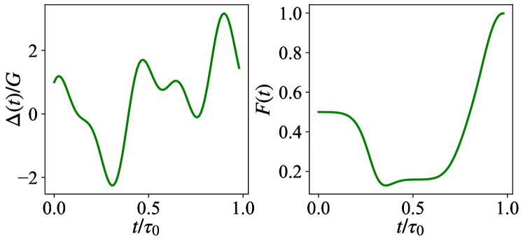
Figure 6: (a) Optimized time-dependent detuning $\Delta(t)$ found with $N_{\omega}=4$ and a total measurement interval $\tau=\tau_{0}$. (b) Bell-state fidelity evolution determined by $\Delta(t)$ in (a). The initial state is the same as Fig. (2).

According to Eqs. (16) and (17) with a fixed $\Delta$, constructing an effective parity-measurement operator demands more than one projective measurement on the ground state of the ancillary atom, that would enhance the overhead in experiments. To obtain a single-shot scheme $M=1$ for generating the Bell state, we can manipulate the detunings in Hamiltonian (9) following a similar pattern in Ref. Puebla et al. (2020) during a time interval and then perform a single-shot measurement on the ground state of the atom. In particular, the detunings in Eq. (9) are assumed to have the same magnitude $G_{e}=G_{f}=G$ and are tunable in time domain. Then the full time-dependent Hamiltonian becomes

$$H_{\rm eff}(t)=\Delta(t)(|e\rangle\langle e|+|f\rangle\langle f|)+G(n\sigma_{eg}^{+}+m\sigma_{fg}^{+}+{\rm H.c.}).$$ (24)

Aiming for the target state $|\Phi^{+}\rangle$, the function $\Delta(t)$ could be designed using the chopped-random basis approximation (CRAB) Caneva et al. (2011); Doria et al. (2011) and the Nelder-Mead search algorithm Nelder and Mead (1965). We take the evolution period $\tau_{0}$ in Eq. (14) as the total control time and fix the boundary condition $\Delta(0)/G=\Delta(\tau_{0})/G=1$. Then the task for optimizing time-dependent detuning is equivalent to finding an optimal combination of coefficients $a_{n}$ and $b_{n}$ in

$$\Delta(t)/G=1+t(\tau_{0}-t)\sum_{n=1}^{N_{\omega}}[a_{n}\cos(\omega_{n}t)+b_{n}\sin(\omega_{n}t)],$$ (25)

where $\omega_{n}=2\pi n/\tau_{0}$. Figure 6(a) demonstrates the common detuning $\Delta$ as a function of time obtained by the CRAB optimization with $N_{\omega}=4$; and Fig. 6(b) provides the corresponding time evolution of fidelity with respect to the Bell state. It is found that a magnon Bell state with a fidelity over $F=0.998$ via a near-to-perfect parity measurement of $V_{g}(\tau_{0})=|00\rangle\langle 00|+|11\rangle\langle 11|$ could be realized under such an optimized Hamiltonian engineering. It indicates that we are able to generate a macroscopic entangled state with a single-shot measurement.

V Conclusion

We propose an entangled-state generation scheme based on parity measurements over two magnon modes, which is induced by the projective measurement on the ancillary atomic system. We demonstrate that our scheme can be practiced in a hybrid magonic system, where the dispersively coupling between magnon modes and atom are induced by photon-magnon coupling and photon-atom coupling. Our scheme is dramatically distinct from those based on nonlinear interaction or squeezing Hamiltonian and the magnon Bell state can be generated from arbitrary state that has a nonvanishing population in the subspace with the desired parity. In addition to state generation, our parity measurement can stabilize the entangled state with a high fidelity against the environmental decoherence. We also propose a single-shot version for our scheme. Our work therefore enriches the quantum control based on quantum measurement and offers accessibility to generate Bell states in a macroscopic quantum system.

Appendix A Single-mode-mediated magnon-atom coupling

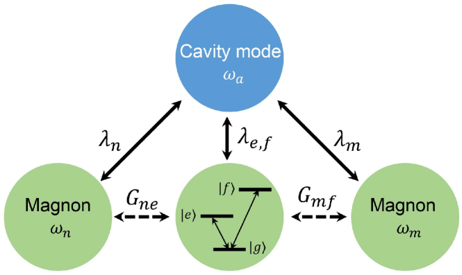
Figure 7: Two magnon modes are coupled to a common cavity mode-$a$ with coupling strengths $\lambda_{m}$ and $\lambda_{n}$, respectively. The two transitions $|g\rangle\leftrightarrow|e\rangle$ and $|g\rangle\leftrightarrow|f\rangle$ in a $V$-type three-level system are coupled to cavity mode with coupling strengths $\lambda_{e}$ and $\lambda_{f}$, respectively. As an alternative model with respect to Fig. 1(c), it also yields the same effective Hamiltonian (9) in the dispersive regime.

The model in Fig. 1(c) can be simplified to a scenario with a common cavity mode, which couples to the two atomic transitions in the same time. In this case, the full Hamiltonian becomes

$$H= \omega_{a}a^{\dagger}a+\omega_{n}n^{\dagger}n+\omega_{m}m^{\dagger}m+\omega_{e}|e\rangle\langle e|+\omega_{f}|f\rangle\langle f|$$ (26)

$$+ \lambda_{n}(a^{\dagger}n+an^{\dagger})+\lambda_{m}(a^{\dagger}m+am^{\dagger})$$

$$+ \lambda_{e}(a^{\dagger}\sigma_{eg}^{-}+a\sigma_{eg}^{+})+\lambda_{f}(a^{\dagger}\sigma_{fg}^{-}+a\sigma_{fg}^{+}),$$

where $\lambda_{n,m}$ are the coupling strengths between the cavity mode and magnon modes and $\lambda_{e,f}$ are the coupling strengths between the cavity mode and the atomic transitions. In the rotating frame with respect to

$$S= \frac{\lambda_{n}}{\Delta_{n}}(an^{\dagger}-a^{\dagger}n)+\frac{\lambda_{m}}{\Delta_{m}}(am^{\dagger}-a^{\dagger}m)$$ (27)

$$+\frac{\lambda_{e}}{\Delta_{e}}(a\sigma_{eg}^{+}-a^{\dagger}\sigma_{eg}^{-})+\frac{\lambda_{f}}{\Delta_{f}}(a\sigma_{fg}^{+}-a^{\dagger}\sigma_{fg}^{-})$$

with $\Delta_{i}\equiv\omega_{i}-\omega_{a}$, $i=n,m,e,f$, the effective Hamiltonian to the second order of $\lambda_{i}/\Delta_{i}$ reads

$$H_{\rm eff} =\tilde{\omega}_{a}a^{\dagger}a+\tilde{\omega}_{n}n^{\dagger}n+\tilde{\omega}_{m}m^{\dagger}m+\tilde{\omega}_{e}|e\rangle\langle e|+\tilde{\omega}_{f}|f\rangle\langle f|$$ (28)

$$+G_{ne}(n\sigma_{eg}^{+}+n^{\dagger}\sigma_{eg}^{-})+G_{nf}(n\sigma_{fg}^{+}+n^{\dagger}\sigma_{fg}^{-})$$

$$+G_{me}(m\sigma_{eg}^{+}+m^{\dagger}\sigma_{eg}^{-})+G_{mf}(m\sigma_{fg}^{+}+m^{\dagger}\sigma_{fg}^{-})$$

$$+G_{nm}(nm^{\dagger}+n^{\dagger}m)+G_{fe}a^{\dagger}a\sigma_{fe}^{x}$$

$$+a^{\dagger}a(\chi_{e}\sigma_{eg}^{z}+\chi_{f}\sigma_{fg}^{z}),$$

where

$$\tilde{\omega}_{a}=\omega_{a}-\chi_{n}-\chi_{m},\quad\tilde{\omega}_{n}=\omega_{n}+\chi_{n},$$ (29)

$$\tilde{\omega}_{m}=\omega_{m}+\chi_{m},\quad\tilde{\omega}_{e}=\omega_{e}+\chi_{e},\quad\tilde{\omega}_{f}=\omega_{f}+\chi_{f}$$

with the Lamb shifts $\chi_{i}=\lambda_{i}^{2}/\Delta_{i}$, $\sigma_{ij}^{x}\equiv|i\rangle\langle j|+|j\rangle\langle i|$ and $\sigma_{ij}^{z}\equiv|i\rangle\langle i|-|j\rangle\langle j|$. The coupling strengths induced by the cavity mode could be expressed as

$$G_{ij}=\frac{\lambda_{i}\lambda_{j}}{2}\left(\frac{1}{\Delta_{i}}+\frac{1}{\Delta_{j}}\right).$$ (30)

In comparison to the dispersively induced effective Hamiltonian (5) for the two-cavity-mode situation, cross interactions emerge in the effective Hamiltonian (28) for the single-cavity-mode situation. They include the interaction $G_{nf}$ between magnon-$n$ and transition $|g\rangle\leftrightarrow|f\rangle$, the interaction $G_{me}$ between magnon-$m$ and transition $|g\rangle\leftrightarrow|e\rangle$, and the interaction $G_{fe}$ between two excited levels in atom. However, these terms could be cancelled under the detuning-match condition:

$$\Delta_{n}=\Delta_{e}=-\Delta_{m}=-\Delta_{f}.$$ (31)

Together with the vacuum-state assumption $\langle a^{\dagger}a\rangle\approx 0$, the effective Hamiltonian becomes

$$H_{\rm eff} =\tilde{\omega}_{a}a^{\dagger}a+\tilde{\omega}_{n}n^{\dagger}n+\tilde{\omega}_{m}m^{\dagger}m+\tilde{\omega}_{e}|e\rangle\langle e|+\tilde{\omega}_{f}|f\rangle\langle f|$$ (32)

$$+G_{ne}(n\sigma_{eg}^{+}+n^{\dagger}\sigma_{eg}^{-})+G_{mf}(m\sigma_{fg}^{+}+m^{\dagger}\sigma_{fg}^{-}).$$

In the rotating frame with respect to $H_{R}=\tilde{\omega}_{a}a^{\dagger}a+\tilde{\omega}_{n}(n^{\dagger}n+|e\rangle\langle e|)+\tilde{\omega}_{m}(m^{\dagger}m+|f\rangle\langle f|)$, we have exactly the same form as Hamiltonian in Eq. (9):

$$H^{\prime}_{eff}= \tilde{\Delta}_{e}|e\rangle\langle e|+\tilde{\Delta}_{f}|f\rangle\langle f|+G_{ne}(n\sigma_{eg}^{+}+n^{\dagger}\sigma_{eg}^{-})$$ (33)

$$+G_{mf}(m\sigma_{fg}^{+}+m^{\dagger}\sigma_{fg}^{-})$$

with $\tilde{\Delta}_{e}=\tilde{\omega}_{e}-\tilde{\omega}_{n}$ and $\tilde{\Delta}_{f}=\tilde{\omega}_{f}-\tilde{\omega}_{m}$.

Appendix B Coupling-ratio optimization in Bell state generation

Figure 8: Fidelities of the Bell state $|\Phi^{+}\rangle$ under a single parity measurement as a function of the coupling-strength ratio $G_{e}/G_{f}$ with and without the second-order approximation in Eq. (37). The other parameters are the same as those in Fig. 2.

This appendix contributes to estimating the effect of the ratio $G_{e}/G_{f}$ about magnons-atom interaction on Bell state generation. For simplicity, we consider the same initial condition in Fig. 2. And in the near-resonant regime, the measurement-induced evolution operator for the two magnon modes in Eq. (14) can be written as

$$V_{g}(\tau_{0})\approx|00\rangle\langle 00|+|11\rangle\langle 11|+\alpha_{01}|01\rangle\langle 01|+\alpha_{10}|10\rangle\langle 10|$$ (34)

with

$$\alpha_{01}=\cos\frac{2\pi G_{f}}{\sqrt{G_{e}^{2}+G_{f}^{2}}},\quad\alpha_{10}=\cos\frac{2\pi G_{e}}{\sqrt{G_{e}^{2}+G_{f}^{2}}}$$ (35)

where the measurement interval is fixed as $\tau=\tau_{0}=2\pi/(G_{e}^{2}+G_{f}^{2})^{1/2}$. Then after a single round of evolution and measurement, the fidelity of the Bell state can be written as

$$F=\frac{|\langle\Phi^{+}|V_{g}(\tau)|\psi_{i}\rangle|^{2}}{{\rm Tr}[V_{g}(\tau)|\psi_{i}\rangle\langle\psi_{i}|V_{g}^{\dagger}(\tau)]}=\frac{2}{2+\alpha_{01}^{2}(\tau)+\alpha_{10}^{2}(\tau)}.$$ (36)

Accordingly, the non-zero coefficients $\alpha_{10}(\tau)$ and $\alpha_{01}(\tau)$ result in an imperfect parity measurement by reducing the final Bell-state fidelity. When $G_{e}\approx G_{f}$, both coefficients can be expanded around the coupling ratio $\xi\equiv G_{f}/G_{e}=1$. To the order of $\mathcal{O}[(\xi-1)^{2}]$, we have

$$\alpha_{01}(\tau)\approx\tilde{\alpha}_{01}(\tau)=\cos(\sqrt{2}\pi)-\frac{\pi}{\sqrt{2}}\sin(\sqrt{2}\pi)(\xi-1)$$ (37)

$$\alpha_{10}(\tau)\approx\tilde{\alpha}_{10}(\tau)=\cos(\sqrt{2}\pi)+\frac{\pi}{\sqrt{2}}\sin(\sqrt{2}\pi)(\xi-1).$$

Then the denominator in Eq. (36) depends on

$$\alpha_{01}^{2}+\alpha_{10}^{2}=\cos^{2}(\sqrt{2}\pi)+\frac{\pi^{2}}{2}\sin^{2}(\sqrt{2}\pi)(\xi-1)^{2}.$$ (38)

It is straightforward to see that the Bell-state generation is optimized when $\xi=1$, i.e., $G_{e}/G_{f}=1$. In Fig. 8, the Bell-state fidelities are plotted with the coefficients in Eq. (35) and those in Eq. (37). It is shown that Eq. (37) is a good approximation to Eq. (35).

References

- Misra and Sudarshan (1977) B. Misra and E. C. G. Sudarshan, The zeno’s paradox in quantum theory, J. Math. Phys. 18, 756 (1977).
- Aharonov and Vardi (1980) Y. Aharonov and M. Vardi, Meaning of an individual “feynman path”, Phys. Rev. D 21, 2235 (1980).
- Altenmüller and Schenzle (1993) T. P. Altenmüller and A. Schenzle, Dynamics by measurement: Aharonov’s inverse quantum zeno effect, Phys. Rev. A 48, 70 (1993).
- Roa et al. (2006) L. Roa, A. Delgado, M. L. Ladrón de Guevara, and A. B. Klimov, Measurement-driven quantum evolution, Phys. Rev. A 73, 012322 (2006).
- Pechen et al. (2006) A. Pechen, N. Il’in, F. Shuang, and H. Rabitz, Quantum control by von neumann measurements, Phys. Rev. A 74, 052102 (2006).
- Paulsen (2003) V. Paulsen, Completely Bounded Maps and Operator Algebras (Cambridge University Press, Cambridge, 2003).
- Li et al. (2011) Y. Li, L.-A. Wu, Y.-D. Wang, and L.-P. Yang, Nondeterministic ultrafast ground-state cooling of a mechanical resonator, Phys. Rev. B 84, 094502 (2011).
- Buffoni et al. (2019) L. Buffoni, A. Solfanelli, P. Verrucchi, A. Cuccoli, and M. Campisi, Quantum measurement cooling, Phys. Rev. Lett. 122, 070603 (2019).
- Yan and Jing (2021) J.-S. Yan and J. Jing, External-level assisted cooling by measurement, Phys. Rev. A 104, 063105 (2021).
- Xu et al. (2014) J.-S. Xu, M.-H. Yung, X.-Y. Xu, S. Boixo, Z.-W. Zhou, C.-F. Li, A. Aspuru-Guzik, and G.-C. Guo, Demon-like algorithmic quantum cooling and its realization with quantum optics, Nat. Photonics 8, 113 (2014).
- Rao et al. (2016) D. D. B. Rao, S. A. Momenzadeh, and J. Wrachtrup, Heralded control of mechanical motion by single spins, Phys. Rev. Lett. 117, 077203 (2016).
- Seah et al. (2021) S. Seah, M. Perarnau-Llobet, G. Haack, N. Brunner, and S. Nimmrichter, Quantum speed-up in collisional battery charging, Phys. Rev. Lett. 127, 100601 (2021).
- Yan and Jing (2023) J.-S. Yan and J. Jing, Charging by quantum measurement, Phys. Rev. Appl. 19, 064069 (2023).
- Terhal (2015) B. M. Terhal, Quantum error correction for quantum memories, Rev. Mod. Phys. 87, 307 (2015).
- Gottesman et al. (2001) D. Gottesman, A. Kitaev, and J. Preskill, Encoding a qubit in an oscillator, Phys. Rev. A 64, 012310 (2001).
- Saira et al. (2014) O.-P. Saira, J. P. Groen, J. Cramer, M. Meretska, G. de Lange, and L. DiCarlo, Entanglement genesis by ancilla-based parity measurement in 2d circuit QED, Phys. Rev. Lett. 112, 070502 (2014).
- Ristè et al. (2013) D. Ristè, M. Dukalski, C. A. Watson, G. de Lange, M. J. Tiggelman, Y. M. Blanter, K. W. Lehnert, R. N. Schouten, and L. DiCarlo, Deterministic entanglement of superconducting qubits by parity measurement and feedback, Nature 502, 350 (2013).
- Andersen et al. (2019) C. K. Andersen, A. Remm, S. Lazar, S. Krinner, J. Heinsoo, J.-C. Besse, M. Gabureac, A. Wallraff, and C. Eichler, Entanglement stabilization using ancilla-based parity detection and real-time feedback in superconducting circuits, npj Quantum Inf. 5, 69 (2019).
- Blumenthal et al. (2022) E. Blumenthal, C. Mor, A. A. Diringer, L. S. Martin, P. Lewalle, D. Burgarth, K. B. Whaley, and S. Hacohen-Gourgy, Demonstration of universal control between non-interacting qubits using the quantum zeno effect, npj Quantum Inf. 8, 88 (2022).
- Banaszek et al. (1999) K. Banaszek, C. Radzewicz, K. Wódkiewicz, and J. S. Krasiński, Direct measurement of the wigner function by photon counting, Phys. Rev. A 60, 674 (1999).
- Banaszek and Wódkiewicz (1996) K. Banaszek and K. Wódkiewicz, Direct probing of quantum phase space by photon counting, Phys. Rev. Lett. 76, 4344 (1996).
- Besse et al. (2020) J.-C. Besse, S. Gasparinetti, M. C. Collodo, T. Walter, A. Remm, J. Krause, C. Eichler, and A. Wallraff, Parity detection of propagating microwave fields, Phys. Rev. X 10, 011046 (2020).
- Banaszek and Wódkiewicz (1998) K. Banaszek and K. Wódkiewicz, Nonlocality of the einstein-podolsky-rosen state in the wigner representation, Phys. Rev. A 58, 4345 (1998).
- Lachance-Quirion et al. (2019) D. Lachance-Quirion, Y. Tabuchi, A. Gloppe, K. Usami, and Y. Nakamura, Hybrid quantum systems based on magnonics, Appl. Phys. Express 12, 070101 (2019).
- Yuan et al. (2022) H. Yuan, Y. Cao, A. Kamra, R. A. Duine, and P. Yan, Quantum magnonics: When magnon spintronics meets quantum information science, Phys. Rep. 965, 1 (2022).
- Zare Rameshti et al. (2022) B. Zare Rameshti, S. Viola Kusminskiy, J. A. Haigh, K. Usami, D. Lachance-Quirion, Y. Nakamura, C.-M. Hu, H. X. Tang, G. E. Bauer, and Y. M. Blanter, Cavity magnonics, Phys. Rep. 979, 1 (2022).
- Huebl et al. (2013) H. Huebl, C. W. Zollitsch, J. Lotze, F. Hocke, M. Greifenstein, A. Marx, R. Gross, and S. T. B. Goennenwein, High cooperativity in coupled microwave resonator ferrimagnetic insulator hybrids, Phys. Rev. Lett. 111, 127003 (2013).
- Tabuchi et al. (2014) Y. Tabuchi, S. Ishino, T. Ishikawa, R. Yamazaki, K. Usami, and Y. Nakamura, Hybridizing ferromagnetic magnons and microwave photons in the quantum limit, Phys. Rev. Lett. 113, 083603 (2014).
- Zhang et al. (2014) X. Zhang, C.-L. Zou, L. Jiang, and H. X. Tang, Strongly coupled magnons and cavity microwave photons, Phys. Rev. Lett. 113, 156401 (2014).
- Bai et al. (2015) L. Bai, M. Harder, Y. P. Chen, X. Fan, J. Q. Xiao, and C.-M. Hu, Spin pumping in electrodynamically coupled magnon-photon systems, Phys. Rev. Lett. 114, 227201 (2015).
- Zhang et al. (2016) X. Zhang, C.-L. Zou, L. Jiang, and H. X. Tang, Cavity magnomechanics, Sci. Adv. 2, e1501286 (2016).
- Potts et al. (2021) C. A. Potts, E. Varga, V. A. S. V. Bittencourt, S. V. Kusminskiy, and J. P. Davis, Dynamical backaction magnomechanics, Phys. Rev. X 11, 031053 (2021).
- Tabuchi et al. (2015) Y. Tabuchi, S. Ishino, A. Noguchi, T. Ishikawa, R. Yamazaki, K. Usami, and Y. Nakamura, Coherent coupling between a ferromagnetic magnon and a superconducting qubit, Science 349, 405 (2015).
- Tabuchi et al. (2016) Y. Tabuchi, S. Ishino, A. Noguchi, T. Ishikawa, R. Yamazaki, K. Usami, and Y. Nakamura, Quantum magnonics: The magnon meets the superconducting qubit, C. R. Phys. 17, 729 (2016).
- Lachance-Quirion et al. (2017) D. Lachance-Quirion, Y. Tabuchi, S. Ishino, A. Noguchi, T. Ishikawa, R. Yamazaki, and Y. Nakamura, Resolving quanta of collective spin excitations in a millimeter-sized ferromagnet, Sci. Adv. 3, e1603150 (2017).
- Nair and Agarwal (2020) J. M. P. Nair and G. S. Agarwal, Deterministic quantum entanglement between macroscopic ferrite samples, Appl. Phys. Lett. 117, 084001 (2020).
- Yu et al. (2020) M. Yu, S.-Y. Zhu, and J. Li, Macroscopic entanglement of two magnon modes via quantum correlated microwave fields, J. Phys. B: At., Mol., Opt. Phys. 53, 065402 (2020).
- Zhang et al. (2019) Z. Zhang, M. O. Scully, and G. S. Agarwal, Quantum entanglement between two magnon modes via kerr nonlinearity driven far from equilibrium, Phys. Rev. Res. 1, 023021 (2019).
- Li and Zhu (2019) J. Li and S.-Y. Zhu, Entangling two magnon modes via magnetostrictive interaction, New J. Phys. 21, 085001 (2019).
- Wu et al. (2021) W.-J. Wu, Y.-P. Wang, J.-Z. Wu, J. Li, and J. Q. You, Remote magnon entanglement between two massive ferrimagnetic spheres via cavity optomagnonics, Phys. Rev. A 104, 023711 (2021).
- Yuan et al. (2020) H. Y. Yuan, S. Zheng, Z. Ficek, Q. Y. He, and M.-H. Yung, Enhancement of magnon-magnon entanglement inside a cavity, Phys. Rev. B 101, 014419 (2020).
- Azimi Mousolou et al. (2021) V. Azimi Mousolou, Y. Liu, A. Bergman, A. Delin, O. Eriksson, M. Pereiro, D. Thonig, and E. Sjöqvist, Magnon-magnon entanglement and its quantification via a microwave cavity, Phys. Rev. B 104, 224302 (2021).
- Daiss et al. (2019) S. Daiss, S. Welte, B. Hacker, L. Li, and G. Rempe, Single-photon distillation via a photonic parity measurement using cavity QED, Phys. Rev. Lett. 122, 133603 (2019).
- Shen et al. (2021) R.-C. Shen, Y.-P. Wang, J. Li, S.-Y. Zhu, G. S. Agarwal, and J. Q. You, Long-time memory and ternary logic gate using a multistable cavity magnonic system, Phys. Rev. Lett. 127, 183202 (2021).
- Xu et al. (2023a) D. Xu, X.-K. Gu, H.-K. Li, Y.-C. Weng, Y.-P. Wang, J. Li, H. Wang, S.-Y. Zhu, and J. Q. You, Quantum control of a single magnon in a macroscopic spin system, Phys. Rev. Lett. 130, 193603 (2023a).
- Blais et al. (2021) A. Blais, A. L. Grimsmo, S. M. Girvin, and A. Wallraff, Circuit quantum electrodynamics, Rev. Mod. Phys. 93, 025005 (2021).
- Schrieffer and Wolff (1966) J. R. Schrieffer and P. A. Wolff, Relation between the anderson and kondo hamiltonians, Phys. Rev. 149, 491 (1966).
- Xu et al. (2023b) D. Xu, X.-K. Gu, Y.-C. Weng, H.-K. Li, Y.-P. Wang, S.-Y. Zhu, and J. Q. You, Deterministic generation and tomography of a macroscopic bell state between a millimeter-sized spin system and a superconducting qubit, arXiv , 2306.09677 (2023b).
- Thomas et al. (2021) R. A. Thomas, M. Parniak, C. Østfeldt, C. B. Møller, C. Bærentsen, Y. Tsaturyan, A. Schliesser, J. Appel, E. Zeuthen, and E. S. Polzik, Entanglement between distant macroscopic mechanical and spin systems, Nat. Phys. 17, 228 (2021).
- Kotler et al. (2021) S. Kotler, G. A. Peterson, E. Shojaee, F. Lecocq, K. Cicak, A. Kwiatkowski, S. Geller, S. Glancy, E. Knill, R. W. Simmonds, J. Aumentado, and J. D. Teufel, Direct observation of deterministic macroscopic entanglement, Science 372, 622 (2021).
- Kong et al. (2021) D. Kong, X. Hu, L. Hu, and J. Xu, Magnon-atom interaction via dispersive cavities: Magnon entanglement, Phys. Rev. B 103, 224416 (2021).
- Puebla et al. (2020) R. Puebla, O. Abah, and M. Paternostro, Measurement-based cooling of a nonlinear mechanical resonator, Phys. Rev. B 101, 245410 (2020).
- Caneva et al. (2011) T. Caneva, T. Calarco, and S. Montangero, Chopped random-basis quantum optimization, Phys. Rev. A 84, 022326 (2011).
- Doria et al. (2011) P. Doria, T. Calarco, and S. Montangero, Optimal control technique for many-body quantum dynamics, Phys. Rev. Lett. 106, 190501 (2011).
- Nelder and Mead (1965) J. A. Nelder and R. Mead, A Simplex Method for Function Minimization, Comput. J. 7, 308 (1965).