Differentiable Tree Search in
Latent State Space

Abstract

In decision-making problems with limited training data, policy functions approximated using deep neural networks often exhibit suboptimal performance. An alternative approach involves learning a world model from the limited data and determining actions through online search. However, the performance is adversely affected by compounding errors arising from inaccuracies in the learnt world model. While methods like TreeQN have attempted to address these inaccuracies by incorporating algorithmic structural biases into their architectures, the biases they introduce are often weak and insufficient for complex decision-making tasks. In this work, we introduce Differentiable Tree Search (DTS), a novel neural network architecture that significantly strengthens the inductive bias by embedding the algorithmic structure of a best-first online search algorithm. DTS employs a learnt world model to conduct a fully differentiable online search in latent state space. The world model is jointly optimised with the search algorithm, enabling the learning of a robust world model and mitigating the effect of model inaccuracies. We address potential Q-function discontinuities arising from naive incorporation of best-first search by adopting a stochastic tree expansion policy, formulating search tree expansion as a decision-making task, and introducing an effective variance reduction technique for the gradient computation. We evaluate DTS in an offline-RL setting with a limited training data scenario on Procgen games and grid navigation task, and demonstrate that DTS outperforms popular model-free and model-based baselines.

1 Introduction

Deep Reinforcement Learning (DRL) has advanced significantly in addressing complex sequential decision-making problems, largely due to advances in Deep Neural Networks (DNN) (Silver et al., 2017b; Berner et al., 2019; Vinyals et al., 2019). The superior representational capacity of DNNs enables an agent to learn a direct mapping from observations to actions through a policy (Mnih et al., 2016; Schulman et al., 2015b; 2017; Cobbe et al., 2021) or Q-value function (Mnih et al., 2013; Wang et al., 2016; van Hasselt et al., 2016; Hessel et al., 2018; Badia et al., 2020). However, DRL has high sample complexity and weak generalisation capability that limits its wider application in complex real-world settings, especially when a limited training data is available.

Model-based Reinforcement Learning (MBRL) approaches (Kaiser et al., 2020; Hafner et al., 2020; Ha & Schmidhuber, 2018) address this by learning world models from limited environment interactions and subsequently using these models for online search (Hafner et al., 2020; 2019) or policy learning (Kaiser et al., 2020). Although MBRL is effective for problems where learning the world model is simpler than learning the policy, its efficacy diminishes for complex, long-horizon problems due to accumulated errors arising from inevitable inaccuracies in the learnt world model.

Some recent attempts (Racanière et al., 2017; Silver et al., 2017a; Lee et al., 2018; Tamar et al., 2016; Farquhar et al., 2018; Guez et al., 2019) have tried to improve the sample efficiency and generalisation capabilities of DNN models by incorporating algorithmic structural biases into the network architecture. These inductive biases restrict the class of functions a model can learn by leveraging domain-specific knowledge, reducing the likelihood of the model overfitting to the training data and learning a model incompatible with the domain knowledge. Despite their potential, the weaker structural biases imposed by current methods limits the extent of their benefits.

A notable recent work, TreeQN (Farquhar et al., 2018), combines look-ahead tree search with deep neural networks. It dynamically constructs a computation graph by fully expanding the search tree up to a predefined depth $d$ using a learnt world model and computing the Q-values at the root node by recursively applying Bellman equation on the tree nodes. The whole structure is trained end-to-end and enables learning a robust world model that is helpful in the look-ahead tree search. Consequently, TreeQN outperforms conventional neural network architectures on multiple Atari games. However, the size of the full search tree grows exponentially in the depth, which computationally limits the TreeQN to perform only a shallow search. This issue limits TreeQN’s ability to fully exploit the domain knowledge of advanced online search algorithms that can handle problems requiring much deeper search.

In this paper, we extend the foundational concepts of TreeQN, and propose Differentiable Tree Search (DTS), a novel neural network architecture that addresses these limitations by embedding the algorithmic structure of a best-first search algorithm into the network architecture. DTS has a modular design and consists several learnable submodules that dynamically combine to construct a computation graph by following a best-first search algorithm. As the computation graph is end-to-end differentiable, we jointly optimise the search submodules and the learnt world model using gradient-based optimisation. Joint optimisation enables learning a robust world model that is useful in the online search and optimises search submodules to account for the inaccuracies in the learnt world model.

However, a naive incorporation of a best-first search algorithm in the network design might lead to a Q-function which is discontinuous in the network’s parameter space. This is because a small change in parameters might result in a different sampled tree and might bring large change in output Q-value. Consequently, the Q-function might be difficult to optimise as gradient-based optimisation techniques generally requires a continuous function for optimisation. To address this, we propose employing a stochastic tree expansion policy and optimising the expected Q-value at the root node, ensuring the continuity of Q-function in the network’s parameter space. Furthermore, we propose formulating the search tree expansion as a decision-making task with the goal of progressively minimising the prediction error in the Q-value, and refining the tree expansion policy via REINFORCE (Williams, 1992). The REINFORCE algorithm has high variance in its gradient estimate and we further propose the use of the telescoping sum trick used in Guez et al. (2018) as an effective variance reduction method.

We compare DTS against popular baselines that include model-free Q-network, to assess the impact of incorporating algorithmic structural biases into the network architecture; TreeQN, to assess the benefits of incorporating a better online search algorithm capable of performing a deeper search within the same computational budget; and an online search with a learnt world model, to evaluate the advantages of jointly learning the model with the search algorithm. We evaluate these methods on deterministic decision making problems, including Procgen games (Cobbe et al., 2020) and a small-scale 2D grid navigation problem, to examine their generalisation capabilities. Empirical evaluations demonstrate that DTS outperforms the baselines in both Procgen and navigation tasks.

2 Related Works

In recent years, Reinforcement Learning (RL) has undergone remarkable advancements, notably due to the integration of Deep Neural Networks (DNNs) in domains such as Q-learning (Mnih et al., 2013; Wang et al., 2016; van Hasselt et al., 2016; Hessel et al., 2018; Espeholt et al., 2018; Badia et al., 2020) and policy learning (Williams, 1992; Schulman et al., 2015b; 2017; Mnih et al., 2016). Moreover, model-based RL has been significantly enriched by a series of innovative works (Deisenroth & Rasmussen, 2011; Nagabandi et al., 2018; Chua et al., 2018) that learn World Models (Ha & Schmidhuber, 2018) from pixels and subsequently utilise them for planning (Hafner et al., 2020; 2019; Schrittwieser et al., 2020) and policy learning (Kaiser et al., 2020).

An intriguing dimension of research in RL seeks to merge learning and planning paradigms. AlphaZero (Silver et al., 2017b) utilises DNNs as heuristics with Monte Carlo Tree Search (MCTS). On the other hand, use of inductive biases (Hessel et al., 2019) has been explored for their impact on policy learning. Recent works like Value Iteration Network (VIN) (Tamar et al., 2016) represents value iteration algorithm in gridworld domains using a convolutional neural network. Similarly, Gated Path Planning Network (Lee et al., 2018) replaces convolution blocks in VIN with LSTM blocks to address vanishing or exploding gradient issue. Further, Neural A* Search (Yonetani et al., 2021) embeds A* algorithm into network architecture and learns a cost function from a gridworld map. Alternatively, Neural Admissible Relaxation (NEAR) (Shah et al., 2020) learns an approximately admissible heuristics for A* algorithm. Works like Predictron (Silver et al., 2017a) and Value Prediction Network (Oh et al., 2017) employs a learnt world model to simulate rollouts and accumulate internal rewards in an end-to-end framework. Extending this paradigm, Imagination-based Planner (IBP) (Pascanu et al., 2017) utilises an unstructured memory representation to collate information from the internal rollouts. Alternatively, MCTSnets (Guez et al., 2018) embeds the structure of Monte Carlo Tree Search (MCTS) in the network architecture and steers the search using parameterised memory embeddings stored in a tree structure. However, Guez et al. (2019) suggests that recurrent neural networks could display certain planning properties without requiring a specific algorithmic structure in network architecture.

Our work on DTS draws inspiration from these recent contributions, notably TreeQN (Farquhar et al., 2018). TreeQN employs a full tree expansion up to a fixed depth, followed by recursive updates to the value estimate of tree nodes in order to predict the Q-value at the input state. However, TreeQN’s full tree expansion is exponential in the depth, rendering it computationally expensive for tackling complex planning problems that necessitate deeper search. DTS addresses this issue by incorporating a more advanced online search algorithm that emphasises expansion in promising areas of the search tree.

3 Differentiable Tree Search

Differentiable Tree Search (DTS) is a neural network architecture that incorporates the structural bias of a best-first search algorithm into the network design. Moreover, DTS employs a learnt world model to eliminate the dependency on availability of a world simulator. The learnt world model is jointly optimised with the online search algorithm using gradient-based optimisation techniques, such that the learnt world model, although imperfect, is useful for the online search, and search submodules are robust against errors in the world model.

3.1 Learnable Submodules

DTS is built upon several learnable submodules, which are employed as subroutines in alignment with a best-first search algorithm to dynamically construct the computation graph. Encoder Module ($\mathcal{E}_{\theta}$) encodes an actual state $s_{t}$ into a latent state representation $h_{t}$, where $h_{t}=\mathcal{E}_{\theta}(s_{t})$, and enables conduction of online search in a latent space. Transition Module ($\mathcal{T}_{\theta}$) approximates the transition function of the underlying model. It uses latent state $h_{t}$ and action $a_{t}$ as inputs to predict latent state $h_{t+1}$ of the next state, i.e. $h_{t+1}=\mathcal{T}_{\theta}(h_{t},a_{t})$. Reward Module ($\mathcal{R}_{\theta}$) approximates the reward function of the underlying model. Similar to the transition module, it takes latent state $h_{t}$ and action $a_{t}$ as inputs, and predicts the corresponding reward $r_{t}$ for the transition, i.e. $r_{t}=\mathcal{R}_{\theta}(h_{t},a_{t})$. Value Module ($\mathcal{V}_{\theta}$) approximates the value function of the underlying model by mapping latent state $h_{t}$ to its estimated state value $\mathcal{V}_{\theta}(h_{t})$.

By breaking the network into these submodules and reusing them, the total number of learnable parameters is effectively reduced, helping to prevent overfitting to an arbitrary function that may align with the given training data.

3.2 Online Search in Latent Space

The search begins by encoding the input state $s_{0}$ into its latent state $h_{0}$ at the root node. Following this, Differentiable Tree Search proceeds in two stages. In the expansion phase, DTS iteratively expands the search tree from the input state for a fixed number of node expansions (each expansion is referred to as search trial). The expansion phase is followed by the backup phase, where the Q-values at the root node are recursively computed by applying the Bellman equation on the expanded tree nodes. Each node in the tree represents a latent state reachable from the root node, whereas each branch represents an action taken at the tree node. A set of candidate nodes, $O$, is maintained during the expansion phase, representing the tree nodes eligible for further expansion. The pseudo-code of DTS is presented in Algorithm 1 in the appendix.

In the Expansion phase, each trial begins by evaluating the total path value, $\bar{V}(N)$, of the candidate nodes. The total path value is the cumulative sum of rewards from the root node to a particular leaf node $N$, in addition to the value of the leaf node predicted by the value module, $\mathcal{V}_{\theta}(h_{N})$, i.e.

$$\bar{V}(N)=\mathcal{R}_{\theta}(h_{0},a_{0})+...+\mathcal{R}_{\theta}(h_{N-1},a_{N-1})+\mathcal{V}_{\theta}(h_{N})$$ (1)

The node $N^{*}$ with the highest total path value is selected for expansion in the deterministic search version; for differentiable search, a node is sampled from the candidates using a distribution constructed with the softmax of the path values of the candidates. This expansion is carried out by simulating every action on the node $N^{*}$ using the Transition module, $\mathcal{T}_{\theta}$. Simultaneously, the associated reward, $\mathcal{R}_{\theta}(h_{N^{*}},a)$, is derived. The resulting latent states are incorporated into the tree as children of the node $N^{*}$. Additionally, they are added to the candidate set $O$ to be considered for subsequent expansions, while $N^{*}$ is excluded from the set. This can be represented as:

$$O\leftarrow O\cup{h_{a}|\ h_{a}=\mathcal{T}_{\theta}(h_{N^{*}},a);\forall a\in A}-N^{*}$$

The expansion phase is followed by the Backup phase. In this phase, value of all the tree nodes is recursively updated using the Bellman equation as follows:

$$Q(N,a) =\mathcal{R}_{\theta}(h_{N},a)+V\big{(}\mathcal{T}_{\theta}(h_{N},a)\big{)}$$

$$V(N) =\begin{cases}\mathcal{V}_{\theta}(h_{N}),&\text{N is a leaf node}\\ \max_{a}Q(N,a),&\text{otherwise}\end{cases}$$

After the Backup phase, the Q-values at the root node are returned as the final output of the online search.

Throughout the Expansion and Backup phases, a dynamic computation graph is constructed where the output Q-values depend on the submodules, namely Encoder, Transition, Reward, and Value modules. During training, the output Q-values are evaluated by a loss function. Gradient-based optimisers such as Stochastic Gradient Descent (SGD) backpropagates the gradient of this loss through the entire computation graph, and updates the parameters of each submodule in an end-to-end process.

3.3 Discontinuity of Q-function

For the effective optimisation of a neural network’s parameters using gradient descent, it is desirable for the network’s output to be continuous in the parameter space. We first show that a network which is constructed from a full tree expansion to a fixed depth $d$, as used in TreeQN, is continuous.

Theorem 3.1.

Given a set of parameterised submodules that are continuous within the parameter space, expanding a tree fully to a fixed depth ’$d$’ by composing these modules and computing the Q-values by backpropagating the children values using addition and max operations, is continuous. (See Section B for the proof.)

Composing this Q-function with a continuous loss function ensures its continuity, thereby facilitating gradient-based optimisation. However, DTS approximates the full tree expansion by only expanding the paths that are likely to represent the optimal trajectory from the root node. When the network parameters are changed slightly, DTS might generate a different tree structure, which, in turn, would impact the Q-value computed at the root node, and subsequently, the continuity of DTS.

3.4 Stochastic Tree Expansion Policy

To make the loss function continuous with respect to the network’s parameters, we use the expected loss with respect to a stochastic tree expansion policy. Let us represent a partially sampled tree after $t$ trials as $\tau_{t}$. The output Q-values of DTS, $Q_{\theta}(s,a|\tau)$, depends on the final tree $\tau$ sampled after $T$ trials of the online search. We can construct a stochastic tree expansion policy $\pi_{\theta}(\tau_{t})$ which takes a tree $\tau_{t}$ as input and outputs a distribution over the candidate nodes, facilitating selection of a node for further expansion and generating the tree $\tau_{t+1}$. We compute the stochastic tree expansion policy by taking softmax over the total path value (as defined in equation 1) of each candidate node $n_{t}\in O(\tau_{t})$ for the tree $\tau_{t}$, i.e.

$$\pi_{\theta}(n_{t}|\tau_{t})=\text{softmax}_{n_{t}}\bar{V}_{\theta}(n_{t});\quad\text{where }n_{t}\in O(\tau_{t})$$ (2)

Let us represent the loss function on the output Q-value as $\mathcal{L}\Big{(}Q_{\theta}(s,a|\tau)\Big{)}$. Given our aim to optimise the expected loss via gradient descent, the gradient of the expected loss (Schulman et al., 2015a) can be computed as follows (See Section C for the derivation):

$$\mathcal{L} =\mathbb{E}_{\tau}\bigg{[}\mathcal{L}\Big{(}Q_{\theta}(s,a|\tau)\Big{)}\bigg{]}$$ (3)

$$\nabla_{\theta}\mathcal{L} =\nabla_{\theta}\mathbb{E}_{\tau}\bigg{[}\mathcal{L}\Big{(}Q_{\theta}(s,a|\tau)\Big{)}\bigg{]}$$ (4)

$$=\mathbb{E}_{\tau}\bigg{[}\mathcal{L}\Big{(}Q_{\theta}(s,a|\tau)\Big{)}\sum_{t=1}^{T}\nabla_{\theta}\log\pi_{\theta}(n_{t}|\tau_{t})+\nabla_{\theta}\mathcal{L}\Big{(}Q_{\theta}(s,a|\tau)\Big{)}\bigg{]}$$ (5)

The expected loss, as depicted in equation 3, is continuous in the parameter space $\theta$ and can be optimised using well-known gradient-based optimisation techniques. For empirical evaluations, we use a single sample estimate of the expected gradient in equation 4.

3.5 Reducing Variance using Telescopic Sum

The REINFORCE term of the gradient in equation 5, i.e. $\mathcal{L}\Big{(}Q_{\theta}(s,a|\tau)\Big{)}\sum_{t=1}^{T}\nabla_{\theta}\log\pi_{\theta}(n_{t}|\tau_{t})$, usually has high variance due to the difficulty of credit assignment (Guez et al., 2018) in a reinforcement learning type objective; the second part of the gradient equation is the usual optimisation of a loss function, so we expect it to be reasonably well behaved. To reduce the variance of the first part of the gradient, we take inspiration from the telescoping trick in Guez et al. (2018).

Let us denote the value of loss after $t^{th}$ search trial as $\mathcal{L}_{t}=\mathcal{L}\Big{(}Q_{\theta}(s,a|\tau_{t})\Big{)}$. The objective is to minimise (or equivalently, maximise the negative of) the loss value after $T$ search trials, represented as $\mathcal{L}_{T}$. Assuming that $\mathcal{L}_{0}=0$, we can rewrite $\mathcal{L}_{T}$ as a telescoping sum:

$$\mathcal{L}_{T}=\mathcal{L}_{T}-\mathcal{L}_{0}=\sum_{t=1}^{T}\mathcal{L}_{t}-\mathcal{L}_{t-1}$$

Now, let us define a reward term, $r_{t}$, for selecting node $n$ during the $t^{th}$ search trial as the reduction in the loss value post tree expansion in the $t^{th}$ trial, i.e. $r_{t}=\mathcal{L}_{t}-\mathcal{L}_{t-1}$. Further, let us represent the return or the sum of rewards from trial $t$ to the final trial $T$ as $R_{t}$, which can be computed as:

$$R_{t}=\sum_{i=t}^{T}r_{i}=\mathcal{L}_{T}-\mathcal{L}_{t-1}$$

Given this, the REINFORCE term from equation 5 can be reformulated as $\sum_{t}^{T}\nabla_{\theta}\log\pi_{\theta}(n_{t}|\tau_{t})R_{t}$, where $\mathcal{L}_{t-1}$ serves as a baseline to help reduce variance. Consequently, the final gradient estimate of the loss in equation 3 is expressed as:

$$\nabla_{\theta}\mathcal{L}=\mathbb{E}_{\tau}\bigg{[}\sum_{t}^{T}\nabla_{\theta}\log\pi_{\theta}(n_{t}|\tau_{t})R_{t}+\nabla_{\theta}\mathcal{L}\Big{(}Q_{\theta}(s,a|\tau)\Big{)}\bigg{]}$$ (6)

3.6 Auxiliary Loss Functions for World Model Consistency

During the online search, the transition, reward, and value networks operate on the latent states. Consequently, it is essential to maintain a consistent scale for the inputs to these networks (Ye et al., 2021). To achieve this, we apply Tanh normalisation on the latent states, adjusting their scale to be within the range $(-1,1)$. Additionally, as the search is performed in the latent space, we incorporate self-supervised consistency loss functions (Schwarzer et al., 2021; Ye et al., 2021) to ensure consistency in the transition and reward networks.

Consider actual states $s_{t}$ and $s_{t+1}$, where $s_{t+1}$ is obtained by taking action $a_{t}$ in state $s_{t}$. Their corresponding latent state representations are denoted as $h_{t}$ and $h_{t+1}$. Here, $h_{t}=\mathcal{E}_{\theta}(s_{t})$ and $h_{t+1}=\mathcal{E}_{\theta}(s_{t+1})$. Now, we can use the transition module to predict another latent representation of state $s_{t+1}$, represented as $\bar{h}_{t+1}=\mathcal{T}_{\theta}(h_{t},\ a_{t})$. To ensure that the transition function, $\mathcal{T}_{\theta}$, provides consistent predictions for the transitions in the latent space, we minimise the squared error between the latent representations $h_{t+1}$ and $\bar{h}_{t+1}$.

$$\mathcal{L}_{\mathcal{T}_{\theta}} =\mathbb{E}_{(s_{t},\ a_{t},\ s_{t+1})\sim\mathcal{D}}\Big{(}\bar{h}_{t+1}-h_{t+1}\Big{)}^{2}$$ (7)

In a similar vein, we minimise the mean squared error between the predicted reward $\mathcal{R}_{\theta}(h_{t},a_{t})$ and the actual reward observed $r_{t}$ in the training dataset $\mathcal{D}$.

$$\mathcal{L}_{\mathcal{R}_{\theta}}=\mathbb{E}_{(s_{t},\ a_{t},\ r_{t})\sim\mathcal{D}}\Big{(}\mathcal{R}_{\theta}(h_{t},a_{t})-r_{t}\Big{)}^{2}$$ (8)

Additional details on these loss functions are presented in Section D in the appendix.

4 Experiments

4.1 Test Domains

Navigation: This is a 2D grid-based navigation task designed to quantitatively and qualitatively visualise the agent’s generalisation capabilities. The environment is a $20\times 20$ grid featuring a central hall. At the start of each episode, a robot is randomly positioned inside this hall, while its destination is set outside. We present two distinct scenarios: one with a single exit and another with two exits from the central hall. Training is done only in the two exit scenario and the single exit scenario, which requires a longer-horizon planning to reach the goal, is used to test generalisation.

Procgen: Procgen is a collection of 16 procedurally generated, game-like environments, specifically designed to evaluate an agent’s generalisation capability, differentiating it from Atari 2600 games (Mnih et al., 2013). The open-source code for these environments can be found at https://github.com/openai/procgen. Further details on these domains are presented in Section E of the appendix.

4.2 Learning Framework

Differentiable Tree Search (DTS) can serve as a drop-in replacement for conventional Convolutional Neural Network (CNN) architectures. It can be trained using both online and offline reinforcement learning algorithms. In this paper, we employ the offline reinforcement learning (Offline-RL) framework to focus on the sample complexity and generalisation capabilities of DTS when compared with the baselines. Offline-RL, often referred to as batch-RL, is the scenario wherein an agent learns its policy solely from a fixed dataset of experiences, without further interactions with the environment. We outline the dataset compilation process and the loss function used for training in subsequent sections.

4.2.1 Training Datasets

We used an expert/optimal policy to collect the offline training dataset. The training dataset, $\mathcal{D}$, consists of expert trajectories generated using the expert policy $\pi^{*}$, where each trajectory is defined as a series of $T$ tuples, each comprising the state observed, action taken, reward observed, and the target Q-value of the observed state, denoted as $(s_{t},a_{t},r_{t},Q_{t})$. The target Q-value for state $s_{t}$ can be computed by adding the rewards obtained in the trajectory from timestep $t$ onwards, i.e. $Q_{t}=Q^{\pi^{*}}(s_{t})=\sum_{i=t}^{T}{r_{i}}$. For our experiments, we collected 1000 trajectories for each test domain.

4.2.2 Loss Function

The primary objective is to have the Q-values, as computed by the agent, closely approximate the target Q-values for corresponding states and actions. To achieve this, we minimise the mean squared error between the predicted and target Q-values. This loss, denoted as $\mathcal{L}_{Q}$, is expressed as:

$$\mathcal{L}_{Q}=\mathbb{E}_{(s,a,Q)\sim\mathcal{D}}\Big{(}Q_{\theta}(s,\ a)-Q\Big{)}^{2}$$ (9)

In the offline-RL setting, however, there’s a risk that Q-values for out-of-distribution actions might be overestimated (Kumar et al., 2020). To address this, we incorporate the CQL (Kumar et al., 2020) loss. This additional loss encourages the agent to adhere to actions observed within the training data distribution. This loss, $\mathcal{L}_{\mathcal{D}}$, is defined as:

$$\mathcal{L}_{\mathcal{D}}=\mathbb{E}_{(s,a)\sim\mathcal{D}}\Big{(}\log\sum_{a^{\prime}}\exp\Big{(}Q_{\theta}(s,\ a^{\prime})\Big{)}-Q_{\theta}(s,\ a)\Big{)}$$ (10)

Based on each method’s specifications, we combine the loss functions from equations 7, 8, 9, and 10 during training, as detailed in Section 4.3.

4.3 Baselines and Implementation Details

To evaluate the efficacy of Differentiable Tree Search , we benchmark it against the following prominent baselines:

1. Model-free Q-network: This allows us to assess the significance of integrating the inductive biases into the neural network architecture. This model is trained using the loss defined as, $\mathcal{L}_{Qnet}=\lambda_{1}\mathcal{L}_{Q}+\lambda_{2}\mathcal{L}_{\mathcal{D}}$.

2. Online Search with Independently Learnt World Model: In this baseline, the world models and value module are trained independently of each other. During evaluation, we employ a best-first search, akin to DTS, utilising the independently trained world model. Through this baseline, we assess the benefits derived from the joint optimisation of the world model and the search algorithm. For brevity in our discussions, this is termed "Search with World Model". Notably, our evaluations perform 10 trials for each search. To train this model, we compute the Q-value, $Q_{\theta}$, without performing the search and optimise the loss defined as, $\mathcal{L}_{Search}=\lambda_{1}\mathcal{L}_{Q}+\lambda_{2}\mathcal{L}_{\mathcal{D}}+\lambda_{3}\mathcal{L}_{\mathcal{T}_{\theta}}+\lambda_{4}\mathcal{L}_{\mathcal{R}_{\theta}}$.

3. TreeQN: This comparison helps in highlighting the advantages of using a more advanced search algorithm that can execute a deeper search while maintaining similar computational constraints. We adhere to a depth of 2 for evaluations, as stipulated in Farquhar et al. (2018), for both Procgen and navigation domains. Notably, greater depths, such as 3 or more, are infeasible since the resulting computation graph exceeds the memory capacity (roughly 11GB) of a typical consumer-grade GPU. This model is trained using the loss (as discussed in Farquhar et al. (2018)) defined as, $\mathcal{L}_{TreeQN}=\lambda_{1}\mathcal{L}_{Q}+\lambda_{2}\mathcal{L}_{\mathcal{D}}+\lambda_{3}\mathcal{L}_{\mathcal{R}_{\theta}}$.

Moreover, we set the maximum search trials for DTS at T=10 and train it using the loss defined as $\mathcal{L}_{DTS}=\lambda_{1}\mathcal{L}_{Q}+\lambda_{2}\mathcal{L}_{\mathcal{D}}+\lambda_{3}\mathcal{L}_{\mathcal{T}_{\theta}}+\lambda_{4}\mathcal{L}_{\mathcal{R}_{\theta}}$. Every method is trained with same datasets using their respective loss functions. We fine-tune the hyperparameters, $\lambda_{1},\lambda_{2},\lambda_{3}\text{ and }\lambda_{4}$, using grid search on a log scale. A more comprehensive discussion of the baselines can be found in Section E of the appendix.

4.4 Results

Table 1: Comparison of DTS with the baselines using Success Rate and Collision Rate on Navigation.

Solver	Navigation (2-exits)		Navigation (1-exit)
	Success Rate	Collision Rate	Success Rate	Collision Rate
Model-Free Q-Network	94.5% ($\pm$ 0.2%)	4.4%	47.1% ($\pm$ 0.5%)	50.2%
Search with World Model	93.2% ($\pm$ 0.3%)	6.7%	86.9% ($\pm$ 0.3%)	12.4%
TreeQN	95.4% ($\pm$ 0.2%)	3.8%	51.8% ($\pm$ 0.5%)	39.2%
DTS	99.0% ($\pm$ 0.1%)	0.7%	99.3% ($\pm$ 0.1%)	0.2%

Navigation: We compare DTS against the baselines using evaluation metrics like success rate and collision rate, where success rate refers to the fraction of test levels completed by the agent, and collision rate refers to the fraction of levels failed due to collision with a wall. We report the evaluation results in the Table 1. We observe that DTS outperforms the baselines on both navigation scenarios. Notably, when agents are trained on data from the 2-exits scenarios but are tested in the 1-exit scenario, DTS, with its powerful inductive bias, retains its performance. In stark contrast, the Model-free Q-network and TreeQN experience a substantial performance decline, which underscores their limited generalisation ability in even marginally modified environments. The online search strategy, which employs a separately learnt world model, also registers a minor decrease in the success rate, reinforcing the importance of jointly optimising the world model for enhanced robustness.

Table 2: Comparison of DTS with the baselines using Mean Scores and Z-Score on Procgen games

Games	Model-free	Search with		TreeQN		DTS
	Q-network	World Model
	Mean Score	Mean Score	Z-score	Mean Score	Z-score	Mean Score	Z-score
bigfish	21.49	14.51	-0.42	19.06	-0.14	20.80	-0.04
bossfight	8.77	6.16	-0.45	8.31	-0.08	8.53	-0.04
caveflyer	2.01	3.35	0.34	3.57	0.40	3.53	0.39
chaser	5.79	4.43	-0.26	6.46	0.13	6.66	0.17
climber	2.81	5.34	0.56	4.34	0.34	5.20	0.53
coinrun	5.02	6.50	0.30	5.07	0.01	6.56	0.31
dodgeball	1.10	4.66	1.87	4.79	1.94	5.52	2.33
fruitbot	14.00	10.50	-0.30	15.59	0.14	13.85	-0.01
heist	0.81	1.97	0.43	1.99	0.43	2.12	0.48
jumper	3.39	4.06	0.14	3.42	0.01	4.31	0.19
leaper	7.57	6.35	-0.28	7.87	0.07	8.05	0.11
maze	2.00	2.63	0.16	2.18	0.05	2.51	0.13
miner	1.42	1.55	0.08	1.55	0.08	1.63	0.14
ninja	5.07	5.15	0.02	5.16	0.02	5.88	0.16
plunder	12.77	9.67	-0.28	12.50	-0.02	13.26	0.04
starpilot	15.53	13.57	-0.15	16.98	0.11	16.91	0.11
Mean Z-score	-		0.11		0.22		0.31

Procgen: We evaluate the performance of DTS and the baselines on all the games in Procgen suite, comparing their performance in terms of Z-score and head-to-head wins. We also report the mean scores across 1000 episodes obtained by these methods in Table 2. We use model-free Q-network as baseline to compute a normalised score, $\text{Z-score}=(\mu_{\pi}-\mu_{B})/\sigma_{B}$, where $\mu_{\pi}\text{ and }\mu_{B}$ represent the mean scores obtained by the agent policy and the baseline policy respectively and $\sigma_{B}$ represents the standard deviation of the scores obtained by the baseline policy. We observe that DTS reports a superior mean Normalise Score, averaged across the 16 Procgen games. This difference was particularly noticeable in games such as climber, coinrun, jumper, and ninja, which necessitate the planning of long-term action consequences, highlighting the role of the stronger inductive bias employed by DTS. In Procgen, online search strategy with a separately learnt world model lags behind both TreeQN and DTS, highlighting that for complex environments, joint optimisation enables learning a robust world model. In head-to-head comparison listed in Table 3, DTS won in 13 games against the Model-free Q-network, 14 games against online search, and 13 games against TreeQN.

Table 3: Head-to-head comparison of DTS with the baselines using number of games won in Procgen.

Head-to-head Wins	Model-free Q-Network	Search with World Model	TreeQN
Differentiable Tree Search	13 / 16	14 / 16	13 / 16

4.5 Discussion

Table 4: Evaluation of the role of auxiliary losses, REINFOCE term and telescoping sum trick on Navigation (1-exit) and Procgen games.

Solver	Navigation (1-exit)		Procgen
	Success Rate	Collision Rate	Mean Z-score
DTS	99.3% ($\pm$ 0.1%)	0.2%	0.31
DTS without telescoping sum	98.5% ($\pm$ 0.1%)	1.1%	0.28
DTS without REINFORCE term	97.7% ($\pm$ 0.2%)	0.3%	0.29
DTS without auxiliary losses	91.1% ($\pm$ 0.3%)	7.8%	-

Role of Telescoping Sum Trick and the REINFORCE Term: In an ablation study, we assess the impact of both the telescoping sum trick and the REINFORCE term on DTS’s performance. The results, presented in Table 4, show notable differences. Without the telescoping sum, DTS see a modest decrease in the success rate for Navigation (1-exit), moving to 98.5% from 99.3%. Similarly, the mean Z-score for Procgen dips to 0.28. The omission of the REINFORCE term also marks a decline, with the Navigation (1-exit) success rate landing at 97.7% and the mean Z-score for Procgen dipping to 0.29.

Role of Auxiliary Losses: Our ablation study further explores the contribution of auxiliary losses to DTS’s performance. As outlined in Table 4, the absence of these auxiliary losses lead to a more pronounced decline in the performance. Specifically, the success rate in the Navigation (1-exit) task drops significantly to 91.1% compared to the 99.3% achieved when incorporating auxiliary losses. Concurrently, the collision rate rises from a mere 0.2% to 7.8%

Table 5: Comparison of average runtime per training iteration on Procgen.

Solver	Time Taken
	per Iteration
Model-free Q-network	43ms
TreeQN (depth=2)	357ms
TreeQN (depth=3)	Out-of-memory
DTS (T=5)	153ms
DTS (T=10)	294ms

Real-world Training Speed Analysis: To understand the computational demands of DTS and the baselines in real-world scenarios, we analyse the average time taken per training iteration (both forward and backward passes) for Model-free Q-network, TreeQN, and DTS in the Procgen environment in Table 5. Models were trained on a 2080Ti GPU using PyTorch with a batch size of 256. We observe that DTS provides the ability to conduct a deeper search while still outpacing TreeQN in speed.

5 Conclusion

In this paper, we introduce Differentiable Tree Search (DTS), a novel neural network architecture that conducts a fully differentiable online search in a latent state space. It features four learnable submodules that encode the input state into its latent state and conducts a best-first style search in the latent space using learnt reward, transition, and value functions. Critically, the transition and reward modules are jointly optimised with the search algorithm, resulting in a robust world model that is useful for the online search and a search algorithm that can account for the errors in the world model. Furthermore, we address the potential Q-function discontinuity by employing a stochastic tree expansion policy. We optimise the expected loss function using a REINFORCE-style objective function and proposed a telescoping sum trick to reduce the variance of the gradient for this expected loss. We evaluate DTS against well-known baselines on Procgen games and a navigation task in an offline reinforcement learning setting to assess their sample efficiency and generalisation capabilities. Our results show that DTS outperforms the baselines in both domains.

Nonetheless, the current implementation of DTS has some limitations. Primarily, its strength is currently limited to deterministic decision-making scenarios. To cater to a broader spectrum of decision-making problems, there’s a need to revamp the transition model to manage stochastic world scenarios. Additionally, the computation graph in DTS can grow considerably as search trials increase, potentially decelerating training speed and exceeding the memory limits of standard GPUs. In future works, we will focus on refining DTS to facilitate deeper searches efficiently.

Appendix A Differentiable Tree Search Algorithm

A.1 Differentiable Tree Search Pseudo-code

Input: Input state, $s_{root}$

Result: Q-values, $Q(s_{root},a)$

$h_{root}\leftarrow\mathcal{E}_{\theta}(s_{root})$ ;

  //Encode $s_{0}$ to its latent state $h_{0}$

$node_{root}\leftarrow initialise(h_{root})$ ;

  //Initialise root node

$Tree\leftarrow\{node_{root}\}$ ;

  //Initialise Tree

$Open\leftarrow\{node_{root}\}$ ;

  //Initialise candidate set $Open$

// Expansion phase

$trial\leftarrow 0$;

repeat

       foreach $node\in Open$ do

             $h_{node}\leftarrow getLatent(node)$ ;

              //Get latent state of $node$

             $\bar{V}(node)\leftarrow sumOfRewards(node)+\mathcal{V}_{\theta}(h_{node})$

      // Compute the tree expansion policy $\pi_{tree}$

       $\pi_{tree}\leftarrow\text{softmax}_{n}\Big{(}\bar{V}(n)\Big{)}$;

       // Sample the node to expand from $\pi_{tree}$

       $node^{*}\leftarrow\text{sample}(\pi_{tree})$;

       // Expand $node^{*}$ using Transition module $\mathcal{T}_{\theta}$ and calculate rewards using $\mathcal{R}_{\theta}$

       foreach $a\in Actions$; do

             $h_{child}\leftarrow T_{\theta}(h_{node^{*}},a)$;

             $r_{child}\leftarrow\mathcal{R}_{\theta}(h_{node^{*}},a)$;

             $createNode(h_{child},r_{child})$;

            

      // Update $Open$ with children of $node^{*}$ and remove $node^{*}$:

       $Open\leftarrow Open\cup\{child_{a}|child_{a}=getChild(node^{*},a);\forall a\in A\}-node^{*}$;

       $trial\leftarrow trial+1$;

      

until $trial$ < MAX_TRIALS;

// Backup phase

foreach $node\in Tree$, iterating from leaf nodes to the root node; do

       if $node$ is a leaf;  then

             $h_{node}\leftarrow getLatent(node)$ ;

              //Get latent state of $node$

             $V(node)=\mathcal{V}_{\theta}(h_{node})$ ;

              //Compute value using Value module

            

      else

             // Backup Q-value estimates

             foreach $a\in Actions$; do

                   $node_{child[a]}\leftarrow getChild(node,a)$ ;

                    //Get child of $node$ that corresponds to action $a$

                   $h_{node}\leftarrow getLatent(node)$ ;

                    //Get latent state of $node$

                   $r_{node}\leftarrow\mathcal{R}_{\theta}(h_{node},a)$ ;

                    //Get reward using Reward module

                   $Q(node,\ a)\leftarrow r_{node}+V\left(node_{child[a]}\right)$

            $V(node)\leftarrow\max_{a}Q(node,a)$

      

// Return Q-value of the root node

return $Q(node_{root})$

Algorithm 1 Differentiable Tree Search (DTS)

A.2 Differentiable Tree Search Pseudo-code Explanation

The Differentiable Tree Search (DTS) algorithm operates in two main phases: Expansion and Backup.

1. Initialisation: Given an input state $s_{\text{root}}$, the algorithm begins by encoding this state into its latent representation $h_{\text{root}}$ using an encoder $\mathcal{E}_{\theta}$. This latent representation serves as the root node of the search tree.

2. Expansion Phase:

   • The algorithm initiates a set of candidate nodes, termed ‘Open’, starting with the root node.

   • In each trial, the algorithm considers every node in the ‘Open’ set, retrieves its latent state, and computes an interim value $\bar{V}(\text{node})$, which combines the cumulative rewards of the node’s path with a value estimation from the value module $\mathcal{V}_{\theta}$.

   • Using the path values of nodes in ‘Open’, the tree expansion policy, $\pi_{\text{tree}}$, is computed. From this policy, a node, $node^{*}$, is sampled for expansion.

   • Each possible action from $node^{*}$ results in the creation of a child node. This is achieved by leveraging the transition module $\mathcal{T}_{\theta}$ to predict the latent state of the child and the reward module $\mathcal{R}_{\theta}$ to determine the associated reward. After expansion, $node^{*}$ is removed from ‘Open’ and its children are added.

   • This expansion process continues until a pre-defined number of trials, MAX_TRIALS, is reached.

3. Backup Phase:

   • Starting from the leaf nodes, the algorithm backpropagates value estimates to the root.

   • For each leaf node, its value is directly computed from the value module $\mathcal{V}_{\theta}$. For non-leaf nodes, the Q-value for each action is estimated by combining the reward for that action with the value of the corresponding child node.

   • The value of a non-leaf node is set to the maximum Q-value among its actions.

4. Result: The algorithm finally returns the Q-values associated with the root node, $Q(node_{\text{root}})$, providing an estimation of the value of taking each action from the initial state.

This explanation provides a high-level view of the DTS algorithm’s operation. By breaking down the search process into expansion and backup phases, the pseudo-code highlights how DTS incrementally builds the search tree and then consolidates value estimates back to the root.

Appendix B Continuity of Q-function

The efficient optimisation of DTS parameters via gradient descent necessitates that the loss function is continuous with respect to the network’s parameters. We begin by showing that the Q-value at the root node of a search tree, computed by expanding a tree fully to a fixed depth $d$ and backpropagating the value using Bellman equation, is continuous.

Suppose we have two functions $f(x)$ and $g(x)$ which are continuous at any point $c$ in their domains.

Lemma B.1.

Continuity of Composition: The composition of two continuous functions, denoted as $f(g(x))$, retains continuity. (Theorem 4.7 in Rudin (1976))

Lemma B.2.

Continuity of Sum operation: The result of adding two continuous functions, expressed as $f(x)+g(x)$, is a continuous function. (Theorem 4.9 in Rudin (1976))

Lemma B.3.

Continuity of Max operation: Applying Max over two continuous functions, expressed as $\max(f(x),g(x))$, results in a function that is continuous.

Proof.

Consider a function $h(x)=\max(f(x),g(x))$, and we aim to demonstrate that $h(x)$ is continuous. Now, $h(x)$ can be expressed as a combination of continuous functions:

$$h(x)=\dfrac{f(x)+g(x)+|f(x)-g(x)|}{2}$$

Since sums and absolute values of continuous functions are continuous (Rudin, 1976), $h(x)$ is continuous. Hence, the maximum of two continuous functions is also a continuous function. ∎

Theorem B.1.

Given a set of parameterised submodules that are continuous within the parameter space, expanding a tree fully to a fixed depth ’$d$’ by composing these modules and computing the Q-values by backpropagating the children values using addition and max operations, is continuous.

Proof.

Let us represent the set of parameters, encoder module, transition module, reward module, and value module respectively as $\theta$, $\mathcal{E}_{\theta}$, $\mathcal{T}_{\theta}$, $\mathcal{R}_{\theta}$, and $\mathcal{V}_{\theta}$. These submodules are assumed to be composed of simple neural network architectures, comprising linear and convolutional layers, with the Rectified Linear Unit (ReLU) serving as the activation function. These submodules, therefore, are continuous within the parameter space.

We can subsequently rewrite the Q-value as the output of a full tree expansion as follows:

$$Q(s_{0},a_{0}) =Q(h_{0},a_{0})$$

$$=r_{0}+V(h_{1})$$

where,

$$h_{0} =\mathcal{E}_{\theta}(s_{0})$$ (11)

$$r_{t} =\mathcal{R}_{\theta}(h_{t},a_{t})$$ (12)

$$h_{t+1} =\mathcal{T}_{\theta}(h_{t},a_{t})$$ (13)

$$Q(h_{t},a_{t}) =\mathcal{R}_{\theta}(h_{t},a_{t})+V(h_{t+1})$$ (14)

$$V(h_{t}) =\begin{cases}\mathcal{V}_{\theta}(h_{t})&\text{if }h_{t}\text{ is a leaf}\\ \max_{a}\left(Q(h_{t},a)\right)&\text{otherwise }\end{cases}$$ (15)

Given that $\mathcal{E}_{\theta}$, $\mathcal{R}_{\theta}$, and $\mathcal{T}_{\theta}$ are continuous, $h_{0}$, $r_{t}$, and $h_{t+1}$ in Equations 11 and 13 are similarly continuous (derived from Lemma B.1).

Further, $V(h_{t})$ in Equation 15 can either be $\mathcal{V}_{\theta}(h_{t})$, if $h_{t}$ is a leaf node, or $\max_{a}(Q(h_{t},a))$ otherwise. In the first scenario, $V(h_{t})$ retains continuity by assumption. In the second scenario, if $Q(h_{t},a_{t})$ is continuous, then $V(h_{t})$ remains continuous as per Lemma B.3.

Now, we show that $Q(h_{t},a_{t})$ is continuous using a recursive argument that for any node in the search tree, if the Q-values of all its child nodes are continuous, then its Q-value is also continuous. Q-value of an internal tree node $h_{t}$ can be written as $Q(h_{t},a_{t})=\mathcal{R}_{\theta}(h_{t},a_{t})+V(h_{t+1})$, where $h_{t+1}=\mathcal{T}_{\theta}(h_{t},a_{t})$ is the child node of $h_{t}$. Considering the base case, when the $h_{t+1}$ is a leaf node, then $Q(h_{t},a_{t})=\mathcal{R}_{\theta}(h_{t},a_{t})+\mathcal{V}_{\theta}(h_{t+1})$, which is continuous as per Lemma B.2. Consequently, $V(h_{t})$ maintains continuity. Applying this logic recursively, the Q-value $Q(h_{t},a_{t})$ of all the tree nodes maintains continuity.

Thus, we can decompose the Q-value at the root node, $Q(s_{0},a_{0})$, as a composition of continuous functions, ensuring that the output Q-value, $Q(s_{0},a_{0})$, is continuous. ∎

In the preceding theorem, we demonstrated the continuity of the Q-value, which is the output of a full tree expansion. When, this Q-value is used as the input to a continuous loss function, the resulting loss is continuous in the network’s parameter space.

Appendix C Derivation of the Gradient of the Expected Loss Function

Let us represent the Q-values predicted by DTS as $Q_{\theta}(s,a|\tau)$, which depends on the final tree $\tau$ sampled after $T$ trials of the online search. Let us denote the corresponding loss function on this output Q-value as $\mathcal{L}\Big{(}Q_{\theta}(s,a|\tau)\Big{)}$. Our objective is to compute the gradient of the expected loss value, averaging over trees sampled.

The gradient of expected loss, considering the expectation over the sampled trees, is derived as:

$$\mathcal{L} =\mathbb{E}_{\tau}\bigg{[}\mathcal{L}\Big{(}Q_{\theta}(s,a|\tau)\Big{)}\bigg{]}$$

$$\nabla_{\theta}\mathcal{L} =\nabla_{\theta}\mathbb{E}_{\tau}\bigg{[}\mathcal{L}\Big{(}Q_{\theta}(s,a|\tau)\Big{)}\bigg{]}$$

$$=\nabla_{\theta}\sum_{\tau}\pi_{\theta}(\tau)\mathcal{L}\Big{(}Q_{\theta}(s,a|\tau)\Big{)}$$

$$=\sum_{\tau}\nabla_{\theta}\bigg{[}\pi_{\theta}(\tau)\mathcal{L}\Big{(}Q_{\theta}(s,a|\tau)\Big{)}\bigg{]}$$

$$=\sum_{\tau}\mathcal{L}\Big{(}Q_{\theta}(s,a|\tau)\Big{)}\nabla_{\theta}\pi_{\theta}(\tau)+\sum_{\tau}\pi_{\theta}(\tau)\nabla_{\theta}\mathcal{L}\Big{(}Q_{\theta}(s,a|\tau)\Big{)}$$

$$=\sum_{\tau}\pi_{\theta}(\tau)\mathcal{L}\Big{(}Q_{\theta}(s,a|\tau)\Big{)}\nabla_{\theta}\log\pi_{\theta}(\tau)+\sum_{\tau}\pi_{\theta}(\tau)\nabla_{\theta}\mathcal{L}\Big{(}Q_{\theta}(s,a|\tau)\Big{)}$$

$$=\mathbb{E}_{\tau}\bigg{[}\mathcal{L}\Big{(}Q_{\theta}(s,a|\tau)\Big{)}\nabla_{\theta}\log\pi_{\theta}(\tau)+\nabla_{\theta}\mathcal{L}\Big{(}Q_{\theta}(s,a|\tau)\Big{)}\bigg{]}$$

$$=\mathbb{E}_{\tau}\bigg{[}\mathcal{L}\Big{(}Q_{\theta}(s,a|\tau)\Big{)}\nabla_{\theta}\log\prod_{t=1}^{T}\pi_{\theta}(n_{t}|\tau_{t})+\nabla_{\theta}\mathcal{L}\Big{(}Q_{\theta}(s,a|\tau)\Big{)}\bigg{]}$$

$$=\mathbb{E}_{\tau}\bigg{[}\mathcal{L}\Big{(}Q_{\theta}(s,a|\tau)\Big{)}\sum_{t=1}^{T}\nabla_{\theta}\log\pi_{\theta}(n_{t}|\tau_{t})+\nabla_{\theta}\mathcal{L}\Big{(}Q_{\theta}(s,a|\tau)\Big{)}\bigg{]}$$

Leveraging the telescoping sum trick, as elaborated in Section 3.5, the gradient of the expected loss can be rewritten as a lower-variance estimate:

$$\nabla_{\theta}\mathcal{L} =\mathbb{E}_{\tau}\bigg{[}\mathcal{L}\Big{(}Q_{\theta}(s,a|\tau)\Big{)}\sum_{t=1}^{T}\nabla_{\theta}\log\pi_{\theta}(n_{t}|\tau_{t})+\nabla_{\theta}\mathcal{L}\Big{(}Q_{\theta}(s,a|\tau)\Big{)}\bigg{]}$$

$$=\mathbb{E}_{\tau}\bigg{[}\sum_{t=1}^{T}\nabla_{\theta}\log\pi_{\theta}(n_{t}|\tau_{t})R_{t}+\nabla_{\theta}\mathcal{L}\Big{(}Q_{\theta}(s,a|\tau)\Big{)}\bigg{]}$$

where

$$R_{t} =\sum_{i=t}^{T}r_{i}=\mathcal{L}_{T}-\mathcal{L}_{t-1}$$

$$\mathcal{L}_{t} =\mathcal{L}\Big{(}Q_{\theta}(s,a|\tau_{t})\Big{)},\text{ representing the loss value after the }t^{th}\text{ search trial.}$$

In practice, we utilise the single-sample estimate for the expected gradient, as elaborated in Schulman et al. (2015a)

Appendix D Loss Functions

Differentiable Tree Search (DTS) can be used as a drop-in replacement for commonly used Convolutional Neural Network (CNN) based architectures. In this paper, we train DTS using offline reinforcement learning to test its sample complexity and generalisation capabilities. The training dataset, $\mathcal{D}$, is represented by a series of tuples, each comprising the state observed, action taken, reward observed, and the target Q-value of the observed state, denoted as $(s_{t,i},a_{t,i},r_{t,i},Q_{t,i})$. These tuples are generated during the trajectory $i$ simulated by the optimal policy $\pi^{*}$. As the agent is following the optimal policy, we can compute the target Q-value for state $s_{t,i}$ by adding the rewards obtained in the $i^{th}$ trajectory from timestep $t$ onwards.

$$Q_{t,i} =Q^{\pi^{*}}(s_{t,i})$$

$$=r_{t,i}+r_{t+1,i}+r_{t+2,i}+...r_{T,i}$$

$$=\sum_{j=t}^{T}{r_{j,i}}$$

Our approach involves training the Q-values, as computed by DTS, to approximate the target Q-values for the corresponding observed states and actions. We aim to minimise the difference between the predicted Q-values and the target Q-value by employing the mean squared error as the loss function. The loss is formally defined as:

$$\mathcal{L}_{Q}=\mathbb{E}_{(s_{t,i},\ a_{t,i},\ Q_{t,i})\sim\mathcal{D}}\bigg{[}\Big{(}Q_{\theta}(s_{t,i},\ a_{t,i})-Q_{t,i}\Big{)}^{2}\bigg{]}$$ (16)

To further support the learning process, we also incorporate auxiliary loss functions. Given that we utilise a limited training data, the expert is capable of covering only a limited part of the state-action distribution. Consequently, the Q-values of out-of-distribution actions could potentially be overestimated, as observed in (Kumar et al., 2020). To rectify this issue, we introduce an additional loss function in accordance with Conservative Q-learning (CQL) (Kumar et al., 2020), thereby encouraging the agent to follow the actions observed in the training data distribution.

$$\mathcal{L}_{\mathcal{D}}=\mathbb{E}_{(s_{t,i},\ a_{t,i})\sim\mathcal{D}}\left[\log\sum_{a}\exp\Big{(}Q_{\theta}(s_{t,i},\ a)\Big{)}-Q_{\theta}(s_{t,i},\ a_{t,i})\right]$$ (17)

During the online search, the transition, reward, and value networks operate on the latent states. Consequently, it is imperative to ensure that the input to these networks is of a consistent scale, as suggested in (Schwarzer et al., 2021; Ye et al., 2021). To achieve this, we apply Tanh normalisation on the latent states, thereby adjusting their scale to fall within the range $(-1,1)$.

$$h =tanh(x)$$

$$=\dfrac{e^{x}-e^{-x}}{e^{x}+e^{-x}}\quad\in(-1,1)$$

Further, in order to avoid overburdening the latent states with extraneous information required to reconstruct the original input states like in Model-based RL methods, we utilise self-supervised consistency loss functions as described in (Schwarzer et al., 2021; Ye et al., 2021). These functions aid in maintaining consistency within the transition and reward networks. For example, let us assume a state $s_{t,i}$ and the subsequent state $s_{t+1,i}$ resulting from action $a_{t,i}$. The latent state representations for the environment states $s_{t,i}$ and $s_{t+1,i}$ can be computed as $h_{t,i}$ and $h_{t+1,i}$ respectively. The latent state encoding $\hat{h}_{t+1,i}$ can be predicted using the transition module, $\hat{h}_{t+1,i}=\mathcal{T}_{\theta}(h_{t,i},\ a_{t,i})$. We minimise the squared error between the latent representation $h_{t+1,i}$ and $\hat{h}_{t+1,i}$, to ensure that the transition function $\mathcal{T}_{\theta}$ provides consistent predictions for the transitions in the latent space. In accordance with the approach detailed in (Ye et al., 2021), we use a separate encoding network, referred to as the target encoder, to compute target representations.

$$\mathcal{L}_{\mathcal{T}_{\theta}} =\mathbb{E}_{(s_{t},\ a_{t},\ s_{t+1})\sim\mathcal{D}}\left[\left(\hat{h}_{t+1,i}-h_{t+1,i}\right)^{2}\right]\$$ (18)

where

$$\hat{h}_{t+1,i} =\mathcal{T}_{\theta}(h_{t,i},\ a_{t,i});\quad h_{t,i}=\mathcal{E}_{\theta}(s_{t,i})$$

$$h_{t+1,i} =\mathcal{E}_{\theta^{\prime}}(s_{t+1,i})$$

The parameters of the target encoder, $\theta^{\prime}$, are updated using an exponential moving average of the parameters of the base encoder, $\theta$.

$$\theta^{\prime}_{i+1}\leftarrow\alpha\ \theta^{\prime}_{i}+(1-\alpha)\ \theta_{i+1}$$

Notably, we refrain from adding projection or prediction networks, as done in Schwarzer et al. (2021); Ye et al. (2021), prior to calculating the squared difference.

Lastly, we also seek to minimise the mean squared error between the predicted reward $\mathcal{R}_{\theta}(h_{t,i},a_{t,i})$ and the actual reward observed $r_{t,i}$ in the training dataset $\mathcal{D}$.

$$\mathcal{L}_{\mathcal{R}_{\theta}}=\mathbb{E}_{(s_{t,i},\ a_{t,i},\ r_{t,i})\sim\mathcal{D}}\bigg{[}\Big{(}\mathcal{R}_{\theta}(h_{t,i},\ a_{t,i})-r_{t,i}\Big{)}^{2}\bigg{]}$$ (19)

The cumulative loss for imitation learning is hence given by:

$$\mathcal{L}=\lambda_{1}\mathcal{L}_{Q}+\lambda_{2}\mathcal{L}_{\mathcal{D}}+\lambda_{3}\mathcal{L}_{\mathcal{T}_{\theta}}+\lambda_{4}\mathcal{L}_{\mathcal{R}_{\theta}}$$ (20)

where $\lambda_{1},\lambda_{2},\lambda_{3}$ and $\lambda_{4}$ serve as weighting hyperparameters.

Appendix E Experiment Details

E.1 Test Domains

In our evaluations, we choose two distinct domains to assess and compare the sample complexity and generalisation capabilities of various methods: the Procgen games and a grid navigation task. These domains are selected due to their diverse challenges, offering a comprehensive evaluation spectrum. A visual representation of these domains can be viewed in Figure 1.

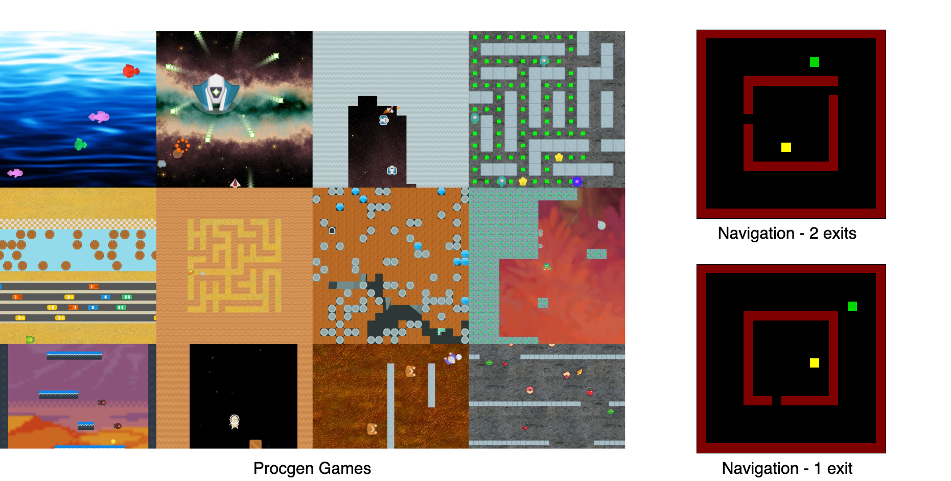
Figure 1: An illustrative example showcasing the Procgen games (on the left) juxtaposed with the Grid Navigation task (on the right).

E.1.1 Grid Navigation

The grid navigation task serves as a foundational test that mimics the challenges a robot might face when navigating in a 2D grid environment. This environment provides both a quantitative metric and a qualitative visualisation to understand an agent’s capacity to generalise its policy. Specifically, this task involves a $20\times 20$ grid with a central hall. At the beginning of each episode, the robot is positioned at a random point within this central hall. Simultaneously, a goal position is sampled randomly at a location outside the hall, challenging the robot to find its way out and reach this target. There are two variations of this task. The first provides the robot with a single exit from the central hall, while the second offers two exits. The single-exit hall scenario is similar to the two-exit scenario but requires a longer-horizon planning to successfully evade the walls to exit the hall and reach the goal.

E.1.2 Procgen

Procgen is a unique suite consisting of 16 game-like environments, each of which is procedurally generated. This means that they are designed to present slightly altered challenges every time they are played. Such design intricacy makes Procgen an ideal choice to test an agent’s generalisation capabilities. It stands in contrast to other commonly used testing suites, like the renowned Atari 2600 games (Mnih et al., 2013; 2016; Badia et al., 2020). The diverse array of environments within Procgen emphasises the pivotal role of robust policy learning. The environmental diversity in Procgen underlines the importance of robust policy learning for successful generalisation. The open-source code for the environments is publicly accessible at https://github.com/openai/procgen.

E.2 Training Setup

Differentiable Tree Search (DTS) is a drop-in replacement for conventional Convolutional Neural Network (CNN) architectures and can be trained using both online and offline reinforcement learning algorithms. In this paper, we employ the offline reinforcement learning (Offline-RL) framework to focus on the sample complexity and generalisation capabilities of DTS when compared with the baselines. Offline-RL, often referred to as batch-RL, is the scenario wherein an agent learns its policy solely from a fixed dataset of experiences, without further interactions with the environment.

However, the Offline-RL framework does present significant challenges, especially when it comes to the generalisation capabilities of methods, even for seemingly straightforward tasks like navigation. Consider, for instance, that the optimal policy is employed to collect experiences from an environment. It would predominantly select the optimal actions at every state. This means that only a fraction of the vast state-action space would be covered in the dataset. As a result, the model might not learn about many interactions, such as what happens when it collides with a wall, due to the limited training data on such environment interactions. When this world model is then applied in an online search scenario, the search process might unknowingly venture into out-of-distribution state space. These explorations, stemming from the model’s limited generalisation capabilities, can lead to overly optimistic value predictions, subsequently affecting the Q-values computation at the root node. In practical terms, the online search might mistakenly believe it can travel through a wall to reach its goal more quickly and would then run into it.

However, the DTS design offers a solution to this problem by jointly optimising both the world model and the online search. During the training phase, when the online search strays into the out-of-distribution states, it might overestimate the value of these states. This overestimation would then influence the final output after the search. When such a mismatch between the post-search output and the expert action is detected, the gradient descent algorithm adjusts these overestimated values, effectively lowering them to align the final Q-values more closely with the expert action. As a direct consequence of this, by the end of the training phase, the search process will have effectively learned to ignore these the out-of-distribution states.

E.3 Training Data Collection

E.3.1 Navigation

For our navigation task, which is relatively small in size, we are able to compute the optimal policy for any given state and configuration. We employ the value iteration algorithm for this purpose, as detailed by Sutton & Barto (2018). At the beginning of each episode, we formulate a random passage through the central hall. Subsequently, we also randomly determine the starting position of the robot within the hall and its goal position outside of it. Taking a cue from our approach with Procgen, we collect a total of $1000$ expert trajectories for training. Each of these trajectories incorporates a sequence comprising states, actions, rewards, and Q-values observed throughout the episode.

E.3.2 Procgen

When it comes to Procgen, even though there isn’t a public repository of pre-trained models, there exists an open-source code base for Phasic Policy Gradient (PPG) (Cobbe et al., 2021). With this in hand, we could effectively train a robust policy for every individual Procgen game starting from the ground up. We rely on the default set of hyperparameters for training a specific policy for each game. Once equipped with these trained policies, we treat them as expert agents. Using these expert policies, we then gather expert trajectories for $1000$ successful episodes. Just like in the case of Navigation, each of these trajectories represents a sequence comprising states, actions, rewards, and Q-values observed throughout the episode.

E.4 Implementation Details

In an effort to assess the distinctive elements of each agent’s design, we ensure uniformity in the number of parameters across all agents. This is achieved by integrating the submodules from DTS into the network architecture of every agent. However, while the number of parameters are consistent, the way in which these submodules are utilised to construct the computation graph varies among agents.

E.4.1 DTS

DTS utilises the submodules in alignment with the algorithm presented in Section A. For our empirical evaluations, we set the maximum limit for search trials at 10. Throughout the training process, the computation graph, formulated via online search, is optimised to accurately predict the Q-values. This optimisation serves a dual purpose: it not only refines the Q-value predictions but also facilitates robust learning for the submodules when they are employed in context of online search. The loss function designated for DTS training is:

$$\mathcal{L}_{DTS}=\lambda_{1}\mathcal{L}_{Q}+\lambda_{2}\mathcal{L}_{\mathcal{D}}+\lambda_{3}\mathcal{L}_{\mathcal{T}_{\theta}}+\lambda_{4}\mathcal{L}_{\mathcal{R}_{\theta}}$$

E.4.2 Model-free Q-Network

In this baseline, the submodules are utilise to perform a one-step look-ahead search. The input state undergoes an expansion using the world model, and Q-values are computed using the Bellman equation represented as $Q(s,a)=Rew(h,a)+Val(h^{\prime})$, where $h=Enc(s)$ and $h^{\prime}=Tr(h,a)$. Intriguingly, this structure does encapsulate a basic inductive bias via the 1-step look-ahead search. However, in keeping with its model-free characteristic, auxiliary losses aren’t employed for training the transition and reward model. The loss function for this model is:

$$\mathcal{L}_{Qnet}=\lambda_{1}\mathcal{L}_{Q}+\lambda_{2}\mathcal{L}_{\mathcal{D}}$$

E.4.3 TreeQN

In this baseline, the starting step is encoding the input state to its latent counterpart with the Encoder module. Following this, a full-tree expansion, based on a predefined depth $d$, is performed using both Transition and Reward modules. The values at the leaf nodes are then backpropagated to the root node via the Bellman equation, as discussed in the Backup phase in Section 3.2. The root node Q-values serve as the final output, that is utilised for training. Given the exponential growth of TreeQN’s computation graph with an increase in depth $d$, we choose a depth of 2 for our analysis, as recommended by TreeQN’s original code base (Farquhar et al., 2018). The associated loss function is:

$$\mathcal{L}_{TreeQN}=\lambda_{1}\mathcal{L}_{Q}+\lambda_{2}\mathcal{L}_{\mathcal{D}}+\lambda_{3}\mathcal{L}_{\mathcal{R}_{\theta}}$$

E.4.4 Online Search with Separately Learnt World Model

For this approach, we employ the best-first algorithm showcased in DTS. However, there’s a divergence: the world model and the value module are trained independently, each focusing on their specific objectives. As outlined in (Ye et al., 2021), we incorporate self-supervised consistency losses defined in Equation 7 and 8 as they improve the online search, even in cases where the world model is not jointly trained with the online search. The Q-values used for training are computed directly using the value module without performing online search during training. The loss function tailored for this approach is:

$$\mathcal{L}_{Search}=\lambda_{1}\mathcal{L}_{Q}+\lambda_{2}\mathcal{L}_{\mathcal{D}}+\lambda_{3}\mathcal{L}_{\mathcal{T}_{\theta}}+\lambda_{4}\mathcal{L}_{\mathcal{R}_{\theta}}$$

E.5 Issue with Baseline Normalised Score

Within the context of Atari games, the Baseline Normalised Score (BNS) is frequently utilised to evaluate the performance of agents. When human players are used as the baseline, it is often termed Human Normalised Score. The primary allure of BNS lies in its capacity to offer a relative assessment of an agent’s performance, comparing it against a standard benchmark—this could be human players or even another agent.

One of the primary benefits of the BNS is its ability to provide a consistent metric across different games, addressing the difference in scale inherent in raw scores. By enabling the calculation of the average BNS across multiple games, we gain insight into the overall efficacy of an agent. This not only facilitates direct performance comparisons between diverse agents and methodologies but also paints a picture of how the agent’s abilities stack up against human standards.

To derive the BNS, we start by logging the agent’s raw score in an Atari game. This raw score is then normalised against a baseline score, derived from baseline agent’s performance on the same game. By dividing the agent’s score by the baseline’s score (and sometimes subtracting the score of a random agent), we get a relative metric. Mathematically, this can be represented as:

$$BNS(\pi)=\dfrac{S_{\pi}-S_{R}}{S_{B}-S_{R}}$$ (21)

Here, $S_{\pi},S_{B}$ and $S_{R}$ denote the raw scores of the agent, the baseline policy, and a random policy, respectively. Interpretation-wise, a BNS of 1 indicates parity with the baseline. Values exceeding 1 signify outperformance, while those below 1 indicate underperformance relative to the baseline.

Nevertheless, the BNS has its frailties. It inherently presumes the baseline policy will always surpass the performance of the random policy. But there can be instances, contingent on the environment or the specific baseline policy, where this isn’t the case. In scenarios where the baseline policy underperforms the random policy, the BNS results in a negative denominator. This poses a predicament: even if our agent’s policy performs better than the random policy, the BNS unfairly penalises it. In our experiments with Procgen, we observed that for 2 out of the 16 games, namely heist and maze, the baseline policy underperformed compared to the random policy. Given these pitfalls, our evaluations pivot towards a more robust metric: the Z-score. The Z-score, often termed as the "standard score," provides a statistical measurement that describes a value’s relationship to the mean of a group of values. It is measured in terms of standard deviations from the mean. If a Z-score is 0, it indicates that the data point’s score is identical to the mean score. Z-scores may be positive or negative, with a positive value indicating the score is above the mean and a negative score indicating it is below the mean.

References

- Badia et al. (2020) Adrià Puigdomènech Badia, Bilal Piot, Steven Kapturowski, Pablo Sprechmann, Alex Vitvitskyi, Zhaohan Daniel Guo, and Charles Blundell. Agent57: Outperforming the atari human benchmark. In Proceedings of the 37th International Conference on Machine Learning, ICML 2020, 13-18 July 2020, Virtual Event, volume 119 of Proceedings of Machine Learning Research, pp. 507–517. PMLR, 2020. URL http://proceedings.mlr.press/v119/badia20a.html.
- Berner et al. (2019) Christopher Berner, Greg Brockman, Brooke Chan, Vicki Cheung, Przemyslaw Debiak, Christy Dennison, David Farhi, Quirin Fischer, Shariq Hashme, Christopher Hesse, Rafal Józefowicz, Scott Gray, Catherine Olsson, Jakub Pachocki, Michael Petrov, Henrique Pondé de Oliveira Pinto, Jonathan Raiman, Tim Salimans, Jeremy Schlatter, Jonas Schneider, Szymon Sidor, Ilya Sutskever, Jie Tang, Filip Wolski, and Susan Zhang. Dota 2 with large scale deep reinforcement learning. CoRR, abs/1912.06680, 2019. URL http://arxiv.org/abs/1912.06680.
- Chua et al. (2018) Kurtland Chua, Roberto Calandra, Rowan McAllister, and Sergey Levine. Deep reinforcement learning in a handful of trials using probabilistic dynamics models. In Samy Bengio, Hanna M. Wallach, Hugo Larochelle, Kristen Grauman, Nicolò Cesa-Bianchi, and Roman Garnett (eds.), Advances in Neural Information Processing Systems 31: Annual Conference on Neural Information Processing Systems 2018, NeurIPS 2018, December 3-8, 2018, Montréal, Canada, pp. 4759–4770, 2018. URL https://proceedings.neurips.cc/paper/2018/hash/3de568f8597b94bda53149c7d7f5958c-Abstract.html.
- Cobbe et al. (2020) Karl Cobbe, Christopher Hesse, Jacob Hilton, and John Schulman. Leveraging procedural generation to benchmark reinforcement learning. In Proceedings of the 37th International Conference on Machine Learning, ICML 2020, 13-18 July 2020, Virtual Event, volume 119 of Proceedings of Machine Learning Research, pp. 2048–2056. PMLR, 2020. URL http://proceedings.mlr.press/v119/cobbe20a.html.
- Cobbe et al. (2021) Karl Cobbe, Jacob Hilton, Oleg Klimov, and John Schulman. Phasic policy gradient. Proceedings of the 38th International Conference on Machine Learning, ICML 2021, 18-24 July 2021, Virtual Event, 139:2020–2027, 2021. URL http://proceedings.mlr.press/v139/cobbe21a.html.
- Deisenroth & Rasmussen (2011) Marc Peter Deisenroth and Carl Edward Rasmussen. PILCO: A model-based and data-efficient approach to policy search. In Lise Getoor and Tobias Scheffer (eds.), Proceedings of the 28th International Conference on Machine Learning, ICML 2011, Bellevue, Washington, USA, June 28 - July 2, 2011, pp. 465–472. Omnipress, 2011. URL https://icml.cc/2011/papers/323_icmlpaper.pdf.
- Espeholt et al. (2018) Lasse Espeholt, Hubert Soyer, Remi Munos, Karen Simonyan, Vlad Mnih, Tom Ward, Yotam Doron, Vlad Firoiu, Tim Harley, Iain Dunning, et al. Impala: Scalable distributed deep-rl with importance weighted actor-learner architectures. In International Conference on Machine Learning, pp. 1407–1416. PMLR, 2018.
- Farquhar et al. (2018) Gregory Farquhar, Tim Rocktäschel, Maximilian Igl, and Shimon Whiteson. Treeqn and atreec: Differentiable tree-structured models for deep reinforcement learning. In 6th International Conference on Learning Representations, ICLR 2018, Vancouver, BC, Canada, April 30 - May 3, 2018, Conference Track Proceedings. OpenReview.net, 2018. URL https://openreview.net/forum?id=H1dh6Ax0Z.
- Guez et al. (2018) Arthur Guez, Théophane Weber, Ioannis Antonoglou, Karen Simonyan, Oriol Vinyals, Daan Wierstra, Rémi Munos, and David Silver. Learning to search with mctsnets. In International Conference on Machine Learning, pp. 1822–1831. PMLR, 2018.
- Guez et al. (2019) Arthur Guez, Mehdi Mirza, Karol Gregor, Rishabh Kabra, Sébastien Racanière, Théophane Weber, David Raposo, Adam Santoro, Laurent Orseau, Tom Eccles, et al. An investigation of model-free planning. In International Conference on Machine Learning, pp. 2464–2473. PMLR, 2019.
- Ha & Schmidhuber (2018) David Ha and Jürgen Schmidhuber. Recurrent world models facilitate policy evolution. In Advances in Neural Information Processing Systems 31: Annual Conference on Neural Information Processing Systems 2018, NeurIPS 2018, December 3-8, 2018, Montréal, Canada, pp. 2455–2467, 2018. URL https://proceedings.neurips.cc/paper/2018/hash/2de5d16682c3c35007e4e92982f1a2ba-Abstract.html.
- Hafner et al. (2019) Danijar Hafner, Timothy P. Lillicrap, Ian Fischer, Ruben Villegas, David Ha, Honglak Lee, and James Davidson. Learning latent dynamics for planning from pixels. In Proceedings of the 36th International Conference on Machine Learning, ICML 2019, 9-15 June 2019, Long Beach, California, USA, volume 97 of Proceedings of Machine Learning Research, pp. 2555–2565. PMLR, 2019. URL http://proceedings.mlr.press/v97/hafner19a.html.
- Hafner et al. (2020) Danijar Hafner, Timothy P. Lillicrap, Jimmy Ba, and Mohammad Norouzi. Dream to control: Learning behaviors by latent imagination. In 8th International Conference on Learning Representations, ICLR 2020, Addis Ababa, Ethiopia, April 26-30, 2020. OpenReview.net, 2020. URL https://openreview.net/forum?id=S1lOTC4tDS.
- Hessel et al. (2018) Matteo Hessel, Joseph Modayil, Hado Van Hasselt, Tom Schaul, Georg Ostrovski, Will Dabney, Dan Horgan, Bilal Piot, Mohammad Azar, and David Silver. Rainbow: Combining improvements in deep reinforcement learning. In Thirty-second AAAI conference on artificial intelligence, 2018.
- Hessel et al. (2019) Matteo Hessel, Hado van Hasselt, Joseph Modayil, and David Silver. On inductive biases in deep reinforcement learning. CoRR, abs/1907.02908, 2019. URL http://arxiv.org/abs/1907.02908.
- Kaiser et al. (2020) Lukasz Kaiser, Mohammad Babaeizadeh, Piotr Milos, Blazej Osinski, Roy H. Campbell, Konrad Czechowski, Dumitru Erhan, Chelsea Finn, Piotr Kozakowski, Sergey Levine, Afroz Mohiuddin, Ryan Sepassi, George Tucker, and Henryk Michalewski. Model based reinforcement learning for atari. In 8th International Conference on Learning Representations, ICLR 2020, Addis Ababa, Ethiopia, April 26-30, 2020. OpenReview.net, 2020. URL https://openreview.net/forum?id=S1xCPJHtDB.
- Kumar et al. (2020) Aviral Kumar, Aurick Zhou, George Tucker, and Sergey Levine. Conservative q-learning for offline reinforcement learning. Advances in Neural Information Processing Systems 33: Annual Conference on Neural Information Processing Systems 2020, NeurIPS 2020, December 6-12, 2020, virtual, 2020. URL https://proceedings.neurips.cc/paper/2020/hash/0d2b2061826a5df3221116a5085a6052-Abstract.html.
- Lee et al. (2018) Lisa Lee, Emilio Parisotto, Devendra Singh Chaplot, Eric Xing, and Ruslan Salakhutdinov. Gated path planning networks. In International Conference on Machine Learning, pp. 2947–2955. PMLR, 2018.
- Mittal et al. (2023) Dixant Mittal, Siddharth Aravindan, and Wee Sun Lee. Expose: Combining state-based exploration with gradient-based online search. In Proceedings of the 2023 International Conference on Autonomous Agents and Multiagent Systems, AAMAS ’23, pp. 1345–1353, Richland, SC, 2023. International Foundation for Autonomous Agents and Multiagent Systems. ISBN 9781450394321.
- Mnih et al. (2013) Volodymyr Mnih, Koray Kavukcuoglu, David Silver, Alex Graves, Ioannis Antonoglou, Daan Wierstra, and Martin A. Riedmiller. Playing atari with deep reinforcement learning. CoRR, abs/1312.5602, 2013. URL http://arxiv.org/abs/1312.5602.
- Mnih et al. (2016) Volodymyr Mnih, Adrià Puigdomènech Badia, Mehdi Mirza, Alex Graves, Timothy P. Lillicrap, Tim Harley, David Silver, and Koray Kavukcuoglu. Asynchronous methods for deep reinforcement learning. In Maria-Florina Balcan and Kilian Q. Weinberger (eds.), Proceedings of the 33nd International Conference on Machine Learning, ICML 2016, New York City, NY, USA, June 19-24, 2016, volume 48 of JMLR Workshop and Conference Proceedings, pp. 1928–1937. JMLR.org, 2016. URL http://proceedings.mlr.press/v48/mniha16.html.
- Nagabandi et al. (2018) Anusha Nagabandi, Gregory Kahn, Ronald S. Fearing, and Sergey Levine. Neural network dynamics for model-based deep reinforcement learning with model-free fine-tuning. In 2018 IEEE International Conference on Robotics and Automation, ICRA 2018, Brisbane, Australia, May 21-25, 2018, pp. 7559–7566. IEEE, 2018. doi: 10.1109/ICRA.2018.8463189. URL https://doi.org/10.1109/ICRA.2018.8463189.
- Oh et al. (2017) Junhyuk Oh, Satinder Singh, and Honglak Lee. Value prediction network. Advances in neural information processing systems, 30, 2017.
- Pascanu et al. (2017) Razvan Pascanu, Yujia Li, Oriol Vinyals, Nicolas Heess, Lars Buesing, Sébastien Racanière, David P. Reichert, Theophane Weber, Daan Wierstra, and Peter W. Battaglia. Learning model-based planning from scratch. CoRR, abs/1707.06170, 2017. URL http://arxiv.org/abs/1707.06170.
- Racanière et al. (2017) Sébastien Racanière, Théophane Weber, David P Reichert, Lars Buesing, Arthur Guez, Danilo Rezende, Adria Puigdomenech Badia, Oriol Vinyals, Nicolas Heess, Yujia Li, et al. Imagination-augmented agents for deep reinforcement learning. In Proceedings of the 31st International Conference on Neural Information Processing Systems, pp. 5694–5705, 2017.
- Rudin (1976) Walter Rudin. Principles of Mathematical Analysis. McGraw-Hill New York, 3d ed. edition, 1976. ISBN 007054235. URL http://www.loc.gov/catdir/toc/mh031/75017903.html.
- Schrittwieser et al. (2020) Julian Schrittwieser, Ioannis Antonoglou, Thomas Hubert, Karen Simonyan, Laurent Sifre, Simon Schmitt, Arthur Guez, Edward Lockhart, Demis Hassabis, Thore Graepel, et al. Mastering atari, go, chess and shogi by planning with a learned model. Nature, 588(7839):604–609, 2020.
- Schulman et al. (2015a) John Schulman, Nicolas Heess, Theophane Weber, and Pieter Abbeel. Gradient estimation using stochastic computation graphs. In Corinna Cortes, Neil D. Lawrence, Daniel D. Lee, Masashi Sugiyama, and Roman Garnett (eds.), Advances in Neural Information Processing Systems 28: Annual Conference on Neural Information Processing Systems 2015, December 7-12, 2015, Montreal, Quebec, Canada, pp. 3528–3536, 2015a. URL https://proceedings.neurips.cc/paper/2015/hash/de03beffeed9da5f3639a621bcab5dd4-Abstract.html.
- Schulman et al. (2015b) John Schulman, Sergey Levine, Pieter Abbeel, Michael I. Jordan, and Philipp Moritz. Trust region policy optimization. In Proceedings of the 32nd International Conference on Machine Learning, ICML 2015, Lille, France, 6-11 July 2015, volume 37 of JMLR Workshop and Conference Proceedings, pp. 1889–1897. JMLR.org, 2015b. URL http://proceedings.mlr.press/v37/schulman15.html.
- Schulman et al. (2017) John Schulman, Filip Wolski, Prafulla Dhariwal, Alec Radford, and Oleg Klimov. Proximal policy optimization algorithms. arXiv preprint arXiv:1707.06347, 2017.
- Schwarzer et al. (2021) Max Schwarzer, Ankesh Anand, Rishab Goel, R. Devon Hjelm, Aaron C. Courville, and Philip Bachman. Data-efficient reinforcement learning with self-predictive representations. In 9th International Conference on Learning Representations, ICLR 2021, Virtual Event, Austria, May 3-7, 2021. OpenReview.net, 2021. URL https://openreview.net/forum?id=uCQfPZwRaUu.
- Shah et al. (2020) Ameesh Shah, Eric Zhan, Jennifer J. Sun, Abhinav Verma, Yisong Yue, and Swarat Chaudhuri. Learning differentiable programs with admissible neural heuristics. In Hugo Larochelle, Marc’Aurelio Ranzato, Raia Hadsell, Maria-Florina Balcan, and Hsuan-Tien Lin (eds.), Advances in Neural Information Processing Systems 33: Annual Conference on Neural Information Processing Systems 2020, NeurIPS 2020, December 6-12, 2020, virtual, 2020. URL https://proceedings.neurips.cc/paper/2020/hash/342285bb2a8cadef22f667eeb6a63732-Abstract.html.
- Silver et al. (2017a) David Silver, Hado Hasselt, Matteo Hessel, Tom Schaul, Arthur Guez, Tim Harley, Gabriel Dulac-Arnold, David Reichert, Neil Rabinowitz, Andre Barreto, et al. The predictron: End-to-end learning and planning. In International Conference on Machine Learning, pp. 3191–3199. PMLR, 2017a.
- Silver et al. (2017b) David Silver, Julian Schrittwieser, Karen Simonyan, Ioannis Antonoglou, Aja Huang, Arthur Guez, Thomas Hubert, Lucas Baker, Matthew Lai, Adrian Bolton, et al. Mastering the game of go without human knowledge. nature, 550(7676):354–359, 2017b.
- Sutton & Barto (2018) Richard S Sutton and Andrew G Barto. Reinforcement learning: An introduction. MIT press, 2018.
- Tamar et al. (2016) Aviv Tamar, Yi Wu, Garrett Thomas, Sergey Levine, and Pieter Abbeel. Value iteration networks. In Proceedings of the 30th International Conference on Neural Information Processing Systems, pp. 2154–2162, 2016.
- van Hasselt et al. (2016) Hado van Hasselt, Arthur Guez, and David Silver. Deep reinforcement learning with double q-learning. In Dale Schuurmans and Michael P. Wellman (eds.), Proceedings of the Thirtieth AAAI Conference on Artificial Intelligence, February 12-17, 2016, Phoenix, Arizona, USA, pp. 2094–2100. AAAI Press, 2016. doi: 10.1609/aaai.v30i1.10295. URL https://doi.org/10.1609/aaai.v30i1.10295.
- Vinyals et al. (2019) Oriol Vinyals, Igor Babuschkin, Wojciech M Czarnecki, Michaël Mathieu, Andrew Dudzik, Junyoung Chung, David H Choi, Richard Powell, Timo Ewalds, Petko Georgiev, et al. Grandmaster level in starcraft ii using multi-agent reinforcement learning. Nature, 575(7782):350–354, 2019.
- Wang et al. (2016) Ziyu Wang, Tom Schaul, Matteo Hessel, Hado van Hasselt, Marc Lanctot, and Nando de Freitas. Dueling network architectures for deep reinforcement learning. In Maria-Florina Balcan and Kilian Q. Weinberger (eds.), Proceedings of the 33nd International Conference on Machine Learning, ICML 2016, New York City, NY, USA, June 19-24, 2016, volume 48 of JMLR Workshop and Conference Proceedings, pp. 1995–2003. JMLR.org, 2016. URL http://proceedings.mlr.press/v48/wangf16.html.
- Williams (1992) Ronald J Williams. Simple statistical gradient-following algorithms for connectionist reinforcement learning. Machine learning, 8(3):229–256, 1992.
- Ye et al. (2021) Weirui Ye, Shaohuai Liu, Thanard Kurutach, Pieter Abbeel, and Yang Gao. Mastering atari games with limited data. In Marc’Aurelio Ranzato, Alina Beygelzimer, Yann N. Dauphin, Percy Liang, and Jennifer Wortman Vaughan (eds.), Advances in Neural Information Processing Systems 34: Annual Conference on Neural Information Processing Systems 2021, NeurIPS 2021, December 6-14, 2021, virtual, pp. 25476–25488, 2021. URL https://proceedings.neurips.cc/paper/2021/hash/d5eca8dc3820cad9fe56a3bafda65ca1-Abstract.html.
- Yonetani et al. (2021) Ryo Yonetani, Tatsunori Taniai, Mohammadamin Barekatain, Mai Nishimura, and Asako Kanezaki. Path planning using neural a* search. In Marina Meila and Tong Zhang (eds.), Proceedings of the 38th International Conference on Machine Learning, ICML 2021, 18-24 July 2021, Virtual Event, volume 139 of Proceedings of Machine Learning Research, pp. 12029–12039. PMLR, 2021. URL http://proceedings.mlr.press/v139/yonetani21a.html.