Mean uniformly stable function and its application to almost sure stability analysis of randomly switched time-varying systems

Abstract

This paper investigates almost sure stability of randomly switched time-varying systems. To assess stability properties of diverse time-varying subsystems, mode-dependent indefinite multiple Lyapunov functions are introduced. We present a novel condition so-called mean uniformly stable function focusing on the time-varying functions in derivatives’ parameters of indefinite multiple Lyapunov functions. This condition doesn’t need pre-determined switching moments and provides enhanced flexibility to accommodate unstable subsystems and stable but no-exponentially decay subystems. A numerical example is provided to demonstrate the effectiveness and advantages of our approach.

I Introduction

As an important class of dynamics, switched systems have received extensively investigations over the last few decades. Among these systems, randomly switched systems have garnered increasing attention due to their significance in both theoretical developments of practical systems with random structural changes, such as flight systems, power systems, communication systems, and networked control systems. A randomly switched systems consists of a collection of subsystems and a random switching signal that dictates the transitions between subsystems, where semi-Markov chains (including Markov chains) and renewal processes are commonly employed as switching signals (see the detail in [1, 2, 3, 4, 5]).

Stability plays an important and fundamental role in the dynamic analysis and control design of systems. Most concerned stability concepts of randomly switched systems are stability in probability, $p$th moment stability and almost sure stability [1, 4, 5]. Almost sure stability provides crucial convergence insights regarding behavior of individual trajectories of states in an ”almost all” sense. This concept has demonstrated practical usefulness and effectiveness in various studies [3, 4, 6], and it serves as the primary focus of investigation in this work.

In recent years, stability analysis of time-varying systems has been the subject of numerous studies. Recognizing that the classical Lyapunov functions with strict negative derivatives are not sufficient for the stability analysis of time-varying systems (see Example 1 in [7]), researchers have explored the idea of replacing the negative defined constant parameter of the time derivative of Lyapunov function with a time-varying function, i.e.,

$$\dot{V}(t,x(t))\leq\lambda(t)V(t,x(t)).$$ (1)

Coincidentally, earliest in 1959, Krasovskii has pointed out that the stability estimation of a time-varying system may assume that the derivatives of Lyapunov functions have time-varying parameters (Theorem 10.3 in [8]). This form was applied into time-varying systems with impulsive and Markov switching in [9], and was promptly extended to impulsive time-varying systems [10, 11] and stochastic hybrid systems [12]. It is noteworthy that form (1) endows derivatives of Lyapunov functions to be indefinitely signed, i.e., $\lambda(t)\in\mathbb{R}$, and thus has been named as indefinite Lyapunov functions method (iLFs) [13, 14, 15, 16].

The crucial part of establish stability criteria through iLFs (1) is the treatment of time-varying function $\lambda(t)$, where the ultimate goal is to achieve the decay of Lyapunov function facilitated by $\lambda(t)$. In [8], Krasovskii firstly obtained global asymptotic stability (GAS) criterion by assuming that the integral of $\lambda(t)$ in (1) tends to $-\infty$ as $t$ tends to $\infty$. In [9] and [12], scholars adopted conditions that integral of positive part of $\lambda(t)$ is finite for any $t$ and integral of negative part of $\lambda(t)$ is tending to $-\infty$ when $t$ tends to $\infty$. Considering that the uniformity of stability and attractivity is an important challenge for time-varying systems, Ning et al. presented a positive linear function of time interval as constraint on integral of $\max\{-\lambda(t),0\}$ to obtain global uniform asymptotic stability (GUAS) and uniform global exponential stability (GUES) criteria [13, 14, 15, 16]. In [17, 18, 7], Zhou et al. further refined these conditions for time-varying functions, establishing relationships between these conditions and stability concepts through a linear time-varying differential equality. These conditions for time-varying functions are therefore named as ”stable functions”. In specific, GAS criterion can be obtained through iLFs (1) with asymptotic stable functions (ASF):

$$\int_{t_{0}}^{\infty}\lambda(h)\mathrm{d}h=-\infty,$$ (2)

and criteria of GUAS and GUES can be gotten by iLFs (1) with exponential stable functions (UESF):

$$\int_{t_{0}}^{t}\lambda(h)\mathrm{d}h\leq-a(t-t_{0})+b.$$ (3)

More details are available in [17, 18, 7].

Back to randomly switched systems, since they share same mathematical description with deterministic switched systems except switching signals, one can adopt multiple Lyapunov functions (MLFs) method to conduct stability analysis. This method, presented by [19], is designed to estimate each subsystem’s stability property individually in analysis of deterministic switched [20]. It assumes that for $i$th subsystem, with switching mode $r(t)=i$, there holds stability estimation:

$$\dot{V}_{i}(x(t))\leq c_{i}V_{i}(x(t)),$$ (4)

An outstanding advantage of MLFs method applying into randomly switched systems is that derivatives of MLFs have mode-dependent constant coefficients. By setting $c_{i}$ in (4) be real numbers, this method can consider the cases where subsystems may perform different decay rates of stability and even some of them are unstable [21, 22, 23].

For switched time-varying systems, it is natural to combine MLFs (4) with iLFs (1) for time-varying subsystems. Then a so-called indefinite multiple Lyapunov function (iMLF) (5) is presented

$$\dot{V}_{i}(t,x(t))\leq\lambda(t)V_{i}(t,x(t)).$$ (5)

This stability estimator is effectively employed to investigate deterministic switched time-varying systems [24, 25, 26, 27], time-varying systems with Markov switching [28] and semi-Markov switching [29].

However, for a switched time-varying system, the stability estimator for every subsystem may be specific. Hence, mode-dependent iMLFs method is presented [30, 31], specifying, for $i$th subsystem, there holds:

$$\dot{V}_{i}(t,x(t))\leq\lambda_{i}(t)V_{i}(t,x(t)).$$ (6)

In addition, global constraints on $\lambda_{\sigma(t)}(t)$ are introduced in relation to switching signals $\sigma(t)$ with the average dwell time condition. Suppose that the switching dwell time interval is $[t_{k},t_{k+1})$. Then, in [30], the following condition (7) similar to ASF (2) is given: for any $t\in[t_{k},t_{k+1}),\ k=0,1,\cdots$,

$$\int_{t_{0}}^{\infty}\lambda_{\sigma(h)}(h)\mathrm{d}h=\lim_{k\rightarrow\infty}\sum_{l=0}^{k}\int_{t_{l}}^{t_{l+1}}\lambda_{\sigma(t_{l})}(h)\mathrm{d}h=-\infty,$$ (7)

and in order to ensure uniformity of attractivity and stability, the following restriction (8) is given in [30]

$$\int_{t_{k}}^{t}\lambda_{\sigma(t_{k})}(h)\mathrm{d}h<M.$$ (8)

On the other hand, Wu et al. presented the following condition (I) similar to UESF (2) in [31]

$$\int_{t_{0}}^{t}\lambda_{\sigma(h)}(h)\mathrm{d}h= \sum_{l=0}^{k-1}\int_{t_{l}}^{t_{l+1}}\lambda_{\sigma(t_{l})}(h)\mathrm{d}h+\int_{t_{k}}^{t}\lambda_{\sigma(t_{k})}(h)\mathrm{d}h$$

$$\leq -a(t-t_{0})+b.$$ (9)

As can be seen in (7)-(I), switching moments $t_{k}$ should be pre-determined according to switching signal. Unfortunately, randomly switching signals $r(t)$ may have random switching moments and random dwell time. Therefore, $t_{k}$ may be unknown such that the conditions (7)-(I) cannot be verified in practical application.

In order to overcome the limition of the conditions (7)-(I) mentioned above, the so-called mean uniformly stable function (MUSF) on $\lambda_{r(t)}(t)$ is presented in this paper, where $r(t)$ denotes a randomly switching signal. The specific restrictions are given on every $\lambda_{i}(t)$ that their integrals about random dwell time intervals are mean bounded, which no need to know switching moments $t_{k}$. Additionally, MUSF is uniform over time, and thus can ensure the uniformity of stability and attractivity. Based on the MUSF, we can thereby establish almost sure stability criteria for randomly switched time-varying systems, assuming switching signals satisfy semi-Markov process, Markov process and renewal process. Advantages and effectiveness of our results will be demonstrated through numerical examples.

Notations: Let $(\Omega,\mathcal{F},\mathcal{F}_{t},\mathbb{P})$ be a complete probability space. $\mathbb{R}^{n\times m}$ denotes the $n\times m$-dimensional Euclidean space, $\mathbb{R}^{+}=[0,+\infty)$, $\mathbb{R}_{t_{0}}^{+}=[t_{0},+\infty)$. $\left|\cdot\right|$ denotes the Euclidean norm. $\mathbb{N}^{+}$ denotes nonnegative integers. $\mathcal{K}$ denotes the class of strictly increasing continuous functions, $\mathcal{K}_{\infty}$ is the subset of $\mathcal{K}$ where functions trend to infinity as $t\rightarrow\infty$. Let $\mathcal{KL}$ be the class of functions with strictly increasing first variable and decreasing second variable. $\mathcal{C}^{1,2}(\mathbb{R}^{+}_{t_{0}},\mathbb{R}^{n};\mathbb{R}^{n})$ represents the family of all $\mathbb{R}^{n}$-valued functions whose first variable’s derivative is continuous and second variable’s second derivative is continuous. Moreover, $\mathcal{PC}(\mathbb{R}^{+}_{t_{0}};\mathbb{R})$ represents the family of all piece-wise continuous function.

II Model formulation and preliminaries

Considering the following time-varying randomly switched systems:

$$\begin{cases}\dot{x}(t)=f_{r}(t,x(t)),\\ x(t_{0})=\phi,\end{cases}$$ (10)

where $x(t)\in\mathbb{R}^{n}$ is state, $r(t)\in\mathbb{S}\subset\mathbb{N}^{+}$ is the switching signal and also a cádlág stochastic process, where $\mathbb{S}$ is set of the switch modes. For all $r(t)=i\in\mathbb{S}$, $f_{i}$ satisfy the locally Lipschitz condition and $f_{i}(t,0,0)=0$. The set of switching moments is defined by $\mathcal{T}=\{t_{0}\leq t_{1}\leq t_{2}\leq\cdots\leq t_{k}\leq\cdots,\ k\in\mathbb{N}^{+}\}$. $N_{i}(t,s)$ represents the occurrence counts of $i$th subsystem during $[s,t]$, and we note $r(t_{0})=r_{0}$. The counting function

$$N(t,s)=\sum_{i\in\mathbb{S}}N_{i}(t,s)$$ (11)

is the switch counts of switching signal in the interval $[s,t]$. $S(k)=t_{k}-t_{k-1},\ k\in\mathbb{N}^{+}$ is $k$-th dwell time between switches. And when $t\in[t_{k-1},t_{k}]$ we assume $r(t)=i$, then denote $S_{i}(k)$ as the running time of $i$-th system during the $k$-th dwell time. $T_{i}(t,s)=\sum_{k=1}^{N_{i}(t,s)}S_{i}(k)$ is the total running time of $i$th system among time interval $[s,t]$. We present following definition of randomly switched signals.

In this work, we mainly consider the following randomly switching signals.

Definition 1 ([32]).

The switching signal $r(t)$ is said to be

1. semi-Markov switching signal, if for $t\in[t_{k-1},t_{k}]$ embedded process $r(t)=r_{k}$ is a discrete-time Markov chain with transition probability matrix $P=[p_{ij}]$, where $p_{ij}:=\mathbb{P}[r_{k+1}=j|r_{k}=i]$. The dwell time $S(k)=t_{k}-t_{k-1}$ is random variable with distribution function

   $$F_{ij}(t)\!=\!\mathbb{P}\left[S(k)\!\leq\!t|r_{k}\!=\!j,r_{k\!-\!1}\!=\!i\right],i,j\in\mathbb{S},t\!\geq\!t_{0}.$$

   $r_{k}$ and $S(k)$ are independent and memory-less i.e.

   $$\mathbb{P}\left[r_{k}=i,S(k)\leq t|\cup_{l=1}^{k-1}\left\{r_{l},S(l)\right\}\right]$$

   $$= \mathbb{P}\left[r_{k}\!=\!i,S(k)\!\leq\!t|r_{k-1}\right],i\in\mathbb{S},t\geq t_{0}.$$

2. Markov switching signal, if for $t\in[t_{k-1},t_{k}],\ k\in\mathbb{N}^{+}$, $r(t)=r_{k}$ there holds

   $$\mathbb{P}\left[r_{k}=i|\cup_{l=1}^{k-1}\left\{r_{l}\right\}\right]=\mathbb{P}\left[r_{k}=i|r_{k-1}\right],i\in\mathbb{S},t\geq t_{0}.$$

   And its generator $Q=[q_{ij}]$ is defined by

   $$\mathbb{P}\left[r(t+h)=j|r(t)=i\right]=\begin{cases}q_{ij}h+o(h),\ &i\neq j\\ 1+q_{ij}h+o(h),\ &i=j\end{cases}$$

   where $h>0$, $\lim_{h\rightarrow 0}\frac{o(h)}{h}=0$ and $q_{ii}=-\sum_{j\neq i}q_{ij}$.

3. renewal process switching, if the switching counts $N(t,t_{0})$ satisfies a renewal process, that is, the dwell times $\{S(k),k\in\mathbb{N}^{+}\}$ are a sequence of nonnegative independent random variables with a common distribution $F$.

Lemma 1 ([21, 22, 31]).

The randomly switching signal $r(t)$ has the following properties.

1. If $r(t)$ is an irreducible semi-Markov chain, that is its embedded Markov chain is irreducible, then it has stationary distribution

   $$\lim_{t\rightarrow\infty}\mathbb{P}[r(t)=i]=\lim_{t\rightarrow\infty}\frac{T_{i}(t,t_{0})}{t-t_{0}}=\pi_{i},\ \mathrm{a.s.}$$

   where

   $$\pi_{i}=\frac{\bar{\pi}_{i}m_{i}}{\sum_{j\in\mathbb{S}}\bar{\pi}_{j}m_{j}},\ i\in\mathbb{S},$$

   and $\bar{\pi}=[\bar{\pi}_{i}]_{1\times M}$ represents the stationary distribution of discrete embedded Markov chain. And by ergodic theory, there holds

   $$\lim_{t\rightarrow\infty}\frac{N_{i}(t,t_{0})}{t-t_{0}}=\frac{\pi_{i}}{m_{i}},\ \mathrm{a.s.}$$

   where $\mathbb{E}[{S_{i}(k)}]=m_{i},\ k\in\mathbb{N}^{+}$.

2. If $r(t)$ is an irreducible Markov chain has stationary

   $$\lim_{t\rightarrow\infty}\mathbb{P}[r(t)=i]=\pi_{i},\ \mathrm{a.s.}$$

   and by its ergodicity, there holds

   $$\lim_{t\rightarrow\infty}\frac{N_{i}(t,t_{0})}{t-t_{0}}=\pi_{i}q_{i},\ \mathrm{a.s.}$$

   where $q_{i}=|q_{ii}|,\ i\in\mathbb{S}$.

3. If $r(t)$ is a renewal process, which means $N(t,t_{0})$ is a renewal process, then

   $$\lim_{t\rightarrow\infty}\frac{N(t,t_{0})}{t-t_{0}}=\frac{1}{\theta},\ \mathrm{a.s.}$$

   where $\mathbb{E}[S(k)]=\theta$. And there exists a probability distribution

   $$\mathbb{P}[r(t_{k+1})=i|r(t_{k}),\cdots,r(t_{0})]=p_{i}.$$

Definition 2.

System (10) is said to be:

1. almost surely uniformly stable (US a.s.), if for each $\epsilon>0$, there exists a constant $\delta=\delta(\epsilon)>0$, such that when $|\phi|<\delta$,

   $$\mathbb{P}\left[\sup_{t\geq t_{0}}|x(t)|<\epsilon\right]=1;$$

2. almost surely uniformly attractive (UA a.s.), if for any $t_{0},\epsilon^{\prime}>0$, there exist $\rho>0$ and $T=T(\epsilon^{\prime})\geq 0$ so that when $|\phi|<\rho$,

   $$\mathbb{P}\left[\sup_{t\geq T+t_{0}}|x(t)|<\epsilon^{\prime}\right]=1;$$

3. almost surely globally uniformly asymptotically stable (GUAS a.s.), if (1) and (2) are both fulfilled for all $\phi\in\mathbb{R}^{n}$;

4. almost surely globally exponential stable (GES a.s.), if

   $$\limsup_{t\rightarrow\infty}\frac{1}{t}\ln|x(t)|<0,\ \mathrm{a.s.}$$ (12)

   holds for all $\phi\in\mathbb{R}^{n}$.

III Main Results

In this section, we will present novel mean uniformly functions for iMLFs to establish sufficient conditions for almost sure GUAS and GES. As we delve into this section, it will show that mean uniformly functions hold their significance in stability analysis of randomly switching time-varying systems.

III-A Indefinite multiple Lyapunov functions and mean uniformly functions

Mode-dependent iMLFs scheme is given as following.

Assumption 1.

For all $i\in\mathbb{S}$, $V_{i}\in\mathcal{C}^{1,2}(\mathbb{R}_{t_{0}}^{+},\mathbb{R}^{n};\mathbb{R}^{+})$ are said to be iMLFs, if there exists $\lambda_{i}\in\mathcal{PC}(\mathbb{R}_{t_{0}}^{+};\mathbb{R})$, $\alpha_{1},\alpha_{2}\in\mathcal{K}_{\infty}$, $\rho\in\mathcal{K}_{\infty}$, and a positive constant $\mu>1$ such that

1. $\alpha_{1}(|x(t)|)\leq V_{i}(t,x(t))\leq\alpha_{2}(|x(t)|),\ \forall i\in\mathbb{S};$

2. for all $t\in\mathbb{R}_{t_{0}}^{+}\backslash\mathcal{T}$ and $i\in\mathbb{S}$,

   $$\dot{V}_{i}(t,x(t))\leq\lambda_{i}(t)V_{i}(t,x(t));$$ (13)

3. for all $t\in\mathcal{T}$,

   $$V_{i}(t,x(t))\leq\mu_{i}V_{j}(t,x(t)).$$ (14)

Stability estimators for every time-varying subsystems are given through iMLFs scheme. Then following conditions on $\lambda_{i}(t)$ is required, named as mean uniformly function, to further establish the stability criteria.

Definition 3.

The scalar function $\lambda(t)\in\mathcal{PC}(\mathbb{R}^{+};\mathbb{R})$ is said to be

• a mean uniformly stable function (MUSF), if for any random variable $S>0$ with $\mathbb{E}[S]<\infty$ there exists a constant $\hat{M}\in\mathbb{R}$ such that

  $$\mathbb{E}\left[\int_{t}^{t+S}\lambda(h)\mathrm{d}h\right]\leq\hat{M},\ \forall t\geq t_{0}.$$ (15)

• a mean uniformly stable function with respect to $\varphi$ (MUSF w.r.t. $\varphi$), if for any random variable $S>0$ with $\mathbb{E}[S]<\infty$, there exists a function $\varphi(t)\in\mathcal{PC}(\mathbb{R}^{+};\mathbb{R})$ such that

  $$\mathbb{E}\left[\int_{t}^{t+S}\lambda(h)\mathrm{d}h\right]\leq\mathbb{E}\left[\varphi\left(S\right)\right],\ \forall t\geq t_{0}.$$ (16)

• a mean uniformly exponential stable function (MUESF), if for any random variable $S>0$ with $\mathbb{E}[S]<\infty$, there exists a constant $\bar{\lambda}\in\mathbb{R}$ such that

  $$\mathbb{E}\left[\int_{t}^{t+S}\lambda(h)\mathrm{d}h\right]\leq\mathbb{E}\left[\bar{\lambda}S\right],\ \forall t\geq t_{0}.$$ (17)

Remark.

It is obviously that a MUESF must be a MUSF w.r.t. $\varphi$ where $\varphi(t)=\bar{\lambda}t$. Additionally, MUSF w.r.t. $\varphi$ must be a MUSF, because of measurable property of $\varphi(t)$ resulted by its piece-wise continuity. The relationship between these mean uniformly functions are shown as following:

$$\mathrm{MUESF}\subset\mathrm{MUSF\ w.r.t.}\ \varphi\subset\mathrm{MUSF}.$$

Remark.

There three primary reasons behind the nomenclature ’mean uniformly functions’ for the conditions in Definition 3. Firstly, each $\lambda_{i}(t)$ operates exclusively during the relative subsystem’s dwell time, which is random variable. To capture variations of $\lambda_{i}(t)$, we employ the expectation to quantify it integral. Secondly, $\lambda_{i}(t)$ has potential to take positive value during the dwell time, and piece-wise continuity yields that integral of $\lambda_{i}(t)$ would be bounded in mean, constituting a form of mean stability. It is evident that mean uniformly functions facilitate the existence of certain unstable time-varying subsystems, as exemplified in the aforementioned discussion. Third, as shown in (15), (16) and (17), these conditions solely depend on the random variable $S$ and thus are uniform in time, which can ensure stability uniformity.

To further obtain almost sure GUAS through mean uniformly functions, we shall conduct a specific analysis based on the particular randomly switching signal.

III-B Almost sure stability of time-varying systems with semi-Markov switching

Theorem 1.

If Assumption 1 and following condition hold:

if $\lambda_{i}(t)$ are MUSFs w.r.t. $\varphi_{i}$ for all $i\in\mathbb{S}$ and $\sum_{i\in\mathbb{S}}(\mathbb{E}\left[\varphi_{i}(S_{i})\right]+\ln\mu_{i})\frac{\pi_{i}}{m_{i}}<0$.

Then semi-Markov switched system (10) is GUAS a.s.

Proof.

Without loss of generality, we assume that $t_{0}=0$. To simplify, $v_{r}(t)=V_{r}(t,x(t)),r=i\in\mathbb{S}$. By (A.3), we get that for $t\in[t_{k},t_{k+1})$, $r(t)=i_{k}$,

$$v_{i_{k}}(t)\leq v_{i_{k}}(t_{k})e^{\int_{t_{k}}^{t}\lambda_{i_{k}}(h)\mathrm{d}h}.$$

and for $t\in[t_{l-1},t_{l}]$, $r(t)=i_{l}$, $l=1,2,\cdots,k$,

$$v_{i_{l}}(t_{l+1}^{-})=v_{i_{l}}(t_{l})e^{\int_{t_{l}}^{t_{l+1}}\lambda_{i_{l}}(h)\mathrm{d}h}.$$

Then (A.4) yields that

$$v_{i_{l+1}}(t_{l+1})\leq\mu_{i_{l+1}}v_{i_{l}}(t_{l+1}^{-}).$$

Thus, by iteration, there holds

$$v_{i_{k}}(t)$$

$$\leq \mu_{i_{k}}v_{i_{k-1}}(t_{k}^{-})e^{\int_{t_{k}}^{t}\lambda_{i_{k}}(h)\mathrm{d}h}$$

$$\leq \mu_{i_{k}}v_{i_{k-1}}(t_{k-1})e^{\int_{t_{k-1}}^{t_{k}}\lambda_{i_{k-1}}(h)\mathrm{d}h+\int_{t_{k}}^{t}\lambda_{i_{k}}(h)\mathrm{d}h}$$

$$\leq \mu_{i_{k}}\mu_{i_{k-1}}v_{i_{k-2}}(t_{k-2})e^{\int_{t_{k-2}}^{t_{k-1}}\lambda_{i_{k-2}}(h)\mathrm{d}h+\int_{t_{k-1}}^{t_{k}}\lambda_{i_{k-1}}(h)\mathrm{d}h+\int_{t_{k}}^{t}\lambda_{i_{k}}(h)\mathrm{d}h}$$

$$...$$

$$\leq v_{r_{0}}(0)\prod_{l=1}^{k}\mu_{i_{l-1}}e^{\sum_{l=1}^{k}\int_{t_{l-1}}^{t_{l}}\lambda_{i_{l}}(h)\mathrm{d}h+\int_{t_{k}}^{t}\lambda_{i_{k}}(h)\mathrm{d}h}.$$

Recalling that $N(t,0)=\sum_{i\in\mathbb{S}}N_{i}(t,0)$, we have

$$v_{r}(t)\leq v_{r_{0}}(0)\prod_{l=1}^{k}\mu_{i_{l-1}}e^{\sum_{l=1}^{k}\int_{t_{l-1}}^{t_{l}}\lambda_{i_{l}}(h)\mathrm{d}h+\int_{t_{k}}^{t}\lambda_{i_{k}}(h)\mathrm{d}h}$$

$$= v_{r_{0}}(0)\prod_{l=1}^{N(t,0)}\mu_{i_{l-1}}e^{\sum_{l=1}^{k}\int_{t_{l-1}}^{t_{l}}\lambda_{i_{l}}(h)\mathrm{d}h+\int_{t_{k}}^{t}\lambda_{i_{k}}(h)\mathrm{d}h}$$

$$= v_{r_{0}}(0)\prod_{i\in\mathbb{S}}\mu_{i}^{N_{i}(t,0)}e^{\int_{0}^{t}\lambda_{r(h)}(h)\mathrm{d}h}.$$ (18)

Condition (A.1) yields that

$$|x(t)|\leq\alpha_{1}^{-1}\left(\alpha_{2}(|\phi|)e^{\int_{0}^{t}\lambda_{r(h)}(h)\mathrm{d}h+\sum_{i\in\mathbb{S}}N_{i}(t,0)\ln\mu_{i}}\right).$$ (19)

We claim that:

$$\lim_{t\rightarrow\infty}\frac{1}{t}\int_{0}^{t}\lambda_{r(h)}(h)\mathrm{d}h=\sum_{i\in\mathbb{S}}\frac{\pi_{i}}{m_{i}}\mathbb{E}\left[\varphi_{i}(S_{i}(1))\right],\ \mathrm{a.s.}$$ (20)

The proof of (20) is given as following:

$$\lim_{t\rightarrow\infty}\frac{1}{t}\int_{0}^{t}\lambda_{r(h)}(h)\mathrm{d}h$$

$$= \lim_{t\rightarrow\infty}\frac{1}{t}\sum_{i\in\mathbb{S}}\sum_{k=1}^{N_{i}(t,0)}\int_{t_{k-1}}^{t_{k}}\lambda_{i}(h)\mathrm{d}h$$

$$= \lim_{t\rightarrow\infty}\sum_{i\in\mathbb{S}}\frac{N_{i}(t,0)}{t}\frac{1}{N_{i}(t,0)}\sum_{k=1}^{N_{i}(t,0)}\int_{t_{k-1}}^{t_{k}}\lambda_{i}(h)\mathrm{d}h$$

$$= \lim_{t\rightarrow\infty}\sum_{i\in\mathbb{S}}\frac{N_{i}(t,0)}{t}\lim_{t\rightarrow\infty}\frac{1}{N_{i}(t,0)}\sum_{k=1}^{N_{i}(t,0)}\int_{t_{k-1}}^{t_{k}}\lambda_{i}(h)\mathrm{d}h$$ (21)

Recalling the Lemma 1 and applying strong law of large numbers, we can get

$$\eqref{lambda_limt_1}= \lim_{t\rightarrow\infty}\sum_{i\in\mathbb{S}}\frac{N_{i}(t,0)}{t}\mathbb{E}\left[\int_{t_{k-1}}^{t_{k}}\lambda_{i}(h)\mathrm{d}h\right]$$

$$= \sum_{i\in\mathbb{S}}\frac{\pi_{i}}{m_{i}}\mathbb{E}\left[\int_{t_{k-1}}^{t_{k}}\lambda_{i}(h)\mathrm{d}h\right],\ \mathrm{a.s.}$$

Since $\lambda_{i}(t)$ is MUSF w.r.t. $\varphi_{i}$, we have

$$\mathbb{E}\left[\int_{t_{k-1}}^{t_{k}}\lambda_{i}(h)\mathrm{d}h\right]=\mathbb{E}[\varphi_{i}(S_{i}(k))]=\mathbb{E}[\varphi_{i}(S_{i}(1))],$$

which yields (20).

Recalling (S.4) and Lemma 1, we learn from (20) that

$$\lim_{t\rightarrow\infty}\frac{1}{t}\left(\int_{0}^{t}\lambda_{r(h)}(h)\mathrm{d}h+\sum_{i\in\mathbb{S}}N_{i}(t,0)\ln\mu_{i}\right)$$

$$= \sum_{i\in\mathbb{S}}\frac{\pi_{i}}{m_{i}}(\mathbb{E}[\varphi_{i}(S_{i}(1))]+\ln\mu_{i})<0,\ \mathrm{a.s.}$$

which implies that

$$\lim_{t\rightarrow\infty}\left(\int_{0}^{t}\lambda_{r(h)}(h)\mathrm{d}h+\sum_{i\in\mathbb{S}}N_{i}(t,0)\ln\mu_{i}\right)=-\infty,\ \mathrm{a.s.}$$ (22)

and it can further deduce that

$$\lim_{t\rightarrow\infty}e^{\int_{0}^{t}\lambda_{r(h)}(h)\mathrm{d}h+\sum_{i\in\mathbb{S}}N_{i}(t,0)\ln\mu_{i}}=0,\ \mathrm{a.s.}$$

Hence, we can get that there exists a constant $M>0$ satisfying

$$\sup_{t\geq 0}\int_{0}^{t}\lambda_{r(h)}(h)\mathrm{d}h+\sum_{i\in\mathbb{S}}N_{i}(t,0)\ln\mu_{i}\leq\ln M,\ \mathrm{a.s.}$$

Thus, for any $\varepsilon>0$, set $0<\delta<\alpha_{2}^{-1}(\alpha_{1}(\varepsilon)/M)$, when $|\phi|<\delta$ and $\|u\|<\delta$, we get from (19) that

$$\sup_{t\geq 0}|x(t)|<\varepsilon,\ \mathrm{a.s.},$$

which satisfies US condition in Definition 2. Moreover, we can know that: for any given constants $\delta^{\prime}>0$ and $\epsilon^{\prime}>0$, there exists $T=T(\varepsilon^{\prime})$ such that

$$\mathbb{P}\left[\sup_{t\geq T}\prod_{i\in\mathbb{S}}\mu_{i}^{N_{i}(t,0)}e^{\int_{0}^{t}\lambda_{r(h)}(h)\mathrm{d}h}<\frac{\alpha_{1}(\varepsilon^{\prime})}{\alpha_{2}(\delta^{\prime})}\right]=1.$$

Then, together with (19), for any $|\phi|<\delta^{\prime}$, there holds

$$\mathbb{P}\left[\sup_{t\geq T}|x(t)|<\epsilon^{\prime}\right]=1,$$

which satisfies UA condition in Definition 2. Time-varying system (10) with semi-Markov switching is GUAS a.s. ∎

Theorem 2.

If (A.2), (A.3), (S.4) and following hold

1. there exists positive constants $c,p>0$ such that

   $$c|x(t)|^{p}\leq V_{i}(t,x(t)),\ \forall i\in\mathbb{S}.$$

Then time-varying system (10) with semi-Markov switching signal is GES a.s.

Proof.

Recalling (III-B), condition (B.2) and (A.3) yield that

$$V_{r}(t,x(t))=V_{r_{0}}(t_{0},\phi)\prod_{i\in\mathbb{S}}\mu_{i}^{N_{i}(t,t_{0})}e^{\int_{t_{0}}^{t}\lambda_{r(h)}(h)\mathrm{d}h}$$

Taking logarithm on both sides, we have

$$\ln V_{r}(t,x)$$

$$\leq \ln V_{r_{0}}(t_{0},\phi)+\sum_{i\in\mathbb{S}}N_{i}(t,t_{0})\ln\mu_{i}+\int_{t_{0}}^{t}\lambda_{r(h)}(h)\mathrm{d}h$$ (23)

It can be checked by (B.1) and (20) that

$$\limsup_{t\rightarrow\infty}\frac{1}{t}\ln|x(t)|$$

$$\leq \frac{1}{p}\limsup_{t\rightarrow\infty}\frac{1}{t}\left(\ln V_{r_{0}}(t_{0},\phi)\right.$$

$$\left.+\sum_{i\in\mathbb{S}}N_{i}(t,t_{0})\ln\mu_{i}+\int_{t_{0}}^{t}\lambda_{r(h)}(h)\mathrm{d}h+\ln c\right)$$

$$\leq \frac{1}{p}\sum_{i\in\mathbb{S}}\frac{\pi_{i}}{m_{i}}\left(\mathbb{E}[\varphi_{i}(S_{i})]+\ln\mu_{i}\right),\ \mathrm{a.s.}$$

Then, together with (S.4), we get (12). Time-varying system with semi-Markov switching is GES a.s. We complete the proof. ∎

In addition to MUSF w.r.t. $\varphi$, we can also adopt MUSF and MUESF to establish stability criteria as following corollaries.

Corollary 1.

If Assumption 1 is satisfied and one of following conditions holds:

if for all $i\in\mathbb{S}$, $\lambda_{i}(t)$ are MUSFs:

$$\mathbb{E}\left[\int_{t}^{t+S_{i}}\lambda_{i}(h)\mathrm{d}h\right]\leq\bar{M}_{i},$$

and $\sum_{i\in\mathbb{S}}(\bar{M}_{i}+\ln\mu_{i})\frac{\pi_{i}}{m_{i}}<0$.

if for all $i\in\mathbb{S}$, $\lambda_{i}(t)$ are MUESFs:

$$\mathbb{E}\left[\int_{t}^{t+S_{i}}\lambda_{i}(h)\mathrm{d}h\right]\leq\mathbb{E}\left[\lambda_{i}S_{i}\right]=\bar{\lambda}_{i}m_{i},$$

and $\sum_{i\in\mathbb{S}}(\bar{\lambda}_{i}+\frac{\ln\mu_{i}}{m_{i}})\pi_{i}<0$.

Then semi-Markov switched system (10) is GUAS a.s.

Corollary 2.

If (A.2), (A.3), (S.4) hold and either of (S.4’) and (S.4”) is satisfied. Then semi-Markov switched system (10) is GES a.s.

Remark.

The proof of these corollaries can be easily derived by replacing MUSFs w.r.t. $\varphi_{i}$ with MUSFs or MUESFs. We thus omit it.

Remark.

We can mix conditions (S.4), (S.4’) and (S.4”) on $\lambda_{i}(t)$. Suppose there exists a decomposition of set of switching modes $\mathbb{S}=\mathbb{S}_{1}\cup\mathbb{S}_{2}\cup\mathbb{S}_{3}$ and $i=i_{1}+i_{2}+i_{3}$ such that for all $i_{1}\in\mathbb{S}_{1}$ $\lambda_{i_{1}}(t)$ are MUSFs w.r.t. $\varphi_{i_{1}}$, for all $i_{2}\in\mathbb{S}_{2}$ $\lambda_{i_{2}}(t)$ are MUSFs and for all $i_{3}\in\mathbb{S}_{3}$ $\lambda_{i_{3}}(t)$ are MUESFs. Then, we can still get almost sure GUAS and GES by

$$\sum_{i_{1}\in\mathbb{S}_{1}}\mathbb{E}\left[\varphi_{i_{1}}(S_{i_{1}})\right]+\sum_{i_{2}\in\mathbb{S}_{2}}\bar{M}_{i_{2}}+\sum_{i_{3}\in\mathbb{S}_{3}}\bar{\lambda}_{i_{3}}+\sum_{i\in\mathbb{S}}\frac{\ln\mu_{i}}{m_{i}}\pi_{i}<0.$$

III-C Almost sure stability of time-varying systems with Markov switching

A Markov chain is a special form of a semi-Markov chain, and it can be directly derived from a semi-Markov chain by assuming that dwell time satisfies exponential distributions (see Lemma 2 in [31]). Therefore, we can promptly obtain stability criteria for the system (10) with a Markov switching signal.

Corollary 3.

If Assumption 1 and one of following condition hold:

if $\lambda_{i}(t)$ are MUSFs w.r.t. $\varphi_{i}$ for all $i\in\mathbb{S}$ and $\sum_{i\in\mathbb{S}}\left(\mathbb{E}\left[\varphi_{i}(S_{i})\right]+\ln\mu_{i}\right)q_{i}\pi_{i}<0$.

if for all $i\in\mathbb{S}$, $\lambda_{i}(t)$ are MUSFs:

$$\mathbb{E}\left[\int_{t}^{t+S_{i}}\lambda_{i}(h)\mathrm{d}h\right]\leq\bar{M}_{i},$$

and $\sum_{i\in\mathbb{S}}(\bar{M}_{i}+\ln\mu_{i})\pi_{i}q_{i}<0$.

if for all $i\in\mathbb{S}$, $\lambda_{i}(t)$ are MUESFs:

$$\mathbb{E}\left[\int_{t}^{t+S_{i}}\lambda_{i}(h)\mathrm{d}h\right]\leq\mathbb{E}\left[\lambda_{i}S_{i}\right]=\frac{\bar{\lambda}_{i}}{q_{i}},$$

and $\sum_{i\in\mathbb{S}}(\bar{\lambda}_{i}+\ln\mu_{i}q_{i})\pi_{i}<0$.

Then system (10) with Markov switching is GUAS a.s.

Corollary 4.

If (B.1), (A.2), (A.3) hold and any one of (M.4), (M.4’) and (M.4”) is satisfied. Then system (10) with Markov switching is GES a.s.

Remark.

By letting $m_{i}=\frac{1}{q_{i}}$, it is trial to prove the corollaries according to the proof of Theorem 1 and Theorem 1.

III-D Almost sure stability of time-varying systems with renewal process switching

Theorem 3.

If Assumption 1 is satisfied with $\mu_{i}=\mu>1$ and one of following condition holds:

if $\lambda_{i}(t)$ are MUSFs w.r.t. $\varphi_{i}$ for all $i\in\mathbb{S}$ and $\sum_{i\in\mathbb{S}}{p_{i}}\mathbb{E}[\varphi_{i}(S(1))]+\ln\mu<0$.

if for all $i\in\mathbb{S}$, $\lambda_{i}(t)$ are MUSFs:

$$\mathbb{E}\left[\int_{t}^{t+S_{i}}\lambda_{i}(h)\mathrm{d}h\right]\leq\bar{M}_{i},$$

and $\frac{1}{\theta}(\sum_{i\in\mathbb{S}}\bar{M}_{i}p_{i}+\ln\mu)<0$.

if for all $i\in\mathbb{S}$, $\lambda_{i}(t)$ are MUESFs:

$$\mathbb{E}\left[\int_{t_{k-1}}^{t_{k}}\lambda_{r(t_{k-1})}(h)\mathrm{d}h\right]\leq\mathbb{E}\left[\bar{\lambda}_{r(t_{k-1})}S(k)\right]=\frac{1}{\theta}\sum_{i\in\mathbb{S}}\bar{\lambda}_{i}p_{i},$$

and $\sum_{i\in\mathbb{S}}\bar{\lambda}_{i}p_{i}+\frac{\ln\mu}{\theta}<0$.

Then system (10) with renewal process switching is GUAS a.s.

Theorem 4.

If (B.1), (A.2), (A.3) are satisfied with $\mu_{i}=\mu>1$ and any one of conditions (R.4), (R.4’) and (R.4”) holds. Then system (10) with renewal process switching is GES a.s.

Proof.

Proof of Theorem 3: Recalling the proof of Theorem 1, condition (A.1-3) yield that

$$|x(t)|\leq\alpha_{1}^{-1}\left(\alpha_{2}(|\phi|)e^{\int_{t_{0}}^{t}\lambda_{r(h)}(h)\mathrm{d}h+N(t,t_{0})\ln\mu}\right).$$ (24)

By the property of renewal process presented in Lemma 1 and the strong law of large number, we have for $l=0,1$

$$\lim_{t-t_{0}\rightarrow\infty}\frac{1}{t-t_{0}}\int_{t_{0}}^{t}\lambda_{r(h)}(h)\mathrm{d}h$$

$$= \lim_{t-t_{0}\rightarrow\infty}\frac{1}{t-t_{0}}\int_{t_{0}}^{t_{N(t,t_{0})+l}}\lambda_{r(h)}(h)\mathrm{d}h$$

$$= \lim_{t-t_{0}\rightarrow\infty}\frac{N(t,t_{0})+l}{t-t_{0}}\frac{1}{N(t,t_{0})+l}\sum_{k=1}^{N(t,t_{0})+l}\int_{t_{k-1}}^{t_{k}}\lambda_{r(t_{k-1})}(h)\mathrm{d}h$$

$$= \frac{1}{\theta}\mathbb{E}\left[\int_{t_{k-1}}^{t_{k}}\lambda_{i}(h)I_{r(t_{k-1})=i}\mathrm{d}h\right],\ \mathrm{a.s.}$$

Definition of MUSFs yields that

$$\mathbb{E}\left[\int_{t_{k-1}}^{t_{k}}\lambda_{i}(h)I_{r(t_{k-1})=i}\mathrm{d}h\right]$$

$$= \sum_{i\in\mathbb{S}}\mathbb{E}\left[\int_{t_{k-1}}^{t_{k}}\lambda_{i}(h)\mathrm{d}h\right]\mathbb{P}\left[r(t_{k-1})=i\right]$$

$$\leq \sum_{i\in\mathbb{S}}\mathbb{E}\left[\varphi_{i}(S(1))\right]p_{i}.$$

Then combining with (R.4), we have

$$\lim_{t-t_{0}\rightarrow\infty}\frac{1}{t-t_{0}}\left(\int_{t_{0}}^{t}\lambda_{r(h)}(h)\mathrm{d}h+N(t,t_{0})\ln\mu\right)$$

$$\leq \frac{1}{\theta}\sum_{i\in\mathbb{S}}\mathbb{E}\left[\varphi_{i}(S(1))\right]p_{i}+\frac{\ln\mu}{\theta}<0,\ \mathrm{a.s.}$$ (25)

which deduces that

$$\lim_{t\rightarrow\infty}\left(\int_{t_{0}}^{t}\lambda_{r(h)}(h)\mathrm{d}h+N(t,t_{0})\ln\mu\right)=-\infty,\ \mathrm{a.s.}$$ (26)

We get the same result as (22), so the rest of the proof follows the same steps as the proof of Theorem 1. Here we omit it.

Proof of Theorem 4: Following the proof Theorem 2, (A.2) and (A.3) yield that

$$\ln V_{r}(t,x)\leq\ln V_{r_{0}}(t_{0},\phi)+N(t,t_{0})\ln\mu+\int_{t_{0}}^{t}\lambda_{r(h)}(h)\mathrm{d}h$$

Then it follows (B.1) and (III-D) that

$$\limsup_{t\rightarrow\infty}\frac{1}{t}\ln|x(t)|$$

$$\leq \frac{1}{p}\limsup_{t\rightarrow\infty}\frac{1}{t}\left(\ln V_{r_{0}}(t_{0},\phi)\!+\!N(t,t_{0})\ln\mu\!+\!\int_{t_{0}}^{t}\lambda_{r(h)}(h)\mathrm{d}h\!+\!\ln c\right)$$

$$\leq \frac{1}{\theta p}\left(\sum_{i\in\mathbb{S}}\mathbb{E}\left[\varphi_{i}(S(1))\right]p_{i}+\ln\mu\right)<0,\ \mathrm{a.s.}$$

The remaining proof can be completed by following the proof of Theorem 2. ∎

III-E Almost sure stability of randomly switched time-invariant systems

In this section, we will recall the stability criteria of randomly switched time-invariant systems, and illustrate that they belong to a case of our results.

Considering the following randomly switched time-invariant system:

$$\begin{cases}\dot{x}(t)=f_{r}(x(t),u(t)),\\ x(t_{0})=\phi,\end{cases}$$ (27)

where $r(t)$ is the switching signal we introduced in the preliminaries.

The MLFs scheme is illustrated as follows, representing the degeneration of iMLFs to MLFs by configuring indefinite scalar derivative parameters, i.e., $\lambda_{i}(t)=\lambda_{i}$.

Assumption 2.

For all $i\in\mathbb{S}$, functions $V_{i}\in\mathcal{C}^{2}(\mathbb{R}^{n};\mathbb{R}^{+})$ are said to be MLFs, if there exist $\alpha_{1},\alpha_{2}\in\mathcal{K}_{\infty}$, $\rho\in\mathcal{K}_{\infty}$, constants $\lambda_{i}\in\mathbb{R}$ and a positive constant $\mu>1$ such that

1. $\alpha_{1}(|x(t)|)\leq V_{i}(x(t))\leq\alpha_{2}(|x(t)|),\ \forall i\in\mathbb{S};$

2. $\dot{V}_{i}(x(t))\leq\lambda_{i}V_{i}(x(t)),\ \forall i\in\mathbb{S}$;

3. $V_{i}(x(t))\leq\mu_{i}V_{j}(x(t))\ \forall i,j\in\mathbb{S},\ i\neq j$.

Based on this MLFs scheme, we present the following sufficient conditions of almost sure GUAS for randomly switched system (27).

Theorem 5.

If Assumption 2 is satisfied and one of following conditions holds

1. if $r(t)$ is semi-Markov switching signal and $\sum_{i\in\mathbb{S}}\pi_{i}\left(\lambda_{i}+\frac{\ln\mu_{i}}{m_{i}}\right)<0$,

2. if $r(t)$ is Markov switching signal and $\sum_{i\in\mathbb{S}}\pi_{i}\left(\lambda_{i}+q_{i}{\ln\mu_{i}}\right)<0$,

3. if $r(t)$ is renewal switching signal, $\forall i\in\mathbb{S},\ \mu_{i}=\mu$ and $\sum_{i\in\mathbb{S}}\lambda_{i}p_{i}+\frac{\ln\mu}{\theta}<0$,

then randomly switched system is GUAS a.s.

Proof.

We can still use the MUSF functions to get criteria of stability, since $\lambda_{i}$ are MUSF functions: when $r(t)$ is semi-Markov switching signal, we have

$$\mathbb{E}\left[\int_{t}^{t+S_{i}(k)}\lambda_{i}\mathrm{d}h\right]=\mathbb{E}[\lambda_{i}S_{i}(k)]=\lambda_{i}m_{i},\ \forall i\in\mathbb{S}.$$

By substituting into (III-B), we can get

$$\lim_{t\rightarrow\infty}\frac{1}{t}\int_{0}^{t}\lambda_{r(h)}\mathrm{d}h= \sum_{i\in\mathbb{S}}\frac{\pi_{i}}{m_{i}}\left(\lambda_{i}m_{i}+\ln\mu_{i}\right)$$

$$= \sum_{i\in\mathbb{S}}\pi_{i}\left(\lambda_{i}+\frac{\ln\mu_{i}}{m_{i}}\right)<0,\ \mathrm{a.s.}$$

The rest proof is same as Theorem 1, and Markov switching signal can be treated as a special case of semi-Markov switching signal, here we omit the proofs of (E.1) and (E.2).

When $r(t)$ is renewal process switching signal, we can get

$$\mathbb{E}\left[\int_{t_{k}}^{t_{k+1}}\lambda_{r(t_{k})}\mathrm{d}h\right]=\mathbb{E}\left[\lambda_{r(t_{k})}\right]\mathbb{E}\left[S(k)\right]=\frac{1}{\theta}\mathbb{E}\left[\lambda_{r(t_{k})}\right].$$

The rest proof can be completed by following the proof of Theorem 3, so we omit it. ∎

Remark.

It can learn from the proof that Theorem 5 can be covered by Theorem 1, Theorem 3 and Theorem 3. This means that results in [31] can be subsumed under the broader framework provided by mode-dependent iMLFs and mean uniformly functions.

IV Numerical examples

Example 1. Considering the following randomly switched time-varying system

$$\dot{x}(t)=f_{r(t)}(t,x(t))$$ (28)

where

$$f_{1}(t,x)=\left[\begin{array}[]{c}-2x_{1}+x_{2}\\ x_{1}-2x_{2}\end{array}\right],$$

$$f_{2}(t,x)=\left[\begin{array}[]{c}-\frac{3}{2}t^{2}x_{1}\\ \cos tx_{1}-\frac{3}{2}t^{2}x_{2}\end{array}\right],$$

$$f_{3}(t,x)=\left[\begin{array}[]{c}\frac{1}{2}(t\cos t-\frac{1}{2})x_{1}-x_{1}\\ x_{1}-\frac{1}{2}x_{2}+\frac{1}{2}t\left(\cos t-\frac{1}{2}\right)x_{2}\end{array}\right].$$

Choosing Lyapunov functions as follows:

$$V_{1}(t,x)=\frac{1}{2}\left(x_{1}^{2}+x_{2}^{2}\right),\ V_{2}(t,x)=x_{1}^{2}+x_{2}^{2},\ V_{3}(t,x)=\frac{1}{2}x_{1}^{2}+x_{2}^{2},$$

we thus get $\mu_{1}=1.01$ and $\mu_{2}=\mu_{3}=2$. By calculating, we get that

$$\dot{V}_{1}(t,x)\leq-2V_{1}(t,x),$$

$$\dot{V}_{2}(t,x)\leq(-3t^{2}+\cos t)V_{3}(t,x),$$

$$\dot{V}_{3}(t,x)\leq t\left(\cos t-\frac{1}{2}\right)V_{3}(t,x),$$

which implies that

$$\lambda_{1}(t)=-2,\ \lambda_{2}(t)=-3t^{2}+\cos t,\ \lambda_{3}(t)=t\left(\cos t-\frac{1}{2}\right).$$

We set the switching signal $r(t)$ be the semi-Markov chain, where embeded Markov chain is determined by the following transition probability matrix

$$P=\left[\begin{array}[]{ccc}0&0.8&0.2\\ 0.7&0&0.3\\ 0.6&0.4&0\end{array}\right].$$

We get a unique stationary distribution $\bar{\pi}=\left[0.4,0.4,0.2\right]$. In addition, the expectation of dwell time are $m_{1}=1$, $m_{2}=3$ and $m_{3}=2$. Thus, the stationary distribution of $r(t)$ is $\pi=\left[0.2,0.6,0.2\right]$.

By applying Theorem 1, we know that system (28) is GUAS a.s. if $\lambda_{i},\ i=1,2,3$ are both MUSF w.r.t. $\varphi_{i}$ and $\sum_{i\in\mathbb{S}}\left(\mathbb{E}\left[\varphi_{i}(S_{i})\right]+\ln\mu_{i}\right)\frac{\pi_{i}}{m_{i}}<0$. Here, we verify

$$\mathbb{E}\left[\int_{t}^{t+S_{1}}\lambda_{1}(h)\mathrm{d}h\right]=-2m_{1}=-2,$$

$$\mathbb{E}\left[\int_{t}^{t+S_{2}}\lambda_{2}(h)\mathrm{d}h\right]\leq-m_{2}^{3}+2=-7,$$

$$\mathbb{E}\left[\int_{t}^{t+S_{3}}\lambda_{3}(h)\mathrm{d}h\right]\leq-\frac{1}{4}m_{3}^{2}+2m_{3}+2=5,$$

and $\sum_{i\in\mathbb{S}}\left(\mathbb{E}\left[\varphi_{i}(S_{i})\right]+\ln\mu_{i}\right)\frac{\pi_{i}}{m_{i}}\leq-1.09<0$. We can conclude that system (28) with semi-Markov switching signal is GUAS a.s.

Let $r(t)$ be the Markov chain, and its transition rate matrix is

$$Q=\left[\begin{array}[]{ccc}-2&1&1\\ 4&-4&0\\ 2&1&-3\end{array}\right].$$

Then, we have stationary distribution $\pi=[0.6,0.2,0.2]$. It can check that

$$\sum_{i\in\mathbb{S}}\left(\mathbb{E}\left[\varphi_{i}(S_{i})\right]+\ln\mu_{i}\right){\pi_{i}}{q_{i}}\leq-4.02<0.$$

Hence, system (28) with Markov switching signal is GUAS a.s.

Figure 1 shows the state trajectories of system (28) with semi-Markov switching under single experiment. The dash-dotted line represents the trajectory of $x_{1}$ and the dashed line corresponds to the trajectory of $x_{2}$. It is evident from the figure that the states converge to $0$ under a single experiment of semi-Markov switching. Figure 2 and 3 present trajectories under 100 times semi-Markov switching experiments. In all trajectories, the states uniformly asymptotically converge to the origin, confirming the almost sure GUAS property of system (28). Additionally, Figure 4 plots the trajectories of the mean-square values of states to verify the mean-square GUAS.

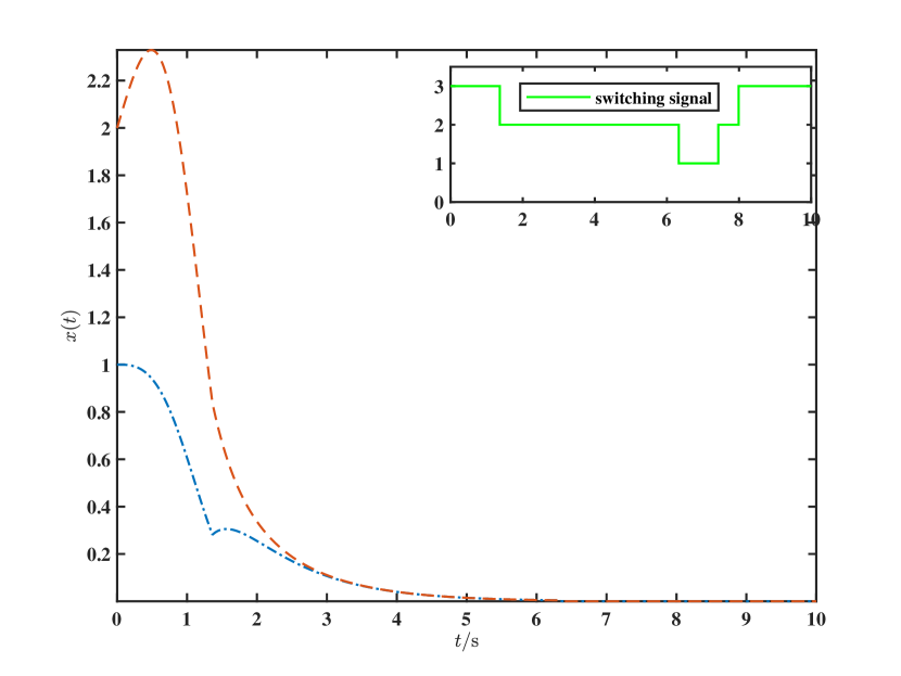
Figure 1: States’ trajectories of system (28) under a single experiment.

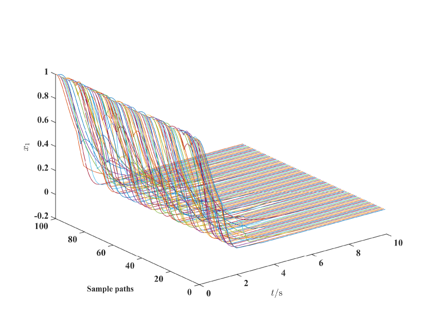
Figure 2: States’ trajectories of system (28) under 100 experiments.

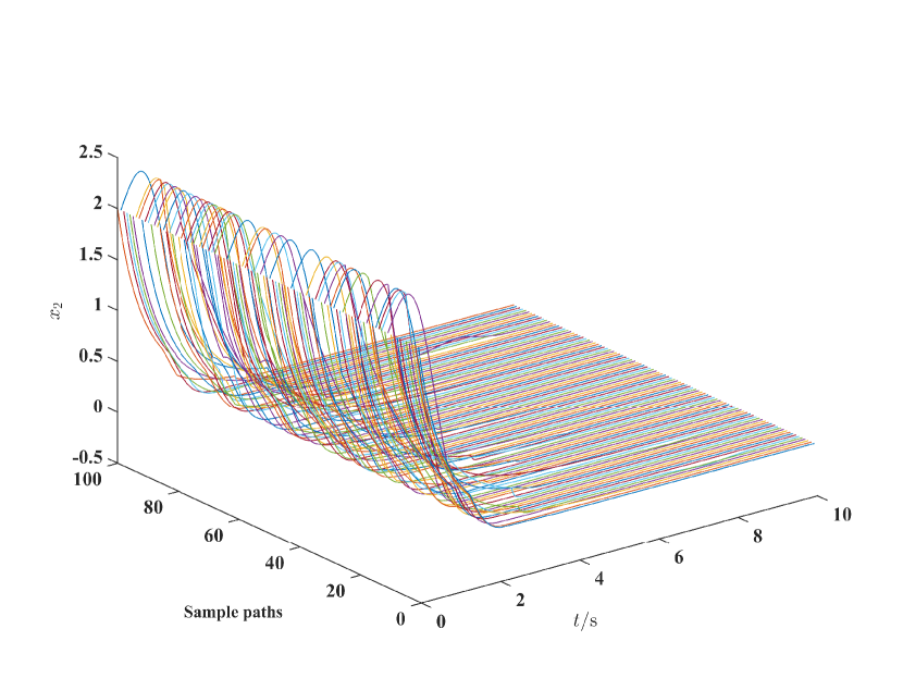
Figure 3: States’ trajectories of system (28) under 100 experiments.

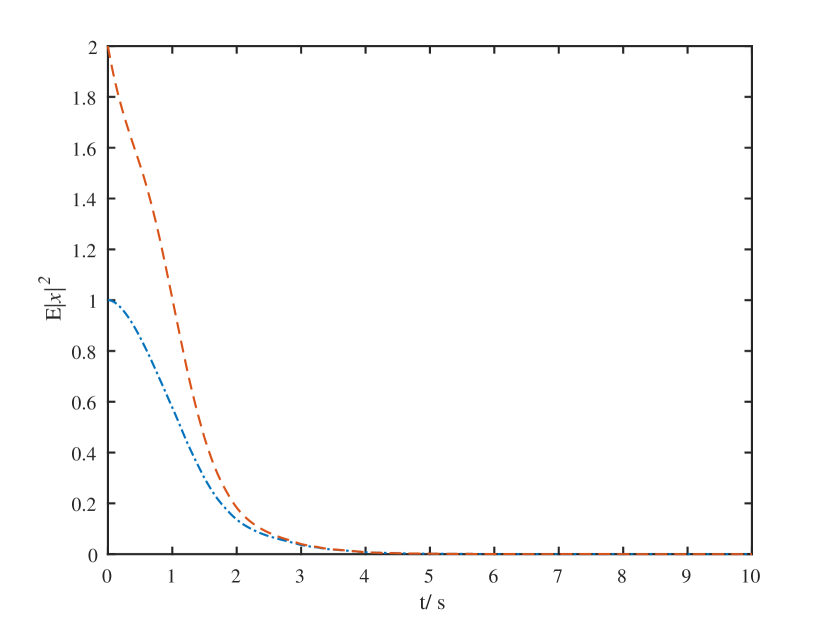
Figure 4: Mean square of states of system (28).

V Conclusion

In this paper, we investigate the stability analysis problem of randomly switched time-varying systems. To get stability criteria, we introduce iMLFs to get stability estimate of each subsystem. Furthermore, novel mean uniformly stable functions are presented, which relax the requirement for uniform stability estimates of individual systems. By utilizing the ergodicity of randomly switching signals, we derive sufficient conditions for almost sure GUAS and GES for the whole system, even without the promise for each subsystem to be stable. We provide numerical examples to illustrate the effectiveness and advantages of our approach.

References

• [1] X. Mao and C. Yuan, Stochastic differential equations with Markovian switching.   London: Imperial college press, 2006.
• [2] D. Chatterjee and D. Liberzon, “Towards ISS disturbance attenuation for randomly switched systems,” in Proceedings of the 46th IEEE Conference on Decision and Control.   IEEE, 2007, pp. 5612–5617.
• [3] ——, “On stability of randomly switched nonlinear systems,” IEEE Transactions on Automatic Control, vol. 52, no. 12, pp. 2390–2394, 2007.
• [4] ——, “Stabilizing randomly switched systems,” SIAM Journal on Control and Optimization, vol. 49, no. 5, pp. 2008–2031, 2011.
• [5] P. Shi and F. B. Li, “A survey on Markovian jump systems: Modeling and design,” International Journal of Control Automation and Systems, vol. 13, no. 1, pp. 1–16, 2015.
• [6] Y. Guo, W. Lin, and G. Chen, “Stability of switched systems on randomly switching durations with random interaction matrices,” IEEE Transactions on Automatic Control, vol. 63, no. 1, pp. 21–36, 2018.
• [7] B. Zhou and W. W. Luo, “Improved Razumikhin and Krasovskii stability criteria for time-varying stochastic time-delay systems,” Automatica, vol. 89, pp. 382–391, 2018.
• [8] N. N. Krasovski, Stability of motion: applications of Lyapunov’s second method to differential systems and equations with delay.   California: Stanford University Press, 1963.
• [9] H. J. Wu and J. T. Sun, “$p$-moment stability of stochastic differential equations with impulsive jump and Markovian switching,” Automatica, vol. 42, no. 10, pp. 1753–1759, 2006.
• [10] S. G. Peng and B. G. Jia, “Some criteria on $p$th moment stability of impulsive stochastic functional differential equations,” Statistics & Probability Letters, vol. 80, no. 13-14, pp. 1085–1092, 2010.
• [11] S. Peng and F. Deng, “New criteria on $p$th moment input-to-state stability of impulsive stochastic delayed differential systems,” IEEE Transactions on Automatic Control, vol. 62, no. 7, pp. 3573–3579, 2017.
• [12] S. G. Peng and Y. Zhang, “Some new criteria on $p$th moment stability of stochastic functional differential equations with Markovian switching,” IEEE Transactions on Automatic Control, vol. 55, no. 12, pp. 2886–2890, 2010.
• [13] C. Y. Ning, Y. He, M. Wu, Q. P. Liu, and J. H. She, “Input-to-state stability of nonlinear systems based on an indefinite Lyapunov function,” Systems & Control Letters, vol. 61, no. 12, pp. 1254–1259, 2012.
• [14] C. Y. Ning, Y. He, M. Wu, and J. H. She, “Improved Razumikhin-type theorem for input-to-state stability of nonlinear time-delay systems,” IEEE Transactions on Automatic Control, vol. 59, no. 7, pp. 1983–1988, 2014.
• [15] C. Y. Ning, Y. He, M. Wu, and S. W. Zhou, “Indefinite derivative Lyapunov-Krasovskii functional method for input to state stability of nonlinear systems with time-delay,” Applied Mathematics and Computation, vol. 270, pp. 534–542, 2015.
• [16] C. Ning, Y. He, M. Wu, and S. Zhou, “Indefinite Lyapunov functions for input-to-state stability of impulsive systems,” Information Sciences, vol. 436, pp. 343–351, 2018.
• [17] B. Zhou and A. V. Egorov, “Razumikhin and Krasovskii stability theorems for time-varying time-delay systems,” Automatica, vol. 71, pp. 281–291, 2016.
• [18] B. Zhou, “Stability analysis of non-linear time-varying systems by Lyapunov functions with indefinite derivatives,” IET Control Theory and Applications, vol. 11, no. 9, pp. 1434–1442, 2017.
• [19] M. Branicky, “Multiple Lyapunov functions and other analysis tools for switched and hybrid systems,” IEEE Transactions on Automatic Control, vol. 43, no. 4, pp. 475–482, APR 1998.
• [20] Z. She and B. Xue, “Discovering multiple Lyapunov functions for switched hybrid systems,” SIAM Journal on Control and Optimization, vol. 52, no. 5, pp. 3312–3340, 2014.
• [21] J. Leth, H. Schioler, M. Gholami, and V. Cocquempot, “Stochastic stability of Markovianly switched systems,” IEEE Transactions on Automatic Control, vol. 58, no. 8, pp. 2048–2054, 2013.
• [22] H. Schioler, M. Simonsen, and J. Leth, “Stochastic stability of systems with semi-Markovian switching,” Automatica, vol. 50, no. 11, pp. 2961–2964, 2014.
• [23] B. Wang and Q. X. Zhu, “Stability analysis of semi-Markov switched stochastic systems,” Automatica, vol. 94, pp. 72–80, 2018.
• [24] J. Lu, Z. She, W. Feng, and S. S. Ge, “Stabilizability of time-varying switched systems based on piecewise continuous scalar functions,” IEEE Transactions on Automatic Control, vol. 64, no. 6, pp. 2637–2644, 2018.
• [25] L. Long, “Integral iss for switched nonlinear time-varying systems using indefinite multiple Lyapunov functions,” IEEE Transactions on Automatic Control, vol. 64, no. 1, pp. 404–411, 2019.
• [26] M. Zhang and Q. Zhu, “New criteria of input-to-state stability for nonlinear switched stochastic delayed systems with asynchronous switching,” Systems & Control Letters, vol. 129, pp. 43–50, 2019.
• [27] S. Chen, C. Ning, Q. Liu, and Q. Liu, “Improved multiple Lyapunov functions of input-output-to-state stability for nonlinear switched systems,” Information Sciences, vol. 608, pp. 47–62, 2022.
• [28] Q. Liu, Y. He, and C. Ning, “Indefinite multiple Lyapunov functions of $p$th moment input-to-state stability and $p$th moment integral input-to-state stability for the nonlinear time-varying stochastic systems with Markovian switching,” International Journal of Robust and Nonlinear Control, vol. 31, no. 11, pp. 5343–5359, 2021.
• [29] ——, “Improved time-varying Halanay inequality with impulses and its application to stability analysis of time-varying semi-Markov switched systems with time-delays,” International Journal of Systems Science, pp. 1–13, 2023.
• [30] G. Chen and Y. Yang, “Relaxed conditions for the input-to-state stability of switched nonlinear time-varying systems,” IEEE Transactions on Automatic Control, vol. 62, no. 9, pp. 4706–4712, 2017.
• [31] X. Wu, Y. Tang, J. Cao, and X. Mao, “Stability analysis for continuous-time switched systems with stochastic switching signals,” IEEE Transactions on Automatic Control, vol. 63, no. 9, pp. 3083–3090, 2019.
• [32] V. S. Barbu and N. Limnios, Semi-Markov chains and hidden semi-Markov models toward applications: their use in reliability and DNA analysis.   Springer Science & Business Media, 2009, vol. 191.