Nonparametric Estimation via Variance-Reduced Sketching

Abstract

Nonparametric models are of great interest in various scientific and engineering disciplines. Classical kernel methods, while numerically robust and statistically sound in low-dimensional settings, become inadequate in higher-dimensional settings due to the curse of dimensionality. In this paper, we introduce a new framework called Variance-Reduced Sketching (VRS), specifically designed to estimate density functions and nonparametric regression functions in higher dimensions with a reduced curse of dimensionality. Our framework conceptualizes multivariable functions as infinite-size matrices, and facilitates a new sketching technique motivated by numerical linear algebra literature to reduce the variance in estimation problems. We demonstrate the robust numerical performance of VRS through a series of simulated experiments and real-world data applications. Notably, VRS shows remarkable improvement over existing neural network estimators and classical kernel methods in numerous density estimation and nonparametric regression models. Additionally, we offer theoretical justifications for VRS to support its ability to deliver nonparametric estimation with a reduced curse of dimensionality.

1 Introduction

Nonparametric models have extensive applications across diverse fields, including biology (MacFarland et al. (2016)), economics (Ullah and Pagan (1999); Li and Racine (2023)), engineering (Lanzante (1996)), and machine learning (Hofmann et al. (2008); Schmidt-hieber (2020)). The most representative nonparametric approaches are kernel methods, known for their numerical robustness and statistical stability in lower-dimensional settings. However, kernel methods often suffer from the curse of dimensionality in higher-dimensional spaces. Recently, a number of significant studies have tackled various modern challenges in nonparametric models. For example, Ravikumar et al. (2009), Raskutti et al. (2012), and Yuan and Zhou (2016) have studied additive models for high-dimensional nonparametric regression; Zhang et al. (2015) and Yang et al. (2017) analyzed randomized algorithms for kernel regression estimation; and Liu et al. (2007) explored nonparametric density estimation in higher dimensions. Despite these contributions, the curse of dimensionality in nonparametric problems, particularly in aspects of statistical accuracy and computational efficiency, remains an open area for further exploration. In this paper, we aim to develop a new framework specifically designed for nonparametric estimation problems. Within this framework, we conceptualize functions as matrices or tensors and explore new methods for handling the bias-variance trade-off, aiming to reduce the curse of dimensionality in higher dimensions.

Matrix approximation algorithms, such as singular value decomposition and QR decomposition, play a crucial role in computational mathematics and statistics. A notable advancement in this area is the emergence of randomized low-rank approximation algorithms. These algorithms excel in reducing time and space complexity substantially without sacrificing too much numerical accuracy. Seminal contributions to this area are outlined in works such as Liberty et al. (2007) and Halko et al. (2011). Additionally, review papers like Woodruff et al. (2014), Drineas and Mahoney (2016), Martinsson (2019), and Martinsson and Tropp (2020) have provided comprehensive summaries of these randomized approaches, along with their theoretical stability guarantees. Randomized low-rank approximation algorithms typically start by estimating the range of a large low-rank matrix $A\in\mathbb{R}^{n\times n}$ by forming a reduced-size sketch. This is achieved by right multiplying $A$ with a random matrix $S\in\mathbb{R}^{n\times k}$, where $k\ll n$. The random matrix $S$ is selected to ensure that the range of $AS$ remains a close approximation of the range of $A$, even when the column size of $AS$ is significantly reduced from $A$. As such, the random matrix $S$ is referred to as randomized linear embedding or sketching matrix by Tropp et al. (2017b) and Nakatsukasa and Tropp (2021). The sketching approach reduces the cost in singular value decomposition from $\operatorname*{O}(n^{3})$ to $\operatorname*{O}(n^{2})$, where $\operatorname*{O}(n^{2})$ represents the complexity of matrix multiplication.

Recently, a series of studies have extended the matrix sketching technique to range estimation for high-order tensor structures, such as the Tucker structure (Che and Wei (2019); Sun et al. (2020); Minster et al. (2020)) and the tensor train structure (Al Daas et al. (2023); Kressner et al. (2023); Shi et al. (2023)). These studies developed specialized structures for sketching to reduce computational complexity while maintaining high levels of numerical accuracy in handling high-order tensors.

Our goal in this paper is to develop a new sketching framework tailored to nonparametric estimation problems. Within this framework, multivariable functions are conceptualized as infinite-size matrices or tensors. In nonparametric estimation contexts, such as density estimation and nonparametric regression, the observed data are discrete samples from the multivariable population functions. Therefore, an additional step of generating matrices or tensors in function space becomes necessary. This process introduces a curse of dimensionality due to the randomness in sampling. Consequently, the task of constructing an appropriate sketching matrix in function spaces that effectively reduces this curse of dimensionality while maintaining satisfactory numerical accuracy in range estimation, poses a significant and intricate challenge.

Previous work has explored randomized sketching techniques in specific nonparametric estimation problems. For instance, Mahoney et al. (2011) and Raskutti and Mahoney (2016) utilized randomized sketching to solve unconstrained least squares problems. Williams and Seeger (2000) , Rahimi and Recht (2007), Kumar et al. (2012) and Tropp et al. (2017a) improved Nyström method with randomized sketching techniques. Similarly, Alaoui and Mahoney (2015), Wang et al. (2017), and Yang et al. (2017) applied randomized sketching to kernel matrices in kernel ridge regression to reduce computational complexity. While these studies mark significant progress in the literature, they usually require extensive observation of the estimated function prior to employing the randomized sketching technique, in order to maintain acceptable accuracy. This step would be significantly expensive for the higher-dimensional setting. Notably, Hur et al. (2023) and subsequent studies Tang et al. (2022); Peng et al. (2023); Chen and Khoo (2023); Tang and Ying (2023) addressed the issues by taking the variance of data generation process into the creation of sketching for high-dimensional tensor estimation. This sketching technique allows for the direct estimation of the range of a tensor with reduced sample complexity in finite dimensions, rather than dealing with the full tensor.

1.1 Contributions

Motivated by Hur et al. (2023), we propose a comprehensive matrix-based sketching framework for estimating multivariate functions in nonparametric models, which we refer to as Variance-Reduced Sketching (VRS). VRS begins by conceptualizing multivariable functions as matrices/tensors and employs a novel sketching technique in functional spaces to estimate the range of the underlying multivariable function. The sketching operators are selected to align with the regularity of the population function and take the randomness of the data generation process into consideration, aiming to reduce variance error in range estimation and the curse of dimensionality in higher-dimensional spaces. Following this, the range estimators are used to estimate the low-rank matrix/tensor representation of the multivariable function. A comprehensive discussion on how to treat multivariable functions as infinite-dimensional matrices and the definition of the corresponding range spaces is provided in Theorem 1. We briefly summarize our contributions as follows:

• In Section 2, we conceptualize multivariable functions as infinite-dimensional matrices and develop new matrix sketching techniques in functional spaces. Our sketching operators in function spaces can be derived from popular statistical nonparametric methods including reproducing kernel Hilbert space basis functions, Legendre polynomial basis functions, and spline basis functions. Our sketching approach takes the variance of random samples in nonparametric models into consideration, providing range estimation of the unknown population function with a reduced curse of dimensionality.

• In Section 3, we develop a general tensor-based nonparametric estimation framework in multivariable function spaces, utilizing the range estimators developed in Section 2. We provide theoretical verification for VRS to justify that the curse of dimensionality of the VRS estimator is greatly reduced. In Section 4, we apply VRS to various nonparametric problems, including density estimation, nonparametric regression, and principle component analysis (PCA) in the continuum limit, aimed to demonstrate the broad applicability of our framework.

• We demonstrate the robust numerical performance of our Variance-Reduced Sketching (VRS) framework through a series of simulated experiments and real data examples. In Figure 1, we conduct simulation studies on density estimation models and nonparametric regression models to compare deep neural network estimators, classical kernel estimators, and VRS. More numerical analysis comparing these methods is provided in Section 5. Extensive numerical evidence indicates that VRS significantly outperforms deep neural network estimators and various classical kernel methods by a considerable margin.

  

  

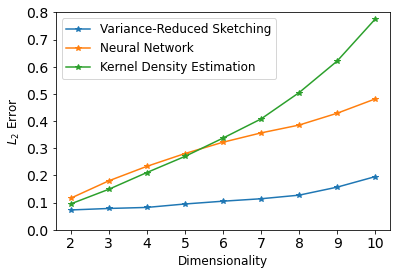
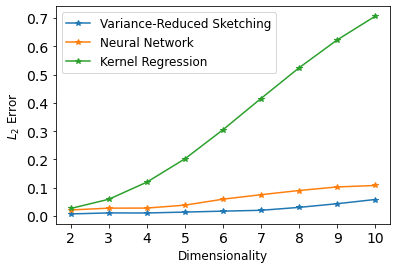
  Figure 1: The left plot corresponds to the density estimation models with the density $p^{*}(x_{1},\ldots,x_{d})\propto\sin\big{(}\frac{\pi}{d}(\sum_{j=1}^{d}x_{j})+\frac{\pi}{4}\big{)}+1$ for $(x_{1},\ldots,x_{d})\in[-1,1]^{d}$. Here $d$ is varied from $2$ to $10$ and the performance of estimators is evaluated using ${{\bf L}_{2}}$-errors. Additional details are provided in Simulation $\mathbf{I}$ of Section 5. The right plot corresponds to the nonparametric regression models with the regression function $f^{*}(x_{1},\ldots,x_{d})=\sin\big{(}\sum_{j=1}^{d}x_{j}\big{)}$ for $(x_{1},\ldots,x_{d})\in[-1,1]^{d}$. Here $d$ is varied from $2$ to $10$ and the performance of estimators is evaluated using ${{\bf L}_{2}}$-errors. Additional details are provided in Simulation $\mathbf{III}$ of Section 5.

1.2 Notations

We use $\mathbb{N}$ to denote the natural numbers $\{1,2,3,\ldots\}$ and $\mathbb{R}$ to denote all the real numbers. We say that $X_{n}=\operatorname*{O_{\mathbb{P}}}(a_{n})$ if for any given $\epsilon>0$, there exists a $K_{\epsilon}>0$ such that

$$\limsup_{n\to\infty}\mathbb{P}(|X_{n}/a_{n}|\geq K_{\epsilon})<\epsilon.$$

For real numbers $\{a_{n}\}_{n=1}$, $\{b_{n}\}_{n=1}$ and $\{c_{n}\}_{n=1}$, we denote $a_{n}=\operatorname*{O}(b_{n})$ if $\lim_{n\to\infty}a_{n}/b_{n}<\infty$ and $a_{n}=\operatorname*{o}(c_{n})$ if $\lim_{n\to\infty}a_{n}/c_{n}=0$. Let $[0,1]$ denote the unit interval in $\mathbb{R}$. For positive integer $d$, denote $\underbrace{[0,1]\times\cdots\times[0,1]}_{d\text{ copies}}=[0,1]^{d}.$

Let $\{f_{i}\}_{i=1}^{n}$ be a collection of elements in the Hilbert space ${\mathcal{H}}$. Then

$$\operatorname*{Span}\{f_{i}\}_{i=1}^{n}=\{b_{1}f_{1}+\cdots+b_{n}f_{n}:\{b_{i}\}_{i=1}^{n}\subset\mathbb{R}\}.$$ (1)

Note that $\operatorname*{Span}\{f_{i}\}_{i=1}^{n}$ is a linear subspace of ${\mathcal{H}}$. Suppose the Hilbert space ${\mathcal{H}}$ is equipped with the norm $\|\cdot\|_{{\mathcal{H}}}$ and $\delta>0$. We say that $\{f_{i}\}_{i=1}^{n}$ is a $\delta$-cover of $\mathcal{G}\subset{\mathcal{H}}$ if for any element $g\in\mathcal{G}$, it holds that $\min_{i=1,\ldots,n}\|g-f_{i}\|_{\mathcal{H}}\leq\delta.$

For a generic measurable set $\Omega\subset\mathbb{R}^{d}$, denote ${{\bf L}_{2}}(\Omega)=\big{\{}f:\Omega\to\mathbb{R}:\|f\|^{2}_{{{\bf L}_{2}}(\Omega)}=\int_{\Omega}f^{2}(z)\mathrm{d}z<\infty\big{\}}.$ For any $f,g\in{{\bf L}_{2}}(\Omega)$, let the inner product between $f$ and $g$ be

$$\langle f,g\rangle=\int_{\Omega}f(z)g(z)\mathrm{d}z.$$

We say that $\{\phi_{k}\}_{k=1}^{\infty}$ is a collection of orthonormal functions in ${{\bf L}_{2}}(\Omega)$ if

$$\langle\phi_{k},\phi_{l}\rangle=\begin{cases}1&\text{if }k=l,\\ 0&\text{if }k\not=l.\end{cases}$$

If in addition that $\{\phi_{k}\}_{k=1}^{\infty}$ spans ${{\bf L}_{2}}(\Omega)$, then $\{\phi_{k}\}_{k=1}^{\infty}$ is a collection of orthonormal basis functions in ${{\bf L}_{2}}(\Omega)$.

In what follows, we briefly introduce the notations for Sobolev spaces. Let $\Omega\subset\mathbb{R}^{d}$ be any measurable set. For multi-index $\beta=(\beta_{1},\ldots,\beta_{d})\in\mathbb{N}^{d}$, and $f(z_{1},\ldots,z_{d}):\Omega\to\mathbb{R}$, define the $\beta$-derivative of $f$ as

$$D^{\beta}f=\partial^{\beta_{1}}_{1}\cdots\partial^{\beta_{d}}_{d}f.$$

Then

$$W^{\alpha}_{2}(\Omega):=\{f\in{{\bf L}_{2}}(\Omega):\ D^{\beta}f\in{{\bf L}_{2}}(\Omega)\text{ for all }|\beta|\leq\alpha\},$$

where $|\beta|=\beta_{1}+\cdots+\beta_{d}$ and $\alpha$ represents the total order of derivatives. The Sobolev norm of $f\in W^{\alpha}_{2}$ is

$$\|f\|_{W^{\alpha}_{2}(\Omega)}^{2}=\sum_{0\leq|\beta|\leq\alpha}\|D^{\beta}f\|_{{{\bf L}_{2}}(\Omega)}^{2}.$$

1.3 Background: linear algebra in function spaces

In what follows, we provide a brief introduction to linear algebra in function spaces. This is the necessary setup to develop our Variance-Reduced Sketching (VRS) framework in nonparametric estimation problems.

Mutivariable functions as matrices

We start with a classical result in functional analysis that allows us to conceptualize mutivariable functions as infinite-dimensional matrices. Let $d_{1}$ and $d_{2}$ be arbitrary positive integers, and let $\Omega_{1}\subset\mathbb{R}^{d_{1}}$ and $\Omega_{2}\subset\mathbb{R}^{d_{2}}$ be two measurable sets.

Theorem 1.

[Singular value decomposition in function space] Let $A(x,y):\Omega_{1}\times\Omega_{2}\to\mathbb{R}$ be any function such that $\|A\|_{{{\bf L}_{2}}(\Omega_{1}\times\Omega_{2})}<\infty$. There exists a collection of strictly positive singular values $\{\sigma_{\rho}(A)\}_{{\rho}=1}^{r}\in\mathbb{R}^{+}$, and two collections of orthonormal basis functions $\{\Phi_{\rho}(x)\}_{{\rho}=1}^{r}\subset{{\bf L}_{2}}(\Omega_{1})$ and $\{\Psi_{\rho}(y)\}_{{\rho}=1}^{r}\subset{{\bf L}_{2}}(\Omega_{2})$ where $r\in\mathbb{N}\cup\{+\infty\}$ such that

$$A(x,y)=\sum_{{\rho}=1}^{r}\sigma_{{\rho}}(A)\Phi_{\rho}(x)\Psi_{\rho}(y).$$ (2)

By viewing $A(x,y)$ as an infinite-dimensional matrix, it follows that the rank of $A(x,y)$ is $r$ and that

$${\operatorname*{Range}}_{x}(A)=\operatorname*{Span}\{\Phi_{\rho}(x)\}_{{\rho}=1}^{r}\quad\text{and}\quad{\operatorname*{Range}}_{y}(A)=\operatorname*{Span}\{\Psi_{\rho}(y)\}_{{\rho}=1}^{r}.$$ (3)

where the definition of Span can be found in (1). Consequently, the rank of $A(x,y)$ is the same as the dimensionality of $\operatorname*{Range}_{x}(A)$ and $\operatorname*{Range}_{y}(A)$.

Mutivariable functions as tensors

Tensor techniques are extensively applied in functional analysis. Here we briefly introduce how to conceptualize multivariable functions as tensors and outline the definitions of norms in this framework.

Given positive integers $\{s_{j}\}_{j=1}^{d}\in\mathbb{N}$, let $\Omega_{j}\subset\mathbb{R}^{s_{j}}$. Let $A(z_{1},\ldots,z_{d}):\Omega_{1}\times\Omega_{2}\cdots\times\Omega_{d}\to\mathbb{R}$ be any generic multivariate function and $u_{j}(z_{j})\in{{\bf L}_{2}}(\Omega_{j})$ for $j=1,\ldots,d$. Denote

$$A[u_{1},\ldots,u_{d}]=\int_{\Omega_{1}}\ldots\int_{\Omega_{d}}A(z_{1},\ldots,z_{d})u_{1}(z_{1})\cdots u_{d}(z_{d})\mathrm{d}z_{1}\cdots\mathrm{d}z_{d}.$$ (4)

Define the Frobenius norm of $A$ as

$$\|A\|_{F}^{2}=\sum_{k_{1},\ldots,k_{d}=1}^{\infty}A^{2}[\phi_{1,k_{1}},\ldots,\phi_{d,k_{d}}],$$ (5)

where $\{\phi_{j,k_{j}}\}_{k_{j}=1}^{\infty}$ are any orthonormal basis functions of ${{\bf L}_{2}}(\Omega_{j})$. Note that in (5), $\|A\|_{F}$ is independent of the choices of basis functions $\{\phi_{j,k_{j}}\}_{k_{j}=1}^{\infty}$ in ${{\bf L}_{2}}(\Omega_{j})$ for $j=1,\ldots,d$. The operator norm of $A$ is defined as

$$\|A\|_{\operatorname*{op}}=\sup_{\|u_{j}\|_{{{\bf L}_{2}}(\Omega_{j})}\leq 1,\ j=1,\ldots,d}A[u_{1},\ldots,u_{d}].$$ (6)

It is well-known from classical functional analysis that two functions $A,B\in{{\bf L}_{2}}(\Omega_{1}\times\Omega_{2}\cdots\times\Omega_{d})$ are equal if and only if $A[u_{1},\ldots,u_{d}]=B[u_{1},\ldots,u_{d}]$ for any set of functions $u_{1}(z_{1})\in{{\bf L}_{2}}(\Omega_{1}),\ldots,u_{d}(z_{d})\in{{\bf L}_{2}}(\Omega_{d})$.

We say that $B$ is a tensor in tensor product space ${{\bf L}_{2}}(\Omega_{1})\otimes{{\bf L}_{2}}(\Omega_{2})\otimes\cdots\otimes{{\bf L}_{2}}(\Omega_{d})$ if there exist scalars $\{b_{k_{1},\ldots,k_{d}}\}_{k_{1},\ldots,k_{d}=1}^{\infty}\subset\mathbb{R}$ and functions $\{f_{j,k_{j}}\}_{k_{j}=1}^{\infty}\subset{{\bf L}_{2}}(\Omega_{j})$ for each $j=1,\ldots,d$ such that

$$A(z_{1},\ldots,z_{d})=\sum_{k_{1},\ldots,k_{d}=1}^{\infty}b_{k_{1},\ldots,k_{d}}f_{1,k_{1}}(z_{1})\cdots f_{d,k_{d}}(z_{d})$$

and that $\|A\|_{F}<\infty$. In other words, ${{\bf L}_{2}}(\Omega_{1})\otimes{{\bf L}_{2}}(\Omega_{2})\cdots\otimes{{\bf L}_{2}}(\Omega_{d})$ is the closure of

$$\operatorname*{Span}\big{\{}f_{1}(z_{1})f_{2}(z_{2})\cdots f_{d}(z_{d}):f_{j}(z_{j})\in{{\bf L}_{2}}(\Omega_{j})\text{ for all }j=1,\ldots,d\big{\}}.$$

From classical functional analysis, we have that

$${{\bf L}_{2}}(\Omega_{1})\otimes{{\bf L}_{2}}(\Omega_{2})\cdots\otimes{{\bf L}_{2}}(\Omega_{d})={{\bf L}_{2}}(\Omega_{1}\times\Omega_{2}\cdots\times\Omega_{d})\quad\text{and}\quad\|A\|_{{{\bf L}_{2}}(\Omega_{1}\times\cdots\times\Omega_{d})}=\|A\|_{F}.$$ (7)

Projection operators in function spaces

Finally, we offer a brief overview of projection operators and its applications to tensors in function spaces. Let $\mathcal{U}=\text{span}\{\phi_{1},\ldots,\phi_{m}\}\subset{{\bf L}_{2}}(\Omega)$, where $m\in\mathbb{N}$ and $\{\phi_{{\mu}}\}_{{\mu}=1}^{m}$ are any orthonormal functions. Then $\mathcal{U}$ is an $m$-dimensional linear subspace of ${{\bf L}_{2}}(\Omega)$ and we denote $\dim(\mathcal{U})=m$. Let $\mathcal{P}_{\mathcal{U}}$ be the projection operator onto the subspace $\mathcal{U}$. Formally, we can write $\mathcal{P}_{\mathcal{U}}=\sum_{{\mu}=1}^{m}\phi_{{\mu}}\otimes\phi_{{\mu}}\in{{\bf L}_{2}}(\Omega)\otimes{{\bf L}_{2}}(\Omega)$. Therefore for any $f\in{{\bf L}_{2}}(\Omega)$, the projection of $f$ on $\mathcal{U}$ is

$$\mathcal{P}_{\mathcal{U}}(f)=\sum_{{\mu}=1}^{m}\langle f,\phi_{{\mu}}\rangle\phi_{{\mu}}.$$ (8)

Note that by definition, we always have $\|\mathcal{P}_{\mathcal{U}}\|_{\operatorname*{op}}\leq 1$ for any projection operator $\mathcal{P}_{\mathcal{U}}$.

For $j=1,\ldots,d$, let $\{\phi_{j,{{\mu}}_{j}}\}_{{{\mu}}_{j}=1}^{\infty}$ be any orthonormal basis functions of ${{\bf L}_{2}}(\Omega_{j})$, and

$$\mathcal{U}_{j}=\text{span}\{\phi_{j,{{\mu}}_{j}}\}_{{{\mu}}_{j}=1}^{{m}_{j}},$$ (9)

where ${m}_{j}\in\mathbb{N}$. Define the tensor $A\times_{1}\mathcal{P}_{\mathcal{U}_{1}}\cdots\times_{d}\mathcal{P}_{\mathcal{U}_{d}}$ as

$$\left(A\times_{1}\mathcal{P}_{\mathcal{U}_{1}}\cdots\times_{d}\mathcal{P}_{\mathcal{U}_{d}}\right)[u_{1},\ldots,u_{d}]=A[\mathcal{P}_{\mathcal{U}_{1}}(u_{1}),\ldots,\mathcal{P}_{\mathcal{U}_{d}}(u_{d})]$$ (10)

for any $u_{1}\in{{\bf L}_{2}}(\Omega_{1}),\ldots,u_{d}\in{{\bf L}_{2}}(\Omega_{d})$. By Lemma 18,

$$\|A\times_{1}\mathcal{P}_{\mathcal{U}_{1}}\cdots\times_{d}\mathcal{P}_{\mathcal{U}_{d}}\|_{F}\leq\|A\|_{F}\|\mathcal{P}_{\mathcal{U}_{1}}\|_{\operatorname*{op}}\cdots\|\mathcal{P}_{\mathcal{U}_{d}}\|_{\operatorname*{op}}=\|A\|_{F}<\infty.$$

It follows that $A\times_{1}\mathcal{P}_{\mathcal{U}_{1}}\cdots\times_{d}\mathcal{P}_{\mathcal{U}_{d}}$ is a tensor in ${{\bf L}_{2}}(\Omega_{1})\otimes{{\bf L}_{2}}(\Omega_{2})\otimes\cdots\otimes{{\bf L}_{2}}(\Omega_{d})$ and therefore can be viewed as a function in ${{\bf L}_{2}}(\Omega_{1}\times\Omega_{2}\cdots\times\Omega_{d})$ and the corresponding function expression can be found in Lemma 19 in the appendix.

More generally given $k\leq d$, let $x=(z_{1},\ldots,z_{k})\in\Omega_{1}\times\cdots\times\Omega_{k}$ and $y=(z_{k+1},\ldots,z_{d})\in\Omega_{k+1}\times\cdots\times\Omega_{d}$. We can view $A(z_{1},\ldots,z_{d})=A(x,y)$ as an infinitely-dimensional matrix in ${{\bf L}_{2}}(\Omega_{1}\times\cdots\times\Omega_{k})\otimes{{\bf L}_{2}}(\Omega_{k+1}\times\cdots\times\Omega_{d})$. For $j=1,\ldots,k$, let $\mathcal{U}_{j}\subset{{\bf L}_{2}}(\Omega_{j})\$ be defined as in (9). Suppose $\mathcal{U}_{x}\subset{{\bf L}_{2}}(\Omega_{1}\times\cdots\times\Omega_{k})$ is such that

$$\mathcal{U}_{x}=\mathcal{U}_{1}\otimes\cdots\otimes\mathcal{U}_{k}=\operatorname*{Span}\{f_{1}(z_{1})\cdots f_{k}(z_{k}),\ f_{j}(z_{j})\in\mathcal{U}_{j}\text{ for all }1\leq j\leq k\}.$$

Then we have $A\times_{x}\mathcal{P}_{\mathcal{U}_{x}}=A\times_{1}\mathcal{P}_{\mathcal{U}_{1}}\cdots\times_{k}\mathcal{P}_{\mathcal{U}_{k}},$ as shown in Lemma 20.

2 Range estimation by sketching

Let $d_{1}$ and $d_{2}$ be arbitrary positive integers, and let $\Omega_{1}\subset\mathbb{R}^{d_{1}}$ and $\Omega_{2}\subset\mathbb{R}^{d_{2}}$ be two measurable sets. Let $A^{*}(x,y):\Omega_{1}\times\Omega_{2}\to\mathbb{R}$ be the unknown population function, and suppose $\widehat{A}$ is the sample version of $A^{*}$ formed by the observed data. In this section, we introduce the main algorithm to estimate $\operatorname*{Range}_{x}(A^{*})$ with a reduced curse of dimensionality when $A^{*}$ is treated as an infinite-dimensional matrix by Theorem 1. To this end, let $\mathcal{M}$ be a linear subspace of ${{\bf L}_{2}}(\Omega_{1})$ that acts as an estimation subspace and $\mathcal{L}$ be a linear subspace of ${{\bf L}_{2}}(\Omega_{2})$ that acts as a sketching subspace. More details on how to choose $\mathcal{M}$ and $\mathcal{L}$ are deferred to Remark 2. Our procedure is composed of the following three stages.

• Sketching stage. Let $\{w_{{\eta}}\}_{{\eta}=1}^{\dim(\mathcal{L})}$ be the orthonormal basis functions of $\mathcal{L}$. We apply the projection operator $\mathcal{P}_{\mathcal{L}}$ to $\widehat{A}$ by computing

  $$\bigg{\{}\int_{\Omega_{2}}\widehat{A}(x,y)w_{{\eta}}(y)\mathrm{d}y\bigg{\}}_{{\eta}=1}^{\dim(\mathcal{L})}.$$ (11)

  Note that for each ${\eta}=1,\ldots,\dim(\mathcal{L})$, $\int_{\Omega_{2}}\widehat{A}(x,y)w_{{\eta}}(y)\mathrm{d}y$ is a function solely depending on $x$. This stage is aiming at reducing the curse of dimensionality associated to variable $y$.

• Estimation stage. We estimate the functions $\big{\{}\int_{\Omega_{2}}\widehat{A}(x,y)w_{{\eta}}(y)\mathrm{d}y\big{\}}_{{\eta}=1}^{\text{dim}(\mathcal{L})}$ by utilizing the estimation space $\mathcal{M}$. Specifically, for each ${\eta}=1,\ldots,\dim(\mathcal{L})$, we approximate $\int_{\Omega_{2}}\widehat{A}(x,y)w_{{\eta}}(y)\mathrm{d}y$ by

  $$\widetilde{f}_{\eta}(x)=\operatorname*{arg\,min}_{f\in\mathcal{M}}\bigg{\|}\int_{\Omega_{2}}\widehat{A}(x,y)w_{{\eta}}(y)\mathrm{d}y-f(x)\bigg{\|}^{2}_{{{\bf L}_{2}}(\Omega_{1})}.$$ (12)

• Orthogonalization stage. Let

  $$\widetilde{A}(x,y)=\sum_{{\eta}=1}^{\dim(\mathcal{L})}\widetilde{f}_{\eta}(x)w_{\eta}(y).$$ (13)

  Compute the leading singular functions in the variable $x$ of $\widetilde{A}(x,y)$ to estimate the $\operatorname*{Range}_{x}(A^{*})$.

We formally summarize our procedure in Algorithm 1.

1:Estimator $\widehat{A}(x,y):\Omega_{1}\times\Omega_{2}\to\mathbb{R}$, parameter $r\in\mathbb{Z}^{+}$, linear subspaces $\mathcal{M}\subset{{\bf L}_{2}}(\Omega_{1})$ and $\mathcal{L}\subset{{\bf L}_{2}}(\Omega_{2})$.

2:Compute $\big{\{}\int_{\Omega_{2}}\widehat{A}(x,y)w_{{\eta}}(y)\mathrm{d}y\big{\}}_{{\eta}=1}^{\dim(\mathcal{L})},$ the projection of $\widehat{A}$ onto $\{w_{{\eta}}(y)\}_{{\eta}=1}^{\dim(\mathcal{L})}$, the basis functions of $\mathcal{L}$.

3:Compute the estimated functions $\{\widetilde{f}_{\eta}(x)\}_{{\eta}=1}^{\dim(\mathcal{L})}$ in $\mathcal{M}$ by (12).

4:Compute the leading $r$ singular functions in the variable $x$ of $\widetilde{A}(x,y)=\sum_{{\eta}=1}^{\dim(\mathcal{L})}\widetilde{f}_{\eta}(x)w_{\eta}(y)$ and denote them as $\{\widehat{\Phi}_{\rho}(x)\}_{{\rho}=1}^{r}$.

5:$\{\widehat{\Phi}_{\rho}(x)\}_{{\rho}=1}^{r}$.

Algorithm 1 Range Estimation via Variance-Reduced Sketching

Remark 1.

Assuming that estimation space $\mathcal{M}$ is spanned by the orthonormal basis functions $\{v_{{\mu}}(x)\}_{{\mu}=1}^{\dim(\mathcal{M})}$. In what follows, we provide an explicit expression of $\widetilde{A}(x,y)$ in (13) based on the $\widehat{A}(x,y)$.

In the sketching stage, computing (11) is equivalent to compute $\widehat{A}\times_{y}\mathcal{P}_{\mathcal{L}}$, as

$$\widehat{A}\times_{y}\mathcal{P}_{\mathcal{L}}=\sum_{{\eta}=1}^{\dim(\mathcal{L})}\bigg{(}\int_{\Omega_{2}}\widehat{A}(x,y)w_{{\eta}}(y)\mathrm{d}y\bigg{)}w_{{\eta}}(y).$$

In the estimation stage, we have the following explicit expression for (12) by Lemma 22:

$$\widehat{f}_{\eta}(x)=\sum_{{\mu}=1}^{\dim(\mathcal{M})}\widehat{A}[v_{\mu},w_{\eta}]v_{\mu}(x),$$

where $\widehat{A}[v_{\mu},w_{\eta}]=\iint\widehat{A}(x,y)v_{{\mu}}(x)w_{{\eta}}(y)\mathrm{d}x\mathrm{d}y$. Therefore, $\widetilde{A}(x,y)$ in (13) can be rewritten as

$$\widetilde{A}(x,y)=\sum_{{\mu}=1}^{\dim(\mathcal{M})}\sum_{{\eta}=1}^{\dim(\mathcal{L})}\widehat{A}[v_{\mu},w_{\eta}]v_{\mu}(x)w_{\eta}(y).$$ (14)

By Lemma 21, $\widehat{A}\times_{x}\mathcal{P}_{\mathcal{M}}\times_{y}\mathcal{P}_{\mathcal{L}}$ has the exact same expression as $\widetilde{A}$. Therefore, we establish the identification

$$\widetilde{A}=\widehat{A}\times_{x}\mathcal{P}_{\mathcal{M}}\times_{y}\mathcal{P}_{\mathcal{L}}.$$ (15)

In 5 of the appendix, we provide further implementation details on how to compute the leading $r$ singular functions in the variable $x$ of $\widehat{A}\times_{x}\mathcal{P}_{\mathcal{M}}\times_{y}\mathcal{P}_{\mathcal{L}}$ using singular value decomposition. Let ${\mathcal{P}}_{x}^{*}$ be the projection operator onto the $\operatorname*{Range}_{x}(A^{*})$, and let $\widehat{\mathcal{P}}_{x}$ be the projection operator onto the space spanned by $\{\widehat{\Phi}_{\rho}(x)\}_{{\rho}=1}^{r}$, the output of Algorithm 1. In Section 2.2, we show that the range estimator in Algorithm 1 is consistent by providing theoretical quantification on the difference between ${\mathcal{P}}_{x}^{*}$ and $\widehat{\mathcal{P}}_{x}$.

2.1 Intuition in finite-dimensional vector spaces

In this subsection, we illustrate the intuition of sketching in a finite-dimensional matrix example. Suppose $B\in\mathbb{R}^{n_{1}\times n_{2}}$ is a finite-dimensional matrix with rank $r$. Let $\operatorname*{Range}(B)\subset\mathbb{R}^{n_{1}}$ denote the linear subspace spanned by the columns of $B$, and $\text{Row}(B)\subset\mathbb{R}^{n_{2}}$ the linear subspace spanned by the rows of $B$. Our goal is to illustrate how to estimate  $\operatorname*{Range}(B)$ with reduced variance and reduced computational complexity when $n_{1}\ll n_{2}$.

By singular value decomposition, we can write

$$B=\sum_{{\rho}=1}^{r}\sigma_{{\rho}}(B)U_{{\rho}}V_{{\rho}}^{\top},$$

where $\sigma_{1}(B)\geq\cdots\geq\sigma_{r}(B)>0$ are singular values, $\{U_{\rho}\}_{{\rho}=1}^{r}$ are orthonormal vectors in $\mathbb{R}^{n_{1}}$, and $\{V_{\rho}\}_{{\rho}=1}^{r}$ are orthonormal vectors in $\mathbb{R}^{n_{2}}$. Therefore $\operatorname*{Range}(B)$ is spanned by $\{U_{{\rho}}\}_{{\rho}=1}^{r}$, and $\text{Row}(B)$ is spanned by $\{V_{\rho}\}_{{\rho}=1}^{r}$.

The sketch-based estimation procedure of $\operatorname*{Range}(B)$ is as follows. First, we choose a linear subspace $\mathcal{S}\subset\mathbb{R}^{n_{2}}$ such that $\dim(\mathcal{S})\ll n_{2}$ and that $\mathcal{S}$ forms a $\delta$-cover of $\text{Row}(B)$. Let $P_{\mathcal{S}}$ be the projection matrix from $\mathbb{R}^{n_{2}}$ to $\mathcal{S}$ and we form the sketch matrix $BP_{\mathcal{S}}^{\top}\in\mathbb{R}^{n_{1}\times\dim(\mathcal{S})}$. Then in the second stage, we use the singular value decomposition to compute $\operatorname*{Range}(BP_{\mathcal{S}}^{\top})$ and return $\operatorname*{Range}(BP_{\mathcal{S}}^{\top})$ as the estimator of $\operatorname*{Range}(B)$.

With the sketching technique, we only need to work with the reduced-size matrix $BP_{\mathcal{S}}^{\top}\in\mathbb{R}^{n_{1}\times\dim(\mathcal{S})}$ instead of $B\in\mathbb{R}^{n_{1}\times n_{2}}$. Therefore, the effective variance of the sketching procedure is reduced to $\operatorname*{O}(n_{1}\dim(\mathcal{S}))$, significantly smaller than $\operatorname*{O}(n_{1}n_{2})$ which is the cost if we directly use $B$ to estimate the range.

We also provide an intuitive argument to support the above sketching procedure. Since $BP_{\mathcal{S}}^{\top}=\sum_{{\rho}=1}^{r}\sigma_{\rho}(B)U_{\rho}(P_{\mathcal{S}}V_{\rho})^{\top}$, it holds that

$$\operatorname*{Range}(BP_{\mathcal{S}}^{\top})\subset\operatorname*{Range}(B).$$ (16)

Let $\|\cdot\|_{2}$ indicate matrix spectral norm for matrix and vector $l_{2}$ norm. Since the subspace $\mathcal{S}$ is a $\delta$-cover of $\text{Row}(B)$, it follows that $\|P_{\mathcal{S}}V_{\rho}-V_{\rho}\|\leq\delta$ for ${\rho}=1,\ldots,r$. Therefore

$$\|B-BP_{\mathcal{S}}^{\top}\|_{2}=\bigg{\|}\sum_{{\rho}=1}^{r}\sigma_{\rho}(B)U_{\rho}(V_{\rho}-P_{\mathcal{S}}V_{\rho})^{\top}\bigg{\|}_{2}\leq\sum_{{\rho}=1}^{r}|\sigma_{\rho}(B)|\|U_{\rho}\|_{2}\|V_{\rho}-P_{\mathcal{S}}V_{\rho}\|_{2}=\operatorname*{O}(\delta),$$

where the last equality follows from the fact that $|\sigma_{\rho}(B)|<\infty$ and $\|U_{\rho}\|_{2}=1$ for ${\rho}=1,\ldots,r$. Let $\{\sigma_{\rho}(BP_{\mathcal{S}}^{\top})\}_{{\rho}=1}^{r}$ be the leading $r$ singular values of $BP_{\mathcal{S}}^{\top}$. By matrix singular value perturbation theory,

$$|\sigma_{\rho}(B)-\sigma_{\rho}(BP_{\mathcal{S}}^{\top})|\leq\|B-BP_{\mathcal{S}}^{\top}\|_{2}=\operatorname*{O}(\delta).$$ (17)

for ${\rho}=1,\ldots,r$. Suppose $\mathcal{S}$ is chosen so that $\delta\ll\sigma_{r}(B)$, where $\sigma_{r}(B)$ is the minimal singular value of $B$. Then (17) implies that $\sigma_{\rho}(BP_{\mathcal{S}}^{\top})\geq\sigma_{\rho}(B)-\operatorname*{O}(\delta)>0$ for ${\rho}\in\{1,\ldots,r\}$. Therefore, $BP_{\mathcal{S}}^{\top}$ has at least $r$ positive singular values and the rank of $BP_{\mathcal{S}}^{\top}$ is at least $r$. This observation, together with (16) and the fact that $\operatorname*{Rank}(B)=r$ implies that

$$\operatorname*{Range}(BP_{\mathcal{S}}^{\top})=\operatorname*{Range}(B).$$

This justifies the sketching procedure in finite-dimensions.

2.2 Error analysis of Algorithm 1

In this subsection, we study the theoretical guarantees of Algorithm 1. We start with introducing necessary conditions to establish the consistency of our range estimators.

Assumption 1.

Suppose $\Omega_{1}\subset\mathbb{R}^{d_{1}}$ and $\Omega_{2}\subset\mathbb{R}^{d_{2}}$ be two measurable sets. Let $A^{*}(x,y):\Omega_{1}\times\Omega_{2}\to\mathbb{R}$ be a generic population function with $\|A^{*}\|_{{{\bf L}_{2}}(\Omega_{1}\times\Omega_{2})}<\infty$.

$$A^{*}(x,y)=\sum_{{\rho}=1}^{r}\sigma_{{\rho}}\Phi^{*}_{{\rho}}(x)\Psi^{*}_{{\rho}}(y),$$

where $r\in\mathbb{N}$, $\sigma_{1}\geq\sigma_{2}\geq\ldots\geq\sigma_{r}>0$, and $\{\Phi_{{\rho}}^{*}(x)\}_{{\rho}=1}^{r}$ and $\{\Psi^{*}_{{\rho}}(y)\}_{{\rho}=1}^{r}$ are orthonormal basis functions in ${{\bf L}_{2}}(\Omega_{1})$ and ${{\bf L}_{2}}(\Omega_{2})$ respectively.

The finite-rank condition in 1 is commonly observed in the literature. In Example 1 and Example 2 of Appendix B, we illustrate that both additive models in nonparametric regression and mean-field models in density estimation satisfy 1. Additionally, in Example 3, we demonstrate that all multivariable differentiable functions can be effectively approximated by finite-rank functions.

Furthermore, the following assumption quantifies the bias between $A^{*}$ and its projection.

Assumption 2.

Let $\mathcal{M}\subset{{\bf L}_{2}}(\Omega_{1})$ and $\mathcal{L}\subset{{\bf L}_{2}}(\Omega_{2})$ be two linear subspaces such that $\dim(\mathcal{M})=m^{d_{1}}$ and $\dim(\mathcal{L})=\ell^{d_{2}}$, where $m,\ell\in\mathbb{N}$. For $\alpha\geq 1$, suppose that

$$\|A^{*}-A^{*}\times_{x}\mathcal{P}_{\mathcal{M}}\times_{y}\mathcal{P}_{\mathcal{L}}\|^{2}_{{{\bf L}_{2}}(\Omega_{1}\times\Omega_{2})}=\operatorname*{O}(m^{-2\alpha}+\ell^{-2\alpha}),$$ (18)

$$\|A^{*}-A^{*}\times_{y}\mathcal{P}_{\mathcal{L}}\|^{2}_{{{\bf L}_{2}}(\Omega_{1}\times\Omega_{2})}=\operatorname*{O}(\ell^{-2\alpha}),\quad\text{and}$$ (19)

$$\|A^{*}\times_{y}\mathcal{P}_{\mathcal{L}}-A^{*}\times_{x}\mathcal{P}_{\mathcal{M}}\times_{y}\mathcal{P}_{\mathcal{L}}\|^{2}_{{{\bf L}_{2}}(\Omega_{1}\times\Omega_{2})}=\operatorname*{O}(m^{-2\alpha}).$$ (20)

Remark 2.

When $\Omega_{1}=[0,1]^{d_{1}}$ and $\Omega_{2}=[0,1]^{d_{2}}$, 2 directly follows from approximation theories in Sobolev spaces. Indeed in the Appendix A, under the assumption that $\|A^{*}\|_{W^{\alpha}_{2}({[0,1]}^{d_{1}+d_{2}})}<\infty,$ we justify 2 when $\mathcal{M}$ and $\mathcal{L}$ are derived from three different popular nonparametric approaches: the reproducing kernel Hilbert spaces in Lemma 2, the Legendre polynomial system in Lemma 5, and the spline regression in Lemma 7.

Suppose $\widehat{A}$ is formed from data of sample size $N$, the following assumption quantifies the deviation between $\widehat{A}$ and $A^{*}$ within the subspace $\mathcal{M}\otimes\mathcal{L}$.

Assumption 3.

Let $\mathcal{M}\subset{{\bf L}_{2}}(\Omega_{1})$ and $\mathcal{L}\subset{{\bf L}_{2}}(\Omega_{2})$ be two linear subspaces. Suppose that

$$\|(\widehat{A}-A^{*})\times_{x}\mathcal{P}_{\mathcal{M}}\times_{y}\mathcal{P}_{\mathcal{L}}\|_{\operatorname*{op}}=\operatorname*{O_{\mathbb{P}}}\bigg{(}\sqrt{\frac{\dim(\mathcal{M})+\dim(\mathcal{L})}{N}}\bigg{)}.$$ (21)

Remark 3.

3 can be interpreted as a matrix perturbation bound in function spaces. In Section 4, we verify 3 when the data are sampled from three nonparametric models: the density estimation model, the non-parametric regression model, and PCA model.

Note that by the identification in (15), $\widetilde{A}=\widehat{A}\times_{x}\mathcal{P}_{\mathcal{M}}\times_{y}\mathcal{P}_{\mathcal{L}}$. The following theorem shows that $\operatorname*{Range}_{x}(A^{*})$ can be well-approximated by the leading singular functions in $x$ of $\widehat{A}\times_{x}\mathcal{P}_{\mathcal{M}}\times_{y}\mathcal{P}_{\mathcal{L}}$.

Theorem 2.

Suppose 1, 2 and 3 hold. For a sufficiently large constant $C$, suppose that

$$\sigma_{r}>C\max\bigg{\{}\ell^{-\alpha},m^{-\alpha},\sqrt{\frac{m^{d_{1}}+\ell^{d_{2}}}{N}}\bigg{\}}.$$ (22)

Let ${\mathcal{P}}_{x}^{*}$ be the projection operator onto the $\operatorname*{Range}_{x}(A^{*})$, and let $\widehat{\mathcal{P}}_{x}$ be the projection operator onto the space spanned by the leading $r$ singular functions in the variable $x$ of $\widehat{A}\times_{x}\mathcal{P}_{\mathcal{M}}\times_{y}\mathcal{P}_{\mathcal{L}}$. Then

$$\|\widehat{\mathcal{P}}_{x}-\mathcal{P}^{*}_{x}\|_{\operatorname*{op}}^{2}=\operatorname*{O_{\mathbb{P}}}\bigg{\{}\sigma_{r}^{-2}\bigg{(}\frac{m^{d_{1}}+\ell^{d_{2}}}{N}+m^{-2\alpha}\bigg{)}\bigg{\}}.$$ (23)

It follows that if $m\asymp N^{1/(2\alpha+d_{1})}$, $\ell=C_{L}\sigma_{r}^{-1/\alpha}$ for a sufficiently large constant $C_{L}$, and that

$$N\geq C_{\sigma}\max\{\sigma_{r}^{-2-d_{1}/\alpha},\sigma_{r}^{-2-d_{2}/\alpha}\}$$

for a sufficiently large constant $C_{\sigma}$, then Theorem 2 implies that

$$\|\widehat{\mathcal{P}}_{x}-\mathcal{P}^{*}_{x}\|_{\operatorname*{op}}^{2}=\operatorname*{O_{\mathbb{P}}}\bigg{\{}\frac{\sigma_{r}^{-2}}{N^{2\alpha/(2\alpha+d_{1})}}+\frac{\sigma_{r}^{-2-d_{2}/\alpha}}{N}\bigg{\}}.$$ (24)

To interpret our result in Theorem 2, consider a simplified scenario where the minimal spectral value $\sigma_{r}$ is a positive constant. Then (24) further reduces to

$$\|\widehat{\mathcal{P}}_{x}-\mathcal{P}^{*}_{x}\|_{\operatorname*{op}}^{2}=\operatorname*{O_{\mathbb{P}}}\bigg{\{}\frac{1}{N^{2\alpha/(2\alpha+d_{1})}}\bigg{\}},$$

which matches the optimal non-parametric estimation rate in the function space $W^{\alpha}_{2}(\mathbb{R}^{d_{1}})$. This indicates that our method is able to estimate $\operatorname*{Range}_{x}(A^{*})$ without the curse of dimensionality introduced by the variable $y\in\mathbb{R}^{d_{2}}$. Utilizing the estimator of $\mathcal{P}^{*}_{x}$, we can further estimate the population function $A^{*}$ with reduced curse of dimensionality as detailed in Section 3.

An overview of proof of Theorem 2

The proof of Theorem 2 can be found in Section C.1. In what follows, we provide an overview of proof of Theorem 2. To begin, we choose the sketching subspace $\mathcal{L}$ with $\dim(\mathcal{L})=\ell^{d_{2}}$. If $\ell$ chosen so that $\sigma_{r}\geq C{\ell}^{-\alpha}$ for sufficiently large constant $C$, then by (19) of 2, it holds that $\|A^{*}-A^{*}\times_{y}\mathcal{P}_{\mathcal{L}}\|_{\operatorname*{op}}<\sigma_{r}/2.$ It follows from spectral perturbation bound in Hilbert space that $A^{*}\times_{y}\mathcal{P}_{\mathcal{L}}$ has at least $r$ non-zero singular values and so

$${\operatorname*{Range}}_{x}(A^{*}\times_{y}\mathcal{P}_{\mathcal{L}})={\operatorname*{Range}}_{x}(A^{*})$$ (25)

The proof of (25) can be found in Lemma 8 of the appendix. Therefore $\mathcal{P}_{x}^{*}$ is also the range projection operator of $A^{*}\times_{y}\mathcal{P}_{\mathcal{L}}$.

The next step is to apply the Hilbert space Wedin’s theorem (Corollary 8) to $A^{*}\times_{y}\mathcal{P}_{\mathcal{L}}$ and $\widehat{A}\times_{x}\mathcal{P}_{\mathcal{M}}\times_{y}\mathcal{P}_{\mathcal{L}}$ to get

$$\|\mathcal{P}_{x}^{*}-\widehat{\mathcal{P}}_{x}\|_{\operatorname*{op}}\lesssim\frac{\|A^{*}\times_{y}\mathcal{P}_{\mathcal{L}}-\widehat{A}\times_{x}\mathcal{P}_{\mathcal{M}}\times_{y}\mathcal{P}_{\mathcal{L}}\|_{\operatorname*{op}}}{\sigma_{r}-\|A^{*}\times_{y}\mathcal{P}_{\mathcal{L}}-\widehat{A}\times_{x}\mathcal{P}_{\mathcal{M}}\times_{y}\mathcal{P}_{\mathcal{L}}\|_{\operatorname*{op}}}.$$ (26)

It suffices to bound $\|A^{*}\times_{y}\mathcal{P}_{\mathcal{L}}-\widehat{A}\times_{x}\mathcal{P}_{\mathcal{M}}\times_{y}\mathcal{P}_{\mathcal{L}}\|_{\operatorname*{op}}$. By triangle inequality,

$$\|A^{*}\times_{y}\mathcal{P}_{\mathcal{L}}-\widehat{A}\times_{x}\mathcal{P}_{\mathcal{M}}\times_{y}\mathcal{P}_{\mathcal{L}}\|_{\operatorname*{op}}$$

$$\leq \|A^{*}\times_{y}\mathcal{P}_{\mathcal{L}}-A^{*}\times_{x}\mathcal{P}_{\mathcal{M}}\times_{y}\mathcal{P}_{\mathcal{L}}\|_{\operatorname*{op}}$$ (27)

$$+ \|A^{*}\times_{x}\mathcal{P}_{\mathcal{M}}\times_{y}\mathcal{P}_{\mathcal{L}}-\widehat{A}\times_{x}\mathcal{P}_{\mathcal{M}}\times_{y}\mathcal{P}_{\mathcal{L}}\|_{\operatorname*{op}},$$ (28)

where (27) is the bias and (28) is the variance of our estimation procedure. Subsequently, we use (20) in 2 to bound (27) and 3 to bound (28) to get that, with high probability,

$$\|A^{*}\times_{y}\mathcal{P}_{\mathcal{L}}-\widehat{A}\times_{x}\mathcal{P}_{\mathcal{M}}\times_{y}\mathcal{P}_{\mathcal{L}}\|_{\operatorname*{op}}=\operatorname*{O}\bigg{(}\sqrt{\frac{m^{d_{1}}+\ell^{d_{2}}}{N}}+m^{-\alpha}\bigg{)},$$ (29)

where the term $m^{-\alpha}$ corresponds to the bias and the term $\sqrt{\frac{m^{d_{1}}+{\ell}^{d_{2}}}{N}}$ corresponds to the variance of our estimator. With sufficient sample size $N$, we can balance the bias and the variance in (29) to further ensure that $\|A^{*}\times_{y}\mathcal{P}_{\mathcal{L}}-\widehat{A}\times_{x}\mathcal{P}_{\mathcal{M}}\times_{y}\mathcal{P}_{\mathcal{L}}\|_{\operatorname*{op}}=\operatorname*{o}(\sigma_{r})$. Finally, (26) and (29) together imply that

$$\|\mathcal{P}_{x}^{*}-\widehat{\mathcal{P}}_{x}\|_{\operatorname*{op}}\lesssim\frac{\|A^{*}\times_{y}\mathcal{P}_{\mathcal{L}}-\widehat{A}\times_{x}\mathcal{P}_{\mathcal{M}}\times_{y}\mathcal{P}_{\mathcal{L}}\|_{\operatorname*{op}}}{\sigma_{r}}=\operatorname*{O}\bigg{(}\sigma_{r}^{-1}\bigg{\{}\sqrt{\frac{m^{d_{1}}+\ell^{d_{2}}}{N}}+m^{-\alpha}\bigg{\}}\bigg{)},$$

matching the error bound provided in Theorem 2.

3 Function estimation by sketching

In this section, we study nonparametric multivariable function estimation by utilizing the range estimator outlined in Algorithm 1. We initially focus on the special case of two-variable function estimation in Section 3.1, and later extend our result to the general scenario of multivariable function estimation in Section 3.2.

3.1 Two-variable function estimation by sketching

Here, we introduce a matrix-based sketching method for estimating two-variable functions. Let $d_{1}$ and $d_{2}$ be two positive integers and $\Omega_{1}\subset\mathbb{R}^{d_{1}}$ and $\Omega_{2}\subset\mathbb{R}^{d_{2}}$. Suppose $A^{*}(x,y):\Omega_{1}\times\Omega_{2}\to\mathbb{R}$ is an unknown population function, and $\widehat{A}$ is the empirical version of $A^{*}$ form by the observed data. To develop our sketching estimator of $A^{*}$, we first call Algorithm 1 to compute $\widehat{\mathcal{P}}_{x}$, the range estimator of $\operatorname*{Range}_{x}(A^{*})$, and $\widehat{\mathcal{P}}_{y}$, the range estimator of $\operatorname*{Range}_{y}(A^{*})$. Our final estimator of $A^{*}$ is given by $\widehat{A}\times_{x}\widehat{\mathcal{P}}_{x}\times_{y}\widehat{\mathcal{P}}_{y}$. Algorithm 2 formally summarizes this estimation procedure.

1:Estimator $\widehat{A}(x,y)$, parameter $r\in\mathbb{N}$, estimation subspaces $\mathcal{M}_{x}\subset{{\bf L}_{2}}(\Omega_{1})$, $\mathcal{M}_{y}\subset{{\bf L}_{2}}(\Omega_{2})$, and sketching subspaces $\mathcal{L}_{x}\subset{{\bf L}_{2}}(\Omega_{1})$, $\mathcal{L}_{y}\subset{{\bf L}_{2}}(\Omega_{2})$.

2:Input $\{\widehat{A},r,\mathcal{M}_{x},\mathcal{L}_{y}\}$ into Algorithm 1 to estimate $\text{Range}_{x}(A^{*})$ and output leading $r$ singular functions $\{\widehat{\Phi}^{x}_{{\rho}}\}_{{{\rho}=1}}^{r}$. Compute projection operator $\widehat{\mathcal{P}}_{x}=\sum_{{{\rho}=1}}^{r}\widehat{\Phi}^{x}_{{\rho}}\otimes\widehat{\Phi}^{x}_{{\rho}}$.

3:Input $\{\widehat{A},r,\mathcal{M}_{y},\mathcal{L}_{x}\}$ into Algorithm 1 to estimate $\text{Range}_{y}(A^{*})$ and output leading $r$ singular functions $\{\widehat{\Phi}^{y}_{\rho}\}_{{{\rho}=1}}^{r}$. Compute projection operator $\widehat{\mathcal{P}}_{y}=\sum_{{{\rho}=1}}^{r}\widehat{\Phi}^{y}_{\rho}\otimes\widehat{\Phi}^{y}_{\rho}$.

4:Compute coefficient matrix $B\in\mathbb{R}^{r\times r}$:

$$B_{{\rho}_{1},{\rho}_{2}}=\widehat{A}[\widehat{\Phi}^{x}_{{\rho}_{1}},\widehat{\Phi}^{y}_{{\rho}_{2}}]=\iint\widehat{A}(x,y)\widehat{\Phi}^{x}_{{\rho}_{1}}(x)\widehat{\Phi}^{y}_{{\rho}_{2}}(y)\mathrm{d}x\mathrm{d}y\text{ for }{\rho}_{1},{\rho}_{2}\in\{1,\ldots,r\}.$$

5:Compute estimated function:

$$\left(\widehat{A}\times_{x}\widehat{\mathcal{P}}_{x}\times_{y}\widehat{\mathcal{P}}_{y}\right)(x,y)=\sum_{\rho_{1},\rho_{2}=1}^{r}B_{\rho_{1},\rho_{2}}\widehat{\Phi}^{x}_{\rho_{1}}(x)\widehat{\Phi}^{y}_{\rho_{2}}(y).$$

6:Estimated function $\widehat{A}\times_{x}\widehat{\mathcal{P}}_{x}\times_{y}\widehat{\mathcal{P}}_{y}$.

Algorithm 2 Two-Variable Function Estimation via Variance-Reduced Sketching

In Theorem 3, we provide theoretical quantification of the difference between $A^{*}$ and the output of Algorithm 2.

Theorem 3.

Suppose 1 holds. Suppose in addition that ${\mathbb{E}}(\langle\widehat{A},G\rangle)=\langle A^{*},G\rangle$ for any nonrandom function $G\in{{\bf L}_{2}}(\Omega_{1}\times\Omega_{2})$ and that

$$\sup_{\|G\|_{{{\bf L}_{2}}(\Omega_{1}\times\Omega_{2})}\leq 1}Var\{\langle\widehat{A},G\rangle\}=\operatorname*{O}\bigg{(}\frac{1}{N}\bigg{)}.$$ (30)

Let $\mathcal{M}_{x}\subset{{\bf L}_{2}}(\Omega_{1})$ and $\mathcal{M}_{y}\subset{{\bf L}_{2}}(\Omega_{2})$ be two linear subspaces of dimensionality $m_{1}^{d_{1}}$ and $m_{2}^{d_{2}}$, respectively, and let $\mathcal{L}_{x}\subset{{\bf L}_{2}}(\Omega_{1})$ and $\mathcal{L}_{y}\subset{{\bf L}_{2}}(\Omega_{2})$ be two linear subspaces of dimensionality $\ell_{1}^{d_{2}}$ and $\ell_{2}^{d_{1}}$, respectively. Suppose that the two pairs $(\mathcal{M}_{x},\mathcal{L}_{y})$ and $(\mathcal{M}_{y},\mathcal{L}_{x})$ both satisfy 2 and 3. Suppose for a sufficiently large constant $C_{snr}$,

$$N>C_{snr}\max\bigg{\{}{r}^{2},\frac{1}{\sigma^{d_{1}/\alpha+2}_{r}},\frac{1}{\sigma^{d_{2}/\alpha+2}_{r}}\bigg{\}},$$ (31)

and that $r\leq\min\{N^{2\alpha/(2\alpha+d_{1})},N^{2\alpha/(2\alpha+d_{2})}\}$. Let $\widehat{A}\times_{x}\widehat{\mathcal{P}}_{x}\times_{y}\widehat{\mathcal{P}}_{y}$ be the output of Algorithm 2. If $\ell_{1}=\ell_{2}=C_{L}\sigma_{r}^{-1/\alpha}$ for some sufficiently large constant $C_{L}$ and $m_{1}\asymp N^{1/(2\alpha+d_{1})},m_{2}\asymp N^{1/(2\alpha+d_{2})}$, then it holds that

$$\|\widehat{A}\times_{x}\widehat{\mathcal{P}}_{x}\times_{y}\widehat{\mathcal{P}}_{y}-A^{*}\|^{2}_{{{\bf L}_{2}}(\Omega_{1}\times\Omega_{2})}=\operatorname*{O_{\mathbb{P}}}\bigg{(}\frac{\sigma_{r}^{-2}}{N^{2\alpha/(2\alpha+d_{1})}}+\frac{\sigma_{r}^{-2}}{N^{2\alpha/(2\alpha+d_{2})}}+\frac{\sigma_{r}^{-d_{1}/\alpha-2}+\sigma_{r}^{-d_{2}/\alpha-2}}{N}+\frac{{r}^{2}}{N}\bigg{)}.$$ (32)

The additional assumption in (30) requires that for any generic non-random function $G\in{{\bf L}_{2}}(\Omega_{1}\times\Omega_{2})$, $\langle\widehat{A},G\rangle$ is a consistent estimator of $\langle A^{*},G\rangle$. We will verify (30) in Section 4 through three nonparametric models, including the density estimation model, the nonparametric regression model, and PCA model in the continuum-limit. The proof of Theorem 3 is direct corollary of Theorem 4 in Section 3.2, which studies multivariable function estimation in general dimension. Therefore we defer the proof of Theorem 3 to Section 3.2.

To interpret our result in Theorem 3, consider the simplified scenario where the ranks $r$ and the minimal spectral values $\sigma_{r}$ are both positive constants. Then (32) implies that

$$\|\widehat{A}\times_{x}\widehat{\mathcal{P}}_{x}\times_{y}\widehat{\mathcal{P}}_{y}-A^{*}\|^{2}_{{{\bf L}_{2}}(\Omega_{1}\times\Omega_{2})}=\operatorname*{O_{\mathbb{P}}}\bigg{(}\frac{1}{N^{2\alpha/(2\alpha+d_{1})}}+\frac{1}{N^{2\alpha/(2\alpha+d_{2})}}\bigg{)}.$$ (33)

The error bound we obtain in (33) is strictly better than the classical kernel methods, as classical kernel methods can only achieve error bounds of order $\frac{1}{N^{2\alpha/(2\alpha+d_{1}+d_{2})}}$ when estimating functions in $W^{\alpha}_{2}(\mathbb{R}^{d_{1}+d_{2}})$.

3.2 Multivariable function estimation by sketching

Let $\mathcal{O}$ be a measurable subset of $\mathbb{R}$ and $A^{*}(z_{1},\ldots,z_{d}):{\mathcal{O}}^{d}\to\mathbb{R}$ be the unknown population function. In this section, we propose a tensor-based algorithm to multivariable function $A^{*}$ with a reduced curse of dimensionality.

Remark 4.

In density estimation and nonparametric regression, it is sufficient to assume ${\mathcal{O}}=[0,1]$. This is a common assumption widely used in the nonparametric statistics literature. Indeed, if the density or regression function has compact support, through necessary scaling, we can assume the support is a subset of $\mathcal{O}^{d}=[0,1]^{d}$. In image processing literature, image data are consider as functions on the discrete space $\{1,\ldots,{\kappa}\}\times\{1,\ldots,{\kappa}\}$ with ${\kappa}\in\mathbb{N}$. Therefore it suffices to assume ${\mathcal{O}}=\{1,\ldots,{\kappa}\}$ when studying PCA model for image data.

We begin by stating the necessary assumptions for our tensor-based estimator of $A^{*}$.

Assumption 4.

For $j=1,\ldots,d$, it holds that

$$A^{*}(z_{1},\ldots,z_{d})=\sum_{{{\rho}=1}}^{{r}_{j}}\sigma_{j,{\rho}}\Phi^{*}_{j,{\rho}}(z_{j})\Psi^{*}_{j,{\rho}}(z_{1},\ldots,z_{j-1},z_{j+1},\ldots,z_{d})$$

where ${r}_{j}\in\mathbb{N}$, $\sigma_{j,1}\geq\sigma_{j,2}\geq\ldots\geq\sigma_{j,{r}_{j}}>0$, and $\{\Phi_{j,{\rho}}^{*}\}_{{{\rho}=1}}^{{r}_{j}}$ and $\{\Psi^{*}_{j,{\rho}}\}_{{{\rho}=1}}^{{r}_{j}}$ are orthonormal functions in ${{\bf L}_{2}}({\mathcal{O}})$ and ${{\bf L}_{2}}({\mathcal{O}}^{d-1})$ respectively. Furthermore, $\|A^{*}\|_{{{\bf L}_{2}}(\mathcal{O}^{d})}<\infty$.

4 is a direct extension of 1, and all of Example 1, Example 2, and Example 3 in the appendix continue to hold for 4. Throughout this section, for $j\in\{1,\ldots,d\}$, denote the operator $\mathcal{P}_{j}^{*}$ as the projection operator onto $\operatorname*{Range}_{j}(A^{*})=\operatorname*{Span}\{\Phi^{*}_{j,{\rho}}(z_{j})\}_{\rho=1}^{{r}_{j}}.$ Formally,

$$\mathcal{P}_{j}^{*}=\sum_{{{\rho}=1}}^{{r}_{j}}\Phi^{*}_{j,{\rho}}\otimes\Phi^{*}_{j,{\rho}}\in{{\bf L}_{2}}({\mathcal{O}})\otimes{{\bf L}_{2}}({\mathcal{O}}).$$

Assumption 5.

Let $\widehat{A}$ be an estimator of $A^{*}$ based on the observed data of sample size $N$. Suppose ${\mathbb{E}}(\langle\widehat{A},G\rangle)=\langle A^{*},G\rangle$ for any non-random function $G\in{{\bf L}_{2}}({\mathcal{O}}^{d})$. In addition, suppose that

$$\sup_{\|G\|_{{{\bf L}_{2}}({\mathcal{O}}^{d})}\leq 1}Var\{\langle\widehat{A},G\rangle\}=\operatorname*{O}\bigg{(}\frac{1}{N}\bigg{)}.$$

5 requires that for any generic non-random function $G\in{{\bf L}_{2}}({\mathcal{O}}^{d})$, $\langle\widehat{A},G\rangle$ is a well-defined random variable with decreasing variance as sample size increases. We will verify 5 in Section 4 through three nonparametric models, including the density estimation model, the nonparametric regression model, and PCA model in the continuum-limit.

In what follows, we formally introduce our algorithm to estimate $A^{*}$. Let $\{\phi^{\mathbb{S}}_{k}\}_{k=1}^{\infty}\subset{{\bf L}_{2}}({\mathcal{O}})$ be a collection of orthonormal basis functions. For $j\in\{1,\ldots,d\}$, let $m\in\mathbb{N},\ell_{j}\in\mathbb{N}$ and denote

$$\mathcal{M}_{j} =\text{span}\bigg{\{}\phi^{\mathbb{S}}_{{\mu}}(z_{j})\bigg{\}}_{{{\mu}=1}}^{m}\quad\text{and}\quad$$ (34)

$$\mathcal{L}_{j} =\text{span}\bigg{\{}\phi^{\mathbb{S}}_{{\eta}_{1}}(z_{1})\cdots\phi^{\mathbb{S}}_{{\eta}_{j-1}}(z_{j-1})\phi^{\mathbb{S}}_{{\eta}_{j+1}}(z_{j+1})\cdots\phi^{\mathbb{S}}_{{\eta}_{d}}(z_{d})\bigg{\}}_{{\eta}_{1},\ldots,{\eta}_{j-1},{\eta}_{j+1},\ldots,{\eta}_{d}=1}^{\ell_{j}}.$$ (35)

Remark 5.

The collection of orthonormal basis functions $\{\phi^{\mathbb{S}}_{k}\}_{k=1}^{\infty}\subset{{\bf L}_{2}}({\mathcal{O}})$ can be derived through various nonparametric estimation methods. In the appendix, we present three examples of $\{\phi^{\mathbb{S}}_{k}\}_{k=1}^{\infty}$, including reproducing kernel Hilbert space basis functions (Section A.1), Legendre polynomial basis functions (Section A.2), and spline basis functions (Section A.3) to illustrate the potential choices.

In Algorithm 3, we formally summarize our tensor-based estimator of $A^{*}$, which utilizes the range estimator developed in Section 2.2.

1:Estimator $\widehat{A}$, parameters $\{{r}_{j}\}_{j=1}^{d}\subset\mathbb{Z}^{+}$, linear subspaces $\{\mathcal{M}_{j}\}_{j=1}^{d}$ as in (34) and $\{\mathcal{L}_{j}\}_{j=1}^{d}$ as in (35).

2:for $j\in\{1,\ldots,d\}$ do

3:     Input $\{\widehat{A},{r}_{j},\mathcal{M}_{j},\mathcal{L}_{j}\}$ to Algorithm 1 to estimate $\text{Range}_{j}(A^{*})$ and output leading ${r}_{j}$ singular

4:     functions $\{\widehat{\Phi}_{j,{\rho}_{j}}\}_{{{\rho}_{j}=1}}^{{r}_{j}}$. Compute projection operator $\widehat{\mathcal{P}}_{j}=\sum_{{{\rho}_{j}=1}}^{{r}_{j}}\widehat{\Phi}_{j,{\rho}_{j}}\otimes\widehat{\Phi}_{j,{\rho}_{j}}$.

5:end for

6:Compute coefficient tensor $B\in\mathbb{R}^{{r}_{1}\times\cdots\times{r}_{d}}$:

$$B_{{\rho}_{1},\ldots,{\rho}_{d}}=\widehat{A}[\widehat{\Phi}_{1,{\rho}_{1}},\ldots,\widehat{\Phi}_{d,{\rho}_{d}}],\text{ for all }{\rho}_{1}\in\{1,\ldots,{r}_{1}\},\ldots,{\rho}_{d}\in\{1,\ldots,{r}_{d}\}.$$

7:Compute estimated multivariable function

$$\left(\widehat{A}\times_{1}\widehat{\mathcal{P}}_{1}\cdots\times_{d}\widehat{\mathcal{P}}_{d}\right)(z_{1},\ldots,z_{d})=\sum_{{\rho}_{1}=1}^{{r}_{1}}\cdots\sum_{{\rho}_{d}=1}^{{r}_{d}}\left(B_{{\rho}_{1},\ldots,{\rho}_{d}}\widehat{\Phi}_{1,{\rho}_{1}}(z_{1})\cdots\widehat{\Phi}_{d,{\rho}_{d}}(z_{d})\right).$$

8:The estimation $\widehat{A}\times_{1}\widehat{\mathcal{P}}_{1}\cdots\times_{d}\widehat{\mathcal{P}}_{d}$.

Algorithm 3 Multivariable Function Estimation via Variance-Reduced Sketching

In Section 5.1, we provide an in-depth discussion on how to choose the tuning parameters $m$, $\{\ell_{j}\}_{j=1}^{d}$ and $\{{r}_{j}\}_{j=1}^{d}$ in a data-driven way.

Suppose $\widehat{A}$ is generated from data with sample size $N$. Then the time complexity of Algorithm 3 is

$$\operatorname*{O}\bigg{(}Nm\sum_{j=1}^{d}\ell_{j}^{d-1}+m^{2}\sum_{j=1}^{d}\ell_{j}^{d-1}+Nm\sum_{j=1}^{d}{r}_{j}+N\prod_{j=1}^{d}{r}_{j}\bigg{)}.$$ (36)

In (36), the first term is the cost of computing $\{\widehat{A}\times_{x}\mathcal{P}_{\mathcal{M}_{j}}\times_{y}\mathcal{P}_{\mathcal{L}_{j}}\}_{j=1}^{d}$, the second term corresponds to the cost of singular value decomposition of $\{\widehat{A}\times_{x}\mathcal{P}_{\mathcal{M}_{j}}\times_{y}\mathcal{P}_{\mathcal{L}_{j}}\}_{j=1}^{d}$, the third term represents the cost of computing $\{\widehat{\mathcal{P}}_{j}\}_{j=1}^{d}$, and the last term reflects the cost of computing $\widehat{A}\times_{1}\widehat{\mathcal{P}}_{1}\cdots\times_{d}\widehat{\mathcal{P}}_{d}$ given $\{\widehat{\mathcal{P}}_{j}\}_{j=1}^{d}$.

In the following theorem, we show that the difference between $\widehat{A}\times_{1}\widehat{\mathcal{P}}_{1}\cdots\times_{d}\widehat{\mathcal{P}}_{d}$ and $A^{*}$ is well-controlled.

Theorem 4.

Suppose 4 and 5 hold and $\alpha\geq 1$. Let $\{\mathcal{M}_{j},\mathcal{L}_{j}\}_{j=1}^{d}$ be defined in (34) and (35), and suppose 2 and 3 hold with $(\mathcal{M}_{j},\mathcal{L}_{j})$ for $j\in\{1,\ldots,d\}$. Let $\sigma_{\min}=\min_{j=1,\ldots,d}\{\sigma_{j,{r}_{j}}\}$ and suppose for a sufficiently large constant $C_{snr}$,

$$N^{2\alpha/(2\alpha+1)}>C_{snr}\max\bigg{\{}\prod_{j=1}^{d}{r}_{j},\frac{1}{\sigma^{(d-1)/\alpha+2}_{\min}},\frac{1}{\sigma^{2\alpha/(\alpha-1/2)}_{\min}}\bigg{\}}.$$ (37)

Let $\widehat{A}\times_{1}\widehat{\mathcal{P}}_{1}\cdots\times_{d}\widehat{\mathcal{P}}_{d}$ be the output of Algorithm 3. If $\ell_{j}=C_{L}\sigma_{j,{r}_{j}}^{-1/\alpha}$ for some sufficiently large constant $C_{L}$ and $m\asymp N^{1/(2\alpha+1)}$, then it holds that

$$\|\widehat{A}\times_{1}\widehat{\mathcal{P}}_{1}\cdots\times_{d}\widehat{\mathcal{P}}_{d}-A^{*}\|^{2}_{{{\bf L}_{2}}({\mathcal{O}}^{d})}=\operatorname*{O_{\mathbb{P}}}\bigg{(}\frac{\sum_{j=1}^{d}\sigma_{j,{r}_{j}}^{-2}}{N^{2\alpha/(2\alpha+1)}}+\frac{\sum_{j=1}^{d}\sigma_{j,{r}_{j}}^{-(d-1)/\alpha-2}}{N}+\frac{\prod_{j=1}^{d}{r}_{j}}{N}\bigg{)}.$$ (38)

The proof is shown in Section C.2. To interpret our result in Theorem 4, consider the simplified scenario where the ranks ${r}_{j}$ and the minimal spectral values $\sigma_{{r}_{j}}$ are both positive constants for $j=1,\ldots,d$. Then (38) implies that

$$\|\widehat{A}\times_{1}\widehat{\mathcal{P}}_{1}\cdots\times_{d}\widehat{\mathcal{P}}_{d}-A^{*}\|^{2}_{{{\bf L}_{2}}({\mathcal{O}}^{d})}=\operatorname*{O_{\mathbb{P}}}\bigg{(}\frac{1}{N^{2\alpha/(2\alpha+1)}}\bigg{)},$$

which matches the minimax optimal rate of estimating non-parametric functions in $W^{\alpha}_{2}(\mathbb{R})$. Note that the error rate of estimating a nonparametric function in $W^{\alpha}_{2}(\mathbb{R}^{d})$ using classical kernel methods is of order $N^{-2\alpha/(2\alpha+d)}$. Therefore, as long as

$$\max\bigg{\{}\sigma_{\min}^{-2},\quad\prod_{j=1}^{d}{r}_{j}\bigg{\}}=\operatorname*{o}(N^{d/(2\alpha+d)}),$$

then by (38), with high probability

$$\|\widehat{A}\times_{1}\widehat{\mathcal{P}}_{1}\cdots\times_{d}\widehat{\mathcal{P}}_{d}-A^{*}\|^{2}_{{{\bf L}_{2}}({\mathcal{O}}^{d})}={\operatorname*{o}}(N^{-2\alpha/(2\alpha+d)}),$$

and the error bound we obtain in (38) of Theorem 4 is strictly better than classical kernel methods.

4 Applications

In this section, we provide detailed discussions of $\widehat{A}$ in three statistical and machine learning models, including the density estimation model, the nonparametric regression model, and PCA model in the continuum-limit. In particular, we demonstrate that all the conditions for Theorem 4 hold in these models.

4.1 Density estimation

Let $d$ be a generic positive integer. Suppose the observed data $\{Z_{i}\}_{i=1}^{N}\subset[0,1]^{d}$ are independently sampled from a probability density function $p^{*}:[0,1]^{d}\to\mathbb{R}^{+}$. Let $\widehat{p}$ be the empirical estimator such that for any non-random function $G\in{{\bf L}_{2}}([0,1]^{d})$,

$$\langle\widehat{p},G\rangle=\frac{1}{N}\sum_{i=1}^{N}G(Z_{i}),$$ (39)

where $G(Z_{i})$ is the value of function $G$ evaluated at the sample point $Z_{i}\in[0,1]^{d}$. It is straight forward to check that $\widehat{p}$ satisfies 5: for any $G\in{{\bf L}_{2}}([0,1]^{d})$,

$${\mathbb{E}}(\langle\widehat{p},G\rangle)={\mathbb{E}}(G(Z_{1}))=\int_{[0,1]^{d}}p^{*}(z)G(z)\mathrm{d}z=\langle p^{*},G\rangle\quad\text{and}$$ (40)

$$Var(\langle\widehat{p},G\rangle)=\frac{1}{N}Var(G(Z_{1}))\leq\frac{1}{N}{\mathbb{E}}(G^{2}(Z_{1}))=\frac{1}{N}\int_{[0,1]^{d}}p^{*}(z)G^{2}(z)\mathrm{d}z\leq\frac{1}{N}\|p^{*}\|_{\infty}\|G\|^{2}_{{{\bf L}_{2}}([0,1]^{d})}.$$ (41)

In the following corollary, we formally summarize the statistical guarantee of the density estimator detailed in Algorithm 3.

Corollary 1.

Suppose that $\{Z_{i}\}_{i=1}^{N}\subset[0,1]^{d}$ are independently sampled from a density $p^{*}:[0,1]^{d}\to\mathbb{R}^{+}$ satisfying $\|p^{*}\|_{W^{\alpha}_{2}([0,1]^{d})}<\infty$ with $\alpha\geq 1$ and $\|p^{*}\|_{\infty}<\infty$.

Suppose in addition that $p^{*}$ satisfies 4, and that $\{\mathcal{M}_{j},\mathcal{L}_{j}\}_{j=1}^{d}$ are in the form of (34) and (35), where $\{\phi^{\mathbb{S}}_{k}\}_{k=1}^{\infty}\subset{{\bf L}_{2}}([0,1])$ are derived from reproducing kernel Hilbert spaces, the Legendre polynomial basis, or spline basis functions.

Let $\widehat{p}$ in (39), $\{{r}_{j}\}_{j=1}^{d}$, and $\{\mathcal{M}_{j},\mathcal{L}_{j}\}_{j=1}^{d}$ be the input of Algorithm 3, and $\widehat{p}\times_{1}\widehat{\mathcal{P}}_{1}\cdots\times_{d}\widehat{\mathcal{P}}_{d}$ be the corresponding output. Denote $\sigma_{\min}=\min_{j=1,\ldots,d}\{\sigma_{j,{{r}}_{j}}\}$ and suppose for a sufficiently large constant $C_{snr}$,

$$N^{2\alpha/(2\alpha+1)}>C_{snr}\max\bigg{\{}\prod_{j=1}^{d}{{r}}_{j},\frac{1}{\sigma^{(d-1)/\alpha+2}_{\min}},\frac{1}{\sigma^{2\alpha/(\alpha-1/2)}_{\min}}\bigg{\}}.$$

If $\ell_{j}=C_{L}\sigma_{j,{{r}}_{j}}^{-1/\alpha}$ for some sufficiently large constant $C_{L}$ and $m\asymp N^{1/(2\alpha+1)}$, then it holds that

$$\|\widehat{p}\times_{1}\widehat{\mathcal{P}}_{1}\cdots\times_{d}\widehat{\mathcal{P}}_{d}-p^{*}\|^{2}_{{{\bf L}_{2}}([0,1]^{d})}=\operatorname*{O_{\mathbb{P}}}\bigg{(}\frac{\sum_{j=1}^{d}\sigma_{j,{{r}}_{j}}^{-2}}{N^{2\alpha/(2\alpha+1)}}+\frac{\sum_{j=1}^{d}\sigma_{j,{{r}}_{j}}^{-(d-1)/\alpha-2}}{N}+\frac{\prod_{j=1}^{d}{{r}}_{j}}{N}\bigg{)}.$$ (42)

Proof.

To prove Corollary 1, we need to confirm that all the conditions in Theorem 4 are met. 2 is verified in Section A.1 for reproducing kernel Hilbert spaces, Section A.2 for Legendre polynomials, and Section A.3 for spline basis. 3 is verified in Corollary 6 in the appendix. 5 is shown in (40) and (41). Therefore, Corollary 1 immediately follows. ∎

4.2 Nonparametric regression

Suppose the observed data $\{W_{i},Z_{i}\}_{i=1}^{N}\subset\mathbb{R}\times\mathbb{R}^{d}$ satisfy

$$W_{i}=f^{*}(Z_{i})+\epsilon_{i},$$ (43)

where $\{\epsilon_{i}\}_{i=1}^{N}$ are measurement errors and $f^{*}:[0,1]^{d}\to\mathbb{R}$ is the unknown regression function. We first present our theory assuming that the random design $\{Z_{i}\}_{i=1}^{N}$ are independently sampled from the uniform density on the domain $[0,1]^{d}$ in Corollary 2. The general setting, where $\{Z_{i}\}_{i=1}^{N}$ are sampled from an unknown generic density function, will be discussed in Corollary 3.

Let $\widehat{f}$ be the estimator such that for any non-random function $G\in{{\bf L}_{2}}([0,1]^{d})$,

$$\langle\widehat{f},G\rangle=\frac{1}{N}\sum_{i=1}^{N}W_{i}G(Z_{i}).$$ (44)

where $G(Z_{i})$ is the value of function $G$ evaluated at the sample point $Z_{i}\in[0,1]^{d}$. In the following corollary, we formally summarize the statistical guarantee of the regression function estimator detailed in Algorithm 3.

Corollary 2.

Suppose the observed data $\{W_{i},Z_{i}\}_{i=1}^{N}\in\mathbb{R}\times[0,1]^{d}$ satisfy (43), where $\{\epsilon_{i}\}_{i=1}^{N}$ are i.i.d. centered subGaussian noise with subGaussian parameter $C_{\epsilon}$, $\{Z_{i}\}_{i=1}^{N}$ are independently sampled from the uniform density distribution on $[0,1]^{d}$, and that $\|f^{*}\|_{W^{\alpha}_{2}([0,1]^{d})}<\infty$ with $\alpha\geq 1$ and $\|f^{*}\|_{\infty}<\infty$.

Suppose in addition that $f^{*}$ satisfies 4, and that $\{\mathcal{M}_{j},\mathcal{L}_{j}\}_{j=1}^{d}$ are in the form of (34) and (35), where $\{\phi^{\mathbb{S}}_{k}\}_{k=1}^{\infty}\subset{{\bf L}_{2}}([0,1])$ are derived from reproducing kernel Hilbert spaces, the Legendre polynomial basis, or spline basis functions.

Let $\widehat{f}$ in (44), $\{{{r}}_{j}\}_{j=1}^{d}$, and $\{\mathcal{M}_{j},\mathcal{L}_{j}\}_{j=1}^{d}$ be the input of Algorithm 3, and $\widehat{f}\times_{1}\widehat{\mathcal{P}}_{1}\cdots\times_{d}\widehat{\mathcal{P}}_{d}$ be the corresponding output. Denote $\sigma_{\min}=\min_{j=1,\ldots,d}\{\sigma_{j,{{r}}_{j}}\}$ and suppose for a sufficiently large constant $C_{snr}$,

$$N^{2\alpha/(2\alpha+1)}>C_{snr}\max\bigg{\{}\prod_{j=1}^{d}{{r}}_{j},\frac{1}{\sigma^{(d-1)/\alpha+2}_{\min}},\frac{1}{\sigma^{2\alpha/(\alpha-1/2)}_{\min}}\bigg{\}}.$$

If $\ell_{j}=C_{L}\sigma_{j,{{r}}_{j}}^{-1/\alpha}$ for some sufficiently large constant $C_{L}$ and $m\asymp N^{1/(2\alpha+1)}$, then it holds that

$$\|\widehat{f}\times_{1}\widehat{\mathcal{P}}_{1}\cdots\times_{d}\widehat{\mathcal{P}}_{d}-f^{*}\|^{2}_{{{\bf L}_{2}}([0,1]^{d})}=\operatorname*{O_{\mathbb{P}}}\bigg{(}\frac{\sum_{j=1}^{d}\sigma_{j,{{r}}_{j}}^{-2}}{N^{2\alpha/(2\alpha+1)}}+\frac{\sum_{j=1}^{d}\sigma_{j,{{r}}_{j}}^{-(d-1)/\alpha-2}}{N}+\frac{\prod_{j=1}^{d}{{r}}_{j}}{N}\bigg{)}.$$ (45)

Proof.

2 is verified in Section A.1 for reproducing kernel Hilbert space, Section A.2 for Legendre polynomials, and Section A.3 for spline basis. 3 is verified in Corollary 7 in the appendix. 5 is shown in Lemma 12. Therefore all the conditions in Theorem 4 are met and Corollary 2 immediately follows. ∎

In the following result, we extend our approach to the general setting where the random designs $\{Z_{i}\}_{i=1}^{N}$ are sampled from a generic density function $p^{*}:[0,1]^{d}\to\mathbb{R}^{+}$. To achieve consistent regression estimation in this context, we propose adjusting our estimator to incorporate an additional density estimator. This modification aligns with techniques commonly used in classical nonparametric methods, such as the Nadaraya–Watson kernel regression estimator.

Corollary 3.

Suppose $\{Z_{i}\}_{i=1}^{N}$ are random designs independently sampled from a common density function $p^{*}:[0,1]^{d}\to\mathbb{R}^{+}$ such that $p^{*}(z_{1},\ldots,z_{d})\geq c^{*}\text{ for all }(z_{1},\ldots,z_{d})\in[0,1]^{d}$ where $c^{*}>0$ is a universal positive constant. Let

$$\widetilde{f}=\widehat{f}\times_{1}\widehat{\mathcal{P}}_{1}\cdots\times_{d}\widehat{\mathcal{P}}_{d},$$

where $\widehat{f}\times_{1}\widehat{\mathcal{P}}_{1}\cdots\times_{d}\widehat{\mathcal{P}}_{d}$ is defined in Corollary 2, and $\widetilde{p}$ is any generic density estimator of $p^{*}$. Denote ${\widetilde{p}}^{\prime}=\max\big{\{}\frac{1}{\sqrt{\log(N)}},\widetilde{p}\big{\}}.$ Suppose in addition that all of the other conditions in Corollary 2 hold. Then

$$\bigg{\|}\frac{\widetilde{f}}{{\widetilde{p}}^{\prime}}-f^{*}\bigg{\|}_{{{\bf L}_{2}}([0,1]^{d})}^{2}$$

$$= \operatorname*{O_{\mathbb{P}}}\bigg{(}\log(N)\bigg{\{}\frac{\sum_{j=1}^{d}\sigma_{j,{{r}}_{j}}^{-2}}{N^{2\alpha/(2\alpha+1)}}+\frac{\sum_{j=1}^{d}\sigma_{j,{{r}}_{j}}^{-(d-1)/\alpha-2}}{N}+\frac{\prod_{j=1}^{d}{{r}}_{j}}{N}\bigg{\}}+\log(N)\|p^{*}-\widetilde{p}\|^{2}_{{{\bf L}_{2}}([0,1]^{d})}\bigg{)}.$$

The proof of Corollary 3 is detailed in Section E.2.1. Note that if $p^{*}$ is also a low-rank density function, then we can estimate $p^{*}$ via Algorithm 3 with a reduced curse of dimensionality. Consequently, the regression function $f^{*}$ can be estimated with a reduced curse of dimensionality even when the random designs are sampled from a non-uniform density.

4.3 PCA in the continuum-limit

In this section, we focus on the estimation of the principle components of a set of function in the continuum-limit. The most representative example of PCA in the continuum-limit is image PCA, which has a wide range of application in machine learning and data science, such as image clustering, classification, and denoising. We refer the readers to Mika et al. (1998) and Bakır et al. (2004) for a detailed introduction on image processing.

Let ${{\kappa}}\in\mathbb{N}$. We define $[{{\kappa}}]=[1,\ldots,{{\kappa}}]$ and $[{{\kappa}}]^{2}=[1,\ldots,{{\kappa}}]\times[1,\ldots,{{\kappa}}]$. Motivated by the image PCA model, in our approach, data are treated as discrete functions in ${{\bf L}_{2}}([{\kappa}]^{2})$ and therefore the resolution of the image data is ${\kappa}^{2}$. In such a setting for $U,V\in{{\bf L}_{2}}([{\kappa}]^{2})$ and $x=(x_{1},x_{2})\in[{\kappa}]^{2}$, we have

$$\|U\|_{{{\bf L}_{2}}([{\kappa}]^{2})}^{2}=\frac{1}{{\kappa}^{2}}\sum_{(x_{1},x_{2})\in[{\kappa}]^{2}}\big{\{}U(x_{1},x_{2})\big{\}}^{2}\quad\text{and}\quad\langle U,V\rangle=\frac{1}{{\kappa}^{2}}\sum_{(x_{1},x_{2})\in[{\kappa}]^{2}}U(x_{1},x_{2})V(x_{1},x_{2})$$

where $U(x_{1},x_{2})$ indicates the $(x_{1},x_{2})$ pixel of $U$. Note that the norm in ${{\bf L}_{2}}([{\kappa}]^{2})$ differs from the Euclidean norm in $\mathbb{R}^{{\kappa}^{2}}$ by a factor of ${\kappa}^{2}$. Let $\Gamma\in{{{\bf L}_{2}}([{\kappa}]^{2})\otimes{{\bf L}_{2}}([{\kappa}]^{2})}$ and define

$$\Gamma[U,V]=\frac{1}{{{\kappa}}^{4}}\sum_{x\in[{\kappa}]^{2},y\in[{\kappa}]^{2}}\Gamma(x,y)U(x)V(y).$$ (46)

The operator norm of $\Gamma(x,y)\in{{{\bf L}_{2}}([{\kappa}]^{2})\otimes{{\bf L}_{2}}([{\kappa}]^{2})}$ is defined as

$$\|\Gamma(x,y)\|_{\operatorname*{op}({{{\bf L}_{2}}([{\kappa}]^{2})\otimes{{\bf L}_{2}}([{\kappa}]^{2})})}=\sup_{\begin{subarray}{c}\|U\|_{{{\bf L}_{2}}([{\kappa}]^{2})}=\|V\|_{{{\bf L}_{2}}([{\kappa}]^{2})}=1\end{subarray}}\Gamma[U,V].$$ (47)

Motivated by the tremendous success of the discrete wavelet basis functions in the image denoising literature (e.g., see Mohideen et al. (2008)), we study PCA in the continuum-limit in reproducing kernel Hilbert spaces (RKHS) generated by wavelet functions. Specifically, let $\{\phi^{\mathbb{S}}_{k}\}_{k=1}^{{\kappa}}$ be a collection of orthonormal discrete wavelet functions in ${{\bf L}_{2}}([{\kappa}])$. The RKHS generated by $\{\phi^{\mathbb{S}}_{k}\}_{k=1}^{{\kappa}}$ is

$${\mathcal{H}}([{\kappa}])=\bigg{\{}f\in{{\bf L}_{2}}([{\kappa}]):\|f\|_{{\mathcal{H}}([{\kappa}])}^{2}=\sum_{k=1}^{{\kappa}}\gamma_{k}^{-1}\langle f,\phi^{\mathbb{S}}_{k}\rangle^{2}<\infty\bigg{\}}.$$ (48)

For $d\in\mathbb{N}$, define ${\mathcal{H}}([{\kappa}]^{d})={\mathcal{H}}([{\kappa}])\otimes\cdots\otimes{\mathcal{H}}([{\kappa}])$. For any $H\in{\mathcal{H}}([{\kappa}]^{d})$, we have

$$\|H\|_{{\mathcal{H}}([{\kappa}]^{d})}^{2}=\sum_{k_{1},\ldots,k_{d}=1}^{{\kappa}}\gamma_{k_{1}}^{-1}\cdots\gamma_{k_{d}}^{-1}(H[\phi^{\mathbb{S}}_{k_{1}},\ldots,\phi^{\mathbb{S}}_{k_{d}}])^{2}.$$

Let $\mathcal{M}\subset{{\bf L}_{2}}([{\kappa}]^{2})$ be the estimation space and $\mathcal{L}\subset{{\bf L}_{2}}([{\kappa}]^{2})$ be the sketching space such that

$$\mathcal{M}=\text{span}\bigg{\{}\phi^{\mathbb{S}}_{{\mu}_{1}}(x_{1})\phi^{\mathbb{S}}_{{\mu}_{2}}(x_{2})\bigg{\}}_{{\mu}_{1},{\mu}_{2}=1}^{m}\quad\text{and}\quad\mathcal{L}=\text{span}\bigg{\{}\phi^{\mathbb{S}}_{{\eta}_{1}}(y_{1})\phi^{\mathbb{S}}_{{\eta}_{2}}(y_{2})\bigg{\}}_{{\eta}_{1},{\eta}_{2}=1}^{\ell},$$ (49)

where $x_{1},x_{2},y_{1},y_{2}\in[{\kappa}]$.

Suppose we observe a collection of noisy images $\{W_{i}\}_{i=1}^{N}\subset{{\bf L}_{2}}([{\kappa}]^{2})$ where for each $x\in[{\kappa}]^{2}$,

$$W_{i}(x)={\mathnormal{I}}_{i}(x)+\epsilon_{i}(x).$$ (50)

Here $\{\epsilon_{i}(x)\}_{i=1,\ldots,N,x\in[{\kappa}]^{2}}\subset\mathbb{R}$ are i.i.d. sub-Gaussian random variables and $\{{\mathnormal{I}}_{i}\}_{i=1}^{N}$ are i.i.d. sub-Gaussian stochastic functions in ${{\bf L}_{2}}([{\kappa}^{2}])$ such that for every $x,y\in[{\kappa}]^{2}$ and $i=1,\ldots,n$,

$${\mathbb{E}}({\mathnormal{I}}_{i}(x))={\mathnormal{I}}^{*}(x)\quad\text{and}\quad Cov\{{\mathnormal{I}}_{i}(x){\mathnormal{I}}_{i}(y)\}=\Sigma^{*}(x,y).$$ (51)

Our objective is to estimate the principle components of $\Sigma^{*}$. Denote $\overline{W}(x)=\frac{1}{N}\sum_{i=1}^{N}W_{i}(x)$. Define the covariance operator estimator as

$$\widehat{\Sigma}(x,y)=\frac{1}{N-1}\sum_{i=1}^{N}\big{\{}W_{i}(x)-\overline{W}(x)\big{\}}\big{\{}W_{i}(y)-\overline{W}(y)\big{\}}.$$ (52)

The following theorem shows that the principle components of $\Sigma^{*}$ can be consistently estimated by the singular value decomposition of $\widehat{\Sigma}\times_{x}\mathcal{P}_{\mathcal{M}}\times_{y}\mathcal{P}_{\mathcal{L}}$ with suitably chosen subspaces $\mathcal{M}$ and $\mathcal{L}$.

Corollary 4.

Suppose the data $\{W_{i}\}_{i=1}^{N}\subset{{\bf L}_{2}}([{\kappa}]^{2})$ satisfy (50) and (51), and that $\|\Sigma^{*}\|_{{\mathcal{H}}([{\kappa}]^{4})}<\infty$. Suppose in addition that for $x,y\in[{\kappa}]^{2}$, $\Sigma^{*}(x,y)=\sum_{\rho=1}^{r}\sigma_{\rho}\Phi^{*}_{\rho}(x)\Phi^{*}_{\rho}(y)$ where $\sigma_{1}\geq\sigma_{2}\geq\ldots\geq\sigma_{{r}}>0$, and $\{\Phi_{\rho}^{*}\}_{\rho=1}^{r}$ are orthonormal discrete functions in ${{\bf L}_{2}}([{\kappa}]^{2})$.

Suppose that $\gamma_{k}\asymp k^{-2\alpha}$ in (48). Let $\mathcal{M}$ and $\mathcal{L}$ be defined as in (49). For sufficiently large constant $C$, suppose that

$$|\sigma_{r}|>C\max\bigg{\{}\ell^{-\alpha},m^{-\alpha},\frac{(m+\ell)}{\sqrt{N}},\frac{1}{{{\kappa}}^{2}}\bigg{\}}.$$ (53)

Denote ${\mathcal{P}}_{x}^{*}$ as the projection operator onto the $\operatorname*{Span}\{\Phi_{\rho}^{*}\}_{\rho=1}^{r}$, and $\widehat{\mathcal{P}}_{x}$ the projection operator onto the space spanned by the leading ${r}$ singular functions in variable $x$ of $\widehat{\Sigma}\times_{x}\mathcal{P}_{\mathcal{M}}\times_{y}\mathcal{P}_{\mathcal{L}}$. Then

$$\|\widehat{\mathcal{P}}_{x}-\mathcal{P}^{*}_{x}\|_{\operatorname*{op}({{{\bf L}_{2}}([{\kappa}]^{2})\otimes{{\bf L}_{2}}([{\kappa}]^{2})})}^{2}=\operatorname*{O_{\mathbb{P}}}\bigg{(}\frac{\sigma_{r}^{-2}}{N^{2\alpha/(2\alpha+2)}}+\frac{\sigma_{r}^{-2}}{{{\kappa}}^{4}}\bigg{)}.$$ (54)

The proof of Corollary 4 can be found in Section E.3. To interpret the result in Corollary 4, consider the scenario where the minimal spectral value $\sigma_{r}$ is a positive constant. Then (54) simplifies to

$$\|\widehat{\mathcal{P}}_{x}-\mathcal{P}^{*}_{x}\|_{\operatorname*{op}({{{\bf L}_{2}}([{\kappa}]^{2})\otimes{{\bf L}_{2}}([{\kappa}]^{2})})}^{2}=\operatorname*{O_{\mathbb{P}}}\bigg{(}\frac{1}{N^{2\alpha/(2\alpha+2)}}+\frac{1}{{{\kappa}}^{4}}\bigg{)}.$$

The term $\frac{1}{N^{2\alpha/(2\alpha+2)}}$ aligns with the optimal rate for estimating a function in RKHS with degree of smoothness $\alpha$ in a two-dimensional space. The additional term $\frac{1}{{{\kappa}}^{4}}$ accounts for the measurement errors $\{\epsilon_{i}\}_{i=1}^{N}$. This term is typically negligible in application as ${{\kappa}}$, the resolution of the images, tends to be very large for high-resolution images.

5 Simulations and real data examples

In this section, we compare the numerical performance of the proposed estimator VRS with classical kernel methods and neural network estimators across three distinct models: density estimation, nonparametric regression, and image denoising.

5.1 Implementations

As detailed in Algorithm 3, our approach involves three groups of tuning parameters: $m$, $\{\ell_{j}\}_{j=1}^{d}$, and $\{r_{j}\}_{j=1}^{d}$. In all our numerical experiments, we set $\ell_{1}=\ell_{2}=\cdots=\ell_{d}=\ell$ and the optimal choices for $m$ and $\ell$ are determined through cross-validation. To select $\{r_{j}\}_{j=1}^{d}$, we apply a popular method in low-rank matrix estimation known as adaptive thresholding. Specifically, for each $j=1,\ldots,d$, we compute $\{\widehat{\sigma}_{j,k}\}_{k=1}^{\infty}$, the set of singular values of $\widehat{A}\times_{x}\mathcal{P}_{\mathcal{M}_{j}}\times_{y}\mathcal{P}_{\mathcal{L}_{j}}$ and set

$${r}_{j}=\arg\max_{k\geq 1}\frac{\widehat{\sigma}_{j,k}}{\widehat{\sigma}_{j,k+1}}.$$

Adaptive thresholding is a very popular strategy in the matrix completion literature (Candes and Plan (2010)) and it has been proven to be empirical robust in many scientific and engineering applications. We use built-in functions provided by the popular Python package scikit-learn to train kernel estimators, and scikit-learn also utilizes cross-validation for tuning parameter selection. For neural networks, we will consider both wide and deep architectures and use PyTorch to train models and make predictions. In particular, NN-($a$,$b$) corresponds to the neural network architecture with $a$ hidden layers and $b$ neurons per layer. The implementations of our numerical studies can be found at this link.  

5.2 Density estimation

We study the numerical performance of Variance-Reduced Sketching (VRS), kernel density estimators (KDE), and neural networks (NN) in various density estimation problems. The implementation of VRS is provided in Algorithm 3 and the inputs of VRS in the density estimation setting are detailed in Corollary 1. For neural network estimators, we use the autoregressive flow architecture (Uria et al. (2016); Papamakarios et al. (2017); Germain et al. (2015)), which is one of the most popular density estimation architecture in the machine learning literature. A brief introduction of autoregressive flow neural network density estimators are provided in Appendix H. We measure the estimation accuracy by the relative ${{\bf L}_{2}}$-error defined as

$$\frac{\|p^{*}-\widetilde{p}\|_{{{\bf L}_{2}}(\Omega)}}{\|p^{*}\|_{{{\bf L}_{2}}(\Omega)}},$$

where $\widetilde{p}$ is the density estimator of a given estimator. As demonstrated in the following simulated and real data examples, VRS consistently outperforms neural networks and KDE in various density estimation problems.

$\bullet$ Simulation $\mathbf{I}$. We sample data from the density

$$p^{*}(x_{1},\ldots,x_{d})\propto\sin\bigg{(}\frac{\pi}{d}(\sum_{j=1}^{d}x_{j})+\frac{\pi}{4}\bigg{)}+1\quad\text{for }(x_{1},\ldots,x_{d})\in[-1,1]^{d}$$

using Metropolis-Hastings sampling algorithm. We perform two sets of numerical experiments to evaluate the performance of VRS, NN, and KDE. In the first set of experiments, we fix $d=10$ and let the sample size $N$ vary from $0.4$ million to $1$ million. This allows us to analyze the change in estimation errors as the sample size increases. In the second set of experiments, we maintain the sample size $N$ at $1$ million but vary the dimensionality $d$ from $2$ to $10$. This allows us to analyze the change in estimation errors as the dimensionality increases. We repeat each experiment setting $100$ times and report the averaged relative ${{\bf L}_{2}}$-error for each method in Figure 2.

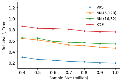
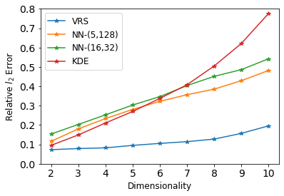
Figure 2: The plot on the left corresponds to Simulation $\mathbf{I}$ with $d=10$ and $N$ varying from $0.4$ million to $1$ million; the plot on the right corresponds to Simulation $\mathbf{I}$ with $N$ being 1 million and $d$ varying from $2$ to $10$.

$\bullet$ Simulation $\mathbf{II}$. Ginzburg-Landau theory is widely used to model microscopic behavior of superconductors. The Ginzburg-Landau density has the following expression,

$$p^{*}(x_{1},\ldots,x_{d})\propto\exp\left(-\beta\sum_{j=0}^{d}\bigg{\{}\frac{\lambda}{2}(\frac{x_{j}-x_{j+1}}{h})^{2}+\frac{1}{4\lambda}(x_{j}^{2}-\frac{1}{16})^{2}\bigg{\}}\right)$$

where $x_{0}=x_{d+1}=0$ and $(x_{1},\ldots,x_{d})\in[-1,1]^{d}$. We sample data from the Ginzburg-Landau density with coefficient $\beta=4,\lambda=1/16,h=1/4$ using Metropolis-Hastings sampling algorithm. We consider two sets of experiments for the Ginzburg-Landau density model. In the first set of experiments, we fix $d=10$ and change the sample size $N$ from $0.4$ million to $1$ million. In the second set of experiments, we keep the sample size $N$ at $1$ million and vary $d$ from $2$ to $10$. We summarize the averaged relative ${{\bf L}_{2}}$-error for each method in Figure 3.

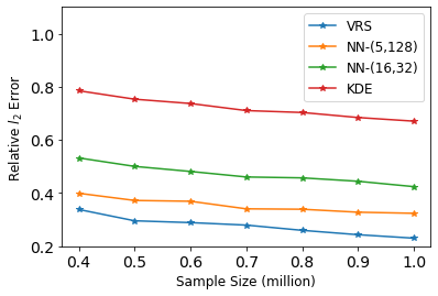
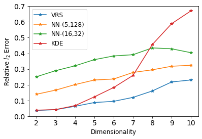
Figure 3: The plot on the left corresponds to Simulation $\mathbf{II}$ with $d=10$ and $N$ varying from $0.4$ million to $1$ million; the plot on the right corresponds to Simulation $\mathbf{II}$ with $N$ being 1 million and $d$ varying from $2$ to $10$.

$\bullet$ Real data $\mathbf{I}$. We analyze the density estimation for the Portugal wine quality dataset from UCI Machine Learning Repository. This dataset contains $6497$ samples of red and white wines, along with $8$ continuous variables: volatile acidity, citric acid, residual sugar, chlorides, free sulfur dioxide, density, sulphates, and alcohol. To provide a comprehensive comparison between different methods, we estimate the joint density of the first $d$ variables in this dataset, allowing $d$ to vary from 2 to 8. For instance, $d=2$ corresponds to the joint density of volatile acidity and citric acid. Since the true density is unknown, we randomly split the dataset into 90% training and 10% test data and evaluate the performance of various approaches using the averaged log-likelihood of the test data. The averaged log-likelihood is defined as follows: let $\widetilde{p}$ be the density estimator based on the training data. The averaged log-likelihood of the test data $\{Z_{i}\}_{i=1}^{N_{\text{test}}}$ is

$$\frac{1}{N_{\text{test}}}\sum_{i=1}^{N_{\text{test}}}\log\{\widetilde{p}(Z_{i})\}.$$

The numerical performance of VRS, NN, and KDE are summarized in Figure 4. Notably, VRS achieves the highest averaged log-likelihood values, indicating its superior numerical performance.

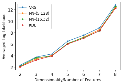
Figure 4: Density estimation for the Portugal wine quality dataset with VRS, KDE, and neural network estimators.

5.3 Nonparametric regression

We analyze the numerical performance of VRS, Nadaraya–Watson kernel regression (NWKR) estimators, and neural networks (NN) in various nonparametric regression problems. The implementation of VRS is provided in Algorithm 3 and the inputs of VRS in the regression setting are detailed in Corollary 3. For neural network estimators, we use the feedforward architecture that are either wide and deep. We measure the estimation accuracy by relative ${{\bf L}_{2}}$-error defined as

$$\frac{\|f^{*}-\widetilde{f}\|_{{{\bf L}_{2}}(\Omega)}}{\|f^{*}\|_{{{\bf L}_{2}}(\Omega)}},$$

where $\widetilde{f}$ is the regression function estimator of a given method. The subsequent simulations and real data examples consistently demonstrate that VRS outperforms both NN and NWKR in a range of nonparametric regression problems.

$\bullet$ Simulation $\mathbf{III}$. We sample data $\{W_{i},Z_{i}\}_{i=1}^{N}\subset\mathbb{R}\times[-1,1]^{d}$ from the regression model

$$W_{i}=f^{*}(Z_{i})+\epsilon_{i},$$

where $\{\epsilon_{i}\}_{i=1}^{N}$ are independently sampled from standard normal distribution, $\{Z_{i}\}_{i=1}^{N}$ are sampled from the uniform distribution on $[-1,1]^{d}$, and

$$f^{*}(x_{1},\ldots,x_{d})=\sin\big{(}\sum_{j=1}^{d}x_{j}\big{)}\quad\text{for }(x_{1},\ldots,x_{d})\in[-1,1]^{d}.$$

In the first set of experiments, we set $d=5$ and vary sample size $N$ from $0.1$ million to $1$ million. In the second set of experiments, the sample size $N$ is fixed at $1$ million, while the dimensionality $d$ varies from $2$ to $10$. Each experimental setup is replicated 100 times to ensure robustness, and we present the average relative $l_{2}$-error for each method in Figure 5.

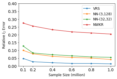
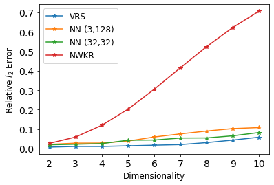
Figure 5: The plot on the left corresponds to Simulation $\mathbf{III}$ with $d=5$ and $N$ varying from $0.1$ million to $1$ million; the plot on the right corresponds to Simulation $\mathbf{III}$ with $N$ being 1 million and $d$ varying from $2$ to $10$.

$\bullet$ Simulation $\mathbf{IV}$. We sample data $\{W_{i},Z_{i}\}_{i=1}^{N}\subset\mathbb{R}\times[-1,1]^{d}$ from the regression model

$$W_{i}=f^{*}(Z_{i})+\epsilon_{i},$$

where $\{\epsilon_{i}\}_{i=1}^{N}$ are independently sampled from standard normal distribution, and $\{Z_{i}\}_{i=1}^{N}$ are independently sampled in $[-1,1]^{d}$ from a $d$-dimensional truncated Gaussian distribution with mean vector $0$ and covariance matrix $4I_{d}$. Here $I_{d}$ is the identity matrix in $d$-dimensions. In addition,

$$f^{*}(x_{1},\ldots,x_{d})=\frac{1}{2}\exp\left(-\frac{1}{d}\sum_{i=1}^{d}\frac{3x_{i}^{2}+1}{4}\right)+\frac{1}{2}\exp\left(-\frac{1}{d}\sum_{i=1}^{d}\frac{7x_{i}^{2}+1}{8}\right)$$

for $(x_{1},\ldots,x_{d})\in[-1,1]^{d}$. In the first set of experiments, we fix $d=5$ and vary $N$ vary from $0.1$ million to $1$ million. In the second set of experiments, we fix the sample size $N$ at $1$ million and let $d$ vary from $2$ to $10$. We repeat each experiment setting $100$ times and report the averaged relative ${{\bf L}_{2}}$-error for each method in Figure 6.

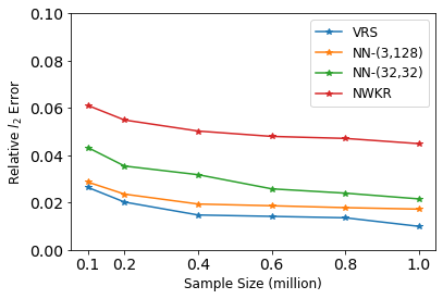
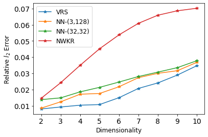
Figure 6: The plot on the left corresponds to Simulation $\mathbf{IV}$ with $d=5$ and $N$ varying from $0.1$ million to $1$ million; the plot on the right corresponds to Simulation $\mathbf{IV}$ with $N$ being 1 million and $d$ varying from $2$ to $10$.

$\bullet$ Real data $\mathbf{II}$. We study the problem of predicting the house price in California using the California housing dataset. This dataset contains $20640$ house price data from the 1990 California census, along with $8$ continuous features such as locations, median house age, and total number bedrooms for house price prediction. Since the true regression function is unknown, we randomly split the dataset into 90% training and 10% test data and evaluate the performance of various approaches by relative test error. Let $\widetilde{f}$ be any regression estimator computed based on the training data. The relative test error of this estimator is defined as

$$\sqrt{\frac{1}{N_{\text{test}}}\sum_{i=1}^{N_{\text{test}}}\frac{(\widetilde{f}(Z_{i})-W_{i})^{2}}{W_{i}^{2}}},$$

where $\{Z_{i},W_{i}\}_{i=1}^{N_{\text{test}}}$ are the test data. The relative test errors for VRS, NWKR, and NN are $0.0275$, $0.0367$, and $0.0285$, respectively, showing that VRS numerical surpasses other methods in this real data example.

5.4 PCA in the continuum-limit

Principal Component Analysis (PCA) in the continuum-limit is a popular technique for reducing noise in images. In this subsection, we examine the numerical performance of VRS in image denoising problems. The state-of-the-art method in image denoising literature is kernel PCA. We direct interested readers to Mika et al. (1998) and Bakır et al. (2004) for a comprehensive introduction to the kernel PCA method.

The main advantage of VRS lies in its computational complexity. Consider $N$ image data with resolution ${\kappa}^{2}$, where $N,{\kappa}\in\mathbb{N}$. The time complexity of kernel PCA is $\operatorname*{O}(N^{2}{\kappa}^{2}+N^{3})$, where $\operatorname*{O}(N^{2}{\kappa}^{2})$ corresponds to the cost of generating the kernel matrix in $\mathbb{R}^{N\times N}$, and $\operatorname*{O}(N^{3})$ reflects the cost of computing the principal components of this matrix. In contrast, the time complexity of VRS is analyzed in (36) with $d=2$. Empirical evidence (see e.g., Pope et al. (2021)) suggests that image data possesses low intrinsic dimensions, making practical choices of $\ell_{j}$ and $r_{j}$ in (36) significantly smaller than $N$ and ${\kappa}$. Even in the worst case scenario where $M$ takes the upper bound ${\kappa}$ in (36), the practical time complexity of VRS is $\operatorname*{O}(N{\kappa}^{2}+{\kappa}^{4})$ which is considerably more efficient than the kernel PCA approach.

In the numerical experiments, we work with real datasets and we treat images from these real datasets as the ground truth images. To evaluate the numerical performance of a given approach, we add i.i.d. Gaussian noise to each pixels of the images and randomly split the dataset into 90% training and 10% test data. We then use the training data to compute the principal components based on the given approach and project the test data onto these estimated principal components. Denote the noiseless ground truth image as $\{{\mathnormal{I}}^{*}_{i}\}_{i=1}^{N_{\text{test}}}$, the corresponding projected noisy test data as $\{\widetilde{{\mathnormal{I}}}_{i}\}_{i=1}^{N_{\text{test}}}$ and the corresponding Gaussian noise added in the images as $\{\epsilon_{i}\}_{i=1}^{N_{\text{test}}}$ in (50). The numerical performance of the given approach is evaluated through the relative denoising error:

$$\sqrt{\frac{1}{N_{\text{test}}}\sum_{i=1}^{N_{\text{test}}}\frac{\|\widetilde{{\mathnormal{I}}}_{i}-{\mathnormal{I}}^{*}_{i}\|^{2}_{2}}{\|{\mathnormal{I}}^{*}_{i}\|^{2}_{2}}}$$

where $\|{{\mathnormal{I}}}^{*}_{i}\|_{2}$ indicates the euclidean norm of ${{\mathnormal{I}}}^{*}_{i}$. We use the relative variance $\sqrt{\frac{1}{N_{\text{test}}}\sum_{i=1}^{N_{\text{test}}}\|\epsilon_{i}\|^{2}_{2}/\|{\mathnormal{I}}^{*}_{i}\|^{2}_{2}}$ to measure the noise level. For the time complexity comparison, we execute on Google Colab’s CPU with high RAM and the execution time of each method is recorded.

$\bullet$ Real data $\mathbf{III}$. Our first study focuses the USPS digits dataset. This dataset comprises images of handwritten digits (0 through 9) that were originally scanned from envelopes by the USPS. It contains a total of 9,298 images, each with a resolution of $16\times 16$. After adding the Gaussian noise, the relative noise variance of the noisy data is 0.7191. The relative denoising errors for VRS and kernel PCA are 0.2951 and 0.2959, respectively, which reflects excellent denoising performance of both two methods. Although the error shows minimal difference, the computational cost of VRS is significantly lower than that of kernel PCA: the execution time for VRS is 0.40 seconds, compared to 36.91 seconds for kernel PCA. In addition to this numerical comparison, in Figure 7(a) we have randomly selected five images from the test set to illustrate the denoised results using VRS and kernel PCA.

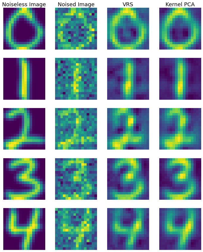
a USPS digits dataset

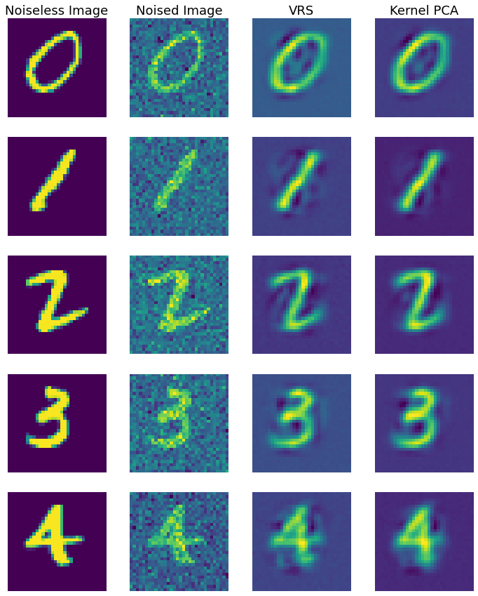
b MNIST dataset

Figure 7: Denoising images from (a) USPS digits dataset and (b) MNIST dataset. In both (a) and (b), the first column shows the ground truth images from the test data, the second column shows the images polluted by Gaussian noise, the third column shows the images denoised using VRS, and the last column shows the images denoised using kernel PCA. Additional numerical results are shown in Appendix H.

$\bullet$ Real data $\mathbf{IV}$. We analyze the MNIST dataset, which comprises 70,000 images of handwritten digits (0 through 9), each labeled with the true digit. The size of each image is $28\times 28$. After adding the Gaussian noise, the relative noise variance of the noisy data is 0.9171. The relative denoising errors for VRS and kernel PCA are 0.4044 and 0.4170, respectively. Although the numerical accuracy of the two methods is quite similar, the computational cost of VRS is significantly lower than that of kernel PCA. The execution time for VRS is only 4.33 seconds, in contrast to 3218.35 seconds for kernel PCA. In addition to this numerical comparison, Figure 7 includes a random selection of five images from the test set to demonstrate the denoised images using VRS and kernel PCA.

6 Conclusion

In this paper, we develop a comprehensive framework Variance-Reduced Sketching (VRS) for nonparametric problems in higher dimensions. Our approach leverages the concept of sketching from numerical linear algebra to address the curse of dimensionality in function spaces. Our method treats multivariable functions as infinite-dimensional matrices or tensors and the selection of sketching is specifically tailored to the regularity of the estimated function. This design takes the variance of random samples in nonparametric problems into consideration, intended to reduce curse of dimensionality in estimation problems. Extensive simulated experiments and real data examples demonstrate that our sketching-based method substantially outperforms both neural network estimators and classical kernel methods in terms of numerical performance.

Appendix A Examples of $\mathcal{M}$ and $\mathcal{L}$ satisfying 2

In this section, we provide three examples of the subspaces $\mathcal{M}$ and $\mathcal{L}$ such that 2 holds.

A.1 Reproducing kernel Hilbert space basis

Let $\mathcal{O}$ be a measurable set in $\mathbb{R}$. The two most used examples are $\mathcal{O}=[0,1]$ for non-parametric estimation and $\mathcal{O}=\{1,\ldots,{\kappa}\}$ for image PCA.

For $x,y\in\mathcal{O}$, let $\mathbb{K}:\mathcal{O}\times\mathcal{O}\to\mathbb{R}$ be a kernel function such that

$$\mathbb{K}(x,y)=\sum_{k=1}^{\infty}\lambda^{\mathbb{K}}_{k}\phi^{\mathbb{K}}_{k}(x)\phi^{\mathbb{K}}_{k}(y),$$ (55)

where $\{\lambda^{\mathbb{K}}_{k}\}_{k=1}^{\infty}\subset\mathbb{R}^{+}\cup\{0\}$ , and $\{\phi^{\mathbb{K}}_{k}\}_{k=1}^{\infty}$ is a collection of basis functions in ${{\bf L}_{2}}(\mathcal{O})$. If $\mathcal{O}=[0,1]$, $\{\phi^{\mathbb{K}}_{k}\}_{k=1}^{\infty}$ are orthonormal ${{\bf L}_{2}}([0,1])$ functions. If $\mathcal{O}=\{1,\ldots,{\kappa}\}$, then $\{\phi^{\mathbb{K}}_{k}\}_{k=1}^{\infty}$ can be identified as orthogonal vectors in $\mathbb{R}^{{\kappa}}$. In this case, $\lambda^{\mathbb{K}}_{k}=0$ for all $k>{\kappa}$.

The reproducing kernel Hilbert space generated by $\mathbb{K}$ is

$${\mathcal{H}}(\mathbb{K})=\bigg{\{}f\in{{\bf L}_{2}}([0,1]):\|f\|_{{\mathcal{H}}(\mathbb{K})}^{2}=\sum_{k=1}^{\infty}(\lambda_{k}^{\mathbb{K}})^{-1}\langle f,\phi^{\mathbb{K}}_{k}\rangle^{2}<\infty\bigg{\}}.$$ (56)

For any functions $f,g\in{\mathcal{H}}(\mathbb{K})$, the inner product in ${\mathcal{H}}(\mathbb{K})$ is given by

$$\langle f,g\rangle_{{\mathcal{H}}(\mathbb{K})}=\sum_{k=1}^{\infty}(\lambda_{k}^{\mathbb{K}})^{-1}\langle f,\phi^{\mathbb{K}}_{k}\rangle\langle g,\phi^{\mathbb{K}}_{k}\rangle.$$

Denote $\Theta^{\mathbb{K}}_{k}=(\lambda^{\mathbb{K}}_{k})^{-1/2}\phi^{\mathbb{K}}_{k}.$ Then $\{\Theta^{\mathbb{K}}_{k}\}_{k=1}^{\infty}$ are the orthonormal basis functions in ${\mathcal{H}}(\mathbb{K})$ as we have that

$$\langle\Theta_{k_{1}}^{\mathbb{K}},\Theta_{k_{2}}^{\mathbb{K}}\rangle_{{\mathcal{H}}(\mathbb{K})}=\begin{cases}1,&\text{if }{k_{1}}={k_{2}};\\ 0,&\text{if }{k_{1}}\not={k_{2}}.\end{cases}$$

an that

$$\|f\|_{{\mathcal{H}}(\mathbb{K})}^{2}=\sum_{k=1}^{\infty}(\lambda_{k}^{\mathbb{K}})^{-1}\langle f,\phi^{\mathbb{K}}_{k}\rangle^{2}=\sum_{k=1}^{\infty}\langle f,\Theta_{k}^{\mathbb{K}}\rangle^{2}.$$

Define the tensor product space

$$\underbrace{{\mathcal{H}}(\mathbb{K}))\otimes\cdots\otimes{\mathcal{H}}(\mathbb{K})}_{d\text{ copies}}=\{{\mathcal{H}}(\mathbb{K})\}^{\otimes d}.$$

The induced Frobenius norm in $\{{\mathcal{H}}(\mathbb{K})\}^{\otimes d}$ is

$$\|A\|_{\{{\mathcal{H}}(\mathbb{K})\}^{\otimes d}}^{2}=\sum_{k_{1},\ldots,k_{d}=1}^{\infty}\big{(}A[\Theta^{\mathbb{K}}_{k_{1}},\ldots,\Theta_{k_{d}}^{\mathbb{K}}]\big{)}^{2}=\sum_{k_{1},\ldots,k_{d}=1}^{\infty}(\lambda_{k_{1}}^{\mathbb{K}}\ldots\lambda_{k_{d}}^{\mathbb{K}})^{-1}\big{(}A[\phi^{\mathbb{K}}_{k_{1}},\ldots,\phi^{\mathbb{K}}_{k_{d}}]\big{)}^{2},$$ (57)

where $A[\phi^{\mathbb{K}}_{k_{1}},\ldots,\phi_{k_{d}}^{\mathbb{K}}]$ is defined by (4). The following lemma shows that the space $\{{\mathcal{H}}(\mathbb{K})\}^{\otimes d}$ is naturally motivated by multidimensional Sobolev spaces.

Lemma 1.

Let $\mathcal{O}=[0,1]$. With $\lambda^{\mathbb{K}}_{k}\asymp k^{-2\alpha}$ and suitable choices of $\{\phi^{\mathbb{K}}_{k}\}_{k=1}^{\infty}$, it holds that

$$\{\mathcal{H}(\mathbb{K})\}^{\otimes d}=W^{\alpha}_{2}([0,1]^{d}).$$

Proof.

Let $\mathcal{O}=[0,1]$. When $d=1$, it is a classical Sobolev space result that with $\lambda^{\mathbb{K}}_{k}\asymp k^{-2\alpha}$ and suitable choices of $\{\phi^{\mathbb{K}}_{k}\}_{k=1}^{\infty}$,

$$\mathcal{H}(\mathbb{K})=W^{\alpha}_{2}([0,1]).$$

We refer interested readers to Chapter 12 of Wainwright (2019) for more details. In general, it is well-known in functional analysis that for $\Omega_{1}\subset\mathbb{R}^{d_{1}}$ and $\Omega_{2}\subset\mathbb{R}^{d_{2}}$, then

$$W^{\alpha}_{2}(\Omega_{1})\otimes W^{\alpha}_{2}(\Omega_{2})=W^{\alpha}_{2}(\Omega_{1}\times\Omega_{2}).$$

Therefore by induction

$$\{\mathcal{H}(\mathbb{K})\}^{\otimes d}=\{\mathcal{H}(\mathbb{K})\}^{\otimes d-1}\otimes\{\mathcal{H}(\mathbb{K})\}=W^{\alpha}_{2}([0,1]^{d-1})\otimes W^{\alpha}_{2}([0,1])=W^{\alpha}_{2}([0,1]^{d}).$$ (58)

∎

Let $(z_{1},\ldots,z_{d_{1}},z_{d_{1}+1},\ldots,z_{d})\in\mathcal{O}^{d}.$ In what follows, we show 2 holds when

$$\mathcal{M}=\text{span}\bigg{\{}\phi^{\mathbb{K}}_{{\mu}_{1}}(z_{1})\cdots\phi^{\mathbb{K}}_{{\mu}_{d_{1}}}(z_{d_{1}})\bigg{\}}_{{\mu}_{1},\ldots,{\mu}_{d_{1}}=1}^{m}\quad\text{and}\quad\mathcal{L}=\text{span}\bigg{\{}\phi^{\mathbb{K}}_{{\eta}_{1}}(z_{d_{1}+1})\cdots\phi^{\mathbb{K}}_{{\eta}_{d_{2}}}(z_{d})\bigg{\}}_{{\eta}_{1},\ldots,{\eta}_{d_{2}}=1}^{\ell}.$$

Lemma 2.

Let $\mathbb{K}$ be a kernel in the form of (55). Suppose that $\lambda^{\mathbb{K}}_{k}\asymp k^{-2\alpha}$, and that $A:\mathcal{O}^{d}\to\mathbb{R}$ is such that $\|A\|_{\{{\mathcal{H}}(\mathbb{K})\}^{\otimes d}}<\infty$. Then for any two positive integers $m,\ell\in\mathbb{Z}^{+}$, it holds that

$$\|A-A\times_{x}\mathcal{P}_{\mathcal{M}}\times_{y}\mathcal{P}_{\mathcal{L}}\|^{2}_{{{\bf L}_{2}}(\mathcal{O}^{d})}\leq C(d_{1}m^{-2\alpha}+d_{2}\ell^{-2\alpha})\|A\|_{\{{\mathcal{H}}(\mathbb{K})\}^{\otimes d}}^{2},$$ (59)

where $C$ is some absolute constant. Consequently

$$\|A-A\times_{y}\mathcal{P}_{\mathcal{L}}\|^{2}_{{{\bf L}_{2}}(\mathcal{O}^{d})}\leq Cd_{2}\ell^{-2\alpha}\|A\|_{\{{\mathcal{H}}(\mathbb{K})\}^{\otimes d}}^{2}\quad\text{and}$$ (60)

$$\|A\times_{y}\mathcal{P}_{\mathcal{L}}-A\times_{x}\mathcal{P}_{\mathcal{M}}\times_{y}\mathcal{P}_{\mathcal{L}}\|^{2}_{{{\bf L}_{2}}(\mathcal{O}^{d})}\leq Cd_{1}m^{-2\alpha}\|A\|_{\{{\mathcal{H}}(\mathbb{K})\}^{\otimes d}}^{2}.$$ (61)

Proof.

Since $\lambda^{\mathbb{K}}_{k}\asymp k^{-2\alpha}$, without loss of generality, throughout the proof we assume that

$$\lambda^{\mathbb{K}}_{k}=k^{-2\alpha},$$

as otherwise all of our analysis still holds up to an absolute constant. Observe that

$$\left(A\times_{x}\mathcal{P}_{\mathcal{M}}\times_{y}\mathcal{P}_{\mathcal{L}}\right)[\phi^{\mathbb{K}}_{{\mu}_{1}},\ldots,\phi^{\mathbb{K}}_{{\mu}_{d_{1}}},\phi^{\mathbb{K}}_{{\eta}_{1}},\ldots,\phi^{\mathbb{K}}_{{\eta}_{d_{2}}}]$$

$$= \begin{cases}A[\phi^{\mathbb{K}}_{{\mu}_{1}},\ldots,\phi^{\mathbb{K}}_{{\mu}_{d_{1}}},\phi^{\mathbb{K}}_{{\eta}_{1}},\ldots,\phi^{\mathbb{K}}_{{\eta}_{d_{2}}}],&\text{if }1\leq{\mu}_{1},\ldots,{\mu}_{d_{1}}\leq m$ and $1\leq{\eta}_{1},\ldots,{\eta}_{d_{2}}\leq\ell,\\ 0,&\text{otherwise.}\end{cases}$$

Then

$$\|A-A\times_{x}\mathcal{P}_{\mathcal{M}}\times_{y}\mathcal{P}_{\mathcal{L}}\|^{2}_{{{\bf L}_{2}}(\mathcal{O}^{d})}= \sum_{{\mu}_{1}=m+1}^{\infty}\sum_{{\mu}_{2},\ldots,{\mu}_{d_{1}}=1}^{m}\sum_{{\eta}_{1},\ldots,{\eta}_{d_{2}}=1}^{\ell}\big{(}A[\phi^{\mathbb{K}}_{{\mu}_{1}},\ldots,\phi^{\mathbb{K}}_{{\mu}_{d_{1}}},\phi^{\mathbb{K}}_{{\eta}_{1}},\ldots,\phi^{\mathbb{K}}_{{\eta}_{d_{2}}}]\big{)}^{2}$$

$$+ \ldots$$

$$+ \sum_{{\mu}_{1},\ldots,{\mu}_{d_{1}}=1}^{m}\sum_{{\eta}_{1},\ldots,{\eta}_{d_{2}-1}=1}^{\ell}\sum_{{\eta}_{d_{2}}=\ell+1}^{\infty}\big{(}A[\phi^{\mathbb{K}}_{{\mu}_{1}},\ldots,\phi^{\mathbb{K}}_{{\mu}_{d_{1}}},\phi^{\mathbb{K}}_{{\eta}_{1}},\ldots,\phi^{\mathbb{K}}_{{\eta}_{d_{2}}}]\big{)}^{2}.$$

Observe that

$$\sum_{{\mu}_{1}=m+1}^{\infty}\sum_{{\mu}_{2},\ldots,{\mu}_{d_{1}}=1}^{m}\sum_{{\eta}_{1},\ldots,{\eta}_{d_{2}}=1}^{\ell}\big{(}A[\phi^{\mathbb{K}}_{{\mu}_{1}},\ldots,\phi^{\mathbb{K}}_{{\mu}_{d_{1}}},\phi^{\mathbb{K}}_{{\eta}_{1}},\ldots,\phi^{\mathbb{K}}_{{\eta}_{d_{2}}}]\big{)}^{2}$$

$$\leq \sum_{{\mu}_{1}=m+1}^{\infty}m^{-2\alpha}{\mu}_{1}^{2\alpha}\sum_{{\mu}_{2},\ldots,{\mu}_{d_{1}}=1}^{m}\sum_{{\eta}_{1},\ldots,{\eta}_{d_{2}}=1}^{\ell}\big{(}A[\phi^{\mathbb{K}}_{{\mu}_{1}},\ldots,\phi^{\mathbb{K}}_{{\mu}_{d_{1}}},\phi^{\mathbb{K}}_{{\eta}_{1}},\ldots,\phi^{\mathbb{K}}_{{\eta}_{d_{2}}}]\big{)}^{2}$$

$$\leq m^{-2\alpha}\sum_{{\mu}_{1}=m+1}^{\infty}\sum_{{\mu}_{2},\ldots,{\mu}_{d_{1}}=1}^{m}\sum_{{\eta}_{1},\ldots,{\eta}_{d_{2}}=1}^{\ell}{\mu}_{1}^{2\alpha}\cdots{\mu}_{d_{1}}^{2\alpha}{\eta}_{1}^{2\alpha}\cdots{\eta}_{d_{2}}^{2\alpha}\big{(}A[\phi^{\mathbb{K}}_{{\mu}_{1}},\ldots,\phi^{\mathbb{K}}_{{\mu}_{d_{1}}},\phi^{\mathbb{K}}_{{\eta}_{1}},\ldots,\phi^{\mathbb{K}}_{{\eta}_{d_{2}}}]\big{)}^{2}$$

$$\leq m^{-2\alpha}\sum_{{\mu}_{1}=1}^{\infty}\sum_{{\mu}_{2},\ldots,{\mu}_{d_{1}}=1}^{\infty}\sum_{{\eta}_{1},\ldots,{\eta}_{d_{2}}=1}^{\infty}{\mu}_{1}^{2\alpha}\cdots{\mu}_{d_{1}}^{2\alpha}{\eta}_{1}^{2\alpha}\cdots{\eta}_{d_{2}}^{2\alpha}\big{(}A[\phi^{\mathbb{K}}_{{\mu}_{1}},\ldots,\phi^{\mathbb{K}}_{{\mu}_{d_{1}}},\phi^{\mathbb{K}}_{{\eta}_{1}},\ldots,\phi^{\mathbb{K}}_{{\eta}_{d_{2}}}]\big{)}^{2}$$

$$= m^{-2\alpha}\|A\|_{\{{\mathcal{H}}(\mathbb{K})\}^{\otimes d}}^{2}$$

where the first inequality holds because ${\mu}_{1}\geq m+1\geq m$ and the last equality follows from (57). Similarly

$$\sum_{{\mu}_{1},\ldots,{\mu}_{d_{1}}=1}^{m}\sum_{{\eta}_{1},\ldots,{\eta}_{d_{2}-1}=1}^{\ell}\sum_{{\eta}_{d_{2}}=\ell+1}^{\infty}\big{(}A[\phi^{\mathbb{K}}_{{\mu}_{1}},\ldots,\phi^{\mathbb{K}}_{{\mu}_{d_{1}}},\phi^{\mathbb{K}}_{{\eta}_{1}},\ldots,\phi^{\mathbb{K}}_{{\eta}_{d_{2}}}]\big{)}^{2}$$

$$\leq \sum_{{\mu}_{1},\ldots,{\mu}_{d_{1}}=1}^{m}\sum_{{\eta}_{1},\ldots,{\eta}_{d_{2}-1}=1}^{\ell}\sum_{{\eta}_{d_{2}}=\ell+1}^{\infty}\ell^{-2\alpha}{\eta}_{d_{2}}^{2\alpha}\big{(}A[\phi^{\mathbb{K}}_{{\mu}_{1}},\ldots,\phi^{\mathbb{K}}_{{\mu}_{d_{1}}},\phi^{\mathbb{K}}_{{\eta}_{1}},\ldots,\phi^{\mathbb{K}}_{{\eta}_{d_{2}}}]\big{)}^{2}$$

$$\leq \ell^{-2\alpha}\sum_{{\mu}_{1},\ldots,{\mu}_{d_{1}}=1}^{m}\sum_{{\eta}_{1},\ldots,{\eta}_{d_{2}-1}=1}^{\ell}\sum_{{\eta}_{d_{2}}=\ell+1}^{\infty}{\mu}_{1}^{2\alpha}\cdots{\mu}_{d_{1}}^{2\alpha}{\eta}_{1}^{2\alpha}\cdots{\eta}_{d_{2}}^{2\alpha}\big{(}A[\phi^{\mathbb{K}}_{{\mu}_{1}},\ldots,\phi^{\mathbb{K}}_{{\mu}_{d_{1}}},\phi^{\mathbb{K}}_{{\eta}_{1}},\ldots,\phi^{\mathbb{K}}_{{\eta}_{d_{2}}}]\big{)}^{2}$$

$$\leq \ell^{-2\alpha}\|A\|_{\{{\mathcal{H}}(\mathbb{K})\}^{\otimes d}}^{2},$$

where the first inequality holds because ${\eta}_{d_{2}}\geq\ell+1\geq\ell$ and the last inequality follows from (57). Thus (59) follows immediately.

For (60), note that when $m=\infty$, $\mathcal{M}={{\bf L}_{2}}(\mathcal{O}^{d_{1}})$. In this case $\mathcal{P}_{\mathcal{M}}$ becomes the identity operator and

$$A\times_{x}\mathcal{P}_{\mathcal{M}}\times_{y}\mathcal{P}_{\mathcal{L}}=A\times_{y}\mathcal{P}_{\mathcal{L}}.$$

Therefore (60) follows from (59) by taking $m=\infty$.

For (61), similar to (60), we have that

$$\|A-A\times_{x}\mathcal{P}_{\mathcal{M}}\|^{2}_{{{\bf L}_{2}}(\mathcal{O}^{d})}\leq Cd_{1}m^{-2\alpha}\|A\|_{\{{\mathcal{H}}(\mathbb{K})\}^{\otimes d}}^{2}.$$

It follows that

$$\|A\times_{y}\mathcal{P}_{\mathcal{L}}-A\times_{x}\mathcal{P}_{\mathcal{M}}\times_{y}\mathcal{P}_{\mathcal{L}}\|^{2}_{{{\bf L}_{2}}(\mathcal{O}^{d})}\leq\|A-A\times_{x}\mathcal{P}_{\mathcal{M}}\|^{2}_{{{\bf L}_{2}}(\mathcal{O}^{d})}\|\mathcal{P}_{\mathcal{L}}\|^{2}_{\operatorname*{op}}\leq Cd_{1}m^{-2\alpha}\|A\|_{\{{\mathcal{H}}(\mathbb{K})\}^{\otimes d}}^{2},$$

where last inequality follows from the fact that $\|\mathcal{P}_{\mathcal{L}}\|_{\operatorname*{op}}\leq 1$. ∎

A.2 Legendre polynomial basis

Legendre polynomials is a well-known classical orthonormal polynomial system in ${{\bf L}_{2}}([-1,1])$. We can define the Legendre polynomials in the following inductive way. Let $p_{0}=1$ and suppose $\{p_{k}\}_{k=1}^{n-1}$ are defined. Let $p_{n}:[-1,1]\to\mathbb{R}$ be a polynomial of degree $n$ such that
$\bullet$ $\|p_{n}\|_{{{\bf L}_{2}}([-1,1])}=1$, and
$\bullet$ $\int_{-1}^{1}p_{n}(x)p_{k}(x)\mathrm{d}x=0$ for all $0\leq k\leq n-1$.
As a quick example, we have that

$$p_{0}(x)=1,\quad p_{1}(x)=\sqrt{\frac{3}{2}}x,\quad\text{and}\quad p_{2}(x)=\sqrt{\frac{5}{3}}\frac{3x^{2}-1}{2}.$$

Let $q_{k}(x)=\sqrt{2}p_{k}(2x-1)$. Then $\{q_{k}\}_{k=0}^{\infty}$ are the orthonormal polynomial system in ${{\bf L}_{2}}([0,1])$. In this subsection, we show that 2 holds when $\{\phi^{\mathbb{S}}_{k}\}_{k=1}^{\infty}$ in (5) is chosen to be $\{q_{k}\}_{k=0}^{\infty}$. More precisely, let

$$\mathbb{S}_{n}=\operatorname*{Span}\{q_{k}\}_{k=0}^{n}$$

and $\mathcal{P}_{\mathbb{S}_{n}}$ denote the projection operator from ${{\bf L}_{2}}([0,1])$ to $\mathbb{S}_{n}$. Then $\mathbb{S}_{n}$ is the subspace of polynomials of degree at most $n$. In addition, for any $f\in{{\bf L}_{2}}([0,1])$, $\mathcal{P}_{\mathbb{S}_{n}}(f)$ is the best $n$-degree polynomial approximation of $f$ in the sense that

$$\|\mathcal{P}_{\mathbb{S}_{n}(z)}(f)-f\|_{{{\bf L}_{2}}([0,1])}=\min_{g\in\mathbb{S}_{n}}\|g-f\|_{{{\bf L}_{2}}([0,1])}.$$ (62)

We begin with a well-known polynomial approximation result. For $\alpha\in\mathbb{Z}^{+}$, denote $C^{\alpha}([0,1])$ to be the class of functions that are $\alpha$ times continuously differentiable.

Theorem 5.

Suppose $f\in C^{\alpha}([0,1])$. Then for any $n\in\mathbb{Z}^{+}$, there exists a polynomial $p_{2n}(f)$ of degree $2n$ such that

$$\|f-p_{2n}(f)\|_{{{\bf L}_{2}}([0,1])}^{2}\leq Cn^{-2\alpha}\|f^{(\alpha)}\|_{{{\bf L}_{2}}([0,1])}^{2},$$

where $C$ is an absolute constant.

Proof.

This is Theorem 1.2 of Xu (2018). ∎

Therefore by (62) and Theorem 5,

$$\|\mathcal{P}_{\mathbb{S}_{n}(z)}(f)-f\|^{2}_{{{\bf L}_{2}}([0,1])}\leq\|f-p_{\lfloor n/2\rfloor}(f)\|_{{{\bf L}_{2}}([0,1])}^{2}\leq C^{\prime}n^{-2\alpha}\|f^{(\alpha)}\|_{{{\bf L}_{2}}([0,1])}^{2}.$$ (63)

Let $z=(z_{1},\ldots,z_{d})\in\mathbb{R}^{d}$ and let $\mathbb{S}_{n}(z_{j})$ denote the linear space spanned by polynomials of $z_{j}$ of degree at most $n$.

Corollary 5.

Suppose $B(z_{1},\ldots,z_{d})\in C^{\alpha}([0,1]^{d})$. Then for any $1\leq p\leq d$,

$$\|B-B\times_{p}\mathcal{P}_{\mathbb{S}_{n}(z_{p})}\|_{{{\bf L}_{2}}([0,1]^{d})}\leq Cn^{-\alpha}\|B\|_{W^{\alpha}_{2}([0,1]^{d})}.$$

Proof.

It suffices to consider $p=1$. For any fixed $(z_{2},\ldots,z_{d})$, $B(\cdot,z_{2},\ldots,z_{d})\in C^{\alpha}([0,1])$. Therefore by (63),

$$\int\bigg{\{}B(z_{1},z_{2},\ldots,z_{d})-\mathcal{P}_{\mathbb{S}_{n}(z_{1})}(B(z_{1},z_{2},\ldots,z_{d}))\bigg{\}}^{2}\mathrm{d}z_{1}\leq Cn^{-2\alpha}\int\bigg{\{}\frac{\partial^{\alpha}}{\partial^{\alpha}z_{1}}B(z_{1},z_{2},\ldots,z_{d})\bigg{\}}^{2}\mathrm{d}z_{1}.$$

Therefore

$$\int\cdots\int\bigg{\{}B(z_{1},z_{2},\ldots,z_{d})-\mathcal{P}_{\mathbb{S}_{n}(z_{1})}(B(z_{1},z_{2},\ldots,z_{d}))\bigg{\}}^{2}\mathrm{d}z_{1}\mathrm{d}z_{2}\cdots\mathrm{d}z_{d}$$

$$\leq \int\cdots\int Cn^{-2\alpha}\int\bigg{\{}\frac{\partial^{\alpha}}{\partial^{\alpha}z_{1}}B(z_{1},z_{2},\ldots,z_{d})\bigg{\}}^{2}\mathrm{d}z_{1}\mathrm{d}z_{2}\cdots\mathrm{d}z_{d}.$$

The desired result follows from the observation that

$$\mathcal{P}_{\mathbb{S}_{n}(z_{1})}(B(z_{1},z_{2},\ldots,z_{d}))=\big{(}B\times_{1}\mathcal{P}_{\mathbb{S}_{n}(z_{1})}\big{)}(z_{1},z_{2},\ldots,z_{d})$$

and that $\int\cdots\int\big{\{}\frac{\partial^{\alpha}}{\partial^{\alpha}z_{1}}B(z_{1},z_{2},\ldots,z_{d})\big{\}}^{2}\mathrm{d}z_{1}\cdots\mathrm{d}z_{d}\leq\|B\|^{2}_{W^{\alpha}_{2}([0,1]^{d})}$. ∎

Lemma 3.

Under the same conditions as in Corollary 5, it holds that

$$\mathcal{P}_{\mathbb{S}_{n}(z_{1})}(B(z_{1},z_{2},\ldots,z_{d}))=\big{(}B\times_{1}\mathcal{P}_{\mathbb{S}_{n}(z_{1})}\big{)}(z_{1},z_{2},\ldots,z_{d}).$$ (64)

Proof.

Note that $\mathcal{P}_{\mathbb{S}_{n}(z_{1})}$ is a projection operator. So for any $f,g\in{{\bf L}_{2}}([0,1])$,

$$\int_{0}^{1}\mathcal{P}_{\mathbb{S}_{n}(z_{1})}(f(z_{1}))g(z_{1})\mathrm{d}z_{1}=\langle\mathcal{P}_{\mathbb{S}_{n}(z_{1})}(f),g\rangle=\langle f,\mathcal{P}_{\mathbb{S}_{n}(z_{1})}(g)\rangle=\int_{0}^{1}f(z_{1})\mathcal{P}_{\mathbb{S}_{n}(z_{1})}(g(z_{1}))\mathrm{d}z_{1}$$ (65)

Given $(z_{2},\ldots,z_{d})$, $B(\cdot,z_{2},\ldots,z_{d})\in C^{\alpha}([0,1])$ and therefore $\mathcal{P}_{\mathbb{S}_{n}(z_{1})}(B(z_{1},z_{2},\ldots,z_{d}))$ is well-defined and is a function mapping from $[0,1]^{d}$ to $\mathbb{R}$. To show that (64), it suffices to observe that for any test functions $\{u_{j}(z_{j})\}_{j=1}^{d}\in{{\bf L}_{2}}([0,1])$,

$$\mathcal{P}_{\mathbb{S}_{n}(z_{1})}(B(z_{1},z_{2},\ldots,z_{d}))[u_{1}(z_{1}),\ldots,u_{d}(z_{d})]$$

$$= \int_{0}^{1}\cdots\int_{0}^{1}\mathcal{P}_{\mathbb{S}_{n}(z_{1})}(B(z_{1},z_{2},\ldots,z_{d}))u_{1}(z_{1})\cdots u_{d}(z_{d})\mathrm{d}z_{1}\cdots\mathrm{d}z_{d}$$

$$= \int_{0}^{1}\cdots\int_{0}^{1}\bigg{(}\int_{0}^{1}\mathcal{P}_{\mathbb{S}_{n}(z_{1})}(B(z_{1},z_{2},\ldots,z_{d}))u_{1}(z_{1})\mathrm{d}z_{1}\bigg{)}u_{2}(z_{2})\cdots u_{d}(z_{d})\mathrm{d}z_{2}\cdots\mathrm{d}z_{d}$$

$$= \int_{0}^{1}\cdots\int_{0}^{1}\bigg{(}\int_{0}^{1}B(z_{1},z_{2},\ldots,z_{d})\mathcal{P}_{\mathbb{S}_{n}(z_{1})}(u_{1}(z_{1}))\mathrm{d}z_{1}\bigg{)}u_{2}(z_{2})\cdots u_{d}(z_{d})\mathrm{d}z_{2}\cdots\mathrm{d}z_{d}$$

$$= \big{(}B\times_{1}\mathcal{P}_{\mathbb{S}_{n}(z_{1})}\big{)}[u_{1}(z_{1}),\ldots,u_{d}(z_{d})].$$

∎

In what follows, we present a polynomial approximation theory in multidimensions.

Lemma 4.

For $j\in[1,\ldots,d]$, let $\mathbb{S}_{n_{j}}(z_{j})$ denote the linear space spanned by polynomials of $z_{j}$ of degree $n_{j}$ and let $\mathcal{P}_{\mathbb{S}_{n_{j}}(z_{j})}$ be the corresponding projection operator. Then for any $B\in W^{\alpha}_{2}([0,1]^{d})$, it holds that

$$\|B-B\times_{1}\mathcal{P}_{\mathbb{S}_{n_{1}}(z_{1})}\cdots\times_{d}\mathcal{P}_{\mathbb{S}_{n_{d}}(z_{d})}\|_{{{\bf L}_{2}}([0,1]^{d})}\leq C\sum_{j=1}^{d}n_{j}^{-\alpha}\|B\|_{W^{\alpha}_{2}([0,1]^{d})}.$$ (66)

Proof.

Since $C^{\alpha}([0,1]^{d})$ is dense in $W^{\alpha}_{2}([0,1]^{d})$, it suffices to show (66) for all $f\in C^{\alpha}([0,1]^{d})$. We proceed by induction. The base case

$$\|B-B\times_{1}\mathcal{P}_{\mathbb{S}_{n_{1}}(z_{1})}\|_{{{\bf L}_{2}}([0,1]^{d})}\leq Cn_{1}^{-\alpha}\|B\|_{W^{\alpha}_{2}([0,1]^{d})}$$

is a direct consequence of Corollary 5. Suppose by induction, the following inequality holds for $p$,

$$\|B-B\times_{1}\mathcal{P}_{\mathbb{S}_{n_{1}}(z_{1})}\cdots\times_{p}\mathcal{P}_{\mathbb{S}_{n_{p}}(z_{p})}\|_{{{\bf L}_{2}}([0,1]^{d})}\leq C\sum_{j=1}^{p}n_{j}^{-\alpha}\|B\|_{W^{\alpha}_{2}([0,1]^{d})}.$$ (67)

Then

$$\|B-B\times_{1}\mathcal{P}_{\mathbb{S}_{n_{1}}(z_{1})}\cdots\times_{p}\mathcal{P}_{\mathbb{S}_{n_{p}}(z_{p})}\times_{p+1}\mathcal{P}_{\mathbb{S}_{n_{p+1}}(z_{p+1})}\|_{{{\bf L}_{2}}([0,1]^{d})}$$

$$\leq \|B\times_{1}\mathcal{P}_{\mathbb{S}_{n_{1}}(z_{1})}\cdots\times_{p}\mathcal{P}_{\mathbb{S}_{n_{p}}(z_{p})}\times_{p+1}\mathcal{P}_{\mathbb{S}_{n_{p+1}}(z_{p+1})}-B\times_{1}\mathcal{P}_{\mathbb{S}_{n_{1}}(z_{1})}\cdots\times_{p}\mathcal{P}_{\mathbb{S}_{n_{p}}(z_{p})}\|_{{{\bf L}_{2}}([0,1]^{d})}$$

$$+ \|B-B\times_{1}\mathcal{P}_{\mathbb{S}_{n_{1}}(z_{1})}\cdots\times_{p}\mathcal{P}_{\mathbb{S}_{n_{p}}(z_{p})}\|_{{{\bf L}_{2}}([0,1]^{d})}.$$

The desired result follows from (67) and the observation that $\|\mathcal{P}_{\mathbb{S}_{n_{j}}(z_{j})}\|_{\operatorname*{op}}\leq 1$ for all $j$, and therefore

$$\|B\times_{1}\mathcal{P}_{\mathbb{S}_{n_{1}}(z_{1})}\cdots\times_{p}\mathcal{P}_{\mathbb{S}_{n_{p}}(z_{p})}\times_{p+1}\mathcal{P}_{\mathbb{S}_{n_{p+1}}(z_{p+1})}-B\times_{1}\mathcal{P}_{\mathbb{S}_{n_{1}}(z_{1})}\cdots\times_{p}\mathcal{P}_{\mathbb{S}_{n_{p}}(z_{p})}\|_{{{\bf L}_{2}}([0,1]^{d})}$$

$$\leq \|B\times_{p+1}\mathcal{P}_{\mathbb{S}_{n_{p+1}}(z_{p+1})}-B\|_{{{\bf L}_{2}}([0,1]^{d})}\|\mathcal{P}_{\mathbb{S}_{n_{1}}(z_{1})}\|_{\operatorname*{op}}\cdots\|\mathcal{P}_{\mathbb{S}_{n_{p}}(z_{p})}\|_{\operatorname*{op}}$$

$$\leq Cn^{-\alpha}_{p+1}\|B\|_{W^{\alpha}_{2}([0,1]^{d})},$$

where the last inequality follows from Corollary 5. ∎

Note that Lemma 4 directly implies that 2 holds when

$$\mathcal{M}=\mathbb{S}_{m}(z_{1})\otimes\cdots\otimes\mathbb{S}_{m}(z_{d_{1}})\quad\text{and}\quad\mathcal{L}=\mathbb{S}_{\ell}(z_{d_{1}+1})\otimes\cdots\otimes\mathbb{S}_{\ell}(z_{d}).$$

This is summarized in the following lemma.

Lemma 5.

Suppose $\|A\|_{W^{\alpha}_{2}([0,1]^{d})}<\infty$. Then for $1\leq m\leq\infty$ and $1\leq\ell\leq\infty$,

$$\|A-A\times_{x}\mathcal{P}_{\mathcal{M}}\times_{y}\mathcal{P}_{\mathcal{L}}\|^{2}_{\mathcal{L}_{2}([0,1]^{d})}=\operatorname*{O}(m^{-2\alpha}+\ell^{-2\alpha})$$ (68)

$$\|A-A\times_{y}\mathcal{P}_{\mathcal{L}}\|^{2}_{\mathcal{L}_{2}([0,1]^{d})}=\operatorname*{O}(\ell^{-2\alpha})\quad\text{and}$$ (69)

$$\|A\times_{y}\mathcal{P}_{\mathcal{L}}-A\times_{x}\mathcal{P}_{\mathcal{M}}\times_{y}\mathcal{P}_{\mathcal{L}}\|^{2}_{\mathcal{L}_{2}([0,1]^{d})}=\operatorname*{O}(m^{-2\alpha}).$$ (70)

Proof.

For (68), by Lemma 4,

$$\|A-A\times_{x}\mathcal{P}_{\mathcal{M}}\times_{y}\mathcal{P}_{\mathcal{L}}\|_{\mathcal{L}_{2}([0,1]^{d})}\leq C\big{(}d_{1}(m-\alpha-1)^{-\alpha}+d_{2}(\ell-\alpha-1)^{-\alpha}\big{)}\|A\|_{W^{\alpha}_{2}([0,1]^{d})}$$

$$= \operatorname*{O}(m^{-\alpha}+\ell^{-\alpha}),$$

where the equality follows from the fact that $\alpha$, $d_{1}$ and $d_{2}$ are constants.

For (69), note that when $m=\infty$, $\mathcal{M}={{\bf L}_{2}}([0,1]^{d_{1}})$. In this case $\mathcal{P}_{\mathcal{M}}$ becomes the identity operator and

$$A\times_{x}\mathcal{P}_{\mathcal{M}}\times_{y}\mathcal{P}_{\mathcal{L}}=A\times_{y}\mathcal{P}_{\mathcal{L}}.$$

Therefore (69) follows from (68) by taking $m=\infty$.

For (70), similar to (69), we have that

$$\|A-A\times_{x}\mathcal{P}_{\mathcal{M}}\|^{2}_{{{\bf L}_{2}}([0,1]^{d})}=\operatorname*{O}(m^{-2\alpha}).$$

It follows that

$$\|A\times_{y}\mathcal{P}_{\mathcal{L}}-A\times_{x}\mathcal{P}_{\mathcal{M}}\times_{y}\mathcal{P}_{\mathcal{L}}\|^{2}_{{{\bf L}_{2}}([0,1]^{d})}\\ \leq\|A-A\times_{x}\mathcal{P}_{\mathcal{M}}\|^{2}_{{{\bf L}_{2}}([0,1]^{d})}\|\mathcal{P}_{\mathcal{L}}\|^{2}_{\operatorname*{op}}=\operatorname*{O}(m^{-2\alpha}),$$

where last inequality follows from the fact that $\|\mathcal{P}_{\mathcal{L}}\|_{\operatorname*{op}}\leq 1$. ∎

A.3 Spline basis

Let $\alpha\in\mathbb{Z}^{+}$ be given and $\{\xi_{k}\}_{k=1}^{n}\subset[0,1]$ be a collection of grid points such that

$$\xi_{k}=\frac{k}{n}.$$

Denote $\mathbb{S}_{n,\alpha}(x)$ the subspace in ${{\bf L}_{2}}([0,1])$ spanned by the spline functions being peicewise polynomials defined on $\{\xi_{k}\}_{k=1}^{n}$ of degree $\alpha$. Specifically

$$\mathbb{S}_{n,\alpha}(x)=\{\beta_{0}+\beta_{1}b_{1}(x)+\ldots+\beta_{\alpha+n}b_{\alpha+n}(x):\{\beta_{k}\}_{k=0}^{\alpha+n}\subset\mathbb{R}\},$$

where

$$b_{1}(x)=x^{1},\ \ldots,\ b_{\alpha}(x)=x^{\alpha},\ b_{k+\alpha}(x)=(x-\xi_{k})_{+}^{\alpha}\text{ for }k=1,\ldots,n,$$

and

$$(x-\xi_{k})_{+}^{\alpha}=\begin{cases}(x-\xi_{k})^{\alpha},&\text{if }x\geq\xi_{k};\\ 0,&\text{if }x<\xi_{k}.\end{cases}$$

Let $\{\phi^{n,\alpha}_{k}(x)\}_{k=1}^{n+\alpha+1}$ be the ${{\bf L}_{2}}([0,1])$ sub-basis functions spanning $\mathbb{S}_{n,\alpha}(x)$. In this section, we show that 2 holds when

$$\mathcal{M} =\mathbb{S}_{m-\alpha-1,\alpha}(z_{1})\otimes\cdots\otimes\mathbb{S}_{m-\alpha-1,\alpha}(z_{d_{1}})=\text{span}\bigg{\{}\phi^{m-\alpha-1,\alpha}_{{\mu}_{1}}(z_{1})\cdots\phi^{m-\alpha-1,\alpha}_{{\mu}_{d_{1}}}(z_{d_{1}})\bigg{\}}_{{\mu}_{1},\ldots,{\mu}_{d_{1}}=1}^{m},\quad\text{and}$$

$$\mathcal{L} =\mathbb{S}_{\ell-\alpha-1,\alpha}(z_{d_{1}+1})\otimes\cdots\otimes\mathbb{S}_{\ell-\alpha-1,\alpha}(z_{d})=\text{span}\bigg{\{}\phi^{\ell-\alpha-1,\alpha}_{{\eta}_{1}}(z_{d_{1}+1})\cdots\phi^{\ell-\alpha-1,\alpha}_{{\eta}_{d_{2}}}(z_{d})\bigg{\}}_{{\eta}_{1},\ldots,{\eta}_{d_{2}}=1}^{\ell}.$$

where $m$ and $\ell$ are positive integers such that $m>\alpha+1$ and $\ell>\alpha+1$. We begin with a spline space approximation theorem for multivariate functions.

Lemma 6.

Suppose $\|A\|_{W^{\alpha}_{2}([0,1]^{d})}<\infty$. Suppose in addition $\{n_{j}\}_{j=1}^{d}$ is a collection positive integer strictly greater than $\alpha+1$. Then

$$\|A-A\times_{1}\mathcal{P}_{\mathbb{S}_{n_{1}-\alpha-1,\alpha}}(z_{1})\cdots\times_{d}\mathcal{P}_{\mathbb{S}_{n_{d}-\alpha-1,\alpha}}(z_{d})\|\leq C\sum_{j=1}^{d}(n_{j}-\alpha-1)^{-\alpha}\|A\|_{W^{\alpha}_{2}([0,1]^{d})}$$

Proof.

This is Example 13 on page 26 of Sande et al. (2020). ∎

In the following lemma, we justify 2 when $\mathcal{M}=\mathbb{S}_{m-\alpha-1,\alpha}(z_{1})\otimes\cdots\otimes\mathbb{S}_{m-\alpha-1,\alpha}(z_{d_{1}})$ and $\mathcal{L}=\mathbb{S}_{\ell-\alpha-1,\alpha}(z_{d_{1}+1})\otimes\cdots\otimes\mathbb{S}_{\ell-\alpha-1,\alpha}(z_{d})$.

Lemma 7.

Suppose $\|A\|_{W^{\alpha}_{2}([0,1]^{d})}<\infty$ where $\alpha\in\mathbb{Z}^{+}$ is a fixed constant. Then for $1+\alpha\leq m\leq\infty$ and $1+\alpha\leq\ell\leq\infty$,

$$\|A-A\times_{x}\mathcal{P}_{\mathcal{M}}\times_{y}\mathcal{P}_{\mathcal{L}}\|^{2}_{\mathcal{L}_{2}([0,1]^{d})}=\operatorname*{O}(m^{-2\alpha}+\ell^{-2\alpha})$$ (71)

$$\|A-A\times_{y}\mathcal{P}_{\mathcal{L}}\|^{2}_{\mathcal{L}_{2}([0,1]^{d})}=\operatorname*{O}(\ell^{-2\alpha})\quad\text{and}$$ (72)

$$\|A\times_{y}\mathcal{P}_{\mathcal{L}}-A\times_{x}\mathcal{P}_{\mathcal{M}}\times_{y}\mathcal{P}_{\mathcal{L}}\|^{2}_{\mathcal{L}_{2}([0,1]^{d})}=\operatorname*{O}(m^{-2\alpha}).$$ (73)

Proof.

For (71), by Lemma 6,

$$\|A-A\times_{x}\mathcal{P}_{\mathcal{M}}\times_{y}\mathcal{P}_{\mathcal{L}}\|_{\mathcal{L}_{2}([0,1]^{d})}\leq C\big{(}d_{1}(m-\alpha-1)^{-\alpha}+d_{2}(\ell-\alpha-1)^{-\alpha}\big{)}\|A\|_{W^{\alpha}_{2}([0,1]^{d})}$$

$$= \operatorname*{O}(m^{-\alpha}+\ell^{-\alpha}),$$

where the equality follows from the fact that $\alpha$, $d_{1}$ and $d_{2}$ are constants.

For (72), note that when $m=\infty$, $\mathcal{M}={{\bf L}_{2}}([0,1]^{d_{1}})$. In this case $\mathcal{P}_{\mathcal{M}}$ becomes the identity operator and

$$A\times_{x}\mathcal{P}_{\mathcal{M}}\times_{y}\mathcal{P}_{\mathcal{L}}=A\times_{y}\mathcal{P}_{\mathcal{L}}.$$

Therefore (72) follows from (71) by taking $m=\infty$.

For (73), similar to (72), we have that

$$\|A-A\times_{x}\mathcal{P}_{\mathcal{M}}\|^{2}_{{{\bf L}_{2}}([0,1]^{d})}=\operatorname*{O}(m^{-2\alpha}).$$

It follows that

$$\|A\times_{y}\mathcal{P}_{\mathcal{L}}-A\times_{x}\mathcal{P}_{\mathcal{M}}\times_{y}\mathcal{P}_{\mathcal{L}}\|^{2}_{{{\bf L}_{2}}([0,1]^{d})}\\ \leq\|A-A\times_{x}\mathcal{P}_{\mathcal{M}}\|^{2}_{{{\bf L}_{2}}([0,1]^{d})}\|\mathcal{P}_{\mathcal{L}}\|^{2}_{\operatorname*{op}}=\operatorname*{O}(m^{-2\alpha}),$$

where last inequality follows from the fact that $\|\mathcal{P}_{\mathcal{L}}\|_{\operatorname*{op}}\leq 1$. ∎

Appendix B Examples of low-rank functions

In this section, we present three examples commonly encountered in nonparametric statistical literature that satisfy 1. Note that our general goal in this manuscript is to estimate the range of $A^{*}(x,y):\Omega_{1}\times\Omega_{2}\to\mathbb{R}$, which is defined as

$${\operatorname*{Range}}_{x}(A^{*})=\bigg{\{}f(x):f(x)=\int A^{*}(x,y)g(y)\mathrm{d}y\text{ for any }g(y)\in{{\bf L}_{2}}(\Omega_{2})\bigg{\}}.$$ (74)

Note that given the functional SVD in (2), (74) is equivalent to the definition in (3).

Example 1 (Additive models in regression).

In multivariate nonparametric regression, the observed data $\{W_{i}\}_{i=1}^{N}\subset\mathbb{R}$ and $\{Z_{i}\}_{i=1}^{N}\subset[0,1]^{d}$ satisfy

$$W_{i}=f^{*}(Z_{i})+\epsilon_{i},\quad i=1,\ldots,N$$

where $\{\epsilon_{i}\}_{i=1}^{N}$ are measurement errors. The unknown regression function $f^{*}:[0,1]^{d}\to\mathbb{R}$ is assumed to process an additive structure, meaning that there exists a collection of univariate functions $\{f_{j}^{*}(z_{j}):[0,1]\to\mathbb{R}\}_{j=1}^{d}$ such that

$$f^{*}(z_{1},\ldots z_{d})=f_{1}^{*}(z_{1})+\cdots+f_{d}^{*}(z_{d})\text{ for all }(z_{1},\ldots,z_{d})\in[0,1]^{d}$$

To connect this with 1, let $x=z_{1}$ and $y=(z_{2},\ldots,z_{d}).$ Then by (74), $\operatorname*{Range}_{x}(f^{*})=\operatorname*{Span}\{1,f^{*}_{1}(z_{1})\}$ and $\operatorname*{Range}_{y}(f^{*})=\operatorname*{Span}\{1,g^{*}(y)\}$, where

$$g^{*}(y)=g^{*}(z_{2},\ldots,z_{d})=f_{2}^{*}(z_{2})+\cdots+f_{d}^{*}(z_{d}).$$

The dimensionality of $\operatorname*{Range}_{x}(f^{*})$ is at most $2$, and consequently the rank of $f^{*}(x,y)\in{{\bf L}_{2}}([0,1])\otimes{{\bf L}_{2}}([0,1]^{d-1})$ is at most $2$.

Example 2 (Mean-field models in density estimation).

Mean-field theory is a popular framework in computational physics and Bayesian probability as it studies the behavior of high-dimensional stochastic models. The main idea of the mean-field theory is to replace all interactions to any one body with an effective interaction in a physical system. Specifically, the mean-field model assumes that the density function $p^{*}(z_{1},\ldots,z_{d}):[0,1]^{d}\to\mathbb{R}^{+}$ can be well-approximated by $p_{1}^{*}(z_{1})\cdots p_{d}^{*}(z_{d})$, where for $j=1,\ldots,d$, $p^{*}_{j}(z_{j}):[0,1]\to\mathbb{R}^{+}$ are univariate marginal density functions. The readers are referred to Blei et al. (2017) for further discussion.

In a large physical system with multiple interacting sub-systems, the underlying density can be well-approximated by a mixture of mean-field densities. Specifically, let $\{\tau_{\rho}\}_{{\rho}=1}^{r}\subset\mathbb{R}^{+}$ be a collection of positive probabilities summing to $1$. In the mean-field mixture model, with probability $\tau_{\rho}$, data are sampled from a mean-field density $p_{{\rho}}^{*}(z_{1},\ldots,z_{d})=p_{{\rho},1}^{*}(z_{1})\cdots p_{{\rho},d}^{*}(z_{d})$. Therefore

$$p^{*}(z_{1},\ldots,z_{d})=\sum_{{\rho}=1}^{r}\tau_{\rho}p_{{\rho},1}^{*}(z_{1})\cdots p_{{\rho},d}^{*}(z_{d}).$$

To connect the mean-field mixture model to 1, let $x=z_{1}$ and $y=(z_{2},\ldots,z_{d}).$ Then according to (74), $\operatorname*{Range}_{x}(f^{*})=\operatorname*{Span}\{p_{{\rho},1}^{*}(z_{1})\}_{{\rho}=1}^{r}$ and $\operatorname*{Range}_{y}(f^{*})=\operatorname*{Span}\{g^{*}_{\rho}(y)\}_{{\rho}=1}^{r}$, where

$$g^{*}_{\rho}(y)=g^{*}_{\rho}(z_{2},\ldots,z_{d})=p_{{\rho},2}^{*}(z_{2})\cdots p_{{\rho},d}^{*}(z_{d}).$$

The dimensionality of $\operatorname*{Range}_{x}(p^{*})$ is at most $r$, and therefore the rank of $p^{*}(x,y)$ is at most $r$.

Example 3 (Multivariate Taylor expansion).

Suppose $G:[0,1]^{d}\to\mathbb{R}$ is an $\alpha$-times continuously differentiable function. Then Taylor’s theorem in the multivariate setting states that for $z=(z_{1},\ldots,z_{d})\in\mathbb{R}^{d}$ and $t=(t_{1},\ldots,t_{d})\in\mathbb{R}^{d}$, $G(z)\approx T_{t}(z)$, where

$$T_{t}(z)=G(t)+\sum_{k=1}^{\alpha}\frac{1}{k!}\mathcal{D}^{k}G(t,z-t),$$ (75)

and $\mathcal{D}^{k}G(x,h)=\sum_{i_{1},\cdots,i_{k}=1}^{d}\partial_{i_{1}}\cdots\partial_{i_{k}}G(x)h_{i_{1}}\cdots h_{i_{k}}.$ For example, $\mathcal{D}G(x,h)=\sum_{i=1}^{d}\partial_{i}G(x)h_{i}$, $\mathcal{D}^{2}G(x,h)=\sum_{i=1}^{d}\sum_{j=1}^{d}\partial_{i}\partial_{j}G(x)h_{i}h_{j},$ and so on. To simplify our discussion, let $t=0\in\mathbb{R}^{d}$. Then (75) becomes

$$T_{0}(z)=G(0)+\sum_{i=1}^{d}\partial_{i}G(0)z_{i}+\frac{1}{2!}\sum_{i=1}^{d}\sum_{j=1}^{d}\partial_{i}\partial_{j}G(0)z_{i}z_{j}+\ldots+\frac{1}{\alpha!}\sum_{i_{1},\ldots,i_{\alpha}=1}^{d}\partial_{i_{1}}\cdots\partial_{i_{\alpha}}G(0)z_{i_{1}}\cdots z_{i_{\alpha}}.$$

Let $x=z_{1}$ and $y=(z_{2},\ldots,z_{d}).$ Then by (74), $\operatorname*{Range}_{x}(T_{0})=\operatorname*{Span}\{1,z_{1},z_{1}^{2},\ldots,z_{1}^{\alpha}\}$. The dimensionality of $\operatorname*{Range}_{x}(T_{0})$ is at most $\alpha+1$, and therefore $G$ can be well-approximated by finite rank functions.

Appendix C Proofs of the main results

C.1 Proofs related to Theorem 2

Proof of Theorem 2.

By Lemma 8, $\mathcal{P}^{*}_{x}$ is the projection operator of $\operatorname*{Range}_{x}(A^{*}\times_{y}\mathcal{P}_{\mathcal{L}})$. By 3,

$$\|(\widehat{A}-A^{*})\times_{x}\mathcal{P}_{\mathcal{M}}\times_{y}\mathcal{P}_{\mathcal{L}}\|_{\operatorname*{op}}=\operatorname*{O_{\mathbb{P}}}\bigg{(}\sqrt{\frac{m^{d_{1}}+\ell^{d_{2}}}{N}}\bigg{)}.$$ (76)

Supposed this good event holds. Observe that

$$\|\widehat{A}\times_{x}\mathcal{P}_{\mathcal{M}}\times_{y}\mathcal{P}_{\mathcal{L}}-A^{*}\times_{y}\mathcal{P}_{\mathcal{L}}\|_{\operatorname*{op}}$$

$$\leq \|A^{*}\times_{x}\mathcal{P}_{\mathcal{M}}\times_{y}\mathcal{P}_{\mathcal{L}}-A^{*}\times_{y}\mathcal{P}_{\mathcal{L}}\|_{\operatorname*{op}}+\|\widehat{A}\times_{x}\mathcal{P}_{\mathcal{M}}\times_{y}\mathcal{P}_{\mathcal{L}}-A^{*}\times_{x}\mathcal{P}_{\mathcal{M}}\times_{y}\mathcal{P}_{\mathcal{L}}\|_{\operatorname*{op}}$$

$$\leq \operatorname*{O_{\mathbb{P}}}\bigg{(}m^{-\alpha}+\sqrt{\frac{m^{d_{1}}+\ell^{d_{2}}}{N}}\bigg{)},$$ (77)

where the last inequality follows from 2 and (76). In addition by (79) in Lemma 8, the minimal eigenvalue of $A^{*}\times_{y}\mathcal{P}_{\mathcal{L}}$ is lower bounded by $|\sigma_{r}|/2$.

The rank of $A^{*}\times_{y}\mathcal{P}_{\mathcal{L}}$ is bounded by the dimensionality of $dim(\mathcal{L})=\ell^{d_{2}}$, so the rank of $A^{*}\times_{y}\mathcal{P}_{\mathcal{L}}$ is finite. Similarly, $\widehat{A}\times_{x}\mathcal{P}_{\mathcal{M}}\times_{y}\mathcal{P}_{\mathcal{L}}$ has finite rank. Corollary 8 in Section F.2 implies that

$$\|\widehat{\mathcal{P}}_{x}-\mathcal{P}^{*}_{x}\|_{\operatorname*{op}}\leq\frac{\sqrt{2}\|\widehat{A}\times_{x}\mathcal{P}_{\mathcal{M}}\times_{y}\mathcal{P}_{\mathcal{L}}-A^{*}\times_{y}\mathcal{P}_{\mathcal{L}}\|_{\operatorname*{op}}}{\sigma_{r}/2-\|\widehat{A}\times_{x}\mathcal{P}_{\mathcal{M}}\times_{y}\mathcal{P}_{\mathcal{L}}-A^{*}\times_{y}\mathcal{P}_{\mathcal{L}}\|_{\operatorname*{op}}}.$$

By (77), we have that $\|\widehat{A}\times_{x}\mathcal{P}_{\mathcal{M}}\times_{y}\mathcal{P}_{\mathcal{L}}-A^{*}\times_{y}\mathcal{P}_{\mathcal{L}}\|_{\operatorname*{op}}=\operatorname*{O_{\mathbb{P}}}\bigg{(}m^{-\alpha}+\sqrt{\frac{m^{d_{1}}+\ell^{d_{2}}}{N}}\bigg{)}$, and by condition (22) in Theorem 2, we have that $\sigma_{r}/2-\|\widehat{A}\times_{x}\mathcal{P}_{\mathcal{M}}\times_{y}\mathcal{P}_{\mathcal{L}}-A^{*}\times_{y}\mathcal{P}_{\mathcal{L}}\|_{\operatorname*{op}}\geq\sigma_{r}/4$. The desired result follows immediately:

$$\|\widehat{\mathcal{P}}_{x}-\mathcal{P}^{*}_{x}\|_{\operatorname*{op}}^{2}=\operatorname*{O_{\mathbb{P}}}\bigg{\{}\sigma_{r}^{-2}\bigg{(}\frac{m^{d_{1}}+\ell^{d_{2}}}{N}+m^{-2\alpha}\bigg{)}\bigg{\}}.$$ (78)

∎

Lemma 8.

Suppose 1 and 2 hold. If $\sigma_{r}>C_{L}\ell^{-\alpha}$ for sufficiently large constant $C_{L}$, then

$${\operatorname*{Range}}_{x}(A^{*}\times_{y}\mathcal{P}_{\mathcal{L}})={\operatorname*{Range}}_{x}(A^{*}).$$

Proof of Lemma 8.

By Lemma 17 in Appendix F and 2, the singular values $\{\sigma_{\rho}(A^{*}\times_{y}\mathcal{P}_{\mathcal{L}})\}_{{\rho}=1}^{\infty}$ of the operator $A^{*}\times_{y}\mathcal{P}_{\mathcal{L}}$ satisfies

$$|\sigma_{\rho}-\sigma_{\rho}(A^{*}\times_{y}\mathcal{P}_{\mathcal{L}})|\leq\|A^{*}-A^{*}\times_{y}\mathcal{P}_{\mathcal{L}}\|_{F}=\operatorname*{O}(\ell^{-\alpha})\text{ for all $1\leq{\rho}<\infty$}.$$

As a result if $\sigma_{r}>C_{L}\ell^{-\alpha}$ for sufficiently large constant $C_{L}$, then

$$\sigma_{1}(A^{*}\times_{y}\mathcal{P}_{\mathcal{L}})\geq\ldots\geq\sigma_{r}(A^{*}\times_{y}\mathcal{P}_{\mathcal{L}})\geq\sigma_{r}-\|A^{*}-A^{*}\times_{y}\mathcal{P}_{\mathcal{L}}\|_{F}>\sigma_{r}/2.$$ (79)

Since by construction, $\operatorname*{Range}_{x}(A^{*}\times_{y}\mathcal{P}_{\mathcal{L}})\subset\operatorname*{Range}_{x}(A^{*})$, and the leading $r$ singular values of $A^{*}\times_{y}\mathcal{P}_{\mathcal{L}}$ is positive, it follows that the rank of $\operatorname*{Range}_{x}(A^{*}\times_{y}\mathcal{P}_{\mathcal{L}})$ is $r$. So $\operatorname*{Range}_{x}(A^{*}\times_{y}\mathcal{P}_{\mathcal{L}})=\operatorname*{Range}_{x}(A^{*})$. ∎

C.2 Proofs related to Theorem 4

Proof of Theorem 4.

Observe that $A^{*}=A^{*}\times_{1}{\mathcal{P}}^{*}_{1}\cdots\times_{d}{\mathcal{P}}^{*}_{d}$, where $\mathcal{P}^{*}_{j}$ the projection matrix of ${\operatorname*{Range}}_{j}(A^{*})$. As a result,

$$\widehat{A}\times_{1}\widehat{\mathcal{P}}_{1}\cdots\times_{d}\widehat{\mathcal{P}}_{d}-A^{*}= \widehat{A}\times_{1}\widehat{\mathcal{P}}_{1}\cdots\times_{d}\widehat{\mathcal{P}}_{d}-A^{*}\times_{1}{\mathcal{P}}^{*}_{1}\cdots\times_{d}{\mathcal{P}}^{*}_{d}$$

$$= \widehat{A}\times_{1}(\widehat{\mathcal{P}}_{1}-{\mathcal{P}}_{1}^{*})\times_{2}\widehat{\mathcal{P}}_{2}\cdots\times_{d}\widehat{\mathcal{P}}_{d}$$

$$+ \ldots$$

$$+ \widehat{A}\times_{1}{\mathcal{P}}_{1}^{*}\times_{2}{\mathcal{P}}^{*}_{2}\cdots\times_{d-1}{\mathcal{P}}^{*}_{d-1}\times_{d}(\widehat{\mathcal{P}}_{d}-{\mathcal{P}}_{d}^{*})$$

$$+ (\widehat{A}-A^{*})\times_{1}{\mathcal{P}}^{*}_{1}\cdots\times_{d}{\mathcal{P}}^{*}_{d}.$$

Then we try to bound each above term individually.

Let $\mathcal{T}_{1}$ denote the linear subspace spanned by basis $\{\Phi^{*}_{1,{\rho}}\}_{{\rho}=1}^{r_{1}}$ and $\mathcal{M}_{1}$. So $\mathcal{P}_{\mathcal{T}_{1}}$ is non-random projection with rank at most $m+r_{1}$. Since the column space of $\mathcal{P}^{*}_{1}$ is spanned by basis $\{\Phi^{*}_{1,{\rho}}\}_{{\rho}=1}^{r_{1}}$ and the column space of $\widehat{\mathcal{P}}_{1}$ is contained in $\mathcal{M}_{1}$, it follows that $\mathcal{P}_{\mathcal{T}_{1}}(\mathcal{P}^{*}_{1}-\widehat{\mathcal{P}}_{1})=\mathcal{P}^{*}_{1}-\widehat{\mathcal{P}}_{1}$. Besides, by condition (37) in Theorem 4, both (22) in Theorem 2 and and (81) in Lemma 10 hold. Therefore

$$\|\widehat{A}\times_{1}(\widehat{\mathcal{P}}_{1}-{\mathcal{P}}_{1}^{*})\times_{2}\widehat{\mathcal{P}}_{2}\cdots\times_{d}\widehat{\mathcal{P}}_{d}\|_{F}^{2}$$

$$= \|\widehat{A}\times_{1}\mathcal{P}_{\mathcal{T}_{1}}(\widehat{\mathcal{P}}_{1}-{\mathcal{P}}_{1}^{*})\times_{2}\widehat{\mathcal{P}}_{2}\cdots\times_{d}\widehat{\mathcal{P}}_{d}\|_{F}^{2}$$

$$\leq \|\widehat{\mathcal{P}}_{1}-{\mathcal{P}}_{1}^{*}\|_{\operatorname*{op}}^{2}\|\widehat{A}\times_{1}\mathcal{P}_{\mathcal{T}_{1}}\times_{2}\widehat{\mathcal{P}}_{2}\cdots\times_{d}\widehat{\mathcal{P}}_{d}\|_{F}^{2}$$

$$\leq \operatorname*{O_{\mathbb{P}}}\bigg{(}\frac{1}{\sigma^{2}_{1,r_{1}}}\bigg{\{}\frac{m+\ell_{1}^{d-1}}{N}+m^{-2\alpha}\bigg{\}}\bigg{\{}\frac{(m+r_{1})\prod_{j=2}^{d}r_{j}}{N}+\|A^{*}\|_{F}^{2}\bigg{\}}\bigg{)}$$

$$= \operatorname*{O_{\mathbb{P}}}\bigg{(}\frac{1}{\sigma^{2}_{1,r_{1}}}\bigg{\{}\frac{m+\ell_{1}^{d-1}}{N}+m^{-2\alpha}\bigg{\}}\bigg{)}$$

where the second inequality follows from Theorem 2 and Lemma 10, and the last equality follows from the fact that $m\asymp N^{1/(2\alpha+1)}$ so that $\frac{m\prod_{j=1}^{d}r_{j}}{N}=O(1)$ from the condition (37) in Theorem 4 and $\|A^{*}\|_{F}^{2}=O(1)$.

Similarly, let $\mathcal{T}_{d}$ denote the linear subspace space spanned by basis $\{\Phi^{*}_{d,{\rho}}\}_{{\rho}=1}^{r_{d}}$ and $\mathcal{M}_{d}$. So $\mathcal{P}_{\mathcal{T}_{d}}$ is non-random with rank at most $m+r_{d}$. Since the column space of $\mathcal{P}^{*}_{d}$ is spanned by basis $\{\Phi^{*}_{d,{\rho}}\}_{{\rho}=1}^{r_{d}}$ and the the column space of $\widehat{\mathcal{P}}_{d}$ is contained in $\mathcal{M}_{d}$, it follows that $\mathcal{P}_{\mathcal{T}_{d}}(\mathcal{P}^{*}_{d}-\widehat{\mathcal{P}}_{d})=\mathcal{P}^{*}_{d}-\widehat{\mathcal{P}}_{d}$.

$$\|\widehat{A}\times_{1}{\mathcal{P}}_{1}^{*}\times_{2}{\mathcal{P}}^{*}_{2}\cdots\times_{d-1}{\mathcal{P}}^{*}_{d-1}\times_{d}(\widehat{\mathcal{P}}_{d}-{\mathcal{P}}_{d}^{*})\|_{F}^{2}$$

$$= \|\widehat{A}\times_{1}{\mathcal{P}}_{1}^{*}\times_{2}{\mathcal{P}}^{*}_{2}\cdots\times_{d-1}{\mathcal{P}}^{*}_{d-1}\times_{d}\mathcal{P}_{\mathcal{T}_{d}}(\widehat{\mathcal{P}}_{d}-{\mathcal{P}}_{d}^{*})\|_{F}^{2}$$

$$\leq \|\widehat{\mathcal{P}}_{d}-{\mathcal{P}}_{d}^{*}\|_{\operatorname*{op}}^{2}\|\widehat{A}\times_{1}{\mathcal{P}}_{1}^{*}\times_{2}{\mathcal{P}}^{*}_{2}\cdots\times_{d-1}{\mathcal{P}}^{*}_{d-1}\times_{d}\mathcal{P}_{\mathcal{T}_{d}}\|_{F}^{2}$$

$$\leq \operatorname*{O_{\mathbb{P}}}\bigg{(}\frac{1}{\sigma_{d,r_{d}}^{2}}\bigg{\{}\frac{m+\ell_{d}^{d-1}}{N}+m^{-2\alpha}\bigg{\}}\bigg{\{}\frac{(m+r_{d})\prod_{j=1}^{d-1}r_{j}}{N}+\|A^{*}\|_{F}^{2}\bigg{\}}\bigg{)}$$

$$= \operatorname*{O_{\mathbb{P}}}\bigg{(}\frac{1}{\sigma_{d,r_{d}}^{2}}\bigg{\{}\frac{m+\ell_{d}^{d-1}}{N}+m^{-2\alpha}\bigg{\}}\bigg{)}$$

where the inequalities hold following the same logic as above. Similarly, for any $2\leq p\leq d-1$, it holds

$$\|\widehat{A}\times_{1}{\mathcal{P}}_{1}^{*}\cdots\times_{p-1}{\mathcal{P}}_{p-1}^{*}\times_{p}(\widehat{\mathcal{P}}_{p}-{\mathcal{P}}_{p}^{*})\times_{p+1}\widehat{\mathcal{P}}_{p+1}\cdots\times_{d}\widehat{\mathcal{P}}_{d}\|_{F}^{2}=\operatorname*{O_{\mathbb{P}}}\bigg{(}\frac{1}{\sigma_{p,r_{p}}^{2}}\bigg{\{}\frac{m+\ell_{p}^{d-1}}{N}+m^{-2\alpha}\bigg{\}}\bigg{)}.$$

from Lemma 10. In addition by Lemma 9,

$${\mathbb{E}}\|(\widehat{A}-A_{*})\times_{1}{\mathcal{P}}^{*}_{1}\cdots\times_{d}{\mathcal{P}}^{*}_{d}\|_{F}^{2}=\operatorname*{O}\bigg{(}\frac{\prod_{j=1}^{d}r_{j}}{N}\bigg{)}.$$

Therefore,

$$\|\widehat{A}\times_{1}\widehat{\mathcal{P}}_{1}\cdots\times_{d}\widehat{\mathcal{P}}_{d}-A^{*}\|^{2}_{F}=\operatorname*{O_{\mathbb{P}}}\bigg{(}\sum_{j=1}^{d}\frac{1}{\sigma^{2}_{j,r_{j}}}\bigg{\{}\frac{m+\ell_{j}^{d-1}}{N}+m^{-2\alpha}\bigg{\}}+\frac{\prod_{j=1}^{d}r_{j}}{N}\bigg{)}.$$

The desired result follows from the condition $m\asymp N^{1/(2\alpha+1)}$ and $\ell_{j}\asymp\sigma_{j,r_{j}}^{-1/\alpha}$ in Theorem 4. ∎

Here we provide two lemmas required in the above proof.

Lemma 9.

Suppose for each $j=1,\ldots,d$, $\mathcal{Q}_{j}$ is a non-random linear operator on ${{\bf L}_{2}}(\mathcal{O})\otimes{{\bf L}_{2}}(\mathcal{O})$ and that the rank of $\mathcal{Q}_{j}$ is $q_{j}$. Then under 5, it holds that

$${\mathbb{E}}(\|(\widehat{A}-A^{*})\times_{1}\mathcal{Q}_{1}\cdots\times_{d}\mathcal{Q}_{d}\|_{F}^{2}) =\operatorname*{O}\bigg{(}\frac{\prod_{j=1}^{d}q_{j}\|\mathcal{Q}_{j}\|^{2}_{\operatorname*{op}}}{N}\bigg{)}.$$ (80)

Consequently

$$\|\widehat{A}\times_{1}{\mathcal{Q}}_{1}\times_{2}{\mathcal{Q}}_{2}\cdots\times_{d}{\mathcal{Q}}_{d}\|_{F}^{2}=\operatorname*{O_{\mathbb{P}}}\bigg{(}\prod_{j=1}^{d}\|{\mathcal{Q}}_{j}\|_{\operatorname*{op}}^{2}\bigg{\{}\frac{\prod_{j=1}^{d}q_{j}}{N}+\|A^{*}\|^{2}_{F}\bigg{\}}\bigg{)}.$$

Proof.

Since the rank of $\mathcal{Q}_{j}$ is $q_{j}$, we can write

$$\mathcal{Q}_{j}=\sum_{{\mu}_{j}=1}^{q_{j}}\nu_{j,{\mu}_{j}}\phi_{j,{\mu}_{j}}\otimes\psi_{j,{\mu}_{j}},$$

where $\{\psi_{j,{\mu}_{j}}\}_{{\mu}_{j}=1}^{q_{j}}$ and $\{\phi_{j,{\mu}_{j}}\}_{{\mu}_{j}=1}^{q_{j}}$ are both orthonormal in ${{\bf L}_{2}}(\mathcal{O})$. Note that $|\nu_{j,{\mu}_{j}}|\leq\|\mathcal{Q}_{j}\|_{\operatorname*{op}}$ for any ${\mu}_{j}$. Denote

$$\mathcal{S}_{j}=\operatorname*{Span}\{\psi_{j,{\mu}_{j}}\}_{{\mu}_{j}=1}^{q_{j}}.$$

Note that $(\widehat{A}-A^{*})\times_{1}\mathcal{Q}_{1}\cdots\times_{d}\mathcal{Q}_{d}$ is zero in the orthogonal complement of the subspace $\mathcal{S}_{1}\otimes\cdots\otimes\mathcal{S}_{d}$. Therefore,

$$\|(\widehat{A}-A^{*})\times_{1}\mathcal{Q}_{1}\cdots\times_{d}\mathcal{Q}_{d}\|_{F}^{2}$$

$$= \sum_{{\mu}_{1}=1}^{q_{1}}\ldots\sum_{{\mu}_{d}=1}^{q_{d}}\bigg{\{}(\widehat{A}-A^{*})\times_{1}\mathcal{Q}_{1}\cdots\times_{d}\mathcal{Q}_{d}[\psi_{1,{\mu}_{1}},\ldots,\psi_{d,{\mu}_{d}}]\bigg{\}}^{2}$$

$$= \sum_{{\mu}_{1}=1}^{q_{1}}\ldots\sum_{{\mu}_{d}=1}^{q_{d}}\bigg{\{}(\widehat{A}-A^{*})[\mathcal{Q}_{1}(\psi_{1,{\mu}_{1}}),\ldots,\mathcal{Q}_{d}(\psi_{d,{\mu}_{d}})]\bigg{\}}^{2}$$

$$= \sum_{{\mu}_{1}=1}^{q_{1}}\ldots\sum_{{\mu}_{d}=1}^{q_{d}}\bigg{\{}(\widehat{A}-A^{*})[\nu_{1,{\mu}_{1}}\phi_{1,{\mu}_{1}},\ldots,\nu_{{d},{\mu}_{d}}\phi_{d,{\mu}_{d}}]\bigg{\}}^{2}$$

$$\leq \prod_{j=1}^{d}\|\mathcal{Q}_{j}\|_{\operatorname*{op}}^{2}\sum_{{\mu}_{1}=1}^{q_{1}}\ldots\sum_{{\mu}_{d}=1}^{q_{d}}\bigg{\{}(\widehat{A}-A^{*})[\phi_{1,{\mu}_{1}},\ldots,\phi_{d,{\mu}_{d}}]\bigg{\}}^{2}$$

and so

$${\mathbb{E}}\|(\widehat{A}-A^{*})\times_{1}\mathcal{Q}_{1}\cdots\times_{d}\mathcal{Q}_{d}\|_{F}^{2}$$

$$\leq \prod_{j=1}^{d}\|\mathcal{Q}_{j}\|_{\operatorname*{op}}^{2}\sum_{{\mu}_{1}=1}^{q_{1}}\ldots\sum_{{\mu}_{d}=1}^{q_{d}}{\mathbb{E}}\bigg{\{}(\widehat{A}-A^{*})[\phi_{1,{\mu}_{1}},\ldots,\phi_{d,{\mu}_{d}}]\bigg{\}}^{2}$$

$$= \prod_{j=1}^{d}\|\mathcal{Q}_{j}\|_{\operatorname*{op}}^{2}\sum_{{\mu}_{1}=1}^{q_{1}}\ldots\sum_{{\mu}_{d}=1}^{q_{d}}Var\bigg{\{}\widehat{A}[\phi_{1,{\mu}_{1}},\ldots,\phi_{d,{\mu}_{d}}]\bigg{\}}=\operatorname*{O}\bigg{(}\frac{\prod_{j=1}^{d}q_{j}\|\mathcal{Q}_{j}\|_{\operatorname*{op}}^{2}}{N}\bigg{)},$$

where the equality follows from the assumption that ${\mathbb{E}}(\langle\widehat{A},G\rangle)=\langle A^{*},G\rangle$ for any $G\in{{\bf L}_{2}}(\mathcal{O}^{d}).$ Consequently,

$$\|\widehat{A}\times_{1}{\mathcal{Q}}_{1}\times_{2}{\mathcal{Q}}_{2}\cdots\times_{d}{\mathcal{Q}}_{d}\|_{F}^{2}\leq 2\|(\widehat{A}-A^{*})\times_{1}{\mathcal{Q}}_{1}\times_{2}{\mathcal{Q}}_{2}\cdots\times_{d}{\mathcal{Q}}_{d}\|_{F}^{2}+2\|A^{*}\times_{1}{\mathcal{Q}}_{1}\times_{2}{\mathcal{Q}}_{2}\cdots\times_{d}{\mathcal{Q}}_{d}\|_{F}^{2}$$

$$\leq 2\|(\widehat{A}-A^{*})\times_{1}{\mathcal{Q}}_{1}\times_{2}{\mathcal{Q}}_{2}\cdots\times_{d}{\mathcal{Q}}_{d}\|_{F}^{2}+2\prod_{j=1}^{d}\|{\mathcal{Q}}_{j}\|_{\operatorname*{op}}^{2}\|A^{*}\|_{F}^{2}$$

$$=\operatorname*{O_{\mathbb{P}}}\bigg{(}\prod_{j=1}^{d}\|{\mathcal{Q}}_{j}\|_{\operatorname*{op}}^{2}\bigg{\{}\frac{\prod_{j=1}^{d}q_{j}}{N}+\|A^{*}\|^{2}_{F}\bigg{\}}\bigg{)}.$$

∎

Lemma 10.

Let $\widehat{A}$ be any estimator satisfying 5. Suppose $\{{\mathcal{Q}}_{j}\}_{j=1}^{d}$ is collection of non-random operators on ${{\bf L}_{2}}\otimes{{\bf L}_{2}}$ such that ${\mathcal{Q}}_{j}$ has rank $q_{j}$ and $\|\mathcal{Q}_{j}\|_{\operatorname*{op}}\leq 1$. Let $\sigma_{\min}=\min_{j=1,\ldots,d}\{\sigma_{j,r_{j}}\}$ and suppose in addition it holds that

$$\frac{m}{\sigma_{\min}^{2}}\bigg{(}\frac{m+\ell^{d-1}}{N}+m^{-2\alpha}\bigg{)}=O(1).$$ (81)

Then for any $0\leq p\leq d-1$, it holds that

$$\|\widehat{A}\times_{1}{\mathcal{Q}}_{1}\cdots\times_{p+1}{\mathcal{Q}}_{p+1}\times_{p+2}\widehat{\mathcal{P}}_{p+2}\cdots\times_{d}\widehat{\mathcal{P}}_{d}\|^{2}_{F}=\operatorname*{O_{\mathbb{P}}}\bigg{(}\frac{\big{(}\prod_{j=1}^{p+1}q_{j}\big{)}(\prod_{j=p+2}^{d}r_{j})}{N}+\|A^{*}\|^{2}_{F}\bigg{)}.$$ (82)

Proof.

We prove (82) by induction. The base case $p+1=d$ is exactly Lemma 9. Suppose (82) holds for any $p+1$. Then

$$\|\widehat{A}\times_{1}{\mathcal{Q}}_{1}\cdots\times_{p}{\mathcal{Q}}_{p}\times_{p+1}\widehat{\mathcal{P}}_{p+1}\cdots\times_{d}\widehat{\mathcal{P}}_{d}\|^{2}_{F}$$

$$\leq 2\|\widehat{A}\times_{1}{\mathcal{Q}}_{1}\cdots\times_{p}{\mathcal{Q}}_{p}\times_{p+1}\mathcal{P}^{*}_{p+1}\times_{p+2}\widehat{\mathcal{P}}_{p+2}\cdots\times_{d}\widehat{\mathcal{P}}_{d}\|^{2}_{F}$$ (83)

$$+ 2\|\widehat{A}\times_{1}{\mathcal{Q}}_{1}\cdots\times_{p}{\mathcal{Q}}_{p}\times_{p+1}(\mathcal{P}^{*}_{p+1}-\widehat{\mathcal{P}}_{p+1})\times_{p+2}\widehat{\mathcal{P}}_{p+2}\cdots\times_{d}\widehat{\mathcal{P}}_{d}\|^{2}_{F}.$$ (84)

By induction,

$$\eqref{eq:induction projected norm term 1}\leq \operatorname*{O_{\mathbb{P}}}\bigg{(}\frac{\big{(}\prod_{j=1}^{p}q_{j}\big{)}\operatorname*{Rank}(\mathcal{P}^{*}_{p+1})\big{(}\prod_{j=p+2}^{d}r_{j}\big{)}}{N}+\|A^{*}\|^{2}_{F}\bigg{)}$$

$$= \operatorname*{O_{\mathbb{P}}}\bigg{(}\frac{\big{(}\prod_{j=1}^{p}q_{j}\big{)}\big{(}\prod_{j=p+1}^{d}r_{j}\big{)}}{N}+\|A^{*}\|^{2}_{F}\bigg{)}.$$

Let $\mathcal{T}_{p+1}$ denote space spanned by basis $\{\Phi^{*}_{p+1,{\rho}}\}_{{\rho}=1}^{r_{p+1}}$ defined in 4 and $\mathcal{M}_{p+1}$. So $\mathcal{P}_{\mathcal{T}_{p+1}}$ is non-random with rank at most $m+r_{p+1}$. Since the column space of $\mathcal{P}^{*}_{p+1}$ is spanned by $\{\Phi^{*}_{p+1,{\rho}}\}_{{\rho}=1}^{r_{p+1}}$ and the column space of $\widehat{\mathcal{P}}_{p+1}$ is contained in $\mathcal{M}_{p+1}$, it follows that $\mathcal{P}_{\mathcal{T}_{p+1}}(\mathcal{P}^{*}_{p+1}-\widehat{\mathcal{P}}_{p+1})=\mathcal{P}^{*}_{p+1}-\widehat{\mathcal{P}}_{p+1}$.  Consequently,

$$\eqref{eq:induction projected norm term 2}= \|\widehat{A}\times_{1}{\mathcal{Q}}_{1}\cdots\times_{p}{\mathcal{Q}}_{p}\times_{p+1}\mathcal{P}_{\mathcal{T}_{p+1}}(\mathcal{P}^{*}_{p+1}-\widehat{\mathcal{P}}_{p+1})\times_{p+2}\widehat{\mathcal{P}}_{p+2}\cdots\times_{d}\widehat{\mathcal{P}}_{d}\|^{2}_{F}$$

$$\leq \|\widehat{A}\times_{1}{\mathcal{Q}}_{1}\cdots\times_{p}{\mathcal{Q}}_{p}\times_{p+1}\mathcal{P}_{\mathcal{T}_{p+1}}\times_{p+2}\widehat{\mathcal{P}}_{p+2}\cdots\times_{d}\widehat{\mathcal{P}}_{d}\|^{2}_{F}\|\mathcal{P}^{*}_{p+1}-\widehat{\mathcal{P}}_{p+1}\|_{\operatorname*{op}}^{2}$$

$$\leq \operatorname*{O_{\mathbb{P}}}\bigg{(}\bigg{\{}\frac{\big{(}\prod_{j=1}^{p}q_{j}\big{)}(m+r_{p+1})\big{(}\prod_{j=p+2}^{d}r_{j}\big{)}}{N}+\|A^{*}\|^{2}_{F}\bigg{\}}\frac{1}{\sigma^{2}_{p+1,r_{p+1}}}\bigg{\{}\frac{m+\ell^{d-1}}{N}+m^{-2\alpha}\bigg{\}}\bigg{)}$$

$$= \operatorname*{O_{\mathbb{P}}}\bigg{(}\bigg{\{}\frac{\big{(}\prod_{j=1}^{p}q_{j}\big{)}\prod_{j=p+1}^{d}r_{j}}{N}+\|A^{*}\|^{2}_{F}\bigg{\}}\frac{1}{\sigma^{2}_{p+1,r_{p+1}}}\bigg{\{}\frac{m+\ell^{d-1}}{N}+m^{-2\alpha}\bigg{\}}\bigg{)}$$

$$+ \operatorname*{O_{\mathbb{P}}}\bigg{(}\frac{\big{(}\prod_{j=1}^{p}q_{j}\big{)}\prod_{j=p+2}^{d}r_{j}}{N}\frac{m}{\sigma^{2}_{p+1,r_{p+1}}}\bigg{\{}\frac{m+\ell^{d-1}}{N}+m^{-2\alpha}\bigg{\}}\bigg{)}$$

$$= \operatorname*{O_{\mathbb{P}}}\bigg{(}\frac{\big{(}\prod_{j=1}^{p}q_{j}\big{)}\big{(}\prod_{j=p+1}^{d}r_{j}\big{)}}{N}+\|A^{*}\|^{2}_{F}\bigg{)}$$

where the second inequality follows from induction and Theorem 2, and the last inequality follows from the assumption that $\frac{m}{\sigma^{2}_{p+1,r_{p+1}}}\bigg{(}\frac{m+\ell^{d-1}}{N}+m^{-2\alpha}\bigg{)}\leq\frac{m}{\sigma_{\min}^{2}}\bigg{(}\frac{m+\ell^{d-1}}{N}+m^{-2\alpha}\bigg{)}=\operatorname*{O}(1).$ Consequently,

$$\|\widehat{A}\times_{1}{\mathcal{Q}}_{1}\cdots\times_{p}{\mathcal{Q}}_{p}\times_{p+1}\widehat{\mathcal{P}}_{p+1}\cdots\times_{d}\widehat{\mathcal{P}}_{d}\|^{2}_{F}=\operatorname*{O_{\mathbb{P}}}\bigg{(}\frac{\big{(}\prod_{j=1}^{p}q_{j}\big{)}\big{(}\prod_{j=p+1}^{d}r_{j}\big{)}}{N}+\|A^{*}\|^{2}_{F}\bigg{)}$$

Therefore, (82) holds for any $p$. ∎

Appendix D Implementation details

D.1 Range estimation

Let $\mathcal{M}\subset{{\bf L}_{2}}(\Omega_{1})$ and $\mathcal{L}\subset{{\bf L}_{2}}(\Omega_{2})$ be two subspaces and $\widehat{A}(x,y):\Omega_{1}\times\Omega_{2}\to\mathbb{R}$ be any (random) function. Suppose that $\{v_{\mu}(x)\}_{{\mu}=1}^{\dim(\mathcal{M})}$ and $\{w_{\eta}(y)\}_{{\eta}=1}^{\dim(\mathcal{L})}$ are the orthonormal basis functions of $\mathcal{M}$ and $\mathcal{L}$ respectively, with $\dim(\mathcal{M}),\dim(\mathcal{L})\in\mathbb{Z}^{+}$. Our general assumption is that $\widehat{A}[f,g]$ can be computed efficiently for any $f\in{{\bf L}_{2}}(\Omega_{1})$ and $g\in{{\bf L}_{2}}(\Omega_{2})$. This assumption is easily verified for all of our examples in Section 4. The following algorithm utilizes matrix decomposition of coefficient matrix $\widehat{A}[v_{{\mu}},w_{\eta}]$. The leading singular function derives from the basis function combined with coefficient from above matrix decomposition.

1:Estimator $\widehat{A}(x,y)$, parameter $r\in\mathbb{Z}^{+}$, linear subspaces $\mathcal{M}=\operatorname*{Span}\{v_{\mu}(x)\}_{{\mu}=1}^{\dim(\mathcal{M})}$ and $\mathcal{L}=\operatorname*{Span}\{w_{\eta}(y)\}_{{\eta}=1}^{\dim(\mathcal{L})}$.

2:Compute $B\in\mathbb{R}^{\dim(\mathcal{M})\times\dim(\mathcal{L})}$, where for $1\leq{\mu}\leq dim(\mathcal{M})$ and $1\leq{\eta}\leq\dim(\mathcal{L})$,

$$B_{{\mu},{\eta}}=\widehat{A}[v_{{\mu}},w_{\eta}].$$

3:Compute $\{\widehat{U}_{{\rho}}\}_{{\rho}=1}^{r}\subset\mathbb{R}^{\dim(\mathcal{M})}$, the leading $r$ left singular vectors of $B$ using matrix singular value decomposition.

4:Compute $\widehat{\Phi}_{\rho}(x)=\sum_{{\mu}=1}^{\dim(\mathcal{M})}\widehat{U}_{{\rho},{\mu}}v_{\mu}(x)$ for ${\rho}=1,\ldots,r$.

5:Functions $\{\widehat{\Phi}_{\rho}(x)\}_{{\rho}=1}^{r}\subset{{\bf L}_{2}}(\Omega_{1})$.

Algorithm 4 Range Estimation via Variance-Reduced Sketching

Appendix E Proofs in Section 4

E.1 Density estimation

Lemma 11.

Suppose $\widehat{p}$ and $p^{*}$ are defined as in Corollary 1. Let $d_{1},d_{2}\in\mathbb{Z}^{+}$ be such that $d_{1}+d_{2}=d$. Suppose $\{\phi^{\mathbb{S}}_{k}\}_{k=1}^{\infty}$ be a collection of ${{\bf L}_{2}}([0,1])$ basis such that $\|\phi^{\mathbb{S}}_{k}\|_{\infty}\leq C_{\mathbb{S}}$. For positive integers $m$ and $\ell$, denote

$$\mathcal{M}=\text{span}\bigg{\{}\phi^{\mathbb{S}}_{{\mu}_{1}}(z_{1})\cdots\phi^{\mathbb{S}}_{{\mu}_{d_{1}}}(z_{d_{1}})\bigg{\}}_{{\mu}_{1},\ldots,{\mu}_{d_{1}}=1}^{m}\quad\text{and}\quad\mathcal{L}=\text{span}\bigg{\{}\phi^{\mathbb{S}}_{{\eta}_{1}}(z_{d_{1}+1})\cdots\phi^{\mathbb{S}}_{{\eta}_{d_{2}}}(z_{d})\bigg{\}}_{{\eta}_{1},\ldots,{\eta}_{d_{2}}=1}^{\ell}.$$ (85)

Then it holds that

$$\|(\widehat{p}-p^{*})\times_{x}\mathcal{P}_{\mathcal{M}}\times_{y}\mathcal{P}_{\mathcal{L}}\|_{\operatorname*{op}}=O_{\mathbb{P}}\bigg{(}\sqrt{\frac{m^{d_{1}}+\ell^{d_{2}}}{N}}+\frac{m^{3d_{1}/2}\ell^{d_{2}/2}+m^{d_{1}/2}\ell^{3d_{2}/2}}{N}\bigg{)}.$$

Proof.

Denote

$$x=(z_{1},\ldots,z_{d_{1}})\quad\text{and}\quad y=(z_{d_{1}+1},\ldots,z_{d}).$$

For positive integers $m$ and $\ell$, by ordering the indexes $({\mu}_{1},\ldots,{\mu}_{d_{1}})$ and $({\eta}_{1},\ldots,{\eta}_{d_{2}})$ in (85), we can also write

$$\mathcal{M}=\text{span}\{\Phi_{\mu}(x)\}_{{\mu}=1}^{m^{d_{1}}}\quad\text{and}\quad\mathcal{L}=\text{span}\{\Psi_{{\eta}}(y)\}_{{\eta}=1}^{\ell^{d_{2}}}.$$ (86)

Note that $\widehat{p}\times_{x}\mathcal{P}_{\mathcal{M}}\times_{y}\mathcal{P}_{\mathcal{L}}$ and $p^{*}\times_{x}\mathcal{P}_{\mathcal{M}}\times_{y}\mathcal{P}_{\mathcal{L}}$ are both zero outsize the subspace $\mathcal{M}\otimes\mathcal{L}$. Recall $\{Z_{i}\}_{i=1}^{N}\subset[0,1]^{d}$ are independently samples forming $\widehat{p}$. Let $\widehat{B}$ and $B^{*}$ be two matrices in $\mathbb{R}^{m^{d_{1}}\times\ell^{d_{2}}}$ such that

$$\widehat{B}_{{\mu},{\eta}}=\widehat{p}[\Phi_{\mu},\Psi_{\eta}]=\frac{1}{N}\sum_{i=1}^{N}\Phi_{\mu}(X_{i})\Psi_{\eta}(Y_{i})\quad\text{and}\quad B_{{\mu},{\eta}}^{*}=p^{*}[\Phi_{\mu},\Psi_{\eta}]={\mathbb{E}}(\widehat{p}[\Phi_{\mu},\Psi_{\eta}]),$$

where $X_{i}=(Z_{i,1},\ldots,Z_{i,d_{1}})\in\mathbb{R}^{d_{1}}$ and $Y_{i}=(Z_{i,d_{1}+1},\ldots,Z_{i,d})\in\mathbb{R}^{d_{2}}$. Note that

$$\|\widehat{B}-B^{*}\|_{\operatorname*{op}}=\|(\widehat{p}-p^{*})\times_{x}\mathcal{P}_{\mathcal{M}}\times_{y}\mathcal{P}_{\mathcal{L}}\|_{\operatorname*{op}}.$$ (87)

Step 1. Let $v=(v_{1},\ldots,v_{m^{d_{1}}})\in\mathbb{R}^{m^{d_{1}}}$ and suppose that $\|v\|_{2}=1$. Then by orthonormality of $\{\Phi_{{\mu}}(x)\}_{{\mu}=1}^{m^{d_{1}}}$ in ${{\bf L}_{2}}([0,1]^{d_{1}})$ it follows that

$$\bigg{\|}\sum_{{\mu}=1}^{m^{d_{1}}}v_{\mu}\Phi_{\mu}\bigg{\|}_{{{\bf L}_{2}}([0,1]^{d_{1}})}^{2}=1.$$

In addition, since

$$\|\phi^{\mathbb{S}}_{{\mu}_{1}}(z_{1})\cdots\phi^{\mathbb{S}}_{{\mu}_{d_{1}}}(z_{d_{1}})\|_{\infty}\leq\prod_{j=1}^{d_{1}}\|\phi^{\mathbb{S}}_{{\mu}_{j}}\|_{\infty}\leq C_{\mathbb{S}}^{d_{1}},$$

it follows that $\|\Phi_{\mu}\|_{\infty}\leq C_{\mathbb{S}}^{p}$ for all $1\leq{\mu}\leq m^{d_{1}}$ and

$$\bigg{\|}\sum_{{\mu}=1}^{m^{d_{1}}}v_{{\mu}}\Phi_{{\mu}}\bigg{\|}_{\infty}\leq\sqrt{\sum_{{\mu}=1}^{m^{d_{1}}}v_{{\mu}}^{2}}\sqrt{\sum_{{\mu}=1}^{m^{d_{1}}}\|\Phi_{{\mu}}\|_{\infty}^{2}}=O(\sqrt{m^{d_{1}}}).$$

Step 2. Let $w=(w_{1},\ldots,w_{\ell^{d_{2}}})\in\mathbb{R}^{\ell^{d_{2}}}$ and suppose that $\|w\|_{2}=1$. Then by orthonormality of $\{\Psi_{{\eta}}(y)\}_{{\eta}=1}^{\ell^{d_{2}}}$ in ${{\bf L}_{2}}([0,1]^{d_{2}})$,

$$\bigg{\|}\sum_{{\eta}=1}^{\ell^{d_{2}}}w_{{\eta}}\Psi_{{\eta}}\bigg{\|}^{2}_{{{\bf L}_{2}}([0,1]^{d})}=1.$$

In addition, since

$$\|\phi^{\mathbb{S}}_{{\eta}_{1}}(z_{d_{1}+1})\cdots\phi^{\mathbb{S}}_{{\eta}_{d_{2}}}(z_{d})\|_{\infty}\leq\prod_{j=1}^{d_{2}}\|\phi^{\mathbb{S}}_{{\eta}_{j}}\|_{\infty}\leq C_{\mathbb{S}}^{d_{2}},$$

it follows that $\|\Psi_{{\eta}}\|_{\infty}\leq C_{\mathbb{S}}^{d_{2}}$. Therefore

$$\bigg{\|}\sum_{{\eta}=1}^{\ell^{d_{2}}}w_{{\eta}}\Psi_{{\eta}}\bigg{\|}_{\infty}\leq\sqrt{\sum_{{\eta}=1}^{\ell^{d_{2}}}w_{{\eta}}^{2}}\sqrt{\sum_{{\eta}=1}^{\ell^{d_{2}}}\|\Psi_{{\eta}}\|_{\infty}^{2}}=O(\sqrt{\ell^{d_{2}}}).$$

Step 3. For fixed $v=(v_{1},\ldots,v_{m^{d_{1}}})$ and $w=(w_{1},\ldots,w_{\ell^{d_{2}}})$, we bound $v^{\top}(B^{*}-\widehat{B})w.$ Let $\Delta_{i}=\sum_{{\mu}=1}^{m^{d_{1}}}v_{{\mu}}\Phi_{{\mu}}(X_{i})\sum_{{\eta}=1}^{\ell^{d_{2}}}w_{{\eta}}\Psi_{{\eta}}(Y_{i})$. Then

$$Var(\Delta_{i})\leq{\mathbb{E}}(\Delta_{i}^{2})=\iint\bigg{\{}\sum_{{\mu}=1}^{m^{d_{1}}}v_{{\mu}}\Phi_{{\mu}}(x)\bigg{\}}^{2}\bigg{\{}\sum_{{\eta}=1}^{\ell^{d_{2}}}w_{{\eta}}\Psi_{{\eta}}(y)\bigg{\}}^{2}p^{*}(x,y)\mathrm{d}x\mathrm{d}y$$

$$\leq \|p^{*}\|_{\infty}\int\bigg{\{}\sum_{{\mu}=1}^{m^{d_{1}}}v_{{\mu}}\Phi_{{\mu}}(x)\bigg{\}}^{2}\mathrm{d}x\int\bigg{\{}\sum_{{\eta}=1}^{\ell^{d_{2}}}w_{{\eta}}\Psi_{{\eta}}(y)\bigg{\}}^{2}\mathrm{d}y$$

$$= \|p^{*}\|_{\infty}\bigg{\|}\sum_{{\mu}=1}^{m^{d_{1}}}v_{{\mu}}\Phi_{{\mu}}\bigg{\|}_{{{\bf L}_{2}}([0,1]^{d_{1}})}^{2}\bigg{\|}\sum_{{\eta}=1}^{\ell^{d_{2}}}w_{{\eta}}\Psi_{{\eta}}\bigg{\|}_{{{\bf L}_{2}}([0,1]^{d_{2}})}^{2}=\|p^{*}\|_{\infty}.$$

where the last equality follows from Step 1 and Step 2. In addition,

$$|\Delta_{i}|\leq\|\sum_{{\mu}=1}^{m^{d_{1}}}v_{{\mu}}\Phi_{{\mu}}(X_{i})\|_{\infty}\|\sum_{{\eta}=1}^{\ell^{d_{2}}}w_{{\eta}}\Psi_{{\eta}}(Y_{i})\|_{\infty}=O(\sqrt{m^{d_{1}}\ell^{d_{2}}}).$$

So for given $v,w$, by Bernstein’s inequality

$$\mathbb{P}\bigg{(}\bigg{|}v^{\top}(B^{*}-\widehat{B})w\bigg{|}\geq t\bigg{)}=\mathbb{P}\bigg{(}\bigg{|}\frac{1}{N}\sum_{i=1}^{N}\Delta_{i}-{\mathbb{E}}(\Delta_{i})\bigg{|}\geq t\bigg{)}\leq 2\exp\bigg{(}\frac{-cNt^{2}}{\|p^{*}\|_{\infty}+t\sqrt{m^{d_{1}}\ell^{d_{2}}}}\bigg{)}.$$

Step 4. Let $\mathcal{N}(\frac{1}{4},m^{d_{1}})$ be a $1/4$ covering net of unit ball in $\mathbb{R}^{m^{d_{1}}}$ and $\mathcal{N}(\frac{1}{4},\ell^{d_{2}})$ be a $1/4$ covering net of unit ball in $\mathbb{R}^{\ell^{d_{2}}}$, then by 4.4.3 on page 90 of Vershynin (2018)

$$\|B^{*}-\widehat{B}\|_{\operatorname*{op}}\leq 2\sup_{v\in\mathcal{N}(\frac{1}{4},m^{d_{1}}),w\in\mathcal{N}(\frac{1}{4},\ell^{d_{2}})}v^{\top}(B^{*}-\widehat{B})w.$$

So by union bound and the fact that the size of $\mathcal{N}(\frac{1}{4},m^{d_{1}})$ is bounded by $9^{m^{d_{1}}}$ and the size of $\mathcal{N}(\frac{1}{4},\ell^{d_{2}})$ is bounded by $9^{\ell^{d_{2}}}$,

$$\mathbb{P}\bigg{(}\|B^{*}-\widehat{B}\|_{\operatorname*{op}}\geq t\bigg{)}\leq\mathbb{P}\bigg{(}\sup_{v\in\mathcal{N}(\frac{1}{4},m^{d_{1}}),w\in\mathcal{N}(\frac{1}{4},\ell^{d_{2}})}v^{\top}(B^{*}-\widehat{B})w\geq t/2\bigg{)}\leq 2*9^{m^{d_{1}}+\ell^{d_{2}}}\exp\bigg{(}\frac{-cNt^{2}}{\|p^{*}\|_{\infty}+t\sqrt{m^{d_{1}}\ell^{d_{2}}}}\bigg{)}.$$

This implies that

$$\|B^{*}-\widehat{B}\|_{\operatorname*{op}}=\operatorname*{O_{\mathbb{P}}}\bigg{(}\sqrt{\frac{m^{d_{1}}+\ell^{d_{2}}}{N}}+\frac{m^{3d_{1}/2}\ell^{d_{2}/2}+m^{d_{1}/2}\ell^{3d_{2}/2}}{N}\bigg{)}.$$

∎

Corollary 6.

Suppose $\widehat{p}$ and $p^{*}$ are defined as in Corollary 1. Let $\{\phi^{\mathbb{S}}_{k}\}_{k=1}^{\infty}$ be a collection of ${{\bf L}_{2}}([0,1])$ basis such that $\|\phi^{\mathbb{S}}_{k}\|_{\infty}\leq C_{\mathbb{S}}$. Let

$$\mathcal{M}=\operatorname*{Span}\bigg{\{}\phi^{\mathbb{S}}_{{\mu}_{1}}(z_{1})\bigg{\}}_{{\mu}_{1}=1}^{m}\quad\text{and}\quad\mathcal{L}=\operatorname*{Span}\bigg{\{}\phi^{\mathbb{S}}_{{\eta}_{1}}(z_{2})\cdots\phi^{\mathbb{S}}_{{\eta}_{d-1}}(z_{d})\bigg{\}}_{{\eta}_{1},\ldots,{\eta}_{d-1}=1}^{\ell}.$$

If in addition that $m\asymp N^{1/(2\alpha+1)}$ and that $\ell^{d-1}=o(N^{\frac{2\alpha-1}{2(2\alpha+1)}}),$ then 3 holds for $\widehat{p}$ with $d_{1}=1$ and $d_{2}=d-1$.

Proof.

Since $m\ell^{d-1}(m+\ell^{d-1})\leq m\ell^{d-1}m\ell^{d-1}\leq N$ with above choice of $m$ and $\ell$, Corollary 6 is a direct consequence of Lemma 11. ∎

E.2 Nonparametric regression

Lemma 12.

Let $\widehat{f}$ be defined as in (44). Suppose all the conditions in Corollary 2 holds. Then $\widehat{f}$ satisfies 5.

Proof.

Note that $\{Z_{i}\}_{i=1}^{N}$ are sampled from the uniform density and that ${\mathbb{E}}(\epsilon_{1})=0,$ $Var(\epsilon_{1})\leq C_{\epsilon}.$ Therefore

$${\mathbb{E}}(\langle\widehat{f},G\rangle)={\mathbb{E}}(w_{1}G(Z_{1})+f^{*}(Z_{1})G(Z_{1}))=\int f_{*}(z)G(z)\mathrm{d}z=\langle f_{*},G\rangle,$$

where the second equality holds since $\epsilon$ and $Z$ are independent. Suppose $\|G\|_{{\bf L}_{2}}=1$. Then

$$Var(\langle\widehat{f},G\rangle)=\frac{1}{N}Var(\epsilon_{1}G(Z_{1})+f^{*}(Z_{1})G(Z_{1}))=\frac{1}{N}Var(\epsilon_{1}G(Z_{1}))+\frac{1}{N}Var(f^{*}(Z_{1})G(Z_{1}))$$

$$\leq \frac{1}{N}\bigg{(}{\mathbb{E}}(\epsilon_{1}^{2}G(Z_{1}))+{\mathbb{E}}\{f^{*}(Z_{1})G(Z_{1})\}^{2}\bigg{)}=\frac{1}{N}{\mathbb{E}}(\epsilon_{1}^{2})\int_{[0,1]^{d}}G^{2}(z)\mathrm{d}z+\frac{1}{N}\int\big{\{}f^{*}(z)G(z)\big{\}}^{2}\mathrm{d}z$$

$$\leq \frac{1}{N}C_{\epsilon}\|G\|_{{\bf L}_{2}}^{2}+\frac{1}{N}\|f^{*}\|_{\infty}^{2}\|G\|_{{\bf L}_{2}}^{2}=O\bigg{(}\frac{1}{N}\bigg{)}.$$

∎

Lemma 13.

Let $d_{1},d_{2}\in\mathbb{Z}^{+}$ be such that $d_{1}+d_{2}=d$. Suppose $\{\phi^{\mathbb{S}}_{k}\}_{k=1}^{\infty}$ be a collection of ${{\bf L}_{2}}$ basis such that $\|\phi^{\mathbb{S}}_{k}\|_{\infty}\leq C_{\mathbb{S}}$. For positive integers $m$ and $\ell$, denote

$$\mathcal{M}=\text{span}\bigg{\{}\phi^{\mathbb{S}}_{{\mu}_{1}}(z_{1})\cdots\phi^{\mathbb{S}}_{{\mu}_{d_{1}}}(z_{d_{1}})\bigg{\}}_{{\mu}_{1},\ldots,{\mu}_{d_{1}}=1}^{m}\quad\text{and}\quad\mathcal{L}=\text{span}\bigg{\{}\phi^{\mathbb{S}}_{{\eta}_{1}}(z_{d_{1}+1})\cdots\phi^{\mathbb{S}}_{{\eta}_{d_{2}}}(z_{d})\bigg{\}}_{{\eta}_{1},\ldots,{\eta}_{d_{2}}=1}^{\ell}.$$ (88)

Then it holds that

$$\|(\widehat{f}-f^{*})\times_{x}\mathcal{P}_{\mathcal{M}}\times_{y}\mathcal{P}_{\mathcal{L}}\|_{\operatorname*{op}}=O_{\mathbb{P}}\bigg{(}\sqrt{\frac{m^{d_{1}}+\ell^{d_{2}}}{N}}+\frac{\sqrt{m^{3d_{1}}\ell^{d_{2}}\log(N)}}{N}+\frac{\sqrt{m^{d_{1}}\ell^{3d_{2}}\log(N)}}{N}\bigg{)}.$$

Proof.

Similar to Lemma 11, by ordering the indexes $({\mu}_{1},\ldots,{\mu}_{d_{1}})$ and $({\eta}_{1},\ldots,{\eta}_{d_{2}})$ in (88), we can also write

$$\mathcal{M}=\text{span}\{\Phi_{{\mu}}(x)\}_{{\mu}=1}^{m^{d_{1}}}\quad\text{and}\quad\mathcal{L}=\text{span}\{\Psi_{{\eta}}(y)\}_{{\eta}=1}^{\ell^{d_{2}}}.$$ (89)

Note that $\widehat{f}\times_{x}\mathcal{P}_{\mathcal{M}}\times_{y}\mathcal{P}_{\mathcal{L}}$ and $f^{*}\times_{x}\mathcal{P}_{\mathcal{M}}\times_{y}\mathcal{P}_{\mathcal{L}}$ are both zero in the orthogonal complement of the subspace $\mathcal{M}\otimes\mathcal{L}$. Let $\widehat{B}$ and $B^{*}$ be two matrices in $\mathbb{R}^{m^{d_{1}}\times\ell^{d_{2}}}$ such that

$$\widehat{B}_{{\mu},{\eta}}=\widehat{f}[\Phi_{{\mu}},\Psi_{{\eta}}]=\frac{1}{N}\sum_{i=1}^{N}W_{i}\Phi_{{\mu}}(X_{i})\Psi_{{\eta}}(Y_{i})\quad\text{and}\quad B_{{\mu},{\eta}}^{*}=f^{*}[\Phi_{{\mu}},\Psi_{{\eta}}]={\mathbb{E}}(\widehat{f}[\Phi_{{\mu}},\Psi_{{\eta}}]),$$

where $X_{i}=(Z_{i,1},\ldots,Z_{i,d_{1}})\in\mathbb{R}^{d_{1}}$ and $Y_{i}=(Z_{i,d_{1}+1},\ldots,Z_{i,d})\in\mathbb{R}^{d_{2}}$. Therefore

$$\|\widehat{B}-B^{*}\|_{\operatorname*{op}}=\|(\widehat{f}-f^{*})\times_{x}\mathcal{P}_{\mathcal{M}}\times_{y}\mathcal{P}_{\mathcal{L}}\|_{\operatorname*{op}}.$$ (90)

Since $\{\epsilon_{i}\}_{i=1}^{N}$ are subGaussian, it follows from a union bound argument that there exists a sufficiently large constant $C_{1}$ such that

$$\mathbb{P}\bigg{(}\max_{1\leq i\leq N}|\epsilon_{i}|\leq C_{1}\sqrt{\log(N)}\bigg{)}\geq 1-N^{-1}.$$ (91)

The following procedures are similar to Lemma 11, but we need to estimate the variance brought by additional random variables $\epsilon_{i}$ here.
Step 1. Let $v=(v_{1},\ldots,v_{m^{d_{1}}})\in\mathbb{R}^{m^{d_{1}}}$ and suppose that $\|v\|_{2}=1$. Then by orthonormality of $\{\Phi_{{\mu}}(x)\}_{{\mu}=1}^{m^{d_{1}}}$ in ${{\bf L}_{2}}$ it follows that

$$\bigg{\|}\sum_{{\mu}=1}^{m^{d_{1}}}v_{{\mu}}\Phi_{{\mu}}\bigg{\|}^{2}_{{{\bf L}_{2}}([0,1]^{d_{1}})}=1.$$

In addition, since

$$\|\phi^{\mathbb{S}}_{{\mu}_{1}}(z_{1})\cdots\phi^{\mathbb{S}}_{{\mu}_{d_{1}}}(z_{d_{1}})\|_{\infty}\leq\prod_{j=1}^{d_{1}}\|\phi^{\mathbb{S}}_{{\mu}_{j}}\|_{\infty}\leq C_{\mathbb{S}}^{d_{1}},$$

it follows that $\|\Phi_{{\mu}}\|_{\infty}\leq C_{\mathbb{S}}^{d_{1}}$ for all $1\leq{\mu}\leq m^{d_{1}}$ and

$$\bigg{\|}\sum_{{\mu}=1}^{m^{d_{1}}}v_{{\mu}}\Phi_{{\mu}}\bigg{\|}_{\infty}\leq\sqrt{\sum_{{\mu}=1}^{m^{d_{1}}}v_{{\mu}}^{2}}\sqrt{\sum_{{\mu}=1}^{m^{d_{1}}}\|\Phi_{{\mu}}\|_{\infty}^{2}}=O(\sqrt{m^{d_{1}}}).$$

Step 2. Let Let $w=(w_{1},\ldots,w_{\ell^{d_{2}}})\in\mathbb{R}^{\ell^{d_{2}}}$ and suppose that $\|w\|_{2}=1$. Then by orthonormality of $\{\Psi_{{\eta}}(y)\}_{{\eta}=1}^{\ell^{d_{2}}}$ in ${{\bf L}_{2}}([0,1]^{d_{2}})$,

$$\bigg{\|}\sum_{{\eta}=1}^{\ell^{d_{2}}}w_{{\eta}}\Psi_{{\eta}}\bigg{\|}^{2}_{{{\bf L}_{2}}([0,1]^{d_{2}})}=1.$$

In addition, since

$$\|\phi^{\mathbb{S}}_{{\eta}_{1}}(z_{d_{1}+1})\cdots\phi^{\mathbb{S}}_{{\eta}_{d_{2}}}(z_{d})\|_{\infty}\leq\prod_{j=1}^{d_{2}}\|\phi^{\mathbb{S}}_{{\eta}_{j}}\|_{\infty}\leq C_{\mathbb{S}}^{d_{2}},$$

it follows that $\|\Psi_{{\eta}}\|_{\infty}\leq C_{\mathbb{S}}^{d_{2}}$. Therefore

$$\bigg{\|}\sum_{{\eta}=1}^{\ell^{d_{2}}}w_{{\eta}}\Psi_{{\eta}}\bigg{\|}_{\infty}\leq\sqrt{\sum_{{\eta}=1}^{\ell^{d_{2}}}w_{{\eta}}^{2}}\sqrt{\sum_{{\eta}=1}^{\ell^{d_{2}}}\|\Psi_{{\eta}}\|_{\infty}^{2}}=O(\sqrt{\ell^{d_{2}}}).$$

Step 3. For fixed $v=(v_{1},\ldots,v_{m^{d_{1}}})$ and $w=(w_{1},\ldots,w_{\ell^{d_{2}}})$, we bound $v^{\top}(A^{*}-\widehat{A})w.$ Let $\Delta_{i}=\sum_{{\mu}=1}^{m^{d_{1}}}v_{{\mu}}\Phi_{{\mu}}(X_{i})\sum_{{\eta}=1}^{\ell^{d_{2}}}w_{{\eta}}\Psi_{{\eta}}(Y_{i})(f(X_{i},Y_{i})+\epsilon_{i})$. Since the measurement errors $\{\epsilon_{i}\}_{i=1}^{N}$ and the random designs $\{X_{i},Y_{i}\}_{i=1}^{N}$ are independent, it follows that

$$Var(\Delta_{i})\leq{\mathbb{E}}(\Delta_{i}^{2})=\iint\bigg{\{}\sum_{{\mu}=1}^{m^{d_{1}}}v_{{\mu}}\Phi_{{\mu}}(x)\bigg{\}}^{2}\bigg{\{}\sum_{{\eta}=1}^{\ell^{d_{2}}}w_{{\eta}}\Psi_{{\eta}}(y)\bigg{\}}^{2}(f^{*}(x,y)+{\mathbb{E}}(\epsilon_{i})^{2})\mathrm{d}x\mathrm{d}y$$

$$\leq 2\bigg{(}\|f^{*}\|_{\infty}^{2}+C_{\epsilon}\bigg{)}\int\bigg{\{}\sum_{{\mu}=1}^{m^{d_{1}}}v_{{\mu}}\Phi_{{\mu}}(x)\bigg{\}}^{2}\mathrm{d}x\int\bigg{\{}\sum_{{\eta}=1}^{\ell^{d_{2}}}w_{{\eta}}\Psi_{{\eta}}(y)\bigg{\}}^{2}\mathrm{d}y$$

$$= 2\bigg{(}\|f^{*}\|_{\infty}^{2}+C_{\epsilon}\bigg{)}\bigg{\|}\sum_{{\mu}=1}^{m^{d_{1}}}v_{{\mu}}\Phi_{{\mu}}(x)\bigg{\|}_{{{\bf L}_{2}}([0,1]^{d_{1}})}^{2}\bigg{\|}\sum_{{\eta}=1}^{\ell^{d_{2}}}w_{{\eta}}\Psi_{{\eta}}(y)\bigg{\|}_{{{\bf L}_{2}}([0,1]^{d_{2}})}^{2}=2\bigg{(}\|f^{*}\|_{\infty}^{2}+C_{\epsilon}\bigg{)}.$$

where the last equality follows from Step 1 and Step 2. In addition, suppose the good event in (91) holds. Then uniformly for all $1\leq i\leq N$,

$$|\Delta_{i}|\leq\|\sum_{{\mu}=1}^{m^{d_{1}}}v_{{\mu}}\Phi_{{\mu}}(X_{i})\|_{\infty}\|\sum_{{\eta}=1}^{\ell^{d_{2}}}w_{{\eta}}\Psi_{{\eta}}(Y_{i})\|_{\infty}(\|f^{*}\|_{\infty}+|\epsilon_{i}|)=O(\sqrt{m^{d_{1}}\ell^{d_{2}}}|\epsilon_{i}|)=O(\sqrt{m^{d_{1}}\ell^{d_{2}}}\sqrt{\log(N)}).$$

So for given $v,w$, by Bernstein’s inequality

$$\mathbb{P}_{Z|\epsilon}\bigg{(}\bigg{|}v^{\top}(B^{*}-\widehat{B})w\bigg{|}\geq t\bigg{)}=\mathbb{P}_{Z|\epsilon}\bigg{(}\bigg{|}\frac{1}{N}\sum_{i=1}^{N}\Delta_{i}-{\mathbb{E}}(\Delta_{i})\bigg{|}\geq t\bigg{)}$$

$$\leq 2\exp\bigg{(}\frac{-cNt^{2}}{\|f^{*}\|_{\infty}^{2}+C_{\epsilon}+t\sqrt{m^{d_{1}}\ell^{d_{2}}\log(N)}}\bigg{)}.$$

Step 4. Let $\mathcal{N}(\frac{1}{4},m^{d_{1}})$ be a $1/4$ covering net of unit ball in $\mathbb{R}^{m^{d_{1}}}$ and $\mathcal{N}(\frac{1}{4},\ell^{d_{2}})$ be a $1/4$ covering net of unit ball in $\mathbb{R}^{\ell^{d_{2}}}$, then by 4.4.3 on page 90 of Vershynin (2018)

$$\|B^{*}-\widehat{B}\|_{\operatorname*{op}}\leq 2\sup_{v\in\mathcal{N}(\frac{1}{4},m^{d_{1}}),w\in\mathcal{N}(\frac{1}{4},\ell^{d_{2}})}v^{\top}(B^{*}-\widehat{B})w.$$

So by union bound and the fact that the size of $\mathcal{N}(\frac{1}{4},m^{d_{1}})$ is bounded by $9^{m^{d_{1}}}$ and the size of $\mathcal{N}(\frac{1}{4},\ell^{d_{2}})$ is bounded by $9^{\ell^{d_{2}}}$,

$$\mathbb{P}\bigg{(}\|B^{*}-\widehat{B}\|_{\operatorname*{op}}\geq t\bigg{)}\leq\mathbb{P}\bigg{(}\sup_{v\in\mathcal{N}(\frac{1}{4},m^{d_{1}}),w\in\mathcal{N}(\frac{1}{4},\ell^{d_{2}})}v^{\top}(B^{*}-\widehat{B})w\geq\frac{t}{2}\bigg{)}$$

$$\leq 9^{m^{d_{1}}+\ell^{d_{2}}}2\exp\bigg{(}\frac{-cNt^{2}}{\|f^{*}\|_{\infty}^{2}+C_{\epsilon}+t\sqrt{m^{d_{1}}\ell^{d_{2}}\log(N)}}\bigg{)}.$$ (92)

Therefore

$$\|B^{*}-\widehat{B}\|_{\operatorname*{op}}=O_{\mathbb{P}}\bigg{(}\sqrt{\frac{m^{d_{1}}+\ell^{d_{2}}}{N}}+\frac{\sqrt{m^{3d_{1}}\ell^{d_{2}}\log(N)}}{N}+\frac{\sqrt{m^{d_{1}}\ell^{3d_{2}}\log(N)}}{N}\bigg{)}$$

as desired. ∎

Corollary 7.

Suppose $\{\phi^{\mathbb{S}}_{k}\}_{k=1}^{\infty}$ be a collection of ${{\bf L}_{2}}$ basis such that $\|\phi^{\mathbb{S}}_{k}\|_{\infty}\leq C_{\mathbb{S}}$. Let

$$\mathcal{M}=\text{span}\bigg{\{}\phi^{\mathbb{S}}_{{\mu}_{1}}(z_{1})\bigg{\}}_{{\mu}_{1}=1}^{m}\quad\text{and}\quad\mathcal{L}=\text{span}\bigg{\{}\phi^{\mathbb{S}}_{{\eta}_{1}}(z_{2})\cdots\phi^{\mathbb{S}}_{{\eta}_{d-1}}(z_{d})\bigg{\}}_{{\eta}_{1},\ldots,{\eta}_{d-1}=1}^{\ell}.$$

If in addition that $m\asymp N^{1/(2\alpha+1)}$ and that $\ell^{d-1}=O(N^{\frac{2\alpha-1}{2(2\alpha+1)}}/\log(N)),$ then 3 holds for $\widehat{f}$ with $d_{1}=1$ and $d_{2}=d-1$.

Proof.

The proof follows the proof in Corollary 6 with above choice of $m$ and $\ell$. ∎

E.2.1 Proof of Corollary 3

Proof of Corollary 3.

Suppose $N$ is sufficient large so that $\frac{1}{\sqrt{\log(N)}}\leq c^{*}$. Let $Z$ be a generic element in $[0,1]^{d}$. Based on the definition, ${\widetilde{p}}^{\prime}=\max\big{\{}\frac{1}{\sqrt{\log(N)}},\widetilde{p}\big{\}}.$ Thus, when $\widetilde{p}(Z)\geq\frac{1}{\sqrt{\log(N)}}$, $\widetilde{p}(Z)-p^{*}(Z)=\widetilde{p}^{\prime}(Z)-p^{*}(Z)$. When $\widetilde{p}(Z)<\frac{1}{\sqrt{\log(N)}}$, note that

$$|p^{*}(Z)-\widetilde{p}^{\prime}(Z)|=\bigg{|}p^{*}(Z)-\frac{1}{\sqrt{\log(N)}}\bigg{|}=p^{*}(Z)-\frac{1}{\sqrt{\log(N)}}\leq p^{*}(Z)-\widetilde{p}(Z)=|p^{*}(Z)-\widetilde{p}(Z)|$$

where the first equality follows from $\widetilde{p}^{\prime}(Z)=\frac{1}{\sqrt{\log(N)}}$, the second equality follows from $p^{*}(Z)\geq c^{*}\geq\frac{1}{\sqrt{\log(N)}}$, the inequality follows from $\widetilde{p}(Z)<\frac{1}{\sqrt{\log(N)}}$ and the last equality follows from $p^{*}(Z)\geq c^{*}\geq\frac{1}{\sqrt{\log(N)}}\geq\widetilde{p}(Z)$. Therefore $|\widetilde{p}^{\prime}(Z)-p^{*}(Z)|\leq|\widetilde{p}(Z)-p^{*}(Z)|$ for all $Z\in[0,1]^{d}$ and it follows that

$$\|\widetilde{p}^{\prime}-p^{*}\|_{{{\bf L}_{2}}([0,1]^{d})}\leq\|\widetilde{p}-p^{*}\|_{{{\bf L}_{2}}([0,1]^{d})}.$$ (93)

By Corollary 2,

$$\|\widetilde{f}-f^{*}p^{*}\|^{2}_{{{\bf L}_{2}}([0,1]^{d})}=O_{\mathbb{P}}\bigg{(}\frac{\sum_{j=1}^{d}\sigma_{j,r_{j}}^{-2}}{N^{2\alpha/(2\alpha+1)}}+\frac{\sum_{j=1}^{d}\sigma_{j,r_{j}}^{-(d-1)/\alpha-2}}{N}+\frac{\prod_{j=1}^{d}r_{j}}{N}\bigg{)}.$$ (94)

Therefore

$$\bigg{\|}\frac{\widetilde{f}}{\widetilde{p}^{\prime}}-f^{*}\bigg{\|}_{{{\bf L}_{2}}([0,1]^{d})}\leq\bigg{\|}\frac{\widetilde{f}}{\widetilde{p}^{\prime}}-\frac{f^{*}p^{*}}{\widetilde{p}^{\prime}}\bigg{\|}_{{{\bf L}_{2}}([0,1]^{d})}+\bigg{\|}\frac{f^{*}p^{*}}{\widetilde{p}^{\prime}}-f^{*}\bigg{\|}_{{{\bf L}_{2}}([0,1]^{d})}.$$ (95)

The desired result follows from the observation that

$$\bigg{\|}\frac{\widetilde{f}}{\widetilde{p}^{\prime}}-\frac{f^{*}p^{*}}{\widetilde{p}^{\prime}}\bigg{\|}_{{{\bf L}_{2}}([0,1]^{d})}^{2}\leq\bigg{\|}\frac{1}{\widetilde{p}^{\prime}}\bigg{\|}^{2}_{\infty}\|\widetilde{f}-f^{*}p^{*}\|_{{{\bf L}_{2}}([0,1]^{d})}^{2}$$

$$=O_{\mathbb{P}}\bigg{(} \log(N)\bigg{\{}\frac{\sum_{j=1}^{d}\sigma_{j,r_{j}}^{-2}}{N^{2\alpha/(2\alpha+1)}}+\frac{\sum_{j=1}^{d}\sigma_{j,r_{j}}^{-(d-1)/\alpha-2}}{N}+\frac{\prod_{j=1}^{d}r_{j}}{N}\bigg{\}}\bigg{)}$$

and that

$$\bigg{\|}\frac{f^{*}p^{*}}{\widetilde{p}^{\prime}}-f^{*}\bigg{\|}_{{{\bf L}_{2}}([0,1]^{d})}=\bigg{\|}f^{*}\bigg{(}\frac{p^{*}}{\widetilde{p}^{\prime}}-1\bigg{)}\bigg{\|}_{{{\bf L}_{2}}([0,1]^{d})}=\bigg{\|}f^{*}\bigg{(}\frac{p^{*}-\widetilde{p}^{\prime}}{\widetilde{p}^{\prime}}\bigg{)}\bigg{\|}_{{{\bf L}_{2}}([0,1]^{d})}$$

$$\leq \bigg{\|}\frac{f^{*}}{\widetilde{p}^{\prime}}\bigg{\|}_{\infty}\|p^{*}-\widetilde{p}^{\prime}\|_{{{\bf L}_{2}}([0,1]^{d})}\leq\|f^{*}\|_{\infty}\sqrt{\log(N)}\|p^{*}-\widetilde{p}^{\prime}\|_{{{\bf L}_{2}}([0,1]^{d})}\leq\|f^{*}\|_{\infty}\sqrt{\log(N)}\|p^{*}-\widetilde{p}\|_{{{\bf L}_{2}}([0,1]^{d})},$$

where the last inequality follows from (93). ∎

E.3 Image PCA

Lemma 14.

Let $\Gamma(x,y)$ be a generic element in ${{{\bf L}_{2}}([{\kappa}]^{2})\otimes{{\bf L}_{2}}([{\kappa}]^{2})}$. Then

$$\|\Gamma(x,y)\|_{\operatorname*{op}({{{\bf L}_{2}}([{\kappa}]^{2})\otimes{{\bf L}_{2}}([{\kappa}]^{2})})}=\frac{\|\Gamma(x,y)\|_{\operatorname*{op}}}{{\kappa}^{2}}.$$

Proof.

Let $f_{x}=I(x)/{\kappa}$ and $g_{x}=J(x)/{\kappa}$. Then

$$\sum_{x\in[{\kappa}]^{2}}f_{x}^{2}=\frac{1}{{\kappa}^{2}}\sum_{x\in[{\kappa}]^{2}}I^{2}(x)=\|I\|^{2}_{{{\bf L}_{2}}([{\kappa}]^{2})}.$$

It suffices to observe that

$$\|\Gamma\|_{\operatorname*{op}({{{\bf L}_{2}}([{\kappa}]^{2})\otimes{{\bf L}_{2}}([{\kappa}]^{2})})}= \sup_{\|I\|_{{{\bf L}_{2}}([{\kappa}]^{2})}=\|J\|_{{{\bf L}_{2}}([{\kappa}]^{2})}=1}\Gamma[I,J]$$

$$= \sup_{\|I\|_{{{\bf L}_{2}}([{\kappa}]^{2})}=\|J\|_{{{\bf L}_{2}}([{\kappa}]^{2})}=1}\frac{1}{{\kappa}^{4}}\sum_{x,y\in[{\kappa}]^{2}}\Gamma(x,y)I(x)J(y)$$

$$= \frac{1}{{\kappa}^{2}}\sum_{\sum_{x\in[{\kappa}]^{2}}f_{x}^{2}=\sum_{y\in[{\kappa}]^{2}}g_{y}^{2}=1}\Gamma(x,y)f_{x}g_{y}=\frac{\|\Gamma(x,y)\|_{\operatorname*{op}}}{{\kappa}^{2}}.$$

∎

Proof of Corollary 4.

From the proof of Theorem 2 and Lemma 15, it follows that

$$\|\widehat{\mathcal{P}}_{x}-\mathcal{P}^{*}_{x}\|_{\operatorname*{op}({{{\bf L}_{2}}([{\kappa}]^{2})\otimes{{\bf L}_{2}}([{\kappa}]^{2})})}^{2}=\operatorname*{O_{\mathbb{P}}}\bigg{\{}\sigma_{r}^{-2}\bigg{(}m^{-2\alpha}+\frac{m^{2}+\ell^{2}}{N}+\frac{1}{{\kappa}^{4}}\bigg{)}\bigg{\}}.$$ (96)

The desired result follows by setting

$$m\asymp N^{-1/(2\alpha+2)}\quad\text{and}\quad\ell=C_{L}\sigma_{r}^{-1/\alpha}.$$

∎

Lemma 15.

Let $\mathcal{M}$ and $\mathcal{L}$ be subspaces in the form of (49). Suppose in addition that $\frac{m+\ell}{\sqrt{N}}=O(1).$ Then under the same conditions as in Corollary 4, it holds that

$$\|(\widehat{\Sigma}-\Sigma^{*})\times_{x}\mathcal{P}_{\mathcal{M}}\times_{y}\mathcal{P}_{\mathcal{L}}\|_{\operatorname*{op}({{{\bf L}_{2}}([{\kappa}]^{2})\otimes{{\bf L}_{2}}([{\kappa}]^{2})})}=\operatorname*{O_{\mathbb{P}}}\bigg{(}\frac{m+\ell}{\sqrt{N}}+\frac{m^{2}+\ell^{2}}{N}+\frac{1}{{\kappa}^{2}}\bigg{)}.$$

Proof.

Let $x=(x_{1},x_{2})\in[{\kappa}]^{2}$ and $y=(y_{1},y_{2})\in[{\kappa}]^{2}$. By reordering $({\mu}_{1},{\mu}_{2})$ and $({\eta}_{1},{\eta}_{2})$ in (49), we can assume that

$$\mathcal{M}=\text{span}\{\Phi_{{\mu}}(x)\}_{{\mu}=1}^{m^{2}}\quad\text{and}\quad\mathcal{L}=\text{span}\{\Psi_{{\eta}}(y)\}_{{\eta}=1}^{\ell^{2}},$$ (97)

where $\{\Phi_{{\mu}}(x)\}_{{\mu}=1}^{m^{2}}$ and $\{\Psi_{{\eta}}(y)\}_{{\eta}=1}^{\ell^{2}}$ are orthonormal basis functions of ${{\bf L}_{2}}([{\kappa}]^{2})$. Note that $\widehat{\Sigma}\times_{x}\mathcal{P}_{\mathcal{M}}\times_{y}\mathcal{P}_{\mathcal{L}}$ and $\Sigma^{*}\times_{x}\mathcal{P}_{\mathcal{M}}\times_{y}\mathcal{P}_{\mathcal{L}}$ are both zero on the orthogonal complement of the subspace $\mathcal{M}\otimes\mathcal{L}$. Let

$$W_{i}(x)=I^{*}(x)+\delta_{i}(x)+\epsilon_{i}(x)$$ (98)

where $I^{*}(x)={\mathbb{E}}(I_{i}(x))$ and $\delta_{i}(x)=I_{i}(x)-I^{*}(x)$. Therefore ${\mathbb{E}}(\delta_{i}(x))=0$ and $Cov(\delta_{i}(x),\delta_{i}(y))=\Sigma^{*}(x,y)$. Let $\widehat{B},B^{*}\in\mathbb{R}^{m^{2}\times\ell^{2}}$ be such that for ${\mu}=1,\ldots,m^{2}$ and ${\eta}=1\ldots,\ell^{2}$,

$$\widehat{B}_{{\mu},{\eta}}=\widehat{\Sigma}[\Phi_{{\mu}},\Psi_{{\eta}}]\quad\text{and}\quad B_{{\mu},{\eta}}^{*}=\Sigma^{*}[\Phi_{{\mu}},\Psi_{{\eta}}],$$

where $\widehat{\Sigma}[\Phi_{{\mu}},\Psi_{{\eta}}]$ and $\Sigma^{*}[\Phi_{{\mu}},\Psi_{{\eta}}]$ are defined according to (46). By the definition of $\widehat{B}$ and $B^{*}$,

$$\|\widehat{B}-B^{*}\|_{\operatorname*{op}}=\|(\widehat{\Sigma}-\Sigma^{*})\times_{x}\mathcal{P}_{\mathcal{M}}\times_{y}\mathcal{P}_{\mathcal{L}}\|_{\operatorname*{op}({{{\bf L}_{2}}([{\kappa}]^{2})\otimes{{\bf L}_{2}}([{\kappa}]^{2})})}.$$ (99)

Note that

$$\|\widehat{B}-B^{*}\|_{\operatorname*{op}}\leq\|\widehat{B}-{\mathbb{E}}(\widehat{B})\|_{\operatorname*{op}}+\|{\mathbb{E}}(\widehat{B})-B^{*}\|_{\operatorname*{op}}.$$

We estimate above two terms separately.
Step 1. In this step, we control $\|{\mathbb{E}}(\widehat{B})-B^{*}\|_{\operatorname*{op}}$. Denote $C_{\epsilon}=Var(\epsilon_{i}(x))$. Since $\{\epsilon_{i}(x)\}_{i=1,...,N,x\in[{\kappa}]^{2}}$ and $\{\delta_{i}\}_{i=1}^{N}$ are independent,

$${\mathbb{E}}(W_{i}(x)W_{i}(y))=\begin{cases}I^{*}(x)I^{*}(y)+\Sigma^{*}(x,y)&\text{if }x\not=y,\\ I^{*}(x)I^{*}(x)+\Sigma^{*}(x,x)+C_{\epsilon}&\text{if }x=y.\end{cases}$$

Therefore for any $i=1,\ldots,N$,

$${\mathbb{E}}(W_{i}(x)\overline{W}(y))=\begin{cases}I^{*}(x)I^{*}(y)+\frac{1}{N}\Sigma^{*}(x,y)&\text{ if }x\not=y,\\ I^{*}(x)I^{*}(x)+\frac{1}{N}\Sigma^{*}(x,x)+\frac{1}{N}C_{\epsilon}&\text{ if }x=y\end{cases}$$

and

$${\mathbb{E}}(\overline{W}(x)\overline{W}(y))=\begin{cases}I^{*}(x)I^{*}(y)+\frac{1}{N}\Sigma^{*}(x,y)&\text{ if }x\not=y,\\ I^{*}(x)I^{*}(x)+\frac{1}{N}\Sigma^{*}(x,x)+\frac{1}{N}C_{\epsilon}&\text{ if }x=y.\end{cases}$$

So

$${\mathbb{E}}(\widehat{\Sigma}(x,y))=\begin{cases}\Sigma^{*}(x,y)&\text{ if }x\not=y,\\ \Sigma^{*}(x,x)+C_{\epsilon}&\text{ if }x=y,\end{cases}$$

and

$${\mathbb{E}}(\widehat{\Sigma}(x,y))-\Sigma^{*}(x,y)=\begin{cases}0&\text{ if }x\not=y,\\ C_{\epsilon}&\text{ if }x=y.\end{cases}$$ (100)

By Lemma 14, it follows that

$$\|{\mathbb{E}}(\widehat{\Sigma})-\Sigma^{*}\|_{\operatorname*{op}({{{\bf L}_{2}}([{\kappa}]^{2})\otimes{{\bf L}_{2}}([{\kappa}]^{2})})}=\frac{C_{\epsilon}}{{\kappa}^{2}}.$$

Therefore

$$\|{\mathbb{E}}(\widehat{B})-B^{*}\|_{\operatorname*{op}}=\|({\mathbb{E}}(\widehat{\Sigma})-\Sigma^{*})\times_{x}\mathcal{P}_{\mathcal{M}}\times_{y}\mathcal{P}_{\mathcal{L}}\|_{\operatorname*{op}({{{\bf L}_{2}}([{\kappa}]^{2})\otimes{{\bf L}_{2}}([{\kappa}]^{2})})}=\frac{C_{\epsilon}}{{\kappa}^{2}}.$$

Step 2. In this step, we bound $\|{\mathbb{E}}(\widehat{B})-\widehat{B}\|_{\operatorname*{op}}$. This procedures are similar to Lemma 11 and Lemma 13. Let $v=(v_{1},\ldots,v_{m^{2}})\in\mathbb{R}^{m^{2}}$ and $w=(w_{1},\ldots,w_{\ell^{2}})\in\mathbb{R}^{\ell^{2}}$ be such that $\sum_{{\mu}=1}^{m^{2}}v_{{\mu}}^{2}=1$ and $\sum_{{\eta}=1}^{\ell^{2}}w_{{\eta}}^{2}=1$. Denote

$$\Phi_{v}(x)=\sum_{{\mu}=1}^{m^{2}}v_{{\mu}}\Phi_{{\mu}}(x)\quad\text{and}\quad\Psi_{w}(y)=\sum_{{\eta}=1}^{\ell^{2}}w_{{\eta}}\Psi_{{\eta}}(y).$$

Since $\{\Phi_{{\mu}}(x)\}_{{\mu}=1}^{m^{2}}$ and $\{\Psi_{{\eta}}(y)\}_{{\eta}=1}^{\ell^{2}}$ are orthonormal basis functions of ${{\bf L}_{2}}([{\kappa}]^{2})$, it follows that

$$\|\Phi_{v}\|_{{{\bf L}_{2}}([{\kappa}]^{2})}=1\quad\text{and}\quad\|\Psi_{w}\|_{{{\bf L}_{2}}([{\kappa}]^{2})}=1.$$ (101)

Therefore,

$$v^{\top}({\mathbb{E}}(\widehat{B})-\widehat{B})w=\sum_{{\mu}=1}^{m^{2}}\sum_{{\eta}=1}^{\ell^{2}}v_{{\mu}}\widehat{\Sigma}[\Phi_{{\mu}},\Psi_{{\eta}}]w_{{\eta}}=\sum_{{\mu}=1}^{m^{2}}\sum_{{\eta}=1}^{\ell^{2}}\widehat{\Sigma}[v_{{\mu}}\Phi_{{\mu}},w_{{\eta}}\Psi_{{\eta}}]$$

$$= \frac{1}{N}\sum_{i=1}^{N}\frac{1}{{\kappa}^{4}}\bigg{\{}\sum_{x\in[{\kappa}]^{2}}\big{\{}W_{i}(x)-\overline{W}(x)\big{\}}\Phi_{v}(x)\sum_{y\in[{\kappa}]^{2}}\big{\{}W_{i}(y)-\overline{W}(y)\big{\}}\Psi_{w}(y)\bigg{\}}$$

$$= \frac{1}{N{\kappa}^{4}}\sum_{i=1}^{N}\sum_{x\in[{\kappa}]^{2}}\big{\{}W_{i}(x)-{\mathbb{E}}(W(x))\big{\}}\Phi_{v}(x)\sum_{y\in[{\kappa}]^{2}}\big{\{}W_{i}(y)-{\mathbb{E}}(W(y))\big{\}}\Psi_{w}(y)$$ (102)

$$+ \frac{1}{N{\kappa}^{4}}\sum_{i=1}^{N}\sum_{x\in[{\kappa}]^{2}}\big{\{}{\mathbb{E}}(W(x))-\overline{W}(x)\big{\}}\Phi_{v}(x)\sum_{y\in[{\kappa}]^{2}}\big{\{}W_{i}(y)-{\mathbb{E}}(W(y))\big{\}}\Psi_{w}(y)$$ (103)

$$+ \frac{1}{N{\kappa}^{4}}\sum_{i=1}^{N}\sum_{x\in[{\kappa}]^{2}}\big{\{}W_{i}(x)-{\mathbb{E}}(W(x))\big{\}}\Phi_{v}(x)\sum_{y\in[{\kappa}]^{2}}\big{\{}{\mathbb{E}}(W(y))-\overline{W}(y)\big{\}}\Psi_{w}(y)$$ (104)

$$+ \frac{1}{N{\kappa}^{4}}\sum_{i=1}^{N}\sum_{x\in[{\kappa}]^{2}}\big{\{}{\mathbb{E}}(W(x))-\overline{W}(x)\big{\}}\Phi_{v}(x)\sum_{y\in[{\kappa}]^{2}}\big{\{}{\mathbb{E}}(W(y))-\overline{W}(y)\big{\}}\Psi_{w}(y),$$ (105)

where the third equality follows from (52) and (46).

Step 3. Here we bound above four terms separately. Observe that

$$\eqref{eq:image pca deviation bound term 1}=\frac{1}{N}\sum_{i=1}^{N}\bigg{\{}\frac{1}{{\kappa}^{2}}\sum_{x\in[{\kappa}]^{2}}(\delta_{i}(x)+\epsilon_{i}(x))\Phi_{v}(x)\bigg{\}}\bigg{\{}\frac{1}{{\kappa}^{2}}\sum_{y\in[{\kappa}]^{2}}(\delta_{i}(y)+\epsilon_{i}(y))\Psi_{w}(y)\bigg{\}}.$$

Since $\delta_{i}\in{{\bf L}_{2}}([{\kappa}]^{2})$ is a subGaussian process with parameter $C_{\delta}$, and by (101), $\|\Phi_{v}\|_{{{\bf L}_{2}}([{\kappa}]^{2})}=1$, it follows that $\frac{1}{{\kappa}^{2}}\sum_{x\in[{\mathcal{N}}]^{2}}(\delta_{i}(x)+\epsilon_{i}(x))\Phi_{v}(x)$ is a subGaussian random variable with parameter $\big{(}C_{\delta}+C_{\epsilon}\big{)}^{2}.$ Similarly $\bigg{\{}\frac{1}{{\kappa}^{2}}\sum_{y\in[{\kappa}]^{2}}(\delta_{i}(y)+\epsilon_{i}(y))\Psi_{w}(y)\bigg{\}}$ is subGaussian with parameter $\big{(}C_{\delta}+C_{\epsilon}\big{)}^{2}$.

Therefore $\bigg{\{}\frac{1}{{\kappa}^{2}}\sum_{x\in[{\kappa}]^{2}}(\delta_{i}(x)+\epsilon_{i}(x))\Phi_{v}(x)\bigg{\}}\bigg{\{}\frac{1}{{\kappa}^{2}}\sum_{y\in[{\kappa}]^{2}}(\delta_{i}(y)+\epsilon_{i}(y))\Psi_{w}(y)\bigg{\}}$ is sub-exponential with parameter $\big{(}C_{\delta}+C_{\epsilon}\big{)}^{4}$. It follows that

$$\mathbb{P}\bigg{(}\big{|}\eqref{eq:image pca deviation bound term 1}\big{|}\geq t\bigg{)}\leq 2\exp\bigg{(}-\frac{cNt^{2}}{(C_{\delta}+C_{\epsilon})^{4}+t(C_{\delta}+C_{\epsilon})^{2}}\bigg{)}.$$

For (103), note that $\frac{1}{{\kappa}^{2}}\sum_{x\in[{\kappa}]^{2}}\bigg{\{}\frac{1}{N}\sum_{i=1}^{N}\big{(}\delta_{i}(x)+\epsilon_{i}(x)\big{)}\Phi_{v}(x)\bigg{\}}$ is subGaussian with parameter $\frac{(C_{\delta}+C_{\epsilon})^{2}}{N}$ and $\frac{1}{{\kappa}^{2}}\sum_{y\in[{\kappa}]^{2}}\bigg{\{}\big{(}\delta_{i}(y)+\epsilon_{i}(y)\big{)}\Psi_{w}(y)\bigg{\}}$ is subGaussian with parameter $\big{(}C_{\delta}+C_{\epsilon}\big{)}^{2}$.
Therefore $\frac{1}{{\kappa}^{2}}\sum_{x\in[{\kappa}]^{2}}\bigg{\{}\frac{1}{N}\sum_{i=1}^{N}\big{(}\delta_{i}(x)+\epsilon_{i}(x)\big{)}\Phi_{v}(x)\bigg{\}}\frac{1}{{\kappa}^{2}}\sum_{y\in[{\kappa}]^{2}}\bigg{\{}\big{(}\delta_{i}(y)+\epsilon_{i}(y)\big{)}\Psi_{w}(y)\bigg{\}}$ is sub-exponential with parameter $\frac{\big{(}C_{\delta}+C_{\epsilon}\big{)}^{4}}{N}$. Consequently

$$\mathbb{P}\bigg{(}\big{|}\eqref{eq:image pca deviation bound term 2}\big{|}\geq t\bigg{)}\leq 2\exp\bigg{(}-\frac{cNt^{2}}{(C_{\delta}+C_{\epsilon})^{4}/N+t(C_{\delta}+C_{\epsilon})^{2}/\sqrt{N}}\bigg{)}.$$

Similarly, it holds that

$$\mathbb{P}\bigg{(}\big{|}\eqref{eq:image pca deviation bound term 3}\big{|}\geq t\bigg{)}\leq 2\exp\bigg{(}-\frac{cNt^{2}}{(C_{\delta}+C_{\epsilon})^{4}/N+t(C_{\delta}+C_{\epsilon})^{2}/\sqrt{N}}\bigg{)},\quad\text{and that}$$

$$\mathbb{P}\bigg{(}\big{|}\eqref{eq:image pca deviation bound term 4}\big{|}\geq t\bigg{)}\leq 2\exp\bigg{(}-\frac{cNt^{2}}{(C_{\delta}+C_{\epsilon})^{4}/N^{2}+t(C_{\delta}+C_{\epsilon})^{2}/N}\bigg{)}.$$

Step 4. By summarizing above four terms, the first term is dominant. Therefore,

$$\mathbb{P}(\big{|}v^{\top}({\mathbb{E}}(\widehat{B})-\widehat{B})w\big{|}\geq t)\leq 8\exp\bigg{(}-\frac{cNt^{2}}{(C_{\delta}+C_{\epsilon})^{4}+t(C_{\delta}+C_{\epsilon})^{2}}\bigg{)}.$$

Let $\mathcal{N}(\frac{1}{4},m^{2})$ be a $1/4$ covering net of unit ball in $\mathbb{R}^{m^{2}}$ and $\mathcal{N}(\frac{1}{4},\ell^{2})$ be a $1/4$ covering net of unit ball in $\mathbb{R}^{\ell^{2}}$, then by 4.4.3 on page 90 of Vershynin (2018)

$$\|{\mathbb{E}}(\widehat{B})-\widehat{B}\|_{\operatorname*{op}}\leq 2\sup_{v\in\mathcal{N}(\frac{1}{4},m^{2}),w\in\mathcal{N}(\frac{1}{4},\ell^{2})}|v^{\top}({\mathbb{E}}(\widehat{B})-\widehat{B})w|.$$

So by union bound and the fact that the size of $\mathcal{N}(\frac{1}{4},m^{2})$ is bounded by $9^{m^{2}}$ and the size of $\mathcal{N}(\frac{1}{4},\ell^{2})$ is bounded by $9^{\ell^{2}}$,

$$\mathbb{P}\bigg{(}\|{\mathbb{E}}(\widehat{B})-\widehat{B}\|_{\operatorname*{op}}\geq t\bigg{)}\leq\mathbb{P}\bigg{(}\sup_{v\in\mathcal{N}(\frac{1}{4},m^{2}),w\in\mathcal{N}(\frac{1}{4},\ell^{2})}|v^{\top}({\mathbb{E}}(\widehat{B})-\widehat{B})w|\geq\frac{t}{2}\bigg{)}$$

$$\leq 9^{m^{2}+\ell^{2}}*16\exp\bigg{(}-\frac{cNt^{2}}{(C_{\delta}+C_{\epsilon})^{4}+t(C_{\delta}+C_{\epsilon})^{2}}\bigg{)}.$$ (106)

This implies that

$$\|{\mathbb{E}}(\widehat{B})-\widehat{B}\|_{\operatorname*{op}}=\operatorname*{O_{\mathbb{P}}}\bigg{(}\frac{m+\ell}{\sqrt{N}}+\frac{m^{2}+\ell^{2}}{N}\bigg{)}.$$

Therefore by Step 1 and Step 2

$$\|\widehat{B}-B^{*}\|_{\operatorname*{op}}\leq\|{\mathbb{E}}(\widehat{B})-B^{*}\|_{\operatorname*{op}}+\|\widehat{B}-{\mathbb{E}}(\widehat{B})\|_{\operatorname*{op}}= \operatorname*{O_{\mathbb{P}}}\bigg{(}\frac{m+\ell}{\sqrt{N}}+\frac{m^{2}+\ell^{2}}{N}+\frac{1}{{\kappa}^{2}}\bigg{)}$$

$$= \operatorname*{O_{\mathbb{P}}}\bigg{(}\frac{m+\ell}{\sqrt{N}}+\frac{1}{{\kappa}^{2}}\bigg{)}.$$

where the last equality follows from the fact that $\frac{m+\ell}{\sqrt{N}}=o(1).$ The desired result follows from (99). ∎

Appendix F Perturbation bounds

F.1 Compact operators on Hilbert spaces

Lemma 16.

Let $A$ and $B$ be two compact self-adjoint operators on a Hilbert space $\mathcal{W}$. Denote $\lambda_{k}(A)$ and $\lambda_{k}(A+B)$ to be the k-th eigenvalue of $A$ and $A+B$ respectively. Then

$$|\lambda_{k}(A+B)-\lambda_{k}(A)|\leq\|B\|_{\operatorname*{op}}.$$

Proof.

By the min-max principle, for any compact self-adjoint operators $H$ and any $S_{k}\subset\mathcal{W}$ being a $k$-dimensional subspace

$$\max_{S_{k}}\min_{x\in S_{k},\|x\|_{\mathcal{W}}=1}H[x,x]=\lambda_{k}(H).$$

It follows that

$$\lambda_{k}(A+B)= \max_{S_{k}}\min_{x\in S_{k},\|x\|_{\mathcal{W}}=1}(A+B)[x,x]$$

$$\leq \max_{S_{k}}\min_{x\in S_{k},\|x\|_{\mathcal{W}}=1}A[x,x]+\|B\|_{\operatorname*{op}}\|x\|_{\mathcal{W}}^{2}$$

$$= \lambda_{k}(A)+\|B\|_{\operatorname*{op}}.$$

The other direction follows from symmetry. ∎

For any compact operator $H:\mathcal{W}\otimes\mathcal{W}^{\prime}$, by Theorem 13 of Bell (2014), there exists orthogonal basis $\{u_{k}\}_{k=1}^{\infty}$ and $\{v_{k}\}_{k=1}^{\infty}$ such that

$$H=\sum_{k=1}^{\infty}\sigma_{k}(H)u_{k}\otimes v_{k},$$

where $\sigma_{1}(H)\geq\sigma_{2}(H)\geq\ldots\geq 0$ are the singular values of $H$. So

$$\lambda_{k}(HH^{\top})=\sigma_{k}(H)^{2}.$$ (107)

Lemma 17.

Let $\mathcal{W}$ and $\mathcal{W}^{\prime}$ be two separable Hilbert spaces. Suppose $A$ and $B$ are two compact operators from $\mathcal{W}\otimes\mathcal{W}^{\prime}\to\mathbb{R}$. Then

$$\big{|}\sigma_{k}(A+B)-\sigma_{k}(A)\big{|}\leq\|B\|_{\operatorname*{op}}.$$

Proof.

Let $\{\phi_{i}\}_{i=1}^{\infty}$ and $\{\phi_{i}^{\prime}\}_{i=1}^{\infty}$ be the orthogonal basis of $\mathcal{W}$ and $\mathcal{W}^{\prime}$. Let

$$\mathcal{W}_{j}=\operatorname*{Span}(\{\phi_{i}\}_{i=1}^{j})\quad\text{and}\quad\mathcal{W}_{j}^{\prime}=\operatorname*{Span}(\{\phi_{i}^{\prime}\}_{i=1}^{j}).$$

Denote

$$A_{j}=A\times\mathcal{P}_{\mathcal{W}_{j}}\times\mathcal{P}_{\mathcal{W}_{j}^{\prime}}\quad\text{and}\quad(A+B)_{j}=(A+B)\times\mathcal{P}_{\mathcal{W}_{j}}\times\mathcal{P}_{\mathcal{W}_{j}^{\prime}}.$$

Note that $(A+B)_{j}=A_{j}+B_{j}$ due to linearity. Since $A$ and $A+B$ are compact,

$$\lim_{j\to\infty}\|A-A_{j}\|_{F}=0\quad\text{and}\quad\lim_{j\to\infty}\|(A+B)-(A+B)_{j}\|_{F}=0.$$

Then $AA^{\top}$ and $A_{j}A_{j}^{\top}$ are two compact self-adjoint operators on $\mathcal{W}$ and that

$$\lim_{j\to\infty}\|AA^{\top}-A_{j}A_{j}^{\top}\|_{F}=0.$$

By Lemma 16, $\lim_{j\to\infty}\lambda_{k}(A_{j}A_{j}^{\top})=\lambda_{k}(AA^{\top}).$ Since $\sigma_{k}(A_{j})$ and $\sigma_{k}(A)$ are both positive, by (107)

$$\lim_{j\to\infty}\sigma_{k}(A_{j})=\sigma_{k}(A).$$

Similarly

$$\lim_{j\to\infty}\sigma_{k}((A+B)_{j})=\sigma_{k}(A+B).$$

By the finite dimensional SVD perturbation theory (see Theorem 3.3.16 on page 178 of Horn and Johnson (1994)), it follows that

$$\big{|}\sigma_{k}((A+B)_{j})-\sigma_{k}(A_{j})\big{|}\leq\|B_{j}\|_{\operatorname*{op}}\leq\|B\|_{\operatorname*{op}}.$$

The desired result follows by taking the limit as $j\to\infty$.

∎

F.2 Subspace perturbation bounds

Theorem 6 (Wedin).

Suppose without loss of generality that $n_{1}\leq n_{2}$. Let $M=M^{*}+E,M^{*}$ be two matrices in $\mathbb{R}^{n_{1}\times n_{2}}$ whose svd are given respectively by

$$M^{*}=\sum_{i=1}^{n_{1}}\sigma^{*}_{i}u_{i}^{*}{v_{i}^{*}}^{\top}\quad\text{and}\quad M=\sum_{i=1}^{n_{1}}\sigma_{i}u_{i}{v_{i}}^{\top}$$

where $\sigma_{1}^{*}\geq\cdots\geq\sigma_{n_{1}}^{*}$ and $\sigma_{1}\geq\cdots\geq\sigma_{n_{1}}$. For any $r\leq n_{1}$, let

$$\Sigma^{*}=\text{diag}([\sigma_{1}^{*},\cdots,\sigma_{r}^{*}])\in\mathbb{R}^{r\times r},\quad U^{*}=[u_{1}^{*},\cdots,u_{r}^{*}]\in\mathbb{R}^{n_{1}\times r},\quad V=[v_{1}^{*},\cdots,v_{r}^{*}]\in\mathbb{R}^{r\times n_{2}},$$

$$\Sigma=\text{diag}([\sigma_{1},\cdots,\sigma_{r}])\in\mathbb{R}^{r\times r},\quad U=[u_{1},\cdots,u_{r}]\in\mathbb{R}^{n_{1}\times r},\quad V=[v_{1},\cdots,v_{r}]\in\mathbb{R}^{r\times n_{2}}.$$

Denote $\mathcal{P}_{U^{*}}=\sum_{i=1}^{r}u^{*}_{i}\otimes u^{*}_{i}$ and $\mathcal{P}_{U}=\sum_{i=1}^{r}u_{i}\otimes u_{i}$. If $\|E\|_{\operatorname*{op}}<\sigma_{r}^{*}-\sigma_{r+1}^{*}$, then

$$\|\mathcal{P}_{U^{*}}-\mathcal{P}_{U}\|_{op}\leq\frac{\sqrt{2}\max\{\|U^{*}E\|_{\operatorname*{op}},\|EV^{*}\|_{\operatorname*{op}}\}}{\sigma_{r}^{*}-\sigma_{r+1}^{*}-\|E\|_{\operatorname*{op}}}.$$

Proof.

This follows from Lemma 2.6 and Theorem 2.9 of Chen et al. (2021). ∎

Corollary 8.

Let $\mathcal{W}$ and $\mathcal{W}^{\prime}$ be two Hilbert spaces. Let $M$ and $E$ be two finite rank operators on $\mathcal{W}\otimes\mathcal{W}^{\prime}$ and denote $M=M^{*}+E$. Let the SVD of $M^{*}$ and $M$ are given respectively by

$$M^{*}=\sum_{i=1}^{r_{1}}\sigma^{*}_{i}u_{i}^{*}\otimes v_{i}^{*}\quad\text{and}\quad M=\sum_{i=1}^{r_{2}}\sigma_{i}u_{i}\otimes v_{i}$$

where $\sigma_{1}^{*}\geq\cdots\geq\sigma_{r_{1}}^{*}$ and $\sigma_{1}\geq\cdots\geq\sigma_{r_{2}}$. For $r\leq min\{r_{1},r_{2}\}$, denote

$$U^{*}=\operatorname*{Span}(\{u_{i}^{*}\}_{i=1}^{r})\quad\text{and}\quad U=\operatorname*{Span}(\{u_{i}\}_{i=1}^{r})$$

Let $\mathcal{P}_{U^{*}}$ to be projection matrix from $\mathcal{W}$ to $U^{*}$, and $\mathcal{P}_{U}$ to be projection matrix from $\mathcal{W}$ to $U$. If $\|E\|_{\operatorname*{op}}<\sigma_{r}^{*}-\sigma_{r+1}^{*}$, then

$$\|\mathcal{P}_{U^{*}}-\mathcal{P}_{U}\|_{\operatorname*{op}}\leq\frac{\sqrt{2}\max\{\|E\times_{1}U^{*}\|_{\operatorname*{op}},\|E\times_{2}V^{*}\|_{\operatorname*{op}}\}}{\sigma_{r}^{*}-\sigma_{r+1}^{*}-\|E\|_{\operatorname*{op}}}\leq\frac{\sqrt{2}\|E\|_{\operatorname*{op}}}{\sigma_{r}^{*}-\sigma_{r+1}^{*}-\|E\|_{\operatorname*{op}}}.$$

Proof.

Let

$$\mathcal{S}=\operatorname*{Span}(\{u_{i}^{*}\}_{i=1}^{r_{1}},\{u_{i}\}_{i=1}^{r_{2}})\quad\text{and}\quad\mathcal{S}^{\prime}=\operatorname*{Span}(\{v_{i}^{*}\}_{r=1}^{r_{1}},\{v_{i}\}_{i=1}^{r_{2}}).$$

Then $M^{*}$ and $M$ can be viewed as finite-dimensional matrices on $\mathcal{S}\otimes\mathcal{S}^{\prime}$. Since $\mathcal{P}_{U^{*}}=\sum_{i=1}^{r}u^{*}_{i}\otimes u^{*}_{i}$ and $\mathcal{P}_{U}=\sum_{i=1}^{r}u_{i}\otimes u_{i}$, the desired result follows from Theorem 6.

∎

Appendix G Additional technical results

Lemma 18.

For positive integers $\{s_{j}\}_{j=1}^{d}\in\mathbb{N}$, let $\Omega_{j}\subset\mathbb{R}^{s_{j}}$. Let $B\in{{\bf L}_{2}}(\Omega_{1})\otimes{{\bf L}_{2}}(\Omega_{2})\cdots\otimes{{\bf L}_{2}}(\Omega_{d})$ and for $1\leq j\leq d$, let $\mathcal{Q}_{j}\in{{\bf L}_{2}}(\Omega_{j})\otimes{{\bf L}_{2}}(\Omega_{j})$ be a collection of operators such that $\|\mathcal{Q}_{j}\|_{F}<\infty$. Then

$$\|B\times_{1}\mathcal{Q}_{1}\cdots\times_{d}\mathcal{Q}_{d}\|_{F}\leq\|B\|_{F}\|\mathcal{Q}_{1}\|_{\operatorname*{op}}\cdots\|\mathcal{Q}_{d}\|_{\operatorname*{op}}$$

Proof.

By Theorem 1, we can write

$$\mathcal{Q}_{j}=\sum_{{\mu}_{j}=1}^{\infty}\nu_{j,{\mu}_{j}}\phi_{j,{\mu}_{j}}\otimes\psi_{j,{\mu}_{j}},$$

where $\{\psi_{j,{\mu}_{j}}\}_{{\mu}_{j}=1}^{\infty}$ and $\{\phi_{j,{\mu}_{j}}\}_{{\mu}_{j}=1}^{\infty}$ are both orthnormal in ${{\bf L}_{2}}(\Omega_{j})$. Note that $|\nu_{j,{\mu}_{j}}|\leq\|\mathcal{Q}_{j}\|_{\operatorname*{op}}.$ Therefore

$$\|B\times_{1}\mathcal{Q}_{1}\cdots\times_{d}\mathcal{Q}_{d}\|_{F}^{2}= \sum_{{\mu}_{1},\ldots,{\mu}_{d}=1}^{\infty}\big{\{}B\times_{1}\mathcal{Q}_{1}\cdots\times_{d}\mathcal{Q}_{d}[\psi_{1,{\mu}_{1}},\ldots,\psi_{d,{\mu}_{d}}]\big{\}}^{2}$$

$$= \sum_{{\mu}_{1},\ldots,{\mu}_{d}=1}^{\infty}\big{\{}B[\mathcal{Q}_{1}(\psi_{1,{\mu}_{1}}),\ldots,\mathcal{Q}_{d}(\psi_{d,{\mu}_{d}})]\big{\}}^{2}$$

$$= \sum_{{\mu}_{1},\ldots,{\mu}_{d}=1}^{\infty}\big{\{}B[\nu_{1,{\mu}_{1}}\phi_{1,{\mu}_{1}},\ldots,\nu_{d,{\mu}_{d}}\phi_{d,{\mu}_{d}}]\big{\}}^{2}$$

$$\leq \|\mathcal{Q}_{1}\|_{\operatorname*{op}}^{2}\cdots\|\mathcal{Q}_{d}\|_{\operatorname*{op}}^{2}\sum_{{\mu}_{1},\ldots,{\mu}_{d}=1}^{\infty}\big{\{}B[\phi_{1,{\mu}_{1}},\ldots,\phi_{d,{\mu}_{d}}]\big{\}}^{2}$$

$$= \|\mathcal{Q}_{1}\|_{\operatorname*{op}}^{2}\cdots\|\mathcal{Q}_{d}\|_{\operatorname*{op}}^{2}\|B\|_{F}^{2}.$$

∎

Lemma 19.

For $j=1,\ldots,d$, let $\{\phi_{j,i}\}_{i=1}^{\infty}$ be a collection of orthogonal basis function of ${{\bf L}_{2}}(\Omega_{j})$. Suppose $A\in{{\bf L}_{2}}(\Omega_{1})\otimes\cdots\otimes{{\bf L}_{2}}(\Omega_{d})$ is such that $\|A\|_{F}<\infty$. Then $A$ is a function in ${{\bf L}_{2}}(\Omega_{1}\times\cdots\times\Omega_{d})$ and that

$$A(z_{1},\ldots,z_{d})=\sum_{i_{1},\ldots,i_{d}=1}^{\infty}A[\phi_{1,i_{1}},\ldots,\phi_{d,i_{d}}]\phi_{1,i_{1}}(z_{1})\cdots\phi_{d,i_{d}}(z_{d}).$$ (108)

Note that (108) is independent of choices of basis functions.

Proof.

This is a classical functional analysis result. ∎

Lemma 20.

For $k\leq d$, let $x=(z_{1},\ldots,z_{k})\in\Omega_{1}\times\cdots\times\Omega_{k}$ and $y=(z_{k+1},\ldots,z_{d})\in\Omega_{k+1}\times\cdots\times\Omega_{d}$. Let $A=A(x,y)\in{{\bf L}_{2}}(\Omega_{1}\times\cdots\times\Omega_{k})\otimes{{\bf L}_{2}}(\Omega_{k+1}\times\cdots\times\Omega_{d})$. For $1\leq j\leq k$, let $\mathcal{U}_{j}\subset{{\bf L}_{2}}(\Omega_{j})\$ be a collection of subspaces and $\mathcal{U}_{x}\subset{{\bf L}_{2}}(\Omega_{1}\times\cdots\times\Omega_{k})$ is such that $\mathcal{U}_{x}=\mathcal{U}_{1}\otimes\cdots\otimes\mathcal{U}_{k},$ then

$$A\times_{x}\mathcal{P}_{\mathcal{U}_{x}}=A\times_{1}\mathcal{P}_{\mathcal{U}_{1}}\cdots\times_{k}\mathcal{P}_{\mathcal{U}_{k}}.$$ (109)

Proof.

For generic functions $f_{j}\in{{\bf L}_{2}}(\Omega_{j})$, it holds that

$$\mathcal{P}_{\mathcal{U}_{x}}[f_{1},\ldots,f_{k}](z_{1},\ldots,z_{d})=\mathcal{P}_{\mathcal{U}_{1}}(f_{1})(z_{1})\cdots\mathcal{P}_{\mathcal{U}_{k}}(f_{k})(z_{k}).$$

Therefore (109) follows from the observation that

$$A\times_{x}\mathcal{P}_{\mathcal{U}_{x}}[f_{1},\ldots,f_{k},f_{k+1},\ldots,f_{d})]$$

$$= A[\mathcal{P}_{\mathcal{U}_{x}}(f_{1},\ldots,f_{k}),f_{k+1},\ldots,f_{d})]$$

$$= A[\mathcal{P}_{\mathcal{U}_{1}}(f_{1}),\ldots,\mathcal{P}_{\mathcal{U}_{k}}(f_{k}),f_{k+1},\ldots,f_{d})]$$

$$= A\times_{1}\mathcal{P}_{\mathcal{U}_{1}}\cdots\times_{k}\mathcal{P}_{\mathcal{U}_{k}}[f_{1},\ldots,f_{k},f_{k+1},\ldots,f_{d}].$$

∎

Lemma 21.

Let $A\in{{\bf L}_{2}}(\Omega_{1})\otimes\cdots\otimes{{\bf L}_{2}}(\Omega_{d})$ be any tensor. For $j=1,\ldots,d$, suppose

$${\operatorname*{Range}}_{j}(A)=\operatorname*{Span}\{u_{j,{\rho}_{j}}\}_{{\rho}_{j}=1}^{r_{j}},$$

where $\{u_{j,{\rho}_{j}}\}_{{\rho}_{j}=1}^{r_{j}}$ are orthonormal functions in ${{\bf L}_{2}}(\Omega_{j})$. Then

$$A(z_{1},\ldots,z_{d})=\sum_{{\rho}_{1}=1}^{r_{1}}\cdots\sum_{{\rho}_{d}=1}^{r_{d}}A[u_{1,{\rho}_{1}},\ldots,u_{d,{\rho}_{d}}]u_{1,{\rho}_{1}}(z_{1})\cdots u_{d,{\rho}_{d}}(z_{d}).$$

Therefore the core size of the tensor $A$ is $\prod_{j=1}^{d}r_{j}$.

Proof.

It suffices to observe that as a linear map, $A$ is $0$ in the orthogonal complement the subspace $\operatorname*{Range}_{1}(A)\otimes\cdots\otimes\operatorname*{Range}_{d}(A)$ and $\{u_{1,{\rho}_{1}}(z_{1})\cdots u_{d,{\rho}_{d}}(z_{d})\}_{{\rho}_{1}=1,\ldots,{\rho}_{d}=1}^{r_{1},\ldots,r_{d}}$ are the orthonormal basis of $\operatorname*{Range}_{1}(A)\otimes\cdots\otimes\operatorname*{Range}_{d}(A)$. ∎

Lemma 22.

Let $\mathcal{M}$ be linear subspace of ${{\bf L}_{2}}(\Omega_{1})$ spanned by the orthonormal basis function $=\operatorname*{Span}\{v_{{\mu}}(x)\}_{{\mu}=1}^{dim(\mathcal{M})}$. Suppose $g:\Omega_{1}\to\mathbb{R}$ is a generic function in ${{\bf L}_{2}}(\Omega_{1})$. If

$$\widetilde{g}(x)=\operatorname*{arg\,min}_{f\in\mathcal{M}}\big{\|}g(x)-f(x)\big{\|}^{2}_{{{\bf L}_{2}}(\Omega_{1})},$$

Then $\widetilde{g}(x)=\sum_{{\mu}=1}^{\dim(\mathcal{M})}a_{\mu}v_{{\mu}}(x)$, where

$$a_{\mu}=\langle g,v_{{\mu}}\rangle=\int_{\Omega_{1}}g(x)v_{{\mu}}(x)\mathrm{d}x.$$

Proof.

This is a well-known projection property in Hilbert space. ∎

Appendix H Additional numerical results and details

H.1 Kernel methods

In our simulated experiments and real data examples, we choose Gaussian kernel for the kernel density estimators and Nadaraya–Watson kernel regression (NWKR) estimators. The bandwidths in all the numerical examples are chosen using cross-validations. We refer interested readers to Wasserman (2006) for an introduction to nonparametric statistics.

H.2 Autoregressive flow in neural network

For neural network density estimators, we use the autoregressive flow architecture (Uria et al. (2016); Papamakarios et al. (2017); Germain et al. (2015)) and model each conditional probability density function $p(z_{j}|z_{1},\ldots,z_{j-1})$ as a parametric density, with parameters estimated using neural network. Specifically,

$$p(z_{j}|z_{1},\ldots,z_{j-1})=\mathcal{N}(z_{j}|\mu_{j},(\exp{\gamma_{j}})^{2})$$

where the parameters $\mu_{j}=f_{\mu_{j}}(z_{1},\ldots,z_{j-1}),\gamma_{j}=f_{\gamma_{j}}(z_{1},\ldots,z_{j-1})$ are estimated using deep neural networks with $(z_{1},\ldots,z_{j-1})$ being inputs and the negative log-likelihood function. Each of these neural networks is trained using the Adam optimizer (Kingma and Ba (2014)). The marginal density $p_{1}(z_{1})$ is estimated from the kernel density estimator. The final joint density function estimator is the product of all the conditional density function estimators.

H.3 Additional image denoising result

We provide additional image denoising results in this subsection. In Figure 8, we have randomly selected another five images from the test set of the USPS digits dataset and MNIST dataset to illustrate the denoised results using VRS and kernel PCA.

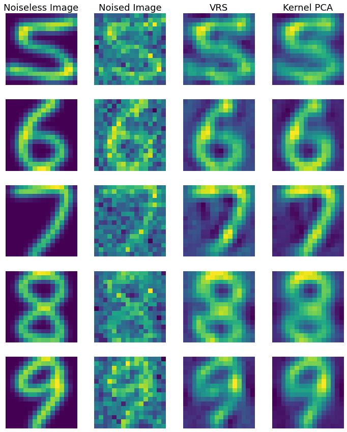
a USPS digits dataset.

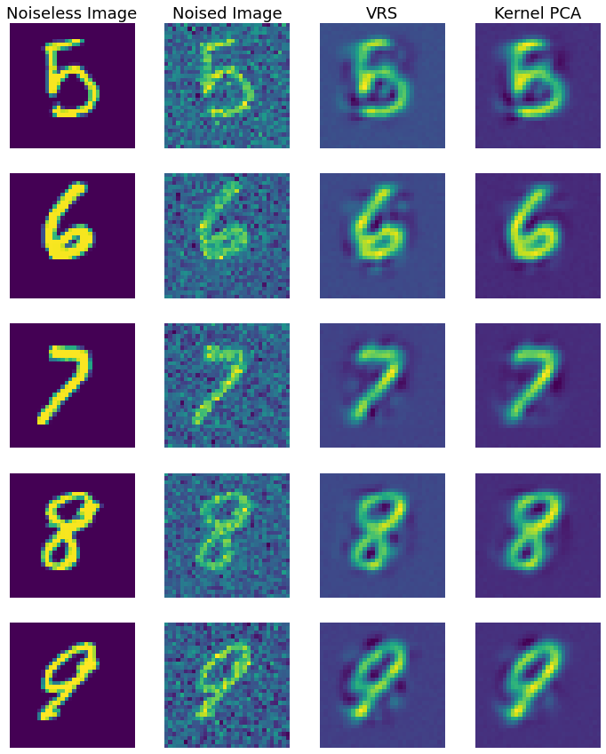
b MNIST dataset.

Figure 8: Denoising images from (a) USPS digits dataset and (b) MNIST dataset. In both (a) and (b), the first column shows the ground truth images from the test data, the second column shows the images polluted by Gaussian noise, the third column shows the images denoised using VRS, and the last column shows the images denoised using kernel PCA.

References

- Al Daas et al. (2023) Hussam Al Daas, Grey Ballard, Paul Cazeaux, Eric Hallman, Agnieszka Miedlar, Mirjeta Pasha, Tim W Reid, and Arvind K Saibaba. Randomized algorithms for rounding in the tensor-train format. SIAM Journal on Scientific Computing, 45(1):A74–A95, 2023.
- Alaoui and Mahoney (2015) Ahmed Alaoui and Michael W Mahoney. Fast randomized kernel ridge regression with statistical guarantees. Advances in neural information processing systems, 28, 2015.
- Bakır et al. (2004) Gökhan H Bakır, Jason Weston, and Bernhard Schölkopf. Learning to find pre-images. Advances in neural information processing systems, 16:449–456, 2004.
- Bell (2014) Jordan Bell. The singular value decomposition of compact operators on hilbert spaces, 2014.
- Blei et al. (2017) David M Blei, Alp Kucukelbir, and Jon D McAuliffe. Variational inference: A review for statisticians. Journal of the American statistical Association, 112(518):859–877, 2017.
- Candes and Plan (2010) Emmanuel J Candes and Yaniv Plan. Matrix completion with noise. Proceedings of the IEEE, 98(6):925–936, 2010.
- Che and Wei (2019) Maolin Che and Yimin Wei. Randomized algorithms for the approximations of tucker and the tensor train decompositions. Advances in Computational Mathematics, 45(1):395–428, 2019.
- Chen and Khoo (2023) Yian Chen and Yuehaw Khoo. Combining particle and tensor-network methods for partial differential equations via sketching. arXiv preprint arXiv:2305.17884, 2023.
- Chen et al. (2021) Yuxin Chen, Yuejie Chi, Jianqing Fan, Cong Ma, et al. Spectral methods for data science: A statistical perspective. Foundations and Trends® in Machine Learning, 14(5):566–806, 2021.
- Drineas and Mahoney (2016) Petros Drineas and Michael W Mahoney. Randnla: randomized numerical linear algebra. Communications of the ACM, 59(6):80–90, 2016.
- Germain et al. (2015) Mathieu Germain, Karol Gregor, Iain Murray, and Hugo Larochelle. Made: Masked autoencoder for distribution estimation. In International conference on machine learning, pages 881–889. PMLR, 2015.
- Halko et al. (2011) Nathan Halko, Per-Gunnar Martinsson, and Joel A Tropp. Finding structure with randomness: Probabilistic algorithms for constructing approximate matrix decompositions. SIAM review, 53(2):217–288, 2011.
- Hofmann et al. (2008) Thomas Hofmann, Bernhard Schölkopf, and Alexander J Smola. Kernel methods in machine learning. The Annals of Statistics, 36(3):1171–1220, 2008.
- Horn and Johnson (1994) Roger A Horn and Charles R Johnson. Topics in matrix analysis. Cambridge university press, 1994.
- Hur et al. (2023) Yoonhaeng Hur, Jeremy G Hoskins, Michael Lindsey, E Miles Stoudenmire, and Yuehaw Khoo. Generative modeling via tensor train sketching. Applied and Computational Harmonic Analysis, 67:101575, 2023.
- Kingma and Ba (2014) Diederik P Kingma and Jimmy Ba. Adam: A method for stochastic optimization. arXiv preprint arXiv:1412.6980, 2014.
- Kressner et al. (2023) Daniel Kressner, Bart Vandereycken, and Rik Voorhaar. Streaming tensor train approximation. SIAM Journal on Scientific Computing, 45(5):A2610–A2631, 2023.
- Kumar et al. (2012) Sanjiv Kumar, Mehryar Mohri, and Ameet Talwalkar. Sampling methods for the nyström method. The Journal of Machine Learning Research, 13(1):981–1006, 2012.
- Lanzante (1996) John R Lanzante. Resistant, robust and non-parametric techniques for the analysis of climate data: Theory and examples, including applications to historical radiosonde station data. International Journal of Climatology: A Journal of the Royal Meteorological Society, 16(11):1197–1226, 1996.
- Li and Racine (2023) Qi Li and Jeffrey Scott Racine. Nonparametric econometrics: theory and practice. Princeton University Press, 2023.
- Liberty et al. (2007) Edo Liberty, Franco Woolfe, Per-Gunnar Martinsson, Vladimir Rokhlin, and Mark Tygert. Randomized algorithms for the low-rank approximation of matrices. Proceedings of the National Academy of Sciences, 104(51):20167–20172, 2007.
- Liu et al. (2007) Han Liu, John Lafferty, and Larry Wasserman. Sparse nonparametric density estimation in high dimensions using the rodeo. In Artificial Intelligence and Statistics, pages 283–290. PMLR, 2007.
- MacFarland et al. (2016) Thomas W MacFarland, Jan M Yates, et al. Introduction to nonparametric statistics for the biological sciences using R. Springer, 2016.
- Mahoney et al. (2011) Michael W Mahoney et al. Randomized algorithms for matrices and data. Foundations and Trends® in Machine Learning, 3(2):123–224, 2011.
- Martinsson (2019) Per-Gunnar Martinsson. Randomized methods for matrix computations. The Mathematics of Data, 25(4):187–231, 2019.
- Martinsson and Tropp (2020) Per-Gunnar Martinsson and Joel A Tropp. Randomized numerical linear algebra: Foundations and algorithms. Acta Numerica, 29:403–572, 2020.
- Mika et al. (1998) Sebastian Mika, Bernhard Schölkopf, Alex Smola, Klaus-Robert Müller, Matthias Scholz, and Gunnar Rätsch. Kernel pca and de-noising in feature spaces. Advances in neural information processing systems, 11, 1998.
- Minster et al. (2020) Rachel Minster, Arvind K Saibaba, and Misha E Kilmer. Randomized algorithms for low-rank tensor decompositions in the tucker format. SIAM Journal on Mathematics of Data Science, 2(1):189–215, 2020.
- Mohideen et al. (2008) S Kother Mohideen, S Arumuga Perumal, and M Mohamed Sathik. Image de-noising using discrete wavelet transform. International Journal of Computer Science and Network Security, 8(1):213–216, 2008.
- Nakatsukasa and Tropp (2021) Yuji Nakatsukasa and Joel A Tropp. Fast & accurate randomized algorithms for linear systems and eigenvalue problems. arXiv preprint arXiv:2111.00113, 2021.
- Papamakarios et al. (2017) George Papamakarios, Theo Pavlakou, and Iain Murray. Masked autoregressive flow for density estimation. Advances in neural information processing systems, 30, 2017.
- Peng et al. (2023) Yifan Peng, Yian Chen, E Miles Stoudenmire, and Yuehaw Khoo. Generative modeling via hierarchical tensor sketching. arXiv preprint arXiv:2304.05305, 2023.
- Pope et al. (2021) Phillip Pope, Chen Zhu, Ahmed Abdelkader, Micah Goldblum, and Tom Goldstein. The intrinsic dimension of images and its impact on learning. arXiv preprint arXiv:2104.08894, 2021.
- Rahimi and Recht (2007) Ali Rahimi and Benjamin Recht. Random features for large-scale kernel machines. Advances in neural information processing systems, 20, 2007.
- Raskutti and Mahoney (2016) Garvesh Raskutti and Michael W Mahoney. A statistical perspective on randomized sketching for ordinary least-squares. The Journal of Machine Learning Research, 17(1):7508–7538, 2016.
- Raskutti et al. (2012) Garvesh Raskutti, Martin J Wainwright, and Bin Yu. Minimax-optimal rates for sparse additive models over kernel classes via convex programming. Journal of machine learning research, 13(2), 2012.
- Ravikumar et al. (2009) Pradeep Ravikumar, John Lafferty, Han Liu, and Larry Wasserman. Sparse additive models. Journal of the Royal Statistical Society Series B: Statistical Methodology, 71(5):1009–1030, 2009.
- Sande et al. (2020) Espen Sande, Carla Manni, and Hendrik Speleers. Explicit error estimates for spline approximation of arbitrary smoothness in isogeometric analysis. Numerische Mathematik, 144(4):889–929, 2020.
- Schmidt-hieber (2020) Johannes Schmidt-hieber. Nonparametric regression using deep neural networks with relu activation function. The Annals of Statistics, 48(4):1875–1897, 2020.
- Shi et al. (2023) Tianyi Shi, Maximilian Ruth, and Alex Townsend. Parallel algorithms for computing the tensor-train decomposition. SIAM Journal on Scientific Computing, 45(3):C101–C130, 2023.
- Sun et al. (2020) Yiming Sun, Yang Guo, Charlene Luo, Joel Tropp, and Madeleine Udell. Low-rank tucker approximation of a tensor from streaming data. SIAM Journal on Mathematics of Data Science, 2(4):1123–1150, 2020.
- Tang and Ying (2023) Xun Tang and Lexing Ying. Solving high-dimensional fokker-planck equation with functional hierarchical tensor. arXiv preprint arXiv:2312.07455, 2023.
- Tang et al. (2022) Xun Tang, Yoonhaeng Hur, Yuehaw Khoo, and Lexing Ying. Generative modeling via tree tensor network states. arXiv preprint arXiv:2209.01341, 2022.
- Tropp et al. (2017a) Joel A Tropp, Alp Yurtsever, Madeleine Udell, and Volkan Cevher. Fixed-rank approximation of a positive-semidefinite matrix from streaming data. Advances in Neural Information Processing Systems, 30, 2017a.
- Tropp et al. (2017b) Joel A Tropp, Alp Yurtsever, Madeleine Udell, and Volkan Cevher. Practical sketching algorithms for low-rank matrix approximation. SIAM Journal on Matrix Analysis and Applications, 38(4):1454–1485, 2017b.
- Ullah and Pagan (1999) Aman Ullah and Adrian Pagan. Nonparametric econometrics. Cambridge university press Cambridge, 1999.
- Uria et al. (2016) Benigno Uria, Marc-Alexandre Côté, Karol Gregor, Iain Murray, and Hugo Larochelle. Neural autoregressive distribution estimation. The Journal of Machine Learning Research, 17(1):7184–7220, 2016.
- Vershynin (2018) Roman Vershynin. High-dimensional probability: An introduction with applications in data science, volume 47. Cambridge university press, 2018.
- Wainwright (2019) Martin J Wainwright. High-dimensional statistics: A non-asymptotic viewpoint, volume 48. Cambridge university press, 2019.
- Wang et al. (2017) Shusen Wang, Alex Gittens, and Michael W Mahoney. Sketched ridge regression: Optimization perspective, statistical perspective, and model averaging. In International Conference on Machine Learning, pages 3608–3616. PMLR, 2017.
- Wasserman (2006) Larry Wasserman. All of nonparametric statistics. Springer Science & Business Media, 2006.
- Williams and Seeger (2000) Christopher Williams and Matthias Seeger. Using the nyström method to speed up kernel machines. Advances in neural information processing systems, 13, 2000.
- Woodruff et al. (2014) David P Woodruff et al. Sketching as a tool for numerical linear algebra. Foundations and Trends® in Theoretical Computer Science, 10(1–2):1–157, 2014.
- Xu (2018) Yuan Xu. Approximation by polynomials in sobolev spaces with jacobi weight. Journal of Fourier Analysis and Applications, 24:1438–1459, 2018.
- Yang et al. (2017) Yun Yang, Mert Pilanci, and Martin J Wainwright. Randomized sketches for kernels: Fast and optimal nonparametric regression. Annals of Statistics, pages 991–1023, 2017.
- Yuan and Zhou (2016) Ming Yuan and Ding-Xuan Zhou. Minimax optimal rates of estimation in high dimensional additive models. Annals of Statistics, 44(6):2564–2593, 2016.
- Zhang et al. (2015) Yuchen Zhang, John Duchi, and Martin Wainwright. Divide and conquer kernel ridge regression: A distributed algorithm with minimax optimal rates. The Journal of Machine Learning Research, 16(1):3299–3340, 2015.