New physics search via angular distribution of Bβ†’Dβˆ—β€‹β„“β€‹Ξ½β„“β†’π΅superscript𝐷ℓsubscriptπœˆβ„“B\to D^{*}\ell\nu_{\ell} decay in the light of the new lattice data

Tejhas Kapoor tejhas.kapoor@ijclab.in2p3.fr UniversitΓ© Paris-Saclay, CNRS/IN2P3, IJCLab, 91405 Orsay, France Zhuo-Ran Huang Department of Physics, College of Physics, Mechanical and Electrical Engineering, Jishou University, Jishou 416000, China Emi Kou UniversitΓ© Paris-Saclay, CNRS/IN2P3, IJCLab, 91405 Orsay, France
Abstract

In this article, we investigate the angular distribution of the Bβ†’Dβˆ—β€‹β„“β€‹Ξ½β„“β†’π΅superscript𝐷ℓsubscriptπœˆβ„“{B}\to D^{*}\ell{\nu}_{\ell}\;process to search for New Physics signals. The Belle collaboration has analysed it to constraint Vc​bsubscript𝑉𝑐𝑏V_{cb} and the Bβ†’Dβˆ—β†’π΅superscript𝐷B\to D^{*} form factors, under the assumption of the Standard Model. With the newly released lattice QCD data, we can perform a simultaneous fit of the form factors, Vc​bsubscript𝑉𝑐𝑏V_{cb} as well as of furthermore new physics parameters. We use the untagged Belle data and the lattice data to constrain right-handed new physics. In addition, we also generate unbinned pseudo-dataset and perform a sensitivity study on more general new physics models, along with the lattice data.

1 Introduction

The Bβ†’Dβˆ—β€‹β„“β€‹Ξ½β„“β†’π΅superscript𝐷ℓsubscriptπœˆβ„“{B}\to D^{*}\ell{\nu}_{\ell}\;decay has been paid a great attention in recent years. The first reason for this is the Vc​bsubscript𝑉𝑐𝑏V_{cb} puzzle: there has been a longstanding tension between the values of |Vc​b|subscript𝑉𝑐𝑏|V_{cb}| determined using the inclusive measurements and that determined by the exclusive bβ†’cβ€‹β„“β€‹Ξ½β†’π‘π‘β„“πœˆb\rightarrow c\ell\nu decays. The inclusive measurement uses the semileptonic decays of the type Bβ†’Xc​ℓ​ν→𝐡subscriptπ‘‹π‘β„“πœˆB\rightarrow X_{c}\ell\nu, where Xcsubscript𝑋𝑐X_{c} are all possible hadronic states including charm quark. The current world average is |Vc​b|=(42.2Β±0.8)Γ—10βˆ’3subscript𝑉𝑐𝑏plus-or-minus42.20.8superscript103|V_{cb}|=(42.2\pm 0.8)\times 10^{-3}Β [1]. On the other hand, the exclusive measurement of |Vc​b|subscript𝑉𝑐𝑏|V_{cb}| has the following world average: |Vc​b|=(38.46Β±0.40Β±0.55)Γ—10βˆ’3subscript𝑉𝑐𝑏plus-or-minus38.460.400.55superscript103{\color[rgb]{0,0,0}|V_{cb}|=}(38.46\pm 0.40\pm 0.55)\times 10^{-3}, where the first uncertainty combines the statistical and systematic uncertainties from the experimental measurement and the second is theoretical (lattice QCD calculation and electroweak correction) [2].

The second reason is the so-called ℛ​(D(βˆ—))β„›superscript𝐷\mathcal{R}(D^{(*)}) anomaly: to test the lepton flavour universality in the bβ†’cβ€‹β„“β€‹Ξ½β†’π‘π‘β„“πœˆb\rightarrow c\ell\nu decays, a ratio is defined:

ℛ​(D(βˆ—))=ℬ​(Bβ†’D(βˆ—)​τ​ν)ℬ​(Bβ†’D(βˆ—)​ℓ​ν);β„“={e,ΞΌ}formulae-sequenceβ„›superscript𝐷ℬ→𝐡superscriptπ·πœπœˆβ„¬β†’π΅superscriptπ·β„“πœˆβ„“π‘’πœ‡\displaystyle\mathcal{R}(D^{(*)})=\frac{\mathcal{B}(B\rightarrow D^{(*)}\tau\nu)}{\mathcal{B}(B\rightarrow D^{(*)}\ell\nu)};\quad\ell=\{e,\mu\} (1)

The combined results from BaBarΒ [3, 4], BelleΒ [5, 6, 7, 8], LHCbΒ [9, 10] and Belle IIΒ [11] exceed the SM predictionsΒ [2] by about 3.3​σ3.3𝜎3.3\sigma. Theoretical efforts to explain such anomalies branch into model-independent and model-dependent analysis. For the model-dependent analysis, several classes of models have been proposed to provide a resolution to such anomalies. These classes of models can be divided into three major categories: extended higgs sector models [12, 13, 14, 15, 16, 17, 18, 19, 20, 21], heavy charged vector boson models [22, 23, 24, 25, 26, 27] and leptoquark models [28, 29, 30, 31, 32, 33], with the latter being the most popularΒ [34]. Given that the ratio ℛ​(D(βˆ—))β„›superscript𝐷\mathcal{R}(D^{(*)}) is measured to be higher than its SM prediction, the model-dependent approaches usually try to enhance the Bβ†’D(βˆ—)​τ​ν→𝐡superscript𝐷𝜏𝜈B\rightarrow D^{(*)}\tau\nu rate (say, by introducing new heavy particles), rather than suppress the Bβ†’D(βˆ—)​ℓ​ν→𝐡superscriptπ·β„“πœˆB\rightarrow D^{(*)}\ell\nu rate, as the latter have stringent constraints on new physics coupling to electrons and muonsΒ [35].

In this work, we explore the potential of the angular distribution analysis of the Bβ†’Dβˆ—β€‹β„“β€‹Ξ½β„“β†’π΅superscript𝐷ℓsubscriptπœˆβ„“{B}\to D^{*}\ell{\nu}_{\ell}\;process (β„“=e,ΞΌβ„“π‘’πœ‡\ell=e,\mu) to search for signals beyond the SM, following the model-independent approach. We will work with a low-energy effective Hamiltonian containing all dimension six, four-fermion operators, assuming no right-handed neutrinos. We expect the angular distribution to be a powerful tool to distinguish the different Dirac structure that these operators have: (left)right-handed, (pseudo)scalar and tensor. These contributions can arise in several NP scenarios. For example, the right-handed contribution can arise from WLβˆ’WRsubscriptπ‘ŠπΏsubscriptπ‘Šπ‘…W_{L}-W_{R} mixing left-right symmetric modelsΒ [36, 37, 38, 39, 40, 41, 42, 43, 44, 45, 46, 47, 48]. On the other hand, the scalar contribution is generated in models with extra charged scalarsΒ [49, 50, 51, 52, 53, 54, 55, 56, 57, 58, 59, 60], while the tensor operators are often generated by a Fierz transformation on scalar operators [34]. These NP effects can be both lepton flavour universal and lepton flavour violating, thus, having strong implication on the R​(D(βˆ—))𝑅superscript𝐷R(D^{(*)}) anomaly.

Belle has used the angular distribution data of Bβ†’Dβˆ—β€‹β„“β€‹Ξ½β„“β†’π΅superscript𝐷ℓsubscriptπœˆβ„“{B}\to D^{*}\ell{\nu}_{\ell}\;decay to fit simultaneously |Vc​b|subscript𝑉𝑐𝑏|V_{cb}| and the form factorsΒ [61, 62, 63]. The angular distribution is written in terms of 4 kinematical variables (one invariant mass and three angles). The analysis uses four, one-dimensional binned distributions (corresponding to each kinematical variable), in which the other three variables are integrated away. Since |Vc​b|subscript𝑉𝑐𝑏|V_{cb}| is always multiplied with a scaling factor ℱ​(w)​ηEWℱ𝑀subscriptπœ‚EW\mathcal{F}(w)\eta_{\rm EW}, the fit parameter is actually |Vc​b|​ℱ​(1)​ηEWsubscript𝑉𝑐𝑏ℱ1subscriptπœ‚EW|V_{cb}|\mathcal{F}(1)\eta_{\rm EW}, where Ξ·EWsubscriptπœ‚EW\eta_{\rm EW} is the electroweak correction, and ℱ​(1)=hA1​(1)β„±1subscriptβ„Žsubscript𝐴11\mathcal{F}(1)=h_{A_{1}}(1) is a form factor at zero-recoil. Therefore, the value of ℱ​(1)β„±1\mathcal{F}(1) is required to obtain |Vc​b|subscript𝑉𝑐𝑏|V_{cb}|. It should be noted that addition of NP effects increases the number of parameters, and experimental data alone cannot fit form factors, Vc​bsubscript𝑉𝑐𝑏V_{cb} and NP parameters simultaneously.

The recent lattice QCD results from Fermilab-MILC[64], JLQCD[65] and HPQCD collaborations [66] provided a breakthrough, by publishing the results on the form factors for this decay. Previously, only ℱ​(1)β„±1\mathcal{F}(1) was known at zero recoil; but now we have results on four form factors (f,g,β„±1,β„±2)𝑓𝑔subscriptβ„±1subscriptβ„±2(f,g,\mathcal{F}_{1},\mathcal{F}_{2}) in the low-recoil region. In the light of these new results, we present a simultaneous fit of Belle and lattice QCD data. Now, thanks to the lattice data, we can even fit the NP parameters, allowing us to constrain different types of NP. In addition to using the Belle binned dataset, we will also demonstrate the fit using an unbinned belle pseudo datasetΒ [67] – the latter will become possible once a larger amount of data becomes available at the Belle II experimentΒ [68].

The organisation of the article is as follows: In SectionΒ 2 we introduce the effective Hamiltonian and the different NP operators relevant for the Bβ†’Dβˆ—β€‹β„“β€‹Ξ½β„“β†’π΅superscript𝐷ℓsubscriptπœˆβ„“{B}\to D^{*}\ell{\nu}_{\ell}\;decay. In SectionΒ 3, we write the complete angular decay distribution for the Bβ†’Dβˆ—β€‹β„“β€‹Ξ½β„“β†’π΅superscript𝐷ℓsubscriptπœˆβ„“{B}\to D^{*}\ell{\nu}_{\ell}\;process in terms of the NP Wilson coefficients, hadronic and leptonic amplitudes. In SectionΒ 4, we describe the new lattice QCD data in the BGL form factor parameteriation, and show the form factor fit results to the higher recoil region using the new lattice data. In SectionΒ 5, we use the untagged Belle binned data along with the lattice data to fit form factors, Vc​bsubscript𝑉𝑐𝑏V_{cb} and right-handed NP Wilson coefficient, and present the fit results. Finally, in SectionΒ 6, we demonstrate the fit procedure with unbinned Belle and lattice data and perform a sensitivity study with different NP operators and we conclude in SedctionΒ 7

2 New physics model

In this article, we consider the new physics particle which contributes to the semi-leptonic Bβ†’Dβˆ—β€‹β„“β€‹Ξ½β„“β†’π΅superscript𝐷ℓsubscriptπœˆβ„“{B}\to D^{*}\ell{\nu}_{\ell}\;decay with β„“=e,ΞΌβ„“π‘’πœ‡\ell=e,\mu. We start with the most general effective Hamiltonian, containing all dimension six, four-fermion operators, assuming no right-handed neutrinos:

β„‹eff=4​GF2​Vc​bβ€‹βˆ‘β„“=e,ΞΌ[CVLℓ​OVLβ„“+CVRℓ​OVRβ„“+CSℓ​OSβ„“+CPℓ​OPβ„“+CTℓ​OTβ„“]subscriptβ„‹eff4subscript𝐺𝐹2subscript𝑉𝑐𝑏subscriptβ„“π‘’πœ‡delimited-[]superscriptsubscript𝐢subscriptVLβ„“subscriptsuperscript𝑂ℓsubscriptVLsuperscriptsubscript𝐢subscriptVRβ„“subscriptsuperscript𝑂ℓsubscriptVRsuperscriptsubscript𝐢Sβ„“subscriptsuperscript𝑂ℓSsuperscriptsubscript𝐢Pβ„“subscriptsuperscript𝑂ℓPsuperscriptsubscript𝐢Tβ„“subscriptsuperscript𝑂ℓT\mathcal{H}_{\rm eff}=\frac{4G_{F}}{\sqrt{2}}V_{cb}\sum_{\ell=e,\mu}[C_{\rm V_{L}}^{\ell}O^{\ell}_{\rm V_{L}}+C_{\rm V_{R}}^{\ell}O^{\ell}_{\rm V_{R}}+{C_{\rm S}^{\ell}O^{\ell}_{\rm S}}+C_{\rm P}^{\ell}O^{\ell}_{\rm P}+C_{\rm T}^{\ell}O^{\ell}_{\rm T}] (2)

where VL,VR,S,P,TsubscriptVLsubscriptVRSPT{\rm V_{L},V_{R},S,P,T} indicate the left-handed, right-handed, scalar, pseudoscalar, and tensor terms, respectively. The corresponding operators are given as

OVLβ„“=(cΒ―L​γμ​bL)​(β„“Β―L​γμ​νℓ​L)OVRβ„“=(cΒ―R​γμ​bR)​(β„“Β―L​γμ​νℓ​L)OSβ„“=(c¯​b)​(β„“Β―R​νℓ​L)OPβ„“=(c¯​γ5​b)​(β„“Β―R​νℓ​L)OTβ„“=(cΒ―R​σμ​ν​bL)​(β„“Β―R​σμ​ν​νℓ​L)subscriptsuperscript𝑂ℓsubscriptVLabsentsubscript¯𝑐𝐿superscriptπ›Ύπœ‡subscript𝑏𝐿subscript¯ℓ𝐿subscriptπ›Ύπœ‡subscriptπœˆβ„“πΏsubscriptsuperscript𝑂ℓsubscriptVRabsentsubscript¯𝑐𝑅superscriptπ›Ύπœ‡subscript𝑏𝑅subscript¯ℓ𝐿subscriptπ›Ύπœ‡subscriptπœˆβ„“πΏsubscriptsuperscript𝑂ℓSabsent¯𝑐𝑏subscript¯ℓ𝑅subscriptπœˆβ„“πΏsubscriptsuperscript𝑂ℓPabsent¯𝑐superscript𝛾5𝑏subscript¯ℓ𝑅subscriptπœˆβ„“πΏsubscriptsuperscript𝑂ℓTabsentsubscript¯𝑐𝑅superscriptπœŽπœ‡πœˆsubscript𝑏𝐿subscript¯ℓ𝑅subscriptπœŽπœ‡πœˆsubscriptπœˆβ„“πΏ\displaystyle\begin{aligned} O^{\ell}_{\rm V_{L}}&=(\bar{c}_{L}\gamma^{\mu}b_{L})(\bar{{\ell}}_{L}\gamma_{\mu}\nu_{{\ell}L})\\ O^{\ell}_{\rm V_{R}}&=(\bar{c}_{R}\gamma^{\mu}b_{R})(\bar{{\ell}}_{L}\gamma_{\mu}\nu_{{\ell}L})\\ O^{\ell}_{\rm S}&=(\bar{c}b)(\bar{{\ell}}_{R}\nu_{{\ell}L})\\ O^{\ell}_{\rm P}&=(\bar{c}\gamma^{5}b)(\bar{{\ell}}_{R}\nu_{{\ell}L})\\ O^{\ell}_{\rm T}&=(\bar{c}_{R}\sigma^{\mu\nu}b_{L})(\bar{{\ell}}_{R}\sigma_{\mu\nu}\nu_{{\ell}L})\end{aligned} (3)

where ψL/R=1βˆ“Ξ³52β€‹Οˆsubscriptπœ“πΏπ‘…minus-or-plus1subscript𝛾52πœ“\psi_{L/R}=\frac{1\mp\gamma_{5}}{2}\psi with ψ={c,b,β„“,Ξ½}πœ“π‘π‘β„“πœˆ\psi=\{c,b,\ell,\nu\}. The contribution from the scalar operator OSβ„“subscriptsuperscript𝑂ℓSO^{\ell}_{\rm S} does not appear in the following. We ignore the superscript β„“β„“\ell in the following discussion. In the SM, CVL=1subscript𝐢subscriptVL1C_{\rm V_{L}}=1, while the rest of the Wilson coefficients are zero.

3 Angular distribution of the Bβ†’Dβˆ—β€‹β„“β€‹Ξ½β„“β†’π΅superscript𝐷ℓsubscriptπœˆβ„“{B}\to D^{*}\ell{\nu}_{\ell}\;decay

Using the Hamiltonian given in Eq.Β (2), we compute the the angular distribution of the Bβ†’Dβˆ—β€‹β„“β€‹Ξ½β„“β†’π΅superscript𝐷ℓsubscriptπœˆβ„“{B}\to D^{*}\ell{\nu}_{\ell}\;decay (shown in Fig.Β 1):

dΞ“(BΒ―β†’Dβˆ—(β†’DΟ€)β„“βˆ’Ξ½Β―β„“)d​q2​d​cos⁑θV​d​cos⁑θℓ​d​χ=38​(4​π)4​(q2βˆ’mβ„“2)2​|pβ†’Dβˆ—|2MB2​q2​GF2​|Vc​b|2​|Ξ·EW|2​ℬ​(Dβˆ—β†’D​π)βˆ‘Ξ»β„“,λνℓ|β„³VL+β„³VR+β„³P+β„³T|2\displaystyle\begin{aligned} \frac{\text{d}\Gamma(\bar{B}\to D^{*}(\to D\pi)\,\ell^{-}\,\bar{\nu}_{\ell})}{\text{d}q^{2}\,\text{d}\cos\theta_{V}\,\text{d}\cos\theta_{\ell}\,\text{d}\chi}=&\frac{3}{8(4\pi)^{4}}\frac{(q^{2}-m_{\ell}^{2})^{2}|\vec{p}_{D^{*}}|^{2}}{M_{B}^{2}q^{2}}G_{F}^{2}|V_{cb}|^{2}|\eta_{\rm EW}|^{2}\mathcal{B}(D^{*}\rightarrow D\pi)\\ &\sum_{\lambda_{\ell},\lambda_{\nu_{\ell}}}|\mathcal{M}_{\rm V_{L}}+\mathcal{M}_{\rm V_{R}}+\mathcal{M}_{\rm P}+\mathcal{M}_{\rm T}|^{2}\end{aligned} (4)
Refer to caption
Figure 1: Decay angles for the Bβ†’Dβˆ—β€‹β„“β€‹Ξ½β„“β†’π΅superscript𝐷ℓsubscriptπœˆβ„“{B}\to D^{*}\ell{\nu}_{\ell}\;decay, where ΞΈVsubscriptπœƒπ‘‰\theta_{V} is the angle between the direction of D𝐷D meson and the direction opposite to that of B𝐡B meson, in the Dβˆ—superscript𝐷D^{*} meson rest frame. Similarly, ΞΈβ„“subscriptπœƒβ„“\theta_{\ell} is the angle between the direction of lepton and the direction opposite to that of B𝐡B meson, in the virtual Wπ‘ŠW rest frame. Ο‡πœ’\chi is the angle between the two decay planes.

where q2superscriptπ‘ž2q^{2} is the invariant mass of the lepton-neutrino pair. Following the method given inΒ [69], we compute the amplitudes β„³VL,VR,P,Tsubscriptβ„³subscriptVLsubscriptVRPT\mathcal{M}_{\rm V_{L},V_{R},P,T}. In this method, we introduce the Wπ‘ŠW boson polarisation and separate the amplitudes into the hadronic and leptonic part as:

β„³VL=CVLβ€‹βˆ‘Ξ»Dβˆ—=Β±,0P​(Ξ»Dβˆ—)β€‹βˆ‘Ξ»=t,Β±,0gλ​λ​HVL,λλDβˆ—β€‹LΞ»VAβ„³VR=CVRβ€‹βˆ‘Ξ»Dβˆ—=Β±,0P​(Ξ»Dβˆ—)β€‹βˆ‘Ξ»=t,Β±,0gλ​λ​HVR,λλDβˆ—β€‹LΞ»VAβ„³P=CPβ€‹βˆ‘Ξ»Dβˆ—=Β±,0P​(Ξ»Dβˆ—)​HPΞ»Dβˆ—β€‹LSPβ„³T=CTβ€‹βˆ‘Ξ»Dβˆ—=Β±,0P​(Ξ»Dβˆ—)β€‹βˆ‘Ξ»=t,Β±,0βˆ‘Ξ»β€²=t,Β±,0gλ​λ​gλ′​λ′​HT,λ​λ′λDβˆ—β€‹Lλ​λ′Tsubscriptβ„³subscriptVLabsentsubscript𝐢subscriptVLsubscriptsubscriptπœ†superscript𝐷plus-or-minus0𝑃subscriptπœ†superscript𝐷subscriptπœ†π‘‘plus-or-minus0subscriptπ‘”πœ†πœ†subscriptsuperscript𝐻subscriptπœ†superscript𝐷subscriptVLπœ†superscriptsubscriptπΏπœ†VAsubscriptβ„³subscriptVRabsentsubscript𝐢subscriptVRsubscriptsubscriptπœ†superscript𝐷plus-or-minus0𝑃subscriptπœ†superscript𝐷subscriptπœ†π‘‘plus-or-minus0subscriptπ‘”πœ†πœ†subscriptsuperscript𝐻subscriptπœ†superscript𝐷subscriptVRπœ†superscriptsubscriptπΏπœ†VAsubscriptβ„³Pabsentsubscript𝐢Psubscriptsubscriptπœ†superscript𝐷plus-or-minus0𝑃subscriptπœ†superscript𝐷subscriptsuperscript𝐻subscriptπœ†superscript𝐷Psuperscript𝐿SPsubscriptβ„³Tabsentsubscript𝐢Tsubscriptsubscriptπœ†superscript𝐷plus-or-minus0𝑃subscriptπœ†superscript𝐷subscriptπœ†π‘‘plus-or-minus0subscriptsuperscriptπœ†β€²π‘‘plus-or-minus0subscriptπ‘”πœ†πœ†subscript𝑔superscriptπœ†β€²superscriptπœ†β€²subscriptsuperscript𝐻subscriptπœ†superscript𝐷Tπœ†superscriptπœ†β€²subscriptsuperscript𝐿Tπœ†superscriptπœ†β€²\displaystyle\begin{aligned} \mathcal{M}_{\rm V_{L}}&=\,C_{\rm V_{L}}\sum_{\lambda_{D^{*}}=\pm,0}P(\lambda_{D^{*}})\sum_{\lambda=t,\pm,0}g_{\lambda\lambda}H^{\lambda_{D^{*}}}_{\rm V_{L},\lambda}L_{\lambda}^{\rm VA}\\ \mathcal{M}_{\rm V_{R}}&=\,C_{\rm V_{R}}\sum_{\lambda_{D^{*}}=\pm,0}P(\lambda_{D^{*}})\sum_{\lambda=t,\pm,0}g_{\lambda\lambda}H^{\lambda_{D^{*}}}_{\rm V_{R},\lambda}L_{\lambda}^{\rm VA}\\ \mathcal{M}_{\rm P}&=\,C_{\rm P}\sum_{\lambda_{D^{*}}=\pm,0}P(\lambda_{D^{*}})H^{\lambda_{D^{*}}}_{\rm P}L^{\rm SP}\\ \mathcal{M}_{\rm T}&=\,C_{\rm T}\sum_{\lambda_{D^{*}}=\pm,0}P(\lambda_{D^{*}})\sum_{\lambda=t,\pm,0}\sum_{\lambda^{\prime}=t,\pm,0}g_{\lambda\lambda}g_{\lambda^{\prime}\lambda^{\prime}}H^{\lambda_{D^{*}}}_{\rm T,\lambda\lambda^{\prime}}L^{\rm T}_{\lambda\lambda^{\prime}}\end{aligned} (5)

where P​(Ξ»Dβˆ—)=⟨D​π|Dβˆ—βŸ©=2​g​ϡDβˆ—βˆ—Ξ±β€‹(Ξ»Dβˆ—)​pD,α𝑃subscriptπœ†superscript𝐷inner-productπ·πœ‹superscript𝐷2𝑔superscriptsubscriptitalic-Ο΅superscript𝐷absent𝛼subscriptπœ†superscript𝐷subscript𝑝𝐷𝛼P(\lambda_{D^{*}})=\langle D\pi|D^{*}\rangle=2g\epsilon_{D^{*}}^{*\alpha}(\lambda_{D^{*}})p_{D,\alpha} (g𝑔g is the Dβˆ—superscript𝐷D^{*}-D𝐷D-Ο€πœ‹\pi coupling), Ο΅Dβˆ—subscriptitalic-Ο΅superscript𝐷\epsilon_{D^{*}} is the polarisation vector of Dβˆ—superscript𝐷D^{*} meson and Ξ»Dβˆ—βˆˆ{+,βˆ’,0}subscriptπœ†superscript𝐷0\lambda_{D^{*}}\in\{+,-,0\} is the polarisation of Dβˆ—superscript𝐷D^{*} meson. The polarisation vectors are given inΒ [69].

The hadronic amplitudes are given as

HVL,λλDβˆ—β€‹(q2)=Ο΅Β―ΞΌβˆ—β€‹(Ξ»)β€‹βŸ¨Dβˆ—β€‹(pDβˆ—,Ο΅Dβˆ—β€‹(Ξ»Dβˆ—))|c¯​γμ​(1βˆ’Ξ³5)​b|B¯​(pB)⟩,HVR,λλDβˆ—β€‹(q2)=Ο΅Β―ΞΌβˆ—β€‹(Ξ»)β€‹βŸ¨Dβˆ—β€‹(pDβˆ—,Ο΅Dβˆ—β€‹(Ξ»Dβˆ—))|c¯​γμ​(1+Ξ³5)​b|B¯​(pB)⟩,HPΞ»Dβˆ—β€‹(q2)=⟨Dβˆ—β€‹(pDβˆ—,Ο΅Dβˆ—β€‹(Ξ»Dβˆ—))|c¯​γ5​b|B¯​(pB)⟩,HT,λ​λ′λDβˆ—β€‹(q2)=iβ€‹Ο΅Β―ΞΌβˆ—β€‹(Ξ»)β€‹Ο΅Β―Ξ½βˆ—β€‹(Ξ»β€²)β€‹βŸ¨Dβˆ—β€‹(pDβˆ—,ϡ​(Ξ»Dβˆ—))|c¯​σμ​ν​(1βˆ’Ξ³5)​b|B¯​(pB)⟩,superscriptsubscript𝐻subscriptVLπœ†subscriptπœ†superscript𝐷superscriptπ‘ž2absentsubscriptsuperscriptΒ―italic-Ο΅πœ‡πœ†quantum-operator-productsuperscript𝐷subscript𝑝superscript𝐷subscriptitalic-Ο΅superscript𝐷subscriptπœ†superscript𝐷¯𝑐superscriptπ›Ύπœ‡1superscript𝛾5𝑏¯𝐡subscript𝑝𝐡superscriptsubscript𝐻subscriptVRπœ†subscriptπœ†superscript𝐷superscriptπ‘ž2absentsubscriptsuperscriptΒ―italic-Ο΅πœ‡πœ†quantum-operator-productsuperscript𝐷subscript𝑝superscript𝐷subscriptitalic-Ο΅superscript𝐷subscriptπœ†superscript𝐷¯𝑐superscriptπ›Ύπœ‡1superscript𝛾5𝑏¯𝐡subscript𝑝𝐡superscriptsubscript𝐻Psubscriptπœ†superscript𝐷superscriptπ‘ž2absentquantum-operator-productsuperscript𝐷subscript𝑝superscript𝐷subscriptitalic-Ο΅superscript𝐷subscriptπœ†superscript𝐷¯𝑐superscript𝛾5𝑏¯𝐡subscript𝑝𝐡superscriptsubscript𝐻Tπœ†superscriptπœ†β€²subscriptπœ†superscript𝐷superscriptπ‘ž2absent𝑖subscriptsuperscriptΒ―italic-Ο΅πœ‡πœ†subscriptsuperscriptΒ―italic-ϡ𝜈superscriptπœ†β€²quantum-operator-productsuperscript𝐷subscript𝑝superscript𝐷italic-Ο΅subscriptπœ†superscript𝐷¯𝑐superscriptπœŽπœ‡πœˆ1superscript𝛾5𝑏¯𝐡subscript𝑝𝐡\displaystyle\begin{aligned} H_{\rm V_{L},\lambda}^{\lambda_{D^{*}}}(q^{2})&=\bar{\epsilon}^{*}_{\mu}(\lambda)\langle D^{*}(p_{D^{*}},\epsilon_{D^{*}}\left(\lambda_{D^{*}})\right)|\bar{c}\gamma^{\mu}(1-\gamma^{5})b|\bar{B}(p_{B})\rangle\,,\\ H_{\rm V_{R},\lambda}^{\lambda_{D^{*}}}(q^{2})&=\bar{\epsilon}^{*}_{\mu}(\lambda)\langle D^{*}(p_{D^{*}},\epsilon_{D^{*}}\left(\lambda_{D^{*}})\right)|\bar{c}\gamma^{\mu}(1+\gamma^{5})b|\bar{B}(p_{B})\rangle\,,\\ H_{\rm P}^{\lambda_{D^{*}}}(q^{2})&=\langle D^{*}(p_{D^{*}},\epsilon_{D^{*}}\left(\lambda_{D^{*}})\right)|\bar{c}\gamma^{5}b|\bar{B}(p_{B})\rangle\,,\\ H_{\rm T,\lambda\lambda^{\prime}}^{\lambda_{D^{*}}}(q^{2})&=i\bar{\epsilon}^{*}_{\mu}(\lambda)\bar{\epsilon}^{*}_{\nu}(\lambda^{\prime})\langle D^{*}(p_{D^{*}},\epsilon\left(\lambda_{D^{*}})\right)|\bar{c}\sigma^{\mu\nu}(1-\gamma^{5})b|\bar{B}(p_{B})\rangle,\end{aligned} (6)

and the leptonic amplitudes are given as

LΞ»VL/R=ϡ¯μ​(Ξ»)​u¯ℓ​γμ​(1βˆ“Ξ³5)​vΞ½Β―β„“LP=u¯ℓ​(1βˆ’Ξ³5)​vΞ½Β―β„“LΞ»,Ξ»β€²T=βˆ’i​ϡ¯μ​(Ξ»)​ϡ¯ν​(Ξ»β€²)​u¯ℓ​σμ​ν​(1βˆ’Ξ³5)​vΞ½Β―β„“subscriptsuperscript𝐿subscriptVLRπœ†absentsubscriptΒ―italic-Ο΅πœ‡πœ†subscript¯𝑒ℓsuperscriptπ›Ύπœ‡minus-or-plus1superscript𝛾5subscript𝑣subscriptΒ―πœˆβ„“superscript𝐿Pabsentsubscript¯𝑒ℓ1superscript𝛾5subscript𝑣subscriptΒ―πœˆβ„“subscriptsuperscript𝐿Tπœ†superscriptπœ†β€²absent𝑖subscriptΒ―italic-Ο΅πœ‡πœ†subscriptΒ―italic-ϡ𝜈superscriptπœ†β€²subscript¯𝑒ℓsuperscriptπœŽπœ‡πœˆ1superscript𝛾5subscript𝑣subscriptΒ―πœˆβ„“\displaystyle\begin{aligned} L^{\rm V_{L/R}}_{\lambda}&=\bar{\epsilon}_{\mu}(\lambda)\bar{u}_{\ell}\gamma^{\mu}(1\mp\gamma^{5})v_{\bar{\nu}_{\ell}}\\ L^{\rm P}&=\bar{u}_{\ell}(1-\gamma^{5})v_{\bar{\nu}_{\ell}}\\ L^{\rm T}_{\lambda,\lambda^{\prime}}&=-i\bar{\epsilon}_{\mu}(\lambda)\bar{\epsilon}_{\nu}(\lambda^{\prime})\bar{u}_{\ell}\sigma^{\mu\nu}(1-\gamma^{5})v_{\bar{\nu}_{\ell}}\end{aligned} (7)

Both are written by ϡ¯¯italic-Ο΅\bar{\epsilon}, the polarisation vector of Wπ‘ŠW boson, and Ξ»(β€²)∈{+,βˆ’,0,t}\lambda^{(^{\prime})}\in\{+,-,0,t\}, its polarisation. Note that ϡ¯​(t)Β―italic-ϡ𝑑\bar{\epsilon}(t) is not orthogonal but proportional to Wπ‘ŠW-momentum. The polarisation vectors are given in Β [69].

Then, using the completeness relation of the polarisation vectors of Wπ‘ŠW boson, we square the hadronic and leptonic parts of the amplitudes separately. This allows us to evaluate each part in a convenient frame: we choose the Wπ‘ŠW rest frame for the leptonic part and B𝐡B rest frame for the hadronic part.

The hadronic part is a complex function of form factors and we find

HV±​(q2)≑HVL,±±​(q2)=βˆ’HVR,βˆ“βˆ“β€‹(q2)=(MB+MDβˆ—)​A1​(q2)βˆ“Ξ»Dβˆ—β€‹(q2)MB+MDβˆ—β€‹V​(q2)HV0​(q2)≑HVL,00​(q2)=βˆ’HVR,00​(q2)=MB+MDβˆ—2​MDβˆ—β€‹q2​[βˆ’(MB2βˆ’MDβˆ—2βˆ’q2)​A1​(q2)+Ξ»Dβˆ—β€‹(q2)(MB+MDβˆ—)2​A2​(q2)]HP​(q2)≑HP0​(q2)=βˆ’Ξ»Dβˆ—β€‹(q2)MB+mc​A0​(q2)HT±​(q2)≑±HT,Β±t±​(q2)=1q2​[Ξ»Dβˆ—β€‹(q2)​T1​(q2)Β±(MB2βˆ’MDβˆ—2)​T2​(q2)]HT0​(q2)≑HT,+βˆ’0​(q2)=HT,0​t0​(q2)=12​MDβˆ—β€‹[(MB2+3​MDβˆ—2βˆ’q2)​T2​(q2)βˆ’Ξ»Dβˆ—β€‹(q2)(MB2βˆ’MDβˆ—2)​T3​(q2)]superscriptsubscript𝐻Vplus-or-minussuperscriptπ‘ž2absentsuperscriptsubscript𝐻subscriptVLplus-or-minusplus-or-minussuperscriptπ‘ž2superscriptsubscript𝐻subscriptVRminus-or-plusminus-or-plussuperscriptπ‘ž2missing-subexpressionabsentminus-or-plussubscript𝑀𝐡subscript𝑀superscript𝐷subscript𝐴1superscriptπ‘ž2subscriptπœ†superscript𝐷superscriptπ‘ž2subscript𝑀𝐡subscript𝑀superscript𝐷𝑉superscriptπ‘ž2superscriptsubscript𝐻V0superscriptπ‘ž2absentsuperscriptsubscript𝐻subscriptVL00superscriptπ‘ž2superscriptsubscript𝐻subscriptVR00superscriptπ‘ž2missing-subexpressionabsentsubscript𝑀𝐡subscript𝑀superscript𝐷2subscript𝑀superscript𝐷superscriptπ‘ž2delimited-[]superscriptsubscript𝑀𝐡2superscriptsubscript𝑀superscript𝐷2superscriptπ‘ž2subscript𝐴1superscriptπ‘ž2subscriptπœ†superscript𝐷superscriptπ‘ž2superscriptsubscript𝑀𝐡subscript𝑀superscript𝐷2subscript𝐴2superscriptπ‘ž2subscript𝐻Psuperscriptπ‘ž2absentsuperscriptsubscript𝐻P0superscriptπ‘ž2missing-subexpressionabsentsubscriptπœ†superscript𝐷superscriptπ‘ž2subscript𝑀𝐡subscriptπ‘šπ‘subscript𝐴0superscriptπ‘ž2superscriptsubscript𝐻Tplus-or-minussuperscriptπ‘ž2absentplus-or-minussuperscriptsubscript𝐻Tplus-or-minustplus-or-minussuperscriptπ‘ž2missing-subexpressionabsent1superscriptπ‘ž2delimited-[]plus-or-minussubscriptπœ†superscript𝐷superscriptπ‘ž2subscript𝑇1superscriptπ‘ž2superscriptsubscript𝑀𝐡2superscriptsubscript𝑀superscript𝐷2subscript𝑇2superscriptπ‘ž2superscriptsubscript𝐻T0superscriptπ‘ž2absentsubscriptsuperscript𝐻0Tabsentsuperscriptπ‘ž2subscriptsuperscript𝐻0T0tsuperscriptπ‘ž2missing-subexpressionabsent12subscript𝑀superscript𝐷delimited-[]superscriptsubscript𝑀𝐡23superscriptsubscript𝑀superscript𝐷2superscriptπ‘ž2subscript𝑇2superscriptπ‘ž2subscriptπœ†superscript𝐷superscriptπ‘ž2superscriptsubscript𝑀𝐡2superscriptsubscript𝑀superscript𝐷2subscript𝑇3superscriptπ‘ž2\displaystyle\begin{aligned} H_{\rm V}^{\pm}(q^{2})&\equiv H_{\rm V_{L},\pm}^{\pm}(q^{2})=-H_{\rm V_{R},\mp}^{\mp}(q^{2})\\ &=(M_{B}+M_{D^{*}})A_{1}(q^{2})\mp\frac{\sqrt{\lambda_{D^{*}}(q^{2})}}{M_{B}+M_{D^{*}}}V(q^{2})\\ H_{\rm V}^{0}(q^{2})&\equiv H_{\rm V_{L},0}^{0}(q^{2})=-H_{\rm V_{R},0}^{0}(q^{2})\\ &=\frac{M_{B}+M_{D^{*}}}{2M_{D^{*}}\sqrt{q^{2}}}\left[-(M_{B}^{2}-M_{D^{*}}^{2}-q^{2})A_{1}(q^{2})+\frac{\lambda_{D^{*}}(q^{2})}{(M_{B}+M_{D^{*}})^{2}}A_{2}(q^{2})\right]\\ H_{\rm P}(q^{2})&\equiv H_{\rm P}^{0}(q^{2})\\ &=-\frac{\sqrt{\lambda_{D^{*}}(q^{2})}}{M_{B}+m_{c}}A_{0}(q^{2})\\ H_{\rm T}^{\pm}(q^{2})&\equiv\pm H_{\rm{T},\pm t}^{\pm}(q^{2})\\ &=\frac{1}{\sqrt{q^{2}}}\bigg{[}\sqrt{\lambda_{D^{*}}(q^{2})}T_{1}(q^{2})\pm(M_{B}^{2}-M_{D^{*}}^{2})T_{2}(q^{2})\bigg{]}\\ H_{\rm T}^{0}(q^{2})&\equiv H^{0}_{\rm{T},+-}(q^{2})=H^{0}_{\rm{T},0t}(q^{2})\\ &=\frac{1}{2M_{D^{*}}}\bigg{[}(M_{B}^{2}+3M_{D^{*}}^{2}-q^{2})T_{2}(q^{2})-\frac{\lambda_{D^{*}}(q^{2})}{(M_{B}^{2}-M_{D^{*}}^{2})}T_{3}(q^{2})\bigg{]}\\ \end{aligned} (8)

These expressions agree with the results in [70] while we find an overall sign difference in HT,0subscript𝐻𝑇0H_{T,0} with respect toΒ [28].

Finally the angular distribution of BΒ―β†’Dβˆ—(β†’DΟ€)β„“βˆ’Ξ½Β―β„“\bar{B}\rightarrow D^{*}(\rightarrow D\pi)\ell^{-}\bar{\nu}_{\ell} is found to be

dΞ“(BΒ―β†’Dβˆ—(β†’DΟ€)β„“βˆ’Ξ½Β―β„“)d​w​d​cos⁑θV​d​cos⁑θℓ​d​χ=6​MB​MDβˆ—28​(4​π)4w2βˆ’1(1βˆ’2wr+r2)GF2|Vc​b|2|Ξ·EW|2×ℬ(Dβˆ—β†’DΟ€){J1​ssin2ΞΈV+J1​ccos2ΞΈV+(J2​s​sin2⁑θV+J2​c​cos2⁑θV)​cos⁑2​θℓ+J3​sin2⁑θV​sin2⁑θℓ​cos⁑2​χ+J4​sin⁑2​θV​sin⁑2​θℓ​cos⁑χ+J5​sin⁑2​θV​sin⁑θℓ​cos⁑χ+(J6​s​sin2⁑θV+J6​c​cos2⁑θV)​cos⁑θℓ+J7​sin⁑2​θV​sin⁑θℓ​sin⁑χ+J8​sin⁑2​θV​sin⁑2​θℓ​sin⁑χ+J9sin2ΞΈVsin2ΞΈβ„“sin2Ο‡}\displaystyle\begin{aligned} \frac{\text{d}\Gamma(\bar{B}\rightarrow D^{*}(\rightarrow D\pi)\ell^{-}\bar{\nu}_{\ell})}{\text{d}w\text{d}\cos\theta_{V}\text{d}\cos\theta_{\ell}\text{d}\chi}=&\frac{6M_{B}M_{D^{*}}^{2}}{8(4\pi)^{4}}\sqrt{w^{2}-1}(1-2\,w\,r+r^{2})\,G_{F}^{2}\,\left|V_{cb}\right|^{2}|\eta_{\rm EW}|^{2}\,\times\\ &\mathcal{B}(D^{*}\to D\pi)\Big{\{}J_{1s}\sin^{2}\theta_{V}+J_{1c}\cos^{2}\theta_{V}\\ &+(J_{2s}\sin^{2}\theta_{V}+J_{2c}\cos^{2}\theta_{V})\cos 2\theta_{\ell}\\ &+J_{3}\sin^{2}\theta_{V}\sin^{2}\theta_{\ell}\cos 2\chi\\ &+J_{4}\sin 2\theta_{V}\sin 2\theta_{\ell}\cos\chi+J_{5}\sin 2\theta_{V}\sin\theta_{\ell}\cos\chi\\ &+(J_{6s}\sin^{2}\theta_{V}+J_{6c}\cos^{2}\theta_{V})\cos\theta_{\ell}\\ &+J_{7}\sin 2\theta_{V}\sin\theta_{\ell}\sin\chi+J_{8}\sin 2\theta_{V}\sin 2\theta_{\ell}\sin\chi\\ &+J_{9}\sin^{2}\theta_{V}\sin^{2}\theta_{\ell}\sin 2\chi\Big{\}}\end{aligned} (9)

where w≑MB2+MDβˆ—2βˆ’q22​MB​MDβˆ—π‘€superscriptsubscript𝑀𝐡2superscriptsubscript𝑀superscript𝐷2superscriptπ‘ž22subscript𝑀𝐡subscript𝑀superscript𝐷w\equiv\frac{M_{B}^{2}+M_{D^{*}}^{2}-q^{2}}{2M_{B}M_{D^{*}}} with q2≑(pBβˆ’pDβˆ—)2superscriptπ‘ž2superscriptsubscript𝑝𝐡subscript𝑝superscript𝐷2q^{2}\equiv(p_{B}-p_{D^{*}})^{2} and r≑MDβˆ—MBπ‘Ÿsubscript𝑀superscript𝐷subscript𝑀𝐡r\equiv\frac{M_{D^{*}}}{M_{B}}. The angular coefficients Ji​(i=1∼9)subscript𝐽𝑖𝑖1similar-to9J_{i}(i=1\sim 9) are given in TablesΒ 1 andΒ 2.

J |CVL|2superscriptsubscript𝐢subscriptVL2|C_{\rm V_{L}}|^{2} |CVR|2superscriptsubscript𝐢subscriptVR2|C_{\rm V_{R}}|^{2} Re​[CVL​CVRβˆ—]Redelimited-[]subscript𝐢subscriptVLsuperscriptsubscript𝐢subscriptVR\textrm{Re}[C_{\rm V_{L}}C_{\rm V_{R}}^{*}] Im​[CVL​CVRβˆ—]Imdelimited-[]subscript𝐢subscriptVLsuperscriptsubscript𝐢subscriptVR\textrm{Im}[C_{\rm V_{L}}C_{\rm V_{R}}^{*}]
J1​ssubscript𝐽1𝑠J_{1s} 32​[(HV+)2+(HVβˆ’)2]32delimited-[]superscriptsuperscriptsubscript𝐻V2superscriptsuperscriptsubscript𝐻V2\frac{3}{2}[(H_{\rm V}^{+})^{2}+(H_{\rm V}^{-})^{2}] 32​[(HV+)2+(HVβˆ’)2]32delimited-[]superscriptsuperscriptsubscript𝐻V2superscriptsuperscriptsubscript𝐻V2\frac{3}{2}[(H_{\rm V}^{+})^{2}+(H_{\rm V}^{-})^{2}] βˆ’6​HV+​HVβˆ’6superscriptsubscript𝐻Vsuperscriptsubscript𝐻V-6H_{\rm V}^{+}H_{\rm V}^{-} 0
J1​csubscript𝐽1𝑐J_{1c} 2​(HV0)22superscriptsuperscriptsubscript𝐻V022(H_{\rm V}^{0})^{2} 2​(HV0)22superscriptsuperscriptsubscript𝐻V022(H_{\rm V}^{0})^{2} βˆ’4​(HV0)24superscriptsuperscriptsubscript𝐻V02-4(H_{\rm V}^{0})^{2} 0
J2​ssubscript𝐽2𝑠J_{2s} 12​[(HV+)2+(HVβˆ’)2]12delimited-[]superscriptsuperscriptsubscript𝐻V2superscriptsuperscriptsubscript𝐻V2\frac{1}{2}[(H_{\rm V}^{+})^{2}+(H_{\rm V}^{-})^{2}] 12​[(HV+)2+(HVβˆ’)2]12delimited-[]superscriptsuperscriptsubscript𝐻V2superscriptsuperscriptsubscript𝐻V2\frac{1}{2}[(H_{\rm V}^{+})^{2}+(H_{\rm V}^{-})^{2}] βˆ’2​HV+​HVβˆ’2superscriptsubscript𝐻Vsuperscriptsubscript𝐻V-2H_{\rm V}^{+}H_{\rm V}^{-} 0
J2​csubscript𝐽2𝑐J_{2c} βˆ’2​(HV0)22superscriptsuperscriptsubscript𝐻V02-2(H_{\rm V}^{0})^{2} βˆ’2​(HV0)22superscriptsuperscriptsubscript𝐻V02-2(H_{\rm V}^{0})^{2} 4​(HV0)24superscriptsuperscriptsubscript𝐻V024(H_{\rm V}^{0})^{2} 0
J3subscript𝐽3J_{3} βˆ’2​HV+​HVβˆ’2superscriptsubscript𝐻Vsuperscriptsubscript𝐻V-2H_{\rm V}^{+}H_{\rm V}^{-} βˆ’2​HV+​HVβˆ’2superscriptsubscript𝐻Vsuperscriptsubscript𝐻V-2H_{\rm V}^{+}H_{\rm V}^{-} 2​[(HV+)2+(HVβˆ’)2]2delimited-[]superscriptsuperscriptsubscript𝐻V2superscriptsuperscriptsubscript𝐻V22[(H_{\rm V}^{+})^{2}+(H_{\rm V}^{-})^{2}] 0
J4subscript𝐽4J_{4} (HV+​HV0+HVβˆ’β€‹HV0)superscriptsubscript𝐻Vsuperscriptsubscript𝐻V0superscriptsubscript𝐻Vsuperscriptsubscript𝐻V0(H_{\rm V}^{+}H_{\rm V}^{0}+H_{\rm V}^{-}H_{\rm V}^{0}) (HV+​HV0+HVβˆ’β€‹HV0)superscriptsubscript𝐻Vsuperscriptsubscript𝐻V0superscriptsubscript𝐻Vsuperscriptsubscript𝐻V0(H_{\rm V}^{+}H_{\rm V}^{0}+H_{\rm V}^{-}H_{\rm V}^{0}) βˆ’2​(HV+​HV0+HVβˆ’β€‹HV0)2superscriptsubscript𝐻Vsuperscriptsubscript𝐻V0superscriptsubscript𝐻Vsuperscriptsubscript𝐻V0-2(H_{\rm V}^{+}H_{\rm V}^{0}+H_{\rm V}^{-}H_{\rm V}^{0}) 0
J5subscript𝐽5J_{5} βˆ’2​(HV+​HV0βˆ’HVβˆ’β€‹HV0)2superscriptsubscript𝐻Vsuperscriptsubscript𝐻V0superscriptsubscript𝐻Vsuperscriptsubscript𝐻V0-2(H_{\rm V}^{+}H_{\rm V}^{0}-H_{\rm V}^{-}H_{\rm V}^{0}) 2​(HV+​HV0βˆ’HVβˆ’β€‹HV0)2superscriptsubscript𝐻Vsuperscriptsubscript𝐻V0superscriptsubscript𝐻Vsuperscriptsubscript𝐻V02(H_{\rm V}^{+}H_{\rm V}^{0}-H_{\rm V}^{-}H_{\rm V}^{0}) 0 0
J6​ssubscript𝐽6𝑠J_{6s} βˆ’2​[(HV+)2βˆ’(HVβˆ’)2]2delimited-[]superscriptsuperscriptsubscript𝐻V2superscriptsuperscriptsubscript𝐻V2-2[(H_{\rm V}^{+})^{2}-(H_{\rm V}^{-})^{2}] 2​[(HV+)2βˆ’(HVβˆ’)2]2delimited-[]superscriptsuperscriptsubscript𝐻V2superscriptsuperscriptsubscript𝐻V22[(H_{\rm V}^{+})^{2}-(H_{\rm V}^{-})^{2}] 0 0
J6​csubscript𝐽6𝑐J_{6c} 0 0 0 0
J7subscript𝐽7J_{7} 0 0 0 0
J8subscript𝐽8J_{8} 0 0 0 2​(HV+​HV0+HVβˆ’β€‹HV0)2superscriptsubscript𝐻Vsuperscriptsubscript𝐻V0superscriptsubscript𝐻Vsuperscriptsubscript𝐻V02(H_{\rm V}^{+}H_{\rm V}^{0}+H_{\rm V}^{-}H_{\rm V}^{0})
J9subscript𝐽9J_{9} 0 0 0 βˆ’2​[(HV+)2βˆ’(HVβˆ’)2]2delimited-[]superscriptsuperscriptsubscript𝐻V2superscriptsuperscriptsubscript𝐻V2-2[(H_{\rm V}^{+})^{2}-(H_{\rm V}^{-})^{2}]
Table 1: The angular coefficients (J𝐽J-functions) appearing in the differential decay rate in Eq.Β (9). HVΒ±,0superscriptsubscript𝐻Vplus-or-minus0H_{\rm V}^{\pm,0} are the hadronic amplitudes, defined in Eq.Β (8). The columns contain the left- and right-handed contributions and their interference terms. The complete Jisubscript𝐽𝑖J_{i}-function is sum of all terms in its row, multiplied with the corresponding Wilson coefficient term in the corresponding column (written in the topmost row).
J |CP|2superscriptsubscript𝐢P2|C_{\rm P}|^{2} |CT|2superscriptsubscript𝐢T2|C_{\rm T}|^{2} Re​[CP​CTβˆ—]Redelimited-[]subscript𝐢Psuperscriptsubscript𝐢T\textrm{Re}[C_{\rm P}C_{\rm T}^{*}] Im​[CP​CTβˆ—]Imdelimited-[]subscript𝐢Psuperscriptsubscript𝐢T\textrm{Im}[C_{\rm P}C_{\rm T}^{*}]
J1​ssubscript𝐽1𝑠J_{1s} 0 8​[(HT+)2+(HTβˆ’)2]8delimited-[]superscriptsuperscriptsubscript𝐻T2superscriptsuperscriptsubscript𝐻T28[(H_{\rm T}^{+})^{2}+(H_{\rm T}^{-})^{2}] 0 0
J1​csubscript𝐽1𝑐J_{1c} 2​HP22superscriptsubscript𝐻P22H_{\rm P}^{2} 32​(HT0)232superscriptsuperscriptsubscript𝐻T0232(H_{\rm T}^{0})^{2} 0 0
J2​ssubscript𝐽2𝑠J_{2s} 0 βˆ’8​[(HT+)2+(HTβˆ’)2]8delimited-[]superscriptsuperscriptsubscript𝐻T2superscriptsuperscriptsubscript𝐻T2-8[(H_{\rm T}^{+})^{2}+(H_{\rm T}^{-})^{2}] 0 0
J2​csubscript𝐽2𝑐J_{2c} 0 32​(HT0)232superscriptsuperscriptsubscript𝐻T0232(H_{\rm T}^{0})^{2} 0 0
J3subscript𝐽3J_{3} 0 βˆ’32​HT+​HTβˆ’32superscriptsubscript𝐻Tsuperscriptsubscript𝐻T-32H_{\rm T}^{+}H_{\rm T}^{-} 0 0
J4subscript𝐽4J_{4} 0 16​(HTβˆ’β€‹HT0βˆ’HT+​HT0)16superscriptsubscript𝐻Tsuperscriptsubscript𝐻T0superscriptsubscript𝐻Tsuperscriptsubscript𝐻𝑇016(H_{\rm T}^{-}H_{\rm T}^{0}-H_{\rm T}^{+}H_{T}^{0}) 0 0
J5subscript𝐽5J_{5} 0 0 βˆ’8​HP​(HT+βˆ’HTβˆ’)8subscript𝐻Psuperscriptsubscript𝐻Tsuperscriptsubscript𝐻T-8H_{\rm P}(H_{\rm T}^{+}-H_{\rm T}^{-}) 0
J6​ssubscript𝐽6𝑠J_{6s} 0 0 0 0
J6​csubscript𝐽6𝑐J_{6c} 0 0 βˆ’32​HP​HT032subscript𝐻Psuperscriptsubscript𝐻T0-32H_{\rm P}H_{\rm T}^{0} 0
J7subscript𝐽7J_{7} 0 0 0 8​HP​(HT++HTβˆ’)8subscript𝐻Psuperscriptsubscript𝐻Tsuperscriptsubscript𝐻T8H_{\rm P}(H_{\rm T}^{+}+H_{\rm T}^{-})
J8subscript𝐽8J_{8} 0 0 0 0
J9subscript𝐽9J_{9} 0 0 0 0
Table 2: The angular coefficients (J𝐽J-functions) appearing in the differential decay rate in Eq.Β (9). HTΒ±,0superscriptsubscript𝐻Tplus-or-minus0H_{\rm T}^{\pm,0} and HPsubscript𝐻PH_{\rm P} are the hadronic amplitudes, defined in Eq.Β (8). The columns contain the pseudocalar and tensor contributions and their interference terms. The complete Jisubscript𝐽𝑖J_{i}-function is sum of all terms in its row, multiplied with the corresponding Wilson coefficient term in the corresponding column (written in the topmost row).

At the limit of massless leptons, the interferences occur only between left- and right-handed currents, and between psudoscalar and tensor contributions, which means that the SM (i.e. CVL=1subscript𝐢subscriptVL1C_{\rm V_{L}}=1) interferes only with the right-handed NP. Since the SM does not produce any of J6​c,7,8,9subscript𝐽6𝑐789J_{6c,7,8,9}, a nonzero measurement of these angular coefficients indicates immediately an appearance of NP (null-test). In particular, the J7,8,9subscript𝐽789J_{7,8,9} are CP violating observable, which can be induced only by complex Wilson coefficients.

As given in Eq. (8), the helicity amplitudes (HV±⁣/0,HP,HT±⁣/0)superscriptsubscript𝐻Vplus-or-minusabsent0subscript𝐻Psuperscriptsubscript𝐻Tplus-or-minusabsent0(H_{\rm V}^{\pm/0},H_{\rm P},H_{\rm T}^{\pm/0}) are the functions of the form factors. Thus, the desired NP information which is engraved in the Wilson coefficients can be obtained only by knowing them. As we discuss in the next section, the vector and the axial vector form factors have recently been computed by the lattice QCD and we will use those information to investigate the NP effects.

4 The new lattice data on the form factors

As mentioned in the introduction, the Belle experiment has attempted to fit the form factors and the Standard Model parameters, i.e. Vc​bsubscript𝑉𝑐𝑏V_{cb} simultaneously. However, it is important to mention that it has always required one lattice input, such as ℱ​(1)β„±1\mathcal{F}(1). Furthermore, an inclusion of the NP effects increase the number of parameters and the experiment cannot fit all of them, as demonstrated in our previous paper [67]: for example, in order to fit the right-handed contribution, we needed to include another form factor hV​(1)subscriptβ„Žπ‘‰1h_{V}(1) as an input. Now that the lattice QCD results are available, one can perform the NP fit in a more systematic way, by including the lattice data together with the experimental data. In the following sections, we will illustrate how to perform such fit.

The three lattice QCD collaborations have recently published the results on the Bβ†’Dβˆ—β†’π΅superscript𝐷B\to D^{*} vector and axial-vector form factorsΒ [64, 65, 66]. Previously only the zero-recoil results were availableΒ [71]; however, the new papers have computed the form factors on a few points around the low recoil region. As shown in the previous section, our study requires not only these two types of form factors but also the pseudoscalar and tensor ones. These form factors could in principle, be obtained from the lattice simulation as well (see e.g.Β [66]). On the other hand, as introduced inΒ [28], they can be related to the vector and axial-vector form factors. We derive these relations in AppendixΒ A, which agree with the results inΒ [28]. Thus, in the following, we relate the pseudoscalar and tensor form factors to the vector and axial-vector form factors, for which the lattice results are available.

In the lattice results, the form factors are parameterised using the so-called BGL parameterisation [72]. Thus, in this article, we use the same parameterisation. The form factors are related to them as follows:

g=2MB+MDβˆ—β€‹Vf=(MB+MDβˆ—)​A1β„±1=12​MDβˆ—β€‹[(MB2βˆ’MDβˆ—2βˆ’q2)​(MB+MDβˆ—)​A1βˆ’4​MB2​|pβ†’Dβˆ—|2MB+MDβˆ—β€‹A2]β„±2=2​A0𝑔absent2subscript𝑀𝐡subscript𝑀superscript𝐷𝑉𝑓absentsubscript𝑀𝐡subscript𝑀superscript𝐷subscript𝐴1subscriptβ„±1absent12subscript𝑀superscript𝐷delimited-[]superscriptsubscript𝑀𝐡2superscriptsubscript𝑀superscript𝐷2superscriptπ‘ž2subscript𝑀𝐡subscript𝑀superscript𝐷subscript𝐴14superscriptsubscript𝑀𝐡2superscriptsubscript→𝑝superscript𝐷2subscript𝑀𝐡subscript𝑀superscript𝐷subscript𝐴2subscriptβ„±2absent2subscript𝐴0\displaystyle\begin{aligned} g&=\frac{2}{M_{B}+M_{D^{*}}}V\\ f&=(M_{B}+M_{D^{*}})A_{1}\\ \mathcal{F}_{1}&=\frac{1}{2M_{D^{*}}}\left[(M_{B}^{2}-M_{D^{*}}^{2}-q^{2})(M_{B}+M_{D^{*}})A_{1}-\frac{4M_{B}^{2}|{\vec{p}}_{D^{*}}|^{2}}{M_{B}+M_{D^{*}}}A_{2}\right]\\ \mathcal{F}_{2}&=2A_{0}\end{aligned} (10)

where the q2superscriptπ‘ž2q^{2} (or w𝑀w) dependence of the form factors is implicit. By using these definitions, the helicity amplitudes can be now written in a very simple manner:

HV±​(w)=fβˆ“g​MB​|pβ†’Dβˆ—|HV0​(w)=β„±1q2HP​(w)=βˆ’β„±2​MB​|pβ†’Dβˆ—|MB+mcHT±​(w)=Β±f​(mbβˆ’mc)+g​MB​|pβ†’Dβˆ—|​(mb+mc)q2HT0​(w)=βˆ’(mbβˆ’mc)​(βˆ’β„±1​(MB2βˆ’MDβˆ—2)+2​ℱ2​MB2​|pβ†’Dβˆ—|2)(MB2βˆ’MDβˆ—2)​q2superscriptsubscript𝐻𝑉plus-or-minus𝑀absentminus-or-plus𝑓𝑔subscript𝑀𝐡subscript→𝑝superscript𝐷superscriptsubscript𝐻𝑉0𝑀absentsubscriptβ„±1superscriptπ‘ž2subscript𝐻𝑃𝑀absentsubscriptβ„±2subscript𝑀𝐡subscript→𝑝superscript𝐷subscript𝑀𝐡subscriptπ‘šπ‘superscriptsubscript𝐻𝑇plus-or-minus𝑀absentplus-or-minus𝑓subscriptπ‘šπ‘subscriptπ‘šπ‘π‘”subscript𝑀𝐡subscript→𝑝superscript𝐷subscriptπ‘šπ‘subscriptπ‘šπ‘superscriptπ‘ž2superscriptsubscript𝐻𝑇0𝑀absentsubscriptπ‘šπ‘subscriptπ‘šπ‘subscriptβ„±1superscriptsubscript𝑀𝐡2superscriptsubscript𝑀superscript𝐷22subscriptβ„±2superscriptsubscript𝑀𝐡2superscriptsubscript→𝑝superscript𝐷2superscriptsubscript𝑀𝐡2superscriptsubscript𝑀superscript𝐷2superscriptπ‘ž2\displaystyle\begin{aligned} H_{V}^{\pm}(w)&=f\mp gM_{B}|{\vec{p}_{D^{*}}}|\\ H_{V}^{0}(w)&=\frac{\mathcal{F}_{1}}{\sqrt{q^{2}}}\\ H_{P}(w)&=-\frac{\mathcal{F}_{2}M_{B}|{\vec{p}_{D^{*}}}|}{M_{B}+m_{c}}\\ H_{T}^{\pm}(w)&=\frac{\pm f(m_{b}-m_{c})+gM_{B}|{\vec{p}_{D^{*}}}|(m_{b}+m_{c})}{\sqrt{q^{2}}}\\ H_{T}^{0}(w)&=\frac{-(m_{b}-m_{c})(-\mathcal{F}_{1}(M_{B}^{2}-M_{D^{*}}^{2})+2\mathcal{F}_{2}M_{B}^{2}|{\vec{p}_{D^{*}}}|^{2})}{(M_{B}^{2}-M_{D^{*}}^{2}){q^{2}}}\end{aligned} (11)

where |pβ†’Dβˆ—|=MDβˆ—β€‹w2βˆ’1subscript→𝑝superscript𝐷subscript𝑀superscript𝐷superscript𝑀21|{\vec{p}_{D^{*}}}|=M_{D^{*}}\sqrt{w^{2}-1} and q2=MB​1βˆ’2​w​r+r2superscriptπ‘ž2subscript𝑀𝐡12π‘€π‘Ÿsuperscriptπ‘Ÿ2\sqrt{q^{2}}=M_{B}\sqrt{1-2wr+r^{2}}. mb​(c)subscriptπ‘šπ‘π‘m_{b(c)} is the b​(c)𝑏𝑐b(c)-quark mass. Note that the pseudoscalar and tensor form factors are reduced to the above four form factors thanks to the relations given in AppendixΒ A.

The momentum dependence of these form factors are given in the zβˆ’limit-from𝑧z- expansion:

g​(z)=1P1βˆ’β€‹(z)​ϕg​(z)β€‹βˆ‘n=0∞ang​zn,f​(z)=1P1+​(z)​ϕf​(z)β€‹βˆ‘n=0∞anf​zn,β„±1​(z)=1P1+​(z)​ϕℱ1​(z)β€‹βˆ‘n=0∞anβ„±1​zn,β„±2​(z)=1P0βˆ’β€‹(z)​ϕℱ2​(z)β€‹βˆ‘n=0∞anβ„±2​zn,𝑔𝑧formulae-sequenceabsent1subscript𝑃superscript1𝑧subscriptitalic-ϕ𝑔𝑧superscriptsubscript𝑛0subscriptsuperscriptπ‘Žπ‘”π‘›subscript𝑧𝑛𝑓𝑧1subscript𝑃superscript1𝑧subscriptitalic-ϕ𝑓𝑧superscriptsubscript𝑛0subscriptsuperscriptπ‘Žπ‘“π‘›superscript𝑧𝑛subscriptβ„±1𝑧formulae-sequenceabsent1subscript𝑃superscript1𝑧subscriptitalic-Ο•subscriptβ„±1𝑧superscriptsubscript𝑛0subscriptsuperscriptπ‘Žsubscriptβ„±1𝑛subscript𝑧𝑛subscriptβ„±2𝑧1subscript𝑃superscript0𝑧subscriptitalic-Ο•subscriptβ„±2𝑧superscriptsubscript𝑛0subscriptsuperscriptπ‘Žsubscriptβ„±2𝑛subscript𝑧𝑛\displaystyle\begin{aligned} g(z)&=\frac{1}{P_{1^{-}}(z)\phi_{g}(z)}\sum_{n=0}^{\infty}a^{g}_{n}z_{n},\quad\quad\;f(z)=\frac{1}{P_{1^{+}}(z)\phi_{f}(z)}\sum_{n=0}^{\infty}a^{f}_{n}z^{n},\\ \mathcal{F}_{1}(z)&=\frac{1}{P_{1^{+}}(z)\phi_{\mathcal{F}_{1}}(z)}\sum_{n=0}^{\infty}a^{\mathcal{F}_{1}}_{n}z_{n},\quad\mathcal{F}_{2}(z)=\frac{1}{P_{0^{-}}(z)\phi_{\mathcal{F}_{2}}(z)}\sum_{n=0}^{\infty}a^{\mathcal{F}_{2}}_{n}z_{n},\end{aligned} (12)

where

z≑w+1βˆ’2w+1+2𝑧𝑀12𝑀12z\equiv\frac{\sqrt{w+1}-\sqrt{2}}{\sqrt{w+1}+\sqrt{2}} (13)

Note that the expansion coefficients must satisfy the unitarity conditions:

βˆ‘n=0∞(ang)2<1,βˆ‘n=0∞(anf)2+(anβ„±1)2<1,βˆ‘n=0∞(anβ„±2)2<1formulae-sequencesuperscriptsubscript𝑛0superscriptsubscriptsuperscriptπ‘Žπ‘”π‘›21formulae-sequencesuperscriptsubscript𝑛0superscriptsubscriptsuperscriptπ‘Žπ‘“π‘›2superscriptsubscriptsuperscriptπ‘Žsubscriptβ„±1𝑛21superscriptsubscript𝑛0superscriptsubscriptsuperscriptπ‘Žsubscriptβ„±2𝑛21\sum_{n=0}^{\infty}(a^{g}_{n})^{2}<1,\quad\sum_{n=0}^{\infty}(a^{f}_{n})^{2}+(a^{\mathcal{F}_{1}}_{n})^{2}<1,\quad\sum_{n=0}^{\infty}(a^{\mathcal{F}_{2}}_{n})^{2}<1 (14)

From Eq.Β (10), we can see that the form factors are not completely independent.

Type Bc(βˆ—)superscriptsubscript𝐡𝑐B_{c}^{(*)} mass (GeV) Ο‡1Β±T,Lsubscriptsuperscriptπœ’π‘‡πΏsuperscript1plus-or-minus\chi^{T,L}_{1^{\pm}}
f𝑓f, β„±1subscriptβ„±1\mathcal{F}_{1} 6.739, 6.750, 7.145, 7.150 3.894Γ—10βˆ’4​GeVβˆ’23.894superscript104superscriptGeV23.894\times 10^{-4}\ {\rm GeV}^{-2}
g𝑔g 6.329, 6.920, 7.020, 7.280 5.131Γ—10βˆ’4​GeVβˆ’25.131superscript104superscriptGeV25.131\times 10^{-4}\ {\rm GeV}^{-2}
β„±2subscriptβ„±2\mathcal{F}_{2} 6.275, 6.842, 7.250 1.9421Γ—10βˆ’21.9421superscript1021.9421\times 10^{-2}
Table 3: The input parameters for the BGL form factors given in Eq.Β (12). We use the values applied inΒ [64]

At the zero-recoil limit, i.e. |pβ†’Dβˆ—|=0subscript→𝑝superscript𝐷0|{\vec{p}_{D^{*}}}|=0 (wmin=1)subscript𝑀min1(w_{\rm min}=1), we find that both f𝑓f and β„±1subscriptβ„±1\mathcal{F}_{1} are written only by the A1subscript𝐴1A_{1} form factor and are related as

β„±1​(0)=(MBβˆ’MDβˆ—)​f​(0)subscriptβ„±10subscript𝑀𝐡subscript𝑀superscript𝐷𝑓0\mathcal{F}_{1}(0)=(M_{B}-M_{D^{*}})f(0) (15)

On the other hand, at the maximum recoil, q2=0superscriptπ‘ž20q^{2}=0 (wmax=MB2+MDβˆ—22​MB​MDβˆ—)subscript𝑀maxsuperscriptsubscript𝑀𝐡2superscriptsubscript𝑀superscript𝐷22subscript𝑀𝐡subscript𝑀superscript𝐷(w_{\rm max}=\frac{M_{B}^{2}+M_{D^{*}}^{2}}{2M_{B}M_{D^{*}}}), we have a condition, A0=MB+MDβˆ—2​MDβˆ—β€‹A1βˆ’MBβˆ’MDβˆ—2​MDβˆ—β€‹A2subscript𝐴0subscript𝑀𝐡subscript𝑀superscript𝐷2subscript𝑀superscript𝐷subscript𝐴1subscript𝑀𝐡subscript𝑀superscript𝐷2subscript𝑀superscript𝐷subscript𝐴2A_{0}=\frac{M_{B}+M_{D^{*}}}{2M_{D^{*}}}A_{1}-\frac{M_{B}-M_{D^{*}}}{2M_{D^{*}}}A_{2}, to avoid the pole. This leads to

β„±1​(zmax)=(MB2βˆ’MDβˆ—2)2​ℱ2​(zmax)subscriptβ„±1subscript𝑧maxsuperscriptsubscript𝑀𝐡2superscriptsubscript𝑀superscript𝐷22subscriptβ„±2subscript𝑧max\mathcal{F}_{1}(z_{\rm max})=\frac{(M_{B}^{2}-M_{D^{*}}^{2})}{2}\mathcal{F}_{2}(z_{\rm max}) (16)

In order to take into account these relations, we will eliminate the lowest order β„±1subscriptβ„±1\mathcal{F}_{1} constant, i.e a0β„±1subscriptsuperscriptπ‘Žsubscriptβ„±10a^{\mathcal{F}_{1}}_{0} and the highest order β„±2subscriptβ„±2\mathcal{F}_{2} constant ajmaxβ„±2subscriptsuperscriptπ‘Žsubscriptβ„±2subscript𝑗maxa^{\mathcal{F}_{2}}_{j_{\rm max}} by solving these equations.

The functions P1βˆ’,1+,0βˆ’subscript𝑃superscript1superscript1superscript0P_{1^{-},1^{+},0^{-}} and Ο•g,f,β„±1,β„±2subscriptitalic-ϕ𝑔𝑓subscriptβ„±1subscriptβ„±2\phi_{g,f,\mathcal{F}_{1},\mathcal{F}_{2}}, whose expression can be found in the original articleΒ [72], contain several input parameters. We follow the referenceΒ [64] (originally obtained inΒ [73]) and use the values given in TableΒ 3 as input parameters111These values are very different from the one used in [62] which uses the values from [72], with nI=2.6subscript𝑛𝐼2.6n_{I}=2.6, MB=5.280subscript𝑀𝐡5.280M_{B}=5.280GeV and MDβˆ—=2.010subscript𝑀superscript𝐷2.010M_{D^{*}}=2.010GeV.

4.1 The lattice QCD data and their extrapolations to higher w𝑀w regions

Form factor JLQCD FM JLQCD (prior) FM (prior)
a0fsubscriptsuperscriptπ‘Žπ‘“0a^{f}_{0} 0.01197​(19)0.01197190.01197(19) 0.01209​(19)0.01209190.01209(19) 0.01197​(19)0.01197190.01197(19) 0.01208​(19)0.01208190.01208(19)
a1fsubscriptsuperscriptπ‘Žπ‘“1a^{f}_{1} 0.020​(11)0.020110.020(11) βˆ’0.012​(20)0.01220-0.012(20) 0.021​(10)0.021100.021(10) 0.001​(15)0.001150.001(15)
a2fsubscriptsuperscriptπ‘Žπ‘“2a^{f}_{2} 0.00​(49)0.00490.00(49) 0.8​(14)0.8140.8(14) βˆ’0.08​(43)0.0843-0.08(43) 0.04​(79)0.04790.04(79)
a0gsubscriptsuperscriptπ‘Žπ‘”0a^{g}_{0} 0.0294​(18)0.0294180.0294(18) 0.0329​(12)0.0329120.0329(12) 0.0293​(18)0.0293180.0293(18) 0.0328​(12)0.0328120.0328(12)
a1gsubscriptsuperscriptπ‘Žπ‘”1a^{g}_{1} βˆ’0.057​(51)0.05751-0.057(51) βˆ’0.15​(10)0.1510-0.15(10) βˆ’0.057​(37)0.05737-0.057(37) βˆ’0.136​(55)0.13655-0.136(55)
a2gsubscriptsuperscriptπ‘Žπ‘”2a^{g}_{2} 1.0​(31)1.0311.0(31) 0.9​(55)0.9550.9(55) 0.72​(95)0.72950.72(95) 0.27​(98)0.27980.27(98)
a1β„±1subscriptsuperscriptπ‘Žsubscriptβ„±11a^{\mathcal{F}_{1}}_{1} 0.0010​(42)0.0010420.0010(42) βˆ’0.0080​(38)0.008038-0.0080(38) 0.0012​(41)0.0012410.0012(41) βˆ’0.006​(3)0.0063-0.006(3)
a2β„±1subscriptsuperscriptπ‘Žsubscriptβ„±12a^{\mathcal{F}_{1}}_{2} 0.04​(21)0.04210.04(21) 0.14​(23)0.14230.14(23) 0.03​(20)0.03200.03(20) 0.01​(15)0.01150.01(15)
a0β„±2subscriptsuperscriptπ‘Žsubscriptβ„±20a^{\mathcal{F}_{2}}_{0} 0.0484​(17)0.0484170.0484(17) 0.0500​(15)0.0500150.0500(15) 0.0485​(17)0.0485170.0485(17) 0.0499​(15)0.0499150.0499(15)
a1β„±2subscriptsuperscriptπ‘Žsubscriptβ„±21a^{\mathcal{F}_{2}}_{1} βˆ’0.055​(89)0.05589-0.055(89) βˆ’0.377​(89)0.37789-0.377(89) βˆ’0.054​(88)0.05488-0.054(88) βˆ’0.324​(77)0.32477-0.324(77)
Table 4: The BGL form factor fitted values with the lattice data from JLQCD and Fermilab-MILC (FM) collaborations. The 2nd-3rd and 4th-5th columns contain results of fit respectively without and with the unitarity condition, using the prior given in Eq.Β (19).

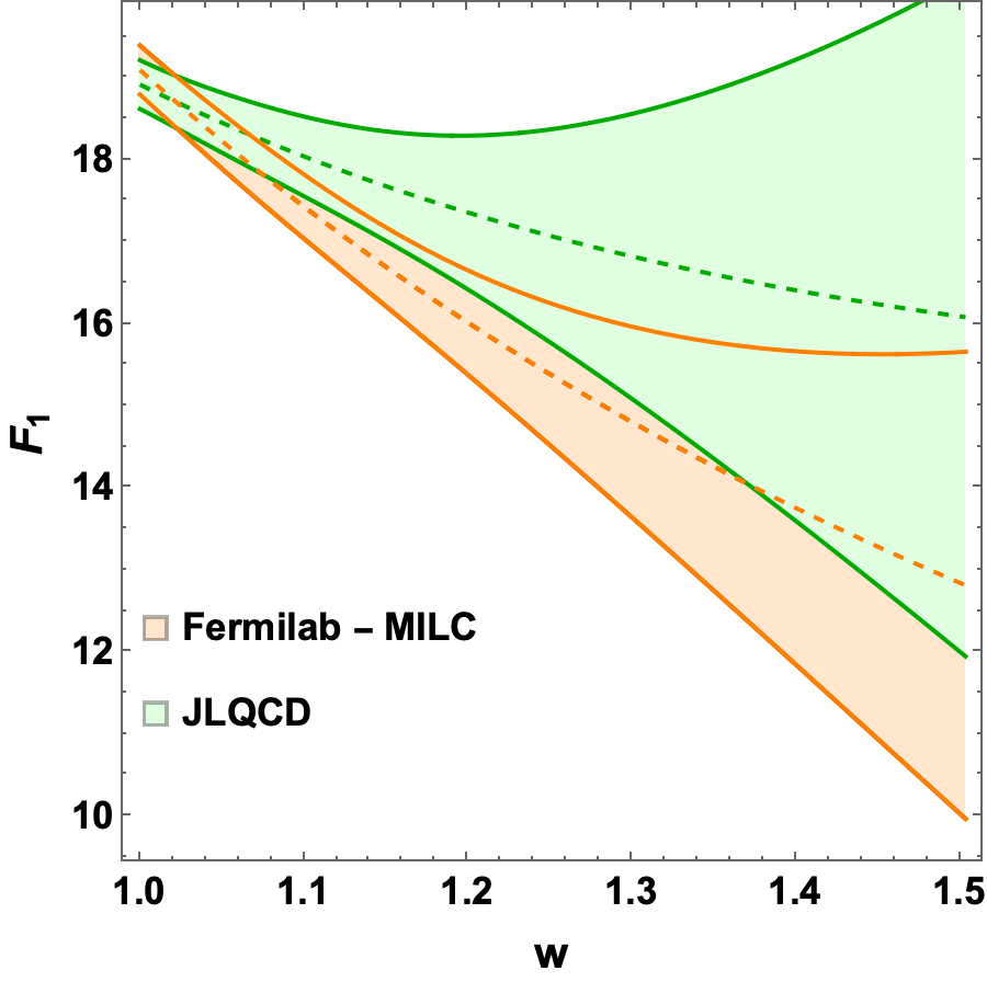
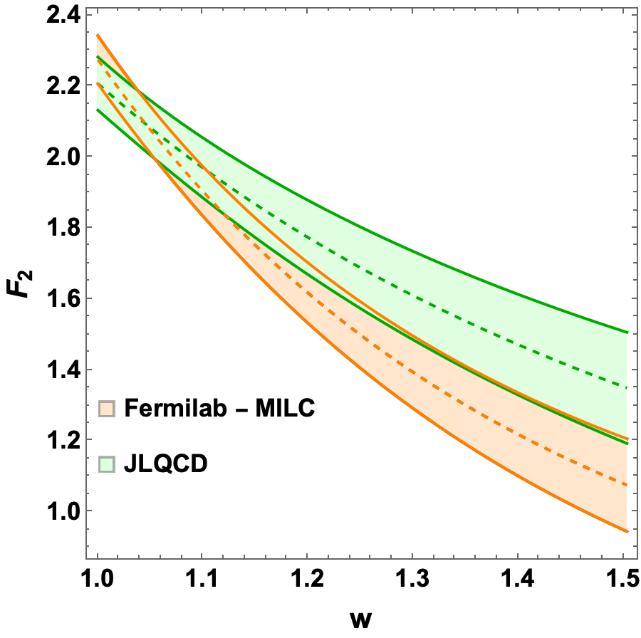
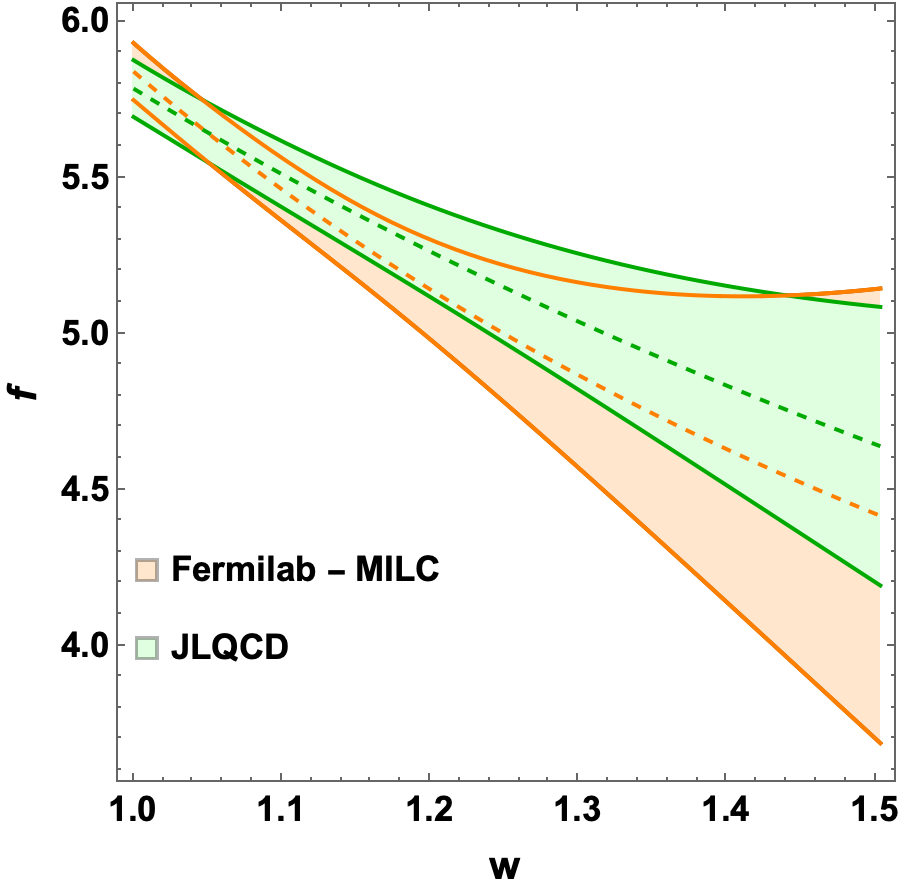
The lattice QCD can compute the values of the form factors in the low w𝑀w region. Fermilab-MILC (FM) and JLQCD collaborations give the values of the four form factors, F≑(f,g,β„±1,β„±2)𝐹𝑓𝑔subscriptβ„±1subscriptβ„±2F\equiv(f,g,\mathcal{F}_{1},\mathcal{F}_{2}), at these three points: wFM=(1.03.1.10,1.17)subscript𝑀FM1.03.1.101.17w_{\rm FM}=(1.03.1.10,1.17) for Fermilab-MILC collaboration and wJLQCD=(1.025.1.060,1.100)subscript𝑀JLQCD1.025.1.0601.100w_{\rm JLQCD}=(1.025.1.060,1.100) for JLQCDΒ 222Hereafter, we focus only on the results provided by these two collaboration as the result fromΒ [66] is given in terms of the HQET form factors and requires an extra transformation.. They also provides the 12Γ—12121212\times 12 covariance matrix for them. Using this lattice data, we fit the BGL parameters, aβ†’BGL=(anf,ang,anβ„±1,anβ„±2)subscriptβ†’π‘ŽBGLsubscriptsuperscriptπ‘Žπ‘“π‘›subscriptsuperscriptπ‘Žπ‘”π‘›subscriptsuperscriptπ‘Žsubscriptβ„±1𝑛subscriptsuperscriptπ‘Žsubscriptβ„±2𝑛\vec{a}_{\rm BGL}=(a^{f}_{n},a^{g}_{n},a^{\mathcal{F}_{1}}_{n},a^{\mathcal{F}_{2}}_{n}), given in Eq.Β (12). The Ο‡2superscriptπœ’2\chi^{2} can be symbolically written as

Ο‡latt2​(aβ†’BGL)=(Fβ†’BGL​(wlatt)βˆ’Fβ†’latt​(wlatt))​Vlattβˆ’1​(Fβ†’BGL​(wlatt)βˆ’Fβ†’latt​(wlatt))T,subscriptsuperscriptπœ’2lattsubscriptβ†’π‘ŽBGLsubscript→𝐹BGLsubscript𝑀lattsubscript→𝐹lattsubscript𝑀lattsuperscriptsubscript𝑉latt1superscriptsubscript→𝐹BGLsubscript𝑀lattsubscript→𝐹lattsubscript𝑀latt𝑇\chi^{2}_{\rm latt}(\vec{a}_{\rm BGL})=(\vec{F}_{\rm BGL}(w_{\rm latt})-\vec{F}_{\rm latt}(w_{\rm latt}))V_{\rm latt}^{-1}(\vec{F}_{\rm BGL}(w_{\rm latt})-\vec{F}_{\rm latt}(w_{\rm latt}))^{T}, (17)

where ”lattβ€œ is either FM or JLQCD. The Fβ†’latt​(wlatt)subscript→𝐹lattsubscript𝑀latt\vec{F}_{\rm latt}(w_{\rm latt}) are the form factors evaluated by the lattice and Vlattsubscript𝑉lattV_{\rm latt} is the covariance matrix mentioned above. The Fβ†’BGL​(wlatt)subscript→𝐹BGLsubscript𝑀latt\vec{F}_{\rm BGL}(w_{\rm latt}) are the form factor expanded in terms of the BGL parameters aβ†’BGLsubscriptβ†’π‘ŽBGL\vec{a}_{\rm BGL} and evaluated, using Eq.Β (12), at wlattsubscript𝑀lattw_{\rm latt}. We keep terms up to n=2𝑛2n=2 in the following. Using the two relations in Eqs.Β (15) and (16), we eliminate a0β„±1subscriptsuperscriptπ‘Žsubscriptβ„±10a^{\mathcal{F}_{1}}_{0} and a2β„±2subscriptsuperscriptπ‘Žsubscriptβ„±22a^{\mathcal{F}_{2}}_{2} and we fit 10 parameters. The fit results for JLQCD and Fermilab-MILC are given in TableΒ 4, in the second and third coumns, respectively.
Refer to caption Refer to caption
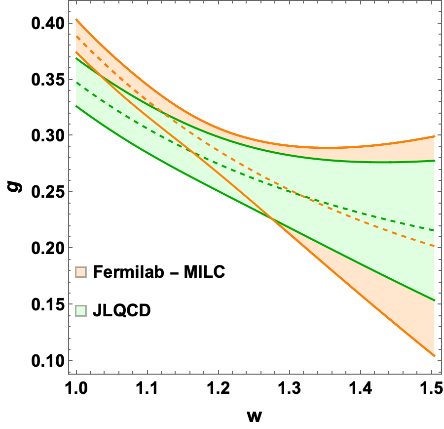
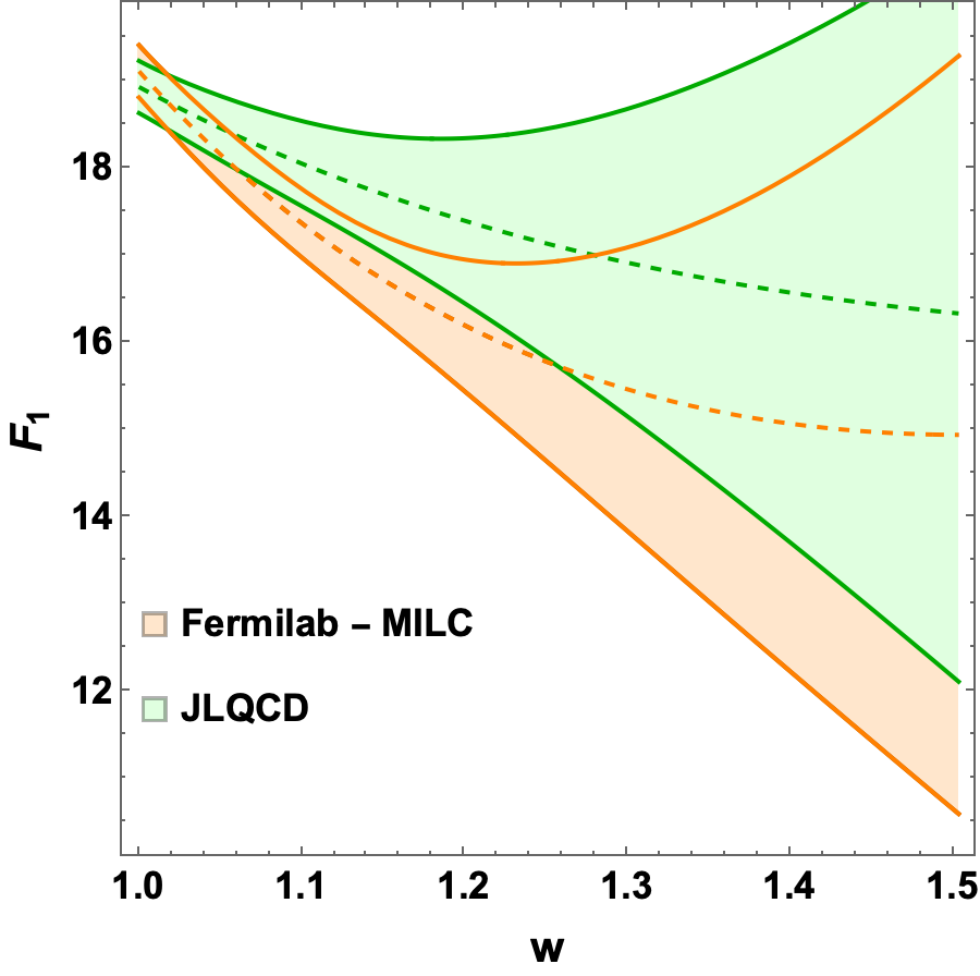
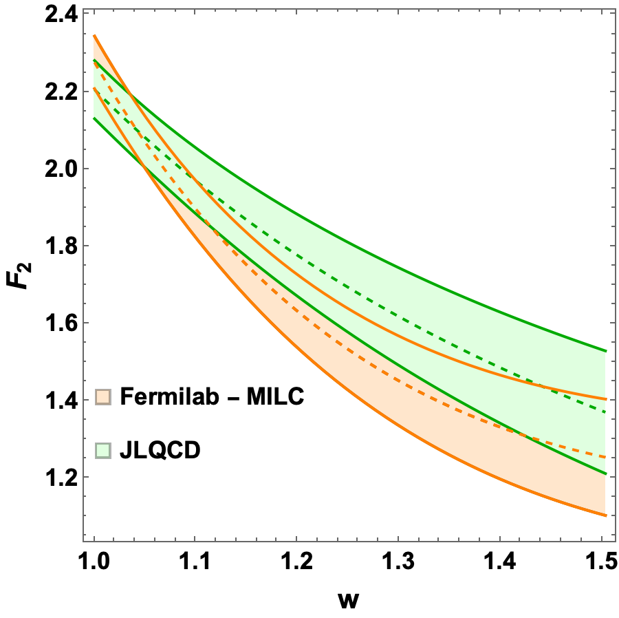
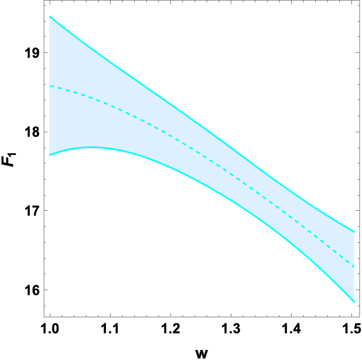
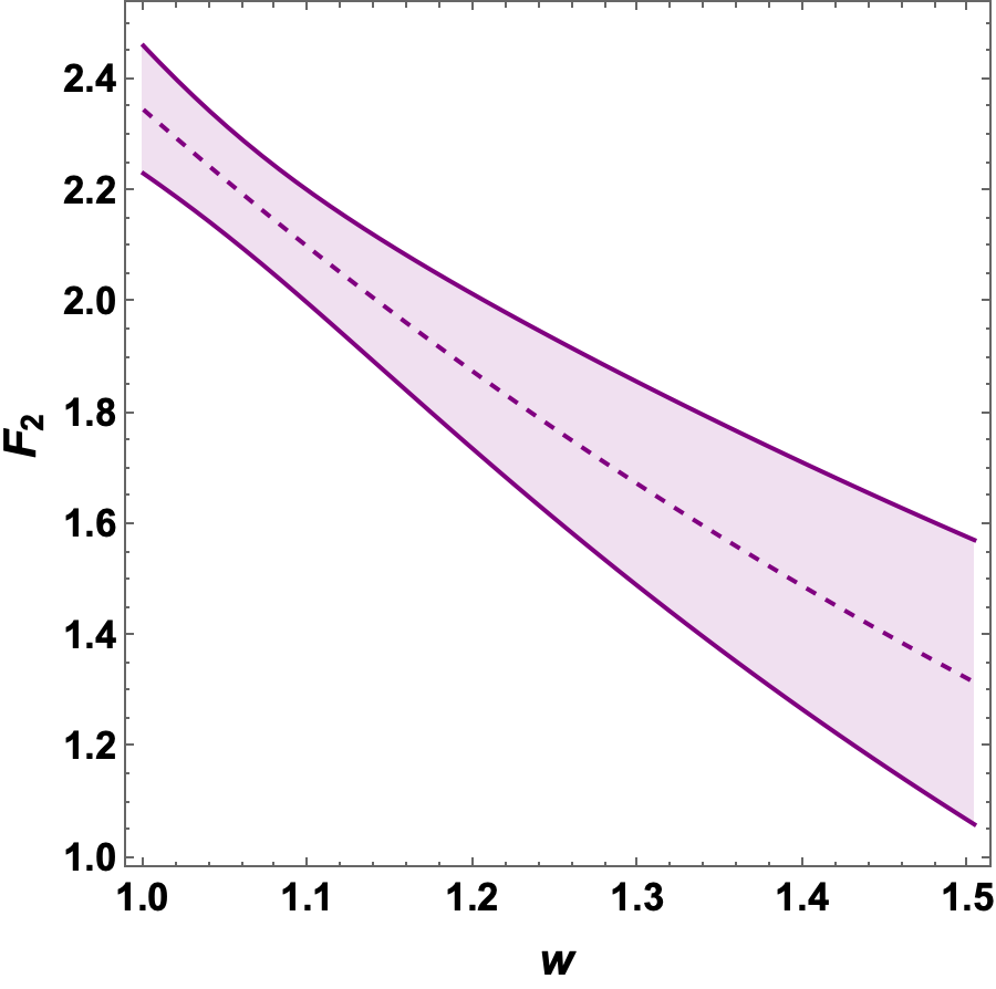
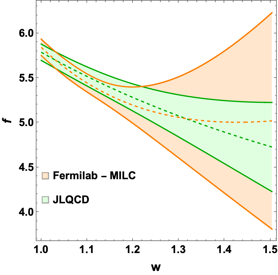
Figure 2: The extrapolated w𝑀w-dependence of the form factors using the BGL parameteristaion: the green and orange bounds are obtained by using the lattice QCD inputs at the low w𝑀w region by the JLQCD and the Fermilab-MILC collaborations, respectively. No unitarity condition is imposed in these plots.

Previously, the only lattice QCD result available was for β„±β„±\mathcal{F} at zero-recoil:

ℱ​(1)≑12​MB​MDβˆ—β€‹a0fP1+​(0)​ϕf​(0)β„±112subscript𝑀𝐡subscript𝑀superscript𝐷subscriptsuperscriptπ‘Žπ‘“0subscript𝑃superscript10subscriptitalic-ϕ𝑓0\mathcal{F}(1)\equiv\frac{1}{2\sqrt{M_{B}M_{D^{*}}}}\frac{a^{f}_{0}}{P_{1^{+}}(0)\phi_{f}(0)} (18)

with the value being ℱ​(1)=0.906Β±0.004Β±0.012β„±1plus-or-minus0.9060.0040.012\mathcal{F}(1)=0.906\pm 0.004\pm 0.012Β [71]. With the new lattice results, the fitted value of a0fsubscriptsuperscriptπ‘Žπ‘“0a^{f}_{0} above gives:

β„±JLQCD​(1)=0.887Β±0.014,β„±FM​(1)=0.896Β±0.014formulae-sequencesuperscriptβ„±JLQCD1plus-or-minus0.8870.014superscriptβ„±FM1plus-or-minus0.8960.014\mathcal{F}^{\rm JLQCD}(1)=0.887\pm 0.014,\quad\mathcal{F}^{\rm FM}(1)=0.896\pm 0.014

Using these values, we can extrapolate the form factors to higher value of w𝑀w. The extrapolated plots are shown in Fig.Β 2. As mentioned earlier, the expansion parameters have constraints coming from the unitarity, i.e. Eq.Β (14). One can impose these limit by adding some prior like

Ο‡unitarityβˆ’bound2=aBGL2subscriptsuperscriptπœ’2unitarityboundsuperscriptsubscriptπ‘ŽBGL2\chi^{2}_{\rm unitarity-bound}=a_{\rm BGL}^{2} (19)

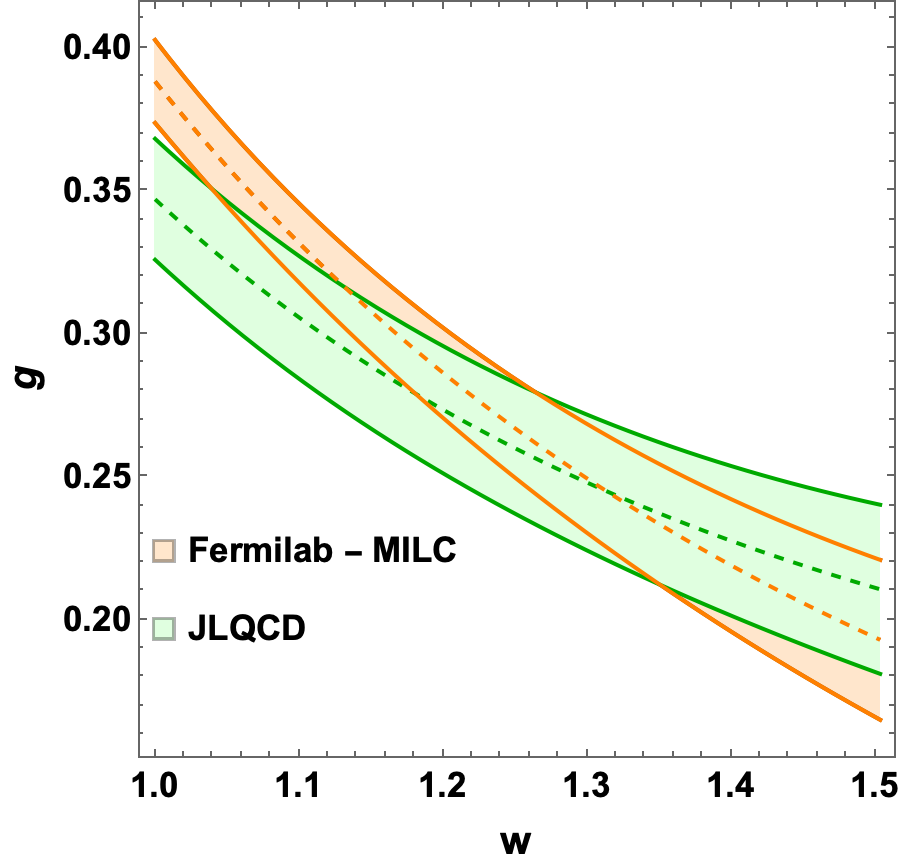
The results obtained with this prior are given in TableΒ 4 in the fourth and fifth column for JLQCD and Fermilab-MILC, respectively. The extrapolated plots are shown in Fig.Β 3. Even after taking into account the unitarity bound, the lattice QCD data itself does not constrain well the higher w𝑀w region. As we will see in the next section, the experimental data has a much better handle on this.
Refer to caption Refer to caption
Figure 3: The extrapolated w𝑀w-dependence of the form factors using the BGL parameteristaion: the green and orange bounds are obtained by using the lattice QCD inputs at the low w𝑀w region by the JLQCD and the Fermilab-MILC collaborations, respectively. The unitarity condition is imposed by using a prior given in Eq.Β (19).

5 The Belle binned results in the light of lattice data

The BaBar and Belle collaborations used their data and obtained the form factors along with the CKM matrix element Vc​bsubscript𝑉𝑐𝑏V_{cb} inΒ [61, 62, 63, 74, 75, 76]. They use the binned distribution of one of the four kinematical variables, w,cos⁑θl,cos⁑θV𝑀subscriptπœƒπ‘™subscriptπœƒπ‘‰w,\cos\theta_{l},\cos\theta_{V} or Ο‡πœ’\chi. It is a one dimensional distribution where the other 3 variables are integrated each time:

d​Γ​(w)=8​K9​π​{6​J1​s+3​J1​cβˆ’2​J2​sβˆ’J2​c}d​Γ​(cos⁑θV)=βˆ’4​K3​π​{βˆ’83​J1​s+(83​J1​sβˆ’4​J1​c)​cos2⁑θV}d​Γ​(cos⁑θℓ)=4​K3​π​{(43​J1​s+2​J1​c)+2​J6​s​cos⁑θℓ+(43​J1​sβˆ’2​J1​c)​cos2⁑θℓ}d​Γ​(Ο‡)=4​K9​{(163​J1​s+4​J1​c)+4​J3​cos⁑(2​χ)+4​J9​sin⁑(2​χ)}𝑑Γ𝑀absent8𝐾9πœ‹6subscript𝐽1𝑠3subscript𝐽1𝑐2subscript𝐽2𝑠subscript𝐽2𝑐𝑑Γsubscriptπœƒπ‘‰absent4𝐾3πœ‹83subscript𝐽1𝑠83subscript𝐽1𝑠4subscript𝐽1𝑐superscript2subscriptπœƒπ‘‰π‘‘Ξ“subscriptπœƒβ„“absent4𝐾3πœ‹43subscript𝐽1𝑠2subscript𝐽1𝑐2subscript𝐽6𝑠subscriptπœƒβ„“43subscript𝐽1𝑠2subscript𝐽1𝑐superscript2subscriptπœƒβ„“π‘‘Ξ“πœ’absent4𝐾9163subscript𝐽1𝑠4subscript𝐽1𝑐4subscript𝐽32πœ’4subscript𝐽92πœ’\displaystyle\begin{aligned} d\Gamma(w)&=\frac{8K}{9}\pi\Big{\{}6J_{1s}+3J_{1c}-2J_{2s}-J_{2c}\Big{\}}\\ d\Gamma(\cos\theta_{V})&=-\frac{4K}{3}\pi\Big{\{}{-\frac{8}{3}J_{1s}}+({\frac{8}{3}J_{1s}-4J_{1c}})\cos^{2}\theta_{V}\Big{\}}\\ d\Gamma(\cos\theta_{\ell})&=\frac{4K}{3}\pi\Big{\{}({\frac{4}{3}J_{1s}+2J_{1c}})+{2J_{6s}}\cos\theta_{\ell}+({\frac{4}{3}J_{1s}-2J_{1c}})\cos^{2}\theta_{\ell}\Big{\}}\\ d\Gamma(\chi)&=\frac{4K}{9}\Big{\{}({\frac{16}{3}J_{1s}+4J_{1c}})+{4J_{3}}\cos(2{\chi})+{4J_{9}}\sin(2{\chi})\Big{\}}\end{aligned} (20)

where K=3​MB​MDβˆ—24​(4​π)4​w2βˆ’1​(1βˆ’2​w​r+r2)​GF2​|Ξ·EW|2​|Vc​b|2​ℬ​(Dβˆ—β†’D​π)𝐾3subscript𝑀𝐡superscriptsubscript𝑀superscript𝐷24superscript4πœ‹4superscript𝑀2112π‘€π‘Ÿsuperscriptπ‘Ÿ2superscriptsubscript𝐺𝐹2superscriptsubscriptπœ‚EW2superscriptsubscript𝑉𝑐𝑏2ℬ→superscriptπ·π·πœ‹K=\frac{3M_{B}M_{D^{*}}^{2}}{4(4\pi)^{4}}\sqrt{w^{2}-1}(1-2\,w\,r+r^{2})\,G_{F}^{2}\,{\color[rgb]{0,0,0}|\eta_{\rm EW}|^{2}}\left|V_{cb}\right|^{2}\mathcal{B}(D^{*}\to D\pi). They divided each distribution into 10 bins and thus, the number of events for the total of 40 bins are published together with the detector response matrix and the selection efficiency, the systematic uncertainties and the 40Γ—40404040\times 40 statistical uncertainty correlation matrix. The correlation among the bins are obtained using the SM theoretical formula.

In this section, we first reproduce the result of BelleΒ [62], where the form factors as well as the |Vc​b|subscript𝑉𝑐𝑏|V_{cb}| are extracted from the data within the SM framework. As mentioned earlier, the |Vc​b|subscript𝑉𝑐𝑏|V_{cb}| is an overall factor and can not be extracted without an input of at least one form factor. In SectionΒ 5.1, we first obtain the tilde parameters, a~BGL≑aBGL​|Vc​b|​ηE​Wsubscript~π‘ŽBGLsubscriptπ‘ŽBGLsubscript𝑉𝑐𝑏subscriptπœ‚πΈπ‘Š\tilde{a}_{\rm BGL}\equiv a_{\rm BGL}|V_{cb}|\eta_{EW}, which is independent of the form factor. Then, in SectionΒ 5.2, we use the lattice results introduced in the SectionΒ 4, and fit the form factors and |Vc​b|subscript𝑉𝑐𝑏|V_{cb}| simultaneously. In SectionΒ 5.3, we extend our model from SM to the one including right-handed current, parameterised by CVRsubscript𝐢subscriptVRC_{\rm V_{R}} and perform the fit of form factor, |Vc​b|subscript𝑉𝑐𝑏|V_{cb}| and CVRsubscript𝐢subscriptVRC_{\rm V_{R}}. There is a caveat on the last analysis: the correlation of the Belle result is obtained based on the SM theory formula. Thus, the result of SectionΒ 5.3 remains as just a demonstration and we suggest the Belle collaboration to obtain the correlation including right-handed model to perform the fit.

5.1 Form factor determination with Belle data

In this section we obtain the tilde parameters from the Belle data published inΒ [62]. The Ο‡2superscriptπœ’2\chi^{2} to minimise can be written as

Ο‡Belle2​(a~β†’BGL)=βˆ‘i,j(Niobsβˆ’Niexp)​Ci​jβˆ’1​(Njobsβˆ’Njexp)subscriptsuperscriptπœ’2Bellesubscriptβ†’~π‘ŽBGLsubscript𝑖𝑗superscriptsubscript𝑁𝑖obssuperscriptsubscript𝑁𝑖expsubscriptsuperscript𝐢1𝑖𝑗superscriptsubscript𝑁𝑗obssuperscriptsubscript𝑁𝑗exp\displaystyle\chi^{2}_{\rm Belle}(\vec{\tilde{a}}_{\rm BGL})=\sum_{i,j}(N_{i}^{\rm obs}-N_{i}^{\rm exp})C^{-1}_{ij}(N_{j}^{\rm obs}-N_{j}^{\rm exp}) (21)

where Niobssuperscriptsubscript𝑁𝑖obsN_{i}^{\rm obs} is the observed number of events, Niexpsubscriptsuperscript𝑁exp𝑖N^{\rm exp}_{i} is the expected number of events and Ci​jsubscript𝐢𝑖𝑗C_{ij} is the covariance matrix. To avoid the problem with the highly correlated experimental uncertainties, we follow the procedure given inΒ [77] and perform a Toy Monte Carlo (MC): the MC samples are generated by using the Cholesky decomposition method for both statistical and systematic covariance matrices Cstat,systsubscript𝐢statsystC_{\rm stat,syst}

Nobs⁣′=Nobs+L​u,C=L​LTformulae-sequencesuperscript𝑁obsβ€²superscript𝑁obs𝐿𝑒𝐢𝐿superscript𝐿𝑇N^{{\rm obs}\prime}=N^{\rm obs}+Lu,\quad C=LL^{T} (22)

where u𝑒u is the random value taken from a Gaussian distribution of mean 0 and variance 1. We iterate the fit a few thousands times with this MC sample and average the result to obtain the best fit values for the parameters as well as the error matrix.

Form factor Value
a~0fsubscriptsuperscript~π‘Žπ‘“0\tilde{a}^{f}_{0} 0.000459​(9)​(20)0.0004599200.000459(9)(20)
a~1fsubscriptsuperscript~π‘Žπ‘“1\tilde{a}^{f}_{1} 0.0017​(13)​(13)0.001713130.0017(13)(13)
a~2fsubscriptsuperscript~π‘Žπ‘“2\tilde{a}^{f}_{2} βˆ’0.013​(43)​(32)0.0134332-0.013(43)(32)
a~0gsubscriptsuperscript~π‘Žπ‘”0\tilde{a}^{g}_{0} 0.0016​(6)​(5)0.0016650.0016(6)(5)
a~1gsubscriptsuperscript~π‘Žπ‘”1\tilde{a}^{g}_{1} βˆ’0.019​(24)​(21)0.0192421-0.019(24)(21)
a~2gsubscriptsuperscript~π‘Žπ‘”2\tilde{a}^{g}_{2} βˆ’0.02​(17)​(17)0.021717-0.02(17)(17)
a~1β„±1subscriptsuperscript~π‘Žsubscriptβ„±11\tilde{a}^{\mathcal{F}_{1}}_{1} βˆ’0.0003​(1)​(1)0.000311-0.0003(1)(1)
a~2β„±1subscriptsuperscript~π‘Žsubscriptβ„±12\tilde{a}^{\mathcal{F}_{1}}_{2} βˆ’0.0028​(19)​(16)0.00281916-0.0028(19)(16)
Table 5: The BGL parameters fitted by using the Belle data published in [62]. The tilde notation is defined as a~BGL≑aBGL​|Vc​b|​ηEWsubscript~π‘ŽBGLsubscriptπ‘ŽBGLsubscript𝑉𝑐𝑏subscriptπœ‚EW\tilde{a}_{\rm BGL}\equiv a_{\rm BGL}|V_{cb}|\eta_{\rm EW}. The first error is statistical and the second is systematic.
Refer to caption Refer to caption
Refer to caption
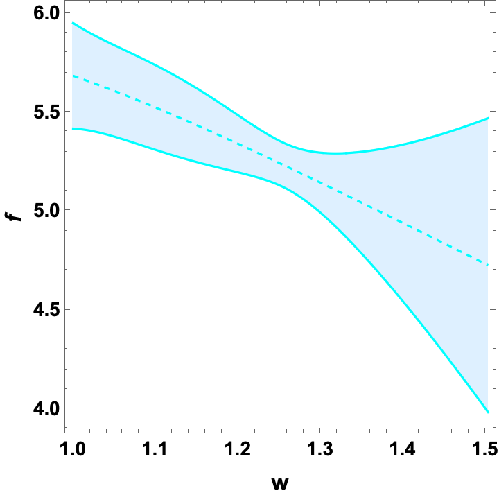
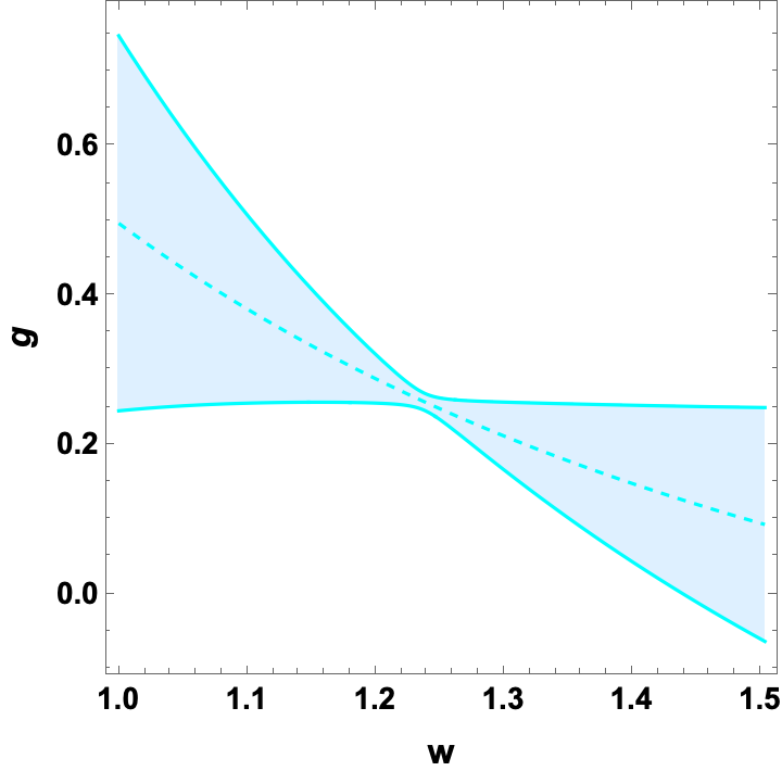
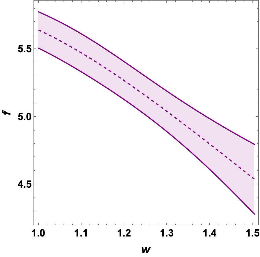
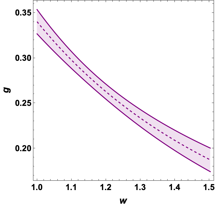
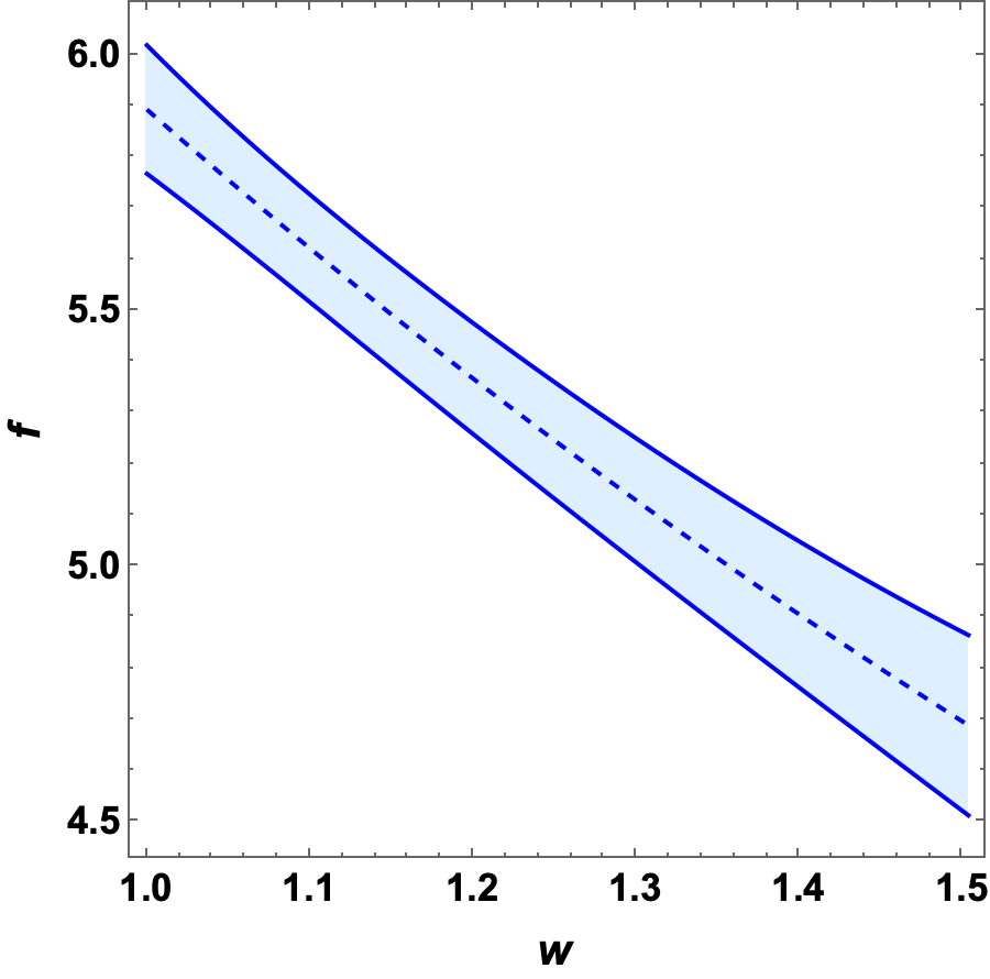
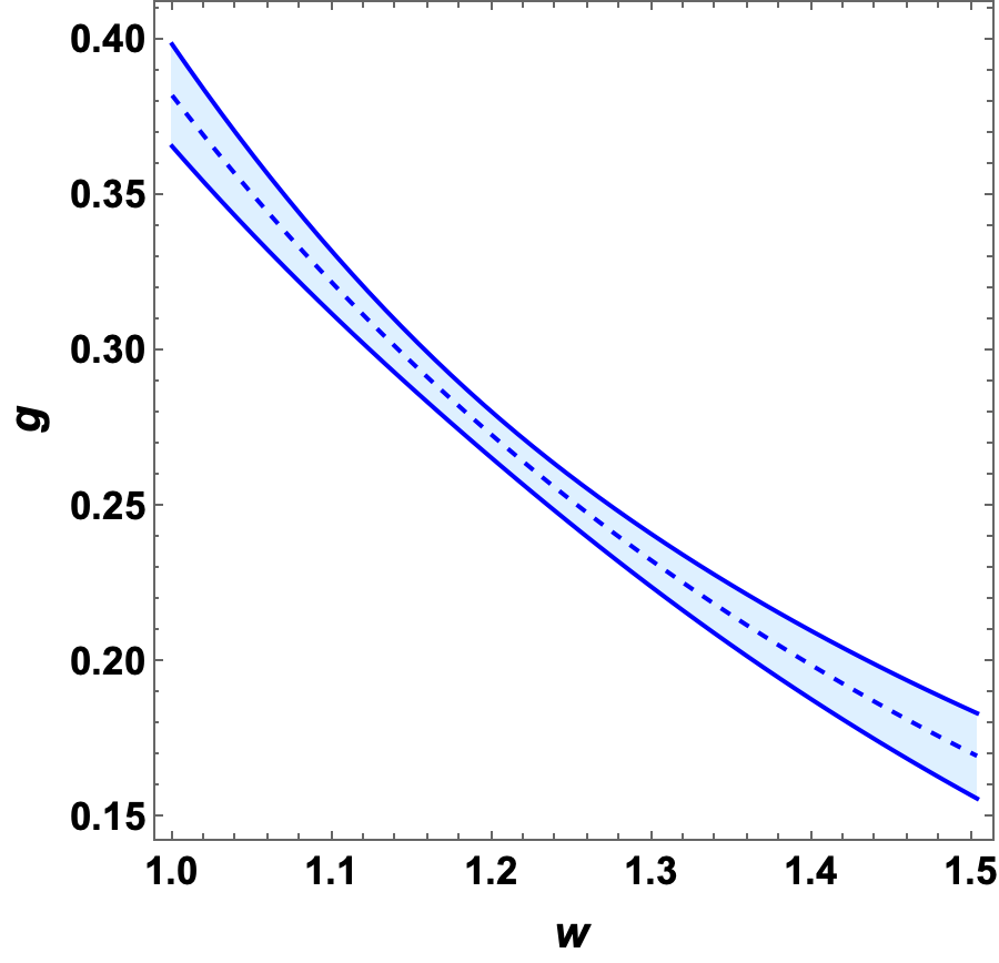
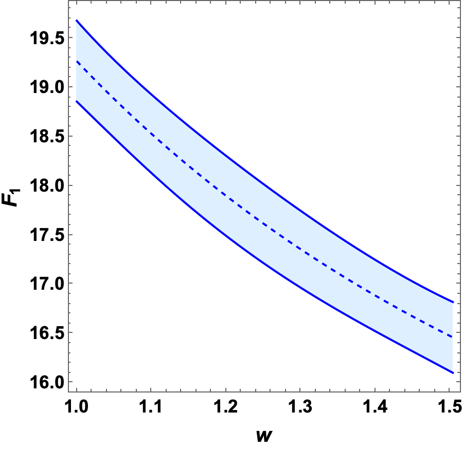
Figure 4: The w𝑀w-dependence of the form factors using the fitted BGL parameters with the Belle data Β [62]. Note that the originally obtained BGL parameters are in the tilde form, i.e. a~BGL≑aBGL​|Vc​b|​ηEWsubscript~π‘ŽBGLsubscriptπ‘ŽBGLsubscript𝑉𝑐𝑏subscriptπœ‚EW\tilde{a}_{\rm BGL}\equiv a_{\rm BGL}|V_{cb}|\eta_{\rm EW}. In this figure, we use a factor |Vc​b|​ηEW=0.039subscript𝑉𝑐𝑏subscriptπœ‚EW0.039|V_{cb}|\eta_{\rm EW}=0.039 to relate it to the BGL parameter, aBGLsubscriptπ‘ŽBGLa_{\rm BGL} so as to be able to compare to the w𝑀w-dependence of the form factors in the other figures.

The obtained results are given in TableΒ 4, where the first error is statistical and the second one is systematic. Since the distribution doesn’t depend on the β„±2subscriptβ„±2\mathcal{F}_{2}, we fit only eight parameters here. The result agrees qualitatively well with the results given inΒ [62]. Using this results, we may draw the f,g,F1𝑓𝑔subscript𝐹1f,g,F_{1} form factors in terms of w𝑀w. However, as the obtained result from the fit is a~BGLsubscript~π‘ŽBGL\tilde{a}_{\rm BGL}, we have to scale it by a factor |Vc​b|​ηEWsubscript𝑉𝑐𝑏subscriptπœ‚EW|V_{cb}|\eta_{\rm EW} to obtain aBGLsubscriptπ‘ŽBGL{a}_{\rm BGL}. Just for the sake of comparing the w𝑀w dependence with Fig.Β 2, we chose here a scaling factor as 0.039 and the result is given in Fig.Β 4.

5.2 SM fit of the Belle data with the new lattice data

Next, we will perform the fit including the new lattice data given in SectionΒ 4. The new Ο‡2superscriptπœ’2\chi^{2} to minimise is the sum of Eq.(17) and Eq.(21), i.e.

Ο‡Belle+latt2​(aβ†’BGL,|Vc​b|)=Ο‡Belle2​(aβ†’BGL,|Vc​b|)+Ο‡latt2​(aβ†’BGL)subscriptsuperscriptπœ’2Bellelattsubscriptβ†’π‘ŽBGLsubscript𝑉𝑐𝑏subscriptsuperscriptπœ’2Bellesubscriptβ†’π‘ŽBGLsubscript𝑉𝑐𝑏subscriptsuperscriptπœ’2lattsubscriptβ†’π‘ŽBGL\chi^{2}_{\rm Belle+latt}(\vec{a}_{\rm BGL},|V_{cb}|)=\chi^{2}_{\rm Belle}(\vec{a}_{\rm BGL},|V_{cb}|)+\chi^{2}_{\rm latt}(\vec{a}_{\rm BGL}) (23)

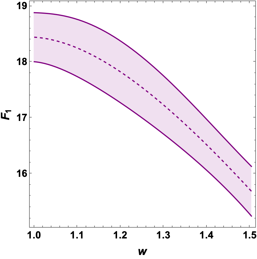
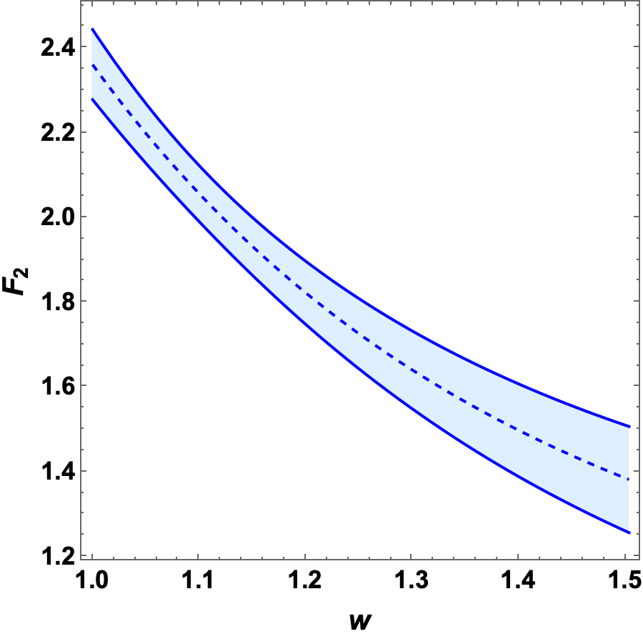
Now, we can determine both the form factor parameters aβ†’BGLsubscriptβ†’π‘ŽBGL\vec{a}_{\rm BGL} and |Vc​b|subscript𝑉𝑐𝑏|V_{cb}|. It is important to mention that in this case, we also have to generate the MC sample for the lattice data, by fluctuating them within their error, to perform the fit. The obtained fit results are given in TableΒ 6. Using the BGL parameters, we draw the w𝑀w dependence of the form factors, f,g,F1𝑓𝑔subscript𝐹1f,g,F_{1} and F2subscript𝐹2F_{2} (without prior) in Figs.Β 5 andΒ 6. We observe that the obtained bounds on f𝑓f, and especially on g𝑔g form factors becomes very narrow in whole region of w𝑀w, as compared to Figs.Β 2 and Β 3. This seems to come from the fact that the Belle data constrains these parameters in the middle range of w𝑀w as seen in Fig.Β 4. Together with the lattice data constraint in the lower w𝑀w region, these two form factors become well constrained in the whole range of w𝑀w.

Concerning |Vc​b|subscript𝑉𝑐𝑏|V_{cb}|, with the Ξ·EW=1.0066subscriptπœ‚EW1.0066\eta_{\rm EW}=1.0066, we find

|Vc​b|=0.0394Β±0.0011JLQCD|Vc​b|=0.0386Β±0.0009Fermilabβˆ’MILCsubscript𝑉𝑐𝑏plus-or-minus0.03940.0011JLQCDsubscript𝑉𝑐𝑏plus-or-minus0.03860.0009FermilabMILC\displaystyle\begin{aligned} |V_{cb}|=0.0394\pm 0.0011\quad\quad\quad&{\rm JLQCD}\\ |V_{cb}|=0.0386\pm 0.0009\quad\quad\quad&{\rm Fermilab-MILC}\end{aligned} (24)

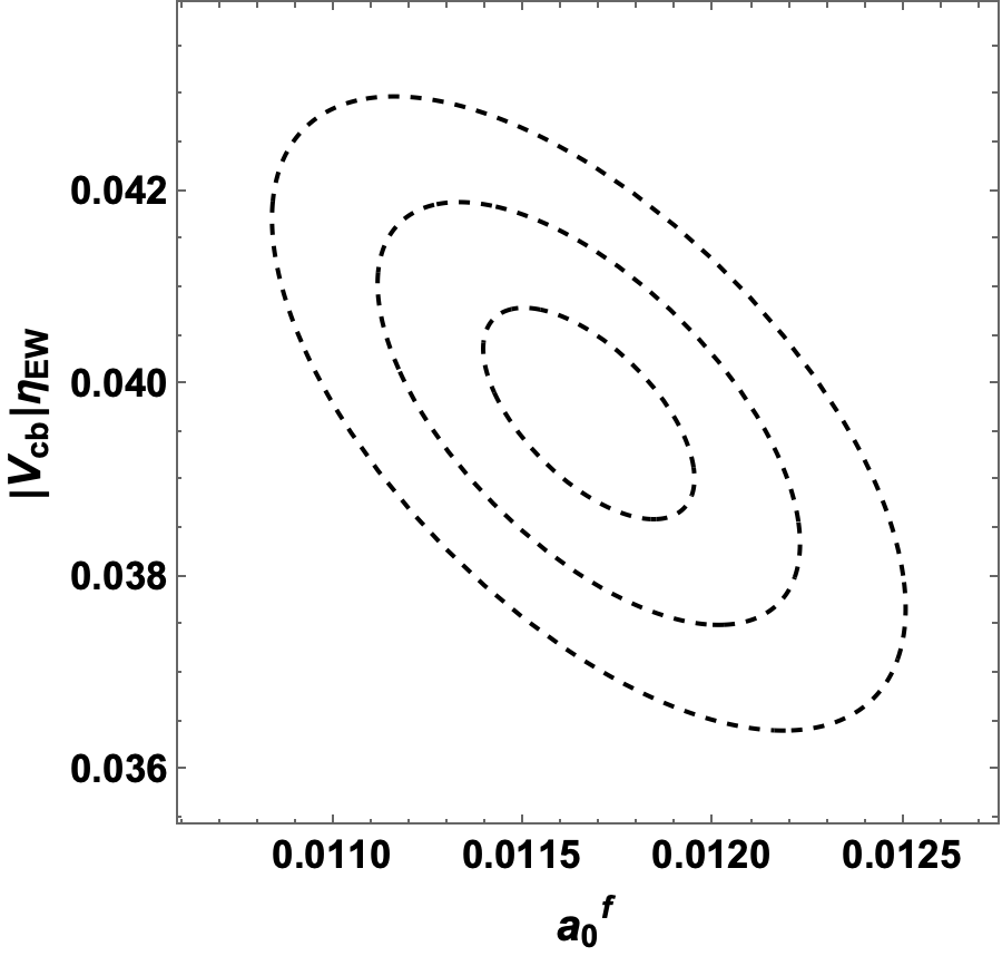
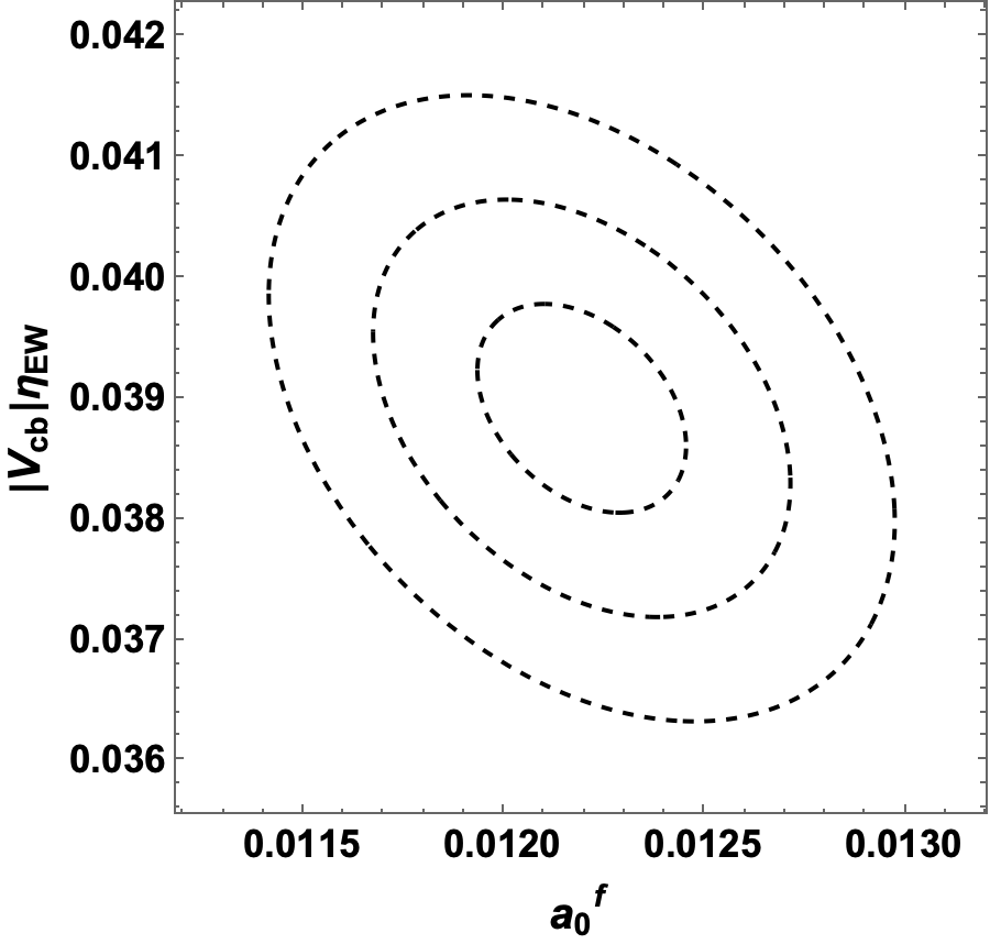
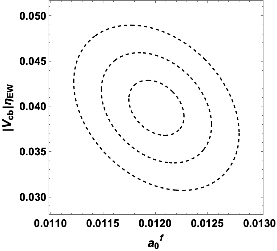
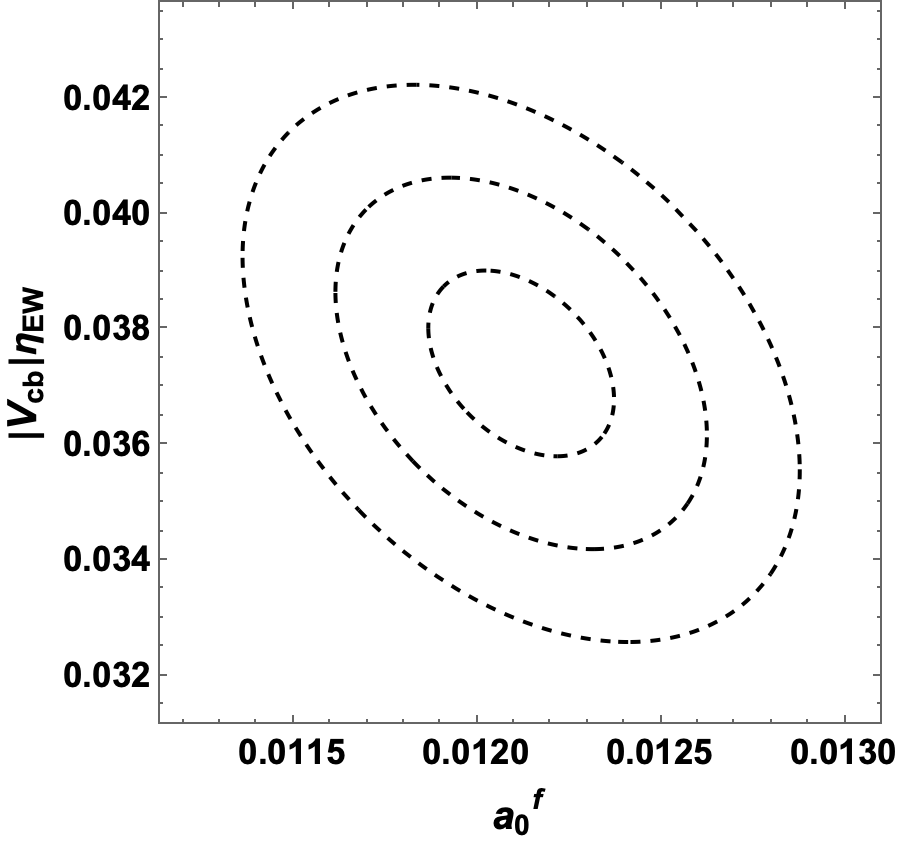
As expected, the |Vc​b|subscript𝑉𝑐𝑏|V_{cb}| is strongly correlated to the value of a0fsubscriptsuperscriptπ‘Žπ‘“0a^{f}_{0}, which is depicted in Fig.Β 7.

Fit parameters JLQCD Fermilab-MILC
a0fsubscriptsuperscriptπ‘Žπ‘“0a^{f}_{0} 0.01167​(23)​(16)0.0116723160.01167(23)(16) 0.01219​(17)​(19)0.0121917190.01219(17)(19)
a1fsubscriptsuperscriptπ‘Žπ‘“1a^{f}_{1} 0.0428​(70)​(69)0.042870690.0428(70)(69) 0.0233​(54)​(105)0.0233541050.0233(54)(105)
a2fsubscriptsuperscriptπ‘Žπ‘“2a^{f}_{2} βˆ’0.47​(20)​(26)0.472026-0.47(20)(26) βˆ’0.16​(12)​(17)0.161217-0.16(12)(17)
a0gsubscriptsuperscriptπ‘Žπ‘”0a^{g}_{0} 0.02876​(93)​(64)0.0287693640.02876(93)(64) 0.03229​(99)​(96)0.0322999960.03229(99)(96)
a1gsubscriptsuperscriptπ‘Žπ‘”1a^{g}_{1} βˆ’0.061​(33)​(25)0.0613325-0.061(33)(25) βˆ’0.166​(35)​(37)0.1663537-0.166(35)(37)
a2gsubscriptsuperscriptπ‘Žπ‘”2a^{g}_{2} βˆ’0.0165​(80)​(87)0.01658087-0.0165(80)(87) βˆ’0.03​(24)​(22)0.032422-0.03(24)(22)
a1F1subscriptsuperscriptπ‘Žsubscript𝐹11a^{F_{1}}_{1} 0.0089​(21)​(21)0.008921210.0089(21)(21) 0.0030​(13)​(18)0.003013180.0030(13)(18)
a2F1subscriptsuperscriptπ‘Žsubscript𝐹12a^{F_{1}}_{2} βˆ’0.109​(44)​(37)0.1094437-0.109(44)(37) 0.002​(26)​(25)0.00226250.002(26)(25)
a0F2subscriptsuperscriptπ‘Žsubscript𝐹20a^{F_{2}}_{0} 0.0515​(18)​(18)0.051518180.0515(18)(18) 0.0519​(12)​(13)0.051912130.0519(12)(13)
a1F2subscriptsuperscriptπ‘Žsubscript𝐹21a^{F_{2}}_{1} βˆ’0.03​(12)​(13)0.031213-0.03(12)(13) βˆ’0.175​(55)​(67)0.1755567-0.175(55)(67)
|Vc​b|​ηEWsubscript𝑉𝑐𝑏subscriptπœ‚EW|V_{cb}|\eta_{\rm EW} 0.03969​(86)​(67)0.0396986670.03969(86)(67) 0.03892​(52)​(69)0.0389252690.03892(52)(69)
Table 6: The BGL form factors and |Vc​b|​ηEWsubscript𝑉𝑐𝑏subscriptπœ‚EW|V_{cb}|\eta_{\rm EW} obtained by a simultaneous fit of the Belle dataΒ [62] and the lattice data by JLQCDΒ [65] (second column) and Fermilab-MILCΒ [64] (third column) collaborations. The first error is statistical and the second is systematic.
Refer to caption Refer to caption
Figure 5: The w𝑀w-dependence of the form factors using the fitted BGL parameters with the Belle data Β [62] and the JLQCD lattice dataΒ [65].
Refer to caption Refer to caption
Figure 6: The w𝑀w-dependence of the form factors using the fitted BGL parameters with the Belle data Β [62] and the Fermilab-MILC lattice dataΒ [64].
Β Β Β Β Β Β Β Β Β Β Β  Belle+JLQCD Β Β Β Β Β Β Β Β Β  Belle+Fermilab-MILC
Refer to caption Refer to caption
Figure 7: Correlation plots between a0fsubscriptsuperscriptπ‘Žπ‘“0a^{f}_{0} and |Vc​b|​ηEWsubscript𝑉𝑐𝑏subscriptπœ‚EW|V_{cb}|\eta_{\rm EW}, from combined fit of Belle dataΒ [62] and lattice data. The first plot is with JLQCD dataΒ [65] and the second plot is with Fermilab-MILC dataΒ [64].

5.3 Test of new physics by fitting the Belle and lattice data: example of right-handed model

In this section, we suggest the simultaneous fit of Belle and lattice data to test the new physics model with right-handed current as an example. Strictly speaking, we cannot use the currently available Belle data to perform this fit since its correlation assumes the SM as mentioned earlier. For this reason, our fit result is not completely reliable though, it may gives a useful instruction for the future analysis for Belle II.

With the right-handed contribution, the Jisubscript𝐽𝑖J_{i} functions which describe the differential decay rate in Eq.Β (9) include a new parameter CVRsubscript𝐢subscriptVRC_{\rm V_{R}} as given in TableΒ 1. In general CVRsubscript𝐢subscriptVRC_{\rm V_{R}} can be a complex number, but we assume it to be real parameter for simplicity in this section. Now the Ο‡2superscriptπœ’2\chi^{2} to fit is given as

Ο‡Belle+latt2​(aβ†’BGL,|Vc​b|,CVR)=Ο‡Belle2​(aβ†’BGL,|Vc​b|,CVR)+Ο‡latt2​(aβ†’BGL)subscriptsuperscriptπœ’2Bellelattsubscriptβ†’π‘ŽBGLsubscript𝑉𝑐𝑏subscript𝐢subscriptVRsubscriptsuperscriptπœ’2Bellesubscriptβ†’π‘ŽBGLsubscript𝑉𝑐𝑏subscript𝐢subscriptVRsubscriptsuperscriptπœ’2lattsubscriptβ†’π‘ŽBGL\displaystyle\chi^{2}_{\rm Belle+latt}(\vec{a}_{\rm BGL},|V_{cb}|,C_{\rm V_{R}})=\chi^{2}_{\rm Belle}(\vec{a}_{\rm BGL},|V_{cb}|,C_{\rm V_{R}})+\chi^{2}_{\rm latt}(\vec{a}_{\rm BGL}) (25)

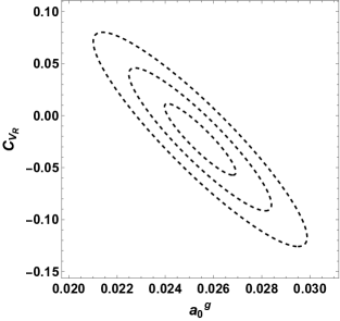
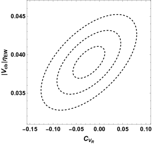
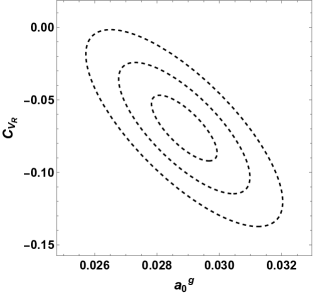
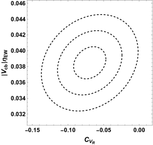
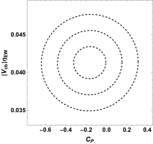
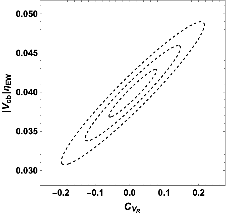
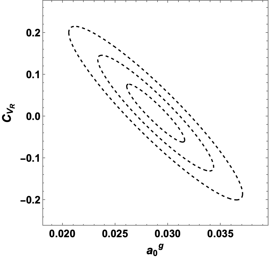
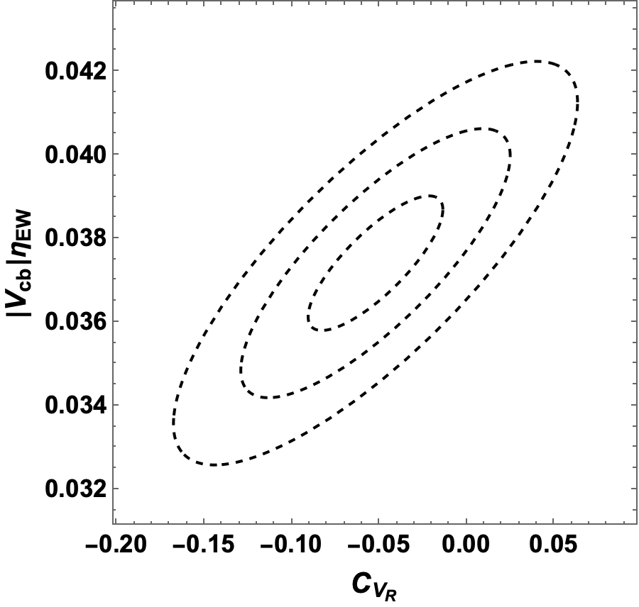
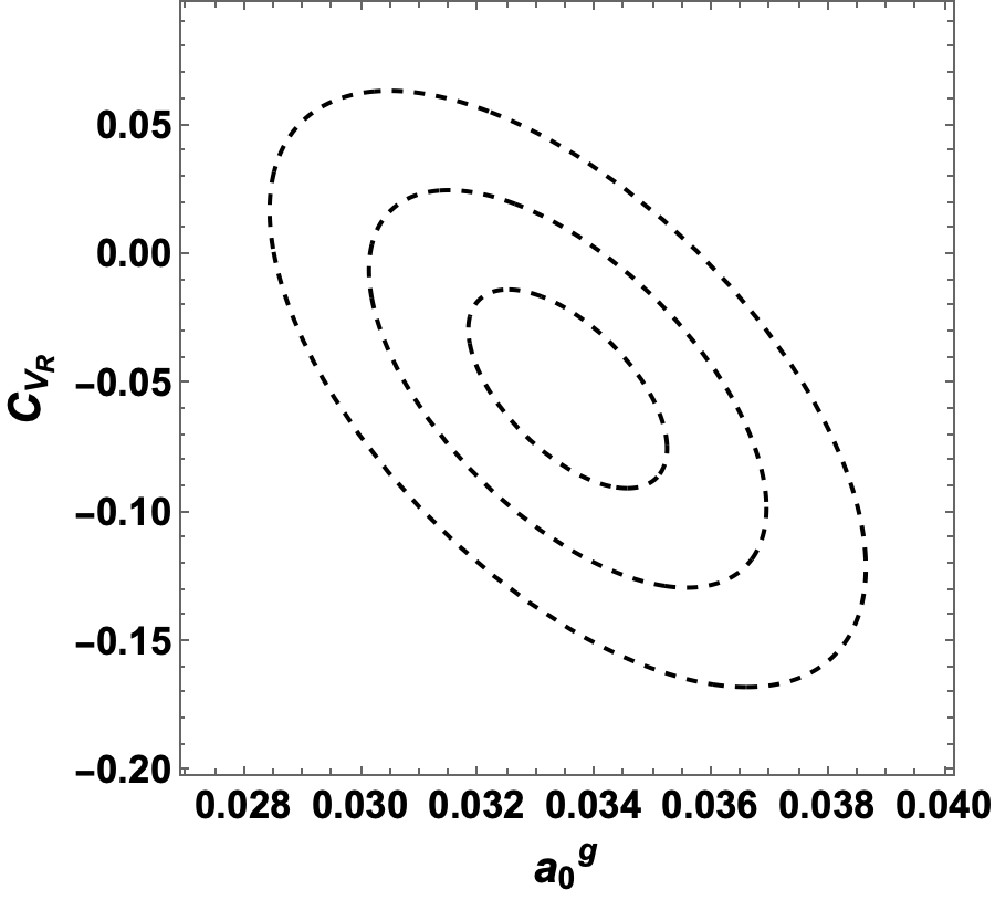
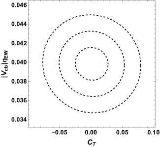
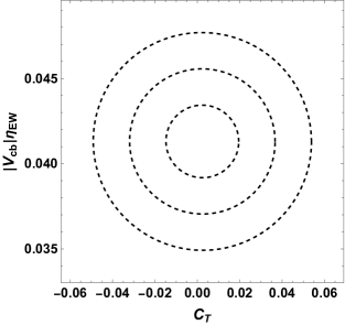
where the CVRsubscript𝐢subscriptVRC_{\rm V_{R}} is included in the Niexpsuperscriptsubscript𝑁𝑖expN_{i}^{\rm exp} in Ο‡Belle2subscriptsuperscriptπœ’2Belle\chi^{2}_{\rm Belle}. The obtained fit results are given in TableΒ 7. Here, we observe a significant difference between results with lattice inputs of JLQCD and Fermilab-MILC: CVRsubscript𝐢subscriptVRC_{\rm V_{R}} is zero consistent for JLQCD while the Fermilab-MILC shows a negative 5% shift. At the same time, the |Vc​b|subscript𝑉𝑐𝑏|V_{cb}| value decreases for the latter. Although it is not a significant effect, we attempt to understand better this phenomena. Looking at the error matrix, we find three large entries between a0fβˆ’|Vc​b|superscriptsubscriptπ‘Ž0𝑓subscript𝑉𝑐𝑏a_{0}^{f}-|V_{cb}|, a0gβˆ’CVRsuperscriptsubscriptπ‘Ž0𝑔subscript𝐢subscriptVRa_{0}^{g}-C_{\rm V_{R}} and |Vc​b|βˆ’CVRsubscript𝑉𝑐𝑏subscript𝐢subscriptVR|V_{cb}|-C_{\rm V_{R}}, which we show in Figs.Β 8 andΒ 9. Indeed, the central value of a0gsuperscriptsubscriptπ‘Ž0𝑔a_{0}^{g} for two lattice inputs disagree as seen in, for example, TableΒ 4, and that seems to be the reason for different CVRsubscript𝐢subscriptVRC_{\rm V_{R}} obtained in the fit. As the correlation between |Vc​b|subscript𝑉𝑐𝑏|V_{cb}| and CVRsubscript𝐢subscriptVRC_{\rm V_{R}} is positive, the negative CVRsubscript𝐢subscriptVRC_{\rm V_{R}} obtained for Fermilab-MILC lowers the value of |Vc​b|subscript𝑉𝑐𝑏|V_{cb}|. As mentioned in the introduction, the SM |Vc​b|subscript𝑉𝑐𝑏|V_{cb}| is expected to be higher than the nominal fit, this contradicts to the global picture. It is premature to give any conclusion, since i) we need the Belle collaboration to provide their correlation assuming right-handed current, ii) the two lattice collaboration do not agree on the vector form factor, namely a0gsuperscriptsubscriptπ‘Ž0𝑔a_{0}^{g}. Nevertheless, we urge both experimental and lattice collaborations to clarify these issues.

Fit parameters JLQCD Fermilab-MILC
a0fsubscriptsuperscriptπ‘Žπ‘“0a^{f}_{0} 0.01200​(20)​(18)0.0120020180.01200(20)(18) 0.01212​(19)​(17)0.0121219170.01212(19)(17)
a1fsubscriptsuperscriptπ‘Žπ‘“1a^{f}_{1} 0.0193​(34)​(69)0.019334690.0193(34)(69) 0.0193​(29)​(74)0.019329740.0193(29)(74)
a2fsubscriptsuperscriptπ‘Žπ‘“2a^{f}_{2} βˆ’0.036​(69)​(51)0.0366951-0.036(69)(51) βˆ’0.066​(25)​(26)0.0662526-0.066(25)(26)
a0gsubscriptsuperscriptπ‘Žπ‘”0a^{g}_{0} 0.0288​(19)​(20)0.028819200.0288(19)(20) 0.0335​(12)​(12)0.033512120.0335(12)(12)
a1gsubscriptsuperscriptπ‘Žπ‘”1a^{g}_{1} βˆ’0.070​(34)​(40)0.0703440-0.070(34)(40) βˆ’0.123​(46)​(49)0.1234649-0.123(46)(49)
a2gsubscriptsuperscriptπ‘Žπ‘”2a^{g}_{2} βˆ’0.0051​(71)​(59)0.00517159-0.0051(71)(59) βˆ’0.0060​(18)​(20)0.00601820-0.0060(18)(20)
a1F1subscriptsuperscriptπ‘Žsubscript𝐹11a^{F_{1}}_{1} 0.0051​(13)​(19)0.005113190.0051(13)(19) 0.0026​(11)​(15)0.002611150.0026(11)(15)
a2F1subscriptsuperscriptπ‘Žsubscript𝐹12a^{F_{1}}_{2} βˆ’0.049​(27)​(27)0.0492727-0.049(27)(27) 0.004​(23)​(22)0.00423220.004(23)(22)
a0F2subscriptsuperscriptπ‘Žsubscript𝐹20a^{F_{2}}_{0} 0.0481​(18)​(18)0.048118180.0481(18)(18) 0.0522​(12)​(12)0.052212120.0522(12)(12)
a1F2subscriptsuperscriptπ‘Žsubscript𝐹21a^{F_{2}}_{1} 0.030​(60)​(67)0.03060670.030(60)(67) βˆ’0.193​(50)​(52)0.1935052-0.193(50)(52)
CVRsubscript𝐢subscriptVRC_{\rm V_{R}} 0.008​(47)​(51)0.00847510.008(47)(51) βˆ’0.052​(27)​(28)0.0522728-0.052(27)(28)
|Vc​b|​ηEWsubscript𝑉𝑐𝑏subscriptπœ‚EW|V_{cb}|\eta_{\rm EW} 0.0399​(21)​(22)0.039921220.0399(21)(22) 0.0374​(11)​(12)0.037411120.0374(11)(12)
Table 7: The BGL form factors, CVRsubscript𝐢subscriptVRC_{\rm V_{R}} and |Vc​b|​ηEWsubscript𝑉𝑐𝑏subscriptπœ‚EW|V_{cb}|\eta_{\rm EW} obtained by a simultaneous fit of the Belle dataΒ [62] and the lattice data by JLQCDΒ [65] (second column) and Fermilab-MILCΒ [64] (third column) collaborations. The first error is statistical and the second is systematic.
Refer to caption Refer to caption
Refer to caption
Figure 8: Correlation plots between a0fsubscriptsuperscriptπ‘Žπ‘“0a^{f}_{0}, |Vc​b|​ηEWsubscript𝑉𝑐𝑏subscriptπœ‚EW|V_{cb}|\eta_{\rm EW} and CVRsubscript𝐢subscriptVRC_{\rm V_{R}}, from combined fit of Belle dataΒ [62] and JLQCD lattice dataΒ [65]. CVRsubscript𝐢subscript𝑉𝑅C_{V_{R}} is assumed to be real.
Refer to caption Refer to caption
Refer to caption
Figure 9: Correlation plots between a0fsubscriptsuperscriptπ‘Žπ‘“0a^{f}_{0}, a0gsubscriptsuperscriptπ‘Žπ‘”0a^{g}_{0}, |Vc​b|​ηEWsubscript𝑉𝑐𝑏subscriptπœ‚EW|V_{cb}|\eta_{\rm EW} and CVRsubscript𝐢subscriptVRC_{\rm V_{R}}, from combined fit of Belle dataΒ [62] and Fermilab-MILC lattice dataΒ [64]. CVRsubscript𝐢subscriptVRC_{\rm V_{R}} is assumed to be real.

6 Unbinned angular analysis of Bβ†’Dβˆ—β€‹β„“β€‹Ξ½β„“β†’π΅superscript𝐷ℓsubscriptπœˆβ„“{B}\to D^{*}\ell{\nu}_{\ell}\;

In this section, following the method introduced inΒ [67], we investigate the sensitivity of the new physics in the unbinned method. The Belle analysis is limited to the binned analysis as of today, while once higher statistics will be available, a possibility of the unbinned analysis will open. The unbinned analysis, with full kinematical information, unlike the binned method which uses only integrated one dimension information, should provide a more detailed information. In this section, we investigate the unbinned method to explore what new information we can obtain comparing to the binned method which is studied in the previous section.

As unbinned data is not available from Belle, we synthesise the data first: we use all the fitted parameters by Belle experiment inΒ [62] (form factors and Vc​bsubscript𝑉𝑐𝑏V_{cb}) as truth values, and reproduce the differential decay rate of Bβ†’Dβˆ—β€‹β„“β€‹Ξ½β„“β†’π΅superscript𝐷ℓsubscriptπœˆβ„“{B}\to D^{*}\ell{\nu}_{\ell}\;decay. Then, to compensate for the limited statistics, we first separate the data in w𝑀w bins of 10 equal intervals. Then, for each w𝑀w bin, we investigate the fully unbinned distribution of the 3 angles (cos⁑θv,cos⁑θℓ,Ο‡subscriptπœƒπ‘£subscriptπœƒβ„“πœ’\cos\theta_{v},\cos\theta_{\ell},\chi). This is the same strategy applied for the Pi(β€²)superscriptsubscript𝑃𝑖′P_{i}^{(\prime)} measurements at LHCb inΒ [78].

Comparing to our study inΒ [67], we have three new inputs for this work; i) we use new lattice data introduced in SectionΒ 4, ii) the new physics model includes not only right-handed current but also psudoscalar and tensor terms, iii) we include the branching ratio to the fit. The point iii) is important in order to determine the new physics parameters (i.e. CVR,P,Tsubscript𝐢subscriptVRPTC_{\rm V_{R},P,T}) and Vc​bsubscript𝑉𝑐𝑏V_{cb} simultaneously. In our previous work, we attempted to use the number of signal of Bβ†’Dβˆ—β€‹β„“β€‹Ξ½β„“β†’π΅superscript𝐷ℓsubscriptπœˆβ„“{B}\to D^{*}\ell{\nu}_{\ell}\;process for this purpose, but to compare its theoretical predictions to the experimental value, it requires experimental efficiency, which was not so easy to obtain. Using the branching ratio provides a much simpler solution.

6.1 Unbinned maximum likelihood method

Let us now illustrate how to perform the unbinned fit with maximum likelihood method. We start by obtaining the normalised Probability Density Function (PDF) in terms of the 11 independent angular observables Jisubscript𝐽𝑖J_{i}. For this, we first give the expression of decay rate integrated over all the angles

d​Γd​w=3​MB​MDβˆ—24​(4​π)2​GF2​|Vc​b|2​|Ξ·EW|2​ℬ​(Dβˆ—β†’D​π)​8​π9​(6​J1​sβ€²+3​J1​cβ€²βˆ’2​J2​sβ€²βˆ’J2​cβ€²)𝑑Γ𝑑𝑀3subscript𝑀𝐡superscriptsubscript𝑀superscript𝐷24superscript4πœ‹2superscriptsubscript𝐺𝐹2superscriptsubscript𝑉𝑐𝑏2superscriptsubscriptπœ‚EW2ℬ→superscriptπ·π·πœ‹8πœ‹96subscriptsuperscript𝐽′1𝑠3subscriptsuperscript𝐽′1𝑐2subscriptsuperscript𝐽′2𝑠subscriptsuperscript𝐽′2𝑐\frac{d\Gamma}{dw}=\frac{3M_{B}M_{D^{*}}^{2}}{4(4\pi)^{2}}G_{F}^{2}|V_{cb}|^{2}|\eta_{\rm EW}|^{2}\mathcal{B}(D^{*}\rightarrow D\pi)\frac{8\pi}{9}\left(6J^{\prime}_{1s}+3J^{\prime}_{1c}-2J^{\prime}_{2s}-J^{\prime}_{2c}\right) (26)

where Ji′≑Ji​w2βˆ’1​(1βˆ’2​w​r+r2)subscriptsuperscript𝐽′𝑖subscript𝐽𝑖superscript𝑀2112π‘€π‘Ÿsuperscriptπ‘Ÿ2J^{\prime}_{i}\equiv J_{i}\sqrt{w^{2}-1}(1-2wr+r^{2}). Then, we integrate over each w𝑀w-bin and define the integrated decay rate as

βŸ¨Ξ“βŸ©wβˆ’binsubscriptdelimited-βŸ¨βŸ©Ξ“π‘€bin\displaystyle\langle\Gamma\rangle_{w-\rm bin} =3​MB​MDβˆ—24​(4​π)2​GF2​|Vc​b|2​|Ξ·EW|2​ℬ​(Dβˆ—β†’D​π)absent3subscript𝑀𝐡superscriptsubscript𝑀superscript𝐷24superscript4πœ‹2superscriptsubscript𝐺𝐹2superscriptsubscript𝑉𝑐𝑏2superscriptsubscriptπœ‚EW2ℬ→superscriptπ·π·πœ‹\displaystyle=\frac{3M_{B}M_{D^{*}}^{2}}{4(4\pi)^{2}}G_{F}^{2}|V_{cb}|^{2}|\eta_{\rm EW}|^{2}\mathcal{B}(D^{*}\rightarrow D\pi) (27)
Γ—8​π9​(6β€‹βŸ¨J1​sβ€²βŸ©wβˆ’bin+3β€‹βŸ¨J1​cβ€²βŸ©wβˆ’binβˆ’2β€‹βŸ¨J2​sβ€²βŸ©wβˆ’binβˆ’βŸ¨J2​cβ€²βŸ©wβˆ’bin)absent8πœ‹96subscriptdelimited-⟨⟩subscriptsuperscript𝐽′1𝑠𝑀bin3subscriptdelimited-⟨⟩subscriptsuperscript𝐽′1𝑐𝑀bin2subscriptdelimited-⟨⟩subscriptsuperscript𝐽′2𝑠𝑀binsubscriptdelimited-⟨⟩subscriptsuperscript𝐽′2𝑐𝑀bin\displaystyle\times\frac{8\pi}{9}\left(6\langle J^{\prime}_{1s}\rangle_{w-\rm bin}+3\langle J^{\prime}_{1c}\rangle_{w-\rm bin}-2\langle J^{\prime}_{2s}\rangle_{w-\rm bin}-\langle J^{\prime}_{2c}\rangle_{w-\rm bin}\right)

where

⟨Ji⟩wβˆ’binβ‰‘βˆ«wβˆ’binJi​𝑑wsubscriptdelimited-⟨⟩subscript𝐽𝑖𝑀binsubscript𝑀binsubscript𝐽𝑖differential-d𝑀\langle J_{i}\rangle_{w-{\rm bin}}\equiv\int_{w-{\rm bin}}J_{i}dw

Hereafter, the index ”w𝑀w-bin” is implicit. The normalised PDF for each w𝑀w-bin now can be written by the new normalised angular coefficients ⟨gβŸ©β†’=⟨giβŸ©β†’delimited-βŸ¨βŸ©π‘”delimited-⟨⟩subscript𝑔𝑖\vec{\langle g\rangle}=\langle g_{i}\rangle as

f^⟨gβ†’βŸ©β€‹(cos⁑θV,cos⁑θℓ,Ο‡)=98​π{16(1βˆ’3⟨g1​c⟩+2⟨g2​s⟩+⟨g2​c⟩)sin2ΞΈV+⟨g1​c⟩cos2ΞΈV+(⟨g2​sβŸ©β€‹sin2⁑θV+⟨g2​cβŸ©β€‹cos2⁑θV)​cos⁑2​θl+⟨g3βŸ©β€‹sin2⁑θV​sin2⁑θl​cos⁑2​χl+⟨g4βŸ©β€‹sin⁑2​θV​sin⁑2​θl​cos⁑χl+⟨g5βŸ©β€‹sin⁑2​θV​sin⁑θl​cos⁑χl+(⟨g6​sβŸ©β€‹sin2⁑θV+⟨g6​cβŸ©β€‹cos2⁑θV)​cos⁑θl+⟨g7βŸ©β€‹sin⁑2​θV​sin⁑θl​sin⁑χl+⟨g8βŸ©β€‹sin⁑2​θV​sin⁑2​θl​sin⁑χl+⟨g9⟩sin2ΞΈVsin2ΞΈlsin2Ο‡l}\displaystyle\begin{aligned} \hat{f}_{\langle\vec{g}\rangle}(\cos\theta_{V},\cos\theta_{\ell},\chi)&=\frac{9}{8\pi}\Big{\{}\frac{1}{6}(1-3\langle g_{1c}\rangle+2\langle g_{2s}\rangle+\langle g_{2c}\rangle)\sin^{2}\theta_{V}+\langle g_{1c}\rangle\cos^{2}\theta_{V}\\ &+(\langle g_{2s}\rangle\sin^{2}\theta_{V}+\langle g_{2c}\rangle\cos^{2}\theta_{V})\cos 2\theta_{l}\\ &+\langle g_{3}\rangle\sin^{2}\theta_{V}\sin^{2}\theta_{l}\cos 2\chi_{l}+\langle g_{4}\rangle\sin 2\theta_{V}\sin 2\theta_{l}\cos\chi_{l}\\ &+\langle g_{5}\rangle\sin 2\theta_{V}\sin\theta_{l}\cos\chi_{l}+(\langle g_{6s}\rangle\sin^{2}\theta_{V}+\langle g_{6c}\rangle\cos^{2}\theta_{V})\cos\theta_{l}\\ &+\langle g_{7}\rangle\sin 2\theta_{V}\sin\theta_{l}\sin\chi_{l}+\langle g_{8}\rangle\sin 2\theta_{V}\sin 2\theta_{l}\sin\chi_{l}\\ &+\langle g_{9}\rangle\sin^{2}\theta_{V}\sin^{2}\theta_{l}\sin 2\chi_{l}\Big{\}}\end{aligned} (28)

where

⟨giβŸ©β‰‘βŸ¨Jiβ€²βŸ©6β€‹βŸ¨J1​sβ€²βŸ©+3β€‹βŸ¨J1​cβ€²βŸ©βˆ’2β€‹βŸ¨J2​sβ€²βŸ©βˆ’βŸ¨J2​cβ€²βŸ©delimited-⟨⟩subscript𝑔𝑖delimited-⟨⟩subscriptsuperscript𝐽′𝑖6delimited-⟨⟩subscriptsuperscript𝐽′1𝑠3delimited-⟨⟩subscriptsuperscript𝐽′1𝑐2delimited-⟨⟩subscriptsuperscript𝐽′2𝑠delimited-⟨⟩subscriptsuperscript𝐽′2𝑐\langle g_{i}\rangle\equiv\frac{\langle J^{\prime}_{i}\rangle}{6\langle J^{\prime}_{1s}\rangle+3\langle J^{\prime}_{1c}\rangle-2\langle J^{\prime}_{2s}\rangle-\langle J^{\prime}_{2c}\rangle} (29)

Then, we can write the log-likelihood to determine the angular coefficients ⟨gβ†’βŸ©delimited-βŸ¨βŸ©β†’π‘”\langle\vec{g}\rangle from the data:

ℒ​(⟨gβ†’βŸ©)=βˆ‘i=1Nl​n​f^⟨gβ†’βŸ©β€‹(ei)β„’delimited-βŸ¨βŸ©β†’π‘”superscriptsubscript𝑖1𝑁𝑙𝑛subscript^𝑓delimited-βŸ¨βŸ©β†’π‘”subscript𝑒𝑖\mathcal{L}(\langle\vec{g}\rangle)=\sum_{i=1}^{N}ln\hat{f}_{\langle\vec{g}\rangle}(e_{i}) (30)

where eisubscript𝑒𝑖e_{i} are the experimental events in (cos⁑θV,cos⁑θℓ,Ο‡subscriptπœƒπ‘‰subscriptπœƒβ„“πœ’\cos\theta_{V},\cos\theta_{\ell},\chi) and N𝑁N are the number of events for each w𝑀w-bin. The best fit value for ⟨gi⟩delimited-⟨⟩subscript𝑔𝑖\langle g_{i}\rangle is obtained by maximising the likelihood

βˆ‚β„’βˆ‚βŸ¨gi⟩|⟨gi⟩=⟨gi⟩fit=0evaluated-atβ„’delimited-⟨⟩subscript𝑔𝑖delimited-⟨⟩subscript𝑔𝑖subscriptdelimited-⟨⟩subscript𝑔𝑖fit0\left.\frac{\partial\mathcal{L}}{\partial\langle g_{i}\rangle}\right|_{\langle g_{i}\rangle=\langle g_{i}\rangle_{\rm fit}}=0 (31)

The inverse of the covariance matrix can be obtained by

Vi​jβˆ’1=βˆ‚2β„’βˆ‚βŸ¨giβŸ©β€‹βˆ‚βŸ¨gj⟩|⟨gi⟩=⟨gi⟩fitsubscriptsuperscript𝑉1𝑖𝑗evaluated-atsuperscript2β„’delimited-⟨⟩subscript𝑔𝑖delimited-⟨⟩subscript𝑔𝑗delimited-⟨⟩subscript𝑔𝑖subscriptdelimited-⟨⟩subscript𝑔𝑖fitV^{-1}_{ij}=\left.\frac{\partial^{2}\mathcal{L}}{\partial\langle g_{i}\rangle\partial\langle g_{j}\rangle}\right|_{\langle g_{i}\rangle=\langle g_{i}\rangle_{\rm fit}} (32)

Just to be clear, Vi​jsubscript𝑉𝑖𝑗V_{ij} is the 11Γ—11111111\times 11 matrix for each w𝑀w-bin (so we need 10 of these matrix if we have 10 bins in w𝑀w).

6.2 Fitting the theory parameters with the pseudo-data together with the lattice inputs

In this work, instead of performing a Toy Monte Carlo with generated events, we obtain directly ⟨gi⟩fitsubscriptdelimited-⟨⟩subscript𝑔𝑖fit\langle g_{i}\rangle_{\rm fit} as well as Vi​jsubscript𝑉𝑖𝑗V_{ij} from the normalised PDF f^⟨gβ†’βŸ©subscript^𝑓delimited-βŸ¨βŸ©β†’π‘”\hat{f}_{\langle\vec{g}\rangle} with truth inputs (i.e. the fitted form factors and Vc​bsubscript𝑉𝑐𝑏V_{cb} inΒ [62] as mentioned earlier). The detailed procedure is given in the AppendixΒ B.

Now, we can fit the theory parameters to the ’experimentally’ obtained angular coefficients and their correlations by using the following Ο‡2superscriptπœ’2\chi^{2}:

Ο‡angle2​(aβ†’BGL,CNP)=subscriptsuperscriptπœ’2anglesubscriptβ†’π‘ŽBGLsubscript𝐢NPabsent\displaystyle\chi^{2}_{\rm angle}(\vec{a}_{\rm BGL},C_{\rm NP})= (33)
βˆ‘wβˆ’bin=110[Nwβˆ’bin​V^i​jβˆ’1​(⟨giexpβŸ©βˆ’βŸ¨gith​(aβ†’BGL,CNP)⟩)​(⟨gjexpβŸ©βˆ’βŸ¨gjth​(aβ†’BGL,CNP)⟩)]wβˆ’binsuperscriptsubscript𝑀bin110subscriptdelimited-[]subscript𝑁𝑀binsubscriptsuperscript^𝑉1𝑖𝑗delimited-⟨⟩superscriptsubscript𝑔𝑖expdelimited-⟨⟩superscriptsubscript𝑔𝑖thsubscriptβ†’π‘ŽBGLsubscript𝐢NPdelimited-⟨⟩superscriptsubscript𝑔𝑗expdelimited-⟨⟩superscriptsubscript𝑔𝑗thsubscriptβ†’π‘ŽBGLsubscript𝐢NP𝑀bin\displaystyle\sum_{w-{\rm bin}=1}^{10}\left[N_{w-{\rm bin}}\hat{V}^{-1}_{ij}\left(\langle g_{i}^{\rm exp}\rangle-\langle g_{i}^{\rm th}(\vec{a}_{\rm BGL},C_{\rm NP})\rangle\right)\left(\langle g_{j}^{\rm exp}\rangle-\langle g_{j}^{\rm th}(\vec{a}_{\rm BGL},C_{\rm NP})\rangle\right)\right]_{w-{\rm bin}}

where V^^𝑉\hat{V} is the scaled covariance matrix, Nwβˆ’binsubscript𝑁𝑀binN_{w-{\rm bin}} are the number of events in the w𝑀w-bin and ⟨giexp⟩delimited-⟨⟩superscriptsubscript𝑔𝑖exp\langle g_{i}^{\rm exp}\rangle is the best fit value of the angular coefficients (see AppendixΒ B for details) while ⟨gith​(aβ†’BGL,CNP)⟩delimited-⟨⟩superscriptsubscript𝑔𝑖thsubscriptβ†’π‘ŽBGLsubscript𝐢NP\langle g_{i}^{\rm th}(\vec{a}_{\rm BGL},C_{\rm NP})\rangle are the theoretical expressions, which depend on the form factors and NP Wilson coefficients. We assume about the same amount of the signal events as inΒ [62]. Note that as Ο‡angle2subscriptsuperscriptπœ’2angle\chi^{2}_{\rm angle} term is made from the normalised angular coefficients, the overall constants such as Vc​bsubscript𝑉𝑐𝑏V_{cb} gets cancelled.

In order to constrain from the total number of events, we use the world average of the branching ratio, as mentioned earlier:

ℬexp​(Bβ†’Dβˆ—β€‹β„“β€‹Ξ½)=0.0495Β±0.0011superscriptℬexp→𝐡superscriptπ·β„“πœˆplus-or-minus0.04950.0011\mathcal{B}^{\rm exp}(B\to D^{*}\ell\nu)=0.0495\pm 0.0011

Then, the Ο‡2superscriptπœ’2\chi^{2} from the branching ratio measurement can be written as,

χℬ2​(aβ†’BGL,Vc​b,CNP)=(ℬth​(aβ†’BGL,Vc​b,CNP)βˆ’0.04950.0011)2subscriptsuperscriptπœ’2ℬsubscriptβ†’π‘ŽBGLsubscript𝑉𝑐𝑏subscript𝐢NPsuperscriptsuperscriptℬthsubscriptβ†’π‘ŽBGLsubscript𝑉𝑐𝑏subscript𝐢NP0.04950.00112\chi^{2}_{\mathcal{B}}(\vec{a}_{\rm BGL},V_{cb},C_{\rm NP})=\left(\frac{\mathcal{B}^{\rm th}(\vec{a}_{\rm BGL},V_{cb},C_{\rm NP})-0.0495}{0.0011}\right)^{2} (34)

where ℬth​(aβ†’BGL,Vc​b,CNP)superscriptℬthsubscriptβ†’π‘ŽBGLsubscript𝑉𝑐𝑏subscript𝐢NP\mathcal{B}^{\rm th}(\vec{a}_{\rm BGL},V_{cb},C_{\rm NP}) is the theoretical prediction of the branching ratio including new physics contribution.

Finally adding the lattice constraint, the total Ο‡2superscriptπœ’2\chi^{2} to fit is

Ο‡unbinned2​(aβ†’BGL,Vc​b,CNP)=Ο‡angle2​(aβ†’BGL,CNP)+Ο‡latt2​(aβ†’BGL)+χℬ2​(aβ†’BGL,Vc​b,CNP)subscriptsuperscriptπœ’2unbinnedsubscriptβ†’π‘ŽBGLsubscript𝑉𝑐𝑏subscript𝐢NPsubscriptsuperscriptπœ’2anglesubscriptβ†’π‘ŽBGLsubscript𝐢NPsubscriptsuperscriptπœ’2lattsubscriptβ†’π‘ŽBGLsubscriptsuperscriptπœ’2ℬsubscriptβ†’π‘ŽBGLsubscript𝑉𝑐𝑏subscript𝐢NP\displaystyle\chi^{2}_{\rm unbinned}(\vec{a}_{\rm BGL},V_{cb},C_{\rm NP})=\chi^{2}_{\rm angle}(\vec{a}_{\rm BGL},C_{\rm NP})+\chi^{2}_{\rm latt}(\vec{a}_{\rm BGL})+\chi^{2}_{\mathcal{B}}(\vec{a}_{\rm BGL},V_{cb},C_{\rm NP}) (35)

In the following, we show the fit results. We assume single non-zero new physics coupling at a time (i.e. CVRβ‰ 0,CPβ‰ 0formulae-sequencesubscript𝐢subscriptVR0subscript𝐢P0C_{\rm V_{R}}\neq 0,C_{\rm P}\neq 0 or CTβ‰ 0subscript𝐢T0C_{\rm T}\neq 0 and also assume that they are real number.

6.2.1 Right-handed model: CVRβ‰ 0subscript𝐢subscriptVR0C_{\rm V_{R}}\neq 0

The fitted result is given in Table 8. Let us first compare this unbinned analysis result with the binned one given in Table 7. As our pseudodata does not have systematic error, we can compare only the statistical one (i.e. the first parenthesis in Table  7). As expected, the statistical errors are better for the unbinned analysis though, hardly a factor of 2 for CVRsubscript𝐢subscriptVRC_{\rm V_{R}}. Figs. 10 and 11 show the correlations, which are also very similar to the binned study in Figs. 8 and Fig. 9. The CVRsubscript𝐢subscriptVRC_{\rm V_{R}} is more significantly different from zero in this case.

Fit parameters JLQCD Fermilab-MILC
a0fsubscriptsuperscriptπ‘Žπ‘“0a^{f}_{0} 0.01294​(20)0.01294200.01294(20) 0.01327​(20)0.01327200.01327(20)
a1fsubscriptsuperscriptπ‘Žπ‘“1a^{f}_{1} 0.018​(11)0.018110.018(11) βˆ’0.005​(13)0.00513-0.005(13)
a2fsubscriptsuperscriptπ‘Žπ‘“2a^{f}_{2} βˆ’0.21​(53)0.2153-0.21(53) βˆ’0.28​(61)0.2861-0.28(61)
a0gsubscriptsuperscriptπ‘Žπ‘”0a^{g}_{0} 0.0255​(15)0.0255150.0255(15) 0.0289​(11)0.0289110.0289(11)
a1gsubscriptsuperscriptπ‘Žπ‘”1a^{g}_{1} βˆ’0.045​(35)0.04535-0.045(35) βˆ’0.130​(49)0.13049-0.130(49)
a2gsubscriptsuperscriptπ‘Žπ‘”2a^{g}_{2} 0.4​(11)0.4110.4(11) 1.0​(14)1.0141.0(14)
a1β„±1subscriptsuperscriptπ‘Žsubscriptβ„±11a^{\mathcal{F}_{1}}_{1} 0.0061​(22)0.0061220.0061(22) βˆ’0.0001​(23)0.000123-0.0001(23)
a2β„±1subscriptsuperscriptπ‘Žsubscriptβ„±12a^{\mathcal{F}_{1}}_{2} βˆ’0.095​(94)0.09594-0.095(94) βˆ’0.05​(10)0.0510-0.05(10)
a0β„±2subscriptsuperscriptπ‘Žsubscriptβ„±20a^{\mathcal{F}_{2}}_{0} 0.0483​(14)0.0483140.0483(14) 0.0537​(13)0.0537130.0537(13)
a1β„±2subscriptsuperscriptπ‘Žsubscriptβ„±21a^{\mathcal{F}_{2}}_{1} βˆ’0.004​(50)0.00450-0.004(50) βˆ’0.276​(62)0.27662-0.276(62)
CVRsubscript𝐢subscriptVRC_{\rm V_{R}} βˆ’0.023​(34)0.02334-0.023(34) βˆ’0.070​(23)0.07023-0.070(23)
|Vc​b|​ηEWsubscript𝑉𝑐𝑏subscriptπœ‚EW|V_{cb}|\eta_{\rm EW} 0.0390​(21)0.0390210.0390(21) 0.0385​(20)0.0385200.0385(20)
Table 8: The BGL form factors, CVRsubscript𝐢subscriptVRC_{\rm V_{R}} and |Vc​b|​ηEWsubscript𝑉𝑐𝑏subscriptπœ‚EW|V_{cb}|\eta_{\rm EW} obtained by a simultaneous fit of the pseudo-data and the lattice data by JLQCDΒ [65] (second column) and Fermilab-MILCΒ [64] (third column) collaborations. The errors are statistical only.
Refer to caption Refer to caption
Figure 10: Correlation plots between a0gsubscriptsuperscriptπ‘Žπ‘”0a^{g}_{0}, |Vc​b|​ηEWsubscript𝑉𝑐𝑏subscriptπœ‚EW|V_{cb}|\eta_{\rm EW} and CVRsubscript𝐢subscriptVRC_{\rm V_{R}}, from combined fit of the pseudo-data and JLQCD lattice dataΒ [65]. CVRsubscript𝐢subscriptVRC_{\rm V_{R}} is assumed to be real.
Refer to caption Refer to caption
Figure 11: Correlation plots between a0gsubscriptsuperscriptπ‘Žπ‘”0a^{g}_{0}, |Vc​b|​ηEWsubscript𝑉𝑐𝑏subscriptπœ‚EW|V_{cb}|\eta_{\rm EW} and CVRsubscript𝐢subscriptVRC_{\rm V_{R}}, from combined fit of the pseudo-data and Fermilab-MILC lattice dataΒ [64] CVRsubscript𝐢subscriptVRC_{\rm V_{R}} is assumed to be real.

6.2.2 Pseudoscalar model: CPβ‰ 0subscript𝐢P0C_{\rm P}\neq 0

As we can see in the TablesΒ 1 andΒ 2, the CPsubscript𝐢PC_{\rm P} parameter enters only to the angular observable J1​csubscript𝐽1𝑐J_{1c} in squared form, |CP|2superscriptsubscript𝐢P2|C_{\rm P}|^{2}. There is no interference with the SM term i.e. CVLsubscript𝐢subscriptVLC_{\rm V_{L}}, as such terms are proportional to the lepton mass, which is neglected. As a result the sensitivity to this parameter is quite poor. The fitted result is given in TableΒ 9 where we find that |CP|subscript𝐢P|C_{\rm P}| is constrained only at 20-30% precision. As mentioned earlier, the psuedoscalar form factor is obtained by relating it to the axial vector form factor. This could potentially induce an error from the uncertainties of charm and quark masses. However, we find that this error is negligible here: we tested this by inflating the errors in the quark masses by order of 1 GeV. The results on |CP|subscript𝐢P|C_{\rm P}| with JLQCD and Fermilab-MILC inputs are slightly different. As shown in Figs.Β 12 andΒ 13, there is a small correlation between CPsubscript𝐢PC_{\rm P} and a1β„±1superscriptsubscriptπ‘Ž1subscriptβ„±1a_{1}^{\mathcal{F}_{1}} whose values are different for these two inputs and this might be the reason of this difference. Also shown in Figs.Β 12 andΒ 13, the correlation between |CP|subscript𝐢P|C_{\rm P}| and |Vc​b|subscript𝑉𝑐𝑏|V_{cb}| is very small. Thus, a shift in |CP|subscript𝐢P|C_{\rm P}| would not influence the value of Vc​bsubscript𝑉𝑐𝑏V_{cb} as seen in the the case of CVRβ‰ 0subscript𝐢subscriptVR0C_{\rm V_{R}}\neq 0.

Fit parameters JLQCD Fermilab-MILC
a0fsubscriptsuperscriptπ‘Žπ‘“0a^{f}_{0} 0.01294​(20)0.01294200.01294(20) 0.01336​(20)0.01336200.01336(20)
a1fsubscriptsuperscriptπ‘Žπ‘“1a^{f}_{1} 0.018​(11)0.018110.018(11) βˆ’0.003​(13)0.00313-0.003(13)
a2fsubscriptsuperscriptπ‘Žπ‘“2a^{f}_{2} βˆ’0.20​(53)0.2053-0.20(53) βˆ’0.47​(61)0.4761-0.47(61)
a0gsubscriptsuperscriptπ‘Žπ‘”0a^{g}_{0} 0.02456​(60)0.02456600.02456(60) 0.02626​(70)0.02626700.02626(70)
a1gsubscriptsuperscriptπ‘Žπ‘”1a^{g}_{1} βˆ’0.057​(29)0.05729-0.057(29) βˆ’0.154​(45)0.15445-0.154(45)
a2gsubscriptsuperscriptπ‘Žπ‘”2a^{g}_{2} 0.6​(11)0.6110.6(11) 0.9​(12)0.9120.9(12)
a1β„±1subscriptsuperscriptπ‘Žsubscriptβ„±11a^{\mathcal{F}_{1}}_{1} 0.0062​(22)0.0062220.0062(22) βˆ’0.0003​(23)0.000323-0.0003(23)
a2β„±1subscriptsuperscriptπ‘Žsubscriptβ„±12a^{\mathcal{F}_{1}}_{2} βˆ’0.095​(94)0.09594-0.095(94) βˆ’0.08​(10)0.0810-0.08(10)
a0β„±2subscriptsuperscriptπ‘Žsubscriptβ„±20a^{\mathcal{F}_{2}}_{0} 0.0484​(14)0.0484140.0484(14) 0.0530​(13)0.0530130.0530(13)
a1β„±2subscriptsuperscriptπ‘Žsubscriptβ„±21a^{\mathcal{F}_{2}}_{1} βˆ’0.002​(50)0.00250-0.002(50) βˆ’0.271​(61)0.27161-0.271(61)
|CP|subscript𝐢P|C_{\rm P}| βˆ’0.08​(33)0.0833-0.08(33) βˆ’0.17​(16)0.1716-0.17(16)
|Vc​b|​ηEWsubscript𝑉𝑐𝑏subscriptπœ‚EW|V_{cb}|\eta_{\rm EW} 0.0398​(17)0.0398170.0398(17) 0.0413​(21)0.0413210.0413(21)
Table 9: The BGL form factors, |CP|subscript𝐢P|C_{\rm P}| and |Vc​b|​ηEWsubscript𝑉𝑐𝑏subscriptπœ‚EW|V_{cb}|\eta_{\rm EW} obtained by a simultaneous fit of the pseudo-data and the lattice data by JLQCDΒ [65] (second column) and Fermilab-MILCΒ [64] (third column) collaborations. The errors are statistical only.
Refer to caption Refer to caption
Figure 12: Correlation plots between a1β„±1subscriptsuperscriptπ‘Žsubscriptβ„±11a^{\mathcal{F}_{1}}_{1}, |Vc​b|​ηEWsubscript𝑉𝑐𝑏subscriptπœ‚EW|V_{cb}|\eta_{\rm EW} and |CP|subscript𝐢P|C_{\rm P}|, from combined fit of the pseudo-data and JLQCD lattice dataΒ [65].
Refer to caption Refer to caption
Figure 13: Correlation plots between a1β„±1subscriptsuperscriptπ‘Žsubscriptβ„±11a^{\mathcal{F}_{1}}_{1}, |Vc​b|​ηEWsubscript𝑉𝑐𝑏subscriptπœ‚EW|V_{cb}|\eta_{\rm EW} and |CP|subscript𝐢P|C_{\rm P}|, from combined fit of the pseudo-data and Fermilab-MILC lattice dataΒ [64].

6.2.3 Tensor model: CTβ‰ 0subscript𝐢T0C_{\rm T}\neq 0

In the case of CTβ‰ 0subscript𝐢T0C_{\rm T}\neq 0 model, several Jisubscript𝐽𝑖J_{i} functions depend on CTsubscript𝐢TC_{\rm T}, though, similar to CPβ‰ 0subscript𝐢P0C_{\rm P}\neq 0 model, the interference to the SM term cancels due to the small lepton masses (see TablesΒ 1 andΒ 2). The fitted results are given in TableΒ 10 where we find that |CT|subscript𝐢T|C_{\rm T}| is much more constrained than |CP|subscript𝐢P|C_{\rm P}|, at 2-3% level. The result does not change after taking into account the uncertainties from charm and quark masses, which appear in the formula relating the tensor and vector form factors. In this case, we observe almost no correlation between |CT|subscript𝐢T|C_{\rm T}| and form factors and the correlation between |CT|subscript𝐢T|C_{\rm T}| and Vc​bsubscript𝑉𝑐𝑏V_{cb} is also small as well (see Figs.Β 14).

Fit parameters JLQCD Fermilab-MILC
a0fsubscriptsuperscriptπ‘Žπ‘“0a^{f}_{0} 0.01294​(20)0.01294200.01294(20) 0.01336​(20)0.01336200.01336(20)
a1fsubscriptsuperscriptπ‘Žπ‘“1a^{f}_{1} 0.018​(11)0.018110.018(11) βˆ’0.003​(13)0.00313-0.003(13)
a2fsubscriptsuperscriptπ‘Žπ‘“2a^{f}_{2} βˆ’0.21​(54)0.2154-0.21(54) βˆ’0.48​(61)0.4861-0.48(61)
a0gsubscriptsuperscriptπ‘Žπ‘”0a^{g}_{0} 0.02456​(60)0.02456600.02456(60) 0.02626​(70)0.02626700.02626(70)
a1gsubscriptsuperscriptπ‘Žπ‘”1a^{g}_{1} βˆ’0.057​(29)0.05729-0.057(29) βˆ’0.154​(45)0.15445-0.154(45)
a2gsubscriptsuperscriptπ‘Žπ‘”2a^{g}_{2} 0.6​(11)0.6110.6(11) 0.9​(12)0.9120.9(12)
a1β„±1subscriptsuperscriptπ‘Žsubscriptβ„±11a^{\mathcal{F}_{1}}_{1} βˆ’0.0062​(22)0.006222-0.0062(22) βˆ’0.0003​(23)0.000323-0.0003(23)
a2β„±1subscriptsuperscriptπ‘Žsubscriptβ„±12a^{\mathcal{F}_{1}}_{2} βˆ’0.095​(94)0.09594-0.095(94) βˆ’0.08​(10)0.0810-0.08(10)
a0β„±2subscriptsuperscriptπ‘Žsubscriptβ„±20a^{\mathcal{F}_{2}}_{0} 0.0484​(14)0.0484140.0484(14) 0.0530​(13)0.0530130.0530(13)
a1β„±2subscriptsuperscriptπ‘Žsubscriptβ„±21a^{\mathcal{F}_{2}}_{1} βˆ’0.002​(50)0.00250-0.002(50) βˆ’0.271​(61)0.27161-0.271(61)
|CT|subscript𝐢T|C_{\rm T}| 0.001​(26)0.001260.001(26) 0.002​(17)0.002170.002(17)
|Vc​b|​ηEWsubscript𝑉𝑐𝑏subscriptπœ‚EW|V_{cb}|\eta_{\rm EW} 0.0398​(17)0.0398170.0398(17) 0.0413​(21)0.0413210.0413(21)
Table 10: The BGL form factors, |CT|subscript𝐢T|C_{\rm T}| and |Vc​b|​ηEWsubscript𝑉𝑐𝑏subscriptπœ‚EW|V_{cb}|\eta_{\rm EW} obtained by a simultaneous fit of the pseudo-data and the lattice data by JLQCDΒ [65] (second column) and Fermilab-MILCΒ [64] (third column) collaborations. The errors are statistical only.
Refer to caption Refer to caption
Figure 14: Correlation plots between |Vc​b|​ηEWsubscript𝑉𝑐𝑏subscriptπœ‚EW|V_{cb}|\eta_{\rm EW} and |CT|subscript𝐢T|C_{\rm T}|, from combined fit of the pseudo-data and JLQCD lattice data (left)Β [65] and Fermilab-MILC lattice data (right)Β [64].

7 Conclusions

In this article, we investigated the potential of the angular analysis of Bβ†’Dβˆ—β€‹β„“β€‹Ξ½β„“β†’π΅superscript𝐷ℓsubscriptπœˆβ„“{B}\to D^{*}\ell{\nu}_{\ell}\;decay to search for new physics in the light of the new lattice QCD data on the form factors. Previously, such an analysis was not possible, as the form factors, the SM CKM parameter Vc​bsubscript𝑉𝑐𝑏V_{cb} and the NP parameters could not be fitted simultaneously from the experimental data. Starting with an effective Hamiltonian containing different NP operators (left/right-handed, pseudoscalar and tensor), we first computed the complete angular distribution of Bβ†’Dβˆ—β€‹β„“β€‹Ξ½β„“β†’π΅superscript𝐷ℓsubscriptπœˆβ„“{B}\to D^{*}\ell{\nu}_{\ell}\;decay, which confirms the previous computationΒ [70]. While the lattice data provide only the vector and axial-vector form factors, the pseudoscalar and tensor form factors can be derived from the equation of motion, up to the uncertainties in the charm and bottom quark masses. We use the lattice data from two collaborations, Fermilab-MILC and JLQCD, which provide the four form factors at three different w𝑀w points in the low recoil region. We first extrapolated the form factors to the higher w𝑀w region based on the BGL parametrisation and showed that the errors on them at high w𝑀w region are large even after taking into account the unitary bound.

Next, we used the public Belle data fromΒ [62] and fit it together with the lattice data. The result shows that the errors on the form factors in both low and high w𝑀w region reduces significantly. The SM parameter, Vc​bsubscript𝑉𝑐𝑏V_{cb}, appears as an overall factor and it can not be fitted from the experimental data only. We have fitted Vc​bsubscript𝑉𝑐𝑏V_{cb} with the new lattice data and found |Vc​b|=(39.4Β±1.1)Γ—10βˆ’3subscript𝑉𝑐𝑏plus-or-minus39.41.1superscript103|V_{cb}|=(39.4\pm 1.1)\times 10^{-3} (JLQCD) and |Vc​b|=(38.6Β±0.9)Γ—10βˆ’3subscript𝑉𝑐𝑏plus-or-minus38.60.9superscript103|V_{cb}|=(38.6\pm 0.9)\times 10^{-3} (Fermilab-MILC), which agrees with previous studies. In order to evaluate whether Belle data (one dimensional and binned) can further constrain NP parameters, we next introduced the right-handed current, CVRsubscript𝐢subscriptVRC_{\rm V_{R}}. Strictly speaking, this fit is not possible as of today as Belle data assume SM correlations. Nevertheless, we performed the fit with CVRβ‰ 0subscript𝐢subscriptVR0C_{\rm V_{R}}\neq 0 for demonstration. We found a surprisingly high sensitivity of this binned Belle data to CVRsubscript𝐢subscriptVRC_{\rm V_{R}}, at the level of 4-7%. We also found that CVRsubscript𝐢subscriptVRC_{\rm V_{R}} is strongly correlated to the vector form factor parameter a0gsuperscriptsubscriptπ‘Ž0𝑔a_{0}^{g} and the current slight discrepancy between JLQCD and Fermilab-MILC on this parameter leads to different conclusions: the latter shows some hint of a negative shift of CVRsubscript𝐢subscriptVRC_{\rm V_{R}}. On the other hand, as CVRsubscript𝐢subscriptVRC_{\rm V_{R}} is positively correlated to the |Vc​b|subscript𝑉𝑐𝑏|V_{cb}| value, this lowers Vc​bsubscript𝑉𝑐𝑏V_{cb}, which is not favourable from the global fit point of view. In any case, our result demonstrated that the Belle (II) binned fit can provide valuable information on NP and we urge Belle (II) collaboration to perform such fits.

In the last section, we have investigated the possibility of the unbinned fit. Using synthesised data based on the same Belle dataset together with lattice inputs, we have performed a sensitivity study on the right-handed, pseudoscalar and tensor types of NP models. For the right-handed case, we find very similar results as the binned analysis, with the sensitivity slightly higher. The pseudoscalar and tensor models are expected to be less constrained as their interference with SM is proportional to the final state lepton mass and it is suppressed in the β„“=e,ΞΌβ„“π‘’πœ‡\ell=e,\mu cases. Nevertheless, we find that the pseudoscalar and tensor couplings, |CP,T|subscript𝐢PT|C_{\rm P,T}|, are constrained, respectively, at 20-30% and 2-3% levels. For these cases, different from the right-handed case, the correlation between the NP couplings and |Vc​b|subscript𝑉𝑐𝑏|V_{cb}| is very small. Thus, a nonzero observation of these couplings would not conflict with the global fit result of |Vc​b|subscript𝑉𝑐𝑏|V_{cb}|.

Acknowledgements

We would like to acknowledge T. Kaneko, Ph. Urquijo, D. Ferlewicz and E. Waheed for their collaboration at the the early stage of this project. We thank F. Le Diberder for his advice and careful reading of the manuscript. We also thank R. Mizuk for his helpful comments. This work was supported by TYL-FJPPL.

Appendix A Relationship between pseudoscalar/tensor and vector form factors

We use equations of motion in order to express pseudoscalar and tensor form factors in terms of vector form factors [28].

Pseudoscalar form factors:

Using the equation of motion

iβ€‹βˆ‚ΞΌ(c¯​γμ​γ5​b)=βˆ’(mb+mc)​c¯​γ5​b𝑖subscriptπœ‡Β―π‘superscriptπ›Ύπœ‡superscript𝛾5𝑏subscriptπ‘šπ‘subscriptπ‘šπ‘Β―π‘superscript𝛾5𝑏i\partial_{\mu}(\bar{c}\gamma^{\mu}\gamma^{5}b)=-(m_{b}+m_{c})\bar{c}\gamma^{5}b (36)

the pseudo scalar matrix event becomes

⟨Dβˆ—β€‹(pDβˆ—,Ο΅2)|c¯​γ5​b|B¯​(pB)⟩quantum-operator-productsuperscript𝐷subscript𝑝superscript𝐷subscriptitalic-Ο΅2¯𝑐superscript𝛾5𝑏¯𝐡subscript𝑝𝐡\displaystyle\langle D^{*}(p_{D^{*}},\epsilon_{2})|\bar{c}\gamma^{5}b|\bar{B}(p_{B})\rangle =βˆ’1mb+mc​qΞΌβ€‹βŸ¨Dβˆ—β€‹(pDβˆ—,Ο΅2)|c¯​γμ​γ5​b|B¯​(pB)⟩absent1subscriptπ‘šπ‘subscriptπ‘šπ‘subscriptπ‘žπœ‡quantum-operator-productsuperscript𝐷subscript𝑝superscript𝐷subscriptitalic-Ο΅2¯𝑐superscriptπ›Ύπœ‡superscript𝛾5𝑏¯𝐡subscript𝑝𝐡\displaystyle=\frac{-1}{m_{b}+m_{c}}q_{\mu}\langle D^{*}(p_{D^{*}},\epsilon_{2})|\bar{c}\gamma^{\mu}\gamma^{5}b|\bar{B}(p_{B})\rangle (37)

where mb,csubscriptπ‘šπ‘π‘m_{b,c} are b𝑏b- and c𝑐c- quark masses, respectively, and qΞΌ=pBΞΌβˆ’pDβˆ—ΞΌsuperscriptπ‘žπœ‡superscriptsubscriptπ‘π΅πœ‡superscriptsubscript𝑝superscriptπ·πœ‡q^{\mu}=p_{B}^{\mu}-p_{D^{*}}^{\mu}. In our numerical analysis we use mb=4.18βˆ’0.02+0.03subscriptπ‘šπ‘subscriptsuperscript4.180.030.02m_{b}=4.18^{+0.03}_{-0.02} GeV and mc=1.27Β±0.02subscriptπ‘šπ‘plus-or-minus1.270.02m_{c}=1.27\pm 0.02 GeV [1].

Tensor form factors
The guiding equation of motion is given by

βˆ‚ΞΌ(c¯​σμ​ν​b)=βˆ’(mb+mc)​c¯​γν​bsubscriptπœ‡Β―π‘superscriptπœŽπœ‡πœˆπ‘subscriptπ‘šπ‘subscriptπ‘šπ‘Β―π‘superscriptπ›Ύπœˆπ‘\partial_{\mu}(\bar{c}\sigma^{\mu\nu}b)=-(m_{b}+m_{c})\bar{c}\gamma^{\nu}b (38)

which gives us the equations

βˆ’i​qΞΌβ€‹βŸ¨Dβˆ—β€‹(pDβˆ—,Ο΅2)|c¯​σμ​ν​b|B¯​(pB)⟩=βˆ’(mb+mc)β€‹βŸ¨Dβˆ—β€‹(pDβˆ—,Ο΅2)|c¯​σμ​ν​b|B¯​(pB)βŸ©π‘–subscriptπ‘žπœ‡quantum-operator-productsuperscript𝐷subscript𝑝superscript𝐷subscriptitalic-Ο΅2¯𝑐superscriptπœŽπœ‡πœˆπ‘Β―π΅subscript𝑝𝐡subscriptπ‘šπ‘subscriptπ‘šπ‘quantum-operator-productsuperscript𝐷subscript𝑝superscript𝐷subscriptitalic-Ο΅2¯𝑐superscriptπœŽπœ‡πœˆπ‘Β―π΅subscript𝑝𝐡-iq_{\mu}\langle D^{*}(p_{D^{*}},\epsilon_{2})|\bar{c}\sigma^{\mu\nu}b|\bar{B}(p_{B})\rangle=-(m_{b}+m_{c})\langle D^{*}(p_{D^{*}},\epsilon_{2})|\bar{c}\sigma^{\mu\nu}b|\bar{B}(p_{B})\rangle (39)

This equation gives the same relation for ++ and βˆ’- polarization of Dβˆ—superscript𝐷D^{*}, and both sides go to zero for longitudinal (0) polarization. Therefore, we have only two equations in total, and we need two more to determine all the tensor form factors (including the form factor for Bβ†’D→𝐡𝐷B\rightarrow D decay). For this, we have the pseudo tensor equation of motion given by

βˆ‚ΞΌ(c¯​σμ​ν​γ5​b)=(mbβˆ’mc)​c¯​γν​γ5​bsubscriptπœ‡Β―π‘superscriptπœŽπœ‡πœˆsuperscript𝛾5𝑏subscriptπ‘šπ‘subscriptπ‘šπ‘Β―π‘superscriptπ›Ύπœˆsuperscript𝛾5𝑏\partial_{\mu}(\bar{c}\sigma^{\mu\nu}\gamma^{5}b)=(m_{b}-m_{c})\bar{c}\gamma^{\nu}\gamma^{5}b (40)

where the pseudo tensor matrix elements can be related to the tensor matrix elements by the relation c¯​σμ​ν​γ5​b=βˆ’i2​ϡμ​ν​α​β​c¯​σα​β​b¯𝑐subscriptπœŽπœ‡πœˆsuperscript𝛾5𝑏𝑖2subscriptitalic-Ο΅πœ‡πœˆπ›Όπ›½Β―π‘superscriptπœŽπ›Όπ›½π‘\bar{c}\sigma_{\mu\nu}\gamma^{5}b=-\frac{i}{2}\epsilon_{\mu\nu\alpha\beta}\bar{c}\sigma^{\alpha\beta}b with the convention Ο΅0123=1subscriptitalic-Ο΅01231\epsilon_{0123}=1. This relation gives us the following equation

βˆ’qΞΌ2β€‹Ο΅ΞΌβ€‹Ξ½β€‹Ξ±β€‹Ξ²β€‹βŸ¨Dβˆ—β€‹(pDβˆ—,Ο΅2)|c¯​σα​β​b|B¯​(pB)⟩=(mbβˆ’mc)β€‹βŸ¨Dβˆ—β€‹(pDβˆ—,Ο΅2)|c¯​γν​γ5​b|B¯​(pB)⟩subscriptπ‘žπœ‡2superscriptitalic-Ο΅πœ‡πœˆπ›Όπ›½quantum-operator-productsuperscript𝐷subscript𝑝superscript𝐷subscriptitalic-Ο΅2¯𝑐subscriptπœŽπ›Όπ›½π‘Β―π΅subscript𝑝𝐡subscriptπ‘šπ‘subscriptπ‘šπ‘quantum-operator-productsuperscript𝐷subscript𝑝superscript𝐷subscriptitalic-Ο΅2¯𝑐superscriptπ›Ύπœˆsuperscript𝛾5𝑏¯𝐡subscript𝑝𝐡-\frac{q_{\mu}}{2}\epsilon^{\mu\nu\alpha\beta}\langle D^{*}(p_{D^{*}},\epsilon_{2})|\bar{c}\sigma_{\alpha\beta}b|\bar{B}(p_{B})\rangle=(m_{b}-m_{c})\langle D^{*}(p_{D^{*}},\epsilon_{2})|\bar{c}\gamma^{\nu}\gamma^{5}b|\bar{B}(p_{B})\rangle (41)

where we get two equations - one from Ο΅2​(Β±)subscriptitalic-Ο΅2plus-or-minus\epsilon_{2}(\pm) and other from Ο΅2​(0)subscriptitalic-Ο΅20\epsilon_{2}(0). Now these four equations can be solved to write the expressions of the four tensor form factors (hT,T1,T2,T3subscriptβ„Žπ‘‡subscript𝑇1subscript𝑇2subscript𝑇3h_{T,T_{1},T_{2},T_{3}}) in terms of vector form factors (h+,βˆ’,V,A1,A2,A3subscriptβ„Žπ‘‰subscript𝐴1subscript𝐴2subscript𝐴3h_{+,-,V,A_{1},A_{2},A_{3}}), which are given as follows [28]:

hT​(w)=mb+mcmB+mD​[h+​(w)βˆ’1+rD1βˆ’rD​hβˆ’β€‹(w)]hT1​(w)=12​(1+rDβˆ—2βˆ’2​rDβˆ—β€‹w)[mbβˆ’mcmBβˆ’mDβˆ—(1βˆ’rDβˆ—)2(w+1)hA1(w)βˆ’mb+mcmB+mDβˆ—(1+rDβˆ—)2(wβˆ’1)hV(w)]hT2​(w)=(1βˆ’rDβˆ—2)​(w+1)2​(1+rDβˆ—2βˆ’2​rDβˆ—β€‹w)​[mbβˆ’mcmBβˆ’mDβˆ—β€‹hA1​(w)βˆ’mb+mcmB+mDβˆ—β€‹hV​(w)]hT3​(w)=βˆ’12​(1+rDβˆ—)​(1+rDβˆ—2βˆ’2​rDβˆ—β€‹w)[2mbβˆ’mcmBβˆ’mDβˆ—rDβˆ—(w+1)hA1(w)+mbβˆ’mcmBβˆ’mDβˆ—β€‹(1+rDβˆ—2βˆ’2​rDβˆ—β€‹w)​(hA3​(w)βˆ’rDβˆ—β€‹hA2​(w))βˆ’mb+mcmB+mDβˆ—(1+rDβˆ—)2hV(w)]\displaystyle\begin{aligned} h_{T}(w)&=\frac{m_{b}+m_{c}}{m_{B}+m_{D}}\Big{[}h_{+}(w)-\frac{1+r_{D}}{1-r_{D}}h_{-}(w)\Big{]}\\ h_{T_{1}}(w)&=\frac{1}{2(1+r_{D^{*}}^{2}-2r_{D^{*}}w)}\Big{[}\frac{m_{b}-m_{c}}{m_{B}-m_{D^{*}}}(1-r_{D^{*}})^{2}(w+1)h_{A_{1}}(w)\\ &-\frac{m_{b}+m_{c}}{m_{B}+m_{D^{*}}}(1+r_{D^{*}})^{2}(w-1)h_{V}(w)\Big{]}\\ h_{T_{2}}(w)&=\frac{(1-r_{D^{*}}^{2})(w+1)}{2(1+r_{D^{*}}^{2}-2r_{D^{*}}w)}\Big{[}\frac{m_{b}-m_{c}}{m_{B}-m_{D^{*}}}h_{A_{1}}(w)-\frac{m_{b}+m_{c}}{m_{B}+m_{D^{*}}}h_{V}(w)\Big{]}\\ h_{T_{3}}(w)&=\frac{-1}{2(1+r_{D^{*}})(1+r_{D^{*}}^{2}-2r_{D^{*}}w)}\Big{[}2\frac{m_{b}-m_{c}}{m_{B}-m_{D^{*}}}r_{D^{*}}(w+1)h_{A_{1}}(w)\\ &+\frac{m_{b}-m_{c}}{m_{B}-m_{D^{*}}}(1+r_{D^{*}}^{2}-2r_{D^{*}}w)(h_{A_{3}}(w)-r_{D^{*}}h_{A_{2}}(w))\\ &-\frac{m_{b}+m_{c}}{m_{B}+m_{D^{*}}}(1+r_{D^{*}})^{2}h_{V}(w)\Big{]}\end{aligned} (42)

In addition, the BGL form factors are related to the HQET form factors as follows:

g𝑔\displaystyle g =hVMB​rabsentsubscriptβ„Žπ‘‰subscriptπ‘€π΅π‘Ÿ\displaystyle=\frac{h_{V}}{M_{B}\sqrt{r}} (43)
f𝑓\displaystyle f =MB​r​(1+w)​hA1absentsubscriptπ‘€π΅π‘Ÿ1𝑀subscriptβ„Žsubscript𝐴1\displaystyle=M_{B}\sqrt{r}(1+w)h_{A_{1}}
β„±1subscriptβ„±1\displaystyle\mathcal{F}_{1} =MB2​r​(1+w)​[(wβˆ’r)​hA1βˆ’(wβˆ’1)​(r​hA2+hA3)]absentsuperscriptsubscript𝑀𝐡2π‘Ÿ1𝑀delimited-[]π‘€π‘Ÿsubscriptβ„Žsubscript𝐴1𝑀1π‘Ÿsubscriptβ„Žsubscript𝐴2subscriptβ„Žsubscript𝐴3\displaystyle=M_{B}^{2}\sqrt{r}(1+w)\left[(w-r)h_{A_{1}}-(w-1)(rh_{A_{2}}+h_{A_{3}})\right]
β„±2subscriptβ„±2\displaystyle\mathcal{F}_{2} =1r​[(1+w)​hA1+(r​wβˆ’1)​hA2+(rβˆ’w)​hA3]absent1π‘Ÿdelimited-[]1𝑀subscriptβ„Žsubscript𝐴1π‘Ÿπ‘€1subscriptβ„Žsubscript𝐴2π‘Ÿπ‘€subscriptβ„Žsubscript𝐴3\displaystyle=\frac{1}{\sqrt{r}}\left[(1+w)h_{A_{1}}+(rw-1)h_{A_{2}}+(r-w)h_{A_{3}}\right]

We can solve Eq.Β (43) and Eq.Β (42) to write the tensor form factors in terms of BGL parameters, which gives us the tensor helicity amplitudes given in Eq.Β (11).

Appendix B Statistical procedure

This method of generating the covariance matrices from the truth values is based on the fact that the statistical error scales as Neventsubscript𝑁event\sqrt{N_{\rm event}}, where Neventsubscript𝑁eventN_{\rm event} are the number of events.

Starting with the normalied PDF f^⟨gβ†’βŸ©subscript^𝑓delimited-βŸ¨βŸ©β†’π‘”\hat{f}_{\langle\vec{g}\rangle} given in Eq.Β (28), the covariance matrix for ⟨gβ†’βŸ©delimited-βŸ¨βŸ©β†’π‘”\langle\vec{g}\rangle functions is given by

Vi​jβˆ’1=Neventβ€‹βˆ«(βˆ‚f^​(x)⟨gβ†’iβŸ©βˆ‚βŸ¨gβ†’iβŸ©β€‹βˆ‚f^​(x)⟨gβ†’jβŸ©βˆ‚βŸ¨gβ†’jβŸ©β€‹1f^​(x)⟨gβ†’i⟩)|⟨gβ†’i⟩=⟨gβ†’i⟩exp​d​xsuperscriptsubscript𝑉𝑖𝑗1evaluated-atsubscript𝑁event^𝑓subscriptπ‘₯delimited-⟨⟩subscript→𝑔𝑖delimited-⟨⟩subscript→𝑔𝑖^𝑓subscriptπ‘₯delimited-⟨⟩subscript→𝑔𝑗delimited-⟨⟩subscript→𝑔𝑗1^𝑓subscriptπ‘₯delimited-⟨⟩subscript→𝑔𝑖delimited-⟨⟩subscript→𝑔𝑖superscriptdelimited-⟨⟩subscript→𝑔𝑖exp𝑑π‘₯\displaystyle V_{ij}^{-1}=N_{\rm event}\int\ \left.\left(\frac{\partial\hat{f}(x)_{\langle\vec{g}_{i}\rangle}}{\partial\langle\vec{g}_{i}\rangle}\frac{\partial\hat{f}(x)_{\langle\vec{g}_{j}\rangle}}{\partial\langle\vec{g}_{j}\rangle}\frac{1}{\hat{f}(x)_{\langle\vec{g}_{i}\rangle}}\right)\right|_{\langle\vec{g}_{i}\rangle=\langle\vec{g}_{i}\rangle^{\rm exp}}\ dx (44)

where

  • β€’

    ⟨gβ†’i⟩delimited-⟨⟩subscript→𝑔𝑖\langle\vec{g}_{i}\rangle is the vector of observables.

  • β€’

    ⟨gβ†’i⟩expsuperscriptdelimited-⟨⟩subscript→𝑔𝑖exp\langle\vec{g}_{i}\rangle^{\rm exp} is the vector of truth value of w𝑀w-bin integrated gisubscript𝑔𝑖g_{i} functions, which we obtain from the experimentally measured form factors in [62].

  • β€’

    d​x𝑑π‘₯dx represents integration over the complete phase space, i.e. the three angles that describe the decay.

  • β€’

    Neventsubscript𝑁eventN_{\rm event} is the number of events in the corresponding w𝑀w-bin: we have 10 w𝑀w-bins, and thus, we have 10 such covariance matrices for each bin, the dimension of each being 11Γ—11111111\times 11 (corresponding to 11 independent ⟨gi⟩delimited-⟨⟩subscript𝑔𝑖\langle{g}_{i}\rangle functions).

We can define a rescaled covariance matrix V^^𝑉\hat{V} as

V^=Nevent​V^𝑉subscript𝑁event𝑉\displaystyle\hat{V}=N_{\rm event}V (45)

Using this pseudo dataset, we can perform a maximum likelihood estimate with our model assumptions (right-handed, pseudoscalar, tensor etc.), using the Ο‡2superscriptπœ’2\chi^{2} given in Eq.Β (33).

References

  • [1] Particle Data Group collaboration, Review of Particle Physics, PTEP 2020 (2020) 083C01.
  • [2] HFLAV collaboration, Averages of b-hadron, c-hadron, and Ο„πœ\tau-lepton properties as of 2021, Phys. Rev. D 107 (2023) 052008 [2206.07501].
  • [3] BaBar collaboration, Evidence for an excess of BΒ―β†’D(βˆ—)β€‹Ο„βˆ’β€‹Ξ½Β―Ο„β†’Β―π΅superscript𝐷superscript𝜏subscript¯𝜈𝜏\bar{B}\to D^{(*)}\tau^{-}\bar{\nu}_{\tau} decays, Phys. Rev. Lett. 109 (2012) 101802 [1205.5442].
  • [4] BaBar collaboration, Measurement of an Excess of BΒ―β†’D(βˆ—)β€‹Ο„βˆ’β€‹Ξ½Β―Ο„β†’Β―π΅superscript𝐷superscript𝜏subscript¯𝜈𝜏\bar{B}\to D^{(*)}\tau^{-}\bar{\nu}_{\tau} Decays and Implications for Charged Higgs Bosons, Phys. Rev. D 88 (2013) 072012 [1303.0571].
  • [5] Belle collaboration, Measurement of the branching ratio of BΒ―β†’D(βˆ—)β€‹Ο„βˆ’β€‹Ξ½Β―Ο„β†’Β―π΅superscriptπ·βˆ—superscript𝜏subscript¯𝜈𝜏\bar{B}\to D^{(\ast)}\tau^{-}\bar{\nu}_{\tau} relative to BΒ―β†’D(βˆ—)β€‹β„“βˆ’β€‹Ξ½Β―β„“β†’Β―π΅superscriptπ·βˆ—superscriptβ„“subscriptΒ―πœˆβ„“\bar{B}\to D^{(\ast)}\ell^{-}\bar{\nu}_{\ell} decays with hadronic tagging at Belle, Phys. Rev. D 92 (2015) 072014 [1507.03233].
  • [6] Belle collaboration, Measurement of the Ο„πœ\tau lepton polarization and R​(Dβˆ—)𝑅superscript𝐷R(D^{*}) in the decay BΒ―β†’Dβˆ—β€‹Ο„βˆ’β€‹Ξ½Β―Ο„β†’Β―π΅superscript𝐷superscript𝜏subscript¯𝜈𝜏\bar{B}\to D^{*}\tau^{-}\bar{\nu}_{\tau}, Phys. Rev. Lett. 118 (2017) 211801 [1612.00529].
  • [7] Belle collaboration, Measurement of the Ο„πœ\tau lepton polarization and R​(Dβˆ—)𝑅superscript𝐷R(D^{*}) in the decay BΒ―β†’Dβˆ—β€‹Ο„βˆ’β€‹Ξ½Β―Ο„β†’Β―π΅superscript𝐷superscript𝜏subscript¯𝜈𝜏\bar{B}\rightarrow D^{*}\tau^{-}\bar{\nu}_{\tau} with one-prong hadronic Ο„πœ\tau decays at Belle, Phys. Rev. D 97 (2018) 012004 [1709.00129].
  • [8] Belle collaboration, Measurement of ℛ​(D)ℛ𝐷\mathcal{R}(D) and ℛ​(Dβˆ—)β„›superscript𝐷\mathcal{R}(D^{*}) with a semileptonic tagging method, Phys. Rev. Lett. 124 (2020) 161803 [1910.05864].
  • [9] LHCb collaboration, Measurement of the ratios of branching fractions ℛ​(Dβˆ—)β„›superscript𝐷\mathcal{R}(D^{*}) and ℛ​(D0)β„›superscript𝐷0\mathcal{R}(D^{0}), Phys. Rev. Lett. 131 (2023) 111802 [2302.02886].
  • [10] LHCb collaboration, Test of lepton flavor universality using B0β†’Dβˆ—βˆ’β€‹Ο„+​ντ→superscript𝐡0superscript𝐷absentsuperscript𝜏subscript𝜈𝜏B^{0}\rightarrow D^{*-}\tau^{+}\nu_{\tau} decays with hadronic Ο„πœ\tau channels, Phys. Rev. D 108 (2023) 012018 [2305.01463].
  • [11] Belle II collaboration, Recent Belle II results on semileptonic ! decays and tests of lepton-flavor universality , 31st International Symposium on Lepton Photon Interactions at High Energies (2023) .
  • [12] A.Β Crivellin, C.Β Greub and A.Β Kokulu, Explaining Bβ†’Dβ€‹Ο„β€‹Ξ½β†’π΅π·πœπœˆB\to D\tau\nu, Bβ†’Dβˆ—β€‹Ο„β€‹Ξ½β†’π΅superscript𝐷𝜏𝜈B\to D^{*}\tau\nu and Bβ†’Ο„β€‹Ξ½β†’π΅πœπœˆB\to\tau\nu in a 2HDM of type III, Phys. Rev. D 86 (2012) 054014 [1206.2634].
  • [13] A.Β Celis, M.Β Jung, X.-Q.Β Li and A.Β Pich, Sensitivity to charged scalars in 𝐁→𝐃(βˆ—)β€‹π›•β€‹π›Žπ›•bold-→𝐁superscript𝐃𝛕subscriptπ›Žπ›•\boldsymbol{B\to D^{(*)}\tau\nu_{\tau}} and πβ†’π›•β€‹π›Žπ›•bold-→𝐁𝛕subscriptπ›Žπ›•\boldsymbol{B\to\tau\nu_{\tau}} decays, JHEP 01 (2013) 054 [1210.8443].
  • [14] A.Β Crivellin, J.Β Heeck and P.Β Stoffer, A perturbed lepton-specific two-Higgs-doublet model facing experimental hints for physics beyond the Standard Model, Phys. Rev. Lett. 116 (2016) 081801 [1507.07567].
  • [15] M.Β Wei and Y.Β Chong-Xing, Charged Higgs bosons from the 3-3-1 models and the ℛ​(D(βˆ—))β„›superscript𝐷\mathcal{R}(D^{(*)}) anomalies, Phys. Rev. D 95 (2017) 035040 [1702.01255].
  • [16] C.-H.Β Chen and T.Β Nomura, Charged-Higgs on RD(βˆ—)subscript𝑅superscript𝐷R_{D^{(*)}}, Ο„πœ\tau polarization, and FBA, Eur. Phys. J. C 77 (2017) 631 [1703.03646].
  • [17] J.-P.Β Lee, Bβ†’D(βˆ—)​τ​ντ→𝐡superscript𝐷𝜏subscript𝜈𝜏B\to D^{(*)}\tau\nu_{\tau} in the 2HDM with an anomalous Ο„πœ\tau coupling, Phys. Rev. D 96 (2017) 055005 [1705.02465].
  • [18] S.Β Iguro and K.Β Tobe, R​(D(βˆ—))𝑅superscript𝐷R(D^{(*)}) in a general two Higgs doublet model, Nucl. Phys. B 925 (2017) 560 [1708.06176].
  • [19] R.Β Martinez, C.F.Β Sierra and G.Β Valencia, Beyond ℛ​(D(βˆ—))β„›superscript𝐷\mathcal{R}(D^{(*)}) with the general type-III 2HDM for bβ†’cβ€‹Ο„β€‹Ξ½β†’π‘π‘πœπœˆb\to c\tau\nu, Phys. Rev. D 98 (2018) 115012 [1805.04098].
  • [20] S.Β Fraser, C.Β Marzo, L.Β Marzola, M.Β Raidal and C.Β Spethmann, Towards a viable scalar interpretation of RD(βˆ—)subscript𝑅superscript𝐷R_{D^{(*)}}, Phys. Rev. D 98 (2018) 035016 [1805.08189].
  • [21] J.Β Cardozo, J.H.Β MuΓ±oz, N.Β Quintero and E.Β Rojas, Analysing the charged scalar boson contribution to the charged-current B𝐡B meson anomalies, J. Phys. G 48 (2021) 035001 [2006.07751].
  • [22] P.Β Asadi, M.R.Β Buckley and D.Β Shih, IIt’s all right(-handed neutrinos): a new Wβ€²superscriptπ‘Šβ€²W^{\prime} model for the RD(βˆ—)subscript𝑅superscript𝐷R_{D^{(*)}} anomaly, JHEP 09 (2018) 010 [1804.04135].
  • [23] A.Β Greljo, D.J.Β Robinson, B.Β Shakya and J.Β Zupan, R​(D(βˆ—))​f​r​o​m​W′𝑅superscriptπ·π‘“π‘Ÿπ‘œπ‘šsuperscriptπ‘Šβ€²R(D^{(*)})fromW^{\prime} and right-handed neutrinos, JHEP 09 (2018) 169 [1804.04642].
  • [24] D.J.Β Robinson, B.Β Shakya and J.Β Zupan, Right-handed neutrinos and R(D(βˆ—)), JHEP 02 (2019) 119 [1807.04753].
  • [25] K.S.Β Babu, B.Β Dutta and R.N.Β Mohapatra, A theory of R(Dβˆ—, D) anomaly with right-handed currents, JHEP 01 (2019) 168 [1811.04496].
  • [26] R.Β Mandal, C.Β Murgui, A.Β PeΓ±uelas and A.Β Pich, The role of right-handed neutrinos in bβ†’cβ€‹Ο„β€‹Ξ½Β―β†’π‘π‘πœΒ―πœˆb\rightarrow c\tau\bar{\nu} anomalies, JHEP 08 (2020) 022 [2004.06726].
  • [27] J.D.Β Gomez, N.Β Quintero and E.Β Rojas, Charged current bβ†’cβ€‹Ο„β€‹Ξ½Β―Ο„β†’π‘π‘πœsubscript¯𝜈𝜏b\rightarrow c\tau\bar{\nu}_{\tau} anomalies in a general Wβ€²superscriptπ‘Šβ€²W^{\prime} boson scenario, Phys. Rev. D 100 (2019) 093003 [1907.08357].
  • [28] Y.Β Sakaki, M.Β Tanaka, A.Β Tayduganov and R.Β Watanabe, Testing leptoquark models in BΒ―β†’D(βˆ—)​τ​ν¯→¯𝐡superscript𝐷𝜏¯𝜈\bar{B}\rightarrow D^{(*)}\tau\bar{\nu} , Phys. Rev. D 88 (2013) 094012 [1309.0301].
  • [29] X.-Q.Β Li, Y.-D.Β Yang and X.Β Zhang, Revisiting the one leptoquark solution to the R(D(βˆ—)R(D^{(*)}) anomalies and its phenomenological implications, JHEP 08 (2016) 054 [1605.09308].
  • [30] S.Β Bansal, R.M.Β Capdevilla and C.Β Kolda, Constraining the minimal flavor violating leptoquark explanation of the RD(βˆ—)subscript𝑅superscript𝐷R_{D^{(*)}} anomaly, Phys. Rev. D 99 (2019) 035047 [1810.11588].
  • [31] U.Β Aydemir, T.Β Mandal and S.Β Mitra, Addressing the 𝐑D(βˆ—)subscript𝐑superscript𝐷{\mathbf{R}_{D^{(*)}}} anomalies with an 𝐒1subscript𝐒1{\mathbf{S}_{1}} leptoquark from π’πŽβ€‹(𝟏𝟎)π’πŽ10\mathbf{SO(10)} grand unification, Phys. Rev. D 101 (2020) 015011 [1902.08108].
  • [32] K.Β Cheung, Z.-R.Β Huang, H.-D.Β Li, C.-D.Β LΓΌ, Y.-N.Β Mao and R.-Y.Β Tang, Revisit to the bβ†’cβ€‹Ο„β€‹Ξ½β†’π‘π‘πœπœˆb\rightarrow c\tau\nu transition: In and beyond the SM, Nucl. Phys. B 965 (2021) 115354 [2002.07272].
  • [33] S.Β Iguro, T.Β Kitahara and R.Β Watanabe, Global fit to bβ†’cβ€‹Ο„β€‹Ξ½β†’π‘π‘πœπœˆb\to c\tau\nu anomalies 2022 mid-autumn, 2210.10751.
  • [34] D.Β London and J.Β Matias, B𝐡B Flavour Anomalies: 2021 Theoretical Status Report, Ann. Rev. Nucl. Part. Sci. 72 (2022) 37 [2110.13270].
  • [35] P.Β Asadi, New solutions to the charged current B-anomalies, Ph.D. thesis, Rutgers U., Piscataway (main), 2019. 10.7282/t3-yhaa-dm09.
  • [36] E.Β Kou, C.-D.Β LΓΌ and F.-S.Β Yu, Photon Polarization in the bβ†’s​γ→𝑏𝑠𝛾b\to s\gamma processes in the Left-Right Symmetric Model, JHEP 12 (2013) 102 [1305.3173].
  • [37] J.C.Β Pati and A.Β Salam, Lepton Number as the Fourth Color, Phys. Rev. D 10 (1974) 275.
  • [38] R.N.Β Mohapatra and J.C.Β Pati, Left-Right Gauge Symmetry and an Isoconjugate Model of CP Violation, Phys. Rev. D 11 (1975) 566.
  • [39] R.N.Β Mohapatra and J.C.Β Pati, A Natural Left-Right Symmetry, Phys. Rev. D 11 (1975) 2558.
  • [40] G.Β Senjanovic and R.N.Β Mohapatra, Exact Left-Right Symmetry and Spontaneous Violation of Parity, Phys. Rev. D 12 (1975) 1502.
  • [41] R.N.Β Mohapatra and G.Β Senjanovic, Neutrino Mass and Spontaneous Parity Nonconservation, Phys. Rev. Lett. 44 (1980) 912.
  • [42] O.Β Khasanov and G.Β Perez, On neutrino masses and a low breaking scale of left-right symmetry, Phys. Rev. D 65 (2002) 053007 [hep-ph/0108176].
  • [43] R.N.Β Mohapatra and G.Β Senjanovic, Neutrino Masses and Mixings in Gauge Models with Spontaneous Parity Violation, Phys. Rev. D 23 (1981) 165.
  • [44] M.Β Blanke, A.J.Β Buras, K.Β Gemmler and T.Β Heidsieck, Delta F = 2 observables and Bβ†’Xq​γ→𝐡subscriptπ‘‹π‘žπ›ΎB\to X_{q}\gamma decays in the Left-Right Model: Higgs particles striking back, JHEP 03 (2012) 024 [1111.5014].
  • [45] G.Β Barenboim, J.Β Bernabeu, J.Β Prades and M.Β Raidal, Constraints on the WRsubscriptπ‘Šπ‘…W_{R} mass and CP violation in left-right models, Phys. Rev. D 55 (1997) 4213 [hep-ph/9611347].
  • [46] K.Β Kiers, J.Β Kolb, J.Β Lee, A.Β Soni and G.-H.Β Wu, Ubiquitous CP violation in a top inspired left-right model, Phys. Rev. D 66 (2002) 095002 [hep-ph/0205082].
  • [47] Y.Β Zhang, H.Β An, X.Β Ji and R.N.Β Mohapatra, Right-handed quark mixings in minimal left-right symmetric model with general CP violation, Phys. Rev. D 76 (2007) 091301 [0704.1662].
  • [48] P.Β Langacker and S.U.Β Sankar, Bounds on the Mass of W(R) and the W(L)-W(R) Mixing Angle xi in General SU(2)-L x SU(2)-R x U(1) Models, Phys. Rev. D 40 (1989) 1569.
  • [49] J.Β Kalinowski, Semileptonic Decays of B𝐡B Mesons into Ο„β€‹Ξ½Ο„πœsubscript𝜈𝜏\tau\nu_{\tau} in a Two Higgs Doublet Model, Phys. Lett. B 245 (1990) 201.
  • [50] W.-S.Β Hou, Enhanced charged Higgs boson effects in B- β€”>> tau anti-neutrino, mu anti-neutrino and b β€”>> tau anti-neutrino + X, Phys. Rev. D 48 (1993) 2342.
  • [51] A.Β Crivellin, C.Β Greub and A.Β Kokulu, Explaining Bβ†’Dβ€‹Ο„β€‹Ξ½β†’π΅π·πœπœˆB\to D\tau\nu, Bβ†’Dβˆ—β€‹Ο„β€‹Ξ½β†’π΅superscript𝐷𝜏𝜈B\to D^{*}\tau\nu and Bβ†’Ο„β€‹Ξ½β†’π΅πœπœˆB\to\tau\nu in a 2HDM of type III, Phys. Rev. D 86 (2012) 054014 [1206.2634].
  • [52] A.Β Crivellin, A.Β Kokulu and C.Β Greub, Flavor-phenomenology of two-Higgs-doublet models with generic Yukawa structure, Phys. Rev. D 87 (2013) 094031 [1303.5877].
  • [53] A.Β Celis, M.Β Jung, X.-Q.Β Li and A.Β Pich, Sensitivity to charged scalars in 𝐁→𝐃(βˆ—)β€‹π›•β€‹π›Žπ›•bold-→𝐁superscript𝐃𝛕subscriptπ›Žπ›•\boldsymbol{B\to D^{(*)}\tau\nu_{\tau}} and πβ†’π›•β€‹π›Žπ›•bold-→𝐁𝛕subscriptπ›Žπ›•\boldsymbol{B\to\tau\nu_{\tau}} decays, JHEP 01 (2013) 054 [1210.8443].
  • [54] P.Β Ko, Y.Β Omura and C.Β Yu, Bβ†’D(βˆ—)τνB\to D^{(}*)\tau\nu and Bβ†’Ο„β€‹Ξ½β†’π΅πœπœˆB\to\tau\nu in chiral U​(1)β€²π‘ˆsuperscript1β€²U(1)^{\prime} models with flavored multi Higgs doublets, JHEP 03 (2013) 151 [1212.4607].
  • [55] A.Β Crivellin, J.Β Heeck and P.Β Stoffer, A perturbed lepton-specific two-Higgs-doublet model facing experimental hints for physics beyond the Standard Model, Phys. Rev. Lett. 116 (2016) 081801 [1507.07567].
  • [56] L.Β Dhargyal, R​(D(βˆ—))𝑅superscript𝐷R(D^{(*)}) and ℬ​r​(B→τ​ντ)β„¬π‘Ÿβ†’π΅πœsubscript𝜈𝜏\mathcal{B}r(B\rightarrow\tau\nu_{\tau}) in a Flipped/Lepton-Specific 2HDM with anomalously enhanced charged Higgs coupling to Ο„πœ\tau/b, Phys. Rev. D 93 (2016) 115009 [1605.02794].
  • [57] C.-H.Β Chen and T.Β Nomura, Charged-Higgs on RD(βˆ—)subscript𝑅superscript𝐷R_{D^{(*)}}, Ο„πœ\tau polarization, and FBA, Eur. Phys. J. C 77 (2017) 631 [1703.03646].
  • [58] S.Β Iguro and K.Β Tobe, R​(D(βˆ—))𝑅superscript𝐷R(D^{(*)}) in a general two Higgs doublet model, Nucl. Phys. B 925 (2017) 560 [1708.06176].
  • [59] R.Β Martinez, C.F.Β Sierra and G.Β Valencia, Beyond ℛ​(D(βˆ—))β„›superscript𝐷\mathcal{R}(D^{(*)}) with the general type-III 2HDM for bβ†’cβ€‹Ο„β€‹Ξ½β†’π‘π‘πœπœˆb\to c\tau\nu, Phys. Rev. D 98 (2018) 115012 [1805.04098].
  • [60] A.Β Biswas, D.K.Β Ghosh, S.K.Β Patra and A.Β Shaw, bβ†’cβ€‹β„“β€‹Ξ½β†’π‘π‘β„“πœˆb\to c\ell\nu anomalies in light of extended scalar sectors, Int. J. Mod. Phys. A 34 (2019) 1950112 [1801.03375].
  • [61] Belle collaboration, Precise determination of the CKM matrix element |Vc​b|subscript𝑉𝑐𝑏\left|V_{cb}\right| with BΒ―0β†’Dβˆ—+β€‹β„“βˆ’β€‹Ξ½Β―β„“β†’superscript¯𝐡0superscript𝐷absentsuperscriptβ„“subscriptΒ―πœˆβ„“\bar{B}^{0}\to D^{*\,+}\,\ell^{-}\,\bar{\nu}_{\ell} decays with hadronic tagging at Belle, 1702.01521.
  • [62] Belle collaboration, Measurement of the CKM matrix element |Vc​b|subscript𝑉𝑐𝑏|V_{cb}| from B0β†’Dβˆ—βˆ’β€‹β„“+​νℓ→superscript𝐡0superscript𝐷absentsuperscriptβ„“subscriptπœˆβ„“B^{0}\to D^{*-}\ell^{+}\nu_{\ell} at Belle, Phys. Rev. D 100 (2019) 052007 [1809.03290].
  • [63] Belle collaboration, Measurement of differential distributions of Bβ†’Dβˆ—β€‹β„“β€‹Ξ½Β―β„“β†’π΅superscript𝐷ℓsubscriptΒ―πœˆβ„“B\rightarrow D^{*}\ell\bar{\nu}_{\ell} and implications on β€”Vcbβ€”, Phys. Rev. D 108 (2023) 012002 [2301.07529].
  • [64] Fermilab Lattice, MILC, Fermilab Lattice, MILC collaboration, Semileptonic form factors for Bβ†’Dβˆ—β€‹β„“β€‹Ξ½β†’π΅superscriptπ·β„“πœˆB\rightarrow D^{*}\ell\nu at nonzero recoil from 2+1212+1-flavor lattice QCD: Fermilab LatticeΒ andΒ MILCΒ Collaborations, Eur. Phys. J. C 82 (2022) 1141 [2105.14019].
  • [65] JLQCD collaboration, Bβ†’Dβˆ—β€‹β„“β€‹Ξ½β„“β†’π΅superscript𝐷ℓsubscriptπœˆβ„“B\to D^{*}\ell\nu_{\ell} semileptonic form factors from lattice QCD with MΓΆbius domain-wall quarks, 2306.05657.
  • [66] J.Β Harrison and C.T.H.Β Davies, Bβ†’Dβˆ—β†’π΅superscript𝐷B\rightarrow D^{*} vector, axial-vector and tensor form factors for the full q2superscriptπ‘ž2q^{2} range from lattice QCD, 2304.03137.
  • [67] Z.-R.Β Huang, E.Β Kou, C.-D.Β LΓΌ and R.-Y.Β Tang, Un-binned Angular Analysis of Bβ†’Dβˆ—β€‹β„“β€‹Ξ½β„“β†’π΅superscript𝐷ℓsubscriptπœˆβ„“B\to D^{*}\ell\nu_{\ell} and the Right-handed Current, Phys. Rev. D 105 (2022) 013010 [2106.13855].
  • [68] Belle-II collaboration, The Belle II Physics Book, PTEP 2019 (2019) 123C01 [1808.10567].
  • [69] J.G.Β Korner and G.A.Β Schuler, Exclusive Semileptonic Heavy Meson Decays Including Lepton Mass Effects, Z. Phys. C 46 (1990) 93.
  • [70] B.Β Bhattacharya, A.Β Datta, S.Β Kamali and D.Β London, CP Violation in BΒ―0β†’Dβˆ—+β€‹ΞΌβˆ’β€‹Ξ½Β―ΞΌβ†’superscript¯𝐡0superscript𝐷absentsuperscriptπœ‡subscriptΒ―πœˆπœ‡{\bar{B}}^{0}\to D^{*+}\mu^{-}{\bar{\nu}}_{\mu}, JHEP 05 (2019) 191 [1903.02567].
  • [71] Fermilab Lattice, MILC collaboration, Update of |Vc​b|subscript𝑉𝑐𝑏|V_{cb}| from the BΒ―β†’Dβˆ—β€‹β„“β€‹Ξ½Β―β†’Β―π΅superscriptπ·β„“Β―πœˆ\bar{B}\to D^{*}\ell\bar{\nu} form factor at zero recoil with three-flavor lattice QCD, Phys. Rev. D 89 (2014) 114504 [1403.0635].
  • [72] C.G.Β Boyd, B.Β Grinstein and R.F.Β Lebed, Precision corrections to dispersive bounds on form-factors, Phys. Rev. D 56 (1997) 6895 [hep-ph/9705252].
  • [73] D.Β Bigi, P.Β Gambino and S.Β Schacht, R​(Dβˆ—)𝑅superscript𝐷R(D^{*}), |Vc​b|subscript𝑉𝑐𝑏|V_{cb}|, and the Heavy Quark Symmetry relations between form factors, JHEP 11 (2017) 061 [1707.09509].
  • [74] BaBar collaboration, Measurement of the BΒ―0β†’Dβˆ—+β€‹β„“βˆ’β€‹Ξ½Β―β„“β†’superscript¯𝐡0superscript𝐷absentsuperscriptβ„“subscriptΒ―πœˆβ„“\overline{B}^{0}\to D^{*+}\ell^{-}\bar{\nu}_{\ell} decay rate and |Vc​b|subscript𝑉𝑐𝑏|V_{cb}|, Phys. Rev. D 71 (2005) 051502 [hep-ex/0408027].
  • [75] BaBar collaboration, Determination of the form-factors for the decay B0β†’Dβˆ—βˆ’β€‹β„“+​νℓ→superscript𝐡0superscript𝐷absentsuperscriptβ„“subscriptπœˆβ„“B^{0}\to D^{*-}\ell^{+}\nu_{\ell} and of the CKM matrix element |Vc​b|subscript𝑉𝑐𝑏|V_{cb}|, Phys. Rev. D 77 (2008) 032002 [0705.4008].
  • [76] BaBar collaboration, Extraction of form Factors from a Four-Dimensional Angular Analysis of BΒ―β†’Dβˆ—β€‹β„“βˆ’β€‹Ξ½Β―β„“β†’Β―π΅superscriptπ·βˆ—superscriptβ„“subscriptΒ―πœˆβ„“\overline{B}\rightarrow D^{\ast}\ell^{-}\overline{\nu}_{\ell}, Phys. Rev. Lett. 123 (2019) 091801 [1903.10002].
  • [77] D.Β Ferlewicz, P.Β Urquijo and E.Β Waheed, Revisiting fits to B0β†’Dβˆ—βˆ’β€‹β„“+​νℓ→superscript𝐡0superscript𝐷absentsuperscriptβ„“subscriptπœˆβ„“B^{0}\to D^{*-}\ell^{+}\nu_{\ell} to measure |Vc​b|subscript𝑉𝑐𝑏|V_{cb}| with novel methods and preliminary LQCD data at nonzero recoil, Phys. Rev. D 103 (2021) 073005 [2008.09341].
  • [78] LHCb collaboration, Angular analysis of the B0β†’Kβˆ—0​μ+β€‹ΞΌβˆ’β†’superscript𝐡0superscript𝐾absent0superscriptπœ‡superscriptπœ‡B^{0}\to K^{*0}\mu^{+}\mu^{-} decay using 3 fb-1 of integrated luminosity, JHEP 02 (2016) 104 [1512.04442].