Efficient PSF Modeling with ShOpt.jl:
A PSF Benchmarking Study with JWST NIRCam Imaging

Abstract

With their high angular resolutions of 30–100 mas, large fields of view, and complex optical systems, imagers on next-generation optical/near-infrared space observatories, such as the Near-Infrared Camera (NIRCam) on the James Webb Space Telescope (JWST), present both new opportunities for science and also new challenges for empirical point spread function (PSF) characterization. In this context, we introduce ShOpt, a new PSF fitting tool developed in Julia and designed to bridge the advanced features of PIFF (PSFs in the Full Field of View) with the computational efficiency of PSFEx (PSF Extractor). Along with ShOpt, we propose a suite of non-parametric statistics suitable for evaluating PSF fit quality in space-based imaging. Our study benchmarks ShOpt against the established PSF fitters PSFEx and PIFF using real and simulated COSMOS-Web Survey imaging. We assess their respective PSF model fidelity with our proposed diagnostic statistics and investigate their computational efficiencies, focusing on their processing speed relative to the complexity and size of the PSF models. Despite being in active development, we find that ShOpt can already achieve PSF model fidelity comparable to PSFEx and PIFF while maintaining competitive processing speeds, constructing PSF models for large NIRCam mosaics within minutes.

1 Introduction

The inherent limitations of optical systems introduce artifacts into telescope imaging. Effects like diffraction, optical aberrations, atmospheric turbulence (if applicable), and telescope jitter are summarized in the telescope’s point spread function (PSF): the response of the optical system to an idealized point of light. Good PSF modeling during image processing reduces the impact of things like atmospheric turbulence and optical aberrations during scientific analysis. Failure to model the PSF correctly can lead to inaccurately measured positions, sizes, and shapes of small targets like galaxies.

The central importance of PSF characterization to astrophysics means that there is a wealth of PSF fitters available. These generally fall into two classes: forward-modeling approaches, which use physical optics propagation based on models of optical elements, and empirical approaches, which use observed stars as fixed points to model and interpolate the PSF across the rest of the image. In both cases, the PSF model may be validated by comparing a set of reserved stars to the PSF model’s prediction.

Empirical characterization tools like PSFEx (Bertin, 2011) and PIFF (Jarvis et al., 2020) are widely popular in astrophysics. However, the quality of PIFF and PSFEx models tends to be quite sensitive to the values of hyperparameters used to run the software, with optimal parameter selection sometimes relying on brute-force guess-and-check runs. PIFF is also notably inefficient for large, well-sampled images, taking hours in the worst cases.

Because space telescopes are unimpeded by the atmosphere, their PSFs are also often characterized with forward-modeling approaches like Tiny Tim (Krist et al., 2011) and WebbPSF (Perrin et al., 2012, 2014; Ji et al., 2023). WebbPSF models are continually updated based on telescope telemetry, ensuring high accuracy in all bandpasses and for all instruments regardless of image noise. While robust, forward modeling is not infallible and may occasionally miss short-timescale variations and other “unknown unknowns” that can be captured with empirical PSF models, albeit at the cost of much higher noise.

The James Webb Space Telescope (JWST) represents a giant leap forward in our ability to explore the cosmos. Equipped with groundbreaking instruments like the Near Infrared Camera (NIRCam) and the Mid-Infrared Imager (MIRI), the telescope is poised to unlock unprecedented insights into the early universe (Robertson, 2022). At the same time, these advances usher in a new set of complexities for PSF characterization:

1. Modeling the PSFs of space observatories like JWST is non-trivial since they generally operate near their diffraction limits and exhibit intricate optical patterns that defy the analytic approximations acceptable for PSFs of ground-based imaging. In particular, the PSFs exhibit steep spatial gradients, making them highly sensitive to the hyperparameters of commonly used analytic profiles, where slight variations can lead to substantial inaccuracies. The assessment of PSF models for space-like imaging presents an additional challenge, as most metrics of fit quality, e.g., full width at half maximum, treat the PSF as an elliptical Gaussian – a poor approximation for the “spiky” NIRCam and MIRI PSFs.

2. The NIRCam detector plate scales are 0.031″/pixel and 0.063″/pixel for the short and long wavelength channels, respectively (Rieke et al., 2003, 2005; Beichman et al., 2012). At these fine scales, fully capturing the intensity profile of the NIRCam PSF requires a much larger number of pixels than is needed for typical surveys, whose detectors have pixel scales 3–10 times larger than NIRCam (Jarvis et al., 2020; Fu et al., 2022; York et al., 2000; McCleary et al., 2023). As a consequence, the number of pixels need to model the full size of the PSF is much greater. This new regime prompts a necessary evaluation of how current PSF fitters perform at this new scale. That is, can the PSF fitters still capture the full dynamic range of the distortion and do so in a reasonable time.

To meet these challenges, we introduce ShOpt, a new PSF modeling tool that strives to retain the best of existing PSF modeling software while advancing their mathematical formulation and increasing their computational efficiency. Written in the high-level, functional Julia language, ShOpt offers both accessibility and speed, positioning it as a valuable tool for the astrophysical community. ShOpt introduces manifold-based algorithms for enhanced efficiency in analytic profile fitting. ShOpt also employs two distinct techniques for pixel-basis fitting: principal component analysis (PCA) and an autoencoder, both of which feature adjustable parameters to enable generation of precise PSF models while minimizing overfitting.

Along with ShOpt, we introduce a suite of non-parametric PSF fit statistics appropriate for space-based imaging, namely reduced $\chi^{2}$, mean relative error, and mean absolute error. Our proposed PSF characterization statistics are inspired by strong gravitational lensing analyses and move beyond the conventional metrics based on elliptical Gaussians.

In this study, we evaluate the performance of ShOpt, PSFEx, and PIFF using data from the COSMOS-Web survey (Casey et al., 2023), using our proposed PSF fit statistics to gauge their relative performance. In addition, we time the PSF fitters to measure the computational efficiency of each tool.

To summarize, our contributions are the following:

• We introduce ShOpt, and with it, a number of methods for efficient empirical PSF characterization.

• We benchmark the model fidelity of different PSF fitters using non-parametric approaches. We use real and simulated catalogs from the COSMOS-Web Survey and measure $\chi^{2}$, mean relative error, and mean absolute error.

• We benchmark the computational efficiency of different PSF fitters.

The remainder of this paper is structured as follows. In Section 2, we establish the workflow of ShOpt and the notation used in this paper. In Section 3, we develop our methods for Gaussian and pixel-basis PSF fits, and in Section 4 our methods for fitting their variation across the field of view. In Section 5, we describe our benchmarking methods and data sets. Our algorithmic choices for ShOpt are justified using big-$\mathcal{O}$ time complexity analysis in Section 6, specifically detailing ShOpt’s speed variation with different input parameters. In Section 7, we describe our benchmarking methods and data sets. We present our results in Section 8, and discussion and conclusions in Section 9.

2 ShOpt Notation, Workflow, and Overview

2.1 Notation and Preliminaries

We represent star locations in pixel coordinates as $(x,y)$ and in celestial coordinates (expressed in degrees) as $(u,v)$. In terms of a nominal position source, positive $u$ is west, and positive $v$ is to the north. “Vignette” refers to small, localized images, centered around individual stars or celestial objects, that are extracted from larger astronomical images.

We use the following notation for working with manifolds. For two sets $A$, $B$,

$$B_{2}(r) \equiv \{\left[x,y\right]:x^{2}+y^{2}<1\}\subset\mathbb{R}^{2}$$ (1)

$$\mathbb{R}_{+} \equiv \{x:x>0\}\subset\mathbb{R}$$ (2)

$$A\times B \equiv \{(a,b):a\in A,b\in B\}$$ (3)

Throughout this paper, we describe the shape of a smoothly varying (analytic) PSF profile in terms of the variables $\left[s,g_{1},g_{2}\right]$, where $(g_{1},g_{2})$ are the polarization states of an elliptical source with reduced shear $\mathbf{g}=g_{1}+ig_{2}=ge^{i2\theta}$, where $\theta$ is the angle of the major axis from [West/some fiducial orientation] and

$$g\equiv\frac{1-q}{1+q},$$ (4)

for an ellipse with (major/minor) axis ratio $q$, such that $0\leq g<1$ (Bernstein & Jarvis, 2002). While shear is typically treated of as a number in the complex plane $\mathbb{C}$, we make an equivalent characterization that shear is a vector $\left[g_{1},g_{2}\right]\in\mathbb{R}^{2}$. This vector representation corresponds to the real and imaginary parts of the complex shear. The free parameter $s$ represents the size of the ellipse (the mean of the major and minor axis lengths). We introduce free parameters $\left[\sigma,e_{1},e_{2}\right]$ that reparameterize $\left[s,g_{1},g_{2}\right]$, noting that we adopt a slightly different relationship between ellipticity $e$ and shear $g$ than may be seen elsewhere in the literature, dropping of a factor of $2$ in Equation 14 for the purposes of an easier calculation of the inverse map (details in Section 3).

Additionally, we are often concerned with a more realistic pixel basis, where each pixel in an $n\times n$ star image is a basis element.

For our non-parametric summary statistics defined in Equations 5–8, we use $v_{i,j,k}$ to represent the $i\times j$ pixels in vignette $k$, and $p_{i,j,k}$ to represent the $i\times j$ pixels in PSF model $k$. $\sigma_{i,j,k}$ represents the uncertainty in the model at pixel $(i,j)$ and vignette $k$. The total number of vignettes is $K$. The number of pixels in a vignette is denoted $N_{\mathrm{pix}}$.

$$\overline{\chi^{2}}=\frac{1}{K}\sum_{k}\frac{1}{d.o.f.}\sum_{(i,j)}^{N_{\mathrm{pix}}}\frac{\left(v_{i,j,k}-p_{i,j,k}\right)^{2}}{\left(\sigma_{i,j,k}\right)^{2}}$$ (5)

$$\text{median }\chi^{2}=\text{median}~{}_{K}\left[\frac{1}{d.o.f.}\sum_{(i,j)}^{N_{\mathrm{pix}}}\frac{\left(v_{i,j,k}-p_{i,j,k}\right)^{2}}{\left(\sigma_{i,j,k}\right)^{2}}\right]$$ (6)

$$\text{Mean Relative Error}=\frac{1}{N_{\mathrm{pix}}}\sum_{(i,j)}^{N_{\mathrm{pix}}}\frac{1}{K}\sum_{k}\frac{v_{i,j,k}-p_{i,j,k}}{v_{i,j,k}}$$ (7)

$$\text{Mean Absolute Error}=\frac{1}{N_{\mathrm{pix}}}\sum_{(i,j)}^{N_{\mathrm{pix}}}\frac{1}{K}\sum_{k}\frac{\mid v_{i,j,k}-p_{i,j,k}\mid}{\mid v_{i,j,k}\mid}$$ (8)

We shall henceforth refer to mean relative error as MRE and mean absolute error as MAE. To enable flux-based comparisons between PSF vignettes, which most fitters normalize to unity, and star vignettes, we add the appropriate star flux to the PSF vignettes, then add Gaussian noise with mean and variance taken from the sky background in the vicinity of the star.

2.2 Code Overview

ShOpt takes inspiration from robotics algorithms, such as SE-Sync (Rosen et al., 2019), that run on manifold-valued data. The manifold properties of shears are described in Bernstein & Jarvis (2002); we expand on their work to provide more robust multivariate analytic fits to PSF intensity profiles. We specifically use multivariate Gaussians, as they are cheap to compute, but for a more rigorous treatment of optimization methods on manifold-valued data, see Absil et al. (2008) and Boumal (2023). ShOpt also provides two modes for fitting PSFs in the pixel basis: PCA mode and autoencoder mode detailed in Section 3. PCA mode approximates the original image by summing the first $n$ principal components, where $n$ is supplied by the user. We also introduce autoencoder mode, which uses a neural network with an autoencoder architecture to learn the PSF. A square image of side length $n$ can be thought of as vectors in $\mathbb{R}^{n^{2}}$, where each pixel is a basis element. The architecture is built so that the image is encoded into a vector space represented by a basis with dim$(V)<n^{2}$ before being decoded back into the dimension of our original image. The nonlinearity of the network ensures that the key features are learned instead of some linear combination of the sky background. Both PCA and autoencoder modes provide the end user with tunable parameters that allow for accurate reconstruction of the model vignettes without overfitting to noise.

ShOpt is written in Julia. The Julia programming language is a high-level and functional language like Python, which makes it accessible to a community of open-source developers. At the same time, Julia is equipped with a just-in-time compiler, which helps Julia code execute quickly by recycling compiled code. This offers a speed advantage over Python, which is first transpiled to C before being translated into machine code. Julia also offers some of the most sophisticated tools for problems at the intersection of numerical linear algebra and optimization, such as the ForwardDiff.jl and Optim.jl (Revels et al., 2016; Mogensen & Riseth, 2018) libraries. Julia also has an abundance of support for working with manifolds such as manopt, which may be pertinent in future releases of ShOpt (Bergmann, 2022). Finally, much of today’s production code is written with the help of program synthesis tools such as GitHub Copilot. It is clear that these tools will soon make Julia more accessible than ever before to astrophysicists and other potential future ShOpt contributors. Work is being done to strengthen these tools for programming languages with much less training data available, such as Julia. Cassano et al. (2023) successfully demonstrated how to transfer knowledge from programming languages with lots of publicly available training data (e.g., Python) to programming languages with much less training data available (e.g., Racket, OCaml, Lua, R, and most importantly, Julia).

The source code for ShOpt can be found on GitHub and is detailed in our companion paper (Berman & McCleary, 2023).

ShOpt accepts as input a FITS-format catalog containing star vignettes, positions, and signal-to-noise ratios (SNR). One concession ShOpt makes is that it makes more sense to build on the Astropy infrastructure than to rebuild everything from scratch. As such, PyCall.jl is used to handle FITS input and output. Since this is only done once and not iterated over in any main loop, this does not significantly affect performance.

After an initial quality check based on SNR, the star vignettes are fit with a multivariate Gaussian to remove outlier stars. While these Gaussian fits are not used to create a PSF model, they are helpful in screening out stars that are saturated, too bright, or too faint. In situations where the image noise is high, the SNR threshold must be kept low to include enough stars for fitting. After these pre-processing steps, stars are fit in the pixel basis using either the PCA or autoencoder modes. The output learned stars are then fit with a multivariate Gaussian, which serves both to reject bad pixel-basis fits and to record the rough size and shape of the PSF. Surviving stars act as fixed points for polynomial interpolation of the PSF’s spatial variation across the field of view. Finally, the learned data is saved to a summary FITS file, along with diagnostic plots and logging statements. This is summarized in Algorithm 1.

Algorithm 1 ShOpt Workflow

1:$starCatalog\leftarrow\text{loadStarCatalog()}$

2:$filteredCatalog\leftarrow\text{filterBySignalToNoise}(starCatalog)$

3:for each vignette in filteredCatalog do

4:     $gaussianFit\leftarrow\text{fitMultivariateGaussian}(vignette)$

5:     if not $\text{isGoodFit}(gaussianFit)$ then

6:         $\text{remove}(vignette)$

7:     end if

8:end for

9:$pixelGrid\leftarrow\text{createPixelGrid}(filteredCatalog)$

10:$reducedData\leftarrow\text{dimensionalityReduction}(pixelGrid)$

11:for each grid in reducedData do

12:     $gaussianFit\leftarrow\text{fitMultivariateGaussian}(grid)$

13:     if not $\text{isGoodFit}(gaussianFit)$ then

14:         $\text{remove}(grid)$

15:     end if

16:end for

17:for num iterations do

18:     for each point in fieldOfView do

19:         $interpolatedStar\leftarrow\text{interpolate}(point,reducedData)$

20:         if $\text{isOutlier}(interpolatedStar)$ then

21:              $\text{remove}(Star)$

22:         end if

23:     end for

24:end for

25:$\text{plotAndSaveData}()$

3 Parameter Estimation for PSF Modeling

3.1 Analytic Profile Fitting

ShOpt’s analytic model has two components, a shear transformation and a radial function. We elect to fit an elliptical Gaussian $f_{Gaussian}(r)$ for our radial function:

$$f_{Gaussian}(r)=Ae^{-r^{2}}$$ (9)

where A makes the image sum to unity. There are other radial profiles that we could choose from, however, any radial profile parameterized by $\left[s,g_{1},g_{2}\right]$ contains some azimuthal symmetry that makes the “wings” of the PSF difficult to model. Thus, it is not worth the computational cost to fix a radial profile that is any more elaborate than an elliptical Gaussian as there are diminishing returns for accuracy.

For any analytic model, the shear is always the same,

$$\begin{bmatrix}u^{\prime}\\ v^{\prime}\end{bmatrix} =\frac{s}{\sqrt{1-\left(g_{1}\right)^{2}-\left(g_{2}\right)^{2}}}\begin{bmatrix}1+g_{1}&g_{2}\\ g_{2}&1-g_{1}\end{bmatrix}\begin{bmatrix}u\\ v\end{bmatrix}$$ (10)

$$=\frac{s}{\sqrt{1-\left(g_{1}\right)^{2}-\left(g_{2}\right)^{2}}}GC$$ (11)

and

$$r=\sqrt{\left(u^{\prime}\right)^{2}+\left(v^{\prime}\right)^{2}}.$$ (12)

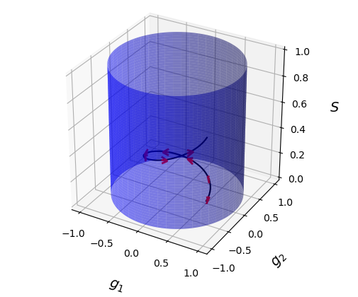
The matrix $G$ in Equation 11 is known to be positive definite, and $s$ is strictly positive. Therefore, our parameters are constrained to $\mathbb{R}_{+}\times B_{2}(r)$. The parameter space can be visualized as a solid cylinder extending infinitely far from the origin in one direction, as seen in Figure 1.

Figure 1: Parameter space for fitting an analytic profile, with sample iterations of the algorithm converging toward a learned $\left[s,g_{1},g_{2}\right]$. Note that the cylinder extends upwards toward infinity but is bounded from below by $0$.

We choose the following definition for ellipticity:

$$e_{i}=\frac{g_{i}}{1-||g||^{2}}.$$ (13)

This is a map from $B_{2}(r)\to\mathbb{R}^{2}$. We can construct an inverse map via

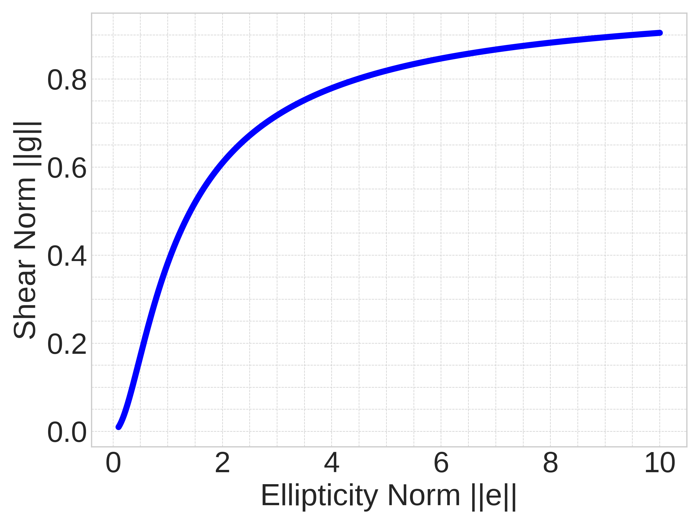
$$||g||=1+\frac{1}{2}\left(\frac{1}{||e||^{2}}-\sqrt{\frac{4}{||e||^{2}}+\frac{1}{||e||^{4}}}\right).$$ (14)

This inverse map allows us to constrain our update steps inside of our parameter space which leads to quicker convergence and the ability to handle noisier data more effectively. Equation 14 also keeps the nice properties of smoothness and monotonicity desirable for activation functions, see Figure 2. Equation 14 is not the canonical map from $\mathbb{R}^{2}$ to $B_{2}(r)$; two sigmoid functions could also have been used. We chose this particular function because it has the proprieties we want while retaining a geometric interpretation.

Note that this inverse only specifies what the new norm should be; the components still need to be adjusted accordingly. We reparameterize as follows:

$$s\equiv\sigma^{2}$$ (15)

$$g_{i}\equiv e_{i}\frac{||g||}{||e||}$$ (16)

The values of $\sigma,e_{1},e_{2}$ are obtained from each update step and $\lVert e\rVert$ is then determined from the usual $L_{2}$ norm. The parameter $s$ is obtained from Equation 15 and $\lVert g\rVert$ from Equation 14. Finally, $\lVert g\rVert$ is used with $\lVert e\rVert$ to calculate $g_{1}$ and $g_{2}$.

Figure 2: Reparameterization function. For any ellipticity vector $\left[e_{1},e_{2}\right]$ the associated shear vector $\left[g_{1},g_{2}\right]$ has a norm in $[0,1)$.

We have that $r$ is a function of $\left[u,v,s,g_{1},g_{2}\right]$ and $f$ is a function of $r$ such that

$$f(r)\equiv I_{p}(u,v,s,g_{1},g_{2}).$$ (17)

Even though we solve for parameters $\left[\sigma,e_{1},e_{2}\right]$, the loss is still dictated by $\left[s,g_{1},g_{2}\right]$.

$$\text{cost}(s_{t},g_{1_{t}},g_{2_{t}})=\frac{1}{2}\sum_{u_{pix}}\sum_{v_{pix}}(I_{p}(u,v)^{*}-I_{p}(u,v,s_{t},g_{1_{t}},g_{2_{t}}))^{2}$$ (18)

Here $*$ denotes the ground truth (i.e. star) in the star vignette and the subscript $t$ denotes iteration $t$ in an LBFGS run. Parameters are found using Julia’s Optim.jl library (Mogensen & Riseth, 2018) and the gradient is computed using Julia’s ForwardDiff.jl library (Revels et al., 2016).

3.2 Pixel Grid Fits

Both PCA mode and autoencoder mode provide “pixel-grid” mechanisms for reconstructing the PSF in the image pixel basis. We outline each of these modes below.

3.2.1 PCA Mode

PCA mode approximates a star image with a rank-$n$ approximation of the original image using principal component analysis, where $n$ is supplied by the user. Modeling the vignette in this way gives the user a method of determining how much they want their pixel grid model to represent the original star vignette. Choosing a lower rank approximation will yield less detail on the shape of the PSF, but will do so quickly and without much noise contamination. On the other hand, a higher rank approximation will capture more of the fine details, but at the risk of capturing some of the noise. It should be noted that the choice of $n$ has little overhead cost on the ShOpt computation time.

To minimize aliasing effects that might appear in low-rank approximations, the output image is convolved with a smoothing kernel $\mathcal{L}$:

$$\mathcal{L}(x,a)=\begin{cases}0&\text{if }|x|\geq a\\ 1&\text{if }x=0\\ a\text{sinc}(\pi x)\text{sinc}\left(\frac{\pi x}{a}\right)&\text{otherwise}\end{cases},$$ (19)

where $a$ is a tunable parameter for the size of the kernel and $x$ is the distance from the center of the kernel.

3.2.2 Autoencoder Mode

Autoencoder mode uses deep learning to reconstruct PSF vignettes pixel by pixel. We adopt an autoencoder architecture because the projection into a latent space forces the machine learning algorithm to learn the key features of the image regardless of the noise present. The operations are carried out by Julia’s Flux.jl machine learning library (Innes, 2018).

In our specific architecture, the input star vignette is first flattened and then passed through the network, which has an encoder with one layer containing $128$ nodes and a second layer containing $64$ nodes. The encoder feeds into a latent space with $32$ nodes, which is then decoded back into a layer of $64$ nodes, $128$ nodes, and finally back into an image (vignette) of the same dimension as the input vignette. We enforce both the input and output vignettes to sum to unity so that the relative distributions of intensities can be compared. The loss function is a mean squared error:

$$\text{cost}(x)=\frac{1}{N_{\mathrm{pix}}}\sum_{N_{\mathrm{pix}}}x_{p}-\hat{x}_{p},$$ (20)

where $\hat{x}$ denotes the image after it has been put through the autoencoder.

The network consists of two activation functions. A leakyrelu (Maas, 2013) function is used for all layers except for the last one. This choice reflects that most of the vignette pixel values are positive, and the ones that are not are usually close to zero or eliminated in data pre-processing. The final layer uses a tanh activation function to ensure that output values stay bounded between $(-1,1)$. The network trains until it either hits a specified number of epochs or until it hits a stopping gradient. We encourage exploration of the number of epochs and the minimum stopping gradient to find an appropriate middle ground between accuracy and time of completion. Stopping gradients between $10^{-5}$ and $10^{-6}$ are usually sufficient to get a good approximation in reasonable time and in $100$ epochs or less. This was revealed through the use of diagnostic plots that are introduced in 8. The activation functions and number of nodes are not tunable by default; changing those is not recommended.

4 Interpolation Across the Full Field of View

To fit for the spatial variation of the size and shape of the PSF, ShOpt first produces a rough estimate by interpolating the analytic fit parameters $\left[s,g_{1},g_{2}\right]$ across the field of view using a polynomial of order $n$, where $n$ is supplied by the user. For an order-$n$ polynomial $p(u,v))$, the cost function takes the form

$$\mathrm{cost}_{p}(\left[a_{0},\ldots,a_{(n+1)(n+2)//2}\right])=\left(\left[\sum_{(i,j),i+j\leq n}a_{ij}u^{i}v^{j}\right]-p(u,v)^{*}\right)^{2}$$ (21)

where $*$ denotes the ground truth obtained by pixel basis fits. This gives us different polynomials in $u$ and $v$ for $\left[s,g_{1},g_{2}\right]$. As elsewhere, the minimum of the cost function is found with LBFGS and the Optim.jl library.

Subsequently, the pixel-grid model is interpolated across the field of view. By definition, each pixel in pixel-grid models is a basis element, so the natural extension of Equation 21 is to give each pixel in an $n\times n$ vignette its own polynomial. There is a tunable parameter for the stopping gradient that leaves the tradeoff between speed and accuracy of the polynomial interpolation to the end user.

Not all stars are good exemplars of the PSF due to things like saturation, color effects, and noise. To combat this, ShOpt does its polynomial interpolation over several iterations according to Algorithm 2.

Algorithm 2 Iterative Polynomial Interpolation and Star Filtering Process

NumIterations $\leftarrow$ [define number of iterations]

2:for $i\leftarrow 1$ to NumIterations do

     PSFModel $\leftarrow$ PolynomialInterpolate(TrainingStars)

4:     RenderedStars $\leftarrow$ RenderPSF(PSFModel)

     MSE $\leftarrow$ ComputeMSE(TrainingStars, RenderedStars) $\triangleright$ MSE: Mean Squared Error

6:     WorstStars $\leftarrow$ GetWorstPerformingStars(MSE, 10%)

     TrainingStars $\leftarrow$ TrainingStars - WorstStars

8:end for

FinalPSFModel $\leftarrow$ PolynomialInterpolate(TrainingStars)

10:return TrainingStars, FinalPSFModel

The number of iterations to refine the polynomial interpolation is specified by the user. After each iteration, the predicted PSF is rendered at each star location and the mean squared error (Equation 22) is computed using the training stars. The worst $10\%$ of training stars are filtered out.

$$\text{Mean Squared Error}=\frac{1}{N_{\mathrm{pix}}}\sum_{(i,j)}^{N_{\mathrm{pix}}}(v_{i,j}-p_{i,j})^{2}$$ (22)

Polynomial interpolation for high-degree polynomials can be the most expensive part of the whole PSF fitting procedure. For this reason, ShOpt is strict about filtering outliers in polynomial interpretation. Training stars are excluded based on the value of $s$ that was found during the analytic-profile interpolation step, which eliminates the need for additional iterations to clean the training data. Additionally, we make the conscious decision not to continue filtering our training stars until we reach a given $n\sigma$ confidence. The JWST PSFs contain lots of background noise between the “wings” of the stars we are trying to model. Consequently, an excessive number of iterations may be required to reach the desired level of confidence.

5 Data pre-processing and outlier rejection

In ShOpt’s outlier rejection process, three distinct phases are employed: (1) SNR-based filtering on input stars; (2) a Gaussian fit size filter on the input stars; and (3) a separate Gaussian fit size filter on pixel grid models. Following these phases, the process advances to the iterative refinement for polynomial fitting, as detailed in Section 4.

Before doing anything else, ShOpt filters out bad stars on the basis of SNR; the default SNR metric is the SExtractor SNR_WIN parameter. By default, ShOpt filters out the noisiest 33% of entries, a percentage determined through experimentation. Users can adjust this threshold to fit their specific data sets. ShOpt also has an alternative calculation for SNR,

$$SNR=\log_{10}\frac{\sum^{N_{\mathrm{pix}}}\left(I_{\mathrm{pix}}\right)^{2}}{\sum^{N_{\mathrm{pix}}}\left(\sigma_{\mathrm{pix}}\right)^{2}}$$ (23)

where $\sigma_{\mathrm{pix}}$ comes from the error extension of NIRCam image files. This ERR extension comes from the combined VAR_POISSON and VAR_RNOISE data and is expressed as a standard deviation. While this formulation yields a more interpretable SNR distribution, it relies upon a specific (NIRcam) image file format, and so is not presently implemented.

The remaining vignettes are then fit with a multivariate Gaussian, as described in Section 3. We filter again based on the object size $s$. A very small or very large $s$ probably corresponds to objects that are not point sources. By default, vignettes with $s<0.075$ or $s>1$ are filtered out. This ensures further computation time is not wasted on bad data. We apply the same size filtering after fitting Gaussians to the pixel grid models. This prevents poor pixel grid models from being used in our polynomial interpolation, as mentioned in Section 4.

ShOpt also offers several methods for efficiently cleaning useful data without discarding it. Given that SExtractor sets the flux of interloping sources to a sentinel value of $-10^{-32}$, ShOpt sets pixels less than $-1000$ to NaN. Before doing any analytic or pixel grid fits, we also smooth the image according to the kernel introduced in Equation 19 to avoid any hot pixels in the vignettes. Finally, we recommend that users select true in the yaml configuration for the setting sum_pixel_grid_and_inputs_to_unity. This enforces intensity to sum to unity in each of our model vignettes and their pixel grid fits.

6 Runtime Analysis

In this section, we compare the $\mathcal{O}(n)$ algorithmic complexity and convergence properties of ShOpt, PIFF and PSFEx, examining the analytic profile fits, pixel grid fits, and polynomial interpolation steps separately. Runtime analysis of the three PSF fitters allow us to argue for the algorithmic choices implemented in ShOpt without needing to factor in programming language or computing power. The results will serve as predictions for the speed tests of Section 8.2.

6.1 Analytic Profile Fit Runtime

Let $n$ denote the number of pixels on one side of a square vignette, so that there are $n^{2}$ total pixels. In our optimization scheme, we compute the loss between every pixel in the vignette and the analytic profile prediction an average of $I$ times. Our nominal runtime is thus $\mathcal{O}(n^{2}\times I)$. We may safely assume for large $n$ that $n^{2}\gg I$, leaving us with $\mathcal{O}(n^{2})$. So, in the case of large $n$, all PSF fitters should be comparable regardless of their method for finding $\left[s,g_{1},g_{2}\right]$ because the run time is mostly determined by the size of the vignettes.

Different considerations apply when $n$ is not large. PIFF solves for $\left[s,g_{1},g_{2}\right]$ using conjugate gradient descent, a technique that relies on linear approximations to find the optimal direction of improvement (Jarvis et al., 2020). On the other hand, ShOpt uses LBFGS, which uses super-linear approximations to calculate the direction of improvement. Since each iteration of LBFGS should take us closer to the solution than conjugate gradient descent, we should expect LBFGS to take fewer steps on average to compute. The LBFGS algorithm and the reparameterization step introduced in Section 3.1 allows us to argue that $I_{ShOpt}<I_{PIFF}$. That is to say, in the case where $n$ is small enough, ShOpt will on average converge to the correct $\left[s,g_{1},g_{2}\right]$ faster than PIFF because ShOpt uses a more memory expensive technique to compute its update steps and does it in such a way that keeps the solution within a constraint.

6.2 Pixel Grid Fit Runtime

6.2.1 PCA Mode

Principal component analysis relies on computing the singular value decomposition of the covariance matrix of a given data set. Singular value decomposition is typically $\mathcal{O}(n^{3})$ for an $n\times n$ matrix, but for an approximation using the first $k$ principal components, the fit is typically much cheaper to compute; this brings the calculation closer in complexity to the $\chi^{2}$ minimization pixel-grid fitting implemented in PIFF and PSFEx (Bertin, 2011; Jarvis et al., 2020).

6.2.2 Autoencoder Runtime

As in 6.1, we may observe that the complexity is $\mathcal{O}(n^{2}\times I)$ because the loss is computed an average of $I$ times over $n^{2}$ pixels. The number of parameters between layers as a function of neurons $m$ in layer $i$ in our network is given by

$$N_{params}=\left(m_{i-1}\times m_{i}\right)+m_{i}$$ (24)

where the first term corresponds to the number of weights and the second term corresponds to the biases. In our network the number of nodes for the input and output is set by a flattened version of the input image. Therefore, the number of parameters to learn grows as $\left[\left(n^{2}\times 128\right)+128\right]+\left[\left(128\times n^{2}\right)+n^{2}\right]$. On the other hand, PIFF and PSFEx employ a form of $\chi^{2}$ minimization, wherein each pixel in the image is a learnable parameter; for an $(n,n)$ image there are only $n^{2}$ learnable parameters and $n^{2}$ pixels computed in the loss function. Even though the loss function in ShOpt is also computed over $n^{2}$ pixels, there are much more than $n^{2}$ learnable parameters, so we expect the autoencoder to take more iterations to converge on average than PIFF and PSFEx. For this reason, autoencoder is not the default mode for pixel grid fits in shopt. It should be reserved for cases that demand precision and where the images are small enough to be learned efficiently so the transfer learning effect is more pronounced.

6.3 Polynomial Interpolation Runtime

Almost all PSF fitting software makes use of polynomial interpolation to model the variation of the PSF across the camera’s field of view. Any performance gains in this area are primarily derived from the efficiency of the polynomial fitting process to the data. In PSFEx, these fits are implemented using PCA, which Bertin (2011) argues requires the lowest number of basis vectors to approximate an image if the data is sufficiently well-behaved.

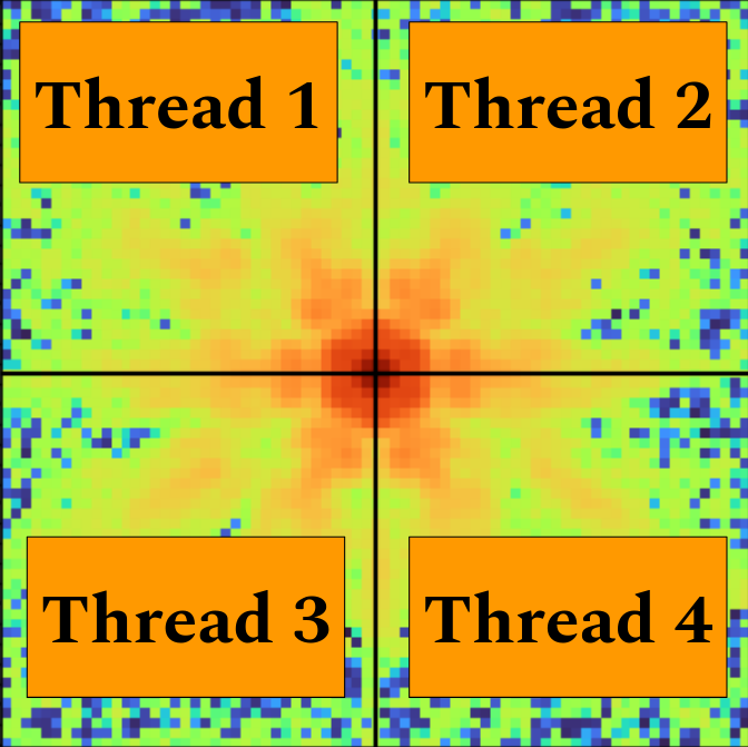
In ShOpt, we opt for a nonlinear approach, using LBFGS to fit each pixel with an independent polynomial. This process is inherently parallelizable because the polynomial found for one pixel is independent of the polynomial found for any other pixel. ShOpt will automatically use as many threads are made available to it. The idea to break these operations into computation blocks is inspired by Tiny Machine Learning problems described in Sabot et al. (2023) and the CAKE algorithm outlined in Kung et al. (2021). Currently, the number of threads is not configurable because it has to be specified before the program is run. On UNIX, we ran export JULIA_NUM_THREADS=4 before running the program, on Windows you can similarly run set JULIA_NUM_THREADS=4.

Figure 3: Pictoral representation of multi-threading in ShOpt. In this example, all of the pixels in the upper left of the pixel grid renderings are interpolated across the field of view in thread $1$, all of the pixels in the upper right of the pixel grid renderings are interpolated across the field of view in thread $2$, and so on.

6.4 Order of Operations

We are also deliberate about the order of operations in ShOpt. The initial analytic profile fitting serves as a data cleaning method, which allows us to not waste compute time fitting pixel-grid models to outlier stars. A second round of analytic profile fits to the resulting PSF models further refines the data set, ensuring that the (computationally expensive) polynomial interpolation is applied only to the highest quality PSF models. By contrast, PIFF adopts an integrated approach where analytic and pixel grid fits are interwoven with iterations of polynomial interpolation. While this method is thorough, our approach is designed to prioritize computational expediency.

7 Benchmarking, Data, and Analysis

Our PSF analysis utilizes NIRCam imaging from the COSMOS-Web survey (Casey et al., 2023), which we have chosen for its expansive coverage (more than three times the area of all other JWST surveys combined) in four bandpasses as well as the fact that many of its science cases require careful PSF characterization. This section presents an overview of the three COSMOS-Web data sets employed in our PSF benchmarking analysis—simulated single exposures, simulated observation mosaics, and real observation mosaics—followed by a description of the benchmarking methods we apply to each.

We employ simulated observations for PSF code unit testing because they provide a controlled environment with fully known input parameters. Unlike real observations, simulations allow for us to control for observational imperfections such as saturation, noise, or defective pixels; this allows for the establishment of a ground truth against which the accuracy of PSF model fits can be measured directly. Although real observations feature the true PSF and are integral to our study, their inherent uncertainties and the absence of a definitive PSF ground truth make them less suitable for initial code validation. Instead, the real data serves as a stress-test for the PSF fitting codes, ensuring they remain effective when confronted with the vagaries of real observations.

1. Simulated Data: These simulations are based on the COSMOS 2020 data (Weaver et al., 2022), and contain all the known galaxies and stars in this field. Galaxy fluxes in JWST filters were calculated from Stardust SEDs if they existed (Kokorev et al., 2021); otherwise, fluxes were found by interpolating across existing photometry in other filters. Star fluxes were similarly modeled by interpolating available photometry. Galaxies with counterparts in the Zurich Structure & Morphology catalog (Scarlata et al., 2007; Sargent et al., 2007) were assigned the according morphological parameters (Sérsic indices, ellipticity, position angle, size), or from observed distributions if they did not.

   COSMOS-Web-like NIRCam images were generated using the Multi-Instrument Ramp Generator (MIRAGE; Hilbert et al., 2019), which includes PSF modeling with WebbPSF (Perrin et al., 2014), sky background, detector noise, dark current, and Poisson noise. After the images were generated, the JWST calibration pipeline (Bushouse et al., 2023) was used to reduce the raw NIRCam data and create mosaics, with some modifications, like 1/f noise and subtraction of low-level background (e.g., Finkelstein et al., 2022; Bagley et al., 2022). We employ two sets of simulated images:

   1. Simulated Single Exposures: Stars are generated by convolving a MIRAGE WebbPSF model with an idealized point sources, so these images allow us to measure success directly by comparing the learned PSF to the input PSF. We employ images from stage 2 of the JWST calibration pipeline, so there are no effects from dithering or distortion (i.e., tweakreg). The main challenge in using this data is low star density, particularly for the short wavelength channel. With a training/validation split of $90\%$, this led to an average of $1$ validation star for each subarray in the F115W filter, $1$ validation star for the F150W filter, $2.2$ stars for the F277W filter, and $2.3$ stars for the F444W filter. To gather enough data for meaningful summary statistics, we combine exposures from visits $\{43,44,45,46,47,48\}$.

   2. Simulated Mosaics: Image mosaics are i2d-format data cubes built from single exposures that have passed through stage 3 of the JWST science calibration pipeline.

      As such, the mosaics do reflect normal dithering and distortion effects. The simulated mosaics used in our study cover a contiguous area of 76 arcmin² at the full COSMOS-Web depth ($\sim 27th$ magnitude) and provide a reasonable 0.5 star per square arcminute.

   For an in-depth discussion of the simulation process, refer to Drakos et al. (in prep).

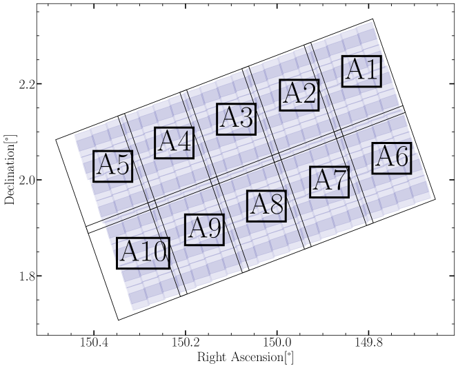
2. Real Mosaics: The real data used in our analysis was taken in April 2023 and includes visits $77-152$, covering $0.28$ deg² in the bottom right of our allocated area of the COSMOS field (Casey et al., 2023) program ID 1727. Three of the planned visits were skipped, so the data includes a total of $72$ visits. As with the simulated mosaics, we use the i2d-format data cubes produced by stage 3 of the JWST science calibration pipeline. We restrict ourselves to an approximately $0.11$ deg² area of the full field of view, corresponding to tiles $\{A1,A5,A6,A10\}$ in Figure 4; we chose these particular tiles to test the relative performance of the PSF fitters where we expect astrometric distortions to be the most severe.

Figure 4: April data tiling scheme.

Our benchmarking procedure has four steps:

1. Run Source Extractor (SExtractor) on our images to generate star catalogs (Bertin & Arnouts, 1996). For the simulated data, stars are identified by matching the SExtractor catalogs the input point source catalogs. For real data, star catalogs are created using cuts on the stellar locus, an example of which is shown in Figure 5. The config file for SExtractor is given in the Appendix. Note that we run source extractor on the individual tiles and aggregate our results over all of them.

   

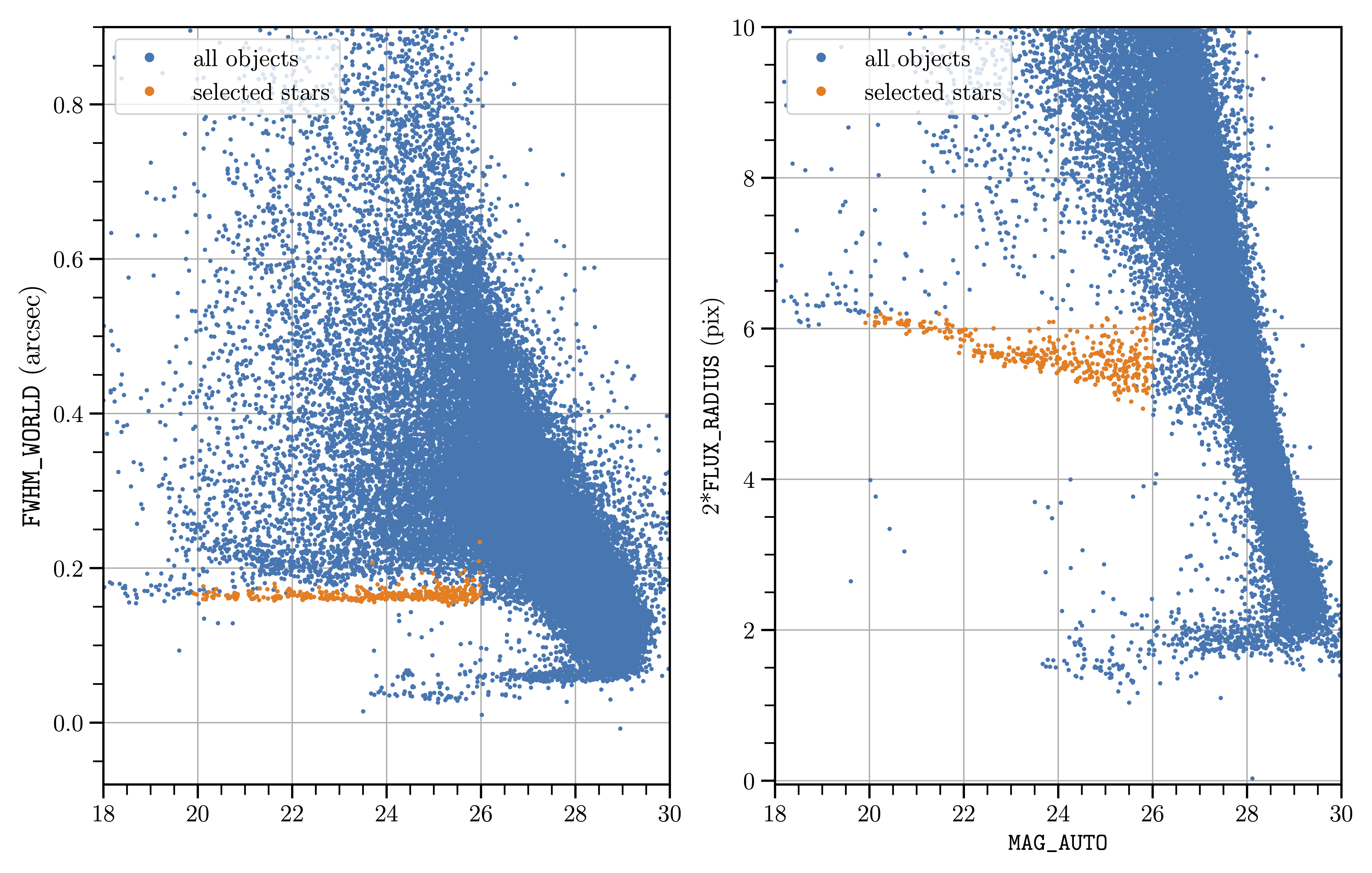
   Figure 5: Size-magnitude diagram for objects detected in the A6 mosaic in F444W A6. Blue points represent all sources; orange points show stars selected by stellar locus parameter cuts.

2. The resulting star catalogs are segregated into training (90%) and validation (10%) catalogs. We are careful to filter out saturated stars in our catalogs by searching for sentinel values of $0$ in the ERR extension (for i2d-format mosaics) or ${1,2}$ in the DQ extension (for single exposures). Vignettes that contain any pixels set to a sentinel value are removed from the catalogs.

3. We use the training catalogs to get empirical PSF models for each fitter. We run ShOpt (Berman & McCleary, 2023), PIFF (Jarvis et al., 2020), and PSFEx (Bertin, 2011).

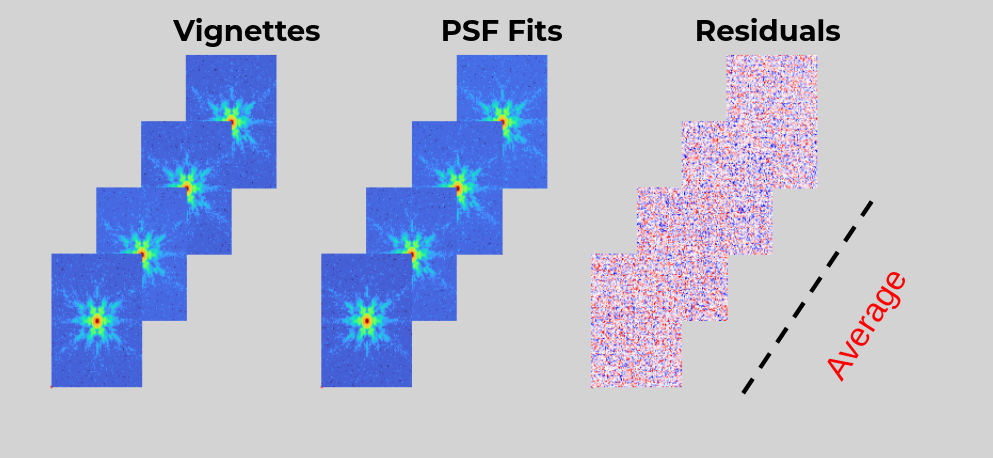
4. We then use the reserved validation star catalogs to calculate the summary statistics of Equations 5–8. Figure 6 illustrates this process: we calculate the residuals between the star vignettes (or MIRAGE cutouts for simulations) and renderings of the PSF models, then take the mean. To obtain single residual scores, we compute the mean and standard error of all pixels in residual images.

Figure 6: Schema illustrating the computation of summary statistics for PSF model assessment. Individual star-PSF model pairs are compared to produce residual images, which are then averaged into a mean residual image for the ensemble.

The code for creating star catalogs, calculating statistics, and creating the associated PSF diagnostic figures can be found on GitHub.

8 Results

In this section, we report the outcomes of the PSF benchmarking analysis detailed in Section 7. The comprehensive PSF model fidelity analysis is presented in Section 8.1, and the assessment of the computational efficiency of the different PSF fitters is presented in Section 8.2.

We note that ShOpt was run in PCA mode throughout, with an optimal number of PCA terms established through direct experimentation. We found that the alternative, Autoencoder mode, took longer to run without enhancing the PSF model quality. Appendix C contains representative configuration files supplied to each PSF fitter.

8.1 Model Fidelity

As described above, we evaluate the relative performance of PSF models produced by PIFF, PSFEx, and ShOpt using mean and median reduced $\chi^{2}$ residuals, the MRE, and the MAE (cf. Equations 5–8). These statistics are computed using the reserved validation stars, which number from 35 for the simulated F277W and mosaics to 156 for the F150W real mosaics (Table 1). Statistics and diagnostic plots are based on PSF vignette sizes of $(75,75)$ pixels, which encloses the majority of the relevant star and PSF light profiles without including excessive sky background or a large number of interloping objects.

Data Type	Filter	Validation Stars
Simulated single exposures	F115W	83
	F150W	81
	F277W	107
	F444W	109
Simulated mosaics	F115W	37
	F150W	79
	F277W	35
	F444W	35
Real mosaics	F115W	155
	F150W	156
	F277W	148
	F444W	136

Table 1: Number of reserved validation stars for the three imaging data sets under consideration in each of the four COSMOS-Web NIRCam bandpasses.

8.1.1 Simulated single exposures

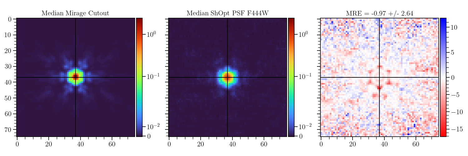
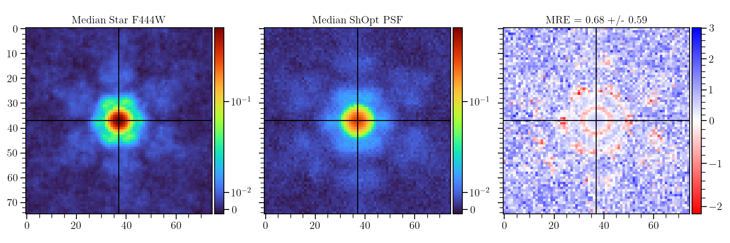
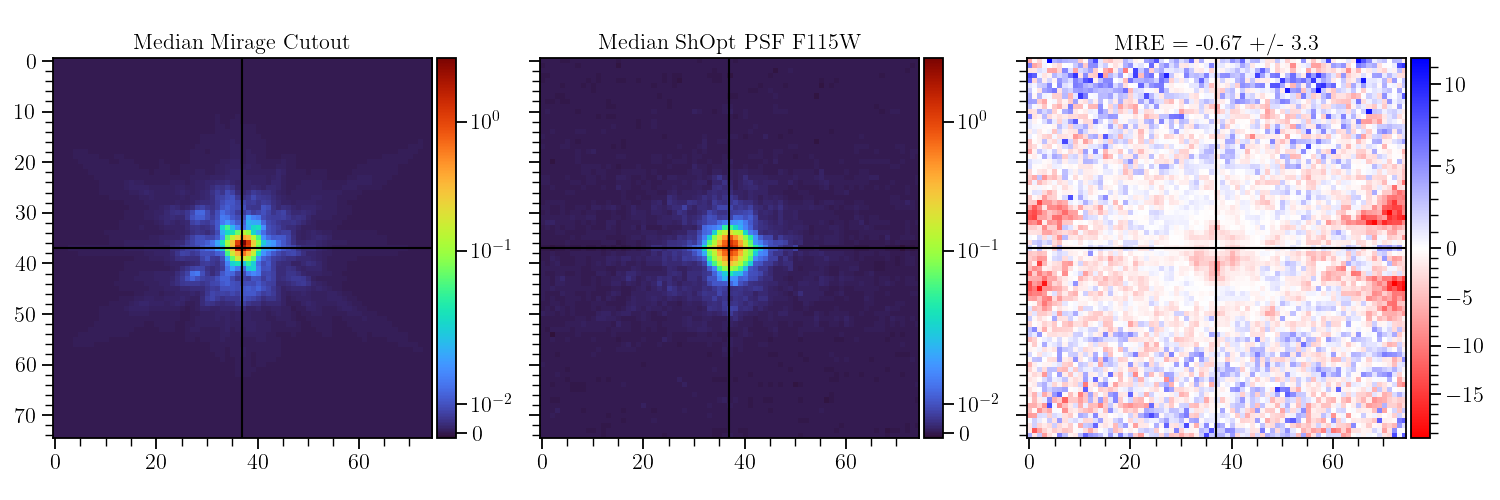
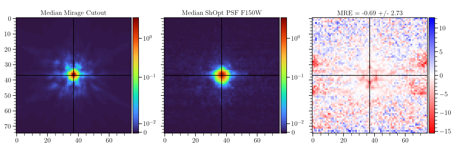
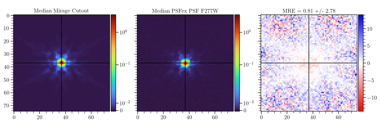
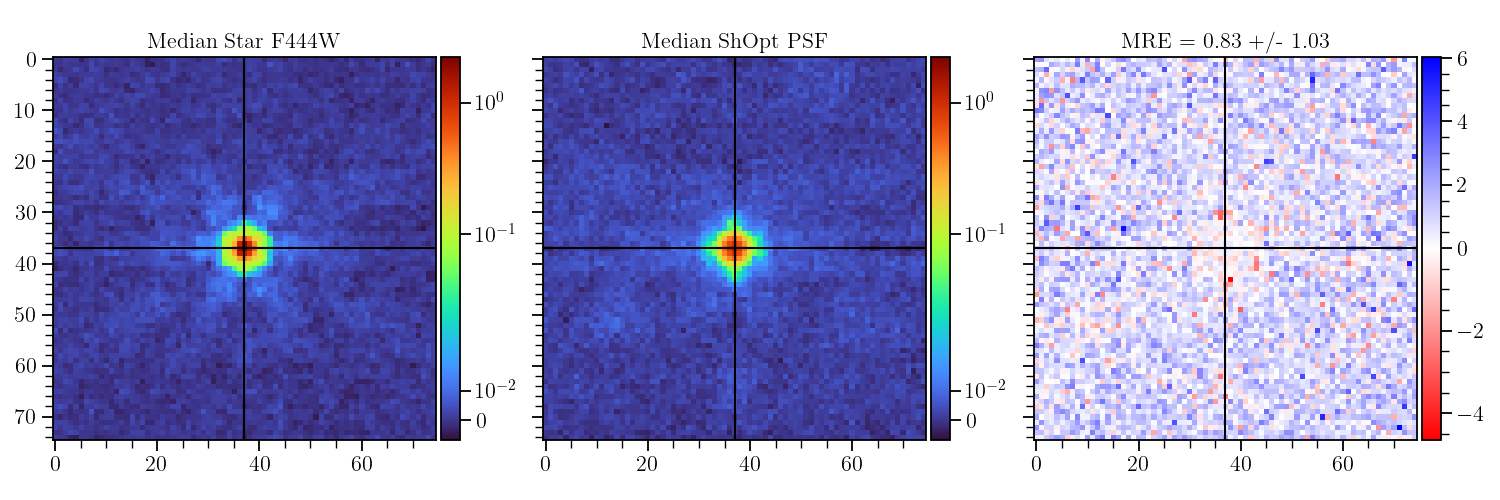
Despite the sparsity of training data for simulated single exposures, Figures 7, 19, and 20 show that both PSFEx and ShOpt can produce models of the central region of the PSF. The mean relative errors displayed in Figures 7, 19, and 20 are consistent with zero for both ShOpt and PSFEx, and the distributions of reduced $\chi^{2}$ shown in Figures 8 and 9 overlap in all four bandpasses. Ordinarily, these statistics would suggest that ShOpt and PSFEx perform equally well at fitting PSF models to single NIRCam exposures. However, the actual values of the statistics are high: the mean reduced $\chi^{2}$ ranges from 10 to 29—suggesting that the models fail to fully capture the underlying PSF—and the standard deviations of the MRE are also quite large. Figures 7, 19, and 20 show that both ShOpt and PSFEx models tend to be over-concentrated at the hexagonal perimeter of the core, which shows up as red (oversubtracted) regions in the right-hand panels of the figures. This tendency to excess concentration is more pronounced in the ShOpt models, particularly the F444W bandpass model shown in Figure 7. The background noise in ShOpt’s learned models tends to be high, which manifests as higher variance towards the edges of the image in the mean residual images. This variance is consistent across the FOV and suggests that the issue is with the low number of training PSFs and the modeling of each. The shorter-wavelength ShOpt models of Figure 19 shows an additional artifact: horizontal banding that does not exist in the input MIRAGE PSFs.

We do not test PIFF on the simulated single exposures, as the weight map format required by PIFF is not included in the default format of stage-2 calibrated (cal) NIRCam exposures.

Figure 7: Mean relative error between MIRAGE input point source images and PSF models for the F444W filter. Left panels show the median MIRAGE cutout; center panels show the median PSF cutout. Right panels show the average relative error between the MIRAGE and PSF cutouts. Top two rows are ShOpt, bottom two rows are PSFEx. Color bars for left and center panels show pixel intensity values in units of MJy/str. Color bars in the right panels show the (dimensionless) relative error. The MREs defined in Equation 7 are displayed in the titles of the mean residual images.

Figure 8: Confidence intervals of $\overline{\chi^{2}}$ for simulated single exposure data as a function of bandpass. PSFEx values are shown in red; ShOpt values are shown in green. Here and below, error bars show the standard deviation about the mean values.

Figure 9: Distribution of $\chi^{2}$ for simulated single exposure images. Not shown are two PSFex $\chi^{2}$ values greater than $100$ and three ShOpt $\chi^{2}$ value greater than $100$.

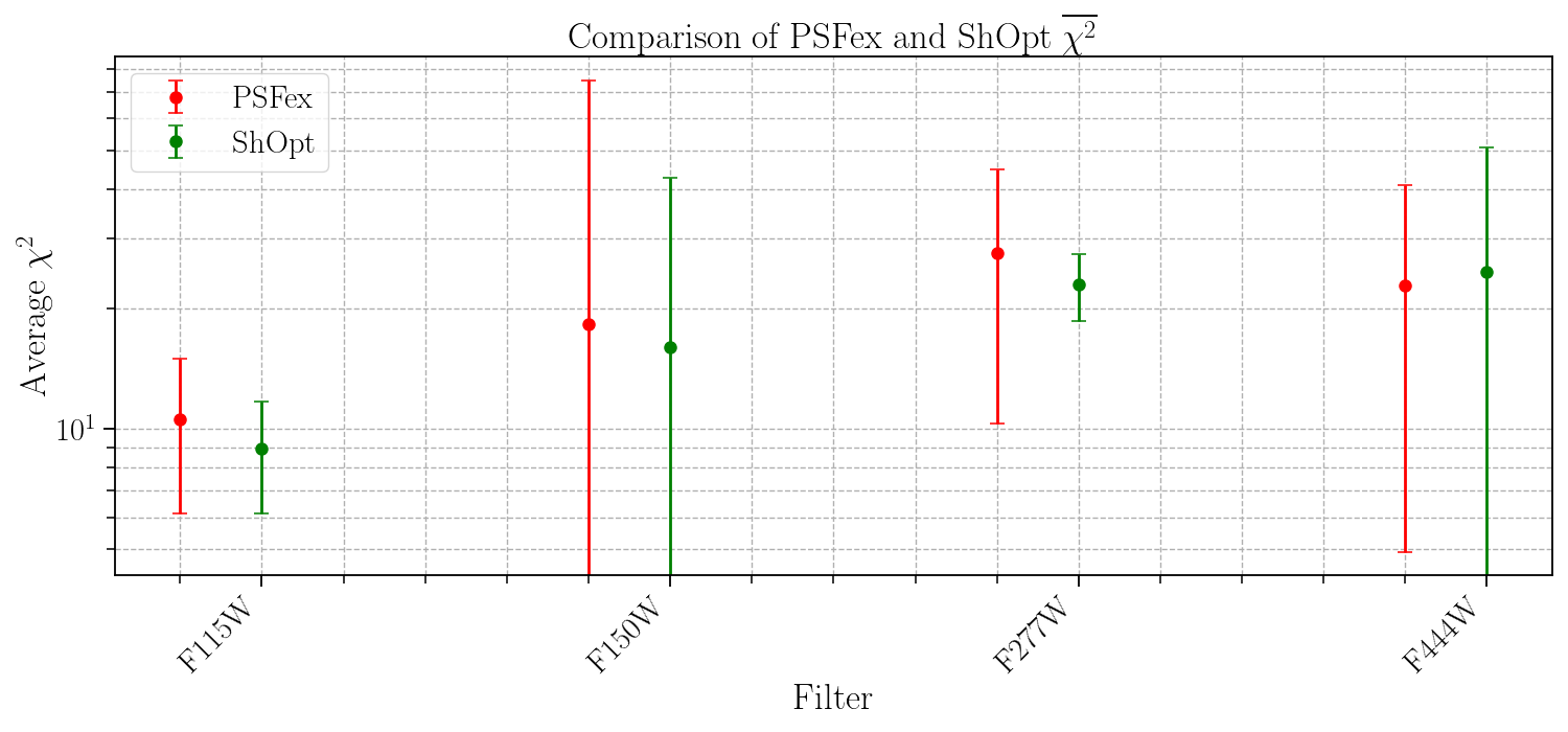
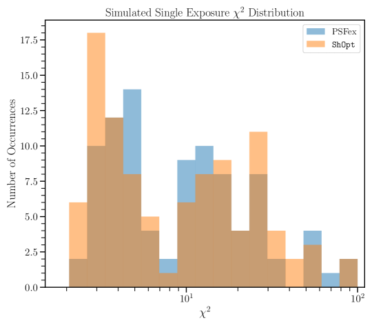
8.1.2 Simulated mosaics

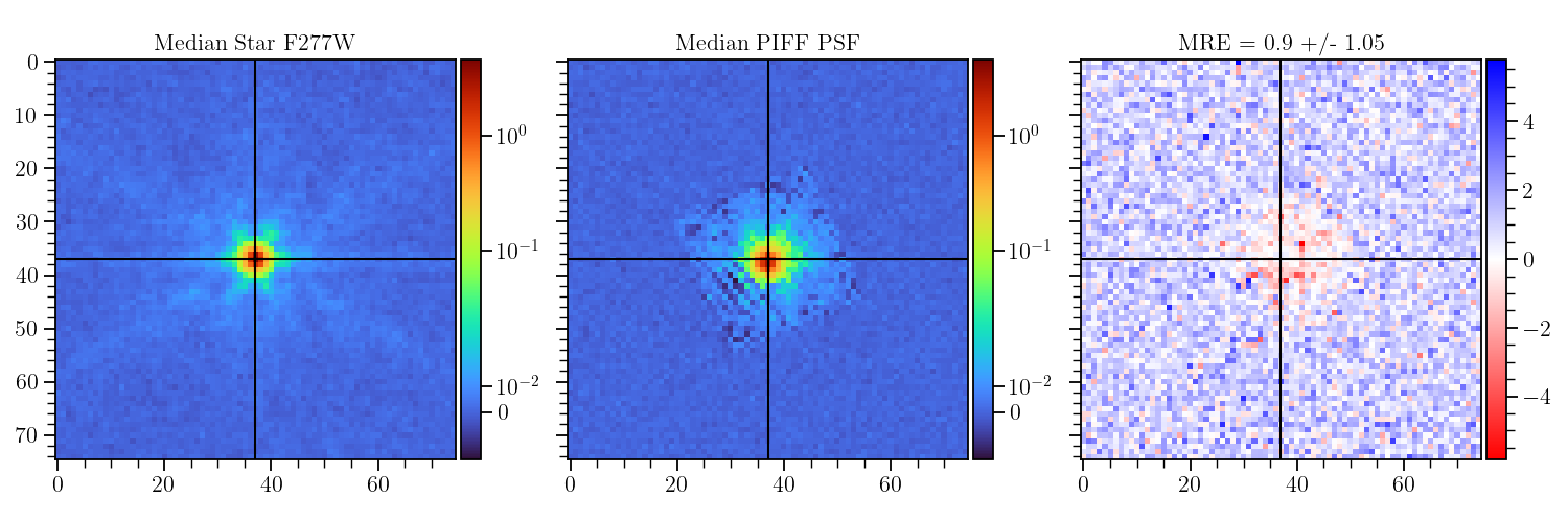
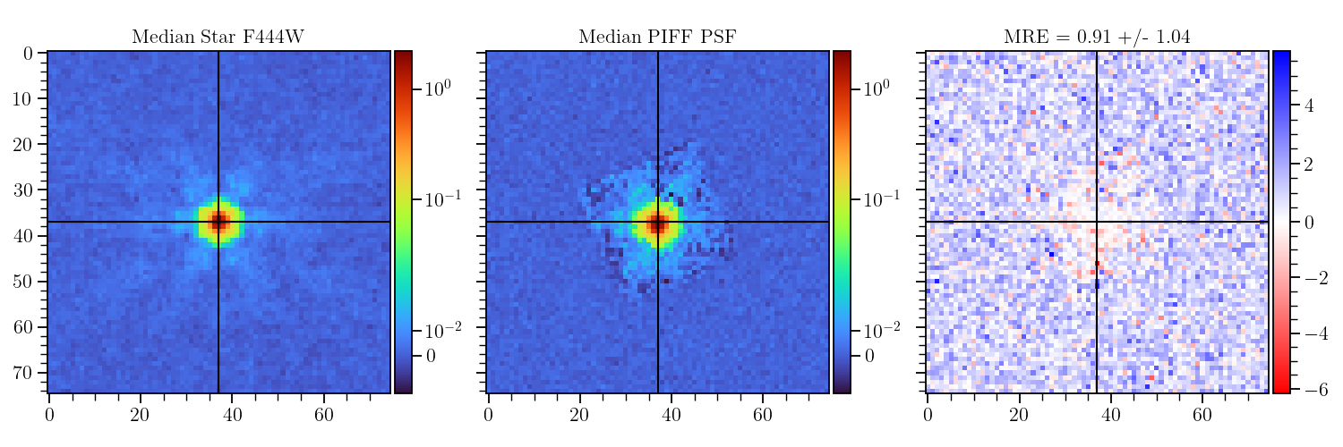
The simulated data mosaics have a higher density of training stars, as evinced by significantly better fits for PSFEx and ShOpt than the simulated single exposures. We also supply PIFF fits for these images, as the i2d-format mosaic data cubes include a weight map in the appropriate format for PIFF.

All PSF fitters yield models of better quality than were produced from the simulated single exposures. Figures 10 and 21–23 do not show the same central over-concentration visible in Figures 7, 19, and 20, and this set of ShOpt models is free from the horizontal banding artifacts that marred the single-exposure models.

Filter	PSF Fitter	MAE	MRE	$\overline{\chi^{2}}$	Median $\chi^{2}$
F115W	ShOpt	2.81$\pm$1.02	0.74$\pm$1.00	8.11$\pm$3.90	2.09
	PIFF	3.12$\pm$1.29	0.87$\pm$1.20	12.76$\pm$6.34	2.04
	PSFex	2.66$\pm$0.96	0.81$\pm$0.94	3.83$\pm$1.26	1.86
F150W	ShOpt	2.83$\pm$0.71	0.84$\pm$0.68	5.66$\pm$16.19	1.57
	PIFF	2.87$\pm$0.76	0.88$\pm$0.72	5.98$\pm$19.84	1.40
	PSFex	2.69$\pm$0.67	0.87$\pm$0.64	5.41$\pm$26.82	1.30
F277W	ShOpt	2.89$\pm$1.04	0.81$\pm$1.03	22.85$\pm$65.13	2.32
	PIFF	2.74$\pm$0.92	0.85$\pm$1.06	36.96$\pm$110.12	1.91
	PSFex	2.67$\pm$0.95	0.83$\pm$0.96	16.74$\pm$42.12	1.90
F444W	ShOpt	2.92$\pm$0.99	0.84$\pm$1.05	6.88$\pm$13.59	2.15
	PIFF	2.83$\pm$0.97	0.89$\pm$1.05	6.05$\pm$10.66	1.88
	PSFex	2.75$\pm$0.92	0.86$\pm$1.00	2.24$\pm$1.90	1.40

Table 2: Simulated mosaic summary statistics.

Figure 10: Evaluation of mean relative error between stars and PSF models for simulated mosaics in the F150W bandpass. Left panels show the median of the vignettes. Center panels show the median PSF cutout. Right panels show the average relative error between the vignette cutouts and the PSF cutouts. Top is PSFEx, middle is ShOpt, bottom is PIFF.

Figure 11: Confidence of $\overline{\chi^{2}}$ for simulated data mosaics. PSFEx values are shown in red, ShOpt values are shown in green, and PIFF values are shown in blue.

Figure 12: Distribution of $\chi^{2}$ for simulated data mosaics. PSFEx values are shown in blue, ShOpt values are shown in orange, and PIFF values are shown in green. For clarity, the plot excludes two PSFex $\chi^{2}$ values greater than $100$, one ShOpt $\chi^{2}$ value greater than $100$, and two PIFF $\chi^{2}$ values greater than $100$.

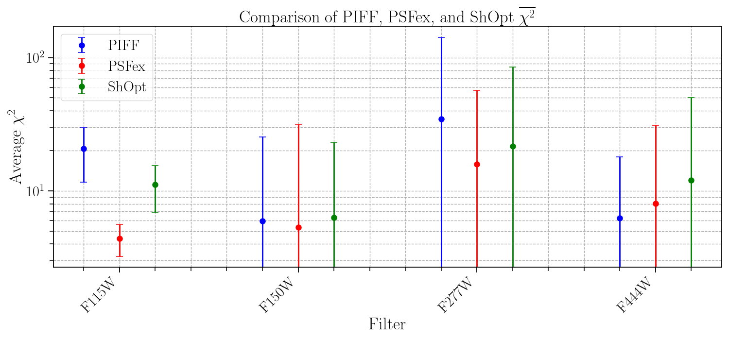
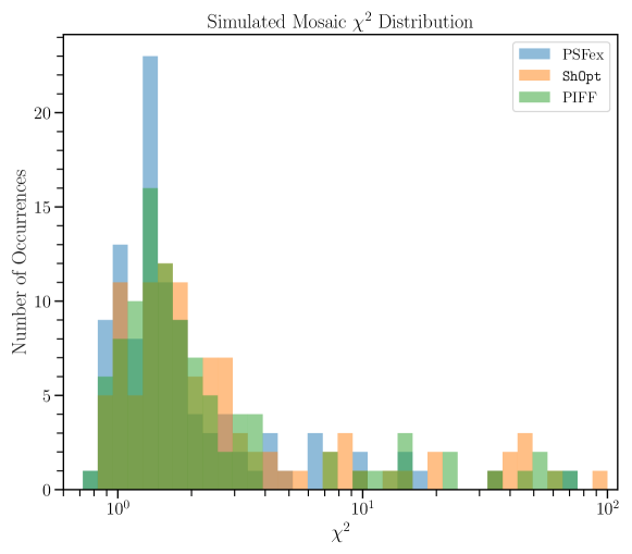
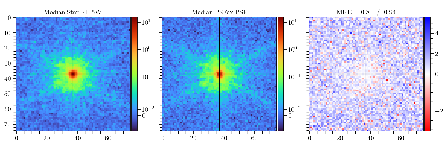
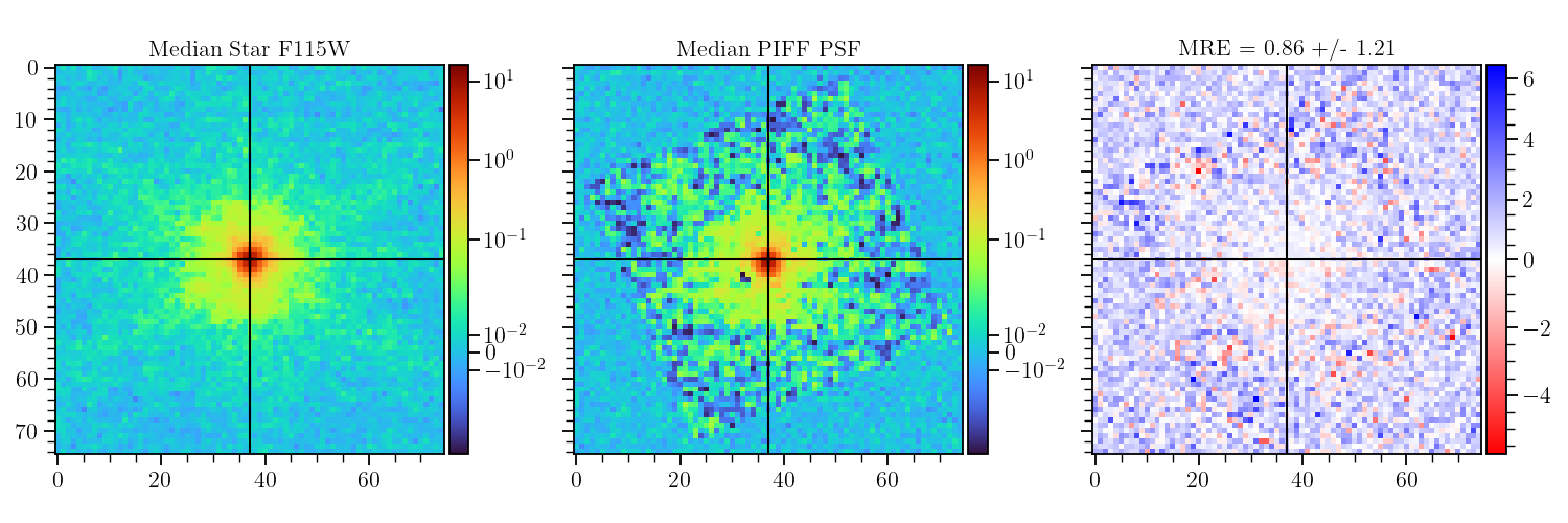
Figures 11 and 12 suggest minimal statistical difference in performance among the PSF fitters, with the notable exception of the F115W filter where PSFEx outperforms PIFF, as reflected by a lower $\overline{\chi^{2}}$.

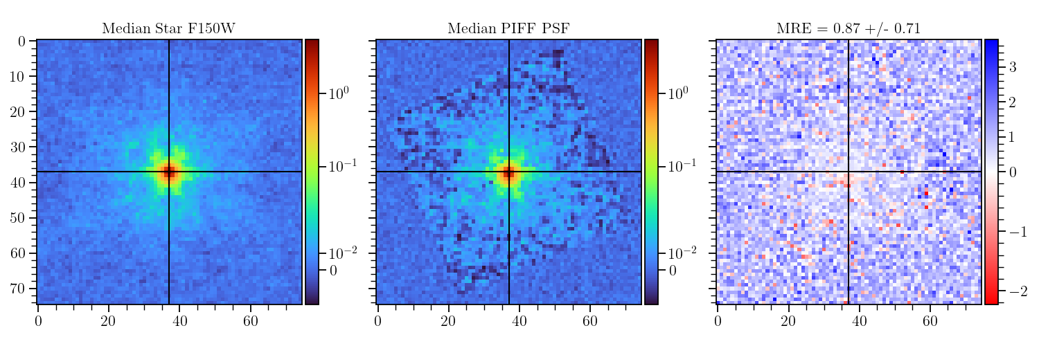
Table 2 shows MRE and MAE values are consistent with zero for all ShOpt and PSFEx models, suggesting minimal bias. While the PIFF model residuals are also consistent with zero, the large standard deviations indicate a high variability in the quality of PIFF PSF fits.

In general, the presence of outlier fits obscures a clear ranking based on MAE, MRE, and $\overline{\chi^{2}}$ alone. The median $\chi^{2}$ and its distribution, as shown in Figure 12 and Table 2, seem to be more indicative of performance, demonstrating no significant difference in the reliability of the PSF fitters for the simulated mosaics.

8.1.3 Real mosaics

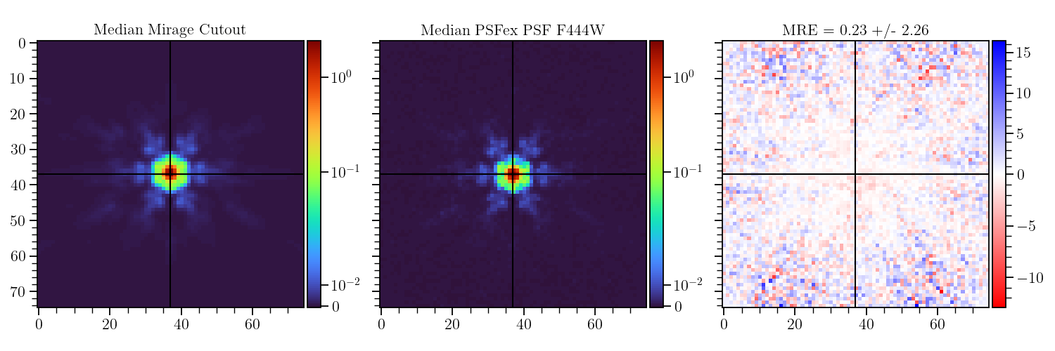
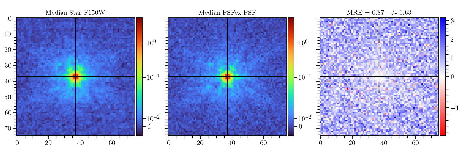
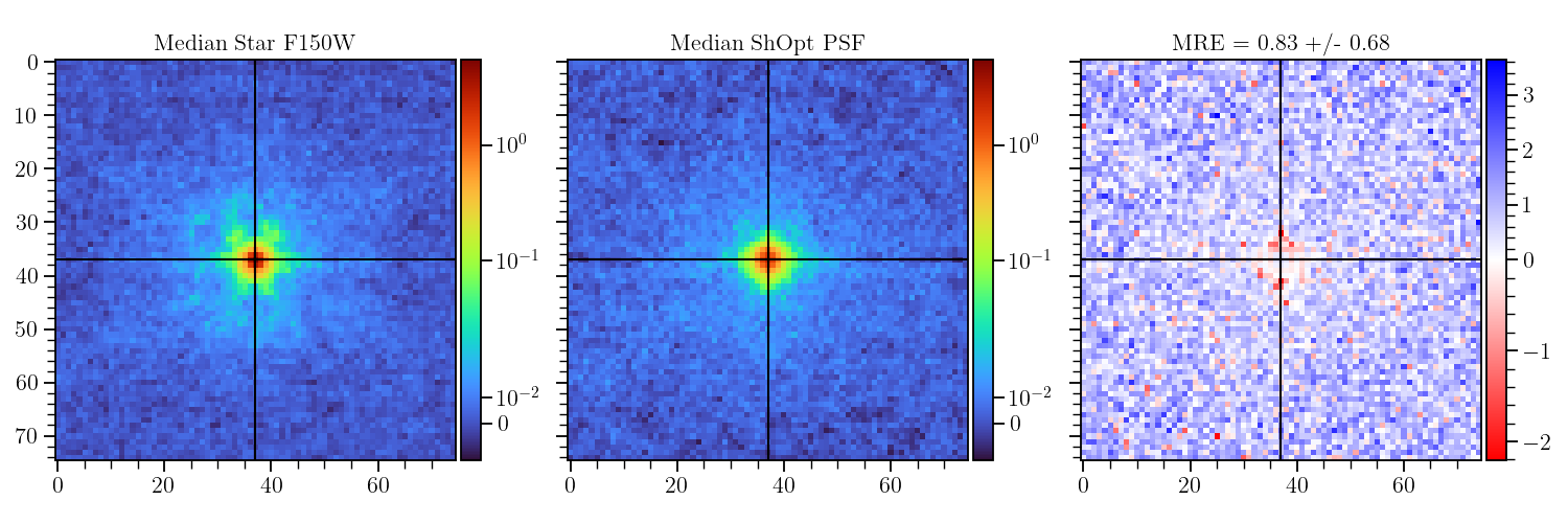
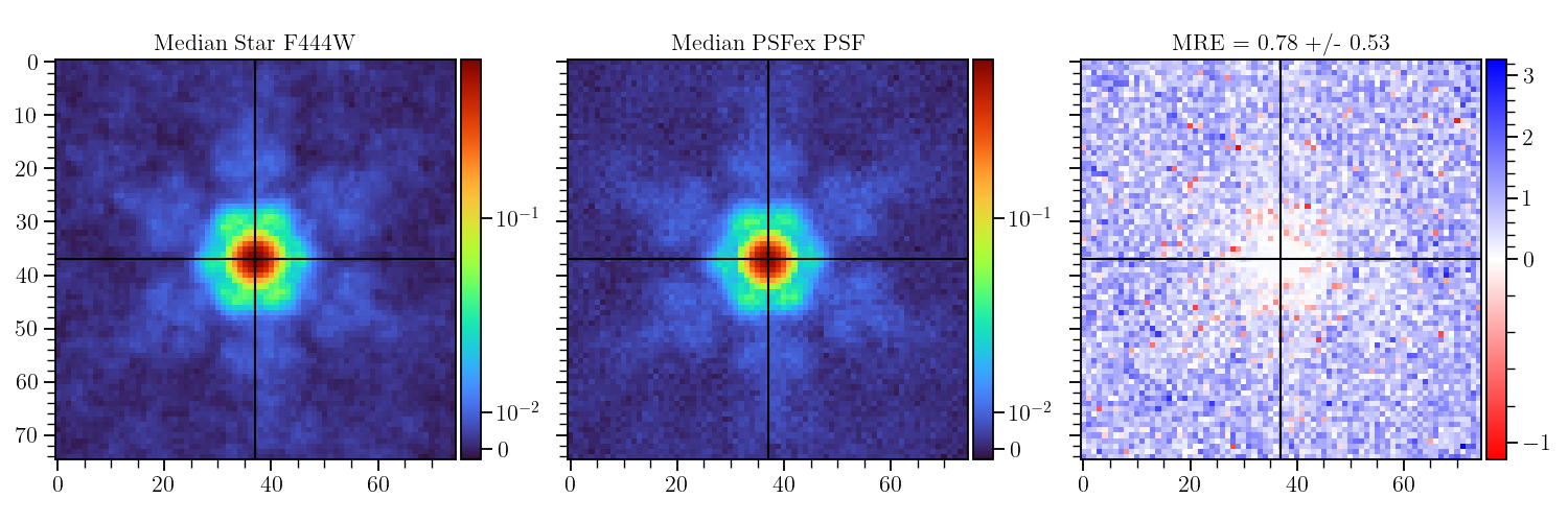
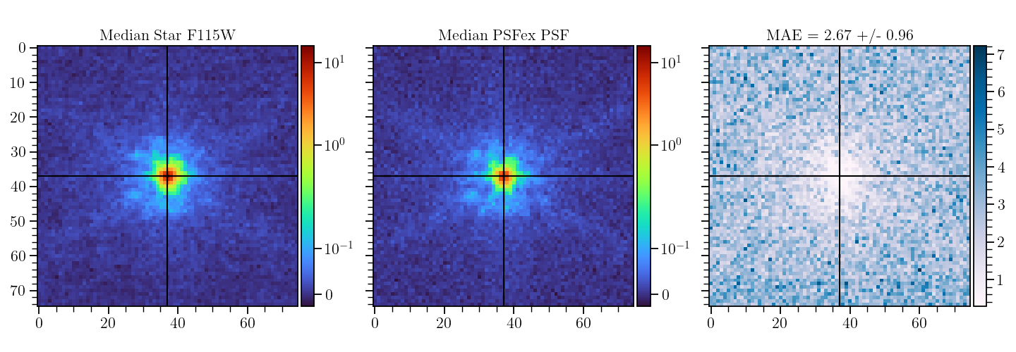
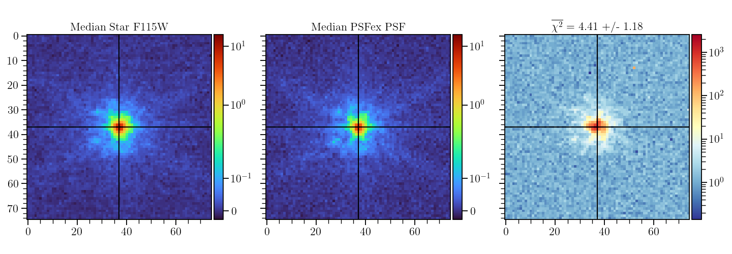
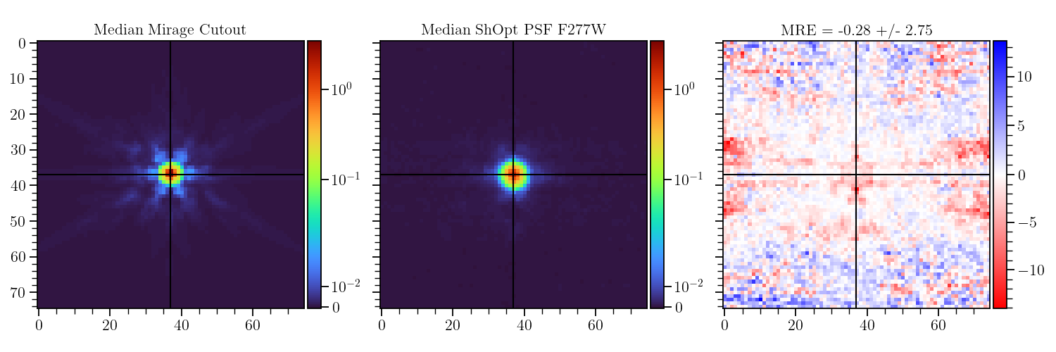
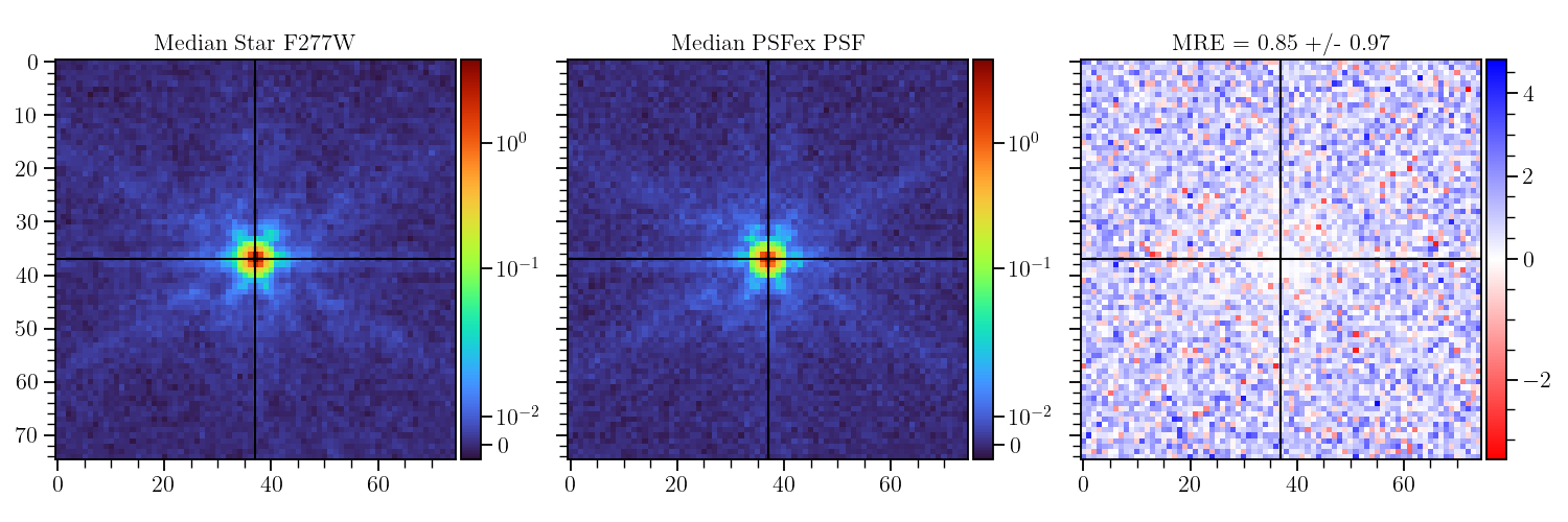
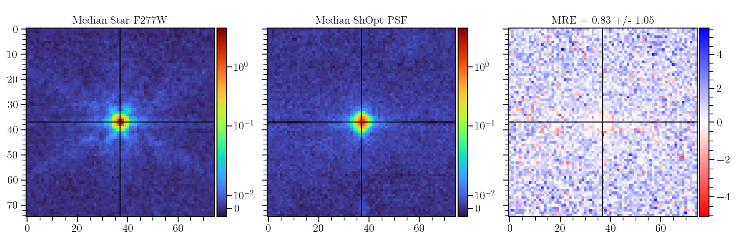
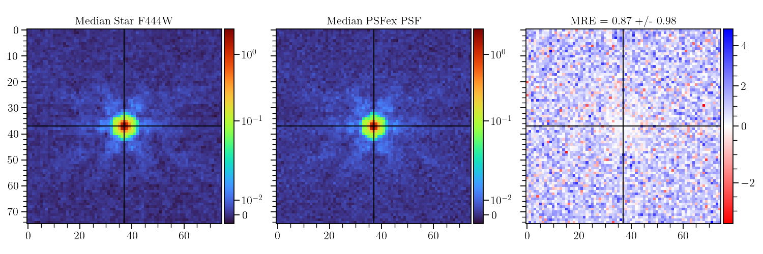
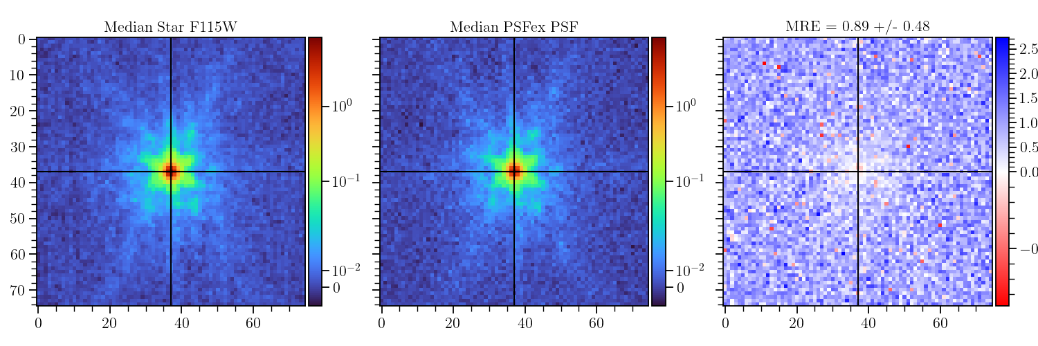
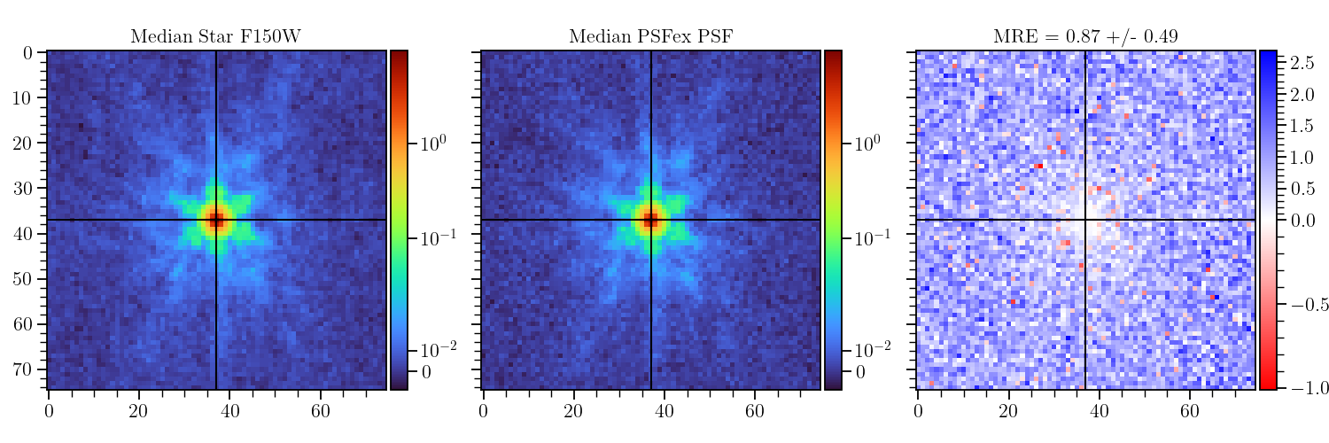
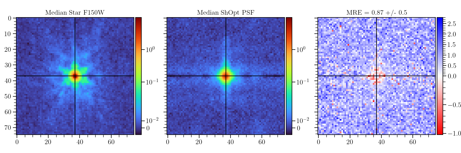
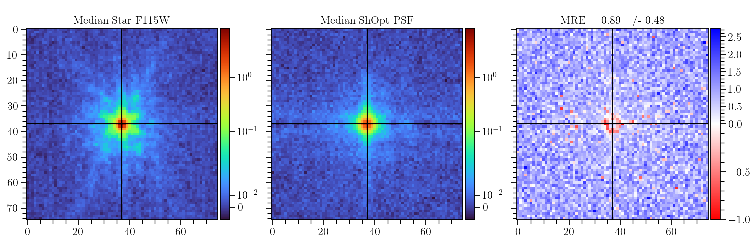
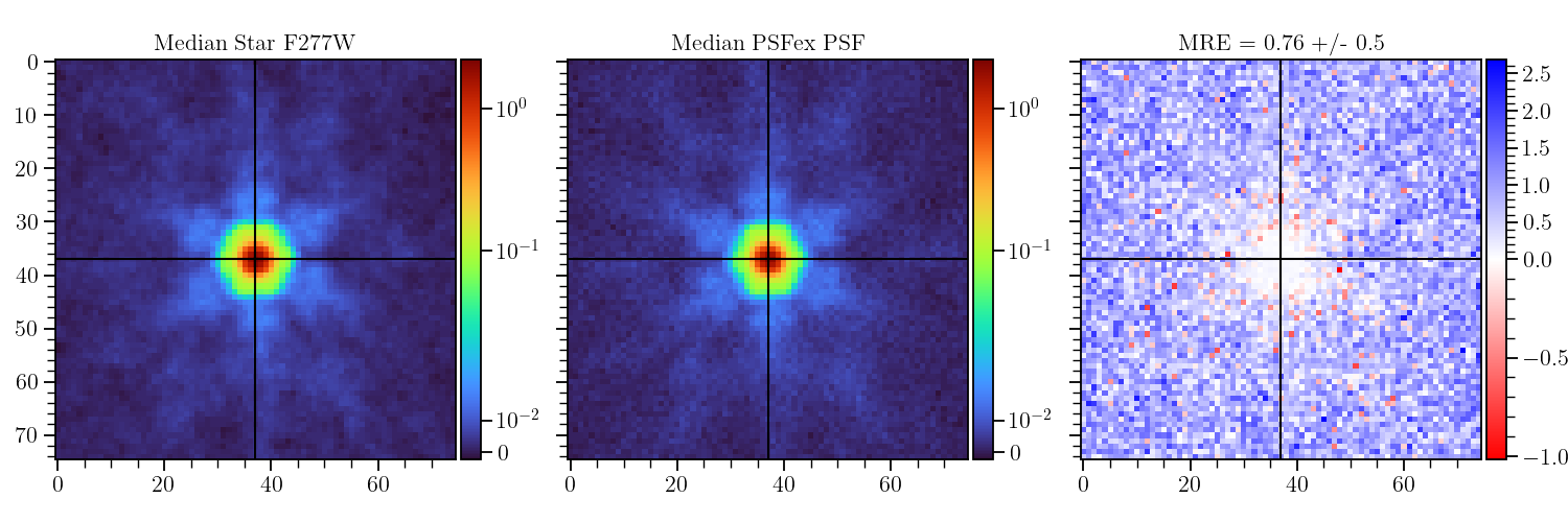
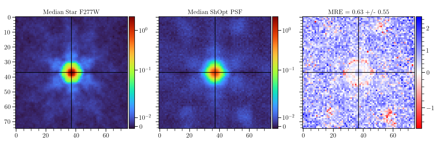
We find similar results for the real data mosaics as for the simulated single exposures, namely that PSFEx produces the most complete models of the PSF structure. Figures 13 and 24-25 suggest that in the main, ShOpt is less successful at modeling the finer details of the PSF, particularly at longer wavelengths.

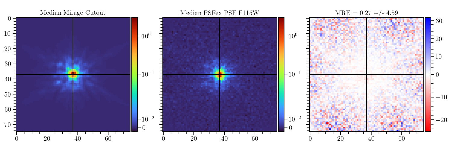
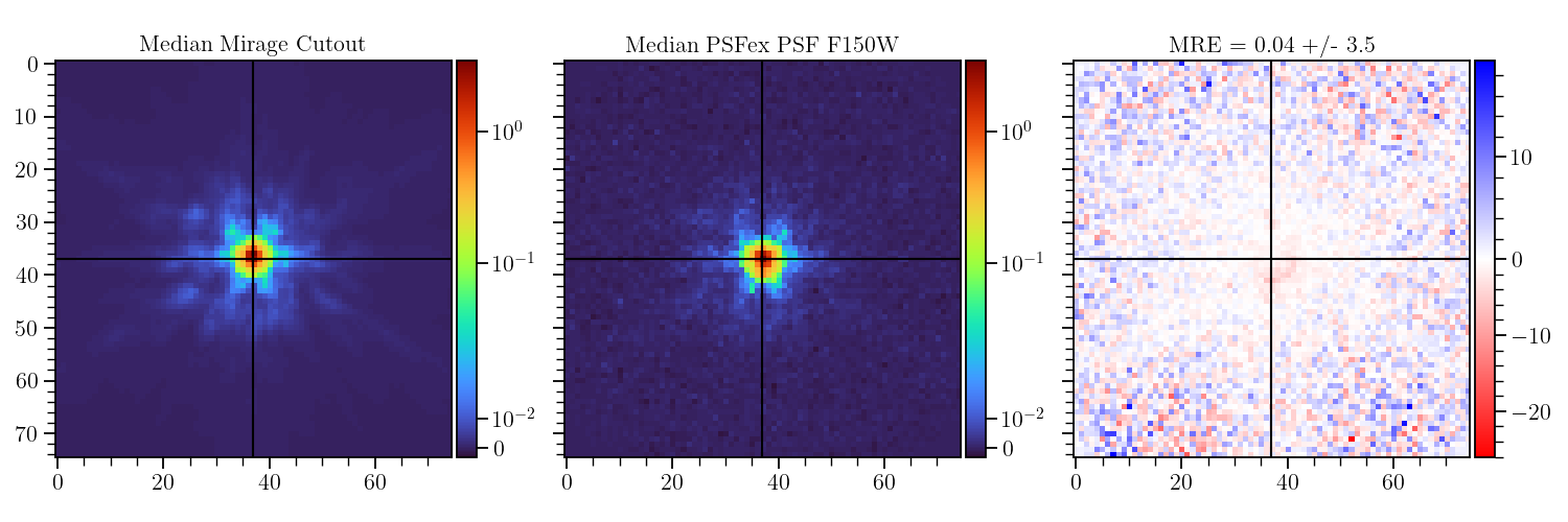
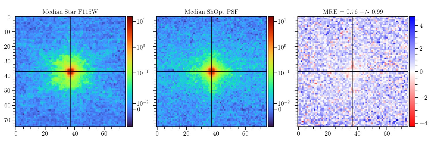
In the short wavelength filters, Figure 24 shows that the PSFEx model captures significantly more detail than the median ShOpt model, which appears featureless. The ShOpt model is also prone to the same over-subtraction in the perimeter of the core of the PSF as seen in the simulated single exposures.

Although the MAE and MRE are consistent between the two fitters, the residual maps shown in Figures 25 and 13 present clear evidence that ShOpt under-performs PSFEx at capturing the details of the PSF core hexagonal structure and outer wings. In these two instances, ShOpt produces PSF models that contain all the requisite structure but are spread out over too large an area.

Figure 13: Evaluation of mean relative error between stars and PSF models for real data mosaics in the F444W bandpass. Left panels show the median star vignette; center panels show the median PSF model; right panels show the mean residuals of individual star-PSF vignettes. Top rows is PSFEx, bottom row is ShOpt.

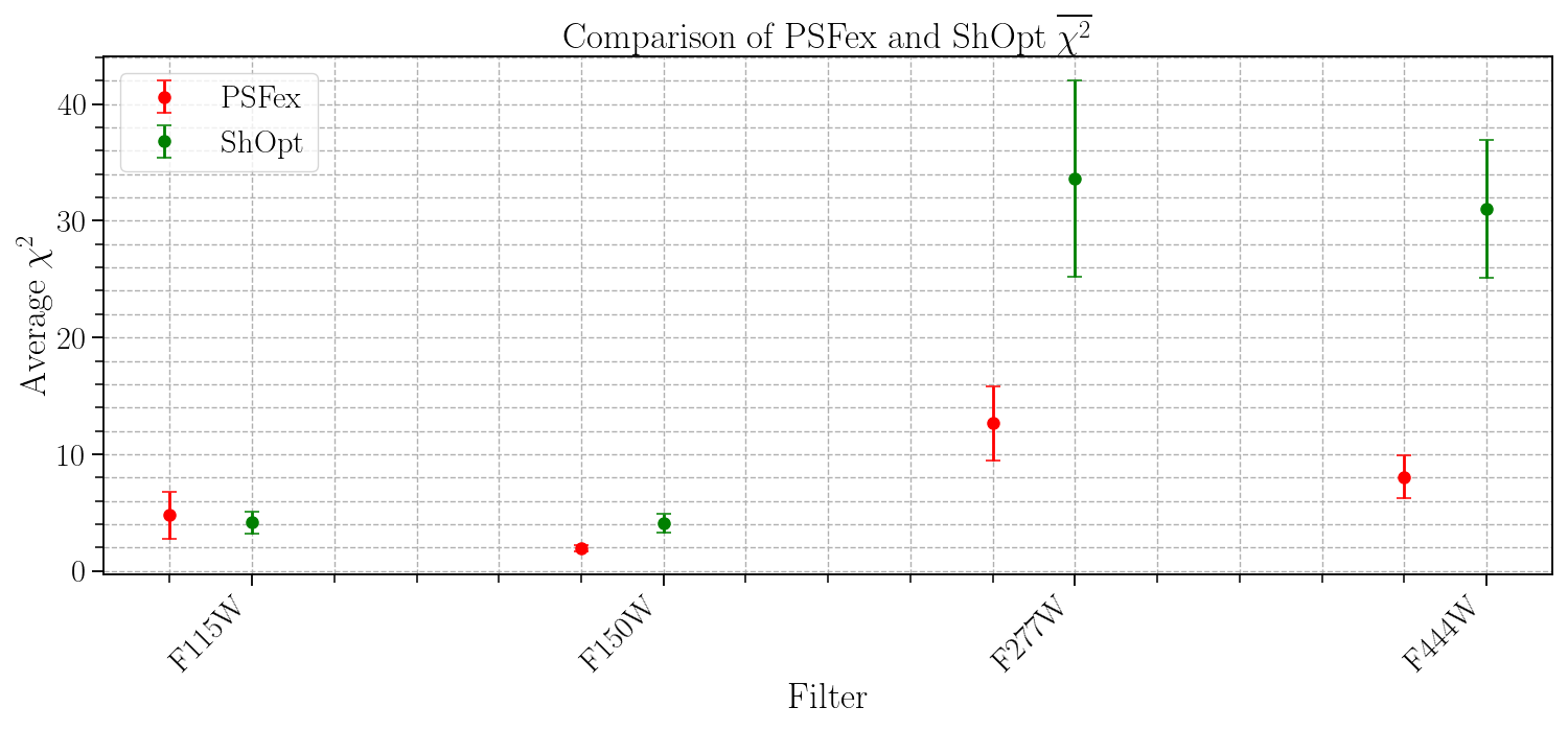
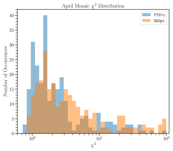
Discrepancy in the performance of PSFEx and ShOpt is further supported by the values of median and mean reduced $\chi^{2}$ in Table 3, as well as the distributions of reduced $\chi^{2}$ in Figures 14 and 15. While at short wavelengths, the reduced $\overline{\chi^{2}}$ values are consistent within error bars, at long wavelengths, the ShOpt $\overline{\chi^{2}}$ differs from PSFEx at the 5 $\sigma$ level. Even if the discrepancy is driven by extreme outliers—as suggested by the long tail of the ShOpt $\chi^{2}$ distribution in Figure 15—the median reduced $\chi^{2}$ values for ShOpt are twice the value of the PSFEx models.

We do not run PIFF on the real mosaics due to timing costs; the real data mosaics cover tens of thousands of pixels, and PIFF fits did not reliably converge.

Figure 14: Confidence of $\overline{\chi^{2}}$ for real data mosaics as a function of bandpass. PSFEx values are shown in red; ShOpt values are shown in green.

Figure 15: Distribution of $\chi^{2}$ for real data mosaics. Not shown are two PSFex $\chi^{2}$ values greater than $100$ and ten ShOpt $\chi^{2}$ values greater than $100$.

Filter	PSF Fitter	MAE	MRE	$\overline{\chi^{2}}$	Median $\chi^{2}$
F115W	ShOpt	2.82$\pm$0.54	0.88$\pm$0.50	3.96$\pm$0.95	1.61
	PSFex	2.76$\pm$0.53	0.90$\pm$0.49	4.49$\pm$2.14	1.45
F150W	ShOpt	2.84$\pm$0.56	0.86$\pm$0.51	2.98$\pm$0.42	1.74
	PSFex	2.77$\pm$0.55	0.87$\pm$0.48	1.64$\pm$0.20	1.26
F277W	ShOpt	2.84$\pm$0.80	0.63$\pm$0.55	36.73$\pm$9.97	6.92
	PSFex	2.56$\pm$0.64	0.75$\pm$0.50	13.55$\pm$3.82	3.49
F444W	ShOpt	2.82$\pm$0.75	0.70$\pm$0.60	27.85$\pm$6.67	4.77
	PSFex	2.59$\pm$0.67	0.78$\pm$0.52	7.36$\pm$2.12	2.45

Table 3: Real mosaic summary statistics.

8.2 Program Speed and Scalability

We investigate how the different PSF fitters handle the simulated mosaic data as the number of pixels in the star vignettes and the degree of the polynomial used to model spatial variations increase. Each PSF fitter is run multiple times to get an average time in seconds for pixel basis fits. For ShOpt, we set the size of the side length $n$ of the analytic fit stamp to be $30$. That is, we use $30\times 30$ pixels to fit the multivariate Gaussian. This is separate from the number of pixels we use for the pixel basis. We do not use any GPU compute power to accelerate the PSF fitters even though ShOpt autoencoder mode can be GPU-accelerated. All of these tests are run on the same hardware using Northeastern’s Discovery Cluster on the zen2 CPUs (Northeastern University Research Computing, 2024). These tests aim to test our calculations in Section 6.

8.2.1 Variation with vignette size

Figure 16: Average execution time as a function of the output size of the PSF sidelength plotted on a log scale.

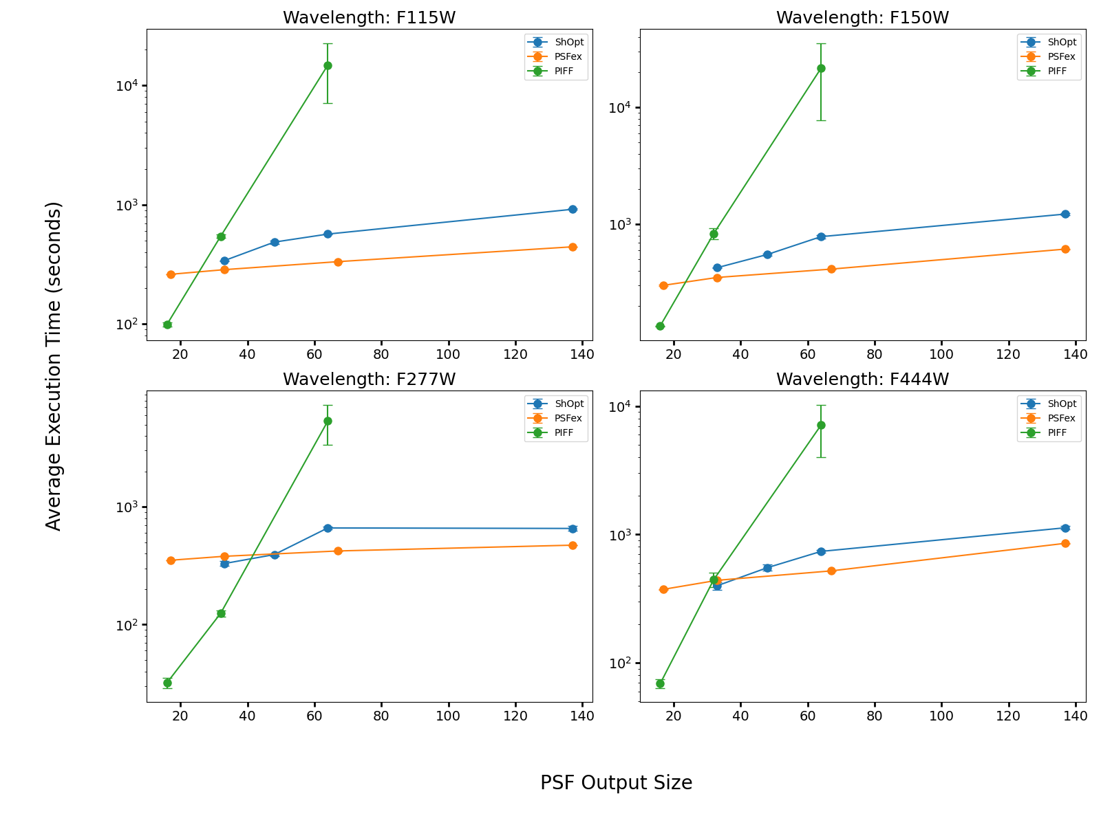
While both ShOpt and PSFEx scale as the output PSF size increases, PIFF does not. For larger PSF sizes, PIFF’s average execution time is an order of magnitude longer than ShOpt or PSFEx. While ShOpt and PSFex required approximately $5$ to $10$ minutes to process PSF sizes of $(137,137)$ for each of the four wavelengths, PIFF consistently took between $1$ and $3$ hours for PSF sizes of $(64,64)$. In the worst case, PIFF can take as much as an entire day to finish. Since PIFF was validated on DECam imaging, which had PSF sizes of $(17,17)$, there was no indication that PIFF tool would not be able to scale. For PSFs of that size, PIFF is actually faster than the other PSF fitters, see Figure 16. While most PSF fitters had consistent completion times, PIFF stood out for $(64,64)$ PSF output sizes, exhibiting greater variability, particularly with shorter wavelengths.

Figure 17: Average execution time as a function of the degree of the interpolating polynomial on $(33,33)$ PSF models plotted on a log scale.

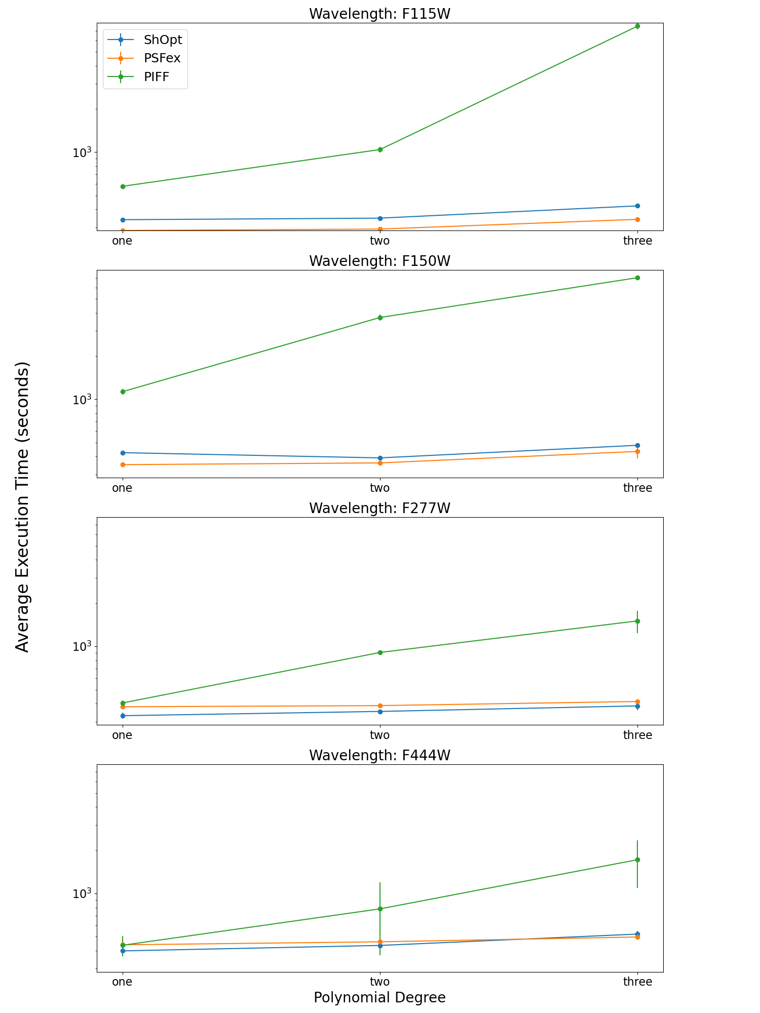
8.2.2 Polynomial Degree

Similarly, while both ShOpt and PSFEx scale as the the degree of the interpolating polynomial increases, PIFF does not. For a degree $1$ interpolation, all three PSF fitters have similar performance for $(33,33)$ PSF sizes. However, as we increase the degree to $2$ and $3$, PIFF takes an order of magnitude longer on average to execution, see Figure 17. For larger degree sizes, PIFF often did not converge to a PSF model with $4\sigma$ confidence after its maximum of $30$ iterations. ShOpt and PSFex maintain a consistent runtime of about $5$ minutes, whereas PIFF experiences a dramatic increase in runtime, going up to hours for short wavelengths with higher degrees of the interpolating polynomial, and by around thirty minutes for longer wavelengths.

9 Discussion and Conclusions

We have presented ShOpt, a new empirical PSF characterization tool, and with it, a methodology for benchmarking the accuracy and computational efficiency of PSF fitting software.

In our assessment of PSF model quality, we produced a series of mean residual images, including normalized mean error, mean absolute error, and chi-squared error. We further condense this information into aggregate statistics that quantify the pixel-level discrepancies between the modeled and actual PSFs across the ensemble of stars being modeled.

Though convenient, we find that single-number figures of merit can mask significant discrepancies between a PSF model and the true PSF. For instance, while a PSFEx model and a ShOpt model might exhibit comparable mean relative errors, the ShOpt model does not fully replicate the complex features of the NIRCam PSF—features which PSFEx managed to capture effectively.

Among the various single-number figures of merit we examined, the average and median chi-squared values were the most indicative of mismatched PSF models. Accordingly, we recommend a holistic approach for evaluating the quality of a particular PSF model, using both aggregate statistics (particularly chi-squared values) and mean residual images.

In Section 6, we predicted that ShOpt’s algorithmic design would allow it to scale as the PSF model size and the degree of the interpolating polynomial increased; this assertion was borne out in our speed testing. Our analysis does not distinguish between the contributions of architectural choices and the Julia language itself to ShOpt’s fast execution time. Regardless, we find that ShOpt delivers speed performance on par with PSFEx, with only marginal differences in processing times for PSF models $(137,137)$ pixels in size (large enough to enclose most of the NIRCam PSF). ShOpt’s competitive speed comes from a combination of multi-threading, imposed geometric constraints, the implementation of the LBFGS algorithm, and a thorough data cleaning pipeline. Conversely, PIFF—optimized for the larger pixel scale of the Dark Energy Camera—does not execute in a reasonable timeframe even for PSF sizes that are $(64,64)$ pixels in size.

The principal limiting factor for accuracy of ShOpt is its iterative refinement process. Although having a fixed iteration count circumvents potential issues with overfitting or non-convergence due to noise artifacts, the specified number of iterations is somewhat arbitrary. Using a dynamic stopping criterion as opposed to a predetermined number of iterations would optimize the refinement process and bolster confidence in the final PSF model.

In its current state, ShOpt  produces an excellent approximation to the NIRCam PSF for simulated mosaics, for which training stars was abundant and outliers were few. Further development will be required to capture the full complexity of the NIRCam PSF, particularly in bandpasses where the PSF is fully sampled and in single exposures, where training stars are more sparse.

Several enhancements are planned for ShOpt that may improve the quality of its PSF models. For example, ShOpt builds models strictly in the native pixel scale of the image; implementing super- or sub-sampling of the image pixel scale would align ShOpt with the standards of other PSF software. A more advanced PCA method for PSF reconstruction, proposed in Lin et al. (2023), is slated for future integration in our PCA mode. Introducing a regularization term to the polynomial interpolation procedure may also curb the tendency to overfit to individual stars. These upgrades, among others, will be featured in future ShOpt releases.

ShOpt incorporates several innovative techniques that could benefit other PSF modeling efforts. These include leveraging manifold properties when fitting analytic profiles; using low-dimensional reconstructions for pixel-basis fits; and pixel-by-pixel parallelization during fitting of spatial variation. Though more work is required for ShOpt to capture the full complexity of the NIRCam PSF, it has nevertheless demonstrated the potential to bridge the speed of PSFEx with the advances of PIFF. We are optimistic that with the algorithmic refinements described above, ShOpt will be able to fully realize its potential as a PSF fitter for next-generation astronomical observatories.

Appendix A Additional PSF Diagnostic Figures

Figure 18: Examples of mean average error (top panel) and $\chi^{2}$ residual figures (bottom panel), shown here for the simulated mosaics in F115W.

Figure 19: Mean relative error between MIRAGE input point source images and PSF models for the F115W and F150W bandpasses. Panels and color bars are the same as Figure 7.

Figure 20: Mean relative error between MIRAGE input point source images and PSF models for the F277W filter. Panels and color bars are the same as Figure 7.

Figure 21: Mean relative error between stars and PSF models for simulated mosaics in the F115W bandpass. Left panels show the median of the vignettes. Panels and color bars are the same as in Figure 10.

Figure 22: Evaluation of mean relative error between stars and PSF models for simulated mosaics in the F277W bandpass. Left panels show the median of the vignettes. Panels and color bars are the same as in Figure 10.

Figure 23: Evaluation of mean relative error between stars and PSF models for simulated mosaics in the F444W bandpass. Left panels show the median of the vignettes. Panels and color bars are the same as in Figure 10.

Figure 24: Mean relative error between stars and PSF models for real data mosaics in the F115W and F150W bandpasses. Color bars are the same as Figure 13.

Figure 25: Evaluation of mean relative error between stars and PSF models for real data mosaics in the F277W bandpass. Panels and color bars are the same as in Figure 13.

Appendix B Running ShOpt

export JULIA_NUM_THREADS=4 # On Windows set JULIA_NUM_THREADS=4 julia shopt.jl [configdir] [outdir] [catalog.fits] See our TutorialNotebook.ipynb or our README.md for more detailed setup instructions on our GitHub.

Appendix C Testing Configs

C.1 Source Extractor config

# Default configuration file for SExtractor 2.25.0
#
#-------------------------------- Catalog ------------------------------------

CATALOG_NAME     catalog.fits  # name of the output catalog
CATALOG_TYPE     FITS_LDAC
PARAMETERS_NAME  sextractor.param  # name of the file containing catalog contents

#------------------------------- Extraction ----------------------------------

DETECT_TYPE      CCD            # CCD (linear) or PHOTO (with gamma correction)
DETECT_MINAREA   8              # min. # of pixels above threshold
DETECT_MAXAREA   0              # max. # of pixels above threshold (0=unlimited)
THRESH_TYPE      RELATIVE       # threshold type: RELATIVE (in sigmas)
                                # or ABSOLUTE (in ADUs)
DETECT_THRESH    2             # <sigmas> or <threshold>,<ZP> in mag.arcsec-2
ANALYSIS_THRESH  2            # <sigmas> or <threshold>,<ZP> in mag.arcsec-2

FILTER           Y              # apply filter for detection (Y or N)?
FILTER_NAME  gauss_2.5_5x5.conv # name of the file containing the filter
FILTER_THRESH                   # Threshold[s] for retina filtering

DEBLEND_NTHRESH  32             # Number of deblending sub-thresholds
DEBLEND_MINCONT  0.005          # Minimum contrast parameter for deblending
CLEAN            Y              # Clean spurious detections? (Y or N)?
CLEAN_PARAM      1.0            # Cleaning efficiency

MASK_TYPE        CORRECT        # type of detection MASKing: can be one of
                                # NONE, BLANK or CORRECT

#-------------------------------- WEIGHTing ----------------------------------

WEIGHT_TYPE    MAP_WEIGHT       # type of WEIGHTing: NONE, BACKGROUND,
                                # MAP_RMS, MAP_VAR or MAP_WEIGHT
RESCALE_WEIGHTS  Y              # Rescale input weights/variances (Y/N)?
WEIGHT_IMAGE     weight.fits    # weight-map filename
WEIGHT_GAIN      Y              # modulate gain (E/ADU) with weights? (Y/N)
WEIGHT_THRESH    0              # weight threshold[s] for bad pixels

#-------------------------------- FLAGging -----------------------------------

FLAG_IMAGE       flag.fits      # filename for an input FLAG-image
FLAG_TYPE        OR             # flag pixel combination: OR, AND, MIN, MAX
                                # or MOST

#----------------------- Differential Geometry Map ---------------------------

DGEO_TYPE        NONE           # Differential geometry map type: NONE or PIXEL
DGEO_IMAGE       dgeo.fits      # Filename for input differential geometry image

#------------------------------ Photometry -----------------------------------

PHOT_APERTURES   31            # MAG_APER aperture diameter(s) in pixels
PHOT_AUTOPARAMS  2, 2.5         # MAG_AUTO parameters: <Kron_fact>,<min_radius>
PHOT_PETROPARAMS 2.0, 3.5       # MAG_PETRO parameters: <Petrosian_fact>,
                                # <min_radius>
PHOT_AUTOAPERS   0.0,0.0        # <estimation>,<measurement> minimum apertures
                                # for MAG_AUTO and MAG_PETRO
PHOT_FLUXFRAC    0.5            # flux fraction[s] used for FLUX_RADIUS

SATUR_LEVEL      37000.0        # level (in ADUs) at which arises saturation
SATUR_KEY        SATURATE       # keyword for saturation level (in ADUs)

MAG_ZEROPOINT    28.086519392           # magnitude zero-point
MAG_GAMMA        4.0            # gamma of emulsion (for photographic scans)
GAIN             0.0            # detector gain in e-/ADU
GAIN_KEY         GAIN           # keyword for detector gain in e-/ADU
PIXEL_SCALE      0              # size of pixel in arcsec (0=use FITS WCS info)

#------------------------- Star/Galaxy Separation ----------------------------

SEEING_FWHM      0.07           # stellar FWHM in arcsec
STARNNW_NAME     default.nnw    # Neural-Network_Weight table filename

#------------------------------ Background -----------------------------------

BACK_TYPE        AUTO           # AUTO or MANUAL
BACK_VALUE       0.0            # Default background value in MANUAL mode
BACK_SIZE        128            # Background mesh: <size> or <width>,<height>
BACK_FILTERSIZE  3              # Background filter: <size> or <width>,<height>

BACKPHOTO_TYPE   LOCAL          # can be GLOBAL or LOCAL
BACKPHOTO_THICK  24             # thickness of the background LOCAL annulus
BACK_FILTTHRESH  0.0            # Threshold above which the background-
                                # map filter operates

#------------------------------ Check Image ----------------------------------

CHECKIMAGE_TYPE  -BACKGROUND,APERTURES  # can be NONE, BACKGROUND, BACKGROUND_RMS,
                                # MINIBACKGROUND, MINIBACK_RMS, -BACKGROUND,
                                # FILTERED, OBJECTS, -OBJECTS, SEGMENTATION,
                                # or APERTURES
CHECKIMAGE_NAME  im.sub.fits,im.aper.fits  # Filename for the check-image

#--------------------- Memory (change with caution!) -------------------------

MEMORY_OBJSTACK  5000           # number of objects in stack
MEMORY_PIXSTACK  500000         # number of pixels in stack
MEMORY_BUFSIZE   4096           # number of lines in buffer

#------------------------------- ASSOCiation ---------------------------------

ASSOC_NAME       sky.list       # name of the ASCII file to ASSOCiate
ASSOC_DATA       2,3,4          # columns of the data to replicate (0=all)
ASSOC_PARAMS     2,3,4          # columns of xpos,ypos[,mag]
ASSOCCOORD_TYPE  PIXEL          # ASSOC coordinates: PIXEL or WORLD
ASSOC_RADIUS     2.0            # cross-matching radius (pixels)
ASSOC_TYPE       NEAREST        # ASSOCiation method: FIRST, NEAREST, MEAN,
                                # MAG_MEAN, SUM, MAG_SUM, MIN or MAX
ASSOCSELEC_TYPE  MATCHED        # ASSOC selection type: ALL, MATCHED or -MATCHED

#----------------------------- Miscellaneous ---------------------------------

VERBOSE_TYPE     NORMAL         # can be QUIET, NORMAL or FULL
HEADER_SUFFIX    .head          # Filename extension for additional headers
WRITE_XML        N              # Write XML file (Y/N)?
XML_NAME         sex.xml        # Filename for XML output
XSL_URL          file:///anaconda2/envs/py3/share/sextractor/sextractor.xsl
                                # Filename for XSL style-sheet
NTHREADS         1              # 1 single thread

FITS_UNSIGNED    N              # Treat FITS integer values as unsigned (Y/N)?
INTERP_MAXXLAG   16             # Max. lag along X for 0-weight interpolation
INTERP_MAXYLAG   16             # Max. lag along Y for 0-weight interpolation
INTERP_TYPE      ALL            # Interpolation type: NONE, VAR_ONLY or ALL

#--------------------------- Experimental Stuff ---------------------------F--

PSF_NAME         default.psf    # File containing the PSF model
PSF_NMAX         1              # Max.number of PSFs fitted simultaneously
PATTERN_TYPE     RINGS-HARMONIC # can RINGS-QUADPOLE, RINGS-OCTOPOLE,
                                # RINGS-HARMONICS or GAUSS-LAGUERRE
SOM_NAME         default.som    # File containing Self-Organizing Map weights

C.2 ShOpt config

saveYaml: true #save this file with each run

mode: "PCA" # Options: auotoencoder, PCA. Make sure mode is a string with double quotes

PCAterms: 50 #If PCA mode is enabled, how many moments do you want to use for your pixel grid fit

lanczos: 5 #The size of the smoothing kernel

NNparams: #For if Autoencoder mode is enabled
  epochs: 100 # max number of training epochs for each pixel grid fit
  minGradientPixel: 1e-5 # the stopping gradient of the loss function for the pixel grid fit

AnalyticFitParams: # for fitting analytic profile
  minGradientAnalyticModel: 1e-6 #stopping gradient for LBFGS on vignettes
  minGradientAnalyticLearned: 1e-6 #stopping gradient for LBFGS on pixel grid models
  analyticFitStampSize: 64 #the subset of pixels you wish to fit the analytic profile to

dataProcessing:
  SnRPercentile: 0.33 #Filter this % of stars based off of signal to noise
  sUpperBound: 1 #Filter stars based off of this s value found by analytic profile fits as an upper bound
  sLowerBound: 0.075 #Filter stars based off of this s value found by analytic profile fits as a lower bound

plots: #What plots do you want?
  unicodePlots: true
  normalPlots:
    parametersHistogram: true
    parametersScatterplot: true
  cairomakiePlots:
    streamplots: false
  pythonPlots: false

polynomialDegree: 1 #degree of polynomial for interpolation
stampSize: 130 #how many pixels should the pixel grid PSF model

training_ratio: 0.9 #how many stars are you using the train versus to validate the PSF fit
sum_pixel_grid_and_inputs_to_unity: false #Sum flux to unity true or false

polynomial_interpolation_stopping_gradient: 1e-12 #stopping gradient for LFBGS used for polynomial interpolation

summary_name: ’’ #name to prefix summary.shopt
truncate_summary_file: true # do you want to save storage by only storing essential information, how to reconstruct the PSF and analytic models

CommentsOnRun: "** This is where you can leave comments or notes to self on the run! **"

C.3 PIFF config

# modules and input.wcs fields, in which case, the code will use the (less
# accurate) WCS that ships with the image in the fits file.

input:

    # Input file directory
    dir: "./"

    # You can specify this either as a single filenames, a list of
    # filenames, or something that glob.glob() will understand.
    image_file_name: ’round1/mock_superbit_obs_001.sub.fits’

    image_hdu: 1    # When rice-compressed, image is in hdu=1, not hdu=0.
    weight_hdu: 4

    cat_file_name: ’round1/mock_superbit_obs_001_stars.ldac’

    cat_hdu: 2

    # We use the GalSim config parser, which lets you eval python lines by starting a
    # string with $.
    # You can also grab the current value of some other item in the config during processing.
    # In this case input.image_file_name is the current image file name.
    # Then this strips off the ending, starting with ’_’, gets the bit before the ’.’, and
    # converts it to an integer.
    # chipnum: "$int((@input.image_file_name).rsplit(’_’)[-3][1:])"

    # What columns in the catalog have things we need?
    x_col: XWIN_IMAGE
    y_col: YWIN_IMAGE
    ra_col: ALPHAWIN_J2000
    dec_col: DELTAWIN_J2000

    # The telescope pointing is in the image header
    ra: 149.9303551903936
    dec: 2.380272767453749

    # DES Y3 processed images are normalized to have gain=1.
    # Leave blank if you don’t know what it is!
    # gain: 1

    # How large should the postage stamp cutouts of the stars be?
    stamp_size: 100

    # Use all cores for reading the input files
    nproc: -1

    # Tell Piff to use the better Pixmappy WCS, not the one in the FITS file.
    # If you don’t want to install Pixmappy, you can just comment out this bit and the
    # modules section above, and it will just use the WCS in the FITS file rather than this.
    #wcs:
    #    type: Pixmappy
    #    dir: "350139"
    #    # Note: This file was modified to only include the parts relevant to this exposure.
    #    # DES users would normally just use the full zone135.astro file.
    #    file_name: ’zone135_mod.astro’
    #    exp: 350139
    #    ccdnum: ’@input.chipnum’

select:

    # For bright stars, weight them equivalent to snr=100 stars, not higher.
    max_snr: 100

    # Remove stars with snr < 10
    min_snr:  10

    # Reserve 15% of the stars for diagnostics
    reserve_frac: 0.15

    hsm_size_reject: True

    # If you want the reserve choice consistent across runs, set this to something.
    seed:

psf:

    # This type of PSF will use a separate model/interp solution for each chip.
    # But all the solutions will be given in a single output file.
    # For the DES Y3 solutions, we actually did type: Simple, which is almost the
    # same, but makes a separate file for each CCD.
    type: SingleChip

    # Also use all cores when finding psf
    nproc: -1

    outliers:


        type: Chisq

        # The threshold is given in terms of nsigma equivalent, since that’s how we normally
        # think of this, but really this is based on the chisq probability distribution for the
        # number of degrees of freedom the model has.
        nsigma: 4

        # Only remove at most 1% of the stars per iteration.
        # Can also set this to an integer to remove at most that many.
        max_remove: 0.03

    model:

        # This model uses a grid of pixels to model the surface brightness distribution.
        type: PixelGrid
        scale: 0.03      # NIRCam ative pixel scale
        size: 75         # Model is 24 x 24 in these pixels

    interp:

        # This interpolator does some of the model solving when interpolating to handle degenerate
        # information from masking and the fact that the pixels are smaller than native.
        type: BasisPolynomial
        order: 1

output:

    # Give the name of the output file.  It’s a fits file, but it doesn’t need to end in .fits.
    dir: piff-output
    file_name: "psf_model.piff"

    # You may also output a number of stats outputs.
    stats:
        -
            # This produces an output catalog with the mesured sizes, shapes of the stars and
            # the PSF models.  Reserve stars are marked as such in a reserve column.
            type: HSMCatalog
            file_name: "piff_cat.fits"

        -
            # The rest of these are all plots of various statistics about the residuals.
            # This one shows histograms of the size and shape residuals
            type: ShapeHist
            file_name: "piff_shapes.png"
            cut_frac: 0.03   # Default cuts off 1% from each side.
                             # This mostly excludes some outliers we don’t much care about.
                             # There are enough stars here that we can reduce this a bit to show
                             # more of the wings.

        -
            # These are the classic rho stats.  They are pretty noisy for just a single
            # exposure, but they can check for egregious errors.
            type: Rho
            file_name: "piff_rho.png"
            # These parameters are TreeCorr parameters for doing the correlation functions.
            min_sep: 0.3
            max_sep: 12
            sep_units: arcmin
            bin_size: 0.4

        -
            # This bins the residuals across the field of view.
            type: TwoDHist
            file_name: "piff_twod.png"
            nbins_u: 15  # Default is 20 for these, but the FOV is large enough that 50 looks good.
            nbins_v: 15

        -
            # This makes a whisker plot of both the raw PSF shape and the PSF shape residuals
            # across the field of view.
            type: Whisker
            file_name: "piff_whisker.png"

        -
            # This selects 20 (nplot) random stars and shows images of the data, the model,
            # and the residual.  When fits are behaving badly, this can give useful clues
            # about the nature of the problem.
            type: Star
            file_name: "piff_stars.png"
            nplot: 20  # Default is 10.  0 will show all the stars, which would be a lot here.

        -
            # Size-magnitude plots?!
            type: SizeMag
            file_name: "piff_sizemag.png"


# Set the verbosity level a little higher than default (1) to give extra information
# about the progress.
verbose: 2

C.4 PSFex Config

# Default configuration file for PSFEx 3.17.1
# EB 2016-06-28
#

#-------------------------------- PSF model ----------------------------------

BASIS_TYPE      PIXEL           # NONE, PIXEL, GAUSS-LAGUERRE or FILE
#BASIS_NUMBER   30              # Basis number or parameter
PSF_SAMPLING    0               # Sampling step in pixel units (0.0 = auto)
PSF_SIZE        261             # Image size of the PSF model
PSF_RECENTER    Y
#------------------------- Point source measurements -------------------------

CENTER_KEYS     XWIN_IMAGE,YWIN_IMAGE # Catalogue parameters for source pre-centering
PHOTFLUX_KEY    FLUX_APER(1)    # Catalogue parameter for photometric norm.
PHOTFLUXERR_KEY FLUXERR_APER(1) # Catalogue parameter for photometric error

#----------------------------- PSF variability -------------------------------

PSFVAR_KEYS     XWIN_IMAGE,YWIN_IMAGE # Catalogue or FITS (preceded by :) params
PSFVAR_GROUPS   1,1             # Group tag for each context key
PSFVAR_DEGREES  1               # Polynom degree for each group

#----------------------------- Sample selection ------------------------------

SAMPLE_AUTOSELECT  Y           # Automatically select the FWHM (Y/N) ?
SAMPLEVAR_TYPE    NONE         # File-to-file PSF variability: NONE or SEEING
SAMPLE_FWHMRANGE   1,20        # Allowed FWHM range (2.7,3.2)
SAMPLE_VARIABILITY 0.3         # Allowed FWHM variability (1.0 = 100%)
SAMPLE_MINSN       50         # Minimum S/N for a source to be used
SAMPLE_MAXELLIP    0.3         # Maximum (A-B)/(A+B) for a source to be used

#----------------------------- Output catalogs -------------------------------

OUTCAT_TYPE        FITS_LDAC      # NONE, ASCII_HEAD, ASCII, FITS_LDAC
OUTCAT_NAME        psfex_out.cat  # Output catalog filename


#------------------------------- Check-plots ----------------------------------

CHECKPLOT_DEV       PDF         # NULL, XWIN, TK, PS, PSC, XFIG, PNG,
                                # JPEG, AQT, PDF or SVG
CHECKPLOT_RES       0           # Check-plot resolution (0 = default)
CHECKPLOT_ANTIALIAS Y           # Anti-aliasing using convert (Y/N) ?
CHECKPLOT_TYPE      NONE #SELECTION_FWHM,FWHM,ELLIPTICITY,COUNTS,COUNT_FRACTION,CHI2,RESIDUALS
                                # or NONE
CHECKPLOT_NAME      selfwhm,fwhm,ellipticity,counts,countfrac,chi2,resi


#------------------------------ Check-Images ---------------------------------

CHECKIMAGE_TYPE CHI,SAMPLES,RESIDUALS,SNAPSHOTS, -SYMMETRICAL
                                # or MOFFAT,-MOFFAT,-SYMMETRICAL
CHECKIMAGE_NAME chi.fits,samp.fits,resi.fits,snap.fits, minus_symm.fits
                                # Check-image filenames
CHECKIMAGE_CUBE Y

#----------------------------- Miscellaneous ---------------------------------

PSF_DIR                         # Where to write PSFs (empty=same as input)
VERBOSE_TYPE    FULL            # can be QUIET,NORMAL,LOG or FULL
WRITE_XML       Y               # Write XML file (Y/N)?
XML_NAME        psfex.xml       # Filename for XML output
NTHREADS        0               # Number of simultaneous threads for
                                # the SMP version of PSFEx
                                # 0 = automatic

C.5 Shell Script

This is given to inform how much memory we requested from Discovery for purposes of speed testing.

#!/bin/bash
#SBATCH --nodes=1
#SBATCH --mem=16G
#SBATCH --cpus-per-task=4
#SBATCH --time=24:00:00
#SBATCH --partition=short
#SBATCH --job-name=150_A6
#SBATCH --ntasks=1
#SBATCH --constraint=zen2            # Requesting specific CPU architecture
pwd
source /work/mccleary_group/berman.ed/minicondaInstall/bin/activate
python get_jwst_psf.py -config configs/box_cutter.yaml file #file is a placeholder for a fits file

Appendix D Additional ShOpt Checkplots and Outputs

D.1 Diagnostic Material

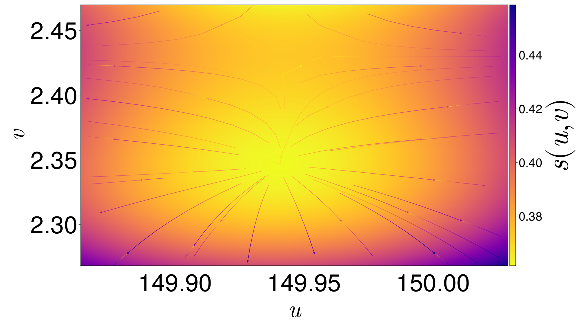
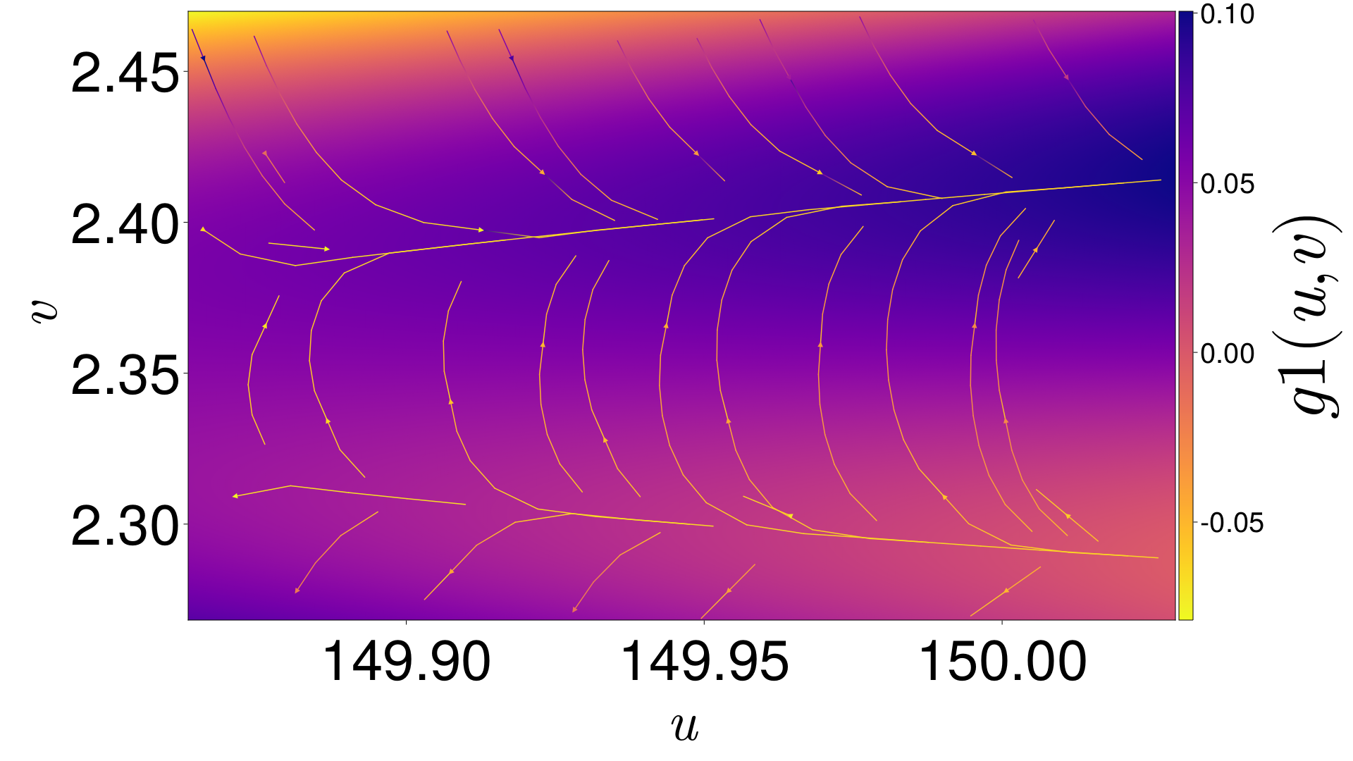
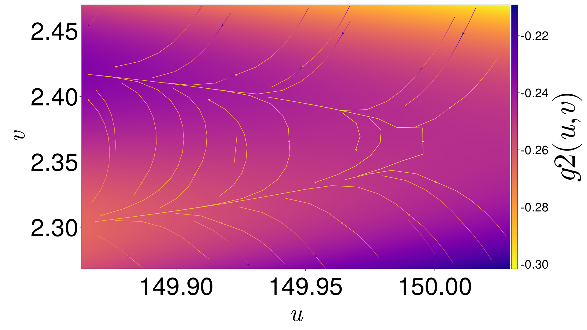
ShOpt provides the following streamplots (Figure 26) to give the user an inclination toward how the PSF is changing across the field of view. We also have a Julia script, reader.jl that reads in the summary.shopt file and provides easy PSF reconstruction. If you want to do your analysis in Python, we also have Python code available for reading in summary.shopt files here https://github.com/EdwardBerman/sigma-Eta-Shopt-Reader.

D.2 summary.shopt

summary.shopt contains $6$ relevant extensions. The first extension is named polynomial matrix, and it contains a $3-$dimension matrix. $2-$dimensions correspond to the dimensions of the input vignettes and the third dimension corresponds to the coefficients of the polynomial at that pixel. The second extension contains all data relevant to learned parameters $\left[s,g_{1},g_{2}\right]$ as well as the $(u,v)$ coordinates at each star. We also measure the mean relative error between stars and their pixel grid fits before the polynomial interpolation step. Note that only stars that make it through all filters are contained. The third, and fourth extensions contain $3-$dimensional arrays corresponding to the input vignettes and the pixel grid fits of the vignettes. The fifth extension provides flags that tell you the indices of stars that were filtered out of the final interpolation step. The sixth extension tells you how to find $\left[s,g_{1},g_{2}\right]$ at an arbitrary $(u,v)$. There is also a mode that only outputs the first, second, and sixth extensions for reasons related to storage concern. This is enabled by default.

(a) $s(u,v)$

(b) $g_{1}(u,v)$

(c) $g_{2}(u,v)$

Figure 26: Stream plots demonstrating how variables $\left[s,g_{1},g_{2}\right]$ vary across the field of view (in astrometric coordinates $(u,v)$) for the F115W simulated mosaic image. Recall that $s$ corresponds to size and $g_{1},g_{2}$ correspond to shear.

D.3 Command Line Outputs

As an extra convenience, we give users the option to display some of the diagnostic material to the terminal using UnicodePlots.jl. This may be useful for less scrupulous more exploratory runs of our software or for users looking for a quick sanity check that everything ran correctly without having to navigate to an output directory and open all of the saved checkplots.

We also print out to the terminal some key information about what is happening as the program runs, including what the program is doing, how many and which stars are failing or being filtered, progress on fitting, and how long particular portions of the code took to run.

Appendix E Petal Diagrams

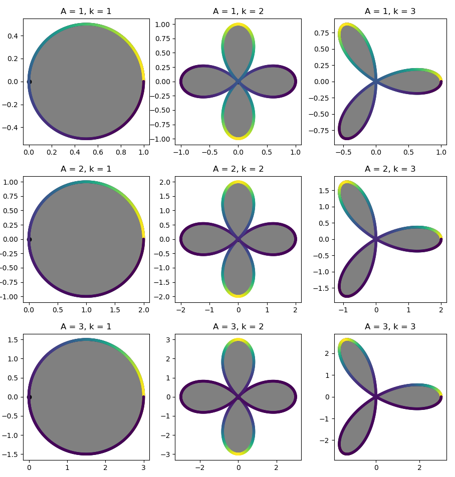
We speculate that petal diagrams may be able to approximate the spiky natures of JWST PSFS. Consider $r=A\cos(k\theta+\gamma)$, shown below in Figure 27 for different $\left[A,k\right]$ values where $\gamma=0$. In practice, $\left[A,k,\gamma\right]$ could be learnable parameters. We could then choose some $f(r)\propto\frac{1}{r}$ such that the gray fades from black to white. We would define $f(r)$ piecewise such that it is $0$ outside of the petal and decreases radially with $r$ inside the petal. The upshot of this approach is that we can just look at the learned $k$ and immediately know if our PSF captures the correct number of wings. Alternatively, Bergé et al. (2019) introduced exponential shapelets with an orthogonal separation of $r$ and $\theta$, that may also be useful.

Figure 27: Petal diagrams approximating different PSFs. Different k values correspond to PSF with different numbers of spikes. The A value determines how long the spikes are. Here, all of the pixels inside the petals (gray) are set to a constant value, and everything outside is $0$.

References

- Absil et al. (2008) Absil, P.-A., Mahony, R., & Sepulchre, R. 2008, Optimization Algorithms on Matrix Manifolds (Princeton, NJ: Princeton University Press), xvi+224
- Bagley et al. (2022) Bagley, M. B., Finkelstein, S. L., Rojas-Ruiz, S., et al. 2022, arXiv e-prints, arXiv:2205.12980, doi: 10.48550/arXiv.2205.12980
- Beichman et al. (2012) Beichman, C. A., Rieke, M., Eisenstein, D., et al. 2012, in Society of Photo-Optical Instrumentation Engineers (SPIE) Conference Series, Vol. 8442, Space Telescopes and Instrumentation 2012: Optical, Infrared, and Millimeter Wave, ed. M. C. Clampin, G. G. Fazio, H. A. MacEwen, & J. Oschmann, Jacobus M., 84422N, doi: 10.1117/12.925447
- Bergé et al. (2019) Bergé, J., Massey, R., Baghi, Q., & Touboul, P. 2019, Monthly Notices of the Royal Astronomical Society, 486, 544
- Bergmann (2022) Bergmann, R. 2022, Journal of Open Source Software, 7, 3866, doi: 10.21105/joss.03866
- Berman & McCleary (2023) Berman, E., & McCleary, J. 2023, ShOpt.jl: A Julia Package for Empirical Point Spread Function Characterization of JWST NIRCam Data. https://arxiv.org/abs/2310.00071
- Bernstein & Jarvis (2002) Bernstein, G. M., & Jarvis, M. 2002, The Astronomical Journal, 123, 583, doi: 10.1086/338085
- Bertin (2011) Bertin, E. 2011, in Astronomical Society of the Pacific Conference Series, Vol. 442, Astronomical Data Analysis Software and Systems XX, ed. I. N. Evans, A. Accomazzi, D. J. Mink, & A. H. Rots, 435
- Bertin & Arnouts (1996) Bertin, E., & Arnouts, S. 1996, A&AS, 117, 393, doi: 10.1051/aas:1996164
- Boumal (2023) Boumal, N. 2023, An introduction to optimization on smooth manifolds (Cambridge University Press), doi: 10.1017/9781009166164
- Bushouse et al. (2023) Bushouse, H., Eisenhamer, J., Dencheva, N., et al. 2023, JWST Calibration Pipeline, 1.13.1, doi: 10.5281/zenodo.7038885
- Casey et al. (2023) Casey, C. M., Kartaltepe, J. S., Drakos, N. E., et al. 2023, COSMOS-Web: An Overview of the JWST Cosmic Origins Survey. https://arxiv.org/abs/2211.07865
- Cassano et al. (2023) Cassano, F., Gouwar, J., Lucchetti, F., et al. 2023, Knowledge Transfer from High-Resource to Low-Resource Programming Languages for Code LLMs. https://arxiv.org/abs/2308.09895
- Finkelstein et al. (2022) Finkelstein, S. L., Bagley, M. B., Arrabal Haro, P., et al. 2022, ApJ, 940, L55, doi: 10.3847/2041-8213/ac966e
- Fu et al. (2022) Fu, S., Dell’Antonio, I., Chary, R.-R., et al. 2022, The Astrophysical Journal, 933, 84, doi: 10.3847/1538-4357/ac68e8
- Hilbert et al. (2019) Hilbert, B., Sahlmann, J., Volk, K., et al. 2019, spacetelescope/mirage: First github release, v1.1.1, Zenodo, Zenodo, doi: 10.5281/zenodo.3519262
- Innes (2018) Innes, M. 2018, Journal of Open Source Software, doi: 10.21105/joss.00602
- Jarvis et al. (2020) Jarvis, M., Bernstein, G. M., Amon, A., et al. 2020, Monthly Notices of the Royal Astronomical Society, 501, 1282, doi: 10.1093/mnras/staa3679
- Ji et al. (2023) Ji, Z., Williams, C. C., Tacchella, S., et al. 2023, arXiv preprint arXiv:2305.18518
- Kokorev et al. (2021) Kokorev, V. I., Magdis, G. E., Davidzon, I., et al. 2021, ApJ, 921, 40, doi: 10.3847/1538-4357/ac18ce
- Krist et al. (2011) Krist, J. E., Hook, R. N., & Stoehr, F. 2011, in Optical Modeling and Performance Predictions V, Vol. 8127, SPIE, 166–181
- Kung et al. (2021) Kung, H., Natesh, V., & Sabot, A. 2021, in SC21: International Conference for High Performance Computing, Networking, Storage and Analysis, 1–13, doi: 10.1145/3458817.3476166
- Lin et al. (2023) Lin, Nie, Huanyuan, et al. 2023, HybPSF: Hybrid PSF reconstruction for the observed JWST NIRCam image. https://arxiv.org/abs/2308.14065
- Maas (2013) Maas, A. L. 2013, in ICML. https://api.semanticscholar.org/CorpusID:16489696
- McCleary et al. (2023) McCleary, J. E., Everett, S. W., Shaaban, M. M., et al. 2023, arXiv preprint arXiv:2307.03295
- Mogensen & Riseth (2018) Mogensen, P. K., & Riseth, A. N. 2018, Journal of Open Source Software, 3, 615, doi: 10.21105/joss.00615
- Northeastern University Research Computing (2024) Northeastern University Research Computing. 2024, Hardware Overview, https://rc-docs.northeastern.edu/en/latest/hardware/hardware_overview.html
- Perrin et al. (2014) Perrin, M. D., Sivaramakrishnan, A., Lajoie, C.-P., et al. 2014, in Space Telescopes and Instrumentation 2014: Optical, Infrared, and Millimeter Wave, ed. J. M. O. Jr., M. Clampin, G. G. Fazio, & H. A. MacEwen, Vol. 9143, International Society for Optics and Photonics (SPIE), 91433X, doi: 10.1117/12.2056689
- Perrin et al. (2014) Perrin, M. D., Sivaramakrishnan, A., Lajoie, C.-P., et al. 2014, in Society of Photo-Optical Instrumentation Engineers (SPIE) Conference Series, Vol. 9143, Space Telescopes and Instrumentation 2014: Optical, Infrared, and Millimeter Wave, ed. J. Oschmann, Jacobus M., M. Clampin, G. G. Fazio, & H. A. MacEwen, 91433X, doi: 10.1117/12.2056689
- Perrin et al. (2012) Perrin, M. D., Soummer, R., Elliott, E. M., Lallo, M. D., & Sivaramakrishnan, A. 2012, in Society of Photo-Optical Instrumentation Engineers (SPIE) Conference Series, Vol. 8442, Space Telescopes and Instrumentation 2012: Optical, Infrared, and Millimeter Wave, ed. M. C. Clampin, G. G. Fazio, H. A. MacEwen, & J. Oschmann, Jacobus M., 84423D, doi: 10.1117/12.925230
- Revels et al. (2016) Revels, J., Lubin, M., & Papamarkou, T. 2016, arXiv:1607.07892 [cs.MS]. https://arxiv.org/abs/1607.07892
- Rieke et al. (2005) Rieke, M. J., Kelly, D., & Horner, S. 2005, in Society of Photo-Optical Instrumentation Engineers (SPIE) Conference Series, Vol. 5904, Cryogenic Optical Systems and Instruments XI, ed. J. B. Heaney & L. G. Burriesci, 1–8, doi: 10.1117/12.615554
- Rieke et al. (2003) Rieke, M. J., Baum, S. A., Beichman, C. A., et al. 2003, in Society of Photo-Optical Instrumentation Engineers (SPIE) Conference Series, Vol. 4850, IR Space Telescopes and Instruments, ed. J. C. Mather, 478–485, doi: 10.1117/12.489103
- Robertson (2022) Robertson, B. E. 2022, Annual Review of Astronomy and Astrophysics, 60, 121
- Rosen et al. (2019) Rosen, D. M., Carlone, L., Bandeira, A. S., & Leonard, J. J. 2019, The International Journal of Robotics Research, 38, 95, doi: 10.1177/0278364918784361
- Sabot et al. (2023) Sabot, A., Natesh, V., Kung, H. T., & Ting, W.-T. 2023, MEMA Runtime Framework: Minimizing External Memory Accesses for TinyML on Microcontrollers. https://arxiv.org/abs/2304.05544
- Sargent et al. (2007) Sargent, M. T., Carollo, C. M., Lilly, S. J., et al. 2007, ApJS, 172, 434, doi: 10.1086/516584
- Scarlata et al. (2007) Scarlata, C., Carollo, C. M., Lilly, S., et al. 2007, ApJS, 172, 406, doi: 10.1086/516582
- Weaver et al. (2022) Weaver, J. R., Kauffmann, O. B., Ilbert, O., et al. 2022, ApJS, 258, 11, doi: 10.3847/1538-4365/ac3078
- York et al. (2000) York, D. G., Adelman, J., John E. Anderson, J., et al. 2000, The Astronomical Journal, 120, 1579, doi: 10.1086/301513