A Generalization of Bivariate Lack-of-Memory Properties

Abstract

In this paper, we propose an extension of the standard strong and weak lack-of-memory properties. We say that the survival function $\bar{F}$ of the vector $(X,Y)$ satisfies pseudo lack-of-memory property in strong version if

$$\bar{F}_{X,Y}(s_{1}+t_{1},s_{2}+t_{2})=\bar{F}_{X,Y}(s_{1},s_{2})\otimes_{h}\bar{F}_{X,Y}(t_{1},t_{2}),\ t_{1},t_{2},s_{1},s_{2}\geq 0$$ (1)

and in weak version if

$$\bar{F}_{X,Y}(s_{1}+t,s_{2}+t)=\bar{F}_{X,Y}(s_{1},s_{2})\otimes_{h}\bar{F}_{X,Y}(t,t),\ s_{1},s_{2},t\geq 0$$ (2)

with $a\otimes_{h}b=h\left(h^{-1}(a)\cdot h^{-1}(b)\right)$, where $h$ is an increasing bijection of $[0,1]$, called generator. After finding sufficient conditions under which the solutions of the above functional equations are bivariate survival functions, we focus on distributions satisfying the latter: we study specific properties in comparison with standard lack-of-memory property and we give a characterization in terms of the random variables $\min(X,Y)$ and $X-Y$. Finally, we investigate the induced dependence structure, determining their singularity in full generality and studying the upper and lower dependence coefficients for some specific choices of the marginal survival functions and of the generator $h$. Keywords: lack-of-memory; pseudo-product; singularity; dependence structure

1 Introduction

In Marshall and Olkin (1967), the following stochastic representation is specified for the random vector $(X,Y)$:

$$(X,Y)=(\min(T_{1},T_{3}),\min(T_{2},T_{3})),$$ (3)

where $T_{1}$, $T_{2}$ are independent non-negative continuous random variables representing the individual shocks while $T_{3}$, independent of $T_{1}$ and $T_{2}$, is the common shock affecting both variables $X$ and $Y$. For example, in reliability theory, (3) may represent the lifetimes of two components subjected to a common environmental shock, while in the theory of credit risk it can be considered as the times to default of two counter-parties which face both idiosyncratic and systemic risks.
In the case in which $T_{i}$ in the stochastic representation (3) are independent and exponentially distributed random variables with parameters $\lambda_{i}$, $i=1,2,3$, the distribution of the vector $X,Y$ is the famous bivariate exponential Marshall-Olkin distribution with survival function

$$\bar{F}_{X,Y}(x,y)=P(X>x,Y>y)=e^{-\lambda_{1}x-\lambda_{2}y-\lambda_{3}\max\{x,y\}}$$ (4)

with $x,y\geq 0$ and $\lambda_{i}\geq 0,i=1,2,3$.
However, the model above shows many limitations, including the fact that marginal hazard rates are constant: for this reason, some authors assumed that the random variables $T_{i}$ above follow a second-type Pareto distribution or the Weibull distribution in order to model bivariate survival data( see among the others Asimit et al., 2010, and Lu,1989).
On the other hand, many authors focus on the generalization of the lack-of-memory property introduced by Marshall and Olkin. For example, it is well known that the survival function (4) is the unique bivariate survival function with exponential marginals satisfying the bivariate weak lack-of-memory property,

$$\bar{F}_{X,Y}(s_{1}+t,s_{2}+t)=\bar{F}_{X,Y}(s_{1},s_{2})\cdot\bar{F}_{X,Y}(t,t)$$ (5)

for all $s_{1},s_{2}\geq 0$ and $t\geq 0$. As for the strong version of (5),

$$\bar{F}_{X,Y}(s_{1}+t_{1},s_{2}+t_{2})=\bar{F}_{X,Y}(s_{1},s_{2})\cdot\bar{F}_{X,Y}(t_{1},t_{2}),\ s_{1},s_{2},t_{1},t_{2}\geq 0:$$ (6)

In Marshall and Olkin (1967), it has been showed that the solution of the latter is given by

$$\bar{F}_{X,Y}(x,y)=e^{-\lambda_{1}x-\lambda_{2}y},\ \lambda_{1},\lambda_{2}>0.$$ (7)

In Muliere and Scarsini (1987), the authors generalized the functional equation (5) by substituting the standard sum $+$ by an associative and reducible binary operator $\ast$ such that

$$x\ast y=g(g^{-1}(x)+g^{-1}(y)),x,y\in\mathbf{R}_{+}$$

where $g$ is a continuous and monotone function. The distribution, that they call Marshall-Olkin type distribution, that satisfies the functional equation

$$\bar{F}_{X,Y}(s_{1}\ast t,s_{2}\ast t)=\bar{F}_{X,Y}(s_{1},s_{2})\cdot\bar{F}_{X,Y}(t,t),$$

has proved to be rather flexible in practice, including several useful bivariate distributions; generalization of bivariate Marshall-Olkin distribution, which includes the distribution obtained by Muliere and Scarsini as a particular case, has been performed also in Li and Pellerey (2011), in which $T_{i}$ are assumed only to be independent but with general marginal survival functions.
In the spirit of Muliere and Scarsini, in this paper, we replace the standard product in (5) and (6) by a pseudo product $\otimes$ which can be seen as particular t-norm, see Klement et al. (2004), obtaining the following functional equations:

$$\bar{F}_{X,Y}(s_{1}+t,s_{2}+t)=\bar{F}_{X,Y}(s_{1},s_{2})\otimes_{h}\bar{F}_{X,Y}(t,t),s_{1},s_{2},t\geq 0$$ (8)

and

$$\bar{F}_{X,Y}(s_{1}+t,s_{2}+t)=\bar{F}_{X,Y}(s_{1},s_{2})\otimes_{h}\bar{F}_{X,Y}(t_{1},t_{2}),\ s_{1},s_{2},t_{1},t_{2}\geq 0,$$ (9)

where

$$a\otimes_{h}b=h(h^{-1}(a)\ h^{-1}(b)),\ a,b\in[0,1].$$

We say that a distribution satisfying (9) possesses pseudo strong lack-of-memory property, while a distribution for which (8) holds true is said to have pseudo weak lack-of-memory property.
After finding sufficient conditions under which the solution of (9) is an absolutely continuous bivariate survival function, we focus our attention on the solution of (8) which proves to be more flexible since marginal survival functions are not necessarily a distortion of exponential survival functions as in the strong case. First, we find sufficient conditions under which the solution of (8) is a bivariate survival function, showing that they are not also necessary; then, we prove that the distribution in general has a singularity along the line $x=y$.
In Ghurye and Marshall (1984), it has been proved that the distribution of the vector $(X_{1},\dots,X_{n})$ satisfying weak lack-of-memory property can be completely characterised in terms of the random variables $U=\min(X_{1},\dots,X_{n})$ and $\bar{W}=(X_{1}-U,\dots,X_{n}-U)$ and, for $n=2$, derive the distribution of $N=\mathbf{1}_{\{X_{1}>X_{2}\}}-\mathbf{1}_{\{X_{1}<X_{2}\}}$: for distributions satisfying (8), we find the joint distribution of the vector $(U,W,N)$ in the bivariate case, but we did not achieve a complete characterization in this case. Similarly, in Block and Basu (1974), in a bivariate setting, an alternative characterization of the distribution satisfying (5) is given in terms of the random variables $U$ and $V=X-Y$: in this case, we give a complete characterization of bivariate distributions satisfying (8) in terms again of $U$ and $V$.
Finally, the dependence structure of the distributions satisfying bivariate pseudo weak lack-of-memory property is studied for different choices of the marginal survival functions: using conditional distribution method (see Nelsen, 2006, for further details), we simulate data from the joint distribution chosen and we show how the Kendall tau changes as the parameters of the generator function vary. Moreover, for the same family of distributions, we determine the lower and the upper tail dependence coefficients in some particular cases, using theoretical results about distorted copulas proved in Durante et al. (2010).
The paper is organized as follows. In section 2, we’ll recall the main results obtained in Marshall and Olkin (1967) and the definition and the representation of a continuous t-norm. In section 3, we discuss the conditions under which the solutions of (8) and (9) are bivariate survival functions; for the distribution satisfying (8), we discuss how the singularity is spread along the line $x=y$. In section 4, we completely characterize the same family of distributions in terms of the random variables $U$ and $V$; moreover, we find the joint distribution of the related random variables $(U,\bar{W},N)$. In section 5, we determine the lower and the upper tail dependence coefficients for specific choices of marginal survival functions and of the generator $h$. Throughout the paper, we plot simulated data from different distributions satisfying (8), showing how empirical Kendall tau varies as parameters of the generator $h$ change. In section 6, we give conclusions and possible future developments.

2 Preliminaries

In this section, we introduce the main tools that will be used in the rest of the paper, in which we’ll always deal with positive continuous random variables.

2.1 Standard Lack of Memory Properties

A survival distribution $\bar{G}$ satisfies the standard univariate lack-of-memory property if

$$\bar{G}(s+t)=\bar{G}(s)\bar{G}(t),\ s,t\geq 0.$$ (10)

The unique survival function satisfying the above functional equation is well known and is given by $\bar{G}(x)=e^{-\lambda x},\lambda>0$.
Definitions of bivariate standard lack-of-memory properties have been given in the seminal paper of Marshall and Olkin (1967).
A bivariate survival function $\bar{G}$ satisfies strong bivariate lack-of-memory property if

$$\bar{G}(s_{1}+t_{1},s_{2}+t_{2})=\bar{G}(s_{1},s_{2})\bar{G}(t_{1},t_{2}),\ s_{1},s_{2},t_{1},t_{2}\geq 0,$$ (11)

and the unique survival function satisfying the above functional equation is given by (7).
Similarly, a bivariate survival function $\bar{G}$ satisfies the weak bivariate lack-of-memory property if

$$\bar{G}(s_{1}+t,s_{2}+t)=\bar{G}(s_{1},s_{2})\ \bar{G}(t,t),\ s_{1},s_{2},t\geq 0.$$ (12)

The solution of the above functional equation is given by

$$\bar{G}(x,y)=\begin{cases}e^{-\lambda y}\bar{G}_{1}(x-y),\ x\geq y\\ e^{-\lambda x}\bar{G}_{2}(y-x),\ x<y\end{cases},$$ (13)

where $\bar{G}_{1}$, $\bar{G}_{2}$ are univariate survival functions of positive and absolutely continuous random variables and $\lambda$ is a positive constant. However, the function (13) is a survival function if and only if

$$\begin{cases}\lambda\leq g_{1}(0)+g_{2}(0)\\ \frac{\partial\log(g_{i}(z))}{\partial z}\geq-\lambda,\ \forall z\geq 0,\ i=1,2\end{cases},$$ (14)

where $g_{i}(z)=\frac{-\partial\bar{G}_{i}(x)}{\partial x}$, see theorem 5.1 in Marshall and Olkin (1967). The two conditions of the system above guarantee that the probability mass on the line $x=y$ is between $0$ and $1$ and that the function (13) is absolutely continuous in the region $\{(x,y):x\geq 0,y\geq 0,x\neq y\}$.

2.2 T-norm

We recall the definition and the representation theorem for a t-norm, see Klement et al. (2004).

Definition 2.1.

A t-Norm can be defined as a mapping $T:[0,1]\times[0,1]\rightarrow[0,1]$ such that:

$$T(a,b)=T(b,a);$$

$$T(a,b)\geq T(c,d),\ a\geq c,\ b\geq d;$$

$$T(a,T(b,c))=T(T(a,b),c);$$

$$T(1,a)=a,$$

where $a,b,c,d\in[0,1]$.

A T-norm is strict if it is continuous and strictly monotone. Moreover, for a continuous t-Norm $T$, the Archimedean property is equivalent to the fact that $T(x,x)<x,\ x\in(0,1)$.

Theorem 2.1.

A function $T$ : $[0,1]\times[0,1]\rightarrow{}[0,1]$ is a strict Archimedean t-norm if and only if there exists a strictly decreasing and continuous function $t:[0,1]\rightarrow[0,\infty]$ with $t(1)=0$ and $t(0)=\infty$, uniquely determined up to a positive multiplicative constant, such that $T(a,b)=t^{-1}(t(a)+t(b)),\ \forall a,b\in[0,1]$.

In the following, we’ll consider a binary operator on $[0,1]$ that is a particular specification of a t-norm: we’ll call it ”pseudo product” and we’ll denote it by $\otimes_{h}$.

Definition 2.2.

Let $a$, $b$ two real numbers in the interval $[0,1]$. Let $h:[0,1]\rightarrow[0,1]$ be a strictly increasing function with $h(0)=0$ and $h(1)=1$, called generator. Then the pseudo product between $a$ and $b$ is given by

$$a\otimes_{h}b=h(h^{-1}(a)\ h^{-1}(b)),$$

that is as a continuous strict Archimedean t-Norm with $t(x)=-\log(h^{-1}(x))$.

Remark 1.

The functions $h:[0,1]\rightarrow[0,1]$ and $\hat{h}:[0,1]\rightarrow[0,1]$ generate the same pseudo product, id est

$$a\otimes_{h}b=a\otimes_{\hat{h}}b,\ \forall a,b\in[0,1],$$

if and only if there exists $\alpha>0$ such that ${h}(x)=\hat{h}(x^{\alpha}),\forall x\in[0,1]$. In fact,

$$a\otimes_{h}b=a\otimes_{\hat{h}}b,\ \forall a,b\in[0,1]$$

is equivalent to

$$\hat{h}^{-1}(a)\hat{h}^{-1}(b)=\hat{h}^{-1}(h(h^{-1}(a)\ h^{-1}(b))).$$

Setting $x=h^{-1}(a)$, $y=h^{-1}(b)$, we have

$$\hat{h}^{-1}(h(x))\ \hat{h}^{-1}(h(y))=\hat{h}^{-1}(h(x\ y)).$$ (15)

Now let us define $g(x)=\hat{h}^{-1}(h(x))$, then equation (15) becomes

$$g(x)g(y)=g(xy).$$

The solution of the latter is well-known and is given by $g(x)=x^{\alpha}$, for some $\alpha\in\mathbf{R}$, meaning that $h(x)=\hat{h}(x^{\alpha})$. The fact that $\alpha$ must be larger than $0$ comes from the fact that $h$ and $\hat{h}$ must be increasing functions in $[0,1]$ by Definition 2.2.

Notice that, in the case in which $h=id$, we get the standard product.
For the sake of simplicity, in the rest of this paper, we drop the dependence on $h$ and we’ll write $a\otimes b$ instead of $a\otimes_{h}b$.
Moreover, we’ll denote a n-th dimensional vector $(w_{1},w_{2},\dots,w_{n})$ by $\bar{w}$. Finally, we’ll call ”pseudo exponential” the function

$$\exp_{h}(x)=h(e^{-x}),\ x\geq 0,$$

which will play a crucial role in the sequel.

3 Pseudo Lack-of-Memory Properties

In this section, we generalize univariate and bivariate lack-of-memory properties by substituting in the associated functional equations the standard product by the pseudo one.

3.1 Univariate Pseudo Lack-of-Memory Property

Definition 3.1.

We say that a survival distribution $\bar{F}$ satisfies the univariate pseudo lack-of-memory property if

$$\bar{F}(s+t)=\bar{F}(s)\otimes\bar{F}(t),\ s,t\geq 0,$$ (16)

where $\otimes$ is the pseudo product given in Definition 2.2.

It is trivial to prove that the solution of the functional equation (16) is given by

$$\bar{F}(x)=h(e^{-\lambda x})=\exp_{h}(\lambda x),\lambda>0.$$ (17)

A random variable with survival distribution function (17) will be called ”pseudo exponential” random variable with parameter $\lambda$.

Remark 2.

Notice that any univariate survival distribution satisfies the pseudo lack-of-memory property with respect to a suitable pseudo product. In fact, let $\bar{H}$ be a univariate survival function: then it satisfies the pseudo univariate lack-of-memory property with respect to $h(x)=\bar{H}(-\log x)$.

3.2 Bivariate Pseudo Strong Lack-of-Memory Property

Similarly, we now generalize the bivariate strong lack-of-memory property.

Definition 3.2.

A bivariate distribution $\bar{F}$ satisfies the bivariate pseudo strong lack-of-memory property if

$$\bar{F}(s_{1}+t_{1},s_{2}+t_{2})=\bar{F}(s_{1},s_{2})\otimes\bar{F}(t_{1},t_{2}),\forall s_{1},s_{2},t_{1},t_{2}\geq 0.$$ (18)

The solution of the above functional equation is given by

$$\bar{F}(s,t)=h(\exp(-\lambda_{1}s-\lambda_{2}t))=\exp_{h}(\lambda_{1}s+\lambda_{2}t),\ \lambda_{1},\lambda_{2}>0.$$ (19)

Now, let us consider the following function:

$$\begin{split}\bar{C}(u,v)&=\bar{F}(\bar{F}_{1}^{-1}(u),\bar{F}_{2}^{-1}(v))=\\ &=h(h^{-1}(u)h^{-1}(v))=u\otimes v:\end{split}$$ (20)

the function (20) is the survival copula of the distribution (19) if and only if $h^{-1}(x)$ is a log-convex increasing bjection of the unit interval $[0,1]$. Moreover, setting $\phi(t)=h(e^{-t})$, it is possible to show that $\bar{C}(u,v)=\phi(\phi^{-1}(u)+\phi^{-1}(v))$, which is a copula if and only if $\phi$ is convex, see Nelsen (2006): this is equivalent to the log-convexity of $h^{-1}$.

Remark 3.

Survival functions of type (19) have been identified in proposition 3.1 in Genest and Kolev (2021), with $\psi(x)=h(e^{-x})$, according to the notation therein.

3.3 Bivariate Pseudo Weak Lack-of-Memory Property

The Generalization of the bivariate weak lack-of-memory property is obtained setting into Definition 18 $t_{1}=t_{2}=t$.

Definition 3.3.

A bivariate distribution $\bar{F}$ satisfies the bivariate pseudo weak lack-of-memory property if

$$\bar{F}(s_{1}+t,s_{2}+t)=\bar{F}(s_{1},s_{2})\otimes\bar{F}(t,t),\forall s_{1},s_{2},t\geq 0.$$ (21)

It can be easily verified that the solution of the functional equation given in Definition 21 is:

$$\begin{split}\bar{F}(x,y)&=h(\bar{G}(x,y))=\\ &=\begin{cases}h\left(e^{-\lambda y}\bar{G}_{1}(x-y)\right)\ x\geq y\\ h\left(e^{-\lambda x}\bar{G}_{2}(y-x)\right)\ x<y\end{cases}=\\ &=\begin{cases}\exp_{h}(\lambda y)\otimes\bar{F}_{1}(x-y)\ x\geq y\\ \exp_{h}(\lambda x)\otimes\bar{F}_{2}(y-x)\ x<y\end{cases},\end{split}$$ (22)

where $\bar{G}$ satisfies standard weak-lack-of-memory property, with $\bar{G}_{1}$, $\bar{G}_{2}$, $\bar{F}_{1}$ and $\bar{F}_{2}$ marginal univariate survival functions of non-negative random variables such that $\bar{F}_{i}(x)=h(\bar{G}_{i}(x)),\ i=1,2.$
Let us consider the following function $\bar{C}^{F}:[0,1]\times[0,1]$:

$$\begin{split}&\bar{C}^{F}(u,v)=\\ &=\bar{F}(\bar{F_{1}}^{-1}(u),\bar{F_{2}}^{-1}(v))=\\ &=h(e^{-\lambda\bar{F_{2}}^{-1}(v)}\bar{G}_{1}(\bar{F_{1}}^{-1}(u)-\bar{F}_{2}^{-1}(v))1_{\bar{F_{1}}^{-1}(u)-\bar{F}_{2}^{-1}(v)\geq 0}+\\ &+e^{-\lambda\bar{F}_{1}^{-1}(u)}\bar{G}_{2}(\bar{F_{2}}^{-1}(v)-\bar{F}_{1}^{-1}(u))1_{\bar{F_{2}}^{-1}(v)-\bar{F}_{1}^{-1}(u)\geq 0})=\\ &=h(\bar{C}^{G}(h^{-1}(u),h^{-1}(v))),\end{split}$$ (23)

where

$$\begin{split}\bar{C}^{G}(u,v)&=\\ &=e^{-\lambda\bar{G}_{2}^{-1}(v)}\bar{G}_{1}(\bar{G}_{1}^{-1}(u)-\bar{G}_{2}^{-1}(v))1_{u<v}+\\ &+e^{-\lambda\bar{G}_{1}^{-1}(u)}\bar{G}_{2}(\bar{G}_{2}^{-1}(v)-\bar{G}_{1}^{-1}(u))1_{u\geq v}.\end{split}$$ (24)

By theorem 2.4 in Klement et al. (2005), the function above is a survival copula if $\bar{C}^{G}$ is a survival copula and if $h$ is a strictly increasing and convex bjection of the unit interval; in that case, due to Sklar theorem, the function (22) is a survival distribution.
However, for our purposes, we want that $\bar{F}$ is a bivariate survival function, regardless of the fact that $\bar{G}$ is a bivariate survival function or not: sufficient and necessary conditions under which $\bar{F}$ is a bivariate survival function are given in the following Proposition.

Proposition 1.

Let $\bar{F}_{1}$ and $\bar{F}_{2}$ be twice differentiable univariate marginal survival functions and let $h$ be a twice differentiable generator with $h^{{}^{\prime}}(x)>0,\forall x\in[0,1]$. Then (22) is a survival function if and only if

$$\begin{cases}\frac{\partial^{2}\bar{F}(x,y)}{\partial x\partial y}\geq 0\ \forall x\geq 0,\ y\geq 0\ x\neq y\\ \lambda\leq\frac{f_{1}(0)+f_{2}(0)}{h^{{}^{\prime}}(1)}\end{cases},$$ (25)

where $f_{i}(x)=-\bar{F}^{{}^{\prime}}_{i}(x),i=1,2$. Moreover, if $\lambda<\frac{f_{1}(0)+f_{2}(0)}{h^{{}^{\prime}}(1)}$, the distribution has a singularity along the line $x=y$ with probability mass $\frac{f_{1}(0)+f_{2}(0)}{\lambda h^{{}^{\prime}}(1)}-1$.

Proof.

Under the considered assumptions, the second mixed derivative $\frac{\partial^{2}\bar{F}}{\partial x\partial y}$ is well-defined. When $x>y$, we have $\bar{F}(x,y)=h(e^{-\lambda y}h^{-1}(\bar{F}_{1}(x-y)))$, so

$$\begin{split}&\int_{0}^{\infty}\int_{0}^{x}\frac{\partial^{2}\bar{F}}{\partial x\partial y}\ dy\ dx=\int_{0}^{\infty}\frac{\partial\bar{F}(x,y)}{\partial x}\big{|}_{y=0}^{x}\ dx\\ &=\int_{0}^{\infty}\left(-h^{\prime}(\exp(-\lambda x))\frac{\exp(-\lambda x)}{h^{\prime}(1)}f_{1}(0)+f_{1}(x)\right)\ dx=\\ &=\frac{h(\exp(-\lambda x))f_{1}(0)}{h^{{}^{\prime}}(1)\lambda}-\bar{F_{1}}(x)\big{|}_{x=0}^{\infty}=1-\frac{f_{1}(0)}{\lambda h^{{}^{\prime}}(1)};\end{split}$$ (26)

by the same way of reasoning, if $x<y$, we have that

$$\int_{0}^{\infty}\int_{0}^{y}\frac{\partial^{2}\bar{F}}{\partial x\partial y}\ dx\ dy=1-\frac{f_{2}(0)}{\lambda h^{{}^{\prime}}(1)}.$$ (27)

Hence, if the vector $(X,Y)\sim F$, it follows that

$$\begin{split}P(X=Y)&=1-\left(1-\frac{f_{1}(0)}{\lambda h^{{}^{\prime}}(1)}\right)-\left(1-\frac{f_{1}(0)}{\lambda h^{{}^{\prime}}(1)}\right)=\\ &=\frac{f_{1}(0)+f_{2}(0)}{\lambda h^{{}^{\prime}}(1)}-1,\end{split}$$ (28)

which is non-negative if and only if the last condition of the system (25) holds true: the fact that it is smaller than $1$ comes from the fact that (26) and (27) are positive due to the first condition of the system (25). ∎

In the rest of the paper, we’ll work under the assumptions given in Proposition 1.

Remark 4.

The singularity mass does not depend on the generator $h$ but only on the function $\bar{G}$ satisfying functional equation (12) from which $\bar{F}$ is obtained as a distortion. In fact, recalling that $\bar{G}_{i}(x)=h^{-1}(\bar{F}_{i}(x)),\ i=1,2$, it is easy to verify that $\frac{f_{1}(0)+f_{2}(0)}{\lambda h^{{}^{\prime}}(1)}-1=\frac{g_{1}(0)+g_{2}(0)}{\lambda}-1$, where $g_{i}(z)=-\bar{G}_{i}^{{}^{\prime}}(z),\ i=1,2$.

In the case in which $\bar{F}$ is not absolutely continuous, we can analyse how the probability mass is distributed on the line $x=y$.

Proposition 2.

Let $\bar{F}$ be a survival function satisfying Definition 21. Then, under the same assumptions of Proposition 1, we have

$$P(X=Y,X\geq t)=\exp_{h}(\lambda t)\left(\frac{f_{1}(0)+f_{2}(0)}{\lambda h^{{}^{\prime}}(1)}-1\right).$$ (29)

Proof.

Since

$$P(X=Y,X\geq t)=\bar{F}(t,t)-P(X>Y\geq t)-P(Y>X\geq t)$$

and $\bar{F}(t,t)=\exp_{h}(\lambda t)$, we have

$$\begin{split}P(X>Y\geq t)&=\int_{t}^{+\infty}\int_{t}^{x}\frac{\partial^{2}\bar{F}(x,y)}{\partial x\partial y}\ dy\ dx=\\ &=\int_{t}^{\infty}\frac{\partial\bar{F}(x,y)}{\partial x}\big{|}_{y=t}^{x}\ dx=\\ &=\int_{t}^{\infty}-h^{{}^{\prime}}(e^{-\lambda x})e^{-\lambda x}\frac{f_{1}(0)}{h^{{}^{\prime}}(1)}\ dx+\\ &+h^{{}^{\prime}}(e^{-\lambda t}h^{-1}(\bar{F}_{1}(x-t)))\ e^{-\lambda t}\frac{f_{1}(x-t)}{h^{{}^{\prime}}(h^{-1}(\bar{F}_{1}(x-t)))}\ dx=\\ &=h(e^{-\lambda t})\left(1-\frac{f_{1}(0)}{\lambda h^{{}^{\prime}}(1)}\right).\end{split}$$

By the same way of reasoning,

$$P(Y>X\geq t)=h(e^{-\lambda t})\left(1-\frac{f_{2}(0)}{\lambda h^{{}^{\prime}}(1)}\right),$$

from which the conclusion follows trivially. ∎

We now provide an example in which $\bar{F}$ is a survival function satisfying (21) but $\bar{G}=h^{-1}(\bar{F})$ is not a survival function too.

Example 1.

Let $h(x)=\left(\frac{e^{\theta x}-1}{e^{\theta}-1}\right)^{\beta}$ and let $\bar{F}_{1}(x)=\bar{F}_{2}(x)=h((1+x)^{-\alpha})$, with $\alpha>0$, $\beta>1$, $\theta>0$ and $\max\left(\alpha+\frac{1}{\beta},\frac{\alpha+1+\alpha\beta}{\beta+1}\right)\leq\lambda\leq\min(\alpha+1,2\alpha)$. Then the function $\bar{F}$ satisfying definition 21 with marginals $\bar{F}_{1}$, $\bar{F}_{2}$ is given by

$$\begin{split}\bar{F}_{X,Y}(x,y)&=\\ &=\left(\frac{e^{\theta e^{-\lambda y}(1+x-y)^{-\alpha}}-1}{e^{\theta}-1}\right)^{\beta}1_{x\geq y}+\\ &+\left(\frac{e^{\theta e^{-\lambda x}(1+y-x)^{-\alpha}}-1}{e^{\theta}-1}\right)^{\beta}1_{x<y}.\end{split}$$

Moreover, let us consider the function $\bar{G}(x,y)=h^{-1}(\bar{F}_{X,Y}(x,y))$, that is given by

$$\bar{G}(x,y)=e^{-\lambda y}(1+x-y)^{-\alpha}1_{x\geq y}+e^{-\lambda x}(1+y-x)^{-\alpha}1_{x<y}:$$

then its second mixed derivative $g(x,y)$ is given by

$$\begin{split}g(x,y)&=\dfrac{{\alpha}\cdot\left(-{\lambda}y+\left(x+1\right){\lambda}-{\alpha}-1\right)\mathrm{e}^{-{\lambda}y}}{\left(-y+x+1\right)^{\alpha+2}}1_{x>y}+\\ &+\dfrac{{\alpha}\cdot\left(-{\lambda}x+\left(y+1\right){\lambda}-{\alpha}-1\right)\mathrm{e}^{-{\lambda}x}}{\left(-x+y+1\right)^{\alpha+2}}1_{x<y}.\end{split}$$

Under the conditions on the parameters stated above, we have that, when $(x,y)\rightarrow(0^{+},0^{+})$, $g(x,y)\rightarrow-\alpha(\alpha+1-\lambda)<0$, so $g$ is not a density function.
Now let us consider the second-mixed derivative of the function $\bar{F}$ on the set $\{(x,y):x>y\geq 0\}$: setting $u=e^{-\lambda y}$, $k=x-y$, with $0<u\leq 1$, $0<k<\infty$, after some algebra, we have

$$\begin{split}&\frac{\partial^{2}\bar{F}}{\partial x\partial y}\left(k-\frac{\log(u)}{\lambda},-\frac{\log(u)}{\lambda}\right)=\\ &=C(u,k)\{\theta[\beta e^{\theta u(1+k)^{-\alpha}}-1](\lambda+\lambda k-\alpha)u+\\ &+[e^{\theta u(1+k)^{-\alpha}}-1](\lambda+\lambda k-\alpha-1)(1+k)^{\alpha}\},\end{split}$$ (30)

where $C(u,k)=\frac{\alpha\beta\theta u}{(e^{\theta}-1)^{\beta}}\ e^{\theta u(1+k)^{-\alpha}}\ [e^{u\theta(1+k)^{-\alpha}}-1]^{\beta-2}\ (1+k)^{-2\alpha-2}>0$. Under the conditions on the parameters stated above, the function (30) is non-negative if $k\geq\frac{\alpha+1}{\lambda}-1,\forall u\in(0,1]$, so let us focus on the case in which $0<k<\frac{\alpha+1}{\lambda}-1$.
For this purpose, we define $\rho(k)=\theta(\lambda+\lambda k-\alpha)$, $\gamma(k)=(1+k)^{\alpha}(\lambda+\lambda k-\alpha-1)$ and $z(k)=\theta(1+k)^{-\alpha}$: since $0<k<\frac{\alpha+1}{\lambda}-1$ and $\lambda\geq\alpha$, we can easily see that $\rho(k)\geq 0$, $z(k)>0$ and $\gamma(k)<0$. Basically, we need that the function

$$w(u,k)=\rho(k)(\beta e^{uz(k)}-1)u+\gamma(k)(e^{uz(k)}-1)$$ (31)

is non-negative in the set $\left\{(u,k):0<u\leq 1,0<k<\frac{\alpha+1}{\lambda}-1)\right\}$. But its first partial derivative with respect to $u$ is non-negative in that rectangle, implying that the infimum of $w(u,k)$ on that set is obtained as $u\rightarrow 0^{+}$ and it is equal to $0$. Similar results hold when $x<y$.
So we conclude that $\bar{F}(x)$ is a survival function but, under the same conditions on the parameters, $\bar{G}$ is not a survival function.

In general, if $\bar{F}$ satisfies the pseudo weak bivariate lack-of-memory property with generator $h$, its marginal survival functions $\bar{F}_{1}$, $\bar{F}_{2}$ do not satisfy univariate pseudo lack-of-memory property with the same generator $h$ (see Remark 2). It is well-known that the only distribution satisfying bivariate standard weak lack-of-memory property with marginals satisfying univariate standard lack-of-memory property is the exponential Marshall-Olkin distribution with survival function

$$\bar{H}(x,y)=e^{-\lambda_{1}x-\lambda_{2}y-\lambda\max(x,y)}.$$

A similar result can be found for the pseudo version of the lack-of-memory properties, as we show in next Proposition.

Proposition 3.

Let $h:[0,1]\rightarrow[0,1]$ be a generator such that $h^{-1}(x)$ is log-convex. The only distribution satisfying pseudo bivariate weak lack-of-memory property, with generator $h$, with marginal survival functions satisfying pseudo univariate lack-of-memory property with the same generator $h$, is

$$\begin{split}\bar{F}_{X,Y}(x,y)&=\\ &=\begin{cases}\exp_{h}(\lambda y)\otimes\exp_{h}(\gamma_{1}(x-y)),\ x\geq y\\ \exp_{h}(\lambda x)\otimes\exp_{h}(\gamma_{2}(y-x)),\ x<y\\ \end{cases}=\\ &=\exp_{h}(\lambda_{1}x+\lambda_{2}y+\lambda_{0}\max(x,y)),\end{split}$$ (32)

with $0<\max(\gamma_{1},\gamma_{2})\leq\lambda\leq\gamma_{1}+\gamma_{2}$ and with $\lambda_{1}=\lambda-\gamma_{2}$, $\lambda_{2}=\lambda-\gamma_{1}$ and $\lambda_{0}=\gamma_{1}+\gamma_{2}-\lambda$.

The survival function (32) can be obtained from the following construction based on a shock model. In fact, let us consider three random variables $Z_{1}$,$Z_{2}$ and $Z_{3}$ with cumulative distribution functions $\bar{F}_{Z_{i}}(x)=\exp_{h}(\lambda_{i}x),i=1,2,3$ such that

$$P[Z_{1}>z_{1},Z_{2}>z_{2},Z_{3}>z_{3}]=\exp_{h}(\lambda_{1}z_{1})\otimes\exp_{h}(\lambda_{2}z_{2})\otimes\exp_{h}(\lambda_{3}z_{3}),$$

meaning that the associated copula is Archimedean with generator $\psi(t)=h(e^{-t})$. Furthermore, let us consider the random variables $X=\min(Z_{1},Z_{3})$ and $Y=\min(Z_{2},Z_{3})$. Then

$$\begin{split}P[X>x,Y>y]&=P[Z_{1}>x,Z_{2}>y,Z_{3}>\max(x,y)]=\\ &=h(\exp(-\lambda_{1}x-\lambda_{2}y-\lambda_{3}\max(x,y))=\\ &=\exp_{h}(\lambda_{1}x+\lambda_{2}y+\lambda_{3}\max(x,y)),\end{split}$$ (33)

which is exactly the survival function we obtained in (32). Survival functions of the type (32) belong to a sub-class of the functions identified by equation (1) in Mulinacci (2018), with, according to the notation therein, $G(x)=\exp_{h}(x)$ and $H_{i}(x)=\lambda_{i}x,\ i=1,2,3.$

Example 2.

Let $h(x)=\frac{e^{\theta x}-1}{e^{\theta}-1}$ and let $\bar{F}_{i}(x)=e^{-\gamma_{i}x},\ i=1,2$: then the function

$$\begin{split}\bar{F}(x,y)&=\\ &=\frac{\exp\{e^{-\lambda y}\log((e^{\theta}-1)e^{-\gamma_{1}(x-y)}+1)\}-1}{e^{\theta}-1}1_{x\geq y}+\\ &+\frac{\exp\{e^{-\lambda x}\log((e^{\theta}-1)e^{-\gamma_{2}(y-x)}+1)\}-1}{e^{\theta}-1}1_{x<y}\end{split}$$ (34)

is a survival function satisfying (21) if

$$\max(\gamma_{1},\gamma_{2})\cdot\max\left(1,\frac{e^{\theta}-1}{\theta e^{\theta}}\right)\leq\lambda\leq\frac{(\gamma_{1}+\gamma_{2})(e^{\theta}-1)}{\theta e^{\theta}}.$$

Using the conditional distribution method, see Nelsen (2006), we generate data from this distribution with parameters $\gamma_{1}=0.5$, $\gamma_{2}=0.6$ and $\lambda=0.645$. In Figure $1$, we show the scatterplots from (34) for three different values of the parameter $\theta$.

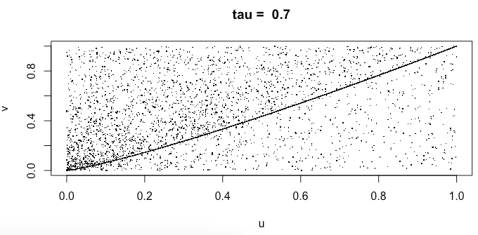
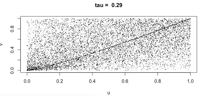
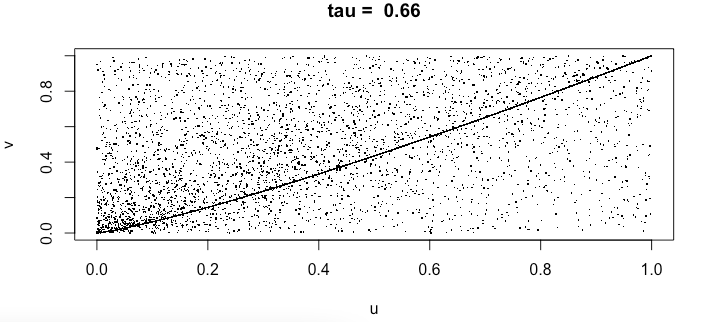
Figure 1: Scatterplots from (34). Top Left: $\theta=0.01$. Bottom: $\theta=0.1$. Top Right: $\theta=1$. Above each graph, the empirical Kendall tau calculated from simulated data is given.

4 Properties and Characterizations of Pseudo Weak Case

The following characterization of distributions satisfying standard weak lack-of-memory property is given in section 3 in Ghurye and Marshall (1984).

Theorem 4.1.

The survival distribution $\bar{F}$ of the vector $\bar{X}=(X_{1},X_{2},\dots,X_{n})$ satisfies standard weak lack-of-memory property if and only if there exists random variables $U$ and $\bar{W}=(W_{1},W_{2},\dots,W_{n})$ such that

1. $\bar{X}=U\bar{e}+\bar{W}$, where $\bar{e}=(1,1,\dots,1)$ is the n-th dimensional unit vector;

2. $U$ and $\bar{W}$ are independent;

3. $P(\min(W_{1},\dots,W_{n})=0)=1$;

4. $U$ has an exponential distribution.

The authors actually show that $U=\min(X_{1},\dots,X_{n})$; moreover, in the bivariate case, they show that the random variables $U=\min(X,Y)$ and $N=\mathbf{1}_{\{X>Y\}}-\mathbf{1}_{\{X<Y\}}$ are independent.
In the same spirit, as for the case of pseudo lack-of-memory property, we get the following result.

Proposition 4.

Let $\bar{F}_{X,Y}$ be a bivariate survival function satisfying pseudo weak lack-of-memory property; moreover, let $\bar{W}=(W_{1},W_{2})=(X-U,Y-U)$ Then:

1. $P(\min(W_{1},W_{2})=0)=1$;

2. $U$ has a pseudo exponential distribution with parameter $\lambda$;

3. $N$ and $U$ are independent;

4. The joint distribution of $U$ and the vector $\bar{W}$ is given by

   $$\begin{split}&P(U\geq u,\bar{W}\geq\bar{w})=\\ &=\begin{cases}\exp_{h}(\lambda u),\ w_{1}\leq 0,w_{2}\leq 0\\ \exp_{h}(\lambda u)\otimes\bar{F}_{1}(w_{1})\left(1-\frac{r_{1}(w_{1})}{\lambda}\right),\ w_{1}>0,w_{2}\leq 0\\ \exp_{h}(\lambda u)\otimes\bar{F}_{2}(w_{2})\left(1-\frac{r_{2}(w_{2})}{\lambda}\right),\ w_{1}\leq 0,w_{2}>0\\ 0,\ w_{1}>0,w_{2}>0\end{cases},\end{split}$$

   where $\bar{F}_{i}(x)=h(\bar{G}_{i}(x)),i=1,2$ and $r_{i}$ is the hazard rate of the survival distribution $\bar{G}_{i},i=1,2$.

Proof.

1. holds true for the same reasons given in Ghurye and Marshall (1984).
For 2., since $\bar{F}_{X,Y}$ satisfies pseudo weak lack-of-memory property,

$$\bar{F}_{U}(u)=P(X\geq u,Y\geq u)=\bar{F}_{X,Y}(u,u)=h(e^{-\lambda u}),u\geq 0.$$

Regarding 3., let us start with the case in which $N=1$: then, by (22),

$$\begin{split}&P(N=1,U\geq u)=P(X>Y\geq u)=\int_{u}^{\infty}\int_{u}^{x}\frac{\partial^{2}\bar{F}}{\partial x\partial y}\ dy\ dx=\\ &=\int_{u}^{\infty}-h^{{}^{\prime}}(e^{-\lambda y}\bar{G}_{1}(x-y))e^{-\lambda y}g_{1}(x-y)\big{|}_{y=u}^{x}\ dx=\\ &=h(e^{-\lambda u})\left(1-\frac{g_{1}(0)}{\lambda}\right).\end{split}$$ (35)

Using equation (26), $P(N=1)=\left(1-\frac{g_{1}(0)}{\lambda}\right),$ so (35) rewrites

$$P(N=1,U\geq u)=P(U\geq u)\ P(N=1).$$

Similar results hold for $N=-1$. In the case in which $N=0$,

$$P(U\geq u,N=0)=P(X=Y\geq u)=h(e^{-\lambda u})\left(\frac{g_{1}(0)+g_{2}(0)}{\lambda}-1\right),$$

thanks to (29); the conclusion follows taking into account that $P(N=0)=\left(\frac{g_{1}(0)+g_{2}(0)}{\lambda}-1\right)$ by (28).
For part 4., it is trivial to show that, if $\bar{w}=(w_{1},w_{2})$, $\bar{F}_{(U,\bar{W})}(u,\bar{w})=h(e^{-\lambda u})$ if $w_{1},w_{2}\leq 0$ and that $\bar{F}_{(U,\bar{W})}(u,\bar{w})=0$ if $w_{1},w_{2}>0$: for this reason, we focus on the cases in which $w_{1}>0$ and $w_{2}\leq 0$ and $w_{1}\leq 0$ and $w_{2}>0$.
For $w_{1}>0$ and $w_{2}\leq 0$, we have that:

$$\begin{split}&P(U\geq u,\bar{W}\geq\bar{w})=P(X\geq u,Y\geq u,X-Y\geq w_{1})=\\ &=P(X\geq w_{1}+u,u\leq Y\leq X-w_{1})=\\ &=\int_{u+w_{1}}^{\infty}\int_{u}^{x-w_{1}}\frac{\partial^{2}\bar{F}}{\partial x\partial y}dy\ dx=\\ &=\int_{u+w_{1}}^{\infty}\left(-h^{{}^{\prime}}(e^{-\lambda y}\bar{G}_{1}(x-y))g_{1}(x-y)e^{-\lambda y}\big{|}_{y=u}^{x-w_{1}}\right)dx=\\ &=h(e^{-\lambda u}\bar{G}_{1}(w_{1}))\left(1-\frac{g_{1}(w_{1})}{\lambda\bar{G}_{1}(w_{1})}\right)=\\ &=\exp_{h}(\lambda u)\otimes\bar{F}_{1}(w_{1})\left(1-\frac{r_{1}(w_{1})}{\lambda}\right).\end{split}$$ (36)

Similarly, if $w_{2}>0$ and $w_{1}\leq 0$, we have

$$P(U\geq u,\bar{W}\geq\bar{w})=\exp_{h}(\lambda u)\otimes\bar{F}_{2}(w_{2})\left(1-\frac{r_{2}(w_{2})}{\lambda}\right).$$ (37)

∎

In theorem 8.1 in Block and Basu (1974), an alternative characterization of the vector $(X,Y)$ possessing standard weak lack-of-memory property is given in terms of the random variables $U$ and $V=X-Y$; in the next Proposition, we extend their characterization to bivariate survival distributions satisfying the pseudo weak lack-of-memory property.

Proposition 5.

Let $F_{X,Y}$ be the bivariate survival function of the vector $(X,Y)$. Then $\bar{F}_{X,Y}$ satisfies pseudo weak lack-of-memory property if and only if

$$\begin{split}&P(U\geq u,V\geq v)=\\ &=\begin{cases}\exp_{h}(\lambda u)+h(e^{-\lambda u}\bar{G}_{2}(-v))\left(\frac{g_{2}(-v)}{\lambda\bar{G}_{2}(-v)}-1\right),u\geq 0,v\leq 0\\ h(e^{-\lambda u}\bar{G}_{1}(v))\left(1-\frac{g_{1}(v)}{\lambda\bar{G}_{1}(v)}\right),u\geq 0,v>0\end{cases}.\end{split}$$ (38)

Proof.

Let us start with the case $v<0$. We have:

$$\begin{split}P(U\geq u,V\geq v)&=\\ &=P(u\leq Y<X)+P(X=Y\geq u)+\\ &+P(X\geq u,X<Y\leq X-v).\end{split}$$

The first probability is already known from equation (35), while the second one is given by (29), so we need to compute only the last one. We get

$$\begin{split}&P(X\geq u,X<Y\leq X-v)=\\ &=\int_{u}^{\infty}\int_{x}^{x-v}\frac{\partial^{2}\bar{F}_{X,Y}(x,y)}{\partial x\partial y}\ dy\ dx=\\ &=\int_{u}^{\infty}h^{{}^{\prime}}(e^{-\lambda x}\bar{G}_{2}(y-x))(-\lambda e^{-\lambda x}\bar{G}_{2}(y-x)+\\ &+e^{-\lambda x}g_{2}(y-x))\big{|}_{y=x}^{x-v}\ dx=\\ &=h(e^{-\lambda u}\bar{G}_{2}(-v))\left(\frac{g_{2}(-v)}{\lambda\bar{G}_{2}(-v)}-1\right)+h(e^{-\lambda u})\left(1-\frac{g_{2}(0)}{\lambda}\right)\end{split}$$

Overall,

$$\begin{split}&P(U\geq u,V\geq v)=h(e^{-\lambda u})+h(e^{-\lambda u}\bar{G}_{2}(-v))\left(\frac{g_{2}(-v)}{\lambda\bar{G}_{2}(-v)}-1\right)\end{split}$$

If $v>0$, by equation (36),

$$P(U\geq u,V\geq v)=h(e^{-\lambda u}\bar{G}_{1}(v))\left(1-\frac{g_{1}(v)}{\lambda\bar{G}_{1}(v)}\right).$$

Conversely, let us suppose that (38) holds true. If $0<x\leq y$, we have that

$$\begin{split}\bar{F}_{X,Y}(x,y)&=\\ &=P(X>x,Y>y,X\geq Y)+P(X>x,Y>y,X<Y)=\\ &=P(U+V>x,U>y,V\geq 0)+\\ &+P(U>x,U-V>y,V<0)=\\ &=P(U>y,V\geq 0)+P(U>x,U-V>y,V<0)=\\ &=P(U>y,V\geq 0)+P(x<U<y,\ x-y<V<U-y)+\\ &+P(U>y,x-y<V<0)+P(U>x,V\leq x-y).\end{split}$$

From (38), $P(U\geq y,V\geq 0)=h(e^{-\lambda u})\frac{g_{2}(0)}{\lambda}$. Moreover,

$$\begin{split}&P(U>y,x-y<V<0)=\\ &=\int_{y}^{\infty}-\lambda e^{-\lambda u}h^{{}^{\prime}}(e^{-\lambda u}\bar{G}_{2}(-v))\ \bar{G}_{2}(-v)\left(\frac{g_{2}(-v)}{\lambda\bar{G}_{2}(-v)}-1\right)\big{|}_{x-y}^{0}\ du=\\ &=h(e^{-\lambda y}\bar{G}_{2}(y-x))\left(\frac{g_{2}(y-x)}{\lambda\bar{G}_{2}(y-x)}-1\right)-h(e^{-\lambda y})\left(\frac{g_{2}(0)}{\lambda}-1\right);\end{split}$$

similarly,

$$\begin{split}&P(x<U<y,\ x-y<V<U-y)=\\ &=h(e^{-\lambda x}\bar{G}_{2}(y-x))\frac{g_{2}(y-x)}{\lambda\bar{G}_{2}(y-x)}-h(e^{-\lambda y})+\\ &-h(e^{-\lambda y}\bar{G}_{2}(y-x))\left(\frac{g_{2}(y-x)}{\lambda\bar{G}_{2}(y-x)}-1\right).\end{split}$$

Finally,

$$\begin{split}&P(U>x,V\leq x-y)=h(e^{-\lambda x}\bar{G}_{2}(y-x))\left(1-\frac{g_{2}(y-x)}{\lambda\bar{G}_{2}(y-x)}\right)\end{split}$$

Summing up all the probabilities above, we get that

$$\bar{F}_{X,Y}(x,y)=h(e^{-\lambda x}\bar{G}_{2}(y-x)),\ 0<x\leq y;$$

similar results hold for $x>y$. ∎

5 Upper and Lower Tail Dependence Coefficients in the Pseudo Weak Case

Given a random vector $(X,Y)$ with copula $C$ and marginal cumulative distribution functions $F_{X}$ and $F_{Y}$, we recall that the upper tail dependence coefficient $\lambda_{U}$ can be written as

$$\lambda_{U}=\lim_{u\rightarrow 1^{-}}P[F_{X}(X)>u|\ F_{Y}(Y)>u]=\lim_{u\rightarrow 1^{-}}\frac{1-2u+C(u,u)}{1-u};$$

analogously, the lower tail dependence coefficient $\lambda_{L}$ is given by

$$\lambda_{L}=\lim_{u\rightarrow 0^{+}}P[F_{X}(X)<u|\ F_{Y}(Y)<u]=\lim_{u\rightarrow 0^{+}}\frac{C(u,u)}{u}.$$

Thanks to (23), the survival copula associated to the survival distribution satisfying pseudo weak lack-of-memory property is $C^{F}(u,v)=h(C^{G}(h^{-1}(u),h^{-1}(v))$. The following Propositions in Durante et al. (2010) applies to this case.

Proposition 6.

Let $C$ be a copula with finite lower tail dependence coefficient $\lambda_{L}(C)$. Moreover, let $\psi$ be an isomorphism of $[0,1]$ such that $C_{\psi}(u,v)=\psi\{C[\psi^{-1}(u),\psi^{-1}(v)]\}$ is again a copula. Then, if

$$\lim_{t\rightarrow 0^{+}}\frac{\psi(t)}{t^{\alpha}}=b\in(0,+\infty)$$

for some $\alpha>0$, then $\lambda_{L}(C_{\psi})=(\lambda_{L}(C))^{\alpha}$.

Proposition 7.

Let $C$ be a copula with finite upper tail dependence coefficient $\lambda_{U}(C)$. Moreover, let $\psi$ be an isomorphism of $[0,1]$ such that $C_{\psi}(u,v)=\psi\{C[\psi^{-1}(u),\psi^{-1}(v)]\}$ is again a copula. Then, if

$$\lim_{t\rightarrow 1^{-}}\frac{1-\psi(t)}{(1-t)^{\alpha}}=b\in(0,+\infty)$$

for some $\alpha>0$, then $\lambda_{U}(C_{\psi})=2-(2-\lambda_{U}(C))^{\alpha}$.

So, in order to apply these results, we determine lower and upper tail dependence coefficients in the standard weak case, assuming that the marginal survival functions of the distribution are identical. If $\bar{G}_{1}=\bar{G}_{2}=\bar{G}$, from (24), we have

$$\begin{split}\bar{C^{G}}(u,v)&=\\ &=e^{-\lambda\bar{G}^{-1}(v)}\bar{G}(\bar{G}^{-1}(u)-\bar{G}^{-1}(v))1_{u<v}+\\ &+e^{-\lambda\bar{G}^{-1}(u)}\bar{G}(\bar{G}^{-1}(v)-\bar{G}^{-1}(u))1_{u\geq v}.\end{split}$$ (39)

By the system of inequalities (14), we know that this is a survival copula if and only if $\lambda\leq 2g(0)$ and $\frac{\partial\log(g(z))}{\partial z}\geq-\lambda,\ \forall z\geq 0$.

Proposition 8.

Let $(X,Y)$ be a random vector with survival copula $\bar{C^{G}}$ of type (39) and let $g(x)=-\bar{G}^{{}^{\prime}}(x),\ x\geq 0$ such that $\lambda\leq 2g(0)$ and $\frac{\partial\log(g(z))}{\partial z}\geq-\lambda,\ \forall z\geq 0$. Then:

1. $\lambda_{L}=0$, if $\bar{G}$ is heavy tailed, id est $\lim_{x\to\infty}\frac{\bar{G}(x)}{e^{-\lambda x}}=+\infty,\ \forall\lambda>0$.

2. $\lambda_{U}=2-\frac{\lambda}{g(0)}.$

Proof.

For 1., we have

$$\lambda_{L}=\lim_{u\rightarrow 0^{+}}\frac{\bar{C^{G}}(u,u)}{u}=\lim_{u\rightarrow 0^{+}}\frac{e^{-\lambda\bar{G}^{-1}(u)}}{u}.$$

Setting $x=\bar{G}^{-1}(u)$, we have

$$\lambda_{L}=\lim_{x\rightarrow\infty}\frac{e^{-\lambda x}}{\bar{G}(x)}=0.$$

Regarding 2., we can write

$$\begin{split}\lambda_{U}&=\lim_{u\rightarrow 1^{-}}\frac{1-2u+\bar{C^{G}}(u,u)}{1-u}=2+\lim_{u\rightarrow 1^{-}}\frac{e^{-\lambda\bar{G}^{-1}(u)}-1}{1-u}=\\ &=2+\lim_{x\rightarrow 0^{+}}\frac{e^{-\lambda x}-1}{1-\bar{G}(x)}=2-\lambda\lim_{x\rightarrow 0^{+}}\frac{x}{G(x)},\end{split}$$

from which the conclusion follows. ∎

In the case in which the marginal distribution is light-tailed, the value of the lower tail dependence coefficient depends on the functional form of the distribution.

Using Propositions 6 and 7, we are able to find the lower and the upper tail dependence coefficients for different choices of the common marginal survival functions and of the generator $h$, as shown in the following Examples.

Example 3.

Let $(X,Y)$ be a random vector satisfying bivariate pseudo-weak lack-of-memory property with marginal survival functions $\bar{F}_{i}(x)=\exp_{h}(\mu x)$, $i=1,2$, $\mu\leq\lambda\leq 2\mu$.
If $h=id$, we get the standard Marshall Olkin distribution: since $\bar{G}_{i}(x)=e^{-\mu_{i}x}$, we can show that $\lambda_{L}(\bar{C}^{G})=0$ if $\mu<\lambda\leq 2\lambda$ and that $\lambda_{L}(\bar{C}^{G})=1$ if $\lambda=\mu$.
Moreover, using Proposition 8, we can easily prove that $\lambda_{U}(\bar{C}^{G})=2-\frac{\lambda}{\mu}\in[0,1]$.
If $h(x)=1-\left(\frac{\tan(\theta(1-x))}{\tan(\theta)}\right)^{\beta},-\frac{\pi}{2}<\theta<0,\ 0<\beta<1$, then $h$ is a convex bjection of the unit interval and condition given in Proposition (6) is satisfied with $\alpha=1$ and with $b=\frac{2\theta\beta}{\sin(2\theta)}$, implying that $\lambda_{L}(\bar{C}_{h})=\lambda_{L}(\bar{C}^{G})$.
Moreover, it satisfies also Proposition (7) with parameters $\alpha=\beta$ and $b=\left(\frac{\theta}{\tan(\theta)}\right)^{\beta}$: so $\lambda_{U}(\bar{C}_{h})=2-\left(\frac{\lambda}{\mu}\right)^{\beta}\in[0,1]$.

Example 4.

Let $(X,Y)$ be a random vector satisfying bivariate pseudo-weak lack-of-memory property with marginal survival functions $\bar{F}_{i}(x)=h((1+x)^{-\gamma})$, $i=1,2$, $\gamma\geq 1$, $\gamma+1\leq\lambda\leq 2\gamma$.
If $h=id$, by Proposition 8, it follows that $\lambda_{L}(\bar{C}^{G})=0$.
Moreover, using Proposition 8, we can easily prove that $\lambda_{U}(\bar{C}^{G})=2-\frac{\lambda}{\gamma}\in[0,1]$. If $h(x)=1-\left(\frac{e^{\theta(1-x)}-1}{e^{\theta}-1}\right)^{\beta},\ \theta<0,\ 0<\beta<1$, then $h$ is a convex bjection of the unit interval $[0,1]$ and condition given in Proposition (6) is satisfied with $\alpha=1$ and with $b=\frac{\theta\beta e^{\theta}}{e^{\theta}-1}$, implying that $\lambda_{L}(\bar{C}_{h})=\lambda_{L}(\bar{C}^{G})=0$.
Moreover, it satisfies also Proposition (7) with parameters $\alpha=\beta$ and $b=\frac{\theta}{(e^{\theta}-1)^{\beta}}:$ so $\lambda_{U}(\bar{C}_{h})=2-\left(\frac{\lambda}{\gamma}\right)^{\beta}\in[0,1]$.
Using conditional distribution method, we simulate data with parameters $\gamma=1.5$, $\lambda=2.6$ and $\theta=-1$ from the survival distribution function

$$\begin{split}\bar{F}_{X,Y}(x,y)&=\\ &=1-\left(\frac{e^{\theta(1-(1+x-y)^{-\gamma})}-1}{e^{\theta}-1}\right)^{\beta}1_{x\geq y}+\\ &+1-\left(\frac{e^{\theta(1-(1+y-x)^{-\gamma})}-1}{e^{\theta}-1}\right)^{\beta}1_{x<y}:\end{split}$$ (40)

the scatterplots are given below for three different values of $\beta$.

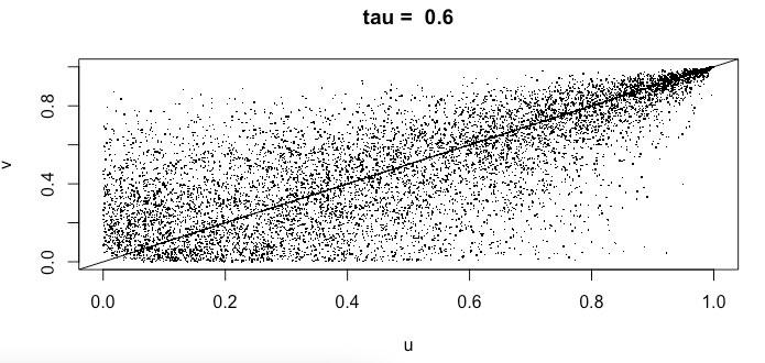
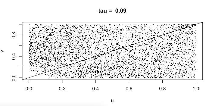
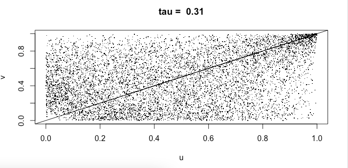
Figure 2: Scatterplots from (40). Top Left: $\beta=0.3$. Bottom: $\beta=0.6$. Top Right: $\beta=0.9$. Above each graph, the empirical Kendall tau calculated from simulated data is given.

6 Conclusions

In this paper, we have generalized standard lack-of-memory properties by substituting into (6) and (5) the standard product by the pseudo product $\otimes$: we have discussed the conditions under which the solutions of the obtained functional equations (9) and (8) are bivariate survival functions. Then our attention focused on the solution of (8): we have proved that it has a singularity along the line $x=y$ and we have analysed how the probability mass is distributed along that line. Moreover, we have characterized this distribution in terms of the random variables $U=\min(X,Y)$ and $V=X-Y$; we have also found the joint distribution of the vector $(N,U,\bar{W})$, where $N=\mathbf{1}_{\{X>Y\}}-\mathbf{1}_{\{X<Y\}}$ and $\bar{W}=(X-U,Y-U).$ Finally, we have analysed the dependence structure of the distribution satisfying (8) showing that its associated survival copula can be written in terms of the survival copula of the distribution which satisfies the standard weak lack-of-memory property: in particular, we have determined analytically the lower and the upper tail dependence coefficients and we have computed the empirical Kendall tau from data generated from these distributions using conditional distribution method.
The analysis of applications to reliability and insurance modelling is part of the research on this topic and of the next future work.

References

- [1] J.Aczel. ”Lectures on functional equations and their applications”. Academic Press (1966), New York.
- [2] A.V. Asimit, E. Furman, R. Vernic. ”On a multivariate Pareto distribution”. In: Insurance: Mathematics and Economics (2010), Volume 46, pp. 308–316.
- [3] H.W. Block, A.P. Basu. ”A continuous bivariate exponential extension”. In: Journal of the American Statistical Association (1974), Volume 69, pp. 1031-1037.
- [4] Fabrizio Durante, Rachele Foschi, Peter Sarkoci. ”Distorted Copulas: Constructions and Tail Dependence”. In: Communications in Statistics - Theory and Methods (2010), Volume 39, Issue 12, pp. 2288-2301
- [5] C.Genest,N.Kolev. ” A law of uniform seniority for dependent lives”. In: Scandinavian Actuarial Journal (2021), Volume 2021, pp. 726-743
- [6] S.G. Ghurye, A.W. Marshall. ”Shock Processes with Aftereffects and Multivariate Lack-of-Memory Property”. In: Journal of Applied Probability (1984), Volume 21, pp. 786-801.
- [7] E.P. Klement R. Mesiar E. Pap. ”Triangular norms. Position paper III: continuous t-norms”. In: Fuzzy Sets and System (2004), Volume 145, pp. 439–454.
- [8] E.P. Klement R. Mesiar E. Pap. ”Transformations of copulas”. In: Kybernetika (2005), Volume 41, pp. 425–434.
- [9] X.Li, F.Pellerey. ”Generalized Marshall-Olkin distributions and related bivariate aging properties”. In: Journal of Multivariate Analysis (2011), Volume 102, pp. 1399-1409.
- [10] C.H. Ling. ”Representation of associative functions”. In: Publicationes Mathematicae Debrecen (1965), Volume 12, pp. 189-212.
- [11] J.C. Lu. ”Weibull extension of the Freund and Marshall–Olkin bivariate exponential model”. In: IEEE Transactions on Reliability (1989), Volume 38, pp. 615–619.
- [12] A.Marshall I.Olkin. ”A multivariate exponential distribution”. In: Journal of the American Statistical Association (1967), Volume 62, pp. 30–44.
- [13] T.Mikosch. ”Non-Life Insurance Mathematics: an Introduction with the Poisson Process”. In: Springer (2009), Second Edition.
- [14] P.Muliere, M.Scarsini. ”Characterization of a Marshall-Olkin Type Class of Distributions”. In:Annals of the Institute of Statistical Mathematics (1987), Volume 39, pp. 429-441.
- [15] S.Mulinacci. “Archimedean-based Marshall-Olkin Distributions and Re- lated Dependence Structures”. In: Methodology and Computing in Applied Probability (2018), Volume 20, pp. 205–236.
- [16] R.B. Nelsen. ”Dependence modeling with Archimedean copulas” In: Proceedings of the Second Brazilian Conference on Statistical Modelling in Insurance and Finance, Institute of Mathematics and Statistics, University of São Paulo (2005), pp. 45-54
- [17] R.B.Nelsen. ”An introduction to copulas”. In: Springer Series in Statistics (2006), Second Edition.
- [18] B. Schweizer and A. Sklar. ”Associative functions and statistical triangle inequalities”. In: Publicationes Mathematicae Debrecen (1961), Volume 8, pp.169-186.