Nonlocal Andreev transport through a quantum dot in a magnetic field:
Interplay between Kondo, Zeeman, and Cooper-pair correlations

Abstract

We study the nonlocal magnetotransport through a strongly correlated quantum dot, connected to multiple terminals consisting of two normal and one superconducting (SC) leads. Specifically, we present a comprehensive view on the interplay between the crossed Andreev reflection (CAR), the Kondo effect, and the Zeeman splitting at zero temperature in the large SC gap limit. The ground state of this network shows an interesting variety, which varies continuously with the system parameters, such as the coupling strength $\Gamma_{S}$ between the SC lead and the quantum dot, the Coulomb repulsion $U$, the impurity level $\varepsilon_{d}$, and the magnetic field $b$. We show, using the many-body optical theorem which is derived from the Fermi-liquid theory, that the nonlocal conductance is determined by the transmission rate of the Cooper pairs $\mathcal{T}_{\mathrm{CP}}=\frac{1}{4}\sin^{2}\Theta\,\sin^{2}\bigl{(}\delta_{\uparrow}+\delta_{\downarrow})$ and that of the Bogoliubov particles $\mathcal{T}_{\mathrm{BG}}=\frac{1}{2}\sum_{\sigma}\sin^{2}\delta_{\sigma}$. Here, $\delta_{\sigma}$ is the phase shift of the renormalized Bogoliubov particles, and $\Theta\equiv\cot^{-1}(\xi_{d}/\Gamma_{S})$ is the Bogoliubov-rotation angle in the Nambu pseudo spin space, with $\xi_{d}=\varepsilon_{d}+U/2$. It is also demonstrated, using Wilson’s numerical renormalization group approach, that the CAR is enhanced in the crossover region between the Kondo regime and the SC-proximity-dominated regime at zero magnetic field. The magnetic fields induce another crossover between the Zeeman-dominated regime and the SC-dominated regime, which occurs when the renormalized Andreev resonance level of majority spin crosses the Fermi level. We find that the CAR is enhanced and becomes less sensitive to magnetic fields in the SC-dominated regime close to the crossover region spreading over the angular range of $\pi/4\lesssim\Theta\lesssim 3\pi/4$. At the level crossing point, a spin-polarized current flows between the two normal leads, and it is significantly enhanced in the directions of $\Theta\simeq 0$ and $\Theta\simeq\pi$ where the SC proximity effect is suppressed.

I Introduction

Quantum dots (QD) connected to multi terminal networks consisting of normal and superconducting (SC) leads is one of the active fields of current research. In such networks, the quantum coherence and entanglements can be probed through the Andreev reflection Hofstetter et al. (2009); Schindele et al. (2012); Das et al. (2012); Schindele et al. (2014); Fülöp et al. (2014); Tan et al. (2015); Borzenets et al. (2016); Tan et al. (2021); Golubev and Zaikin (2007); Eldridge et al. (2010); Sánchez et al. (2018); Wrześniewski and Weymann (2017); Rech et al. (2012); Walldorf et al. (2018); Hussein et al. (2019); Wójcik and Weymann (2019); Walldorf et al. (2020); Lee et al. (2014); Bordoloi et al. (2022) and Josephson effect. Choi et al. (2000); Wang and Hu (2011); Deacon et al. (2015); Padurariu et al. (2017); Yokoyama and Nazarov (2015); Ueda et al. (2019)

In particular, the crossed Andreev reflection (CAR) is one of the most interesting processes caused by a Cooper-pair tunneling in which an incident electron entering from a normal lead forms a Cooper pair with another electron from the other normal leads to tunnel into the SC leads, leaving a hole in the normal lead where the second electron came from. The time-reversal process of the CAR corresponds to a splitting of a Cooper pair that is emitted from the SC lead into two entangled electrons penetrating the different normal leads. The CAR and the Cooper-pair splitting have also been studied in the multi-terminal systems without quantum dots. Cadden-Zimansky and Chandrasekhar (2006); Lesovik, G. B. et al. (2001); Russo et al. (2005); Yeyati et al. (2007); Cadden-Zimansky et al. (2009); Wei and Chandrasekhar (2010); Golubev and Zaikin (2019); Kirsanov et al. (2019); Ranni et al. (2021)

Quantum dots give a variety to the transport properties of multi-terminal systems, through the tunable parameters such as electron correlations, resonant-level positions, and local magnetic fields which can polarize the spins of electrons. The strong electron correlations induce an interesting crossover between the Kondo singlet and the Cooper-pair singlet. Yoshioka and Ohashi (2000); Tanaka et al. (2007a); Buizert et al. (2007); Deacon et al. (2010a, b); Yamada et al. (2011); Governale et al. (2008); Oguri et al. (2013); Koga (2013); Domański et al. (2017); Vecino et al. (2003); Oguri et al. (2004); Tanaka et al. (2007b); Lee et al. (2022); Pillet et al. (2013); Kadlecová et al. (2017); Pokorný and Žonda (2023) Furthermore, the magnetic field induces a crossover occurring between the Kondo singlet state and the spin-polarized state due to the Zeeman splitting of discrete energy levels of quantum dots, which has recently been revisited to find that the three-body Fermi-liquid corrections play an essential role in the crossover region. Filippone et al. (2018); Oguri and Hewson (2018)

The CAR contributions can be probed through the nonlocal conductance for the current flowing from the QD towards one of the normal drain electrode when the bias voltage is applied to the source electrode. Hofstetter et al. (2009); Schindele et al. (2014); Fülöp et al. (2014); Tan et al. (2015) However, the nonlocal current also includes the contributions of the single-electron-tunneling process, in which an incident electron from the source electrode transmits directly towards the drain electrode through the QD. In order to observe the CAR contributions, it is important to find some sweet spots in the parameter space, at which the superconducting proximity effect dominates the nonlocal current and enhances the Cooper-pair tunneling by reconciling it with the other effects from electron correlations and magnetic fields.

The CAR in a single correlated quantum dot has theoretically been studied over a decade, particularly for a three-terminal QD connected to two normal and one superconducting leads. In the early stage, Futterer et al.Futterer et al. (2009) and Michałek et al.Michałek et al. (2013, 2015) demonstrated some behaviors of the nonlocal transport conductance typical to this three-terminal configuration,Michałek et al. (2015) taking also into account the Coulomb interaction with a generalized master equationFutterer et al. (2009) or the equation-of-motion method.Michałek et al. (2013) It has been extended to the configuration in which the normal leads are replaced by ferromagnetic metals and has been investigated intensively, using also the methods such as the real-time diagrammatic method and the numerical renormalization group (NRG). Futterer et al. (2009); Trocha and Wrześniewski (2018); Weymann and Trocha (2014); Wójcik and Weymann (2014); Weymann and Wójcik (2015)

Effects of the Zeeman splitting induced by the external magnetic field applied to quantum dots have also been theoretically investigated, mainly for two-terminal systems in which a quantum dot is connected to a single paramagnetic normal and a SC lead so far.Zhao and Wang (2001); Górski et al. (2020); Yamada et al. (2007); Domański et al. (2008, 2016); Žitko et al. (2015) Specifically, these theories addressed such subjects as the field dependence of the Andreev transport,Zhao and Wang (2001); Górski et al. (2020) the role of the Coulomb interaction in this configuration, Yamada et al. (2007); Domański et al. (2008, 2016) and the quantum phase transition between the spin-singlet and -doublet ground states.Žitko et al. (2015) However, it is still not fully clarified how the CAR contributions evolve at low energies in a wide parameter space of the multi-terminal networks, with and without magnetic fields.

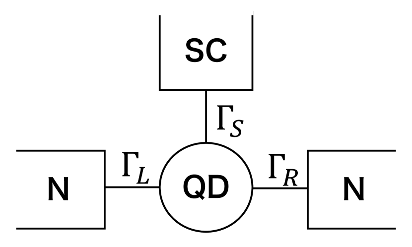
Figure 1: Single quantum dot (QD) connected to two normal leads (N) and one superconductor lead (SC). $\Gamma_{L}$, $\Gamma_{R}$, and $\Gamma_{S}$ represent the coupling strengths of the QD with the left ($L$), the right ($R$), and the SC leads, respectively. The contributions of the normal tunnelings are given by $\Gamma_{N}=\Gamma_{L}+\Gamma_{R}$.

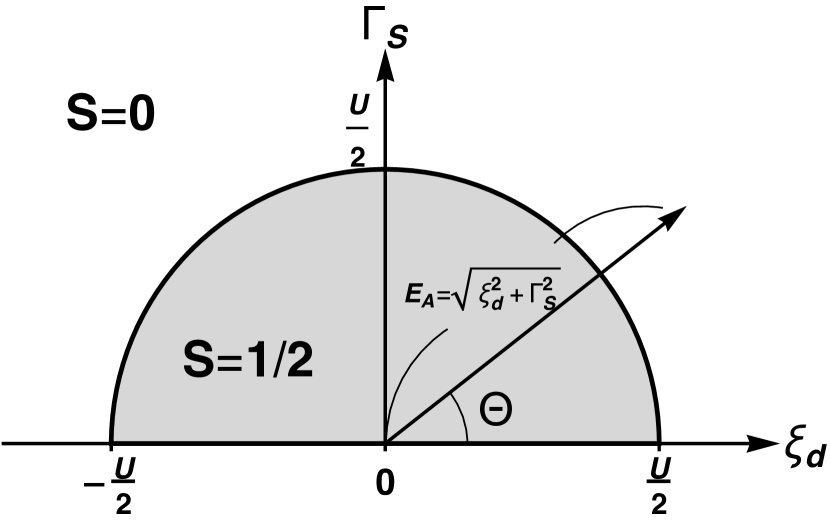
Figure 2: Parameter space of $H_{\mathrm{eff}}$ at zero magnetic field $b=0$, defined in Eqs. (50) and (8). The semicircle represents the line along which the energy of the Andreev level $E_{A}\equiv\sqrt{\xi_{d}^{2}+\Gamma_{S}^{2}}$ coincides with one-half of the Coulomb interaction $U/2$, where $\xi_{d}\equiv\varepsilon_{d}+U/2$. In the atomic limit $\Gamma_{N}=0$, the ground state is a magnetic spin doublet inside the semicircle, which eventually is screened by conduction electrons to form the Kondo singlet when the tunnel coupling $\Gamma_{N}$ is switched on, whereas the ground state is a spin singlet due to the Cooper paring outside the circle. $\Theta$ is the Bogoliubov-rotation angle, which parametrizes the contributions of the Andreev scattering on the transport coefficients.

The purpose of this paper is to provide a comprehensive view of the Andreev transport through a strongly-correlated quantum state, the characteristics of which vary due to the interplay between the Kondo, Zeeman, and Cooper-pair correlations. To this end, we calculate the transport coefficients, using the Fermi-liquid theory Nozières (1974); Yamada (1975a, b); Shiba (1975); Yoshimori (1976) in conjunction with Wilson’s numerical renormalization group (NRG). Specifically, we consider a three-terminal quantum dot connected to two normal and one superconducting leads, as illustrated in Fig. 1, in the large SC gap limit.Tanaka et al. (2007a) We first of all derive the optical theorem for the CAR at zero temperature, using the Fermi-liquid theory that describes the interacting Bogoliubov particles moving throughout the entire system. It elucidates the fact that the nonlocal conductance is determined by the transmission rate of Cooper pairs $\mathcal{T}_{\mathrm{CP}}=\frac{1}{4}\sin^{2}\Theta\,\sin^{2}\bigl{(}\delta_{\uparrow}+\delta_{\downarrow})$ and that of the Bogoliubov particles $\mathcal{T}_{\mathrm{BG}}=\frac{1}{2}\sum_{\sigma}\sin^{2}\delta_{\sigma}$. Here, $\Theta\equiv\cot^{-1}(\xi_{d}/\Gamma_{S})$ is the angular coordinate in the $\xi_{d}\equiv\varepsilon_{d}+U/2$ vs $\Gamma_{S}$ plane shown in Fig. 2, and $\varepsilon_{d}$ and $U$ are the discrete level and the Coulomb interaction of electrons in the QD, respectively, and $\Gamma_{S}$ is the coupling strength between the QD and SC lead. In this case, the phase shift $\delta_{\sigma}$ of the interacting Bogoliubov particles does not depend on the angle $\Theta$ but varies along the radial coordinate $E_{A}=\sqrt{\xi_{d}^{2}+\Gamma_{S}^{2}}$.

We also calculate the transmission rate $\mathcal{T}_{\mathrm{CP}}$ and $\mathcal{T}_{\mathrm{BG}}$ with the NRG in a wide range of the parameter space. It is demonstrated that, at zero magnetic field, the CAR contributions are significantly enhanced near the crossover region between the Kondo regime and the SC-proximity-dominated regime. Specifically, it takes place in a crescent-shaped region spreading over the range of $U/2\lesssim E_{A}\lesssim U/2+\Gamma_{N}$ in the radial direction and $\pi/4\lesssim\Theta\lesssim 3\pi/4$ in the angular direction: $\Gamma_{N}$ is the resonance width due to the tunneling between the QD and normal leads. When a magnetic field is applied, another crossover occurs between the Zeeman-dominated regime and the SC-proximity-dominated regime when the spin-polarized Andreev level crosses the Fermi level. We find that the CAR-dominated transport taking place in the crescent region is less sensitive to magnetic fields, and it emerges as a flat valley structure in the magnetic-field dependence of the nonlocal conductance. This parameter region provides an optimal condition for observing the Cooper-pair tunneling, i.e., a sweet spot, especially in the direction of $\Theta\simeq\pi/2$ where the Cooper pairs are most entangled and become equal-weight linear combinations of an electron and a hole.

This paper is organized as follows. In Sec. II, we introduce an Anderson impurity model for quantum dots connected to SC and normal leads, and rewrite the Hamiltonian and the Green’s function in terms of interacting Bogoliubov particles. Then, the optical theorem and the formula for the nonlocal conductance are derived at zero temperature using the Fermi-liquid description for the interacting Bogoliubov particles in Sec. III. We investigate the CAR contributions to the nonlocal conductance, using the NRG, at zero and finite magnetic fields in Secs. IV and V, respectively. Summary and discussion are given in Sec. VI.

II Fermi-liquid description for interacting Bogoliubov particles

In this section, we show how the contributions of the CAR to the nonlocal conductance of the multi-terminal network can be described in the context of the Fermi-liquid theory for the interacting Bogoliubov particles at zero temperature.Tanaka et al. (2007a)

II.1 Anderson impurity model for the CAR

We start with an Anderson impurity model for a single quantum dot (QD) connected to two normal (N) and one superconducting (SC) leads, as shown in Fig. 1:

$$H\,= \ \,H_{\mathrm{dot}}\,+\,H_{\text{N}}\,+\,H_{\text{TN}}\,+\,H_{\text{S}}+H_{\text{TS}}\,,$$ (1)

$$H_{\mathrm{dot}}= \ \xi_{d}\bigl{(}n_{d}-1\bigr{)}-b\,\bigl{(}n_{d,\uparrow}-n_{d,\downarrow}\bigr{)}\,+\frac{U}{2}\bigl{(}n_{d}-1\bigr{)}^{2},$$ (2)

$$H_{\text{N}}= \ \sum_{\nu=L,R}\sum_{\sigma}\int_{-D}^{D}\!d\varepsilon\,\varepsilon\,c^{\dagger}_{\varepsilon,\nu,\sigma}c_{\varepsilon,\nu,\sigma},$$ (3)

$$H_{\text{TN}}= \ \sum_{\nu=L,R}v_{\nu}\sum_{\sigma}\int_{-D}^{D}\!d\varepsilon\,\sqrt{\rho_{c}}\,\Bigl{(}c^{\dagger}_{\varepsilon,\nu,\sigma}d_{\sigma}+\mathrm{H.c.}\Bigr{)},$$ (4)

$$H_{\text{S}}= \ \sum_{\sigma}\!\int_{-D_{S}}^{D_{S}}\!\!d\varepsilon\,\varepsilon\,s^{\dagger}_{\varepsilon,\sigma}s_{\varepsilon,\sigma}$$

$$\quad\ +\int_{-D_{S}}^{D_{S}}\!\!d\varepsilon\left(\Delta_{S}\,s^{\dagger}_{\varepsilon,\uparrow}s^{\dagger}_{\varepsilon,\downarrow}+\mathrm{H.c.}\right),$$ (5)

$$H_{\text{TS}}= \ v_{\text{S}}\sum_{\sigma}\!\int_{-D_{S}}^{D_{S}}\!\!d\varepsilon\,\sqrt{\rho_{S}}\,\Bigl{(}s^{\dagger}_{\varepsilon,\sigma}d_{\sigma}+\mathrm{H.c.}\Bigr{)}.$$ (6)

Here, $H_{\mathrm{dot}}$ describes the QD part: $\xi_{d}\equiv\varepsilon_{d}+{U}/{2}$, with $\varepsilon_{d}$ the discrete energy level, $U$ the Coulomb interaction, and $b$ ($\equiv\mu_{B}B)$ the Zeeman energy due to the magnetic field $B$ applied to the QD, with $\mu_{B}$ the Bohr magneton. $d^{\dagger}_{\sigma}$ is the creation operator for an electron with spin $\sigma$, and $n_{d}\equiv n_{d,\uparrow}+n_{d,\downarrow}$ is the number operator with $n_{d,\sigma}\equiv d^{\dagger}_{\sigma}d_{\sigma}$. A constant energy shift, which does not affect the physics, is included in Eq. (2) in order to describe clearly that the system has the electron-hole symmetry at $\xi_{d}=0$.

$H_{\text{N}}$ describes the conduction electrons in the normal leads, the density of states of which is assumed to be flat $\rho_{c}=1/(2D)$, with $D$ the half-width of the bands. $c^{\dagger}_{\varepsilon,\nu,\sigma}$ is the creation operator for conduction electrons with spin $\sigma$ and energy $\varepsilon$. The operators for conduction electrons satisfy the following anti-commutation relation that is normalized by the Dirac delta function: $\{c_{\varepsilon,\nu,\sigma},c^{\dagger}_{\varepsilon^{\prime},\nu^{\prime},\sigma^{\prime}}\}=\delta_{\nu\nu^{\prime}}\,\delta_{\sigma\sigma^{\prime}}\delta(\varepsilon-\varepsilon^{\prime})$. $H_{\text{TN}}$ describes the tunnel couplings between the QD and the normal leads. The level broadening of the discrete energy level in the QD is given by $\Gamma_{N}\equiv\Gamma_{L}+\Gamma_{R}$, with $\Gamma_{\nu}\equiv\pi\rho_{c}v_{\nu}^{2}$ the contributions of the two normal leads on the left $\nu=L$ and right $\nu=R$.

$H_{\text{S}}$ and $H_{\text{TS}}$ describe the contributions of the superconducting lead with an $s$-wave SC gap $\Delta_{S}\equiv\left|\Delta_{S}\right|\,e^{i\phi_{S}}$: $s^{\dagger}_{\varepsilon,\sigma}$ is the creation operator for electrons in the SC lead, with $D_{S}$ the half-band width and $\rho_{S}=1/(2D_{S})$. One of the key parameters for the SC proximity effects is $\Gamma_{S}\equiv\pi\rho_{S}v_{\text{S}}^{2}$, i.e., the coupling strength between the QD and the SC lead.

In this paper, we study the crossed Andreev reflection occurring at low energies, much lower than the SC energy gap. To this end, we consider the large gap limit $\left|\Delta_{S}\right|\to\infty$, which is taken at $\left|\Delta_{S}\right|\ll D_{S}$ keeping $\Gamma_{S}$ constant.Tanaka et al. (2007a) In this case, the superconducting proximity effects can be described by the pair potential penetrating into the QD:

$$\Delta_{d}\equiv\Gamma_{S}\,e^{i\phi_{S}}\,.$$ (7)

The Coulomb interaction $U$ induces the correlation effects for electrons in the QD and the symmetrized linear combination of the conduction bands defined in Eq.  (46), which can be described by an effective Hamiltonian $H_{\mathrm{eff}}$ given in Eq. (50) (see Appendix A). Furthermore, carrying out the Bogoliubov rotation defined in Eq. (53), it can be transformed further into a system of interacting Bogoliubov particles described by a standard Anderson model:

$$H_{\mathrm{eff}}= \ E_{A}\left(\sum_{\sigma}\gamma^{\dagger}_{d,\sigma}\gamma_{d,\sigma}-1\right)-b\,\Bigl{(}\gamma^{\dagger}_{d,\uparrow}\gamma_{d,\uparrow}-\gamma^{\dagger}_{d,\downarrow}\gamma_{d,\downarrow}\Bigr{)}$$

$$+\frac{U}{2}\left(\sum_{\sigma}\gamma^{\dagger}_{d,\sigma}\gamma_{d,\sigma}-1\right)^{2}+\sum_{\sigma}\int_{-D}^{D}\!d\varepsilon\,\varepsilon\ \gamma^{\dagger}_{\varepsilon,\sigma}\gamma_{\varepsilon,\sigma}$$

$$+v_{N}\sum_{\sigma}\int_{-D}^{D}\!d\varepsilon\,\sqrt{\rho_{c}}\,\left(\gamma^{\dagger}_{\varepsilon,\sigma}\gamma_{d,\sigma}+\mathrm{H.c.}\right)\,,$$ (8)

$$N_{\gamma}= \ \sum_{\sigma}\gamma^{\dagger}_{d,\sigma}\gamma_{d,\sigma}+\sum_{\sigma}\int_{-D}^{D}\!d\varepsilon\,\gamma^{\dagger}_{\varepsilon,\sigma}\gamma_{\varepsilon,\sigma}\,.$$ (9)

Here, $E_{A}\equiv\sqrt{\xi_{d}^{2}+\Gamma_{S}^{2}}$ is the effective impurity level, and $v_{N}\equiv\sqrt{v_{L}^{2}+v_{R}^{2}}$. The operators $\gamma_{d,\sigma}$ and $\gamma_{\varepsilon,\sigma}$ describe the Bogoliubov particles in the dot and the symmetrized part of the conduction band, respectively. The effective Hamiltonian conserves the total number of the Bogoliubov particles $N_{\gamma}$, reflecting the $U(1)$ symmetry along the principal axis in the Nambu pseudo-spin space.

Figure 2 illustrates the parameter space of $H_{\mathrm{eff}}$ at zero magnetic field $b=0$. For finite $\Gamma_{N}$, the Kondo screening due to the normal conduction electrons occurs inside the semicircle region, at which the impurity level is occupied by a single Bogoliubov particle: $Q\simeq 1.0$ with

$$Q\, \equiv\,Q_{\uparrow}+Q_{\downarrow},\qquad Q_{\sigma}\,\equiv\,\left\langle\gamma^{\dagger}_{d,\sigma}\gamma_{d,\sigma}\right\rangle.$$ (10)

Bogoliubov particles show also the valence-fluctuation behavior near $E_{A}\simeq U/2$, at which the crossover between the Kondo singlet and the superconducting singlet occurs. The Bogoliubov rotation angle corresponds to $\Theta=\cot^{-1}(\xi_{d}/\Gamma_{S})$ shown in Fig. 2. In particular, the crossed Andreev scattering is enhanced in the angular range of $\pi/4\lesssim\Theta\lesssim 3\pi/4$ outside the semicircle $E_{A}\gtrsim U/2$, as discussed later in Secs. IV and V.

II.2 Renormalized Bogoliubov quasiparticles

In this work, we calculate the nonlocal conductance for the current flowing into the drain electrode, using the retarded Green’s function for electrons in the QD:

$$\!\!\!\bm{G}^{r}_{dd}(\omega)\equiv-i\int_{0}^{\infty}\!dt\,e^{i\left(\omega+i0^{+}\right)t}$$

$$\qquad\qquad\ \ \times\begin{pmatrix}\left\langle\left\{d_{\uparrow}(t),\,d^{\dagger}_{\uparrow}\right\}\right\rangle&\left\langle\left\{d_{\uparrow}(t),\,d_{\downarrow}\right\}\right\rangle\\ \left\langle\left\{d^{\dagger}_{\downarrow}(t),\,d^{\dagger}_{\uparrow}\right\}\right\rangle&\left\langle\left\{d^{\dagger}_{\downarrow}(t),\,d_{\downarrow}\right\}\right\rangle\rule{0.0pt}{17.07182pt}\end{pmatrix}.$$ (11)

Here, $\langle\cdots\rangle$ denotes the thermal average at equilibrium. This matrix Green’s function can be diagonalized with the Bogoliubov transformation:

$$\bm{\mathcal{U}}^{\dagger}\,\bm{G}^{r}_{dd}(\omega)\ \bm{\mathcal{U}}\, =\,\begin{pmatrix}G^{r}_{\gamma,\uparrow}(\omega)&0\\ 0&-G^{a}_{\gamma,\downarrow}(-\omega)\rule{0.0pt}{11.38092pt}\end{pmatrix}.$$ (12)

We will choose the Josephson phase of the pair potential to be $\phi_{S}=0$ in the following, so that $\bm{\mathcal{U}}$ is determined solely by a pseudo-spinor rotation with the angle $\Theta/2$:

$$\bm{\mathcal{U}}\, =\,\begin{pmatrix}\cos\frac{\Theta}{2}&\,-\sin\frac{\Theta}{2}\\ \sin\frac{\Theta}{2}&\rule{0.0pt}{14.22636pt}\quad\cos\frac{\Theta}{2}\end{pmatrix}.$$ (13)

The matrix elements of $\bm{\mathcal{U}}$ determine the behaviors of transport coefficients as the superconducting coherence factors,

$$\cos\frac{\Theta}{2}=\sqrt{\frac{1}{2}\left(1+\frac{\xi_{d}}{E_{A}}\right)},\quad\sin\frac{\Theta}{2}=\sqrt{\frac{1}{2}\left(1-\frac{\xi_{d}}{E_{A}}\right)}.\rule{0.0pt}{28.45274pt}$$

The diagonal elements $G^{r}_{\gamma,\sigma}$ and $G^{a}_{\gamma,\sigma}$ on the right-hand side of Eq. (12) are the retarded and advanced Green’s functions for the interacting Bogoliubov particles, described by $H_{\mathrm{eff}}$. These diagonal elements can be expressed in the form, using Eq. (53),

$$G^{r}_{\gamma,\sigma}(\omega)\equiv \,-i\int_{0}^{\infty}\!dt\,e^{i\left(\omega+i0^{+}\right)t}\left\langle\left\{\gamma_{d,\sigma}(t),\,\gamma^{\dagger}_{d,\sigma}\right\}\right\rangle$$

$$= \ \frac{1}{\omega\,-E_{A,\sigma}-\Sigma^{U}_{\gamma,\sigma}(\omega)+i\Gamma_{N}},$$ (14)

and $G^{a}_{\gamma,\sigma}(\omega)=\left\{G^{r}_{\gamma,\sigma}(\omega)\right\}^{*}$. Here, $E_{A,\sigma}\equiv E_{A}-\sigma\,b$, and $\Sigma^{U}_{\gamma,\sigma}(\omega)$ represents the self-energy corrections due to the Coulomb interaction term, $({U}/{2})\left(n_{d}-1\right)^{2}$, defined in Eq. (2). The unperturbed part of the denominator describes the Andreev resonance level with the width $\Gamma_{N}$ situated at $\omega=E_{A,\sigma}$.

At low energies, effects of the electron correlations on the transport properties can be deduced from the behavior of the self-energy near $\omega\simeq 0$ at zero temperature $T=0$:

$$G^{r}_{\gamma,\sigma}(\omega)\,\simeq\,\frac{Z_{\sigma}}{\omega-\widetilde{E}_{A,\sigma}+i\widetilde{\Gamma}_{N,\sigma}}\,.$$ (15)

The asymptotic form of the Green’s function defines a renormalized resonance level of quasiparticles in the Fermi liquid, the position $\widetilde{E}_{A,\sigma}$ and the width $\widetilde{\Gamma}_{N,\sigma}$ of which are given byNozières (1974); Yamada (1975a, b); Shiba (1975); Yoshimori (1976)

$$\widetilde{\Gamma}_{N,\sigma}= \ Z_{\sigma}\,\Gamma_{N},\qquad\frac{1}{Z_{\sigma}}\,=\,1-\left.\frac{\partial\Sigma^{U}_{\gamma,\sigma}(\omega)}{\partial\omega}\right|_{\omega=0},$$ (16)

$$\widetilde{E}_{A,\sigma}\,= \ Z_{\sigma}\Bigl{[}\,E_{A,\sigma}+\Sigma^{U}_{\gamma,\sigma}(0)\,\Bigr{]}\,.$$ (17)

Furthermore, the phase shift $\delta_{\sigma}$ of the interacting Bogoliubov particles is defined by $G^{r}_{\gamma,\sigma}(0)=-\left|G^{r}_{\gamma,\sigma}(0)\right|e^{i\delta_{\sigma}}$, i.e.,

$$\delta_{\sigma}\,= \ \frac{\pi}{2}-\tan^{-1}\left(\frac{\widetilde{E}_{A,\sigma}}{\widetilde{\Gamma}_{N,\sigma}}\right)\,,$$ (18)

plays a primary role in the ground-state properties. These renormalized parameters can be calculated, for instance, using the NRG approach described in the next section.

The Friedel sum rule also holds for the interacting Bogoliubov particles, and thus the average number of the Bogoliubov particles in the QD is determined by the phase shift,

$$Q_{\sigma} \xrightarrow{\,T\to 0\,}\frac{\delta_{\sigma}}{\pi}.$$ (19)

The phase shift varies in the range of $0\leq\delta_{\sigma}\leq\pi/2$ along the radial coordinate $E_{A}$ in the $\xi_{d}$ vs $\Gamma_{S}$ plane but is independent of the angle $\Theta$.

The ground-state properties, such as the occupation number of electrons $\left\langle n_{d}\right\rangle$ and the pair correlation function $\bigl{\langle}d^{\dagger}_{\uparrow}\,d^{\dagger}_{\downarrow}+d_{\downarrow}\,d_{\uparrow}\bigr{\rangle}$, can be deduced from $Q$:

$$\left\langle n_{d}\right\rangle-1\ = \,\left(Q-1\right)\,\cos\Theta\,,$$ (20)

$$\left\langle d^{\dagger}_{\uparrow}\,d^{\dagger}_{\downarrow}+d_{\downarrow}\,d_{\uparrow}\right\rangle\ = \,\left(Q-1\right)\,\sin\Theta\,.$$ (21)

These two averages correspond to the projection of a vector of magnitude $Q-1$ directed along the principal axis onto the $z$ axis and the $x$ axis of the Nambu space, respectively. Furthermore, a local magnetization $m_{d}$ is induced in the quantum dot at finite magnetic fields,

$$m_{d}\,\equiv\ \ \left\langle n_{d,\uparrow}\right\rangle-\left\langle n_{d,\downarrow}\right\rangle\ =\,Q_{\uparrow}-Q_{\downarrow}\,.$$ (22)

Therefore, the occupation number of electrons with spin $\sigma$ is given by

$$\left\langle n_{d,\sigma}\right\rangle\,=\,\frac{1+\cos\Theta}{2}\,\frac{\delta_{\sigma}}{\pi}\,+\,\frac{1-\cos\Theta}{2}\,\left(1-\frac{\delta_{\overline{\sigma}}}{\pi}\right)\,,$$ (23)

where $\overline{\sigma}$ represents an opposite-spin component of $\sigma$.

III Linear-response theory for CAR

III.1 Cooper-pair transmission in a local Fermi liquid

We consider the linear-response current $I_{R}$ flowing from the QD to the normal lead on the right, induced by bias voltages $V_{L}$ and $V_{R}$ applied to the left and right leads, respectively. It can be expressed in the following form at $T=0$ (see Appendix B):

$$I_{R}\,= \ \,I_{R}^{\mathrm{ET}}\,+\,I_{R}^{\mathrm{CP}},$$ (24)

$$I_{R}^{\mathrm{ET}}= \ \frac{2e^{2}}{h}\mathcal{T}_{\mathrm{ET}}\ \frac{4\Gamma_{R}\Gamma_{L}}{\Gamma_{N}^{2}}\,\bigl{(}V_{L}-V_{R}\bigr{)},\rule{0.0pt}{17.07182pt}$$

$$I_{R}^{\mathrm{CP}}= \ -\frac{2e^{2}}{h}\mathcal{T}_{\mathrm{CP}}\left[\frac{4\Gamma_{R}\Gamma_{L}}{\Gamma_{N}^{2}}\,\bigl{(}V_{L}+V_{R}\bigr{)}+\frac{4\Gamma_{R}^{2}}{\Gamma_{N}^{2}}\,2V_{R}\right].$$

Correspondingly, the current $I_{L}$ flowing from the left normal lead towards the QD takes the form, $I_{L}=I_{L}^{\mathrm{ET}}+I_{L}^{\mathrm{CP}}$, with $I_{L}^{\mathrm{ET}}=I_{R}^{\mathrm{ET}}$ and

$$I_{L}^{\mathrm{CP}}= \ \frac{2e^{2}}{h}\mathcal{T}_{\mathrm{CP}}\left[\frac{4\Gamma_{R}\Gamma_{L}}{\Gamma_{N}^{2}}\,\bigl{(}V_{L}+V_{R}\bigr{)}+\frac{4\Gamma_{L}^{2}}{\Gamma_{N}^{2}}\,2V_{L}\right].$$ (25)

The two components of the current $I_{\nu}^{\mathrm{ET}}$ and $I_{\nu}^{\mathrm{CP}}$ represent the contribution of the single-electron tunneling and that of the Cooper-pair tunneling, respectively. The transmission probabilities $\mathcal{T}_{\mathrm{ET}}$ and $\mathcal{T}_{\mathrm{CP}}$ are determined by the equilibrium Green’s functions at the Fermi level $\omega=0$, and can be expressed in terms of the phase shifts and the Bogoliubov angle (see Appendix B):

$$\!\!\!\mathcal{T}_{\mathrm{ET}}\equiv \ \frac{\Gamma_{N}^{2}}{2}\left[\ \Bigl{|}\bigl{\{}\bm{G}_{dd}^{r}(0)\bigl{\}}_{11}\Bigr{|}^{2}+\Bigl{|}\bigl{\{}\bm{G}_{dd}^{r}(0)\bigl{\}}_{22}\Bigr{|}^{2}\ \right]$$

$$= \ \frac{1}{2}\sum_{\sigma}\sin^{2}\delta_{\sigma}-\frac{1}{4}\,\sin^{2}\Theta\,\sin^{2}\bigl{(}\delta_{\uparrow}+\delta_{\downarrow})\,,$$ (26)

$$\!\!\!\mathcal{T}_{\mathrm{CP}}\equiv \ \frac{\Gamma_{N}^{2}}{2}\left[\ \Bigl{|}\bigl{\{}\bm{G}_{dd}^{r}(0)\bigl{\}}_{12}\Bigr{|}^{2}+\Bigl{|}\bigl{\{}\bm{G}_{dd}^{r}(0)\bigl{\}}_{21}\Bigr{|}^{2}\ \right]$$

$$= \,\frac{1}{4}\,\sin^{2}\Theta\,\sin^{2}\bigl{(}\delta_{\uparrow}+\delta_{\downarrow})\,.$$ (27)

These two are bounded in the range, $0\leq\mathcal{T}_{\mathrm{ET}}\leq 1$ and $0\leq\mathcal{T}_{\mathrm{CP}}\leq 1/4$, and are related to each other through the optical theorem (see Appendix C):

$$\mathcal{T}_{\mathrm{ET}}+\mathcal{T}_{\mathrm{CP}}\,=\,\mathcal{T}_{\mathrm{BG}}\,,\qquad\mathcal{T}_{\mathrm{BG}}\,\equiv\,\frac{1}{2}\,\sum_{\sigma}\sin^{2}\delta_{\sigma}\,.$$ (28)

Here, $\mathcal{T}_{\mathrm{BG}}$ can be regarded as a transmission probability of the Bogoliubov particles.

The linear-response coefficients, given in the above for the large gap limit $|\Delta_{S}|\to\infty$, are determined by $\delta_{\sigma}$ and $\Theta$. Therefore, the Cooper-pair contributions, which vary depending on the parameter regions shown in Fig. 2, can systematically be explored by using the polar coordinate ($E_{A}$, $\Theta$) since the phase shift $\delta_{\sigma}$ through which the many-body effects enter is independent of the angle $\Theta$ that determines the superconducting coherence factor $\sin^{2}\Theta$ for the transmission probability $\mathcal{T}_{\mathrm{CP}}$.

III.1.1 Nonlocal conductance for $I_{R}$ at $V_{L}\neq 0$ and $V_{R}=0$

Equations (24)–(27) provide a set of formulas that describe how the single-electron and the Cooper-pair tunneling parts, $I_{R}^{\mathrm{ET}}$ and $I_{R}^{\mathrm{CP}}$, contribute to the total current $I_{R}$ for arbitrary bias voltages $V_{L}$ and $V_{R}$. We next consider the situation, at which the right lead is grounded $V_{R}=0$ in order to clarify the contributions of the CAR to the nonlocal conductance $g_{\mathrm{RL}}$ for the current $I_{R}$,

$$g_{\mathrm{RL}}\,\equiv\,\frac{\partial I_{R}}{\partial V_{L}}\,= \ 2\,g_{0}\,\bigl{(}\mathcal{T}_{\mathrm{ET}}-\mathcal{T}_{\mathrm{CP}}\bigr{)}$$

$$= \ 2\,g_{0}\,\bigl{(}\mathcal{T}_{\mathrm{BG}}-2\mathcal{T}_{\mathrm{CP}}\bigr{)},$$ (29)

where $g_{0}=\frac{e^{2}}{h}\,{4\Gamma_{R}\Gamma_{L}}/{\Gamma_{N}^{2}}$. In the last line, the Bogoliubov angle $\Theta$ enters $g_{\mathrm{RL}}$ solely through $\mathcal{T}_{\mathrm{CP}}$ since $\mathcal{T}_{\mathrm{BG}}$ does not depend on it. The contribution of Cooper-pair tunnelings in $g_{\mathrm{RL}}$ is negative as it induces the current flowing from the right lead towards the QD at the center.

The CAR efficiency $\eta_{\text{CAR}}$ is one of the useful parameters for measuring the CAR contribution to the nonlocal conductance $g_{\mathrm{RL}}$:

$$\eta_{\text{CAR}}\ \equiv\,\frac{|I_{R}^{\mathrm{CP}}|}{|I_{R}^{\mathrm{ET}}|+|I_{R}^{\mathrm{CP}}|}=\frac{\mathcal{T}_{\mathrm{CP}}}{\mathcal{T}_{\mathrm{BG}}}$$

$$=\,\frac{\sin^{2}\left(\delta_{\uparrow}+\delta_{\downarrow}\right)}{\,\sin^{2}\delta_{\uparrow}+\sin^{2}\delta_{\downarrow}}\,\frac{\sin^{2}\Theta}{2}\,.$$ (30)

Alternatively, the nonlocal conductance can also be expressed in terms of the efficiency:

$$g_{\mathrm{RL}}\,= \ \,2g_{0}\,\mathcal{T}_{\mathrm{BG}}\Bigl{(}1\,-\,2\,\eta_{\text{CAR}}\Bigr{)}\,.$$ (31)

Here, the $\Theta$ dependence of $g_{\mathrm{RL}}$ arises from the efficiency $\eta_{\text{CAR}}$. The efficiency $\eta_{\text{CAR}}$ is enhanced by the coupling between the QD and the SC lead. In the limit $\Gamma_{S}\to 0$ where the SC lead is disconnected, Eq. (31) reproduces the usual Landauer formula with the single-electron tunneling probability $\mathcal{T}_{\mathrm{BG}}$.

Similarly, the local conductance for the current from the left lead $I_{L}$ can also be expressed in the following form,

$$\frac{\partial I_{L}}{\partial V_{L}}\,=\,2g_{0}\,\mathcal{T}_{\mathrm{BG}}\left(1\,+\,\frac{2\Gamma_{L}}{\Gamma_{R}}\,\eta_{\text{CAR}}\right)\,.$$ (32)

Here, the second term on the right-hand side represents the contribution of the direct Andreev reflection (DAR), inducing the current component $I_{L}^{\mathrm{DAR}}\equiv 4g_{0}\,\mathcal{T}_{\mathrm{CP}}\,(\Gamma_{L}/\Gamma_{R})\,V_{L}$ $\propto\Gamma_{L}^{2}/\Gamma_{N}^{2}$ for $V_{R}=0$. Therefore, the ratio of the DAR contribution to $I_{L}$ is determined by $\delta$ and $\Theta$ through the efficiency $\eta_{\text{CAR}}$,

$$\frac{I_{L}^{\mathrm{DAR}}}{I_{L}}\,=\,\frac{2\Gamma_{L}\,\eta_{\text{CAR}}}{\Gamma_{R}\,+\,2\Gamma_{L}\eta_{\text{CAR}}}\;.$$ (33)

III.1.2 Andreev transport for $V_{L}=V_{R}$

Here we briefly discuss another setting, in which bias voltages are applied in a symmetrical way $V_{L}=V_{R}$ ($\equiv V$). In this case, the contribution of single-electron process vanishes $I_{R}^{\mathrm{ET}}=I_{L}^{\mathrm{ET}}=0$, and the Cooper-pair tunnelings determine both $I_{R}$ and $I_{L}$, as

$$I_{R}\,\xrightarrow{\,V_{L}=V_{R}=V\,} \ -\frac{4e^{2}}{h}\mathcal{T}_{\mathrm{CP}}\left[\,\frac{4\Gamma_{R}\Gamma_{L}}{\Gamma_{N}^{2}}\,+\,\frac{4\Gamma_{R}^{2}}{\Gamma_{N}^{2}}\,\right]V\,,$$ (34)

$$I_{L}\,\xrightarrow{\,V_{L}=V_{R}=V\,} \ +\frac{4e^{2}}{h}\mathcal{T}_{\mathrm{CP}}\left[\,\frac{4\Gamma_{R}\Gamma_{L}}{\Gamma_{N}^{2}}\,+\,\frac{4\Gamma_{L}^{2}}{\Gamma_{N}^{2}}\,\right]V\,.$$ (35)

For both $I_{R}$ and $I_{L}$, the first and the second terms in the square brackets on the right-hand side represent the contributions of the crossed Andreev reflection and the direct Andreev reflection, respectively. These terms depend sensitively on the asymmetry of the tunnel couplings. For instance, the CAR dominates $I_{R}$ for $\Gamma_{R}\ll\Gamma_{L}$, as the direct Andreev scattering occurring in the right lead is suppressed.

The current flowing into the SC lead through the QD is given by $I_{L}-I_{R}$. It reaches the maximum value $4e^{2}V/h$ in the case at which $\mathcal{T}_{\mathrm{CP}}=\frac{1}{4}$ for symmetric junctions $\Gamma_{L}=\Gamma_{R}$ ($\equiv\Gamma_{N}/2$). Note that the behavior of this current $I_{L}-I_{R}$ into the SC lead is equivalent to the one flowing through an N-QD-SC junction, which was investigated in the previous work.Tanaka et al. (2007a)

III.2 NRG approach to the CAR

In the following two sections, we numerically investigate the contribution of the CAR over a wide range of the parameter space. To this end, we have calculated the phase shift $\delta_{\sigma}$ and the other correlation functions of Bogoliubov quasiparticles, applying the NRG approachKrishna-murthy et al. (1980a, b); Hewson et al. (2004) to the effective Hamiltonian $H_{\mathrm{eff}}$ given in Eq. (8),Tanaka et al. (2007a) choosing the discretization parameter to be $\Lambda=2.0$ and $\Gamma_{N}/D=1/(100\pi)$. We have also constructed the interpolating functions for the phase shift $\delta_{\sigma}$ from a discrete set of the NRG data obtained along the radial-$E_{A}$ direction in the parameter space, described in Fig. 2. The dependence of the transport coefficients on the Bogoliubov-rotation angle $\Theta$ of the polar coordinate has been determined by using the exact formulas presented in the above.

We will discuss the CAR contribution to the nonlocal transport at zero field in Sec. IV, and then consider magnetic-field dependence in Sec. V.

IV Crossed-Andreev transport at zero field $b=0$

In this section, we show the NRG results for the nonlocal conductance and renormalized parameters calculated at zero magnetic field $b=0$, extending the previous results obtained for a two terminal N-QD-S system.Tanaka et al. (2007a) Before going into the details, we describe some general features which can be deduced from the transport formulas presented above.

At zero magnetic field $b=0$, the phase shift becomes independent of spin component $\delta_{\uparrow}=\delta_{\downarrow}$ ($\equiv\delta$), and thus the transport coefficients are determined by two angular parameters $\delta$ and $\Theta$. The average occupation number of the Andreev level in this case is given by the phase shift $Q=2\delta/\pi$. It decreases from the unitary limit value $Q=1$ as $E_{A}$ deviates from the origin, $E_{A}=0$, of the parameter space illustrated in Fig. 2. In contrast, the SC pair correlation function $\bigl{\langle}d^{\dagger}_{\uparrow}\,d^{\dagger}_{\downarrow}+d_{\downarrow}\,d_{\uparrow}\bigr{\rangle}$, defined in Eq. (21), depends not only on the phase shift $\delta$ but also the coherence factor, $\sin\Theta$, which takes a maximum at $\Theta=\pi/2$.

Similarly, at zero magnetic field, the transmission probabilities defined in Eqs.  (26) and (27) can be simplified, as

$$\mathcal{T}_{\mathrm{ET}}= \ \sin^{2}\delta-\mathcal{T}_{\mathrm{CP}}\,,\qquad\mathcal{T}_{\mathrm{CP}}=\frac{1}{4}\sin^{2}\Theta\,\sin^{2}2\delta\,,$$ (36)

and $\mathcal{T}_{\mathrm{BG}}=\sin^{2}\delta$. Therefore, the Cooper-pairing part $\mathcal{T}_{\mathrm{CP}}$ takes a maximum at $\Theta=\pi/2$ and $\delta=\pi/4$, where the Andreev level for Bogliubov particles is quarter-filling $Q_{\sigma}=\frac{1}{4}$. Correspondingly, the nonlocal conductance and the CAR efficiency defined in Eqs. (29)–(31) can be expressed in the following forms, at $b=0$:

$$g_{\mathrm{RL}}\,= \ 2\,g_{0}\sin^{2}\delta\,\Bigl{(}1-2\,\sin^{2}\Theta\,\cos^{2}\delta\Bigr{)},$$ (37)

$$\eta_{\text{CAR}}\,= \ \sin^{2}\Theta\,\cos^{2}\delta\,.$$ (38)

Thus, for the CAR to dominate the nonlocal conductance, taking a negative value $g_{\mathrm{RL}}<0$, the Bogoliubov angle must be in the range $\pi/4<\Theta<3\pi/4$, i.e., $2\sin^{2}\Theta>1$.

In particular, Cooper pairs are most entangled at $\Theta=\pi/2$, and in this case the transport coefficients take the form,

$$\mathcal{T}_{\mathrm{ET}}\,\xrightarrow{\,\Theta=\frac{\pi}{2}\,}\,\,\sin^{4}\delta,\qquad g_{\mathrm{RL}}\xrightarrow{\,\Theta=\frac{\pi}{2}\,}\,-\,2\,g_{0}\,\sin^{2}\delta\,\cos 2\delta.$$ (39)

Hence, along the $\Gamma_{S}$-axis in Fig. 2, the nonlocal conductance $g_{\mathrm{RL}}$ becomes negative for $0<\delta\lesssim\pi/4$, where the ground state of $H_{\mathrm{eff}}$ is in the valence-fluctuation regime or the empty-orbital regime of the Bogoliubov particles. It takes a minimum of the depth $g_{\mathrm{RL}}/g_{0}=-1/4$ at $\delta=\pi/6$. As the phase shift approaches $\delta\simeq\pi/2$, the Kondo effect dominates and the transmission probability of the Bogoliubov-particle shows a Kondo-ridge structure, at which $\mathcal{T}_{\mathrm{BG}}\simeq 1.0$, as we will demonstrate later.

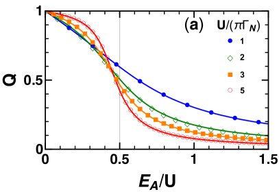
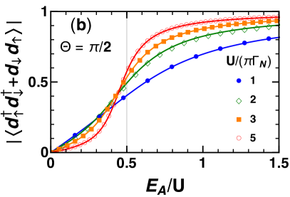
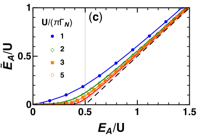
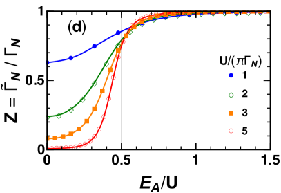
Figure 3: Renormalized parameters plotted vs $E_{A}/U$ for $U/(\pi\Gamma_{N})=1.0$, $2.0$, $3.0$, $5.0$ at $b=0$. (a): Occupation number of Bogoliubov particles $Q$ ($=2\delta/\pi$). (b): Pair correlation $|\bigl{\langle}d^{\dagger}_{\uparrow}d^{\dagger}_{\downarrow}+d_{\downarrow}d_{\uparrow}\bigr{\rangle}|$. (c): Renormalized Andreev-resonance energy $\widetilde{E}_{A}$. (d): Renormalization factor $Z=\widetilde{\Gamma}_{N}/\Gamma_{N}$, which at $E_{A}=0$ takes the values $0.629$, $0.239$, $0.080$, $0.008$, respectively, for the above four values of $U$. Note that $\langle n_{d}\rangle=1.0$ and $|\bigl{\langle}d^{\dagger}_{\uparrow}d^{\dagger}_{\downarrow}+d_{\downarrow}d_{\uparrow}\bigr{\rangle}|=1-Q$, at $\Theta=\pi/2$ along the $\Gamma_{S}$ axis of Fig. 2. The dashed line in (c) denotes the Hartree-Fock energy shift $E_{A}^{\mathrm{HF}}\xrightarrow{E_{A}\gg U/2}E_{A}-U/2$, given in Eq. (41).

IV.1 Ground state properties at $\Theta=\pi/2$

We next consider how the ground state of $H_{\mathrm{eff}}$ evolves as $E_{A}$ varies along the radial direction in the $\xi_{d}$ vs $\Gamma_{S}$ plane, shown in Fig. 2. Note that the eigenstates and eigenvalues of the effective Hamiltonian defined in Eq. (8) do not depend on the angular coordinate $\Theta$.

Figure 3(a) shows the occupation number $Q$ as a function of $E_{A}$ for $U/(\pi\Gamma_{N})=1.0$, $2.0$, $3.0$, and $5.0$. We see that $Q$ decreases as $E_{A}$ increases, especially near $E_{A}\simeq U/2$, where the crossover from the Kondo regime to the valence-fluctuation regime of Bogoliubov particles occurs for large interactions $U/(\pi\Gamma_{N})\gtrsim 2.0$. Figure 3(b) shows the magnitude of the pair correlation function for $\Theta=\pi/2$, where the absolute value is given by $|\bigl{\langle}d^{\dagger}_{\uparrow}d^{\dagger}_{\downarrow}+d_{\downarrow}d_{\uparrow}\bigr{\rangle}|=1-Q$. It increases significantly at $E_{A}\simeq U/2$, i.e., near the quarter-filling point $Q=0.5$ ($\delta=\pi/4$) of Bogoliubov particles, and it saturates to the upper-bound value $1.0$ as $E_{A}$ increases further towards the empty-orbital regime.

The Kondo behaviors of Bogoliubov particles are clearly seen for the renormalized Andreev level $\widetilde{E}_{A}$ and the wave-function renormalization factor $Z=\widetilde{\Gamma}_{N}/\Gamma_{N}$, plotted in Figs. 3(c) and 3(d), respectively. The renormalized level is almost locked at the Fermi level $\widetilde{E}_{A}\simeq 0.0$, for large interactions $U/(\pi\Gamma_{N})\gtrsim 2.0$, over a wide Kondo-dominated region $0\leq E_{A}\lesssim U/2$, taking place the inside of the semicircle in Fig. 2. Correspondingly, the renormalization factor $Z$ is significantly suppressed in this region, and it indicates the fact that the Kondo energy scale $T^{*}$,

$$T^{*}\,\equiv\,\frac{Z}{4\rho_{d}}\,,\qquad\qquad\rho_{d}\,=\,\frac{\sin^{2}\delta}{\pi\Gamma_{N}}\,,$$ (40)

becomes much smaller than the bare tunneling energy scale $\Gamma_{N}$.

In contrast, at $E_{A}\gtrsim U/2$, i.e., in the valence-fluctuation or empty-orbital regime for Bogoliubov particles, the effects of electron correlations become less important: the renormalization factor approaches $Z\simeq 1.0$ and the renormalized level $\widetilde{E}_{A,\sigma}$ approaches the Hartree-Fock (HF) energy shift:

$$E_{A,\sigma}^{\mathrm{HF}}\,\equiv\,E_{A}-\sigma b\,+\,U\left(Q_{\overline{\sigma}}-\frac{1}{2}\right)$$ (41)

$$\ \ \xrightarrow{\,E_{A}\gg U/2,\,b=0\,}\,E_{A}\,-\,\frac{U}{2}\,,$$

since $\,Q_{\overline{\sigma}}\simeq 0.0$ at $E_{A}\gg U/2$ and $b=0$.

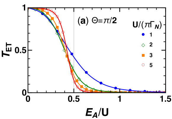
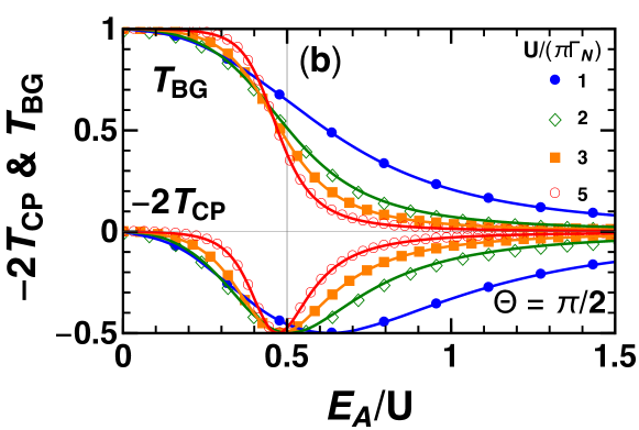
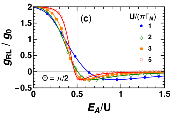
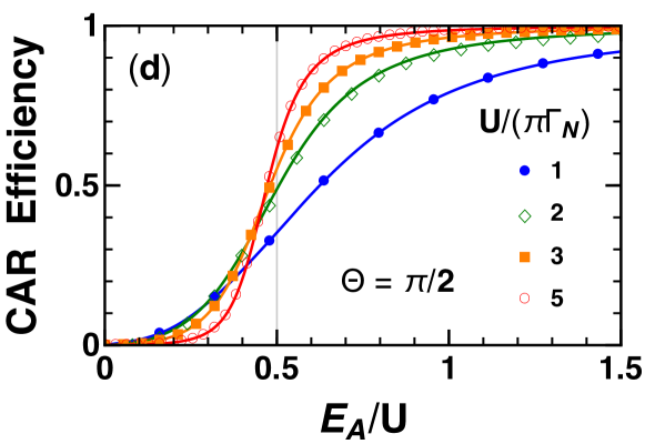
Figure 4: Transport coefficients plotted vs $E_{A}/U$ for $U/(\pi\Gamma_{N})=1.0$, $2.0$, $3.0$, $5.0$ at $b=0$, keeping the Bogoliubov angle fixed at $\Theta=\pi/2$ (i.e., $\xi_{d}=0$). (a): Single-electron transmission $\mathcal{T}_{\mathrm{ET}}$, defined in Eq.  (26). (b): Cooper-pair contributions $-2\mathcal{T}_{\mathrm{CP}}$ ($<0$) and the Bogoliubov-particle transmission $\mathcal{T}_{\mathrm{BG}}=\sin^{2}\delta$, defined in Eqs.  (27) and (28), respectively. (c): Nonlocal conductance $g_{\mathrm{RL}}/g_{0}=2(\mathcal{T}_{\mathrm{BG}}-2\mathcal{T}_{\mathrm{CP}})$ with $g_{0}=\frac{e^{2}}{h}{4\Gamma_{R}\Gamma_{L}}/{\Gamma_{N}^{2}}$. (d): CAR efficiency $\eta_{\text{CAR}}$ defined in Eq. (30).

IV.2 Transport properties at $\Theta=\pi/2$

We next discuss the transport properties. Specifically, in this subsection, we consider the case $\Theta=\pi/2$, where $\xi_{d}=0$ and the occupation number of impurity electrons is fixed at $\langle n_{d}\rangle=1$, reflecting the electron-hole symmetry of $H_{\mathrm{eff}}$ defined in Eq. (50). In this case, the Andreev level takes the value $E_{A}=\Gamma_{S}$, which is determined solely by the coupling strength between the QD and the SC lead and it breaks the particle-hole symmetry of the Bogoliubov particles even at $\xi_{d}=0$.

The transmission probability $\mathcal{T}_{\mathrm{ET}}$ of the single-electron tunneling process is shown in Fig. 4(a). We see that the plateau of the unitary limit $\mathcal{T}_{\mathrm{ET}}\simeq 1.0$ evolves at $0\leq E_{A}\lesssim U/2$, for large $U$. Since $\mathcal{T}_{\mathrm{ET}}=\mathcal{T}_{\mathrm{BG}}-\mathcal{T}_{\mathrm{CP}}$ due to the optical theorem mentioned above, it is the Bogoliubov-particle part $\mathcal{T}_{\mathrm{BG}}=\sin^{2}\delta$ that shows the genuine Kondo ridge, as demonstrated in Fig. 4(b). The single-particle contribution $\mathcal{T}_{\mathrm{ET}}$ decreases outside of the Kondo regime $E_{A}\gtrsim U/2$, at which the occupation number $Q$ of Bogoliubov particles rapidly decreases and the SC pair correlation increases, as demonstrated in Figs. 3(a) and 3(b).

The Cooper-pair contribution $\mathcal{T}_{\mathrm{CP}}$ is also plotted in Fig. 4(b), choosing the Bogoliubov angle to be $\Theta=\pi/2$ and multiplying a factor of $-2$ which emerges for the nonlocal conductance $g_{\mathrm{RL}}\propto\mathcal{T}_{\mathrm{BG}}-2\mathcal{T}_{\mathrm{CP}}$: the negative sign represents the fact that the crossed Andreev reflection induces the counterflow, flowing from the right lead towards the QD. In this case, Eq. (36) can be rewritten further into a similar form to the current noise of normal electrons: $\mathcal{T}_{\mathrm{CP}}=\sin^{2}\delta\,(1-\sin^{2}\delta)$. Blanter and Büttiker (2000); Oguri et al. (2022) Thus, the contribution of $\mathcal{T}_{\mathrm{CP}}$ to the nonlocal conductance is maximized in the case at which the phase shift becomes $\delta=\pi/4$ and it reaches the value $-2\mathcal{T}_{\mathrm{CP}}=-\frac{1}{2}$. The corresponding dip emerges in Fig. 4(b) at the crossover region $E_{A}\simeq U/2$, the width of which becomes of the order of $\Gamma_{N}$.

Figure 4(c) shows the nonlocal conductance, which takes the form $g_{\mathrm{RL}}/g_{0}=-2\sin^{2}\delta\cos 2\delta$ at $\Theta=\pi/2$, as mentioned. It decreases from the unitary-limit value $g_{\mathrm{RL}}/g_{0}=1$ as $E_{A}$ deviates from $E_{A}=0$, and vanishes $g_{\mathrm{RL}}=0$ at $E_{A}\simeq U/2$ where the phase shift reaches $\delta=\pi/4$. The nonlocal conductance becomes negative $g_{\mathrm{RL}}<0$ at $E_{A}\gtrsim U/2$ as the CAR contributions dominate in this region. In particular, it has a dip of the depth $g_{\mathrm{RL}}/g_{0}=-1/4$ at the point where the phase shift takes the value $\delta=\pi/6$.

Similarly, the CAR efficiency takes a simplified form $\eta_{\text{CAR}}=\cos^{2}\delta$ at $\Theta=\pi/2$, and the NRG results are plotted in Fig. 4(d). The efficiency $\eta_{\text{CAR}}$ increases with $E_{A}$, and reaches $\eta_{\text{CAR}}=0.5$ at $\delta=\pi/4$ where $-2\mathcal{T}_{\mathrm{CP}}$ has the dip of the depth $-1/2$ seen in Fig. 4(b). The transient region of $\eta_{\text{CAR}}$ varying from 0 to 1 is estimated to be of the order of $\Gamma_{N}$. Furthermore, at $E_{A}\gg U/2$, the efficiency approaches the saturation value $\eta_{\text{CAR}}=1.0$ although the conductance $g_{\mathrm{RL}}$ itself becomes very small.

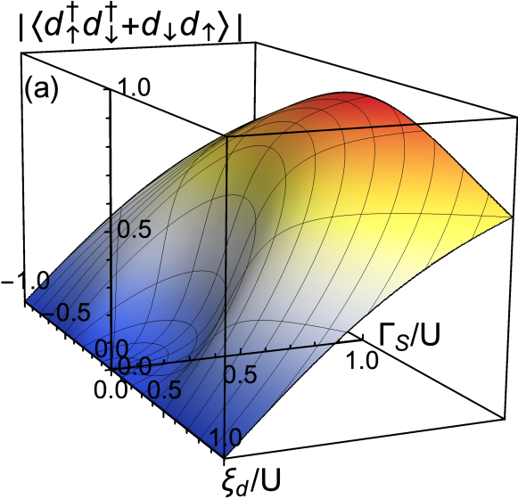
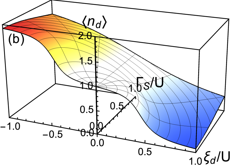
Figure 5: Three-dimensional plots of (a) $|\bigl{\langle}d^{\dagger}_{\uparrow}d^{\dagger}_{\downarrow}+d_{\downarrow}d_{\uparrow}\bigr{\rangle}|$ and (b) $\left\langle n_{d}\right\rangle$, described as functions of $\xi_{d}$ and $\Gamma_{S}$, choosing $U/(\pi\Gamma_{N})=5.0$. Mesh lines are drawn along the polar coordinate ($E_{A}$, $\Theta$), with $E_{A}=\sqrt{\xi_{d}^{2}+\Gamma_{S}^{2}}$ and $\Theta=\tan^{-1}(\Gamma_{S}/\xi_{d})$.

IV.3 The characteristics of CAR along the
polar coordinates $E_{A}$ and $\Theta$ at $b=0$

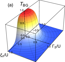
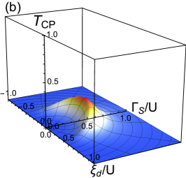
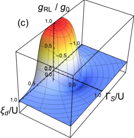
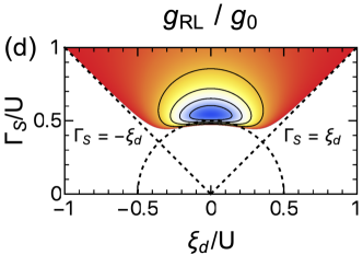
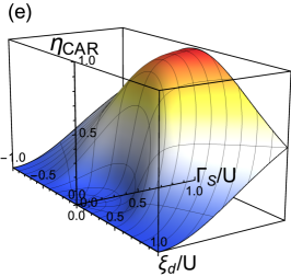
Figure 6: Transport coefficients (a) $\mathcal{T}_{\mathrm{BG}}$, (b) $\mathcal{T}_{\mathrm{CP}}$, (c) $g_{\mathrm{RL}}$, and (e) the CAR efficiency $\eta_{\text{CAR}}$ plotted as functions of $\xi_{d}$ and $\Gamma_{S}$, for $U/(\pi\Gamma_{N})=5.0$ and $b=0$. For these three-dimensional plots, mesh lines are drawn along the polar coordinate ($E_{A}$, $\Theta$). Two-dimensional plot (d) is a contour map for the region where the nonlocal conductance $g_{\mathrm{RL}}$ becomes negative: contour lines are drawn with $0.05$ increments. The CAR dominates $g_{\mathrm{RL}}$ over the parameter region $\Gamma_{S}\gtrsim U/2$ and $\pi/4<\Theta<3\pi/4$, i.e., $\Gamma_{S}>|\xi_{d}|$.

So far, we have discussed the transport properties at $\Theta=\pi/2$, along the vertical $\Gamma_{S}$ axis in the $\xi_{d}$ vs $\Gamma_{S}$ plane. As $\xi_{d}$ varies from the electron-hole symmetric point $\xi_{d}=0$, the Bogoliubov angle $\Theta$ deviates from $\pi/2$. Here we discuss how the ground-state and transport properties vary along the angular direction over the range $0\leq\Theta\leq\pi$.

Figures 5 and 6 show the NRG results of the renormalized parameters and the transport coefficients as functions of $\xi_{d}$ and $\Gamma_{S}$ for a relatively large Coulomb interaction $U/(\pi\Gamma_{N})=5.0$. In these three-dimensional plots, mesh lines are drawn along the polar coordinates $(E_{A},\Theta)$. Note that the superconducting coherence factors, $\cos\Theta$ and $\sin\Theta$, vary in the angular direction: Cooper pairs are strongly entangled at $\pi/2$ and the SC proximity effect becomes weak as $\Theta$ deviates towards $0$ or $\pi$. In contrast, along the radial direction, the crossover between the Kondo regime and valence fluctuation regime of the Bogoliubov particles occurs near the semicircle of radius $E_{A}=U/2$, as mentioned.

IV.3.1 $\Theta$ dependence of $\,\bigl{\langle}d^{\dagger}_{\uparrow}d^{\dagger}_{\downarrow}+d_{\downarrow}d_{\uparrow}\bigr{\rangle}$ and $\,\langle n_{d}\rangle$

Among the renormalized parameters plotted in Fig. 3, the following three, $Q$, $Z$, and $\widetilde{E}_{A}$ do not depend on the Bogoliubov angle $\Theta$, and thus Figs. 3(a), 3(c), and 3(d) remain unchanged as angle $\Theta$ varies. In contrast, the correlation functions which are defined with respect to electrons, such as $|\bigl{\langle}d^{\dagger}_{\uparrow}d^{\dagger}_{\downarrow}+d_{\downarrow}d_{\uparrow}\bigr{\rangle}|=(1-Q)\sin\Theta$ and $\langle n_{d}\rangle=1+(Q-1)\cos\Theta$, evolve with the Bogoliubov angle $\Theta$.

We can see in Fig. 5 (a) that the pair correlation is suppressed due to the Kondo effect at $E_{A}\lesssim U/2$, especially along the valley at $\Theta=\pi/2$, inside the semicircle shown in Fig. 2. The slope from the valley bottom towards the direction parallel to the $\xi_{d}$-axis is suppressed by the coherence factor $\sin\Theta$. Correspondingly, in Fig. 5(b), the occupation number $\langle n_{d}\rangle$ of electrons clearly shows a plateau of a semicircle shape which spreads around the origin $E_{A}=0.0$ of the $\xi_{d}$ vs $\Gamma_{S}$ plane. Note that the occupation number is locked exactly at $\langle n_{d}\rangle=1.0$ along the $\Gamma_{S}$ axis. Outside the plateau $E_{A}\gtrsim U/2$, the superconducting proximity effects dominate over the angular range of $\pi/4<\Theta<3\pi/4$, or equivalently at $\Gamma_{S}>|\xi_{d}|$. In particular, the ridge of the pair correlation develops at $\Theta=\pi/2$, along the $\Gamma_{S}$-axis in Fig. 5(a).

IV.3.2 $\Theta$ dependence of transport properties

Figure 6(a) shows the NRG results of transmission probability of Bogoliubov particles $\mathcal{T}_{\mathrm{BG}}=\sin^{2}\delta$ calculated for $U/(\pi\Gamma_{N})=5.0$. It has an isotropic structure independent of $\Theta$. In particular, the semi-cylindrical elevation of the height $\mathcal{T}_{\mathrm{BG}}\simeq 1.0$ at $E_{A}\lesssim 0.5U$ corresponds to a rotating body of the Kondo ridge shown in Fig. 4 (b). On the slopes of this semicylindrical hill at $E_{A}\simeq 0.5U$, it spreads over the valence fluctuation region of the Bogoliubov particles, at which the transmission probability $\mathcal{T}_{\mathrm{BG}}$ rapidly decreases.

Figure 6(b) shows the transmission probability of Cooper pairs $\mathcal{T}_{\mathrm{CP}}=(1/4)\sin^{2}\Theta\,\sin^{2}2\delta$. It is enhanced along the ridge of a crescent shape that is spreading over the angular range of $\pi/4<\Theta<3\pi/4$ (at which $\Gamma_{S}>|\xi_{d}|$) on the arc of radius $E_{A}\simeq U/2$, where the crossover between the Kondo-singlet and the superconducting-singlet states takes place. The ridge height of $\mathcal{T}_{\mathrm{CP}}$ decreases from the maximum value $0.25$ as $\Theta$ deviates from $\Theta=\pi/2$, showing the $\sin^{2}\Theta$ dependence. The width of the crescent region in the radial direction is of the order of $\Gamma_{N}$ ($\simeq 0.06U$ in Fig. 6(b) ).

The nonlocal conductance $g_{\mathrm{RL}}/g_{0}=2(\mathcal{T}_{\mathrm{BG}}-2\mathcal{T}_{\mathrm{CP}})$ is shown in Fig. 6(c). It also features a flat-topped semicylindrical elevation at $E_{A}\lesssim U/2$, which is mainly due to the contributions of the Bogoliubov-particle part $\mathcal{T}_{\mathrm{BG}}$ seen in Fig. 6(a). The nonlocal conductance $g_{\mathrm{RL}}$ becomes negative at the foot of the hill, specifically at $E_{A}\gtrsim U/2$ along the arc of the range $\pi/4<\Theta<3\pi/4$, where the CAR dominates the transport. In order to see more precisely the profile of the negative-conductance region, a contour plot of $g_{\mathrm{RL}}$ is shown in Fig. 6(d). The dip in the profile becomes deepest at $\Theta=\pi/2$ and $E_{A}/U\simeq 0.55$, as seen also in Fig. 4(c). The behavior of $g_{\mathrm{RL}}$ along the $\Theta$ direction is determined by the coherence factor $\sin^{2}\Theta$ of the Cooper-pair part $\mathcal{T}_{\mathrm{CP}}$ in Eq. (36). It suppresses the CAR contributions to the nonlocal conductance as $\Theta$ deviates from $\pi/2$. The crescent-shaped dip emerged for $g_{\mathrm{RL}}$ reflecting the corresponding one seen in Fig. 6(b) for $\mathcal{T}_{\mathrm{CP}}$, and the dip spreads from $E_{A}\simeq U/2$ to $E_{A}\sim U/2+\Gamma_{N}$ in the direction of the $\Gamma_{S}$-axis. These results suggest that the crescent dip region will be a plausible target to probe the CAR contributions in experiments.

The NRG result of the CAR efficiency at $b=0$, $\eta_{\text{CAR}}=\sin^{2}\Theta\,\cos^{2}\delta$, is shown in Fig. 6(e). We can see that its behavior is similar to that of the pair correlation described in Fig. 5(a): the ridge of $\eta_{\text{CAR}}$ evolves at $E_{A}\gtrsim U/2$ in the direction of $\Theta=\pi/2$ along the $\Gamma_{S}$ axis. In the valley region at $E_{A}\lesssim U/2$, however, the slope of $\eta_{\text{CAR}}$ in the direction parallel to the $\xi_{d}$ axis becomes steeper as it is determined by the coherence factor $\sin^{2}\Theta$, whereas that for the pair correlation function is $\sin\Theta$. There are also some quantitative differences between the profiles of the CAR efficiency and the pair correlation function in the radial direction: it is because $\eta_{\text{CAR}}\propto\cos^{2}\delta$, whereas $|\bigl{\langle}d^{\dagger}_{\uparrow}d^{\dagger}_{\downarrow}+d_{\downarrow}d_{\uparrow}\bigr{\rangle}|\propto 1-2\delta/\pi$.

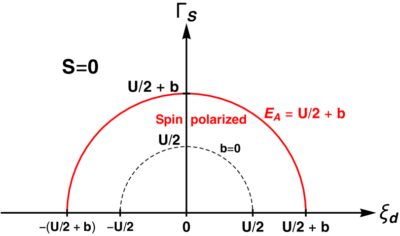
Figure 7: Parameter space of $H_{\mathrm{eff}}$ at finite magnetic fields. Near the semicircle of radius $E_{A}=U/2+b$ with $E_{A}=\sqrt{\xi_{d}^{2}+\Gamma_{S}^{2}}$, the occupation number of the Bogoliubov particles in the Andreev level varies rapidly from $Q\simeq 1.0$ to $Q\simeq 0.0$ for large $U$. Specifically, in the atomic limit $\Gamma_{N}\to 0$, the ground state is spin polarized $Q_{\uparrow}\to 1.0$ inside the semicircle at finite fields $b\neq 0$. The Andreev scattering can dominate the transport in the range of $\pi/4<\Theta<3\pi/4$ outside the semicircle which evolves with $b$.

V Crossed-Andreev transport at finite magnetic fields $b\neq 0$

Both the Kondo effect and the superconducting proximity effect are sensitive to a magnetic field. Here we study precisely how the CAR contributions vary at finite magnetic fields.

Figure 7 shows the parameter space of the effective Hamiltonian $H_{\mathrm{eff}}$ at finite magnetic fields ($b>0$). In the atomic limit $\Gamma_{N}\to 0$, the phase boundary evolves with $b$, and the ground state of the isolated QD is spin polarized inside the semicircle of radius $E_{A}=U/2+b$ where the Andreev level is occupied by a single Bogoliubov particle with majority spin: $Q_{\uparrow}\to 1.0$. In contrast, outside the semicircle, the Andreev level is empty $Q=0$ and the ground state is unpolarized. The transition is caused by the level crossing between the energy level $E_{A,\uparrow}\equiv E_{A}-b$ of the singly occupied majority-spin state and the spin-singlet empty state of energy $U/2$, and thus it takes place at the circumference of the semicircle $E_{A,\uparrow}=U/2$.

The level crossing becomes a gradual crossover, the width of which is of the order of $\Gamma_{N}$, when normal leads are connected. The CAR contribution to the nonlocal conductance is enhanced also at finite $b$ near the crossover region: specifically along the circumference of radius $E_{A}\simeq U/2+b$ over the angular range of $\pi/4\lesssim\Theta\lesssim 3\pi/4$. We will consider magnetic-field dependence of the CAR contribution precisely in this section.

V.1 Ground-state and transport properties at $\Theta=\pi/2$

At finite magnetic fields, the renormalized parameters become dependent on spin components $\sigma$ and vary as Zeeman splitting increases. Our discussions in the following are based on the transport formulas for the ground state given in Eqs. (26)–(30). The NRG calculations have been carried out for a strong interaction $U/(\pi\Gamma_{N})=5.0$ in order to clarify how the electron correlations affect the crossed Andreev reflection in the multiterminal network.

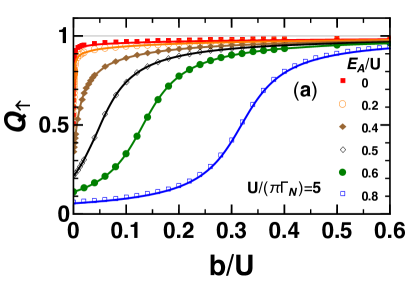
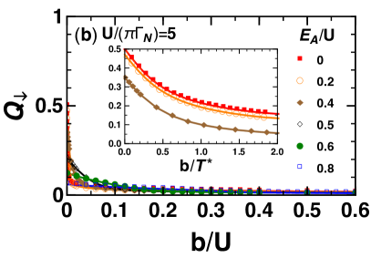
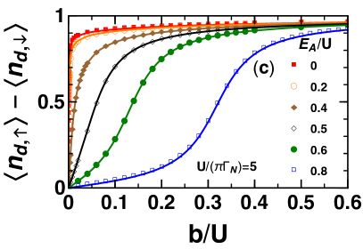
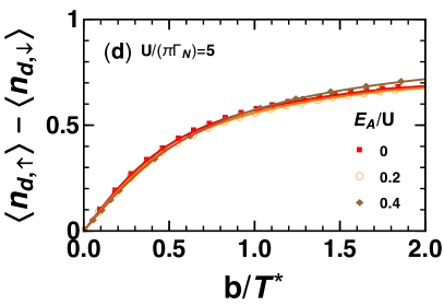
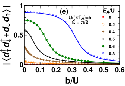
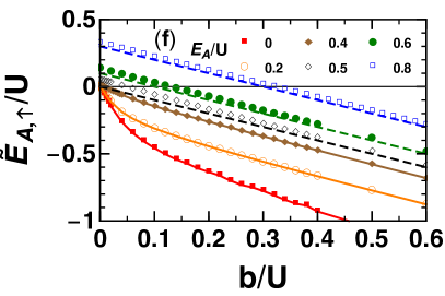
Figure 8: Magnetic-field dependence of the renormalized parameters calculated at different Andreev-level positions $E_{A}/U=0.0$, $0.2$, $0.4$, $0.5$, $0.6$, and $0.8$, for a fixed interaction $U/(\pi\Gamma_{N})=5.0$. (a), (b) Occupation number of Bogoliubov particles $Q_{\uparrow}$ and $Q_{\downarrow}$. Inset in (b) is an enlarged plot of $Q_{\downarrow}$ vs $b/T^{*}$, with $T^{*}$ the characteristic energy scale of the Kondo regime defined at $b=0$ in Eq. (40). For $E_{A}=0.0$, $0.2U$, and $0.4U$, it takes the value $T^{*}/(\pi\Gamma_{N})=0.002$, $0.005$, and $0.097$, respectively (or $T^{*}/U=0.0004$, $0.001$, and $0.019$). The values of $Z=\widetilde{\Gamma}_{N}/\Gamma_{N}$ at these three points of $E_{A}$ are given by $Z=0.008$, $0.02$, $0.31$, respectively. (c) Magnetization $m_{d}=\langle n_{d\uparrow}\rangle-\langle n_{d\downarrow}\rangle$, which does not depend on the Bogoliubov angle $\Theta$. (d) Enlarged view of $m_{d}$ for $E_{A}=0.0$, $0.2U$, and $0.4U$ plotted vs $b/T^{*}$ in the Kondo regime. (e) Pair correlation $|\bigl{\langle}d^{\dagger}_{\uparrow}d^{\dagger}_{\downarrow}+d_{\downarrow}d_{\uparrow}\bigr{\rangle}|$ at $\Theta=\pi/2$, which in this case is given by $1-Q$ and varies with $b$ and $E_{A}$, in contrast to the electron filling $\langle n_{d}\rangle\equiv 1.0$ that remains unchanged along the $\Gamma_{S}$ axis at $\xi_{d}=0$. (f) Renormalized Andreev levels $\widetilde{E}_{A,\uparrow}$. The dashed straight lines represent the Hartree-Fock (HF) result $E_{A}^{\mathrm{HF}}\xrightarrow{\,E_{A}\gg U/2\,}E_{A}-U/2-b$.

V.1.1 $b$ dependence of renormalized parameters

Figures 8(a)–8(f) show the magnetic-field dependence of the renormalized parameters, calculated for several different positions of the Andreev level: $E_{A}/U=0.0$, $0.2$, $0.4$, $0.5$, $0.6$, and $0.8$. The results commonly reflect the Fermi-liquid properties of the Bogoliubov particles, which evolve as $E_{A}$ and $b$ vary.

For $0\leq E_{A}\lesssim U/2$, the renormalized parameters exhibit a universal $b/T^{*}$ scaling behavior at small magnetic fields, with $T^{*}$ the Kondo energy scale defined at zero field $b=0$ by Eq. (40). The magnitude of $T^{*}$ depends sensitively on the interaction strength and the level position $E_{A}$, and, for instance, for $U/(\pi\Gamma_{N})=5.0$, it is given by $T^{*}/(\pi\Gamma_{N})=0.002$, $0.005$, and $0.097$ for $E_{A}/U=0.0$, $0.2$, and $0.4$, respectively. At the magnetic field of order at $b\sim T^{*}$, the Kondo resonance of Bogoliubov particles splits into two as the Zeeman effect dominates. In contrast, in the parameter region of $E_{A}\gtrsim U/2$ where the Andreev level deviates further from the Fermi level, the renormalization effects due to the electron correlations are suppressed, and the low-energy states depend significantly on whether $U/2\lesssim E_{A}\lesssim U/2+b$ or $U/2+b\lesssim E_{A}$. The magnetization $m_{d}$ of quantum dot is almost fully polarized at $U/2\lesssim E_{A}\lesssim U/2+b$, where the Zeeman effect dominates. In contrast, the superconducting proximity effect dominates outside the semicircle of radius $E_{A}\gtrsim U/2+b$ in the angular range of $\pi/4<\Theta<3\pi/4$. We will discuss these of variations of the ground state properties in more detail in the following.

Figures 8(a)–8(d) describe the occupation number $Q_{\sigma}$ and the magnetization $m_{d}\equiv\langle n_{d\uparrow}\rangle-\langle n_{d\downarrow}\rangle$ as functions of magnetic fields. Note that two of them, Fig. 8(d) and the inset presented for $Q_{\downarrow}$ in Fig. 8(b), are plotted vs $b/T^{*}$ for small magnetic fields. We see in Fig. 8(d) that the magnetization $m_{d}$ for $E_{A}/U\lesssim 0.4$ exhibits the universal Kondo scaling behavior at $b\lesssim T^{*}$. It can also be recognized that the three curves for $Q_{\downarrow}$ shown in the inset in Fig. 8(b) will collapse into a single universal curve if we introduce the offset values along the vertical axis which is determined at $b=0$ for each $E_{A}$: note that the occupation number takes the value $Q_{\sigma}=0.5$ at $E_{A}=b=0$.

However, as seen in Figs. 8(a) and 8(c), the Zeeman effect dominates at strong magnetic fields. Note that the magnetization can also be written as $m_{d}=Q_{\uparrow}-Q_{\downarrow}$ and does not depend on the Bogoliubov angle $\Theta$. The Kondo behavior disappears for $E_{A}/U\gtrsim 0.5$, at which the Bogoliubov particles are in the valence fluctuation or empty orbital regime at $b=0$. In this region of $E_{A}/U$, the occupation number $Q_{\uparrow}$ of the majority-spin component and the magnetization $m_{d}$ show a steep increase at magnetic fields of $b\simeq E_{A}-U/2$ where the level crossing occurs. As magnetic field increases further $b\gtrsim E_{A}-U/2$, the magnetization rapidly approaches the saturation value $m_{d}\to 1.0$.

Figure 8(e) shows the magnetic-field dependence of the SC pair correlation function $|\bigl{\langle}d^{\dagger}_{\uparrow}d^{\dagger}_{\downarrow}+d_{\downarrow}d_{\uparrow}\bigr{\rangle}|$ which becomes equal to $1-Q$ in the direction of $\Theta=\pi/2$. While the pair correlation increases with $E_{A}$, it decreases as $b$ increases. We can see that the SC proximity effect dominates at small fields $b\lesssim E_{A}-U/2$ in the parameter region of $E_{A}\gtrsim U/2$, i.e, the outside of the semicircle of radius $E_{A}\gtrsim U/2+b$ shown in Fig. 7. In this region, the SC pair correlation function can take the value of the order of 10% of the maximum possible value $|\bigl{\langle}d^{\dagger}_{\uparrow}d^{\dagger}_{\downarrow}+d_{\downarrow}d_{\uparrow}\bigr{\rangle}|=1$, as seen in Fig.8(e) at magnetic fields of the order of $b\sim 0.1U$. However, as magnetic field approaches $b\simeq E_{A}-U/2$, the crossover to the Zeeman-dominated spin-polarized regime occurs, and the pair correlation rapidly decreases. The sum of the phase shifts takes the value $\delta_{\uparrow}+\delta_{\downarrow}\simeq\pi/2$ in the crossover region. Therefore, the Andreev scattering is most enhanced at this point since the factor $\sin^{2}(\delta_{\uparrow}+\delta_{\downarrow})$ that determines $\mathcal{T}_{\mathrm{CP}}$ takes the maximum value.

Figure 8(f) shows the results for the majority-spin component of the renormalized Andreev level $\widetilde{E}_{A,\uparrow}$ which includes the Zeeman energy and the many-body corrections defined in Eq. (17). For $E_{A}\lesssim U/2$, the slope of $\widetilde{E}_{A,\uparrow}$ is steep at small magnetic fields $b\simeq 0$. This is because the spin susceptibility, $\chi_{s}=m_{d}/b$, is enhanced in this region by the Kondo effect as seen in Fig. 8(c). The slope becomes gradual, however, as $b$ increases and the crossover to the Zeeman-dominated regime occurs at $b\sim T^{*}$. In contrast, for $E_{A}\gtrsim U/2$, the renormalized level $\widetilde{E}_{A,\uparrow}$ at small magnetic fields $b\simeq 0$ shifts away from the Fermi level, and the occupation number of the Bogoliubov particles $Q$ decreases as $E_{A}$ increases. However, as magnetic field increases further, the renormalized level $\widetilde{E}_{A,\uparrow}$ crosses the Fermi level at $b\simeq E_{A}-U/2$, and the occupation number of the majority spin component $Q_{\uparrow}$ increases abruptly at the crossing point. The dashed straight lines in Fig. 8(f) represent the Hartree-Fock energy shift $E_{A,\uparrow}^{\mathrm{HF}}$, which asymptotically takes the following form at $E_{A}\gg U/2$:

$$E_{A,\uparrow}^{\mathrm{HF}}\,\equiv\,E_{A}-b\,+\,U\left(Q_{\downarrow}-\frac{1}{2}\right)$$

$$\ \ \xrightarrow{\,E_{A}\gg U/2\,}\,E_{A}-\frac{U}{2}-b\,.$$ (42)

The NRG results for $\widetilde{E}_{A,\uparrow}$ and the Hartree-Fock energy shifts show a close agreement for $E_{A}\gtrsim U/2$. This is caused by the fact that the renormalization factor approaches $Z_{\sigma}\simeq 1.0$ and it becomes less important at the crossover region between the Zeeman-dominated spin-polarized regime and the SC-dominated regime.

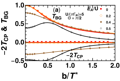
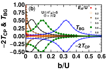
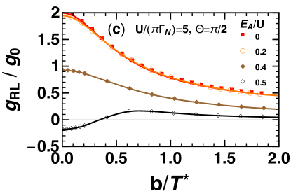
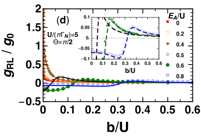
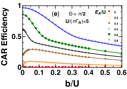
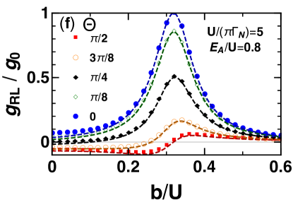
Figure 9: Magnetic-field dependence of the transport coefficients at $\Theta=\pi/2$ for different positions of $E_{A}/U=0$, $0.2$, $0.4$, $0.5$, $0.6$, and $0.8$, for a strong interaction $U/(\pi\Gamma_{N})=5.0$. Top panel describes $\mathcal{T}_{\mathrm{BG}}=\sum_{\sigma}\sin^{2}{\delta_{\sigma}}/2$, and $\Theta$ dependent part $-2\mathcal{T}_{\mathrm{CP}}$ for (a) small $E_{A}\lesssim 0.5U$ and (b) large $E_{A}\gtrsim 0.5U$. (c), (d) Nonlocal conductance $g_{\mathrm{RL}}/g_{0}$. Inset in (d) is an enlarged view in the region around $g_{\mathrm{RL}}/g_{0}\approx 0.0$: the dashed lines represent the perturbation results obtained with Eq. (43). The characteristic energy is given by $T^{*}/U=0.0004$, $0.001$, $0.019$, and 0.097 for $E_{A}/U=0.0$, $0.2$, $0.4$, and $0.5$, respectively. (e) CAR efficiency $\eta_{\text{CAR}}$. (f) $g_{\mathrm{RL}}/g_{0}$ at a fixed Andreev level position $E_{A}=0.8U$ for several different angles $\Theta=0$, $\pi/8$, $\pi/4$, $3\pi/8$, $\pi/2$: the dashed lines here also represent the perturbation results.

V.1.2 $b$ dependence of transport properties at $\Theta=\pi/2$

We next discuss the magnetic-field dependence of transport coefficients in the direction of $\Theta=\pi/2$, i.e., along the $\Gamma_{S}$ axis ($\xi_{d}=0$). The NRG results are shown in Fig. 9: the magnetic field $b$ is scaled by $T^{*}$ in two of the panels 9(a) and 9(c), whereas the other panels are plotted vs $b/U$.

We see in Fig. 9(a) that the transmission probabilities of Bogoliubov particles $\mathcal{T}_{\mathrm{BG}}$ for $E_{A}\lesssim 0.2U$ collapse into a single curve at small magnetic fields $b\lesssim T^{*}$, showing a universal $b/T^{*}$ Kondo scaling behavior, whereas the probability of the Cooper-pairs $\mathcal{T}_{\mathrm{CP}}$ is suppressed in this region. Correspondingly, the nonlocal conductance $g_{\mathrm{RL}}$ exhibits the scaling behavior for $E_{A}\lesssim 0.2U$, as shown in Fig. 9(c). The results for $\mathcal{T}_{\mathrm{BG}}$ and $g_{\mathrm{RL}}$ at $E_{A}=0.4U$ still show a similar monotonic decrease although they did not collapse into the universal curves. Therefore, the CAR efficiencies $\eta_{\mathrm{CAR}}=\mathcal{T}_{\mathrm{CP}}/\mathcal{T}_{\mathrm{BG}}$ for $E_{A}/U=0.2$ and $0.4$, described in Fig. 9(e), increase clearly with $b$ at small magnetic fields near $b\simeq 0$. It shows that the Zeeman splitting suppresses the Kondo correlations and assists the contributions of the Cooper-pair tunneling.

In contrast, when the Andreev level situates further away from the Fermi level $E_{A}\gtrsim U/2$, the ground state evolves from the superconductivity-dominated regime to the Zeeman dominated spin-polarized regime, as magnetic field increases. In particular, at $b\simeq E_{A}-U/2$, i.e., the crossover region between these two regimes, the transmission probability of the Bogoliubov particles $\mathcal{T}_{\mathrm{BG}}=\left(\sin^{2}\delta_{\uparrow}+\sin^{2}\delta_{\downarrow}\right)/2$ has a peak, which emerges in Fig. 9(b), as the phase shifts take the value $\delta_{\uparrow}\simeq\pi/2$ and $\delta_{\downarrow}\simeq 0$. Similarly, the Cooper-pair contribution $\mathcal{T}_{\mathrm{CP}}=(1/4)\sin^{2}\Theta\,\sin^{2}\bigl{(}\delta_{\uparrow}+\delta_{\downarrow})$ reaches the maximum value $1/4$ at $b\simeq E_{A}-U/2$ in the crossover region. This is consistent with the previous work that examined an N-QD-SC system with the modified second-order perturbation theory. Yamada et al. (2007) It revealed the fact that the Andreev scattering is significantly enhanced under the condition that the renormalized parameters satisfy $\prod_{\sigma}(\widetilde{E}_{A,\sigma}/\widetilde{\Gamma}_{N,\sigma})=1$: this can be rewritten into the form $\cot\delta_{\uparrow}\cot\delta_{\downarrow}=1$ and is fulfilled at $\delta_{\uparrow}+\delta_{\downarrow}=\pi/2$.

We can see in Fig. 9(d) that, for $E_{A}\gtrsim U/2$, the nonlocal conductance $g_{\mathrm{RL}}=\mathcal{T}_{\mathrm{BG}}-2\mathcal{T}_{\mathrm{CP}}$ becomes negative in the SC-dominated regime $b\lesssim E_{A}-U/2$, whereas $g_{\mathrm{RL}}$ takes a positive value in the Zeeman-dominated regime $b\gtrsim E_{A}-U/2$. In particular, for $E_{A}\gtrsim 0.6U$, the nonlocal conductance forms a flat valley structure at $0\leq b\lesssim E_{A}-U/2$ the bottom of which is negative and is less sensitive to $b$. This is caused by the fact that the peak of $\mathcal{T}_{\mathrm{BG}}$ and the dip of $-2\mathcal{T}_{\mathrm{CP}}$ move almost synchronously, in Fig. 9(b), as $E_{A}$ increases from $0.5U$. For observing the flat valley structure of $g_{\mathrm{RL}}$, the depth of which should not be too shallow, and thus $E_{A}-U/2$ should be of the order of $\Gamma_{N}$, or should not be too much larger than $\Gamma_{N}$. Note that, in this magnetic-field region $0\leq b\lesssim E_{A}-U/2$, the occupation number of the Bogoliubov particles with the minority spin is almost empty $Q_{\downarrow}\simeq 0.0$ and the transport coefficients are determined by the majority-spin component $Q_{\uparrow}$. In order to verify this quantitatively, we expand the nonlocal conductance into the following form, keeping the terms up to the first order with respect to $\delta_{\downarrow}$,

$$g_{\mathrm{RL}}\,\approx \ \,g_{0}\Bigl{[}\,\cos^{2}\Theta\,\sin^{2}\delta_{\uparrow}-\delta_{\downarrow}\sin^{2}\Theta\,\sin 2\delta_{\uparrow}\,\Bigr{]}\,+\,O\!\left(\delta_{\downarrow}^{2}\right)$$

$$\xrightarrow{\,\Theta=\frac{\pi}{2}\,} \ g_{0}\,\left[\,-\delta_{\downarrow}\,\sin 2\delta_{\uparrow}\,+\,O\!\left(\delta_{\downarrow}^{2}\right)\,\right]\,.$$ (43)

The dashed lines plotted in the inset of Fig. 9(d) are the results evaluated with Eq. (43), using the NRG results for $\delta_{\sigma}$. These results show close agreement with the full NRG calculations of $g_{\mathrm{RL}}$ plotted with the symbols, i.e., for $E_{A}/U=0.6$ ($\bullet$) and $0.8$ ($\square$).

So far, we have considered behaviors along the angular direction of $\Theta=\pi/2$. Figure 9(f) compares the magnetic-field dependence of $g_{\mathrm{RL}}$ for several different angles $\Theta$, keeping the Andreev-level position at $E_{A}=0.8U$. The dashed lines, which also show nice agreement with the full NRG results (symbols) of $g_{\mathrm{RL}}$ in this figure, are the perturbation results obtained from Eq. (43). We find that the flat structure with negative $g_{\mathrm{RL}}$ remains for $\Theta=3\pi/8$, where the angle largely deviates from $\pi/2$. As $\Theta$ derives further, however, $g_{\mathrm{RL}}$ becomes positive at $0<\Theta<\pi/4$, or $3\pi/4<\Theta<\pi$. Note that the $\Theta$ dependence enters the nonlocal conductance through the coherence factor $\sin^{2}\Theta$ in $\mathcal{T}_{\mathrm{CP}}$, and thus $g_{\mathrm{RL}}$ is symmetrical with respect to the $\Gamma_{S}$-axis in parameter space shown in Fig. 7.

In the SC-dominated regime $0\leq b\lesssim E_{A}-U/2$, both components of the phase shift approach zero as $E_{A}$ increases keeping $b$ unchanged, i.e., $\delta_{\uparrow}\simeq 0$ and $\delta_{\downarrow}\simeq 0$ as seen in Figs. 8(a) and 8(b). The CAR efficiency $\eta_{\mathrm{CAR}}$ is enhanced in this region although it decreases as $b$ increases, as seen in Fig. 9(e) for $E_{A}/U=0.6$ and $0.8$. In particular, for $E_{A}\gg U$, the efficiency approaches saturation value $\eta_{\mathrm{CAR}}\to 1.0$ at small magnetic fields near $b\simeq 0.0$.

V.2 The characteristics of CAR along the
polar coordinates $E_{A}$ and $\Theta$ at $b\neq 0$

In this subsection, we consider the $\Theta$ dependence of the transport properties at finite magnetic fields in more detail. Specifically, in order to clarify in which situations the CAR contribution can dominate the nonlocal conductance by overcoming the disturbance of the SC proximity effects by the Coulomb interaction and magnetic field, we explore a wide range of the parameter space, i.e., the $\xi_{d}$ vs $\Gamma_{S}$ plane. Our discussion here is based on the NRG results in Figs. 10 and 11, obtained for a relatively large interaction $U/(\pi\Gamma_{N})=5.0$: the Kondo temperature in this case is given by $T_{K}/U=0.0004$, which is defined as the value of the characteristic energy scale $T^{\ast}$ at $E_{A}=b=0$. These results can be compared with those for zero field presented in Figs. 5 and 6.

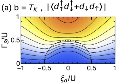
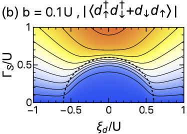
Figure 10: Contour maps of $|\bigl{\langle}d^{\dagger}_{\uparrow}d^{\dagger}_{\downarrow}+d_{\downarrow}d_{\uparrow}\bigr{\rangle}|$ at finite magnetic fields: (a) $b=T_{K}$ and (b) $b=0.1U$, for $U/(\pi\Gamma_{N})=5.0$. Here, $T_{K}=0.0004U$ is defined as the value of $T^{\ast}$ at $E_{A}=b=0$. The contours are drawn with 0.1 increments, and the dashed line represents the semicircle of radius $E_{A}=U/2+b$.

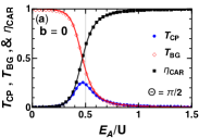
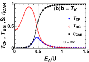
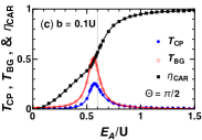
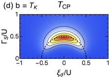
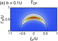
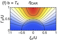
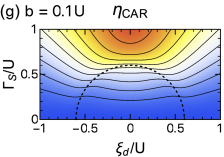
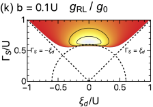
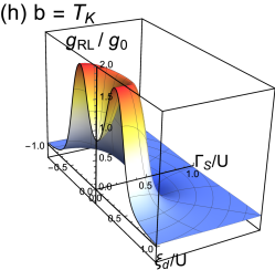
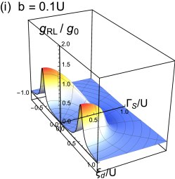
Figure 11: Bogoliubov-angle dependence of transport coefficients in a strong interaction case $U/(\pi\Gamma_{N})=5.0$ at small $b=T_{K}$ and large $b=0.1U$ fields, with $T_{K}/U=0.0004$ defined as the value of $T^{\ast}$ at $E_{A}=b=0$. In the top panels for (a) $b=0$, (b) $b=T_{K}$, and (c) $b=0.1U$, the coefficients $\mathcal{T}_{\mathrm{BG}}$, $\mathcal{T}_{\mathrm{CP}}$, and CAR efficiency $\eta_{\mathrm{CAR}}$ at $\Theta=\pi/2$ are plotted vs $E_{A}/U$. (d), (e) Contour maps of $\mathcal{T}_{\mathrm{CP}}$, drawn with 0.05 increments. (f), (g) Contour maps of $\eta_{\mathrm{CAR}}$, drawn with 0.1 increments. (h)–(k) Nonlocal conductance $g_{\mathrm{RL}}/g_{0}$. In particular, (j) and (k) are the contour maps for negative conductance region $g_{\mathrm{RL}}<0$, for which contours are drawn with $0.05$ increments. The dashed semicircle of radius $E_{A}=b+U/2$ in (d)–(g) and (j)–(k) corresponds to the one in Fig. 7.

V.2.1 $\Theta$ dependence of $\bigl{\langle}d^{\dagger}_{\uparrow}d^{\dagger}_{\downarrow}+d_{\downarrow}d_{\uparrow}\bigr{\rangle}$ at $b\neq 0$

Figure 10 shows the pair correlation $|\bigl{\langle}d^{\dagger}_{\uparrow}d^{\dagger}_{\downarrow}+d_{\downarrow}d_{\uparrow}\bigr{\rangle}|=(1-Q)\sin\Theta$ for two different magnetic-field strengths: (a) $b=T_{K}$ and (b) $b=0.1U$. Here, the occupation number $Q$ of Bogoliubov particles does not depend on $\Theta$ but varies with $b$ and $E_{A}$, as mentioned and shown in Figs. 8(a) and 8(b).

The pair correlation function for a small magnetic field $b=T_{K}$, shown in Fig. 10(a), is enhanced outside the semicircle of radius $E_{A}\gtrsim U/2+b$ in the angular range of $\pi/4<\Theta<3\pi/4$, especially along the $\Gamma_{S}$-axis ($\Theta=\pi/2$), where the SC proximity effects dominate. In contrast, it is suppressed by the Kondo effect inside the semicircle $E_{A}\lesssim U/2+b$. Note that $b$ is much smaller than $U$ in this case ($T_{K}/U=0.0004$).

Figure 10(b) shows the pair correlation function for a large magnetic field $b=0.1U$. Although it is qualitatively similar to Fig. 10(a), we can see that the slope just inside of the circumference becomes steeper than that for $b=T_{K}$. The radius of the dashed semicircle at the crossover region in this case is $E_{A}\simeq U/2+b$ ($=0.6U$), and thus the expansion of the circumference due to $b$ becomes visible in Fig. 10(b).

V.2.2 $\Theta$ dependence of transport properties at $b\neq 0$

The top panels of Fig. 11 show $\mathcal{T}_{\mathrm{BG}}$, $\mathcal{T}_{\mathrm{CP}}$, and $\eta_{\mathrm{CAR}}$ as functions of $E_{A}$ for three different magnetic fields: (a) $b=0$, (b) $b=T_{K}$, and (c) $b=0.1U$, taking the Bogoliubov angle to be $\Theta=\pi/2$, i.e., the direction in which the SC proximity effect is most enhanced. We can see that, as $b$ increases, the peak of the Cooper-pair tunneling part $\mathcal{T}_{\mathrm{CP}}$, emerging at $E_{A}\simeq U/2+b$, moves with the crossover region towards the larger $E_{A}$ side along the horizontal axis. The peak height is $1/4$ and the width becomes of the order of $\Gamma_{N}$ ($\simeq 0.06U$ in this case). The Bogoliubov-particle part $\mathcal{T}_{\mathrm{BG}}$ exhibits the flat Kondo plateau at zero field, plotted in Fig. 11(a) for comparison. However, the Zeeman splitting dominates at magnetic fields of the order of $b\simeq T_{K}$ and the top of the Kondo plateau caves in around $E_{A}\simeq 0.0$, as seen in Fig. 11(b). As magnetic field increases further, the peak of $\mathcal{T}_{\mathrm{BG}}$ in Fig. 11(c) becomes small and approaches the peak of $\mathcal{T}_{\mathrm{CP}}$ that situates close to the crossover region.

The CAR efficiency $\eta_{\mathrm{CAR}}=\mathcal{T}_{\mathrm{CP}}/\mathcal{T}_{\mathrm{BG}}$ plotted in Fig. 11(c) takes relatively large value $0.1\lesssim\eta_{\mathrm{CAR}}\lesssim 0.5$ even at $E_{A}\lesssim U/2+b$. Such a behavior is not seen for small $b$ in Figs. 11(a) and 11(b), and reflects the suppression of $\mathcal{T}_{\mathrm{BG}}$ caused by a large magnetic field $b=0.1U$. Outside the crossover region $E_{A}\gtrsim U/2+b$, however, $\eta_{\mathrm{CAR}}$ shows a similar behavior in Figs. 11(a)–11(c): it approaches the saturation value $\eta_{\mathrm{CAR}}\to 1.0$ as $E_{A}$ increases.

The Bogoliubov angle $\Theta$ enters the nonlocal conductance $g_{\mathrm{RL}}$ through $\mathcal{T}_{\mathrm{CP}}$ since the Bogoliubov part $\mathcal{T}_{\mathrm{BG}}$ is independent of it. Figures 11(d) and 11(e) show the contour maps of $\mathcal{T}_{\mathrm{CP}}$ described on the $\xi_{d}$ vs $\Gamma_{S}$ plane, for magnetic fields of (d) $b=T_{K}$ and (e) $b=0.1U$. The Cooper-pair tunneling part $\mathcal{T}_{\mathrm{CP}}$ is enhanced along in the crescent-shaped region on the arc of radius $E_{A}=U/2+b$ in the angular range of $\pi/4<\Theta<3\pi/4$. The crescent region spreads over the direction of the $\Gamma_{S}$-axis with the width of the order of $\Gamma_{N}$ ($\simeq 0.06U$ in this case). As the magnetic field increases, the crescent region moves upward along the $\Gamma_{S}-$axis, together with the arc indicated as a dashed semicircle in Figs. 11(d) and 11(e). This evolution of the crescent region causes the CAR-dominated flat structure of nonlocal conductance $g_{\mathrm{RL}}$ that emerged in the magnetic-field dependence in Figs. 9(d) and 9(f).

Figures 11(f) and 11(g) show the contour maps of the CAR efficiency $\eta_{\mathrm{CAR}}$ for magnetic fields of (f) $b=T_{K}$ and (g) $b=0.1U$. Figure 11(f) captures the typical profile of $\eta_{\mathrm{CAR}}$ at small fields of order $b\simeq T_{K}$: the CAR efficiency is enhanced in the SC-dominated regime $E_{A}\gtrsim U/2+b$ and $\pi/4<\Theta<3\pi/4$, whereas it decreases rapidly outside this region, especially just inside the semicircle, $E_{A}\lesssim U/2+b$, in the edge of the Zeeman-dominated spin-polarized regime. It reflects the steep slope along the direction of $\Theta=\pi/2$, seen in Fig. 11(b), at the crossover region $E_{A}\simeq U/2+b$. In contrast, at large fields of order $b\simeq 0.1U$, the corresponding slope of $\eta_{\mathrm{CAR}}$ inside the semicircle shows a slow modest decline as seen in Fig. 11(g). This modest decline of $\eta_{\mathrm{CAR}}=\mathcal{T}_{\mathrm{CP}}/\mathcal{T}_{\mathrm{BG}}$ is caused by the behavior of the transmission probability of the Bogoliubov particles in the denominator that is suppressed in the Zeeman-dominated regime for large magnetic fields, as seen in Fig. 11(c).

Figures 11(h) and 11(i) describe three-dimensional plots of the nonlocal conductance $g_{\mathrm{RL}}/g_{0}$ for magnetic fields of (h) $b=T_{K}$ and (i) $b=0.1U$, respectively. These two examples show quite different behaviors inside the semicircle of radius $E_{A}\lesssim U/2+b$. While the Kondo plateau of $g_{\mathrm{RL}}$ starts to cave in around $E_{A}=0$ for magnetic fields of the order of $T_{K}$, it is significantly suppressed at large magnetic fields of order $0.1U$, almost in the whole region inside the semicircle $E_{A}\lesssim U/2+b$, except for the rim of the semicircle. However, in both cases, there spreads commonly a CAR-dominated region with negative nonlocal conductance, outside the semicircle $E_{A}\gtrsim U/2+b$ in the direction of the $\Gamma_{S}$-axis, which also emerges at zero magnetic field in Fig. 6(c).

Figures 11(j) and 11(k) are the contour maps of the region, at which the nonlinear conductance becomes negative $g_{\mathrm{RL}}<0.0$, for magnetic fields of (j) $b=T_{K}$ and (k) $b=0.1U$. It spreads in the $\xi_{d}$ vs $\Gamma_{S}$ plane, over the region of $E_{A}\gtrsim U/2+b$ and $\pi/4<\Theta<3\pi/4$. These plots clearly show that the CAR contribution is enhanced, particularly at the crescent region just outside the circumference of the dashed semicircle. The CAR dominates the nonlocal conductance in this region, and the dip structure of $g_{\mathrm{RL}}$ still remains for finite magnetic fields of order $0.1U$ although the depth decreases as $b$ increases. Furthermore, these results demonstrate how the flat structure can emerge in the magnetic-field-dependence of $g_{\mathrm{RL}}$, seen in Figs. 9(d) and 9(f). For example, at the point $(E_{A}=0.6U,\Theta=\pi/2)$ in the $\xi_{d}$ vs $\Gamma_{S}$ plane situates in the dip region of $g_{\mathrm{RL}}$ when the magnetic field $b$ varies from $0$ to the order $0.1U$.

These results suggest that, in order to experimentally probe the CAR contributions in the nonlocal conductance $g_{\mathrm{RL}}$, this crescent region will be a plausible target to be examined. The CAR-dominated transport occurs in the parameter region $\Gamma_{S}\gtrsim U/2+b$, where the Cooper pairs can penetrate into quantum dots, overcoming the repulsive interaction and magnetic field. Although we have chosen a rather strong interaction $U/(\pi\Gamma_{N})=5.0$ in this section, the sweet spot for the measurements, at which $g_{\mathrm{RL}}$ exhibits a dip structure, emerges for any $U$, as demonstrated in Fig. 4(c) for $b=0$.

V.3 Spin-polarized current between normal leads

So far, we have mainly considered the charge transport. In particular, we have seen in Fig. 11(i) that for a magnetic field of $b=0.1U$, the nonlocal conductance has a peak in the angular directions $\Theta\simeq 0$ and $\Theta\simeq\pi$, along the rim of the semicircle of radius $E_{A}\simeq U/2+b$. Here we discuss the resonant spin-polarized current which is significantly enhanced in this region where the crossover takes place between the Zeeman-dominated regime and the SC-proximity-dominated regime.

The spin current $I_{R,\mathrm{spin}}\equiv I_{R,\uparrow}-I_{R,\downarrow}$ flowing from the quantum dot to the right lead can be expressed in the following form, as shown in Appendix D:

$$I_{R,\mathrm{spin}}\,= \ \frac{e^{2}}{h}\,\frac{4\Gamma_{L}\Gamma_{R}}{\Gamma_{N}^{2}}\,\mathcal{T}_{\mathrm{spin}}\,\left(V_{L}-V_{R}\right)\,,$$ (44)

where $\mathcal{T}_{\mathrm{spin}}=\left(\sin^{2}\delta_{\uparrow}-\sin^{2}\delta_{\downarrow}\right)\cos\Theta$. The magnetic-field dependence of the spin current is determined by the difference $\sin^{2}\delta_{\uparrow}-\sin^{2}\delta_{\downarrow}$ between the transmission probability of the $\uparrow$-spin and that of the $\downarrow$-spin Bogoliubov particles. Similarly, the normalized current polarization is defined by López and Sánchez (2003); Souza et al. (2008); Hitachi et al. (2006); Kiyama et al. (2015)

$$P_{R}\, \equiv\frac{I_{R,\uparrow}-I_{R,\downarrow}}{I_{R,\uparrow}+I_{R,\downarrow}}\xrightarrow{\,\Gamma_{L}=\Gamma_{R}\,}\frac{\sin^{2}\delta_{\uparrow}-\sin^{2}\delta_{\downarrow}}{\sin^{2}\delta_{\uparrow}+\sin^{2}\delta_{\downarrow}}\cos\Theta.$$ (45)

Figure 12 shows the NRG result of the spin-resolved transport coefficients calculated at a magnetic field of $b=0.1U$, for a strong interaction $U/(\pi\Gamma_{N})=5.0$. In this case, the renormalized Andreev level for the majority spin $\widetilde{E}_{A,\uparrow}$ crosses the Fermi level at $E_{A}\simeq U/2+b$ since $\widetilde{E}_{A,\uparrow}$ can be approximated by the Hartree-Fock energy shift, defined in Eq. (42), in the crossover region.

Figure 12(a) shows that the resonant tunneling of the unitary limit $\sin^{2}\delta_{\uparrow}=1$ occurs for the majority $\uparrow$-spin Bogoliubov particles, whereas the minority one $\sin^{2}\delta_{\downarrow}$ is very small and does not give any significant contribution to the current. Note that the occupation number of electrons $\langle n_{d,\sigma}\rangle$ depends on the coherence factor $\cos\Theta$, and is given by a linear combination of the phase shifts as shown in Eq. (23). Therefore, the occupation number of $\downarrow$-spin electrons fluctuates significantly at the crossover region in the direction of $\Theta=\pi$ in such a way that $\langle n_{d,\downarrow}\rangle\xrightarrow{\,\Theta=\pi\,}1-\delta_{\uparrow}/\pi$, whereas the $\uparrow$-spin electrons fluctuate in the direction of $\Theta=0$ as $\langle n_{d,\uparrow}\rangle\xrightarrow{\,\Theta=0\,}\delta_{\uparrow}/\pi$.

Figures 12(b) and 12(c) clearly show that $\mathcal{T}_{\mathrm{spin}}$ and $P_{R}$ are enhanced at the level-crossing point $E_{A}\simeq b+U/2$ near the $\xi_{d}$ axis. The $\Theta$ dependencies of $\mathcal{T}_{\mathrm{spin}}$ and $P_{R}$ are determined by the coherence factor $\cos\Theta$, as shown in Eqs. (44) and (45). Therefore, these coefficients become most significant in the directions of $\Theta=0$ and $\pi$, where the resonant tunneling occurs for the $\uparrow$-spin and $\downarrow$-spin electron components, respectively. As the Bogoliubov angle $\Theta$ deviates away from the $\xi_{d}$ axis, the spin polarization is suppressed, especially in the SC-proximity-dominated regime at $\pi/4<\Theta<3\pi/4$, and the spin current $I_{R,\mathrm{spin}}$ vanishes at $\Theta=\pi/2$.

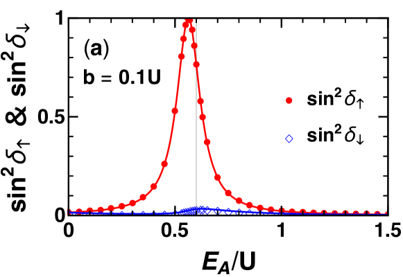
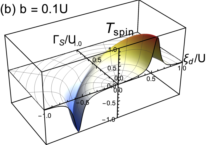
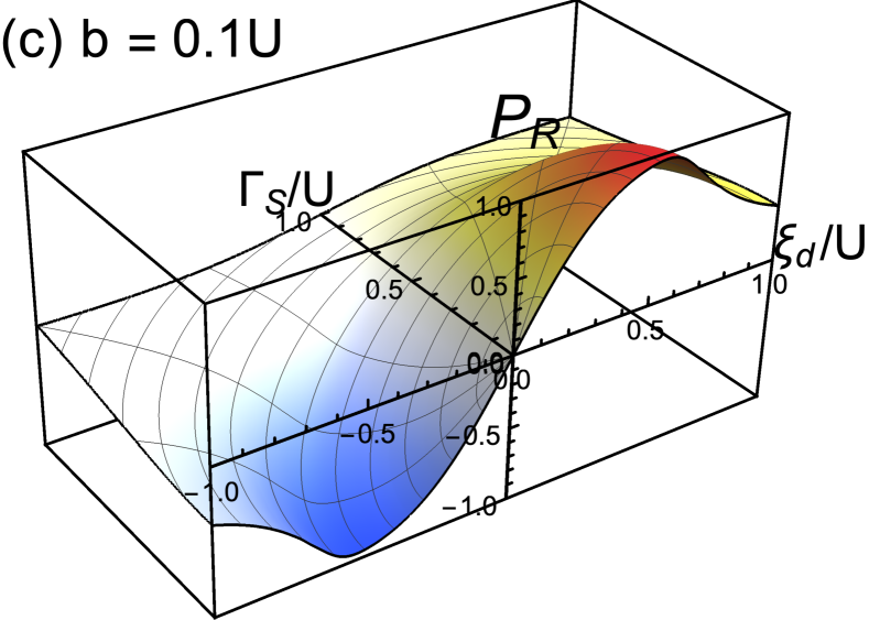
Figure 12: Spin-dependent transport coefficients at finite magnetic field $b=0.1U$, for $U/(\pi\Gamma_{N})=5.0$. Top panel (a) shows $\sin^{2}\delta_{\uparrow}$ and $\sin^{2}\delta_{\downarrow}$, plotted vs $E_{A}$. Three-dimensional figures represent (b) spin transmission coefficient $\mathcal{T}_{\mathrm{spin}}$ and (c) current polarization $P_{R}$, plotted as functions of $\xi_{d}$ and $\Gamma_{S}$, for $\Gamma_{L}=\Gamma_{R}$.

VI Summary

We have studied the interplay between the crossed Andreev reflection, Kondo effect, and Zeeman splitting, occurring in a multi-terminal quantum dot, consisting of two normal and one SC leads.

It has been shown that the linear-response currents flowing through quantum dot at zero temperature $T=0$ are determined by two angular variables, i.e., the phase shift $\delta_{\sigma}$ of Bogoliubov particles and the Bogoliubov rotation angle $\Theta=\cot^{-1}(\xi_{d}/\Gamma_{S})$ in the the limit of large SC gap $|\Delta_{S}|\to\infty$. In this limit, the phase shift can be deduced from an effective Anderson model for interacting Bogoliubov particles, which has a global U(1) symmetry along the principal axis in the Nambu pseudo-spin space. The Bogoliubov angle $\Theta$ enters the transport coefficients through the SC coherence factors, and plays an essential role in the conductance, together with the position of the Andreev level $E_{A}=\sqrt{\xi_{d}^{2}+\Gamma_{S}^{2}}$.

In the first half of the paper, we have described the role of the many-body optical theorem on the CAR, and have shown that the multi-terminal conductance at finite magnetic fields is determined by the transmission probability $\mathcal{T}_{\mathrm{BG}}=\frac{1}{2}\sum_{\sigma}\sin^{2}\delta_{\sigma}$ of the Bogoliubov particles, which does not depend on $\Theta$, and by the Cooper-pair tunneling part $\mathcal{T}_{\mathrm{CP}}=\frac{1}{4}\sin^{2}(\delta_{\uparrow}+\delta_{\downarrow})\sin^{2}\Theta$. In the second half, we have discussed the behaviors of nonlocal conductance, obtained by using the NRG approach in a wide range of the parameter space which consists of $\xi_{d}$, $\Gamma_{S}$, $\Gamma_{N}$, the Coulomb interaction $U$, and the magnetic field $b$.

At zero magnetic field, the nonlocal conductance $g_{\mathrm{RL}}$ becomes negative at $E_{A}\gtrsim U/2$ and $\pi/4<\Theta<3\pi/4$, where the CAR dominates. In particular, the contribution of Cooper-pair tunnelings $\mathcal{T}_{\mathrm{CP}}$ is maximized at a crescent-shaped crossover region between the Kondo-dominated and the SC-dominated regimes, emerging at $E_{A}\simeq U/2$ in the angular direction of $\Theta\simeq\pi/2$. The width of the crescent region along the $\Gamma_{S}$-axis is of the order of $\Gamma_{N}$. The enhanced CAR occurring in this region is caused by the valence fluctuation of the Bogoliubov particles, in the middle of which the occupation number takes the value $Q=1/2$ and the phase shift due to the Cooper-pair tunneling reaches the unitary limit $\delta_{\uparrow}+\delta_{\downarrow}=\pi/2$.

Magnetic fields lift the spin degeneracy of the Andreev resonance level. In the strongly-correlated case where $Q\simeq 1.0$ with $E_{A}\lesssim U/2$ and $U\gg\Gamma_{N}$, the crossover between the Kondo regime and Zeeman-dominated regime occurs at a magnetic field $b\sim T^{*}$ of the order of the Kondo energy scale $T^{*}$. In contrast, at $E_{A}\gtrsim U/2$ in the valence-fluctuation region of the Bogoliubov particles, magnetic fields induce a crossover between the SC-proximity dominated regime and the Zeeman-dominated regime at $b\simeq E_{A}-U/2$, where the renormalized Andreev level $\widetilde{E}_{A,\uparrow}$ for the majority spin component ($\sigma=\uparrow$) crosses the Fermi level. It induces the resonant tunneling of the Bogoliubov particles and the Cooper-pair tunneling, the transmission probabilities of which are determined by the phase shifts $\delta_{\uparrow}\simeq\pi/2$ and $\delta_{\uparrow}+\delta_{\downarrow}\simeq\pi/2$, respectively. Note that $\delta_{\downarrow}\simeq 0.0$ as the renormalized Andreev level for the minority-spin component becomes almost empty $Q_{\downarrow}\simeq 0.0$ in this region. It has also been demonstrated that the resonant spin current is enhanced in the angular direction of $\Theta\simeq 0$ or $\Theta\simeq\pi$ when the Andreev level of the majority spin crosses the Fermi level.

The nonlocal conductance $g_{\mathrm{RL}}$ becomes negative in the parameter region of $E_{A}\gtrsim U/2+b$ and $\pi/4<\Theta<3\pi/4$. In particular, the CAR contribution is maximized in the crescent-shaped region, which moves in the $\xi_{d}$ vs $\Gamma_{S}$ plane, together with the semi-circular boundary of radius $E_{A}\simeq U/2+b$ as $b$ increases. The crescent region evolves with the magnetic field and yields a flat valley structure which emerges in the $b$ dependence of $g_{\mathrm{RL}}$, at $0\leq b\lesssim E_{A}-U/2$. These results suggest that, in order to experimentally probe the CAR contributions measuring the nonlocal conductance, the crescent parameter region will be a plausible target to be examined.

Appendix A Effective Hamiltonian for $|\Delta_{S}|\to\infty$

The Hamiltonian $H$ defined in Eq. (1) can be separated into two independent parts since only the symmetrized linear combination $\alpha_{\varepsilon,\sigma}$ of conduction electrons has a finite tunnel coupling to the QD, whereas the anti-symmetrized linear combination $\beta_{\varepsilon,\sigma}$ is decoupled from the rest of the system:

$$\alpha_{\varepsilon,\sigma}\,\equiv \ \frac{v_{L}\,c_{\varepsilon,L,\sigma}+v_{R}\,c_{\varepsilon,R,\sigma}}{\sqrt{v_{L}^{2}+v_{R}^{2}}}\,,$$ (46)

$$\beta_{\varepsilon,\sigma}\,\equiv \ \frac{-v_{R}\,c_{\varepsilon,L,\sigma}+v_{L}\,c_{\varepsilon,R,\sigma}}{\sqrt{v_{L}^{2}+v_{R}^{2}}}\,.$$ (47)

Correspondingly, the conduction-electron part and the normal-tunneling part of the Hamiltonian can be rewritten in the form

$$H_{\text{N}}\,= \ \sum_{\sigma}\int_{-D}^{D}\!d\varepsilon\,\varepsilon\,\Bigl{(}\alpha^{\dagger}_{\varepsilon,\sigma}\alpha_{\varepsilon,\sigma}+\beta^{\dagger}_{\varepsilon,\sigma}\beta_{\varepsilon,\sigma}\Bigr{)},$$ (48)

$$H_{\text{TN}}= \ v_{N}\sum_{\sigma}\int_{-D}^{D}\!d\varepsilon\,\sqrt{\rho_{c}}\,\Bigl{(}\alpha^{\dagger}_{\varepsilon,\sigma}d_{\sigma}+\mathrm{H.c.}\Bigr{)}\,,$$ (49)

where $v_{N}\equiv\sqrt{v_{L}^{2}+v_{R}^{2}}$.

Furthermore, in the large gap limit $\left|\Delta_{S}\right|\to\infty$ which is taken at $\left|\Delta_{S}\right|\ll D_{S}$ keeping $\rho_{S}$ constant, the superconducting proximity effects can be described by the pair potential $\Delta_{d}\equiv\Gamma_{S}\,e^{i\phi_{S}}$ penetrating into the QD. Tanaka et al. (2007b, a) Therefore, at low energies, the subspace to which the QD belongs can be described by the following effective Hamiltonian:

$$H_{\mathrm{eff}}\,\equiv \ \ \bm{\psi}_{d}^{\dagger}\ \bm{\mathcal{H}}_{\mathrm{dot}}^{\mathrm{SC}}\ \bm{\psi}_{d}\,+\,\frac{U}{2}\left(n_{d}-1\right)^{2}$$

$$+v_{N}\int_{-D}^{D}\!\!d\varepsilon\,\sqrt{\rho_{c}}\left[\,\bm{\psi}_{\alpha}^{\dagger}(\varepsilon)\,\bm{\psi}_{d}+\bm{\psi}_{d}^{\dagger}\,\bm{\psi}_{\alpha}(\varepsilon)\,\right]$$

$$+\int_{-D}^{D}\!\!d\varepsilon\,\varepsilon\ \bm{\psi}_{\alpha}^{\dagger}(\varepsilon)\,\bm{\psi}_{\alpha}(\varepsilon)\,.$$ (50)

Here, $\bm{\mathcal{H}}_{\mathrm{dot}}^{\mathrm{SC}}$ is the following matrix defined in the Nambu pseudo-spin space,

$$\bm{\mathcal{H}}_{\mathrm{dot}}^{\mathrm{SC}}\,\equiv \ \begin{pmatrix}\xi_{d}&\Delta_{d}\cr\Delta_{d}^{*}&-\xi_{d}\rule{0.0pt}{9.95863pt}\end{pmatrix}\,-\,b\,\bm{1}\,,$$ (51)

with $\bm{1}$ the $2\times 2$ unit matrix, and

$$\bm{\psi}_{d}\equiv \ \begin{pmatrix}d_{\uparrow}\cr d_{\downarrow}^{\dagger}\rule{0.0pt}{14.22636pt}\cr\end{pmatrix},\qquad\bm{\psi}_{\alpha}(\varepsilon)\equiv\begin{pmatrix}\alpha_{\varepsilon,\uparrow}\cr-\alpha_{-\varepsilon,\downarrow}^{\dagger}\rule{0.0pt}{14.22636pt}\cr\end{pmatrix}.\rule{0.0pt}{22.76228pt}$$ (52)

The effective Hamiltonian $H_{\mathrm{eff}}$ has a global U$(1)$ symmetry with respect to the principal axis along the three-dimensional vector $\widehat{\bm{n}}\propto(\mathrm{Re}\,\Delta_{d},\,-\mathrm{Im}\,\Delta_{d},\,\xi_{d})$ in the Nambu space. The conserved charge associated with this U$(1)$ symmetry corresponds to the total number of Bogoliubov particles, the operators for which are given by

$$\begin{pmatrix}\gamma_{d,\uparrow}^{\phantom{\dagger}}\cr\gamma_{d,\downarrow}^{\dagger}\rule{0.0pt}{17.07182pt}\cr\end{pmatrix}= \ \bm{\mathcal{U}}^{\dagger}\bm{\psi}_{d},\quad\begin{pmatrix}\gamma_{\varepsilon,\uparrow}^{\phantom{\dagger}}\cr-\gamma_{-\varepsilon,\downarrow}^{\dagger}\rule{0.0pt}{17.07182pt}\cr\end{pmatrix}=\,\bm{\mathcal{U}}^{\dagger}\bm{\psi}_{\alpha}(\varepsilon)\,.$$ (53)

Here, $\bm{\mathcal{U}}$ is the unitary matrix which diagonalizes $\bm{\mathcal{H}}_{\mathrm{dot}}^{\mathrm{SC}}$:

$$\!\!\bm{\mathcal{U}}^{\dagger}\,\bm{\mathcal{H}}_{\mathrm{dot}}^{\mathrm{SC}}\ \bm{\mathcal{U}}\,=\,E_{A}\bm{\tau}_{3}-b\bm{1},\qquad\bm{\tau}_{3}=\begin{pmatrix}1&\ 0\cr 0&-1\rule{0.0pt}{5.69046pt}\end{pmatrix},$$ (54)

with $E_{A}\equiv\sqrt{\xi_{d}^{2}+\Gamma_{S}^{2}}$. For example, in the case where the Josephson phase $\phi_{S}=0$, the matrix $\bm{\mathcal{U}}$ is determined by a single Bogoliubov angle $\Theta$, as shown in Eq. (13).

Appendix B Derivation of linear nonlocal current

In this appendix, we provide a brief derivation of the nonlocal conductance defined in Eqs. (24)–(27)

The current flowing from the quantum dot to the normal lead on the right is described by the operator,

$$\widehat{I}_{R,\sigma}\,=\,-i\,ev_{R}\int_{-D}^{D}\!\!d\varepsilon\,\sqrt{\rho_{c}}\,\Bigl{(}c^{\dagger}_{\varepsilon,R,\sigma}d_{\sigma}-d^{\dagger}_{\sigma}c_{\varepsilon,R,\sigma}\Bigr{)}$$ (55)

for spin $\sigma$ component. The steady-state average of the total current $I_{R}\equiv\langle\widehat{I}_{R,\uparrow}\rangle+\langle\widehat{I}_{R,\downarrow}\rangle$ with $I_{R,\sigma}\equiv\langle\widehat{I}_{R,\sigma}\rangle$ can be expressed in terms of the Green function in the Keldysh formalism, Tanaka et al. (2007a)

$$I_{R}\,= \ -i\,\frac{e}{h}\int_{-\infty}^{\infty}\!d\omega\,\Gamma_{R}\,\mathrm{Tr}\,\Bigl{[}\bm{G}_{dd}^{r}(\omega)\,\bm{\mathcal{C}}_{R}(\omega)\,\bm{G}_{dd}^{a}(\omega)\,\bm{\tau}_{3}\Bigr{]}\,,$$

$$\bm{\mathcal{C}}_{R}\,\equiv \ \,\bm{\Sigma}_{\mathrm{tot}}^{\mathrm{K}}-\bigl{(}1-2\bm{f}_{R}\bigr{)}\Bigr{[}\,\bm{\Sigma}_{\mathrm{tot}}^{-+}-\bm{\Sigma}_{\mathrm{tot}}^{+-}\,\Bigr{]}\,.$$ (56)

Here, $\mathrm{Tr}$ denotes the trace of the $2\times 2$ matrices in the Nambu pseudo-spin space. $\bm{\Sigma}^{-+}_{\mathrm{tot}}$ and $\bm{\Sigma}^{+-}_{\mathrm{tot}}$ are the lesser and greater self-energies, respectively, and $\bm{\Sigma}^{\mathrm{K}}_{\mathrm{tot}}\equiv-\bm{\Sigma}^{-+}_{\mathrm{tot}}-\bm{\Sigma}^{+-}_{\mathrm{tot}}$. The matrix $\bm{f}_{\nu}$ is defined as

$$\bm{f}_{\nu}(\omega)=\left[\,\begin{matrix}f_{\nu}(\omega)&\ 0\cr 0\rule{0.0pt}{14.22636pt}&\ \overline{f}_{\nu}(\omega)\cr\end{matrix}\,\right],\qquad\quad\nu=L,\,R.$$ (57)

The bias voltage $eV_{\nu}$ is applied to the leads such that $f_{\nu}(\omega)\equiv f(\omega-eV_{\nu})$ and $\overline{f}_{\nu}(\omega)\equiv f(\omega+eV_{\nu})$ with $f(\omega)=1/[e^{\omega/T}+1]$ the Fermi distribution function.

Each self-energy matrix can be separated into two parts, e.g.,

$$\bm{\Sigma}^{\mathrm{K}}_{\mathrm{tot}}(\omega)\,=\,\bm{\Sigma}^{\mathrm{K}}_{0}(\omega)+\bm{\Sigma}^{\mathrm{K}}_{U}(\omega)\;.$$ (58)

Here, the first term on the right-hand side represents the tunnel contributions at $U=0$,

$$\!\!\!\!\bm{\Sigma}^{\mathrm{K}}_{0}(\omega)=-2i\sum_{\nu=L,R}\Gamma_{\nu}\Bigl{[}\,\bm{1}-2\bm{f}_{j}(\omega)\,\Bigr{]},$$ (59)

$$\!\!\!\!\bm{\Sigma}_{0}^{-+}(\omega)-\bm{\Sigma}_{0}^{+-}(\omega)\,=\,-2i\bigl{(}\Gamma_{L}+\Gamma_{R}\bigr{)}\,\bm{1}\,,$$ (60)

with $\bm{1}$ the $2\times 2$ unit matrix in the pseudo-spin space. The second term on the right-hand side of Eq. (58), $\bm{\Sigma}^{\mathrm{K}}_{U}(\omega)$, represents the self-energy corrections due to the Coulomb interaction $U$. This and the corresponding terms of the lesser and greater self-energies, $\bm{\Sigma}^{-+}_{U}(\omega)$ and $\bm{\Sigma}^{+-}_{U}(\omega)$ are also pure imaginary in the frequency domain, and represent the damping of quasiparticles due to the multiple collisions. These imaginary parts of the interacting self-energies vanish at $T=0$, $eV_{\nu}=0$, and $\omega=0$, and thus they do not contribute to the linear-response current at zero temperature. Furthermore, the function $\bm{\mathcal{C}}_{R}(\omega)$ identically vanishes at $eV_{\nu}=0$ since there is no steady current at equilibrium.

Therefore, at $T=0$, the linear-response current can be calculated, keeping the noninteracting terms in Eqs. (59) and (60) for $\bm{\mathcal{C}}_{R}(\omega)$ in the right-hand side of Eq.  (56):

$$I_{R}=\,\frac{4e^{2}}{h} \Biggl{[}\,\left(\Bigl{|}\bigl{\{}\bm{G}_{dd}^{r}(0)\bigl{\}}_{11}\Bigr{|}^{2}+\Bigl{|}\bigl{\{}\bm{G}_{dd}^{r}(0)\bigl{\}}_{22}\Bigr{|}^{2}\right)$$

$$\qquad\times\Gamma_{R}\Gamma_{L}\,(V_{L}-V_{R})$$

$$-\left(\Bigl{|}\bigl{\{}\bm{G}_{dd}^{r}(0)\bigl{\}}_{12}\Bigr{|}^{2}+\Bigl{|}\bigl{\{}\bm{G}_{dd}^{r}(0)\bigl{\}}_{21}\Bigr{|}^{2}\right)$$

$$\qquad\times\Bigl{\{}\Gamma_{R}\Gamma_{L}\,(V_{L}+V_{R})+2\Gamma_{R}^{2}\,V_{R}\Bigr{\}}\,\,\Biggr{]}.$$ (61)

Note that the anomalous Green’s functions are related to each other through $\bigl{\{}\bm{G}_{dd}^{r}(\omega)\bigl{\}}_{21}=\bigl{\{}\bm{G}_{dd}^{a}(\omega)\bigl{\}}_{12}^{*}$. Equation (61) can be rewritten further in terms of the phase shifts $\delta_{\sigma}$ and the Bogoliubov angle $\Theta$, by using Eq. (12) to obtain Eqs. (26) and (27).

Appendix C Optical theorem for Andreev scattering

We provide a derivation of the optical theorem, which emerges in the form

$$\sum_{\sigma}\sin^{2}\delta_{\sigma}\,=\,2\bigl{(}\mathcal{T}_{\mathrm{ET}}+\mathcal{T}_{\mathrm{CP}}\bigr{)}\,.$$ (62)

We start with the matrix identity for the impurity Green’s function in the Nambu form

$$\bm{G}_{dd}^{r}(\omega)-\bm{G}_{dd}^{a}(\omega)$$

$$\quad=\bm{G}_{dd}^{r}(\omega)\Bigl{[}\left\{\bm{G}_{dd}^{a}(\omega)\right\}^{-1}-\left\{\bm{G}_{dd}^{r}(\omega)\right\}^{-1}\Bigr{]}\bm{G}_{dd}^{a}(\omega)$$

$$\quad=\bm{G}_{dd}^{r}(\omega)\Bigl{[}\bm{\Sigma}_{\mathrm{tot}}^{r}(\omega)-\bm{\Sigma}_{\mathrm{tot}}^{a}(\omega)\Bigr{]}\bm{G}_{dd}^{a}(\omega)\,.$$ (63)

At $\omega=T=eV=0$, it can be rewritten further in the form

$$-\frac{\Gamma_{N}}{2i}\Bigl{[}\,\bm{G}_{dd}^{r}(0)-\bm{G}_{dd}^{a}(0)\,\Bigr{]}\,= \ \Gamma_{N}^{2}\,\bm{G}_{dd}^{r}(0)\,\bm{G}_{dd}^{a}(0)\,.$$ (64)

Here, we have used the property that the imaginary part of the interacting self-energy vanishes $\mathrm{Im}\,\bm{\Sigma}_{U}^{r}(0)=0$ and the noninteracting one is given by $\bm{\Sigma}_{0}^{r}(\omega)-\bm{\Sigma}_{0}^{a}(\omega)=-2i\Gamma_{N}\bm{1}$. Taking trace of the Nambu matrices, the left-hand side of Eq. (64) can be calculated as

$$\!\!\!\!-\frac{\Gamma_{N}}{2i}\mathrm{Tr}\,\Bigl{[}\,\bm{G}_{dd}^{r}(0)-\bm{G}_{dd}^{a}(0)\,\Bigr{]}$$

$$=-\frac{\Gamma_{N}}{2i}\sum_{\sigma}\Bigl{[}G_{\gamma,\sigma}^{r}(0)-G_{\gamma,\sigma}^{a}(0)\Bigr{]}=\sum_{\sigma}\sin^{2}\delta_{\sigma}.$$ (65)

Similarly, the right-hand side of Eq. (64) takes the form

$$\Gamma_{N}^{2}\mathrm{Tr}\,\Bigl{[}\,\bm{G}_{dd}^{r}(0)\,\bm{G}_{dd}^{r}(0)\,\Bigr{]}$$

$$=\ \Gamma_{N}^{2}\biggl{[}\Bigl{|}\left\{\bm{G}_{dd}^{r}(0)\right\}_{11}\Bigr{|}^{2}+\Bigl{|}\left\{\bm{G}_{dd}^{r}(0)\right\}_{12}\Bigr{|}^{2}$$

$$\qquad\quad+\Bigl{|}\left\{\bm{G}_{dd}^{r}(0)\right\}_{21}\Bigr{|}^{2}+\Bigl{|}\left\{\bm{G}_{dd}^{r}(0)\right\}_{22}\Bigr{|}^{2}\,\biggr{]}.$$ (66)

The last line corresponds to $2\bigl{(}\mathcal{T}_{\mathrm{ET}}+\mathcal{T}_{\mathrm{CP}}\bigr{)}$ defined in Eqs. (26) and (27), and from this Eq. (62) follows.

Appendix D Derivation of the spin-current formula

We briefly describe here the linear-response formula for the spin current following between two normal leads at finite magnetic fields. The current formula presented in Appendix B can be decomposed into the contributions of the $\uparrow$- and $\downarrow$- spin components, which can be rearranged as a spin current:

$$I_{R,\mathrm{spin}}\equiv I_{R,\uparrow}-I_{R,\downarrow}$$

$$=\ -i\,\frac{e}{h}\int_{-\infty}^{\infty}\!d\omega\,\Gamma_{R}\,\mathrm{Tr}\Bigl{[}\bm{G}_{dd}^{r}(\omega)\,\bm{\mathcal{C}}_{R}(\omega)\,\bm{G}_{dd}^{a}(\omega)\,\Bigr{]}\,.$$ (67)

Specifically at $T=0$, the linear-response spin current can be expressed in the following form,

$$I_{R,\mathrm{spin}}\,= \ \frac{4e^{2}}{h}\,\Gamma_{L}\Gamma_{R}\left(\Bigl{|}\bigl{\{}\bm{G}_{dd}^{r}(0)\bigl{\}}_{11}\Bigr{|}^{2}-\Bigl{|}\bigl{\{}\bm{G}_{dd}^{r}(0)\bigl{\}}_{22}\Bigr{|}^{2}\right)$$

$$\times\left(V_{L}-V_{R}\right)$$

$$= \ \frac{4e^{2}}{h}\,\frac{\Gamma_{L}\Gamma_{R}}{\Gamma_{N}^{2}}\,\mathcal{T}_{\mathrm{spin}}\,\left(V_{L}-V_{R}\right)\,,$$ (68)

$$\mathcal{T}_{\mathrm{spin}}\,\equiv \ \left(\sin^{2}\delta_{\uparrow}-\sin^{2}\delta_{\downarrow}\right)\cos\Theta\,.$$ (69)

Note that $I_{L,\uparrow}-I_{L,\downarrow}=I_{R,\uparrow}-I_{R,\downarrow}$.

Similarly, the current polarization $P_{R}$, defined with respect to symmetric voltages $V_{L}=-V_{R}$, can be used as a measure of the spin current relative to the charge current López and Sánchez (2003); Souza et al. (2008); Hitachi et al. (2006); Kiyama et al. (2015):

$$P_{R}\,\equiv\,\frac{I_{R,\uparrow}-I_{R,\downarrow}}{I_{R,\uparrow}+I_{R,\downarrow}}\ =\ \frac{\Gamma_{L}\Gamma_{R}\mathcal{T}_{\mathrm{spin}}}{2\left[\Gamma_{L}\Gamma_{R}\mathcal{T}_{\mathrm{ET}}+\Gamma_{R}^{2}\mathcal{T}_{\mathrm{CP}}\right]}$$

$$\ \ \xrightarrow{\,\Gamma_{L}=\Gamma_{R}\,}\ \frac{\sin^{2}\delta_{\uparrow}-\sin^{2}\delta_{\downarrow}}{\sin^{2}\delta_{\uparrow}+\sin^{2}\delta_{\downarrow}}\,\cos\Theta\,.$$ (70)

References

- Hofstetter et al. (2009) L. Hofstetter, S. Csonka, J. Nygård, and C. Schönenberger, Nature 461, 960 (2009).
- Schindele et al. (2012) J. Schindele, A. Baumgartner, and C. Schönenberger, Phys. Rev. Lett. 109, 157002 (2012).
- Das et al. (2012) A. Das, Y. Ronen, M. Heiblum, D. Mahalu, A. V. Kretinin, and H. Shtrikman, Nature Communications 3, 1165 (2012).
- Schindele et al. (2014) J. Schindele, A. Baumgartner, R. Maurand, M. Weiss, and C. Schönenberger, Phys. Rev. B 89, 045422 (2014).
- Fülöp et al. (2014) G. Fülöp, S. d’Hollosy, A. Baumgartner, P. Makk, V. A. Guzenko, M. H. Madsen, J. Nygård, C. Schönenberger, and S. Csonka, Phys. Rev. B 90, 235412 (2014).
- Tan et al. (2015) Z. B. Tan, D. Cox, T. Nieminen, P. Lähteenmäki, D. Golubev, G. B. Lesovik, and P. J. Hakonen, Phys. Rev. Lett. 114, 096602 (2015).
- Borzenets et al. (2016) I. V. Borzenets, Y. Shimazaki, G. F. Jones, M. F. Craciun, S. Russo, M. Yamamoto, and S. Tarucha, Scientific Reports 6, 23051 (2016).
- Tan et al. (2021) Z. B. Tan, A. Laitinen, N. S. Kirsanov, A. Galda, V. M. Vinokur, M. Haque, A. Savin, D. S. Golubev, G. B. Lesovik, and P. J. Hakonen, Nature Communications 12, 138 (2021).
- Golubev and Zaikin (2007) D. S. Golubev and A. D. Zaikin, Phys. Rev. B 76, 184510 (2007).
- Eldridge et al. (2010) J. Eldridge, M. G. Pala, M. Governale, and J. König, Phys. Rev. B 82, 184507 (2010).
- Sánchez et al. (2018) R. Sánchez, P. Burset, and A. L. Yeyati, Phys. Rev. B 98, 241414 (2018).
- Wrześniewski and Weymann (2017) K. Wrześniewski and I. Weymann, Phys. Rev. B 96, 195409 (2017).
- Rech et al. (2012) J. Rech, D. Chevallier, T. Jonckheere, and T. Martin, Phys. Rev. B 85, 035419 (2012).
- Walldorf et al. (2018) N. Walldorf, C. Padurariu, A.-P. Jauho, and C. Flindt, Phys. Rev. Lett. 120, 087701 (2018).
- Hussein et al. (2019) R. Hussein, M. Governale, S. Kohler, W. Belzig, F. Giazotto, and A. Braggio, Phys. Rev. B 99, 075429 (2019).
- Wójcik and Weymann (2019) K. P. Wójcik and I. Weymann, Phys. Rev. B 99, 045120 (2019).
- Walldorf et al. (2020) N. Walldorf, F. Brange, C. Padurariu, and C. Flindt, Phys. Rev. B 101, 205422 (2020).
- Lee et al. (2014) E. J. H. Lee, X. Jiang, M. Houzet, R. Aguado, C. M. Lieber, and S. De Franceschi, Nature Nanotechnology 9, 79 (2014).
- Bordoloi et al. (2022) A. Bordoloi, V. Zannier, L. Sorba, C. Schönenberger, and A. Baumgartner, Nature 612, 454 (2022).
- Choi et al. (2000) M.-S. Choi, C. Bruder, and D. Loss, Phys. Rev. B 62, 13569 (2000).
- Wang and Hu (2011) Z. Wang and X. Hu, Phys. Rev. Lett. 106, 037002 (2011).
- Deacon et al. (2015) R. S. Deacon, A. Oiwa, J. Sailer, S. Baba, Y. Kanai, K. Shibata, K. Hirakawa, and S. Tarucha, Nature Communications 6, 7446 (2015).
- Padurariu et al. (2017) C. Padurariu, T. Jonckheere, J. Rech, T. Martin, and D. Feinberg, Phys. Rev. B 95, 205437 (2017).
- Yokoyama and Nazarov (2015) T. Yokoyama and Y. V. Nazarov, Phys. Rev. B 92, 155437 (2015).
- Ueda et al. (2019) K. Ueda, S. Matsuo, H. Kamata, S. Baba, Y. Sato, Y. Takeshige, K. Li, S. Jeppesen, L. Samuelson, H. Xu, and S. Tarucha, Science Advances 5, eaaw2194 (2019).
- Cadden-Zimansky and Chandrasekhar (2006) P. Cadden-Zimansky and V. Chandrasekhar, Phys. Rev. Lett. 97, 237003 (2006).
- Lesovik, G. B. et al. (2001) Lesovik, G. B., Martin, T., and Blatter, G., Eur. Phys. J. B 24, 287 (2001).
- Russo et al. (2005) S. Russo, M. Kroug, T. M. Klapwijk, and A. F. Morpurgo, Phys. Rev. Lett. 95, 027002 (2005).
- Yeyati et al. (2007) A. L. Yeyati, F. S. Bergeret, A. Martín-Rodero, and T. M. Klapwijk, Nature Physics 3, 455 (2007).
- Cadden-Zimansky et al. (2009) P. Cadden-Zimansky, J. Wei, and V. Chandrasekhar, Nature Physics 5, 393 (2009).
- Wei and Chandrasekhar (2010) J. Wei and V. Chandrasekhar, Nature Physics 6, 494 (2010).
- Golubev and Zaikin (2019) D. S. Golubev and A. D. Zaikin, Phys. Rev. B 99, 144504 (2019).
- Kirsanov et al. (2019) N. S. Kirsanov, Z. B. Tan, D. S. Golubev, P. J. Hakonen, and G. B. Lesovik, Phys. Rev. B 99, 115127 (2019).
- Ranni et al. (2021) A. Ranni, F. Brange, E. T. Mannila, C. Flindt, and V. F. Maisi, Nature Communications 12, 6358 (2021).
- Yoshioka and Ohashi (2000) T. Yoshioka and Y. Ohashi, J. Phys. Soc. Jpn. 69, 1812 (2000).
- Tanaka et al. (2007a) Y. Tanaka, N. Kawakami, and A. Oguri, J. Phys. Soc. Jpn. 76, 074701 (2007a).
- Buizert et al. (2007) C. Buizert, A. Oiwa, K. Shibata, K. Hirakawa, and S. Tarucha, Phys. Rev. Lett. 99, 136806 (2007).
- Deacon et al. (2010a) R. S. Deacon, Y. Tanaka, A. Oiwa, R. Sakano, K. Yoshida, K. Shibata, K. Hirakawa, and S. Tarucha, Phys. Rev. Lett. 104, 076805 (2010a).
- Deacon et al. (2010b) R. S. Deacon, Y. Tanaka, A. Oiwa, R. Sakano, K. Yoshida, K. Shibata, K. Hirakawa, and S. Tarucha, Phys. Rev. B 81, 121308 (2010b).
- Yamada et al. (2011) Y. Yamada, Y. Tanaka, and N. Kawakami, Phys. Rev. B 84, 075484 (2011).
- Governale et al. (2008) M. Governale, M. G. Pala, and J. König, Phys. Rev. B 77, 134513 (2008).
- Oguri et al. (2013) A. Oguri, Y. Tanaka, and J. Bauer, Phys. Rev. B 87, 075432 (2013).
- Koga (2013) A. Koga, Phys. Rev. B 87, 115409 (2013).
- Domański et al. (2017) T. Domański, M. Žonda, V. Pokorný, G. Górski, V. Janiš, and T. Novotný, Phys. Rev. B 95, 045104 (2017).
- Vecino et al. (2003) E. Vecino, A. Martín-Rodero, and A. L. Yeyati, Phys. Rev. B 68, 035105 (2003).
- Oguri et al. (2004) A. Oguri, Y. Tanaka, and A. C. Hewson, J. Phys. Soc. Jpn. 73, 2494 (2004).
- Tanaka et al. (2007b) Y. Tanaka, A. Oguri, and A. C. Hewson, New J. Phys. 9, 115 (2007b).
- Lee et al. (2022) M. Lee, R. López, H. Q. Xu, and G. Platero, Phys. Rev. Lett. 129, 207701 (2022).
- Pillet et al. (2013) J.-D. Pillet, P. Joyez, R. Žitko, and M. F. Goffman, Phys. Rev. B 88, 045101 (2013).
- Kadlecová et al. (2017) A. Kadlecová, M. Žonda, and T. Novotný, Phys. Rev. B 95, 195114 (2017).
- Pokorný and Žonda (2023) V. Pokorný and M. Žonda, Phys. Rev. B 107, 155111 (2023).
- Filippone et al. (2018) M. Filippone, C. P. Moca, A. Weichselbaum, J. von Delft, and C. Mora, Phys. Rev. B 98, 075404 (2018).
- Oguri and Hewson (2018) A. Oguri and A. C. Hewson, Phys. Rev. B 97, 035435 (2018).
- Futterer et al. (2009) D. Futterer, M. Governale, M. G. Pala, and J. König, Phys. Rev. B 79, 054505 (2009).
- Michałek et al. (2013) G. Michałek, B. R. Bułka, T. Domański, and K. I. Wysokiński, Phys. Rev. B 88, 155425 (2013).
- Michałek et al. (2015) G. Michałek, T. Domański, B. R. Bułka, and K. I. Wysokiński, Scientific Reports 5, 14572 (2015).
- Trocha and Wrześniewski (2018) P. Trocha and K. Wrześniewski, J. Phys.: Condens. Matter 30, 305303 (2018).
- Weymann and Trocha (2014) I. Weymann and P. Trocha, Phys. Rev. B 89, 115305 (2014).
- Wójcik and Weymann (2014) K. P. Wójcik and I. Weymann, Phys. Rev. B 89, 165303 (2014).
- Weymann and Wójcik (2015) I. Weymann and K. P. Wójcik, Phys. Rev. B 92, 245307 (2015).
- Zhao and Wang (2001) H.-K. Zhao and J. Wang, Phys. Rev. B 64, 094505 (2001).
- Górski et al. (2020) Górski, K. Kucab, and T. Domański, Journal of Physics: Condensed Matter 32, 445803 (2020).
- Yamada et al. (2007) Y. Yamada, Y. Tanaka, and N. Kawakami, Phys. E (Amsterdam) 40, 265 (2007).
- Domański et al. (2008) T. Domański, A. Donabidowicz, and K. I. Wysokiński, Phys. Rev. B 78, 144515 (2008).
- Domański et al. (2016) T. Domański, I. Weymann, M. Barańska, and G. Górski, Scientific Reports 6, 23336 (2016).
- Žitko et al. (2015) R. Žitko, J. S. Lim, R. López, and R. Aguado, Phys. Rev. B 91, 045441 (2015).
- Nozières (1974) P. Nozières, J. Low Temp. Phys. 17, 31 (1974).
- Yamada (1975a) K. Yamada, Prog. Theor. Phys. 53, 970 (1975a).
- Yamada (1975b) K. Yamada, Prog. Theor. Phys. 54, 316 (1975b).
- Shiba (1975) H. Shiba, Prog. Theor. Phys. 54, 967 (1975).
- Yoshimori (1976) A. Yoshimori, Prog. Theor. Phys. 55, 67 (1976).
- Krishna-murthy et al. (1980a) H. R. Krishna-murthy, J. W. Wilkins, and K. G. Wilson, Phys. Rev. B 21, 1003 (1980a).
- Krishna-murthy et al. (1980b) H. R. Krishna-murthy, J. W. Wilkins, and K. G. Wilson, Phys. Rev. B 21, 1044 (1980b).
- Hewson et al. (2004) A. C. Hewson, A. Oguri, and D. Meyer, Eur. Phys. J. B 40, 177 (2004).
- Blanter and Büttiker (2000) Y. Blanter and M. Büttiker, Physics Reports 336, 1 (2000).
- Oguri et al. (2022) A. Oguri, Y. Teratani, K. Tsutsumi, and R. Sakano, Phys. Rev. B 105, 115409 (2022).
- López and Sánchez (2003) R. López and D. Sánchez, Phys. Rev. Lett. 90, 116602 (2003).
- Souza et al. (2008) F. M. Souza, A. P. Jauho, and J. C. Egues, Phys. Rev. B 78, 155303 (2008).
- Hitachi et al. (2006) K. Hitachi, M. Yamamoto, and S. Tarucha, Phys. Rev. B 74, 161301 (2006).
- Kiyama et al. (2015) H. Kiyama, T. Nakajima, S. Teraoka, A. Oiwa, and S. Tarucha, Phys. Rev. B 91, 155302 (2015).