Correcting force error-induced underestimation of lattice thermal conductivity in machine learning molecular dynamics
Abstract
Machine learned potentials (MLPs) have been widely employed in molecular dynamics (MD) simulations to study thermal transport. However, literature results indicate that MLPs generally underestimate the lattice thermal conductivity (LTC) of typical solids. Here, we quantitatively analyze this underestimation in the context of the neuroevolution potential (NEP), which is a representative MLP that balances efficiency and accuracy. Taking crystalline silicon, GaAs, graphene, and PbTe as examples, we reveal that the fitting errors in the machine-learned forces against the reference ones are responsible for the underestimated LTC as they constitute external perturbations to the interatomic forces. Since the force errors of a NEP model and the random forces in the Langevin thermostat both follow a Gaussian distribution, we propose an approach to correcting the LTC by intentionally introducing different levels of force noises via the Langevin thermostat and then extrapolating to the limit of zero force error. Excellent agreement with experiments is obtained by using this correction for all the prototypical materials over a wide range of temperatures. Based on spectral analyses, we find that the LTC underestimation mainly arises from increased phonon scatterings in the low-frequency region caused by the random force errors.
I Introduction
Lattice thermal conductivity (LTC) of solids is a crucial physical property in many applications including thermal management of electronics [1, 2], thermoelectric energy conversion [3, 4, 5], and thermal barrier coatings [6, 7]. Predicting and engineering LTC [8] is therefore of broad interest. Nevertheless, challenges abound owing to the presence of complex structures [9], defects [10], and disorders [10]. Among various approaches to calculating LTC [11], molecular dynamics (MD) simulation plays a unique role due to its versatility and its natural inclusion of the full lattice anharmonicity. MD simulations are widely applicable in crystals, glasses [12], and also liquids [13]. Two basic categories are commonly used, including equilibrium molecular dynamics (EMD) base on the Green-Kubo formalism [14, 15] and non-equilibrium molecular dynamics (NEMD) based on Fourier’s law of heat conduction. Notably, the homogeneous non-equilibrium molecular dynamics (HNEMD) method, initially developed by Evans [16] for pairwise interactions and recently generalized to many-body interactions [17], offers great efficiency for LTC calculations. However, the applicability and predictive power of MD simulations have long been limited by the availability and accuracy of empirical interatomic potentials.
A promising solution to this issue involves constructing machine learned potentials (MLPs) trained against reference energies, forces, and virial stresses of diverse atomic structures calculated at the quantum mechanical level. Many MLPs have been used for thermal conductivity modeling. Enabled by MLPs, the LTCs of many crystals with strong phonon anharmonicity or disorder have been successfully obtained through MD simulation driven by MLP (MLMD), including e.g., amorphous GeTe [18], SnSe [19], PbTe [20], metal-organic frameworks [21], and PH4AlBr4 [22]. Moreover, with proper quantum corrections, quantitative agreement with experimental data has also been achieved for amorphous materials [23, 24] and liquid water [25] over a wide range of temperatures. Despite these successes, previous works have also shown that for materials with relatively high LTCs, such as CoSb3 [26] and cubic silicon (c-Si) [27], the predicted LTCs from MLMD calculations are generally lower than the experimental values. To the best of our knowledge, this discrepancy remains to be systematically understood and corrected, which constitutes the main focus of our present work.
In light of the critical impact of the interatomic forces on the accuracy of MD simulations, we first evaluate the effect of random forces on LTC using HNEMD simulations with a Langevin thermostat [28] based on empirical potentials. A decrease in LTC with increasing level of random forces is consistently observed in six representative materials: amorphous silicon (a-Si), c-Si, cubic germanium (c-Ge), Si-Ge alloy, graphene, and -carbon nanotube (CNT). Subsequently, we focus on four benchmark materials including c-Si, GaAs, graphene, and PbTe, and perform LTC calculations using MLMD. In particular, we employ the neuroevolution potential (NEP) [29, 30, 31] for its balanced efficiency and accuracy. Similar to literature results, we observe a consistent underestimation of LTC from the MLMD simulations, as compared to the experimental values. However, since the residual force errors of a NEP model and the random forces (white noises) in the Langevin thermostat both follow a Gaussian distribution, we propose an approach to correcting the LTC by intentionally introducing different levels of force noises via the Langevin thermostat and then extrapolating to the limit of zero force error. This extrapolation successfully corrects the LTCs, leading to excellent agreement with experimental data for all the materials considered in a wide range of temperatures. Spectral analyses reveal that the LTC underestimation before the correction mainly originates from increased phonon scatterings at low frequencies caused by the force errors.
II Methods
II.1 Neuroevolution potential
II.1.1 The NEP formalism
In this section, we briefly review the NEP formalism [29, 30, 31]. NEP uses a feedforward neural network to correlate a local descriptor with the site energy of atom . In a single-hidden-layer neural network comprising hidden neurons, is expressed as:
| (1) |
where is the number of descriptor components, is the -th descriptor component of atom , , , , and are the trainable parameters, and is the nonlinear activation function in the hidden layer.
The descriptor vector in NEP includes radial and angular components. The radial components are defined as
| (2) |
where is the distance between atoms and and are a set of radial functions, each of which is formed by a linear combination of Chebyshev polynomials. The angular components include the so-called -body () correlations. For example, the -body ones , are defined as
| (3) |
Here, is the Legendre polynomial and is the angle formed by the and bonds. Note that the radial functions for the radial and angular descriptor components can have different cutoff radii, which are denoted as and , respectively. The free parameters are optimized using the separable natural evolutionary strategy [32] by minimizing a loss function that is a weighted sum of the root-mean-square errors (RMSEs) of energy, force, and virial stress, for generations with a population size of . The hyperparameters used for all the materials considered in this work are listed in Table S1.
II.1.2 Training datasets
For c-Si, GaAs, graphene, and PbTe, we generate datasets through density functional theory (DFT) calculations using the vasp [33] with the ion-electron interactions described by the projector-augmented wave method [33, 34]. For GaAs, the Perdew-Zunger functional with the local density approximation [35] is used to describe the exchange-correlation of electrons, while the Perdew-Burke-Ernzerhof functional with the generalized gradient approximation [36] is used for the other materials. The cutoff energy is 400 eV for PbTe and 600 eV for the other materials. The k-point mesh is for c-Si, for GaAs and PbTe, and for graphene. The energy convergence threshold is eV for c-Si and graphene and eV for GaAs and PbTe.
The dataset for each materials consists of structures from ab initio molecular dynamics (AIMD) simulations (called AIMD structures below) possibly supplemented by those from random cell deformations and atom displacements (called perturbation structures below). For c-Si, there are 900 AIMD structures sampled at various temperatures (100 K to 1000 K) and strain states (unstrained, uniaxial strains of and , biaxial strains of and ) and 70 perturbation structures. Each c-Si structure has 64 atoms. For GaAs, there are 197 AIMD structures sampled at various temperatures (100 K to 900 K) in the ensemble and 99 perturbation structures up to ±4% strains. Each GaAs structure has 250 atoms. For graphene, there are 700 AIMD structures sampled at various temperatures (100 K to 1000 K) and strain states (unstrained, biaxial strains of , , and ). Each graphene structure has 72 atoms. For PbTe, there are 60 AIMD structures sampled from 100 to 1100 K with fixed cell and 64 perturbation structures up to ±4% strains. Each PbTe structure has 216 atoms.
II.2 Thermal conductivity calculation using MD
II.2.1 The HNEMD method
We use the efficient HNEMD method [17] for many-body potentials to calculate the LTCs. In HNEMD, an external driving force on each atom
| (4) |
is applied during the simulation. Here, is the driving force parameter (of the dimension of inverse length) and [29, 31]
| (5) |
is the virial tensor of atom , where is the site energy of atom , , being the position of atom . The driving force parameter should be large enough to ensure a large signal-to-noise ratio and be small enough to maintain the system in the linear-response regime. In the linear-response regime, the LTC tensor can be calculated from the following relation [17]:
| (6) |
where represents a non-equilibrium ensemble average of the heat current, is the system temperature, and is the system volume. The heat current for the NEP model has been derived to be [29, 31]
| (7) |
where is the velocity of atom .
The HNEMD formalism also allows for an efficient calculation of the frequency-resolved LTC via the following relation [17]:
| (8) |
where
| (9) |
is the virial-velocity correlation function.
II.2.2 Thermostats in HNEMD simulations
HNEMD simulations are normally performed in the ensemble realized by using a global thermostat such as the Nosé-Hoover chain (NHC) [38] or the Bussi-Donadio-Parrinello [39] thermostat. In contrast, a local thermostat such as the Langevin thermostat [28] is avoided because it can introduce (white) noises through random forces, leading to the following equations of motion:
| (10) |
Here, is a time parameter, , , are respectively the position, momentum, and mass of atom , is the force on atom resulting from the interatomic potential, and is the random force on atom . Each component of the random force forms a Gaussian distribution with zero mean and a variance of
| (11) |
where is the average atom mass in the system, is the Boltzmann constant and is the integration time step. The random forces can affect the dynamics of the system and thus time-correlation properties such as the heat current autocorrelation function, leading to reduced LTC as compared to the case of using a global thermostat. Clearly, a smaller gives a larger random force variance and a stronger reduction of the LTC. We will demonstrate this effect using examples.
II.2.3 MD simulation details
All the MD simulations are performed using the gpumd package [37] (the gpumd executable), with a time steps of 1 fs.
For all the materials, we use a sufficiently large simulation cell to eliminate finite-size effects.
In MD simulations with empirical potentials, the simulation cells contain atoms for Si-Ge alloy, c-Ge, c-Si, and a-Si, atoms for graphene, and atoms for the -CNT. The a-Si samples are prepared by employing a melt-quench-anneal process, first equilibrating at 2000 K for 10 ns, then quenching down to 300 K during 30 ns, and finally annealing at 300 K for 10 ns. In MD simulations with NEP models, the simulation cells contain , , , and atoms for c-Si, GaAs, graphene, and PbTe, respectively. For each material, we first equilibrate the system in the ensemble (with a target pressure of zero) for 2 ns and ensemble for another 2 ns, and then calculate the LTC in the ensemble during a production time of 10 to 20 ns. For each material at each temperature, three to five independent runs are performed to improve the statistical accuracy and obtain an error estimate.
III Results and discussion
III.1 Thermal conductivity underestimation in MLMD
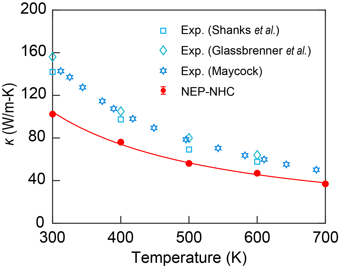
To begin with, we take c-Si as an example to demonstrate the thermal conductivity underestimation in MLMD simulations, using NEP as a representative MLP. As illustrated in Fig. 1, the calculated LTC values from 300 K to 700 K are consistently lower than experimental measurements, especially at low temperatures. For instance, at 300 K, MLMD simulations yield a LTC of W/m-K. While this is more accurate than the value of 240 W/m-K as obtained from a Stillinger-Weber potential [43], it is still approximately 32% lower than the experimental value of about 150 W/m-K [40]. An EMD simulation based on the Gaussian approximation potential also reported a lower-than-experiment value of 121 W/m-K [27]. Further, a similar trend of underestimation is observed at other temperatures for c-Si [27] and in the case of CoSb3 [26].
III.2 Role of force noises in reducing LTC
| (K) | (meV/Å) | |||
|---|---|---|---|---|
| c-Si | GaAs | graphene | PbTe | |
| 300 | 16.7 | 16.6 | 29.2 | 27.0 |
| 400 | 21.3 | 19.8 | 30.1 | 29.9 |
| 500 | 28.3 | 23.5 | 32.5 | 34.4 |
| 600 | 30.1 | 26.8 | 36.6 | 37.1 |
| 700 | 41.6 | 30.2 | 42.4 | 42.1 |
To understand the underestimation of the LTC from MLMD simulations, we notice that a MLP usually has a certain level of error for force prediction compared to the reference data. The RMSEs of force prediction for the four materials we considered at different temperatures are presented in Table 1.
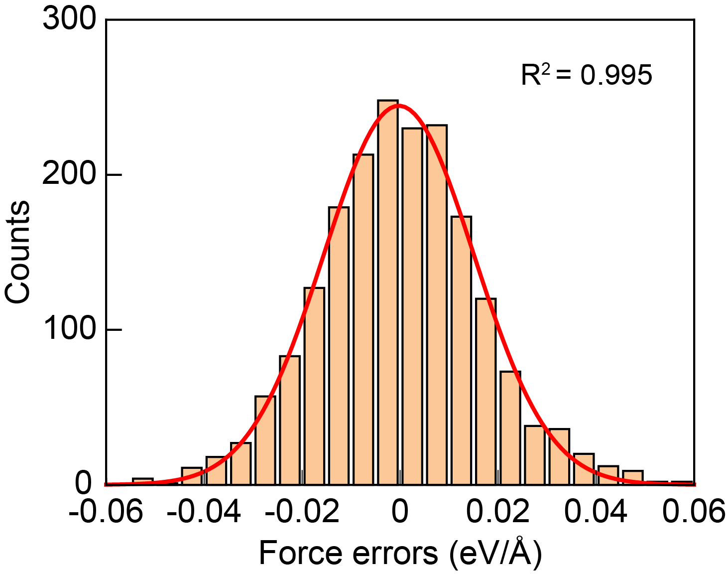
A crucial observation is that the force errors follow a Gaussian distribution, as shown in Fig. 2 for the example of c-Si at 300 K. This distribution is the same as that for the random forces in the Langevin thermostat, i.e., a Gaussian distribution with zero mean and a certain variance. Based on this similarity, an understanding of the underestimation of the LTC by MLMD simulations can thus be obtained by studying the effect of the Langevin thermostat on the LTC. One could directly use a NEP model, but due to the lower computational cost of empirical potentials, we first use the Tersoff empirical potential [44] to study this effect.
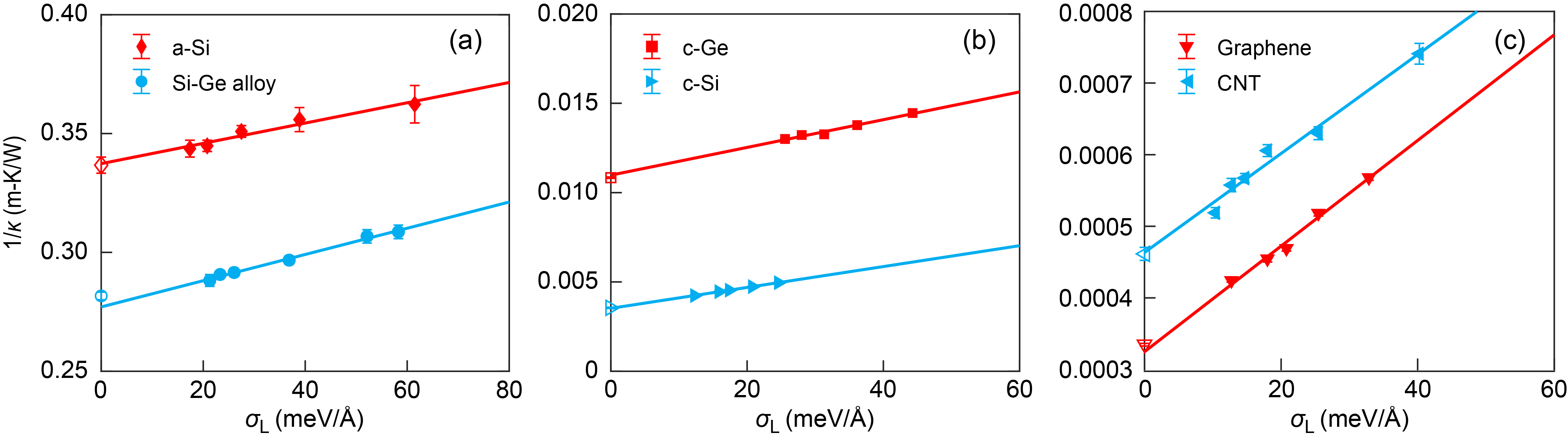
Figure 3 shows the inverse LTC () at 300 K as a function of for six representative materials, including a-Si, Si-Ge alloy, c-Ge, c-Si, graphene, and -CNT. As expected, increases with increasing , which indicates a stronger effect of the random forces in the Langevin thermostat in reducing the calculated LTC. Notably, for all the six materials, exhibits a linear relationship with . This suggests that the intrinsic LTC without the influence of the random forces in the Langevin thermostat can be obtained by extrapolating to . Indeed, the extrapolated values align well with the results from HNEMD simulations based on the NHC thermostat that does not involve random forces, with the largest relative error being (see Table S2).
The linear relation between and can be justified based on the kinetic theory of phonons and Matthiessen’s rule. Taking the random forces in the Langevin thermostat as an extra source of phonon scattering, we have
| (12) |
where and are the LTCs with and without the influence of the random forces, respectively, is the heat capacity, is the phonon group velocity, and is the phonon mean free path resulting from the random forces in the Langevin thermostat. Under first-order approximation with sufficiently small , should be proportional to , which brings Eq. 12 to
| (13) |
which gives the observed linear relation between and with being a slope parameter.
III.3 Correction of LTC in MLMD
Based on the results above, we can understand why MLMD usually underestimates the LTC, particularly for high- materials. According to the linear relation between the inverse LTC and the random force variance, we can devise a method to correct the underestimation of LTC due to the force errors in MLMD. To this end, we note that both the force errors in MLMD and the random forces in the Langevin thermostat follow a Gaussian distribution, and when they are present simultaneously, a new set of force errors are created with a larger variance given by
| (14) |
according to the properties of Gaussian distribution. Therefore, we can intentionally introduce extra force errors by using MLP-based HNEMD simulations with the Langevin thermostat. The LTC without any force errors (including the force errors of the MLP) can be obtained by an extrapolation based on the following relation:
| (15) |
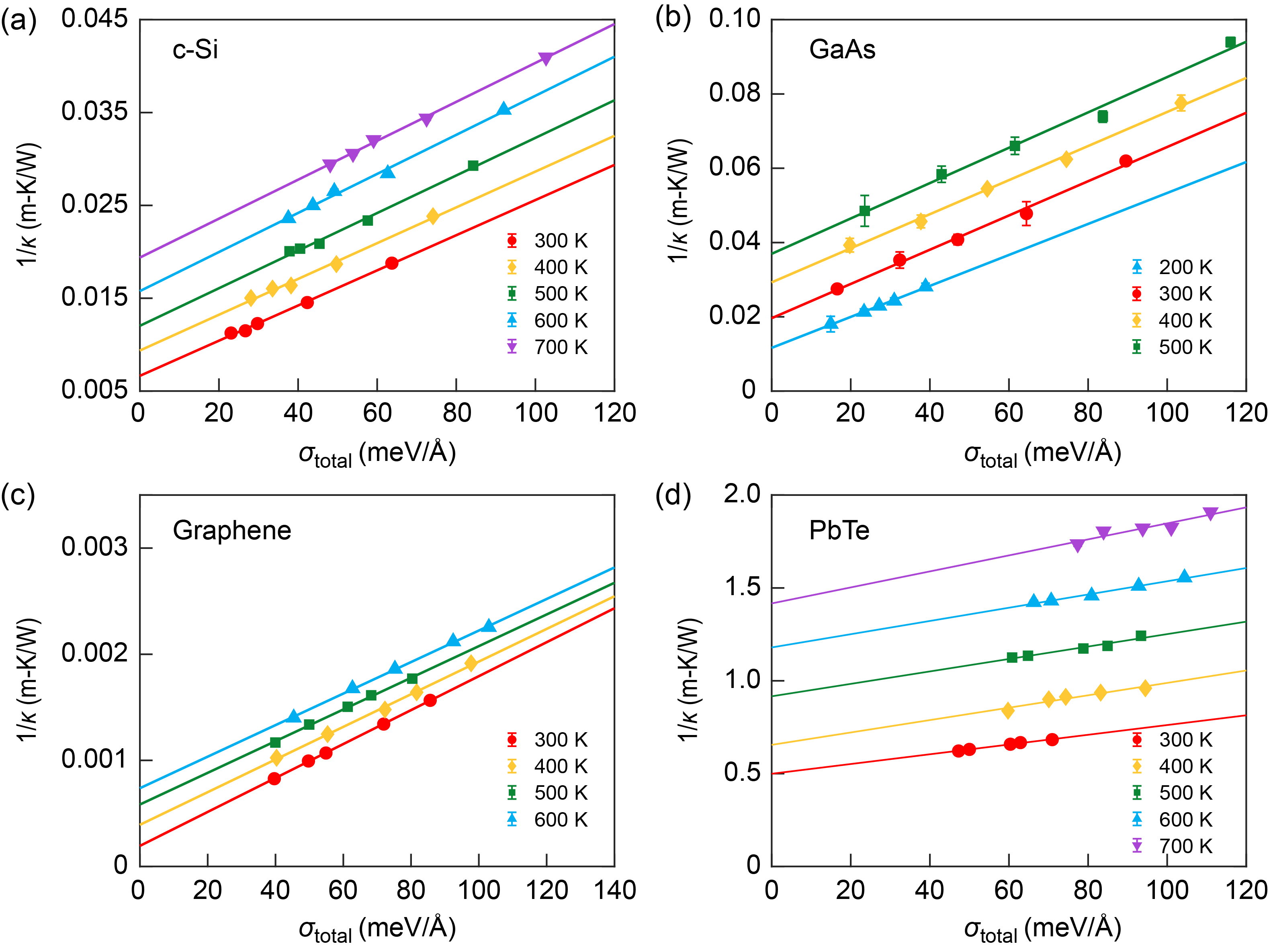
where is the LTC of a material calculated by using MLMD with a certain force error variance and the Lagevin thermostat with a certain random force variance . The linear relation between and is unfailingly confirmed in Fig. 4 for the four representative materials we considered in a wide range of temperatures, whose LTCs span three orders of magnitude.
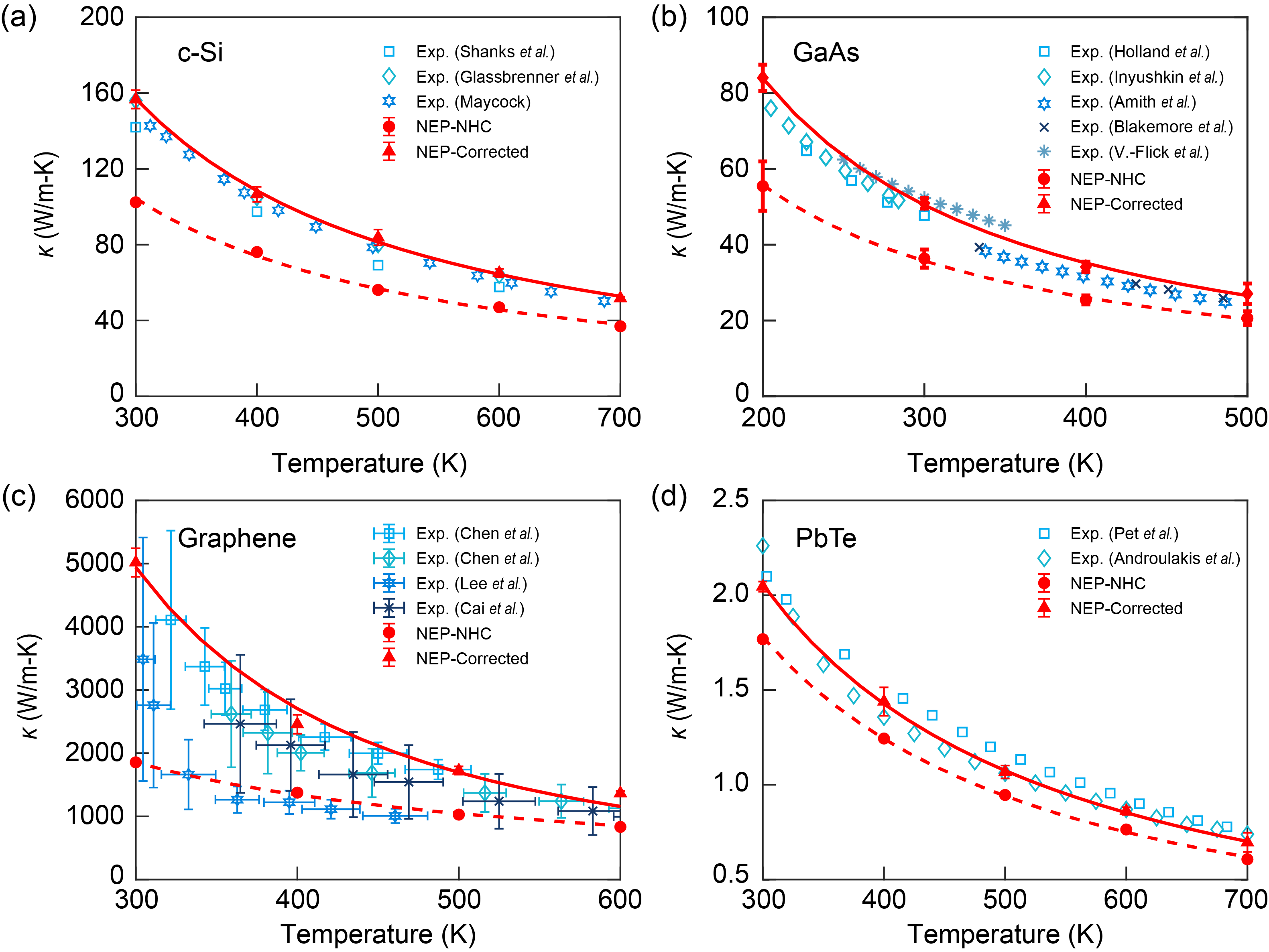
In Fig. 5, we compare the uncorrected and corrected LTCs from MLMD simulations with experimental results for c-Si, GaAs, graphene, and PbTe. In all the systems, the uncorrected LTCs are consistently lower than the experimental results in the entire temperature range due to the presence of force errors in the MLPs. Remarkably, once the force errors in the MLPs are eliminated via our extrapolation scheme, the LTCs closely approach the experimental data at all the temperatures studied. For graphene, the corrected LTCs slightly exceed the measured values but remain within the experimental uncertainties. This minor discrepancy could arise from factors such as isotope scattering and finite-size effects in the experimental setups [50, 51, 52, 53], which generally lead to reduced LTCs.
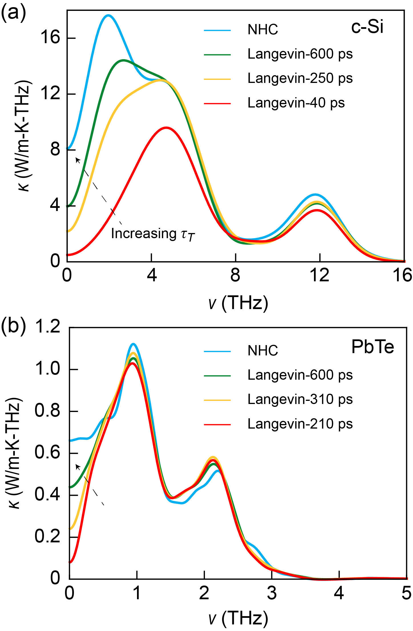
The need for LTC correction is more pronounced in materials with higher LTCs and at lower temperatures, highlighting the more significant impact of force errors when anharmonic phonon scattering is weak. This explains why the amount of correction is large for graphene that is one of the most thermally conductive material, intermediate for c-Si and GaAs that have intermediate LTCs, and small for PbTe that has low LTC. Furthermore, the spectral LTC results in Fig. 6 show that the force errors mainly reduce in the low-frequency region. With increasing force errors, in the low-frequency region is more and more reduced. This further supports the large effect of the force errors in high-LTC materials, which usually have large in the low-frequency region. Therefore, MLMD simulations remain largely accurate for low-LTC materials, such as PbTe [20], a-Si [23], amorphous SiO2 [24], and liquid water [25].
IV Conclusions
In summary, our systematic investigation revealed that the underestimation of lattice thermal conductivity commonly observed in the literature are primarily due to force fitting errors in machine learned potentials. Using empirical potentials and Langevin thermostat we demonstrated that introducing random forces on atoms can significantly reduce the lattice thermal conductivity, supporting our hypothesis. These random forces act as an additional source of phonon scattering, thereby reducing the lattice thermal conductivity. Employing the kinetic theory of phonons and Matthiessen’s rule, we established a linear extrapolation formula to estimate the thermal conductivity in the absence of random forces. The validity of the extrapolation scheme was tested using empirical potentials on various materials, including a-Si, Si-Ge alloys, c-Si, c-Ge, graphene, and CNT.
We established that the force errors in machine-learned potentials follow a Gaussian distribution, akin to the distribution of random forces in the Langevin thermostat. This similarity inspired us to intentionally introduce extra force noises via the Langevin thermostat and then extrapolate to the limit of zero force error. The extrapolated results show excellent agreement with experimental data over a broad temperature range for all the materials studied. Spectral thermal conductivity analyses further indicate that the underestimation of the lattice thermal conductivity is mainly due to increased acoustic phonon scatterings caused by the force errors. Our findings provide a clear explanation for the underestimated thermal conductivity often observed in molecular dynamics simulations based on machine learned potentials. The method of correcting this underestimation we developed will significantly enhance the applicability of machine learned potentials in the prediction of lattice thermal conductivity.
Data availability: All the training datasets and the trained NEPs models are freely available at https://gitlab.com/brucefan1983/nep-data.
Acknowledgements.
X.W. and W.Z. contributed equally. This work is supported by the National Natural Science Foundation of China (Grant No.12174276 and No. 52076002), the New Cornerstone Science Foundation through the XPLORER PRIZE. The Center of Campus Network and Modern Educational Technology of Guangdong University of Technology, and the High-performance Computing Platform of Peking University are acknowledged for providing computational resources and technical support for this work. P.Y. is supported by the Israel Academy of Sciences and Humanities & Council for Higher Education Excellence Fellowship Program for International Postdoctoral Researchers.References
- Moore and Shi [2014] A. L. Moore and L. Shi, Emerging challenges and materials for thermal management of electronics, Materials Today 17, 163 (2014).
- Kang et al. [2021] J. S. Kang, M. Li, H. Wu, H. Nguyen, T. Aoki, and Y. Hu, Integration of boron arsenide cooling substrates into gallium nitride devices, Nature Electronics 4, 416 (2021).
- Snyder and Toberer [2008] G. J. Snyder and E. S. Toberer, Complex thermoelectric materials, Nature materials 7, 105 (2008).
- Zhao et al. [2014] L.-D. Zhao, S.-H. Lo, Y. Zhang, H. Sun, G. Tan, C. Uher, C. Wolverton, V. P. Dravid, and M. G. Kanatzidis, Ultralow thermal conductivity and high thermoelectric figure of merit in SnSe crystals, Nature 508, 373 (2014).
- Zhou et al. [2022] W. Zhou, Y. Dai, J. Zhang, B. Song, T.-H. Liu, and R. Yang, Effect of four-phonon interaction on phonon thermal conductivity and mean-free-path spectrum of high-temperature phase SnSe, Applied Physics Letters 121, 112202 (2022).
- Perepezko [2009] J. H. Perepezko, The hotter the engine, the better, Science 326, 1068 (2009).
- Vaßen et al. [2010] R. Vaßen, M. O. Jarligo, T. Steinke, D. E. Mack, and D. Stöver, Overview on advanced thermal barrier coatings, Surface and Coatings Technology 205, 938 (2010).
- Qian et al. [2021] X. Qian, J. Zhou, and G. Chen, Phonon-engineered extreme thermal conductivity materials, Nature Materials 20, 1188 (2021).
- Tadano and Tsuneyuki [2018] T. Tadano and S. Tsuneyuki, Quartic anharmonicity of rattlers and its effect on lattice thermal conductivity of clathrates from first principles, Physical Review Letters 120, 105901 (2018).
- Hanus et al. [2021] R. Hanus, R. Gurunathan, L. Lindsay, M. T. Agne, J. Shi, S. Graham, and G. Jeffrey Snyder, Thermal transport in defective and disordered materials, Applied Physics Reviews 8, 031311 (2021).
- Gu et al. [2021] X. Gu, Z. Fan, and H. Bao, Thermal conductivity prediction by atomistic simulation methods: Recent advances and detailed comparison, Journal of Applied Physics 130, 210902 (2021).
- Lee et al. [1991] Y. H. Lee, R. Biswas, C. M. Soukoulis, C. Z. Wang, C. T. Chan, and K. M. Ho, Molecular-dynamics simulation of thermal conductivity in amorphous silicon, Physical Review B 43, 6573 (1991).
- Vogelsang et al. [1987] R. Vogelsang, C. Hoheisel, and G. Ciccotti, Thermal conductivity of the lennard-jones liquid by molecular dynamics calculations, The Journal of chemical physics 86, 6371 (1987).
- Green [1954] M. S. Green, Markoff random processes and the statistical mechanics of time‐dependent phenomena. II. Irreversible processes in fluids, The Journal of Chemical Physics 22, 398 (1954).
- Kubo [1957] R. Kubo, Statistical-mechanical theory of irreversible processes. I. General theory and simple applications to magnetic and conduction problems, Journal of the physical society of Japan 12, 570 (1957).
- Evans [1982] D. J. Evans, Homogeneous NEMD algorithm for thermal conductivity—Application of non-canonical linear response theory, Physics Letters A 91, 457 (1982).
- Fan et al. [2019] Z. Fan, H. Dong, A. Harju, and T. Ala-Nissila, Homogeneous nonequilibrium molecular dynamics method for heat transport and spectral decomposition with many-body potentials, Physical Review B 99, 064308 (2019).
- Sosso et al. [2012] G. C. Sosso, D. Donadio, S. Caravati, J. Behler, and M. Bernasconi, Thermal transport in phase-change materials from atomistic simulations, Phys. Rev. B 86, 104301 (2012).
- Liu et al. [2021] H. Liu, X. Qian, H. Bao, C. Y. Zhao, and X. Gu, High-temperature phonon transport properties of SnSe from machine-learning interatomic potential, Journal of Physics: Condensed Matter 33, 405401 (2021).
- Cheng et al. [2023] R. Cheng, X. Shen, S. Klotz, Z. Zeng, Z. Li, A. Ivanov, Y. Xiao, L.-D. Zhao, F. Weber, and Y. Chen, Lattice dynamics and thermal transport of pbte under high pressure, Phys. Rev. B 108, 104306 (2023).
- Ying et al. [2023] P. Ying, T. Liang, K. Xu, J. Zhang, J. Xu, Z. Zhong, and Z. Fan, Sub-Micrometer Phonon Mean Free Paths in Metal–Organic Frameworks Revealed by Machine Learning Molecular Dynamics Simulations, ACS Applied Materials & Interfaces 15, 36412 (2023).
- Du et al. [2023] P.-H. Du, C. Zhang, T. Li, and Q. Sun, Low lattice thermal conductivity with two-channel thermal transport in the superatomic crystal , Physical Review B 107, 155204 (2023).
- Wang et al. [2023] Y. Wang, Z. Fan, P. Qian, M. A. Caro, and T. Ala-Nissila, Quantum-corrected thickness-dependent thermal conductivity in amorphous silicon predicted by machine learning molecular dynamics simulations, Physical Review B 107, 054303 (2023).
- Liang et al. [2023] T. Liang, P. Ying, K. Xu, Z. Ye, C. Ling, Z. Fan, and J. Xu, Mechanisms of temperature-dependent thermal transport in amorphous silica from machine-learning molecular dynamics, Phys. Rev. B 108, 184203 (2023).
- Xu et al. [2023] K. Xu, Y. Hao, T. Liang, P. Ying, J. Xu, J. Wu, and Z. Fan, Accurate prediction of heat conductivity of water by a neuroevolution potential, The Journal of Chemical Physics 158, 204114 (2023).
- Korotaev et al. [2019] P. Korotaev, I. Novoselov, A. Yanilkin, and A. Shapeev, Accessing thermal conductivity of complex compounds by machine learning interatomic potentials, Physical Review B 100, 144308 (2019).
- Qian et al. [2019] X. Qian, S. Peng, X. Li, Y. Wei, and R. Yang, Thermal conductivity modeling using machine learning potentials: application to crystalline and amorphous silicon, Materials Today Physics 10, 100140 (2019).
- Bussi and Parrinello [2007] G. Bussi and M. Parrinello, Accurate sampling using langevin dynamics, Physical Review E 75, 056707 (2007).
- Fan et al. [2021] Z. Fan, Z. Zeng, C. Zhang, Y. Wang, K. Song, H. Dong, Y. Chen, and T. Ala-Nissila, Neuroevolution machine learning potentials: Combining high accuracy and low cost in atomistic simulations and application to heat transport, Physical Review B 104, 104309 (2021).
- Fan [2022] Z. Fan, Improving the accuracy of the neuroevolution machine learning potential for multi-component systems, Journal of Physics: Condensed Matter 34, 125902 (2022).
- Fan et al. [2022] Z. Fan, Y. Wang, P. Ying, K. Song, J. Wang, Y. Wang, Z. Zeng, K. Xu, E. Lindgren, J. M. Rahm, A. J. Gabourie, J. Liu, H. Dong, J. Wu, Y. Chen, Z. Zhong, J. Sun, P. Erhart, Y. Su, and T. Ala-Nissila, GPUMD: A package for constructing accurate machine-learned potentials and performing highly efficient atomistic simulations, The Journal of Chemical Physics 157, 114801 (2022).
- Schaul et al. [2011] T. Schaul, T. Glasmachers, and J. Schmidhuber, High dimensions and heavy tails for natural evolution strategies, in Proceedings of the 13th Annual Conference on Genetic and Evolutionary Computation, GECCO ’11 (Association for Computing Machinery, New York, NY, USA, 2011) p. 845–852.
- Blöchl [1994] P. E. Blöchl, Projector augmented-wave method, Physical Review B 50, 17953 (1994).
- Kresse and Joubert [1999] G. Kresse and D. Joubert, From ultrasoft pseudopotentials to the projector augmented-wave method, Physical Review B 59, 1758 (1999).
- Perdew and Zunger [1981] J. P. Perdew and A. Zunger, Self-interaction correction to density-functional approximations for many-electron systems, Physical Review B 23, 5048 (1981).
- Perdew et al. [1996] J. P. Perdew, K. Burke, and M. Ernzerhof, Generalized gradient approximation made simple, Physical Review Letters 77, 3865 (1996).
- Fan et al. [2017] Z. Fan, W. Chen, V. Vierimaa, and A. Harju, Efficient molecular dynamics simulations with many-body potentials on graphics processing units, Computer Physics Communications 218, 10 (2017).
- Martyna et al. [1992] G. J. Martyna, M. L. Klein, and M. Tuckerman, Nosé–Hoover chains: The canonical ensemble via continuous dynamics, The Journal of Chemical Physics 97, 2635 (1992).
- Bussi et al. [2007] G. Bussi, D. Donadio, and M. Parrinello, Canonical sampling through velocity rescaling, The Journal of Chemical Physics 126, 014101 (2007).
- Glassbrenner and Slack [1964] C. J. Glassbrenner and G. A. Slack, Thermal conductivity of silicon and germanium from 3 K to the melting point, Physical Review 134, A1058 (1964).
- Shanks et al. [1963] H. R. Shanks, P. D. Maycock, P. H. Sidles, and G. C. Danielson, Thermal conductivity of silicon from 300 to 1400 K, Physical Review 130, 1743 (1963).
- Maycock [1967] P. Maycock, Thermal conductivity of silicon, germanium, III–V compounds and III–V alloys, Solid-State Electronics 10, 161 (1967).
- Volz and Chen [2000] S. G. Volz and G. Chen, Molecular-dynamics simulation of thermal conductivity of silicon crystals, Physical Review B 61, 2651 (2000).
- Tersoff [1988] J. Tersoff, Empirical interatomic potential for silicon with improved elastic properties, Physical Review B 38, 9902 (1988).
- Amith et al. [1965] A. Amith, I. Kudman, and E. F. Steigmeier, Electron and phonon scattering in GaAs at high temperatures, Physical Review 138, A1270 (1965).
- Blakemore [1982] J. S. Blakemore, Semiconducting and other major properties of gallium arsenide, Journal of Applied Physics 53, R123 (1982).
- Vega-Flick et al. [2019] A. Vega-Flick, D. Jung, S. Yue, J. E. Bowers, and B. Liao, Reduced thermal conductivity of epitaxial GaAs on Si due to symmetry-breaking biaxial strain, Physical Review Materials 3, 034603 (2019).
- Inyushkin et al. [2003] A. V. Inyushkin, A. N. Taldenkov, A. Y. Yakubovsky, A. V. Markov, L. Moreno-Garsia, and B. N. Sharonov, Thermal conductivity of isotopically enriched 71GaAs crystal, Semiconductor Science and Technology 18, 685 (2003).
- Holland [1964] M. G. Holland, Phonon scattering in semiconductors from thermal conductivity studies, Physical Review 134, A471 (1964).
- Chen et al. [2011] S. Chen, A. L. Moore, W. Cai, J. W. Suk, J. An, C. Mishra, C. Amos, C. W. Magnuson, J. Kang, L. Shi, et al., Raman measurements of thermal transport in suspended monolayer graphene of variable sizes in vacuum and gaseous environments, ACS nano 5, 321 (2011).
- Chen et al. [2012] S. Chen, Q. Wu, C. Mishra, J. Kang, H. Zhang, K. Cho, W. Cai, A. A. Balandin, and R. S. Ruoff, Thermal conductivity of isotopically modified graphene, Nature Materials 11, 203 (2012).
- Lee et al. [2011] J.-U. Lee, D. Yoon, H. Kim, S. W. Lee, and H. Cheong, Thermal conductivity of suspended pristine graphene measured by raman spectroscopy, Physical Review B 83, 081419 (2011).
- Cai et al. [2010] W. Cai, A. L. Moore, Y. Zhu, X. Li, S. Chen, L. Shi, and R. S. Ruoff, Thermal transport in suspended and supported monolayer graphene grown by chemical vapor deposition, Nano letters 10, 1645 (2010).
- Androulakis et al. [2010] J. Androulakis, I. Todorov, D.-Y. Chung, S. Ballikaya, G. Wang, C. Uher, and M. Kanatzidis, Thermoelectric enhancement in PbTe with K or Na codoping from tuning the interaction of the light- and heavy-hole valence bands, Physical Review B 82, 115209 (2010).
- Pei et al. [2011] Y. Pei, X. Shi, A. LaLonde, H. Wang, L. Chen, and G. J. Snyder, Convergence of electronic bands for high performance bulk thermoelectrics, Nature 473, 66 (2011).