Finite-Temperature Hole-Magnon Dynamics in an Antiferromagnet

Abstract

Employing the numerically accurate multiple Davydov Ansatz in combination with the thermo-field dynamics approach, we delve into interplay of the finite-temperature dynamics of holes and magnons in an antiferromagnet, which allows for scrutinizing previous predictions from self-consistent Born approximation while offering, for the first time, accurate finite-temperature computation of detailed magnon dynamics as a response and a facilitator to the hole motion. The study also uncovers pronounced temperature dependence of the magnon and hole populations, pointing to the feasibility of potential thermal manipulation and control of hole dynamics. Our methodology can be applied not only to the calculation of steady-state angular-resolved photoemission spectra, but also to the simulation of femtosecond terahertz pump-probe and other nonlinear signals for the characterization of antiferromagnetic materials.

Deciphering the dynamics of charge carriers within quantum spin environments constitutes a pivotal aspect of contemporary condensed matter physics research ^{1, 2, 3, 4, 5, 6, 7, 8, 9, 10, 11, 12}, with significant implications for high-temperature superconductivity (HTS) and exotic magnetic phenomena. The Fermi-Hubbard model, serving as an essential theoretical underpinning ^{13, 14, 15, 16, 17, 18, 19, 20}, in combination with high-resolution quantum gas microscopes ^{21, 22, 23}, facilitates detailed investigations into the structural and dynamical responses of lattice defects ^{16, 24}. A compelling characteristic of the Fermi-Hubbard model resides in its examination of hole dynamics and the associated emergence of magnetic polarons, both intricately linked to the fundamental physics of HTS ^{8, 9, 25}. The multifaceted nature of these systems has ignited renewed interest ^{26, 15, 27, 16, 19}. Noteworthy recent progress includes the utilization of a cold-atom simulator to observe a single hole’s evolution in an antiferromagnet (AFM), unveiling rapid delocalization and magnon generation ²⁴.

The $t\text{-}J$ model, an adaptation of the Hubbard model, aid our grasp of spin-charge separation, string states, and d-wave HTS ¹¹. The exploration of the $t\text{-}J$ model navigates the challenging landscape of quantum many-body systems far from equilibrium, a complex class of problems persistently eluding comprehensive theoretical characterization. Intriguingly, the string excitations – internal excitations of the hole polaron – have been reported previously by high resolution angle-resolved photoelectron studies of cuprates ^{28, 29}. These string excitations originate in the hole’s trajectory, yielding a trail of reversed spins that deviate from the local AFM backdrop. The moving hole, hence, not merely introduces spin deviations, but it sequentially creates or annihilates a spatially continuous chain of such deviations, resulting in a linearly rising potential.

Nielsen et al. ³⁰ employed the self-consistent Born approximation (SCBA) to compute the hole dynamics in an AFM, which was extended to handle two holes ³¹ and bilayers ³². However, inter-site correlations are treated in SCBA in a mean-field manner, leading to a notable omission of the intricate dynamical details at ultra-short time scales and an insufficient representation of magnon-related phenomena. Furthermore, the SCBA is restricted to zero temperature, while the strive to comprehend microscopic origins of HTS  ^{8, 9, 25}, as well as the striking finding that a hole strongly coupled to spins creates and maintains quantum correlations even at infinite temperatures ³³, motivate us to extend the description beyond $T=0$, notably taking into account that the available finite-temperature approaches are also based on the mean-field approximation ^{34, 35, 36}.

To address these challenges, we combine the multiple Davydov Ansatz (mDA) method ^{10, 11} with the thermo-field dynamics (TFD) approach ^{1, 2, 41, 42} for developing a numerically-accurate methodology capable of solving the $t\text{-}J$ model at finite temperatures. The mDA approach is a well-established many-body wave-function variational method based on Gaussian states, which has been applied to a range of problems, from various Landau-Zener transitions ^{43, 6} and cavity polariton dynamics ^{7, 8} to excitonic light harvesting ^{47, 48} and ultrafast spectroscopy at conical intersections (CIs) ^{49, 50}. Anfinite-temperature wave-function representation of quantum mechanics ^{1, 2, 41}, TFD has been integrated with tensor train (TT) methods to become a powerful instrument for evaluating many-body quantum dynamics ^{51, 52, 53, 54, 55, 56, 57}. The combined mDA-TFD methodology has been applied to dynamics of Holstein polarons ⁵ and CI-assisted singlet fission systems ⁵⁹. In this work, mDA-TFD is used to delineate a comprehensive portrait of the correlated hole-magnon dynamics in an AFM at finite temperatures.

We delve into the dynamics of a single hole within a fermionic gas comprised of two spin components arranged in a two-dimensional square lattice. As the interparticle repulsion significantly intensifies, these two spin components shape a quantum AFM. Under these conditions, the system’s behavior can be captured by the $t\text{-}J$ model. Within a slave-fermion representation, the underlying problem is described by the Hamiltonian ^{4, 36, 60}

$$\hat{H} =\sum_{\mathbb{q}}\omega_{\mathbb{q}}\hat{b}_{\mathbb{q}}^{\dagger}\hat{b}_{\mathbb{q}}+\frac{tz}{\sqrt{N}}\sum_{\mathbb{kq}}\hat{h}_{\mathbb{k-q}}^{\dagger}\hat{h}_{\mathbb{k}}[(u_{\mathbb{q}}\gamma_{\mathbb{k-q}}+v_{\mathbb{q}}\gamma_{\mathbb{k}})\hat{b}_{\mathbb{q}}^{\dagger}$$ (1)

$$+(u_{\mathbb{q}}\gamma_{\mathbb{k}}+v_{\mathbb{q}}\gamma_{\mathbb{k-q}})\hat{b}_{\mathbb{-q}}],$$

where $\hat{h}_{\mathbb{q}}^{\dagger}$ ($\hat{h}_{\mathbb{q}}$) is the hole creation (annihilation) operator, $\hat{b}_{\mathbb{q}}^{\dagger}$ ($\hat{b}_{\mathbb{q}}$) creates (destroys) a magnon with crystal momentum $\mathbb{q}$ and energy $\omega_{\mathbb{q}}=JzS\sqrt{1-\alpha^{2}\gamma_{\mathbb{q}}^{2}}$, and

$$u_{\mathbb{q}}=\sqrt{\frac{JzS+\omega_{\mathbb{q}}}{2\omega_{\mathbb{q}}}},\leavevmode\nobreak\ \leavevmode\nobreak\ v_{\mathbb{q}}=-{\rm sgn}(\gamma_{\mathbb{q}})\sqrt{\frac{JzS-\omega_{\mathbb{q}}}{2\omega_{\mathbb{q}}}}$$ (2)

are the coupling coefficients. The positive-valued $J$ represents the nearest-neighbor spin interactions and $t$ is the hopping strength. $z$ and $N$ denote the number of nearest neighbors (NNs) and the number of sites, respectively. We take the spin quantum number $S=1/2$, $\alpha=1$ (Heisenberg limit indicating the isotropic spin-spin interactions) and the structure factor written in the for $\gamma_{\mathbb{q}}=[\cos(q_{x})+\cos(q_{y})]/2$ implies that the lattice constant is set to unity. For Hamiltonian (1), mDA of multiplicity $M$ can be written as follows

$$|D_{2}^{\rm M}(\tau)\rangle=\sum_{\scriptstyle 1\leq n\leq N\atop\scriptstyle 1\leq m\leq M}A_{nm}(\tau)|n\rangle{\rm e}^{\sum_{\{\mathbb{q}\}}(f_{m\{\mathbb{q}\}}(\tau)b_{\{\mathbb{q}\}}^{\dagger}-{\rm{H.c.}})}|\mathbb{0}\rangle$$ (3)

where H.c. stands for Hermitian conjugate, $|\mathbb{0}\rangle$ is the vacuum state for the magnons, $|n\rangle$ denotes the hole states, $\{\mathbb{q}\}=\mathbb{q}\oplus\tilde{\mathbb{q}}$, $\tilde{\mathbb{q}}$ is the “tilde” momentum responsible for temperature effects in the TFD-mDA method, and $f_{m\{\mathbb{q}\}}(t)$ is the magnon displacement with momentum $\mathbb{q}$ and tilde momentum $\tilde{\mathbb{q}}$ in the $m$th coherent state (see Supporting Information for technical details). In all calculations, an $8\times 8$ lattice is adopted ($N=64$) and the NN number is fixed at $z=4$. In the $x-y$ reference frame with the origin in the center of the lattice, positions of all sites are determined by the radius-vector $\mathbb{d}$, and the hole dynamics is specified by the density matrix $\rho_{h}({\mathbb{d}},\tau)$, which is normalized according to $\sum_{\mathbb{d}}\rho_{h}({\mathbb{d}},\tau)=1$. All calculations are performed with the mDA multiplicity $M=60$, which is required to tackle the doubling tilde modes from the finite-temperature effect and sufficient for obtaining numerically converged results. The hole is initially placed in the center of the lattice ($\mathbb{d}=0$). Hence distances $d=0,\,1,\,\sqrt{2},\,2$ correspond to the initial hole site (IHS), NNs, next-nearest neighbors (NNNs), and second-nearest neighbors (SNNs), respectively.

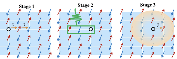
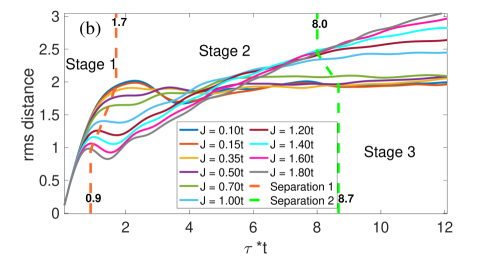
Figure 1: Single-hole dynamics at zero temperature. (a) Sketch of three stages underpinning magnetic polarons emerging from localized defects: (i) kinematic expansion, (ii) polaron formation, and (iii) polaron drift. (b) Evolution of the rms distances $d_{\rm rms}(\tau)$ for spin interaction strengths $J$ indicated in the legend.

We begin with the recapitulation of the hole dynamics at zero temperature. According to the experimental findings ²⁴ and SCBA simulations ³⁰, one can delineate three stages of the hole transport which are sketched in Fig. 1(a): (i) initial kinematic expansion, (ii) emergence of strings and magnetic polarons, and (iii) ballistic low-speed polaron motion. Our mDA-TFD simulations confirm the existence of these three stages. This is illustrated by Fig. 1(b), which displays evolution of the root-mean-square (rms) distances $d_{\rm rms}(\tau)=\sqrt{\sum_{\mathbb{d}}\rho_{h}({\mathbb{d}},\tau)d^{2}}$ for a range of spin interaction strengths $J$. In agreement with Ref. ³⁰, the slope of $d_{\rm rms}(\tau)$ during the ballistic stage (i) deviates from the ideal value of $2t$ owing to interactions with spins. The timescale of this stage, $\tau_{(i)}$, is proportional to $1/t$ in the strong-coupling regime ($J\ll t$), while $\tau_{(i)}\sim 1/J$ in the weak-coupling regime ($J\gg t$). For $J/t=0.1$ and $J/t=1.8$, for example, the initial ballistic motion ceases at $\tau\approx 1.7/t$ and $\tau\approx 0.9/t$, respectively. Stage (ii) is governed by the interference of strings (which correspond to higher-energy states in the hole spectral density) and polarons (which correspond to lower-energy states in the hole spectral density) ^{11, 63}. The stage (ii) terminates at $\tau\approx 8.7/t$ and $\tau\approx 8.0/t$ for $J/t=0.1$ and $J/t=1.8$, respectively, where the corresponding transition time scales as $J/t$ for weak interactions and $(J/t)^{\frac{-2}{3}}$ for strong couplings ³⁰. This delineates the dynamic transition culminating in the eventual propagation of magnons during stage (iii) characterized by the time interval $\tau_{(iii)}$.

The values of $\tau_{(i)}$ and $\tau_{(iii)}$ are determined by the competition between two processes. When the hole travels a displacement that spans an integral number $l$ of lattice constants, the spins subsequently arrange into a pattern incongruous with the Neel state. This deviation from the AFM norm elevates system’s exchange energy by a magnitude on the order of $lJ$. The energetic cost of this disruption effectively inhibits the hole from vacating its initial position, where the Neel order remains undisturbed. Consequently, this energy landscape results in the autolocalization ³⁶ of the hole at a longer time. Basically, a hole placed in a lattice with diminished spin-spin coupling $J$ is likely to traverse further from its primary position prior to the influence exerted by the inherent spin order of the quantum magnet. Nevertheless, a smaller $J$ concurrently signifies a more profound dressing of the hole by spin waves in its final polaron state. For small $J$, the hole dressing wins over the decreased $\sim lJ$ energy penalty in the beginning of stage (ii), preventing the hole from leaving its initial position and pushing it back. This dynamic event is manifested through a pronounced partial recurrence of $d_{\rm rms}(\tau)$ in Fig. 1 (b) which is not grasped by the SCBA method ³⁰. This discrepancy can be attributed to the limitations of SCBA in accurately addressing collective effects and long-range order in strongly correlated systems. A larger $J$ diminishes the dressing effect, causing quenched oscillations in $d_{\rm rms}(\tau)$, the amplitudes of which decrease with $J$. This agrees with predictions of Ref. ³⁰, though SCBA underestimates the oscillation amplitudes in $d_{\rm rms}(\tau)$ in the intermediate regime $t\sim J$ (cf. Ref. ⁶²). Overall, the magnon dressing of the hole significantly decelerates its ballistic expansion in stage (iii) in the strong-coupling regime, leading to the quasi-trapping of the hole. In the weak-coupling regime, the hole moves ballistically in stage (iii)) ($d_{\rm rms}(\tau)\sim\tau$), though much slower than in stage (i).

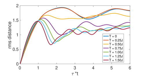
Figure 2: Evolution of the rms distance $d_{\rm rms}(\tau)$ of the hole for $J/t=0.2$ and several temperatures indicated in the legend.

Fig. 2 illustrates how temperature modifies the $d_{\rm rms}(\tau)$ evolution for $J/t=0.2$, a typical value of $J/t$ for high-$T_{\rm c}$ cuprate superconductors ⁹. The three-stage hole-motion scenario remains valid, though with significant temperature-induced modifications at each stage. As $T$ increases, $d_{\rm rms}(\tau)$ exhibits a shorter stage (i), shows earlier reversion of the hole motion and closer returning to the IHS during stage (ii) and demonstrates a slow expansion (quasi-localization) at shorter distances from the IHS during stage (iii). These all phenomena signify the magnetic polaron effect, which is responsible for the effective reduction of the hole-hole couplings with temperature and the ensuing suppression of the hole tunneling. Semi-quantitatively, the coupling decreases $\sim\sum_{\mathbb{q}^{\prime}\mathbb{q}^{\prime\prime}}\xi^{\mathbb{k}\mathbb{q}}_{\mathbb{q}^{\prime}\mathbb{q}^{\prime\prime}}\exp(-\coth\{(\omega_{\mathbb{q}^{\prime}}+\omega_{\mathbb{q}^{\prime\prime}})/(2T)\})$ where $\xi^{\mathbb{k}\mathbb{q}}_{\mathbb{q}^{\prime}\mathbb{q}^{\prime\prime}}$ are determined by the parameters of the model Hamiltonian ^{64, 65}. Interestingly, Monte Carlo simulations of the hole transport in the $t\text{-}J_{z}$ model related to the anisotropic spin-spin interaction in the same (strong-coupling) regime yield qualitatively similar oscillatory evolutions of $d_{\rm rms}(\tau)$ but demonstrate the opposite trend, predicting that the long-time value of $d_{\rm rms}(\tau)$ increases with temperature ⁶⁶. This may be caused by diminished quantum interference effects in the $t\text{-}J_{z}$ model, in which Heisenberg couplings between spins are replaced with Ising couplings.

*

*

*

*

*

*

*

Figure 3: Magnon population dynamics at zero temperature. Panels (a)-(d) and (e)-(h) give 2D views of magnon populations in the $8\times 8$ site space for $J/t=0.10$ and $J/t=1.80$, respectively. Panel (i) shows IHS magnon populations while panel (j) shows NN (full lines) and NNN (dashed lines) magnon populations for spin-spin couplings $J/t$ indicated in the legend. (k) The difference $\Delta$ between the averaged NN and NNN magnon populations (Eq. (4)) as a function of spin-spin coupling $J/t$.

[]  []  []  []
[]  []  []  []

*

The mDA methodology is capable of delivering hole and spin evolutions in the site space as well as in the momentum space – all these observables can be directly computed through mDA wave functions of Eq. (S5) by adopting basis set transformations (see Supporting Information). For example, a direct visualization of the transport pathways is provided by magnon populations in the site basis, which are calculated as $\rho_{m}(\mathbb{d},\tau)=\langle D_{2}^{M}(\tau)|b_{\mathbb{d}}^{\dagger}b_{\mathbb{d}}|D_{2}^{M}(\tau)\rangle$, where $b_{\mathbb{d}}^{\dagger}$ and $b_{\mathbb{d}}$ are obtained from $b_{\mathbb{q}}^{\dagger}$ and $b_{\mathbb{q}}$ by the unitary rotation. $\rho_{m}(\mathbb{d},\tau)$ can be used for the construction of several coarse-grained magnon populations $\rho_{m}(d,\tau)$, where $d=0,\,1,\,\sqrt{2},\,2$ correspond to IHS, NNs, NNNs, and SNNs, respectively.

Magnon dynamics at zero temperature is presented in Fig. 3. Panels (a)-(d) and (e)-(h) elucidate mechanisms of magnon diffusion in real space, giving stroboscopic view of the site populations at $\tau=3j/t$, $j=1,2,3,4$. For weak spin-spin interactions (panels (a)-(d)) magnons spread only over NNs on the timescale $\tau=12/t$. The magnon confinement within the NN area is caused by the hole dressing, as discussed above. Strong spin-spin coupling (panels (e)-(h)) facilitates magnon movements, allowing for magnon diffusion through NNs at intermediate times (panels (e, f)), and to NNNs at longer times (panels (g, h)). Panels (i) and (j) provide another perspective of the diffusion process, highlighting competition between the IHS, NN and NNN populations. Panel (i) shows IHS populations $\rho_{m}(0,\tau)$ which, after a short time $\sim\tau_{(i)}$, attains values around 0.85, 0.8, and 0.5 for $J/t=0.10$, $0.70$, and $1.8$, respectively. Then $\rho_{m}(0,\tau)$ evolves in the oscillatory manner, mirroring magnon population exchanges between the IHS, NN, and NNN areas. Owing to the hole dressing for $J/t=0.1$, $\rho_{m}(0,\tau)$ remains high and even grows slowly at $\tau>5/t$. As demonstrated by the magnon populations in panel (j), for intermediate ($J/t=0.7$) and strong ($J/t=1.8$) spin-spin interactions, $\rho_{m}(0,\tau)$ quenches which is tantamount to the population transfer to the NN and NNN areas. For weak spin-spin interactions ($J/t=0.1$), NN magnon populations remain larger than their NNN counterparts up to $\tau=12/t$, signifying magnon confinement within the NN domain. For $J/t=0.7$, magnon populations in the NNN area surpass those in the NN area up to $\tau\approx 2/t$, while the two populations become comparable at longer times. For strong spin-spin interactions ($J/t=1.8$), on the other hand, the NNN populations outgrow their NN counterparts after $\tau\approx 1/t$. The physical picture of the magnon transport outlined above is further corroborated by panel (h), which displays the averaged difference between the NN and the NNN populations,

$$\Delta=\tau_{f}^{-1}\int_{0}^{\tau_{f}}d\tau\left(\rho_{m}(1,\tau)-\rho_{m}(\sqrt{2},\tau)\right),$$ (4)

as a function of the spin-spin coupling $J/t$, where $\tau_{f}=12/t$. The NN populations dominate for small $J/t$, with $J/t\approx 0.88$ marking a crossover, above which the NNN populations take over.

*

*

*

*

*

*

*

[]  []  []  []
[] []  []  []

*

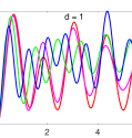
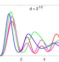
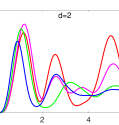
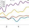
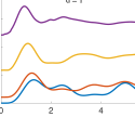
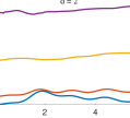
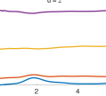
Figure 4: Hole (panels (a-d)) and magnon (panels (e-h)) populations in the IHS, NNs, NNNs, and SNNs areas for elevated temperatures and $J/t=0.2$.

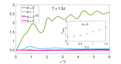
Figure 5: Magnon populations in the IHS, NNs, NNNs, and SNNs areas for $T/J=1.5$ and $J/t=0.2$. Inset shows the average IHS magnon population vs. temperature.

The evolution of hole populations $\rho_{h}(d,\tau)$ (up row) and magnon populations $\rho_{m}(d,\tau)$ (bottom row) in time is elucidated in Fig. 4 for elevated temperatures. From left to right, the panels correspond to IHS ($d=0$), NN ($d=1$), NNN ($d=\sqrt{2}$) and SNN ($d=2$). We begin with general observations. Hole populations exhibit pronounced oscillations at $T=0$ (which correlates, e.g., with the tensor-network calculations ⁶⁷) and elevated temperatures. Remarkably, the amplitudes and periods of oscillations in the IHS (a) and NN (b) hole populations increase with temperature. This is a manifestation of the $T$-enhanced hole-hole coupling caused by the increasing number of thermally-activated magnon states controlling the coupling. In the effective Rabi-model picture, the enhanced coupling amplifies Rabi frequency governing hole-hole population transfer. Similar (though significantly mitigated) effects are observed for magnon populations (e, f). For NNN and SNN hole (c, d) and magnon (g, h) populations, there is no clear trend in the $T$-induced modifications of the amplitudes and the oscillation periods, as long-range, magnon-assisted transfer of holes is inevitably accompanied by multiple forward-backward scatterings in the IHS, NN, NNN, and SNN areas which induces dephasing.

The IHS hole populations in Fig. 4(a) exhibit pronounced recurrences, the amplitude (the period) of which increases (decreases) with temperature – in full agreement with the behavior of rms distances $d_{\rm rms}(\tau)$ in Fig. 2. The NN hole population dynamics (panel (b)) shows a similar pattern. NNN (c) and SNN (d) hole populations exhibit irreversible $T$-induced quenching. Magnon populations (e)-(h), on the other hand, reveal two important general trends. First, $\rho_{m}(d,\tau)$ increases with temperature, mirroring thermal activation of magnons. Second, except for $\rho_{m}(0,\tau)$, magnon populations rapidly attain their steady-state values, notably at higher $T$. This is attributed to destructive quantum interference among multiple thermally-populated magnon states.

The typical values of magnon populations $\rho_{m}(d,\tau)$, in the IHS ($d=0$), NN ($d=1$), NNN ($d=\sqrt{2}$) and SNN ($d=2$) areas at $T=1.5J$, are depicted in Fig. 5. Clearly, the IHS population is higher than the remaining three populations taken together. The inset shows that the averaged IHS magnon population $\rho_{ave}=\tau_{f}^{-1}\int_{0}^{\tau_{f}}d\tau\rho_{m}(0,\tau)$ increases monotonically with $T$. This can be interpreted as thermally-induced frustration of the spin alignment and correlates with the decrement of saturation magnetization at elevated temperatures ^{68, 69}.

In summary, we have elaborated a computationally-efficient, numerically-accurate mDA-TFD methodology for simulating hole-magnon dynamics of the $t\text{-}J$ model at finite temperatures. This permits one to scrutinize previous SCBA predictions ³⁰ while offering, for the first time, finite-temperature calculations of detailed magnon dynamics as a response and a facilitator to the hole motion. Our study also uncovers pronounced $T$-dependence of the magnon and hole populations, pointing to the feasibility of potential thermal manipulation and control of hole dynamics. Time evolutions of magnon populations computed here can be measured by the micro-focus Brillouin light scattering (BLS) spectroscopy ^{70, 71}. Furthermore, our methodology can be applied not only to the calculation of steady-state angular-resolved photoemission spectra ^{72, 73}, but also to the simulation of femtosecond terahertz pump-probe and other nonlinear signals that have been used for the characterization of AFM materials ⁷⁴, as it has been repeatedly shown that the mDA method is a reliable approach to nonlinear time- and frequency-resolved spectra of various material systems ^{10, 11, 9, 76}. It seems especially promising to compare predictions of our simulations on magnon dynamics with measurements of femtosecond terahertz 2D spectroscopy, which is capable of monitoring inter-magnon temporal and spacial correlations ^{77, 78}. In addition, the mDA-TFD framework holds the potential to extend its application to an analysis of magnon polaritons ⁷⁹, AFM bilayers ³², and nonequilibrium dynamics of multiple holes ^{31, 19, 16} in strongly interacting lattice models. Such extensions could foster a more nuanced comprehension of the interplay between holes, magnons, and polarons, and further illuminate fascinating phenomena such as d-wave Cooper pairs, stripe phases, and d-wave superconductivity.

Data Availability Statement

The data that support the findings of this study are available from the corresponding author upon reasonable request.

Supporting Information

The following file is available free of charge.

• supp_v5: The thermo-field dynamics approach, variational equations of motion based on the multi-D2 Ansatz for the $t\text{-}J$ model

Supporting Information: Finite-Temperature Hole-Magnon Dynamics in an Antiferromagnet

Appendix A S1. The thermo-field dynamics approach

The finite temperature effects can be simulated by introducing the additional ”tilde” magnon degrees of freedom $\tilde{\bf q}$ ^{1, 2, 3}. Then the total Hamiltonian acting in the extended $\{\bf q\}=\bf q\oplus\tilde{\bf q}$ Hilbert space assumes the form ⁴

$$\overline{H}=H-\sum_{\bf q}\omega_{\bf q}\tilde{b}_{\bf q}^{\dagger}\tilde{b}_{\bf q}$$ (S1)

where $\tilde{b}_{\bf q}^{\dagger}$ and $\tilde{b}_{\bf q}$ are the tilde creation and annihilation operators. Having performed thermal Bogoliubov transformation specified by the operator

$$G=G^{\dagger}=-i\sum_{\bf q}\theta_{\bf q}(b_{\bf q}\tilde{b}_{\bf q}-b_{\bf q}^{\dagger}\tilde{b}_{\bf q}^{\dagger})$$ (S2)

and following the prescriptions of Refs ^{4, 5}, we obtain the final thermo-field dynamics $t\text{-}J$ Hamiltonian

$$H_{\theta} =e^{iG}\overline{H}e^{-iG}$$

$$=\sum_{\mathbf{q}}\omega_{\mathbf{q}}(b_{\mathbf{q}}^{\dagger}b_{\mathbf{q}}-\tilde{b}_{\mathbf{q}}^{\dagger}\tilde{b}_{\mathbf{q}})+\frac{tz}{\sqrt{N}}\sum_{\mathbf{kq}}h_{\mathbf{k-q}}^{\dagger}h_{\mathbf{k}}\cosh(\theta_{\mathbf{q}})[(u_{\mathbf{q}}\gamma_{\mathbf{k-q}}+v_{\mathbf{q}}\gamma_{\mathbf{k}})b_{\mathbf{q}}^{\dagger}+(u_{\mathbf{q}}\gamma_{\mathbf{k}}+v_{\mathbf{q}}\gamma_{\mathbf{k-q}})b_{\mathbf{-q}}]$$

$$+\frac{tz}{\sqrt{N}}\sum_{\mathbf{kq}}h_{\mathbf{k-q}}^{\dagger}h_{\mathbf{k}}\sinh(\theta_{\mathbf{q}})[(u_{\mathbf{q}}\gamma_{\mathbf{k-q}}+v_{\mathbf{q}}\gamma_{\mathbf{k}})\tilde{b}_{\mathbf{q}}+(u_{\mathbf{q}}\gamma_{\mathbf{k}}+v_{\mathbf{q}}\gamma_{\mathbf{k-q}})\tilde{b}_{\mathbf{-q}}^{\dagger}].$$ (S3)

The influence of temperature is imprinted into $\overline{H}_{\theta}$ through the temperature-dependent mixing angles

$$\theta_{\bf q}={\rm arctanh}(e^{-\beta\omega_{\bf q}/2})$$ (S4)

which renormalize hole-magnon coupling coefficients.

Appendix B S2. Multi-$\rm D_{2}$ ansatz and its variational equations

The multi-$\rm D_{2}$ Ansatz ^{6, 7, 8, 9, 10, 11} of multiplicity $M$ in the thermo-field dynamics method can be constructed as

$$|D_{2}^{\rm M}(\tau)\rangle=\sum_{\scriptstyle 1\leq n\leq N\atop\scriptstyle 1\leq m\leq M}A_{nm}(\tau)|n\rangle{\rm e}^{\sum_{\bf q}(f_{m{\bf q}}(\tau)b_{\bf q}^{\dagger}-{\rm{H.C.}})}|\bf 0\rangle\times{\rm e}^{\sum_{\tilde{\bf q}}(\tilde{f}_{m{\tilde{\bf q}}}(\tau)\tilde{b}_{\tilde{\bf q}}^{\dagger}-{\rm{H.C.}})}\tilde{|\bf 0\rangle}$$ (S5)

where $|n\rangle$ numbers the hole states and $f_{m{\bf q}}$ ($\tilde{f}_{m{\tilde{\bf q}}}$) denote the displacement of the magnon mode with momentum $\bf q$ ($\tilde{\bf q}$) in the $m$th coherent state, and $|\bf 0\rangle$ ($|\tilde{\bf 0}\rangle$) are the vacuum states for the “physical” and “tilde” magnon degrees of freedom.

The time-dependence of the variational parameters $A_{nm}(\tau)$, $f_{m{\bf q}}(\tau)$ and $\tilde{f}_{m{\tilde{\bf q}}}(\tau)$ is determined via the variational principle ^{10, 11}

$$\frac{d}{dt}\frac{\partial\mathcal{L}}{\partial\dot{\xi}_{j}^{\ast}}-\frac{\partial\mathcal{L}}{\partial\xi_{j}^{\ast}}=0,$$ (S6)

where the Lagrangian $\mathcal{L}$ is given by

$$\mathcal{L} = \frac{i}{2}\left[\langle{\rm D}_{2}^{M}(\tau)|\frac{\overrightarrow{\partial}}{\partial\tau}|{\rm D}_{2}^{M}(\tau)\rangle-\langle{\rm D}_{2}^{M}(\tau)|\frac{\overleftarrow{\partial}}{\partial\tau}|{\rm D}_{2}^{M}(\tau)\rangle\right]-\langle{\rm D}_{2}^{M}(\tau)|{H_{\theta}}|{\rm D}_{2}^{M}(\tau)\rangle.$$ (S7)

Appendix C S3. Equations of motion for t-J model at finite temperature

The Hamiltonian in the multi-$\rm D_{2}$ Ansatz is defined as

$$L_{H_{\theta}} =\langle D_{2}^{\rm M}(\tau)|H_{\theta}|D_{2}^{\rm M}(\tau)\rangle=\sum_{n}\sum_{j}^{M}\sum_{u}^{M}A_{nj}^{\ast}A_{nu}\sum_{\bf q}\omega_{\bf q}(f_{j\bf q}^{\ast}f_{u\bf q}-\tilde{f}_{j\bf q}^{\ast}\tilde{f}_{u\bf q})R(f_{j}^{\ast},f_{u})$$

$$+\frac{tz}{\sqrt{N}}\sum_{\bf{kq}}\sum_{j}^{M}\sum_{u}^{M}A_{{\bf(k-q)}j}^{\ast}A_{{\bf(k)}u}[{\rm cosh}(\theta_{\bf q})(u_{\bf q}\gamma_{\bf{k-q}}+v_{\bf q}\gamma_{\bf k})f_{j{\bf q}}^{\ast}+{\rm sinh}(\theta_{\bf q})(u_{\bf q}\gamma_{\bf{k-q}}+v_{\bf q}\gamma_{\bf k})\tilde{f}_{u{\bf q}}]R(f_{j}^{\ast},f_{u})$$

$$+\frac{tz}{\sqrt{N}}\sum_{\bf{kq}}\sum_{j}^{M}\sum_{u}^{M}A_{{\bf(k+q)}j}^{\ast}A_{{\bf(k)}u}[{\rm cosh}(\theta_{\bf q})(u_{\bf{q}}\gamma_{\bf{k}}+v_{\bf{q}}\gamma_{\bf{k+q}})f_{u{\bf q}}+{\rm sinh}(\theta_{\bf q})(u_{\bf{q}}\gamma_{\bf{k}}+v_{\bf{q}}\gamma_{\bf{k+q}})\tilde{f}_{j{\bf q}}^{\ast}]R(f_{j}^{\ast},f_{u})$$

where

$$R(f_{j}^{\ast},f_{u})={\rm{exp}}[\sum_{l}f_{jl}^{\ast}(\tau)f_{ul}(\tau)+\sum_{l}\tilde{f}_{jl}^{\ast}(\tau)\tilde{f}_{ul}(\tau)]$$

is the Debye-Waller factor.

Thus the equation of motion for $A_{nu}$ assumes the form

$$i\sum_{n}\sum_{u}^{M}[\dot{A}_{nu}+A_{nu}\sum_{l}f_{jl}^{\ast}\dot{f}_{ul}+A_{nu}\sum_{l}\tilde{f}_{jl}^{\ast}\tilde{\dot{f}}_{ul}]R(f_{j}^{\ast},f_{u})$$

$$=\sum_{u}^{M}A_{nu}\sum_{\bf q}\omega_{\bf q}(f_{j\bf q}^{\ast}f_{u\bf q}-\tilde{f}_{j\bf q}^{\ast}\tilde{f}_{u\bf q})R(f_{j}^{\ast},f_{u})$$

$$+\frac{tz}{\sqrt{N}}\sum_{\bf{kq,k-q=n}}\sum_{u}^{M}A_{{\bf(k)}u}[{\rm cosh}(\theta_{\bf q})(u_{\bf q}\gamma_{\bf{n}}+v_{\bf q}\gamma_{\bf k})f_{j{\bf q}}^{\ast}+{\rm sinh}(\theta_{\bf q})(u_{\bf q}\gamma_{\bf{n}}+v_{\bf q}\gamma_{\bf k})\tilde{f}_{u{\bf q}}]R(f_{j}^{\ast},f_{u})$$

$$+\frac{tz}{\sqrt{N}}\sum_{\bf{kq,k+q=n}}\sum_{u}^{M}A_{{\bf(k)}u}[{\rm cosh}(\theta_{\bf q})(u_{\bf{q}}\gamma_{\bf{k}}+v_{\bf{q}}\gamma_{\bf{n}})f_{u{\bf q}}+{\rm sinh}(\theta_{\bf q})(u_{\bf{q}}\gamma_{\bf{k}}+v_{\bf{q}}\gamma_{\bf{n}})\tilde{f}_{j{\bf q}}^{\ast}]R(f_{j}^{\ast},f_{u})$$ (S9)

Similarly, the equations of motion for $f_{ul}$ and $\tilde{f}_{ul}$ are given by the formulas

$$i\sum_{n}\sum_{u}^{M}A_{nj}^{\ast}A_{nu}\dot{f}_{ul}R(f_{j}^{\ast},f_{u})+i\sum_{n}\sum_{u}^{M}[A_{nj}^{\ast}\dot{A}_{nu}+A_{nj}^{\ast}A_{nu}(\sum_{l}f_{jl}^{\ast}\dot{f}_{ul}+\sum_{l}\tilde{f}_{jl}^{\ast}\tilde{\dot{f}}_{ul})]R(f_{j}^{\ast},f_{u})f_{ul}$$

$$=\sum_{n}\sum_{u}^{M}A_{nj}^{\ast}A_{nu}\sum_{\bf q}\omega_{\bf q}(f_{j\bf q}^{\ast}f_{u\bf q}-\tilde{f}_{j\bf q}^{\ast}\tilde{f}_{u\bf q})R(f_{j}^{\ast},f_{u})f_{ul}+\sum_{m}\sum_{u}^{M}A_{nj}^{\ast}A_{nu}\omega_{\bf l}f_{u\bf l}R(f_{j}^{\ast},f_{u})$$

$$+\frac{tz}{\sqrt{N}}\sum_{\bf{kq}}\sum_{u}^{M}A_{{\bf(k-q)}j}^{\ast}A_{{\bf(k)}u}[{\rm cosh}(\theta_{\bf q})(u_{\bf q}\gamma_{\bf{k-q}}+v_{\bf q}\gamma_{\bf k})f_{j{\bf q}}^{\ast}+{\rm sinh}(\theta_{\bf q})(u_{\bf q}\gamma_{\bf{k-q}}+v_{\bf q}\gamma_{\bf k})\tilde{f}_{u{\bf q}}]R(f_{j}^{\ast},f_{u})f_{ul}$$

$$+\frac{tz}{\sqrt{N}}\sum_{\bf{kq}}\sum_{u}^{M}A_{{\bf(k-q)}j}^{\ast}A_{{\bf(k)}u}[{\rm cosh}(\theta_{\bf q})(u_{\bf{q}}\gamma_{\bf{k}}+v_{\bf{q}}\gamma_{\bf{k+q}})f_{u{\bf q}}+{\rm sinh}(\theta_{\bf q})(u_{\bf{q}}\gamma_{\bf{k}}+v_{\bf{q}}\gamma_{\bf{k+q}})\tilde{f}_{j{\bf q}}^{\ast}]R(f_{j}^{\ast},f_{u})f_{ul}$$

$$+\frac{tz}{\sqrt{N}}\sum_{\bf{k}}\sum_{u}^{M}A_{{\bf(k-l)}j}^{\ast}A_{{\bf(k)}u}[{\rm cosh}(\theta_{\bf l})(u_{\bf l}\gamma_{\bf{k-l}}+v_{\bf l}\gamma_{\bf k})R(f_{j}^{\ast},f_{u})$$ (S10)

and

$$i\sum_{n}\sum_{u}^{M}A_{nj}^{\ast}A_{nu}\tilde{\dot{f}}_{ul}R(f_{j}^{\ast},f_{u})+i\sum_{n}\sum_{u}^{M}[A_{nj}^{\ast}\dot{A}_{nu}+A_{nj}^{\ast}A_{nu}(\sum_{l}f_{jl}^{\ast}\dot{f}_{ul}+\sum_{l}\tilde{f}_{jl}^{\ast}\tilde{\dot{f}}_{ul})]R(f_{j}^{\ast},f_{u})\tilde{f}_{ul}$$

$$=\sum_{n}\sum_{u}^{M}A_{nj}^{\ast}A_{nu}\sum_{\bf q}\omega_{\bf q}(f_{j\bf q}^{\ast}f_{u\bf q}-\tilde{f}_{j\bf q}^{\ast}\tilde{f}_{u\bf q})R(f_{j}^{\ast},f_{u})\tilde{f}_{ul}-\sum_{n}\sum_{u}^{M}A_{nj}^{\ast}A_{nu}\omega_{\bf l}\tilde{f}_{u\bf l}R(f_{j}^{\ast},f_{u})$$

$$+\frac{tz}{\sqrt{N}}\sum_{\bf{kq}}\sum_{u}^{M}A_{{\bf(k-q)}j}^{\ast}A_{{\bf(k)}u}[{\rm cosh}(\theta_{\bf q})(u_{\bf q}\gamma_{\bf{k-q}}+v_{\bf q}\gamma_{\bf k})f_{j{\bf q}}^{\ast}+{\rm sinh}(\theta_{\bf q})(u_{\bf q}\gamma_{\bf{k-q}}+v_{\bf q}\gamma_{\bf k})\tilde{f}_{u{\bf q}}]R(f_{j}^{\ast},f_{u})\tilde{f}_{ul}$$

$$+\frac{tz}{\sqrt{N}}\sum_{\bf{kq}}\sum_{u}^{M}A_{{\bf(k+q)}j}^{\ast}A_{{\bf(k)}u}[{\rm cosh}(\theta_{\bf q})(u_{\bf{q}}\gamma_{\bf{k}}+v_{\bf{q}}\gamma_{\bf{k+q}})f_{u{\bf q}}+{\rm sinh}(\theta_{\bf q})(u_{\bf{q}}\gamma_{\bf{k}}+v_{\bf{q}}\gamma_{\bf{k+q}})\tilde{f}_{j{\bf q}}^{\ast}]R(f_{j}^{\ast},f_{u})\tilde{f}_{ul}$$

$$+\frac{tz}{\sqrt{N}}\sum_{\bf{k}}\sum_{u}^{M}A_{{\bf(k+l)}j}^{\ast}A_{{\bf k}u}[{\rm sinh}(\theta_{\bf l})(u_{\bf{l}}\gamma_{\bf{k}}+v_{\bf{l}}\gamma_{\bf{k+l}})R(f_{j}^{\ast},f_{u})$$ (S11)

The magnon population in site $\bf d$ is expressed as

$$N_{\bf d}(\tau) =\langle D_{2}^{M}(\tau)|e^{iG}b_{\bf d}^{\dagger}b_{\bf d}e^{-iG}|D_{2}^{M}(\tau)\rangle$$

$$=\langle D_{2}^{M}(\tau)|\frac{1}{N}\sum_{\bf{q_{1}q_{2}}}e^{-i(\bf{q_{1}-q_{2}}){\bf d}}e^{iG}b_{\bf q_{1}}^{\dagger}b_{\bf q_{2}}e^{-iG}|D_{2}^{M}(\tau)\rangle$$

$$=\langle D_{2}^{M}(\tau)|\frac{1}{N}\sum_{\bf{q_{1}q_{2}}}e^{-i(\bf{q_{1}-q_{2}}){\bf d}}[{\rm cosh}(\theta_{\bf q1}){\rm cosh}(\theta_{\bf q2})b_{\bf q_{1}}^{\dagger}b_{\bf q_{2}}+{\rm cosh}(\theta_{\bf q1}){\rm sinh}(\theta_{\bf q2})b_{\bf q_{1}}^{\dagger}\tilde{b}_{\bf q_{2}}^{\dagger}$$

$$+{\rm sinh}(\theta_{\bf q1}){\rm cosh}(\theta_{\bf q2})\tilde{b}_{\bf q_{1}}{b}_{\bf q_{2}}+{\rm sinh}(\theta_{\bf q1}){\rm sinh}(\theta_{\bf q2})\tilde{b}_{\bf q_{1}}\tilde{b}_{\bf q_{2}}^{\dagger}]|D_{2}^{M}(\tau)\rangle$$

$$=\frac{1}{N}\sum_{\bf{q_{1}q_{2}}}e^{-i(\bf{q_{1}-q_{2}}){\bf d}}\sum_{n}\sum_{j,u}^{M}A_{nj}^{\ast}A_{nu}[f_{j(\bf q_{1})}^{\ast}(\tau)f_{u(\bf q_{2})}(\tau){\rm cosh}(\theta_{\bf q1}){\rm cosh}(\theta_{\bf q2})$$

$$+f_{j(\bf q_{1})}^{\ast}(\tau)\tilde{f}_{j(\bf q_{2})}^{\ast}(\tau){\rm cosh}(\theta_{\bf q1}){\rm sinh}(\theta_{\bf q2})+\tilde{f}_{u(\bf q_{1})}(\tau){f}_{u(\bf q_{2})}(\tau){\rm sinh}(\theta_{\bf q1}){\rm cosh}(\theta_{\bf q2})$$

$$+\tilde{f}_{j(\bf q_{2})}^{\ast}(\tau)\tilde{f}_{u(\bf q_{1})}(\tau){\rm sinh}(\theta_{\bf q1}){\rm sinh}(\theta_{\bf q2})]R(f_{j}^{\ast},f_{u})+\frac{1}{N}\sum_{\bf{q_{1}}}\sum_{n}\sum_{j,u}^{M}A_{nj}^{\ast}A_{nu}{\rm sinh}^{2}(\theta_{\bf q1})R(f_{j}^{\ast},f_{u})$$ (S12)

References

- 1 Nagaev, E. L. Ferromagnetic and antiferromagnetic semiconductors. Sov. Phys. Usp. 1975,18, 863.
- 2 Schmitt-Rink, S.; Varma, C. M.; Ruckenstein, A. E. Spectral Function of Holes in a Quantum Antiferromagnet. Phys. Rev. Lett. 1988, 60, 2793.
- 3 Shraiman, B. I.; Siggia, E. D. Mobile Vacancies in a Quantum Heisenberg Antiferromagnet. Phys. Rev. Lett. 1988, 61, 467.
- 4 Kane, C. L.; Lee, P. A.; Read, N. Motion of a single hole in a quantum antiferromagnet. Phys. Rev. B. 1989, 39, 6880.
- 5 Sachdev, S. Hole motion in a quantum Néel state. Phys. Rev. B. 1989, 39, 12232.
- 6 Trugman, S. A. Spectral function of a hole in a Hubbard antiferromagnet. Phys. Rev. B. 1990, 41, 892.
- 7 Liu, Z.; Manousakis, E. Dynamical properties of a hole in a Heisenberg antiferromagnet. Phys. Rev. B. 1992, 45, 2425.
- 8 Dagotto, E. Correlated electrons in high-temperature superconductors. Rev. Mod. Phys. 1994, 66, 763.
- 9 Lee, P. A.; Nagaosa, N.; Wen, X.-G. Doping a Mott insulator: Physics of high-temperature superconductivity. Rev. Mod. Phys. 2006, 78, 17-81.
- 10 Mishchenko, A. S.; Nagaosa, N. Electron-Phonon Coupling and a Polaron in the t-J Model: From the Weak to the Strong Coupling Regime. Phys. Rev. Lett. 2004, 93, 036402.
- 11 Manousakis, E. String excitations of a hole in a quantum antiferromagnet and photoelectron spectroscopy. Phys. Rev. B. 2007, 75, 035106.
- 12 Pirro, P.; Vasyuchka, V. I.; Serga, A. A.; Hillebrands, B. Advances in coherent magnonics. Nat. Rev. Mater. 2021, 6, 1114–1135.
- 13 Boll, M.; Hilker, T. A.; Salomon, G.; Omran, A.; Nespolo, J.; Pollet, L.; Bloch, I.; Gross, C. Spin- and density-resolved microscopy of antiferromagnetic correlations in Fermi-Hubbard chains. Science. 2016, 353, 1257.
- 14 Mazurenko, A.; Chiu, C. S.; Ji, G.; Parsons, M. F.; Kanász-Nagy, M.; Schmidt, R.;Grusdt, F.; Demler, E.; Greif, D.; Greiner, M. A cold-atom Fermi-Hubbard antiferromagnet. Nature. 2017, 545, 462.
- 15 Brown, P. T.; Mitra, D.; Guardado-Sanchez, E.; Schauß, P.; Kondov, S. S.; Khatami, E.; Paiva, T.; Trivedi, N.; Huse, D. A.; Bakr, W. S. Spin-imbalance in a 2D Fermi-Hubbard system. Science. 2017, 357, 1385.
- 16 Chiu, C. S.; Ji, G.; Bohrdt, A.; Xu, M.; Knap, M.; Demler, E.; Grusdt, F.; Greiner, M.; Greif, D. String patterns in the doped Hubbard model. Science. 2019, 365, 251.
- 17 Vijayan, J.; Sompet, P.; Salomon, G.; Koepsell, J.; Hirthe, S.; Bohrdt, A.; Grusdt, F.; Bloch, I.; Gross, C. Time-resolved observation of spin-charge deconfinement in fermionic Hubbard chains. Science. 2020, 367, 186.
- 18 Guardado-Sanchez, E.; Morningstar, A.; Spar, B.M.; Brown, P. T.; Huse, D. A.; Bakr, W. S. Subdiffusion and Heat Transport in a Tilted Two-Dimensional Fermi-Hubbard System. Phys. Rev. X. 2020, 10, 011042.
- 19 Koepsell, J.; Bourgund, D.; Sompet, P.; Hirthe, S.; Bohrdt, A.; Wang, Y.; Grusdt, F.; Demler, E.; Salomon, G.; Gross, C.; Bloch, I. Microscopic evolution of doped Mott insulators from polaronic metal to Fermi liquid. Science. 2021, 374, 82.
- 20 Gall, M.; Wurz, N.; Samland, J.; Chan, C. F.; Köhl, M. Competing magnetic orders in a bilayer Hubbard model with ultracold atoms. Nature (London). 2021, 589, 40.
- 21 Bakr, W. S.; Gillen, J. I.; Peng, A.; Fölling, S.; Greiner, M. A quantum gas microscope for detecting single atoms in a Hubbard-regime optical lattice. Nature (London). 2009, 462, 74.
- 22 Haller, E.; Hudson, J.; Kelly, A.; Cotta, D. A.; Peaudecerf, B.; Bruce, G. D.; Kuhr, S. Single-atom imaging of fermions in a quantum-gas microscope. Nat. Phys. 2015, 11, 738.
- 23 Yang, J.; Liu, L.; Mongkolkiattichai, J.; Schauss, P. Site-Resolved Imaging of Ultracold Fermions in a Triangular-Lattice Quantum Gas Microscope. PRX Quantum. 2021, 2, 020344.
- 24 Ji, G.; Xu, M.; Kendrick, L. H.; Chiu, C. S.; Brüggenjürgen, J. C.; Greif, D.; Bohrdt, A.; Grusdt, F.; Demler, E.; Lebrat, M.; Greiner, M. Coupling a Mobile Hole to an Antiferromagnetic Spin Background: Transient Dynamics of a Magnetic Polaron. Phys. Rev. X. 2021, 11, 021022.
- 25 Schrieffer, J. R.; Wen, X.-G.; Zhang, S.-C. Spin-bag mechanism of high-temperature superconductivity. Phys. Rev. Lett. 1988, 60, 944.
- 26 Anderson, R.; Wang, F.; Xu, P.; Venu, V.; Trotzky, S.; Chevy, F.; Thywissen, J. H. Conductivity Spectrum of Ultracold Atoms in an Optical Lattice. Phys. Rev. Lett. 2019, 122, 153602.
- 27 Nichols, M. A.; Cheuk, L. W.; Okan, M.; Hartke, T. R.; Mendez, E.; Senthil, T.; Khatami, E.; Zhang, H.; Zwierlein, M. W. Spin Transport in a Mott Insulator of Ultracold Fermions. Science. 2019, 363, 383.
- 28 Ronning, F.; Shen, K. M.; Armitage, N. P.; Damascelli, A.; Lu, D. H.; Shen, Z. X.; Miller, L. L.; Kim, C. Anomalous high-energy dispersion in angle-resolved photoemission spectra from the insulating cuprate Ca2CuO2Cl2. Phys. Rev. B. 2005, 71, 094518.
- 29 Graf, J.; Gweon, G.-H.; McElroy, K.; Zhou, S. Y.; Jozwiak, C.; Rotenberg, E.; Bill, A.; Sasagawa, T.; Eisaki, H.; Uchida, S.; Takagi, H.; Lee, D.-H.; Lanzara, A. Phys. Rev. Lett. 2007, 98, 067004.
- 30 Nielsen, K. K.; Pohl T.; Bruun, G. M. Nonequilibrium Hole Dynamics in Antiferromagnets: Damped Strings and Polarons. Phys. Rev. Lett. 2022, 129, 246601.
- 31 Nielsen, K. K. Exact dynamics of two holes in two-leg antiferromagnetic ladders. Phys. Rev. B. 2023, 108, 085125.
- 32 Nyhegn, J. H.; Bruun, G. M.; Nielsen, K. K. Wave function and spatial structure of polarons in an antiferromagnetic bilayer. Phys. Rev. B. 2023, 108, 075141.
- 33 Kanász-Nagy, M.; Lovas, I.; Grusdt, F.; Greif, D.; Greiner, M.; Demler, E. A. Quantum correlations at infinite temperature: The dynamical Nagaoka effect. Phys. Rev. B. 2017, 96, 014303.
- 34 Tanamoto, T.; Kuboki, K.; Fukuyama, H. Magnetic Properties of t-J Model. J. Phys. Soc. Jap. 1991, 60, 3072-3092.
- 35 Igarashi, J.-I.; Fulde, P. Motion of a single hole in a quantum antiferromagnet at finite temperatures. Phys. Rev. B. 1993, 48, 998-1007.
- 36 Izyumov, Y. A. Strongly correlated electrons: the t-J model. Physics-Uspekhi, 1997, 40, 445.
- 37 Zhao, Y. The hierarchy of Davydov’s Ansätze: From guesswork to numerically “exact” many-body wave functions. J. Chem. Phys. 2023, 158, 080901.
- 38 Zhao, Y.; Sun, K.; Chen, L.; Gelin, M. The hierarchy of Davydov’s Ansätze and its applications. WIREs Comp. Mol. Sci. 2022, 12, e1589.
- 39 Takahashi, Y.; Umezawa, H. Thermo field dynamics. Int. J. Mod. Phys. B. 1996, 10, 1755.
- 40 Suzuki, M. Density Matrix Formalism, Double-Space and Thermo Field Dynamics in Non-Equilibrium Dissipative Systems. Int. J. Mod. Phys. B. 1991, 05, 1821.
- 41 Ramšak, A.; Horsch, P. Spin polarons in the t-J model: Shape and backflow. Phys. Rev. B 1993, 48, 10559.
- 42 Borrelli, R.; Gelin, M. F. WIREs Comput. Mol. Sci. 2021, 11, e1539.
- 43 Wang, L.; Zheng, F.; Wang, J.; Grossmann, F.; Zhao, Y. Schrödinger-Cat States in Landau–Zener–Stückelberg–Majorana Interferometry: A Multiple Davydov Ansatz Approach. J. Phys. Chem. B. 2021, 125, 3184-3196.
- 44 Zheng, F.; Shen, Y.; Sun, K.; Zhao,Y. Photon-assisted Landau-Zener transitions in a periodically driven Rabi dimer coupled to a dissipative mode. J. Chem. Phys. 2021, 154, 044102.
- 45 Sun, K.; Gelin, M. F.; Zhao, Y. Accurate Simulation of Spectroscopic Signatures of Cavity-Assisted, Conical-Intersection-Controlled Singlet Fission Processes. J. Phys. Chem. Lett. 2022, 13, 4280-4288.
- 46 Sun, K.; Gelin, M. F.; Zhao, Y. Engineering Cavity Singlet Fission in Rubrene. J. Phys. Chem. Lett. 2022, 13, 4090-4097.
- 47 Chen, L.; Gelin, M. F.; Domcke, W.; Zhao, Y. Theory of femtosecond coherent double-pump single-molecule spectroscopy:Application to light harvesting complexes. J. Chem. Phys. 2015, 142, 164106.
- 48 Chen, L.; Gelin, M. F.; Domcke, W.; Zhao, Y. Simulation of Femtosecond Phase-Locked Double-Pump Signals of Individual Light Harvesting Complexes LH2. J. Phys. Chem. Lett. 2018, 9, 4488-4494.
- 49 Shen, K.; Sun, K.; Zhao, Y. Simulation of emission spectra of transition metal dichalcogenide monolayers with the multimode brownian oscillator model. J. Phys. Chem. A. 2022, 126, 2706-2715.
- 50 Sun, K.; Shen, K.; Gelin, M. F.; Zhao, Y. Exciton Dynamics and Time-Resolved Fluorescence in Nanocavity-Integrated Monolayers of Transition-Metal Dichalcogenides. J. Phys. Chem. Lett. 2022, 14, 221-229.
- 51 Borrelli, R.; Gelin, M. F. Quantum dynamics of vibrational energy flow in oscillator chains driven by anharmonic interactions. New J. Phys. 2020, 22, 123002.
- 52 Gelin, M. F.; Velardo, A.; Borrelli, R. Efficient quantum dynamics simulations of complex molecular systems: A unified treatment of dynamic and static disorder. J. Chem. Phys. 2021, 155, 134102.
- 53 Gelin, M. F.; Borrelli, R. Thermo-Field Dynamics Approach to Photo-induced Electronic Transitions Driven by Incoherent Thermal Radiation. J. Chem. Theory Comput. 2023, 19, 6402-6413.
- 54 TFD-TT machinery is akin to the time-dependent density matrix renormalization group 55 and other tensor network techniques 56, 57.
- 55 Feiguin, A. E.; White, S. R. Finite-temperature density matrix renormalization using an enlarged Hilbert space. Phys. Rev. B 2005, 72, 220401R.
- 56 Qin, M.; Schäfer, T.; Andergassen, S.; Corboz, P.; Gull, E. The Hubbard model: A computational perspective. Annu. Rev. Condens. Matter Phys. 2022, 13, 275-302.
- 57 Sinha, A.; Rams, M. M.; Czarnik, P.; Dziarmaga, J. Finite-temperature tensor network study of the Hubbard model on an infinite square lattice. Phys. Rev. B 2022, 106, 195105.
- 58 Chen, L.; Zhao, Y. Finite temperature dynamics of a Holstein polaron: The thermo-field dynamics approach. J. Chem. Phys. 2017, 147, 214102.
- 59 Chen, L.; Borrelli, R.; Shalashilin, D. V.; Zhao, Y.; Gelin, M. F. Simulation of time- and frequency-resolved four-wave-mixing signals at finite temperature: a thermo-field dynamics approach. J. Chem. Theory Comput. 2021, 17, 4359-4373.
- 60 Zhao, Y.; Chen, G.; Yu, L. Lattice and Spin Polarons in Two Dimensions. J. Chem. Phys. 2000, 113, 6502–6508.
- 61 Grusdt, F.; Kánasz-Nagy, M.; Bohrdt, A.; Chiu, C. S.; Ji, G.; Greiner, M.; Greif, D.; Demler, E. Parton Theory of Magnetic Polarons: Mesonic Resonances and Signatures in Dynamics. Physical Review X. 2018, 8, 011046.
- 62 Bohrdt, A.; Grusdt, F.; Knap, M. Dynamical formation of a magnetic polaron in a two-dimensional quantum antiferromagnet. New J. Phys. 2020, 22, 123023.
- 63 Diamantis, N. G.; Manousakis, E. Dynamics of string-like states of a hole in a quantum antiferromagnet: a diagrammatic Monte Carlo simulation. New J. Phys. 2021, 23, 123005.
- 64 Munn, R. W.; Silbey, R. Theory of electronic transport in molecular crystals. II. Zeroth order states incorporating nonlocal linear electron–phonon coupling. J. Chem. Phys. 1985, 83, 1843.
- 65 Chen, D.; Ye, J.; Zhang, H.; Zhao, Y. On The Munn-Silbey Approach to Polaron Transport with Off-Diagonal Coupling and Temperature-Dependent Canonical Transformations. J. Phys. Chem. B 2011, 115, 5312-5321.
- 66 Hahn, L.; Bohrdt, A.; Grusdt, F. Dynamical signatures of thermal spin-charge deconfinement in the doped Ising model. Phys. Rev. B 2022, 105, L241113.
- 67 Hubig, C.; Bohrdt, A.; Knap, M.; Grusdt, F.; Cirac, J. I. Evaluation of time-dependent correlators after a local quench in iPEPS: hole motion in the t-J model. SciPost Phys. 2020, 8, 021.
- 68 Pryadko, L. P.; Kivelson, S. A.; Zachar, O. Incipient Order in the t-J Model at High Temperatures. Phys. Rev. Lett. 2004, 92, 067002.
- 69 Olsson, K. S.; An, K.; Li, X. Magnon and phonon thermometry with inelastic light scattering. Journal of Physics D: Applied Physics. 2018, 51, 133001.
- 70 Divinskiy, B.; Merbouche, H.; Demidov, V. E.; Nikolaev, K. O.; Soumah, L.; Gouéré, D.; Lebrun, R.; Cros, V.; Youssef, J. B.; Bortolotti, P.; Anane, A.; Demokritov, S. O. Evidence for spin current driven Bose-Einstein condensation of magnons. Nature communications. 2021, 12, 6541.
- 71 Demidov, V. E.; Demokritov, S. O. Magnonic Waveguides Studied by Microfocus Brillouin Light Scattering. IEEE Transactions on Magnetics. 2015, 51, 1-15.
- 72 Bohrdt, A.; Greif, D.; Demler, E.; Knap, M.; Grusdt, F. Angle-resolved photoemission spectroscopy with quantum gas microscopes. Phys. Rev. B 2018, 97, 125117.
- 73 Bohrdt, A.; Demler, E.; Pollmann, F.; Knap, M.; Grusdt, F. Parton theory of angle-resolved photoemission spectroscopy spectra in antiferromagnetic Mott insulators. Phys. Rev. B 2020, 102, 035139.
- 74 Dong, T.; Zhang, S.-J.; Wang, N.-L. Recent Development of Ultrafast Optical Characterizations for Quantum Materials. Adv. Mater. 2023, 35, 2110068.
- 75 Sun, K.; Xie, W.; Chen, L.; Domcke, W.; Gelin, M. F. Multi-faceted spectroscopic mapping of ultrafast nonadiabatic dynamics near conical intersections: A computational study. J. Chem. Phys. 2020, 153, 174111.
- 76 Sun, K.; Xu, Q.; Chen, L.; Gelin, M. F.; Zhao, Y. Temperature effects on singlet fission dynamics mediated by a conical intersection. J. Chem. Phys. 2020, 153, 194106.
- 77 Lu, J.; Li, X.; Hwang, H. Y.; Ofori-Okai, B. K.; Kurihara, T.; Suemoto, T.; Nelson, K. A. Coherent Two-Dimensional Terahertz Magnetic Resonance Spectroscopy of Collective Spin Waves. Phys. Rev. Lett. 2017, 118, 207204.
- 78 Zhang, J.; Tanimura, Y. Coherent two-dimensional THz magnetic resonance spectroscopies for molecular magnets: Analysis of Dzyaloshinskii-Moriya interaction. J. Chem. Phys. 2023, 159, 014102.
- 79 Kato, K.; Yokoyama, T.; Ishihara, H. Functionalized High-Speed Magnon Polaritons Resulting from Magnonic Antenna Effect. Phys Rev. Applied 2023, 19, 034035.

References

- 1 Takahashi, Y.; Umezawa, H. Thermo field dynamics. Int. J. Mod. Phys. B 1996, 10, 1755.
- 2 Suzuki, M. DENSITY MATRIX FORMALISM, DOUBLE-SPACE AND THERMO FIELD DYNAMICS IN NON-EQUILIBRIUM DISSIPATIVE SYSTEMS. Int. J. Mod. Phys. B. 1991, 05, 1821.
- 3 Suzuki, M. Thermo field dynamics of quantum spin systems. J. Stat. Phys. 1986, 42, 1047.
- 4 Borrelli, R.; Gelin, M. F. Quantum electron-vibrational dynamics at finite temperature: Thermo field dynamics approach. J. Chem. Phys. 2016, 145, 224101.
- 5 Chen, L.; Zhao, Y. Finite temperature dynamics of a Holstein polaron: The thermo-field dynamics approach. J. Chem. Phys. 2017, 147, 214102.
- 6 Zheng, F.; Shen, Y.; Sun, K.; Zhao, Y. Photon-assisted Landau–Zener transitions in a periodically driven Rabi dimer coupled to a dissipative mode. J. Chem. Phys. 2021, 154, 044102.
- 7 Sun, K.; Gelin, M. F.; Zhao, Y. Accurate simulation of spectroscopic signatures of cavity-assisted, conical-intersection-controlled singlet fission processes. J. Phys. Chem. Lett. 2022, 13, 4280-4288.
- 8 Sun, K.; Gelin, M. F.; Zhao, Y. Engineering cavity singlet fission in rubrene. J. Phys. Chem. Lett. 2022, 13, 4090-4097.
- 9 Sun, K.; Shen, K.; Gelin, M.; Zhao, Y. Exciton Dynamics and Time-Resolved Fluorescence in Nanocavity-Integrated Monolayers of Transition-Metal Dichalcogenides. J. Phys. Chem. Lett. 2022, 14, 221-229.
- 10 Zhao, Y.; Sun, K.; Chen, L.; Maxim, G. WIREs Comput. Mol. Sci. 2021, DOI: 10.1002/wcms.1589.
- 11 Zhao, Y. The hierarchy of Davydov’s Ansätze: From guesswork to numerically “exact” many-body wave functions. J. Chem. Phys. 2023, 158, 080901.