IJDS-0001-1922.65
Data-driven Option Pricing
Data-driven Option Pricing111Dai acknowledges the supports of Hong Kong GRF (15217123, 15213422), The Hong Kong Polytechnic University Research Grants (P0039114, P0042456, P0042708, and P0045342), and NSFC (12071333).
Min Daia, Hanqing Jinb, Xi Yangc
aDepartment of Applied Mathematics and School of Accounting and Finance, The Hong Kong Polytechnic University, Kowloon, Hong Kong, \EMAILmindai@polyu.edu.hk; bMathematical Institute, University of Oxford, Andrew Wiles Building, Radcliffe Observatory Quarter, Woodstock Road, Oxford, OX2 6GG, United Kingdom, \EMAILjinh@maths.ox.ac.uk; cDepartment of Mathematics, National University of Singapore, Block S17,10 Lower Kent Ridge Road, Singapore, \EMAILyangxi@u.nus.edu
We propose an innovative data-driven option pricing methodology that relies exclusively on the dataset of historical underlying asset prices. While the dataset is rooted in the objective world, option prices are commonly expressed as discounted expectations of their terminal payoffs in a risk-neutral world. Bridging this gap motivates us to identify a pricing kernel process, transforming option pricing into evaluating expectations in the objective world. We recover the pricing kernel by solving a utility maximization problem, and evaluate the expectations in terms of a functional optimization problem. Leveraging the deep learning technique, we design data-driven algorithms to solve both optimization problems over the dataset. Numerical experiments are presented to demonstrate the efficiency of our methodology.
Option pricing; data-driven; pricing kernel; utility maximization; deep learning
1 Introduction
Black and Scholes (1973) develop the celebrated Black-Scholes option pricing model. However, the constant volatility assumed in the model contradicts the volatility smile phenomenon prevalent in options markets.222See, e.g., Hull (2014). To align with the volatility smile phenomenon, existing literature proposes various advanced option pricing models beyond the Black-Scholes world, such as local volatility models, stochastic volatility models, and jump-diffusion models.333See, e.g., Dupire (1994), Heston (1993), Hull and White (1987), Merton (1976), and Kou (2002). Calibrating these models often requires an ample and reliable dataset of (vanilla) option prices, which is, however, absent in many emerging options markets. For example, there are no exchange-traded options on individual stocks in China. Even in the U.S., only a limited number of exchange-traded options are written on less liquid stocks.
This paper aims to develop a novel data-driven option pricing methodology exclusively reliant on historical underlying asset prices. This pricing methodology dispenses with a routine calibration step that involves market prices of options, and as a consequence, it can apply to derivatives pricing in emerging derivatives markets. Our methodology shares similarities with the deep hedging method (e.g., Buehler et al. 2019), both utilizing the deep learning technique and historical underlying asset prices. However, unlike the deep hedging method, which finds risk-indifference prices of a derivative, our methodology instead finds a pricing kernel that links the objective probability measure to a risk-neutral probability measure. The pricing kernel enables us to price any derivatives on the (same) underlying asset by evaluating an expectation in the objective probability measure via historical underlying asset prices.
Next we elaborate on our data-driven pricing methodology. For illustration, we assume that our data is the historical underlying asset prices generated by an Ito process, where the drift and volatility terms are unknown deterministic functions of the underlying asset price. Crucially, these terms are presumed to be time-independent as our methodology attempts to extract the price information of options solely from our dataset.
While our dataset is rooted in the objective world, option prices are commonly expressed as discounted expectations of their terminal payoffs in the risk-neutral world. Bridging this gap via a data-driven method motivates us to identify a pricing kernel process, transforming option pricing into estimating expectations in the objective world. Our key idea is to introduce a dynamic logarithmic utility optimization problem whose optimal wealth process turns out to be the reciprocal of the pricing kernel process. The utility optimization problem naturally induces a loss function, which can be evaluated over the sample paths drawn from our dataset. Minimizing the loss function leads to the optimal wealth process, or equivalently, the pricing kernel process.
Once the pricing kernel process is available, pricing a derivative is then reduced to estimating the expectation of its terminal payoff multiplied by the pricing kernel in the objective world. Inspired by Jia and Zhou (2022), we estimate the expectation by minimizing a martingale loss function, which is also evaluated over our dataset.
Leveraging the deep learning technique, we design data-driven algorithms to minimize the loss functions over our dataset. As a learning algorithm usually requires a huge amount of data and our method uses historical data of underlying asset prices rather than simulated data, we have to allow overlapping sample paths. As such, the initial prices of different sample paths differ in general. Assuming time-homogeneity of market parameters, we rephrase our optimization problems to exclude the dependence on the initial prices of sample paths, and the minimizers we try to find are functions of the underlying asset price. We present numerical experiments to demonstrate the efficiency of our algorithms.
Related Literature.
Recently, data-driven option pricing methods have attracted much research interest. Instead of specifying a particular underlying market model, these methods make mild assumptions about the market and directly utilize the dataset of historical prices. One example is a deep hedging method proposed by Buehler et al. (2019), who utilize a deep learning technique for risk-indifference pricing and hedging of derivatives in frictional markets. Our approach differs significantly from this method in two primary aspects. First, our approach builds on the martingale theory of derivatives pricing. As such, the derivative prices obtained from our approach are theoretically arbitrage-free and interpretable. In contrast, arbitrage opportunities may exist among derivative prices derived from deep hedging. Second, the deep hedging method necessitates separate training for different derivatives on the same underlying. In contrast, our approach conducts a single training phase to estimate the pricing kernel that applies to all derivatives on the same underlying, thereby reducing the amount of computation significantly.
To construct the pricing kernel, we introduce a dynamic portfolio optimization problem. There is rich literature on data-driven portfolio optimization with reinforcement learning. For example, Wang et al. (2020) propose a general continuous-time exploratory stochastic control framework with reinforcement learning, where an entropy term is introduced to encourage exploration. Their framework can be applied to many portfolio optimization problems; see, e.g., Wang and Zhou (2020), Guo et al. (2020), and Dai et al. (2023). Hambly et al. (2021) provide a comprehensive review of recent advancements in the application of reinforcement learning in finance, including portfolio optimization. While it is promising to solve our dynamic portfolio optimization problem with reinforcement learning, we adopt a deep learning approach over the dataset, where the policy function is parameterized by neural networks.
Jia and Zhou (2022) show that policy evaluation (PE) in continuous-time reinforcement learning is identical to maintaining the martingale condition. They then design PE algorithms based on the martingale characterization. As evaluating expectations involved in the second phase of our method is analogous to PE, we minimize the martingale loss function proposed in Jia and Zhou (2022) to obtain the pricing functions of derivatives.
The remainder of the paper is organized as follows. In Section 2, we first describe the market data. Then we present our methodology, where a critical step is to introduce a dynamic optimization problem to find a pricing kernel linking the risk-neutral probability measure to the objective measure. In Section 3, we design data-driven algorithms to find the price kernel and evaluate expectations in the objective world based on our dataset. We present our numerical experiments in Section 4 and potential future research directions along this line in Section 5. All technical proofs are relegated in Appendix.
2 Market Data and Methodology
Market Data:
Consider a continuous-time financial market consisting of a risk-free asset (bond) and a risky asset (stock).444It is straightforward to extend our methodology to a complete market with multiple underlying assets. The stock price process is described by the following stochastic differential equation (SDE):
| (1) |
where is a standard Brownian motion on filtered probability space , and the drift term and the volatility term are some deterministic (but unknown) functions. Assume that the risk-free interest rate is a known constant,555We can also assume that is a known deterministic function of . and the historical stock prices , are observable at time . It is worth highlighting that the assumption of time-homogenous dynamics of the stock price process enables us to utilize historical stock data to unveil option prices.
Technically, we need the following standard regularity assumptions.
The following conditions hold true:
-
(i)
The SDE (1) admits a unique strong solution.666This condition can be weakened into the existence and uniqueness of a weak solution.
-
(ii)
The market admits at least one equivalent martingale measure (known as a risk-neutral measure), which implies that the market is arbitrage-free.
-
(iii)
The equivalent martingale measure is unique.
Parts (i) and (ii) in the above assumption are mild and necessary for derivatives pricing. While part (iii) may not be necessary, we include it to ease exposition. If part (iii) does not hold, then a financial derivative may permit multiple no-arbitrage prices, and the price obtained in this paper will be merely one of the no-arbitrage prices.777In this case, one may try a class of utility functions, rather the logarithm utility function only, to obtain an interval of the no-arbitrage prices. We leave it for future research.
Consider a contingent claim (option) with payoff at maturity , where is an -measurable random variable (with a certain regularity). Under Assumption 2, we can express the option price as
| (2) |
If is known, then the option price could be evaluated by Monte-Carlo simulations in the risk-neutral world or numerical methods for partial differential equations (PDEs). To identify , a popular model-based method is based on the Dupire equation, requiring the availability of market prices of vanilla options with (as many as possible) different strikes and expiries (e.g., Bouchouev and Isakov 1997, Jiang et al. 2003). In this paper, we assume insufficient option data and aim to propose a stock-data-driven option pricing algorithm where we do not estimate .
Methodology:
Under Assumption 2, we define the Radon-Nikodym derivative of the equivalent martingale measure and the pricing kernel
| (3) |
Then we can rewrite equation (2) as
| (4) |
where refers to the expectation under the objective probability measure . Using the above pricing formula, we can price the option by evaluating the expectation under the probability measure provided that the pricing kernel and sufficient historical stock prices are available.
To construct the pricing kernel , we consider a logarithmic utility maximization problem. Assume that an investor with a (unit) initial wealth of trades in the market. The investor’s self-financing wealth process satisfies:
| (5) |
where is the dollar amount invested in the stock. The investor aims to maximize the expected log return of the investment over the horizon by choosing an admissible strategy, namely,
| (6) |
where is the set of admissible strategies starting from the initial wealth .
If and are known, problem (6) can be solved explicitly, as shown in the following theorem.
Theorem 2.1
Assume that and are known. The optimal portfolio for problem (6) is given by
and the optimal wealth process is given by
3 Algorithm Design
In this section, we design data-driven algorithms to recover the pricing kernel process by solving problem (6) and evaluate the conditional expectation in the pricing formula (2). The dataset required by our algorithms is the historical stock prices only.
3.1 Recovery of the Pricing Kernel
By Theorem 2.1, the optimal strategy for problem (6) must be in the form of . Therefore, we will maximize among all portfolios in the form of , namely,
| (7) |
where
| (8) | |||||
We plan to employ a deep learning algorithm to solve problem (7), where we use sample paths drawn from the dataset to estimate the expectation in (8) for any given function . It is worth pointing out that the sample paths required in this estimation should share the same initial stock price . However, different sample paths in our dataset usually start from different initial prices. Hence, what we can calculate by our dataset is an estimate of
| (9) |
where represents the distribution followed by the initial prices of the sample paths in our dataset. Fortunately, the following proposition helps overcome the obstacle.
Proposition 3.1
Function with any and function share the same and unique maximizer .
We relegate the proof for this proposition to Appendix.
Thanks to Proposition 3.1, we can replace with when solving problem (7). Below we elaborate on our data-driven algorithm for problem (7). We parameterize function by a multilayer feedforward neural network, that is, . Suppose we sample paths of the stock price from the dataset, and each path consists of consecutive stock prices with the time step size of . Denote by the stock price at the -th time spot in the -th sample path, where , , and . With these notations, represents the -th sample path. Note that these paths sampled from the dataset may overlap each other to make more samples for our learning algorithm.
For any function , we define the following loss function , which is a discrete-time version of :
| (10) |
where
| (11) |
Note that the loss function does not rely on the knowledge of the drift function and the diffusion function . Using the dataset, we can implement the stochastic gradient descent algorithm (e.g., Kingma and Ba 2014) to minimize the loss function and obtain the minimizer .
Once function is available, we can use (5) to construct the pricing kernel for any stock price path.
3.2 Estimation of Conditional Expectation
In this section, we will evaluate the option price through (4) in terms of the pricing kernel obtained. If there are sufficient sample paths of stock price starting from a fixed initial price , we can first construct for each sample path and then estimate the option price by the sample mean of . However, in practice, there are either no or a very limited number of such sample paths starting from the same stock price . As such, we have to use a different approach.
For illustration, we assume that the option’s payoff is path-independent,888It is straightforward to extend our pricing idea to path-dependent options. i.e., . Then we can write , which is a conditional expectation given . We plan to learn the price function using the dataset of the historical stock prices.
Inspired by Jia and Zhou (2022), we transform the estimation for conditional expectations into a functional optimization problem. Indeed, since is a martingale under probability measure , the option price process minimizes the -error between and any -measurable random variables. It follows
| (12) |
In particular, we restrict attention to the price function at time , denoted by . Noticing and using a similar argument as in the proof of Proposition 3.1, we obtain
| (13) |
Solving the functional minimization problem (13) allows us to use the sample paths with different initial prices and is thus feasible with our dataset.
We parameterize by a multilayer feedforward neural network, that is, . For the -th sample path, we denote
| (14) |
where , and is the terminal value of the pricing kernel process associated with the -th sample path. Owing to (13), we define the following loss function :
| (15) |
Using the dataset, we can apply the stochastic gradient descent algorithm to minimize the loss function and obtain the minimizer . Then is the estimated option price function with time to maturity .
We summarize the above data-driven option pricing method as pseudo-codes presented in Algorithm 1, where we adopt a single training sample to compute gradients when implementing the stochastic gradient descent algorithm to minimize the loss functions given in (10) and (15). In our numerical experiments, we use a mini-batch stochastic gradient descent algorithm. \SingleSpacedXI
It is worth noting that we can estimate the option price function simultaneously for all . To do this, we can parameterize by . Owing to (12), we can introduce the following martingale loss function as in Jia and Zhou (2022):
| (16) |
whose discrete-time form is
| (17) |
Again, we can apply the stochastic gradient descent algorithm to minimize loss function and get the minimizer .
In subsequent numerical experiments, we only evaluate the option price function rather than because (i) numerically it is more efficient, and (ii) we are more concerned with the current option price.
4 Numerical Results
We test the performance of our algorithm using synthetic data generated by the following mean-reverting process of the stock price in the objective world:
| (18) |
There are two reasons for considering such synthetic data. First, it is reasonable to assume such a mean-reverting process for some underlyings such as VIX, foreign exchange rates, and commodities. Second, the stock prices generated by a mean-reverting process are concentrated within a certain range, which enables us to efficiently compute the expectation in equation (9).
We consider two special datasets. One is with a special Cox-Ingersoll-Ross (CIR) model (Cox et al. 1985), where , , , and .999The CIR model with these parameter values satisfies the Feller condition , so the stock price must be positive. The other is with a generalized local volatility (GLV) model, where , , and the local volatility function is reconstructed from an implied volatility function through Dupire equation (Dupire 1994). That is101010The parameter refers to the maturity of the options used to calibrate the local volatility model via the Dupire equation. Hence is not necessarily equal to , the maturity of the options we want to price, though we take in our experiments.
where , , and are the first- and second-order derivatives of w.r.t. , respectively, , and . For each model, we generate a single price trajectory with initial value and time step size , and extract sample paths from the trajectory, each with a fixed-length time length , .
The options we price are European-style vanilla (call/put) options with strike price and maturity . We set the risk-free rate and the continuous dividend yield . The benchmark values are obtained by the finite difference method for the PDE models with true parameters.
To parameterize the policy function , we use a three-layer fully connected neural network for the CIR model and a fifteen-layer residual neural network for the GLV model, where the rectified linear unit (ReLU) and 128 neurons are adopted. To parameterize the option value functions , we use a six-layer fully connected neural network with ReLU and 256 neurons for call options and a four-layer fully connected neural network with LeakyReLU and 128 neurons for put options in the CIR model; we use a nine-layer fully connected neural network with LeakyReLU and 128 neurons for call options and a thirteen-layer residual neural network with ReLU and 128 neurons for put options in the GLV model. We employ the mini-batch stochastic gradient descent algorithm to minimize the loss functions, where the mini-batch size is chosen to be 128 and 256 for the CIR and GLV models, respectively. The above hyperparameters were selected among several candidate sets of hyperparameters based on the criterion of minimizing training losses.
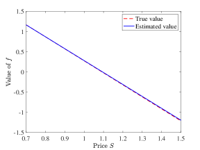
The CIR model
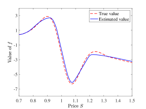
The GLV model
In Figure 1, we compare the learned optimal policy function obtained by our method (blue solid line) with the theoretically optimal policy function (red dashed line). The left figure is with the CIR model, while the right is with the GLV model. It can be observed that our algorithm can capture the optimal policy function quite well.
The CIR model
The GLV model
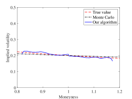
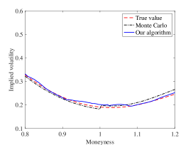
Next we compare the learned option pricing functions obtained by our algorithm and the benchmark pricing functions obtained by the finite difference method for the PDE model with true parameters. To measure their difference, we transform the price functions into the implied volatility functions against the moneyness (the ratio of spot price to strike price). In particular, we focus on out-of-money options, plotting the implied volatility curves against the moneyness for call options when the moneyness is less 1, and for put options when the moneyness is greater than 1. In Figure 2, we present the benchmark implied volatility curve (red dashed line) and the learned implied volatility curve (blue solid line), indicating that our method performs very well. It is worth pointing out that our method is less accurate for deep out-of-money options. The reasoning is the following. Our method outputs a price function, which is very close to the true solution. However, implied volatility is very sensitive to errors when option prices are lower.
Further, we investigate whether the errors in estimating the optimal policy function significantly affect the accuracy of option pricing. To do this, we assume is known, and for a given , we generate random stock paths according to the real-world stock price process (18). For each path, we can obtain through the learned optimal policy function . Then we can employ the Monte-Carlo simulation to estimate the expectation as given in (4). Repeating the above procedure for different initial stock prices leads to an option price function. In Figure 2, we plot the corresponding implied volatility curves using the black dash-dotted line. It can be observed that the black dash-dotted curves are close to the other two curves, implying that the estimation errors for the optimal policy function have a negligible impact on the accuracy of our pricing methodology.
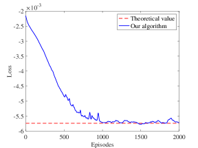
The CIR model
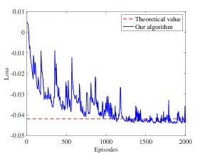
The GLV model
Lastly, we investigate the convergence of our algorithms against the number of episodes. For illustration, we consider the case for learning the optimal policy function. We take additional 25,600 sample paths as the validation dataset. For each episode in the training procedure, we also compute the loss function over the validation dataset, which we call the loss curve. In Figure 3, we plot the loss curve (the blue solid line) against the number of episodes for the CIR model (left panel) and GLV model (right panel), respectively. For comparison, we also plot the theoretical value (the red dashed line) that the loss curve converges to.111111The theoretical value is nothing but the negative value function associated with the portfolio optimization problem. Notably, after approximately 1,000 episodes, the loss curve converges towards the theoretical value.
5 Future Research Directions
For potential future research directions along this line, we may enhance the deep learning algorithm used in our approach so that the amount of data required is close to reality. Besides, it is worth extending our pricing methodology to an incomplete market where infinitely many pricing kernels exist.
Appendix A Appendix
Proof of Theorem 2.1.
It is easy to see that the optimal terminal wealth for problem (6) is the optimal solution for
| (19) |
The optimal terminal wealth is . Hence the wealth process is. Since with satisfying we have
which means . Notice that is a feedback policy and observable with respect to . \Halmos
Proof of Proposition 3.1.
According to Theorem 2.1, for each , is the unique maximizer of and is independent of . It is clear that also maximizes .
Suppose has another maximizer , then for any . Hence we have
Hence we have for almost all , which contradicts the fact that is the unique maximizer of . \Halmos
References
- Black and Scholes (1973) Black F, Scholes M (1973) The pricing of options and corporate liabilities. Journal of Political Economy 81(3):637–654.
- Bouchouev and Isakov (1997) Bouchouev I, Isakov V (1997) The inverse problem of option pricing. Inverse Problems 13(5):L11.
- Buehler et al. (2019) Buehler H, Gonon L, Teichmann J, Wood B (2019) Deep hedging. Quantitative Finance 19(8):1271–1291.
- Cox et al. (1985) Cox JC, Ingersoll JE, Ross SA (1985) A theory of the term structure of interest rates. Econometrica 53(2):385–407.
- Dai et al. (2023) Dai M, Dong Y, Jia Y (2023) Learning equilibrium mean-variance strategy. Mathematical Finance 33(4):1166–1212.
- Dupire (1994) Dupire B (1994) Pricing with a smile. Risk 7(1):18–20.
- Guo et al. (2020) Guo X, Xu R, Zariphopoulou T (2020) Entropy regularization for mean field games with learning. Math. Oper. Res. 47(4):3239–3260.
- Hambly et al. (2021) Hambly BM, Xu R, Yang H (2021) Recent advances in reinforcement learning in finance. Mathematical Finance 33(3):437–503.
- Heston (1993) Heston SL (1993) A closed-form solution for options with stochastic volatility with applications to bond and currency options. Review of Financial Studies 6(2):327–343.
- Hull and White (1987) Hull J, White A (1987) The pricing of options on assets with stochastic volatilities. The Journal of Finance 42(2):281–300.
- Hull (2014) Hull JC (2014) Options, Futures, and other Derivatives (Prentice Hall: Pearson), 9 edition.
- Jia and Zhou (2022) Jia Y, Zhou XY (2022) Policy evaluation and temporal-difference learning in continuous time and space: A martingale approach. Journal of Machine Learning Research 23(1):6918–6972.
- Jiang et al. (2003) Jiang L, Chen Q, Wang L, Zhang J (2003) A new well-posed algorithm to recover implied local volatility. Quantitative Finance 3(6):451–457.
- Kingma and Ba (2014) Kingma D, Ba J (2014) Adam: A method for stochastic optimization. International Conference on Learning Representations .
- Kou (2002) Kou SG (2002) A jump-diffusion model for option pricing. Management Science 48(8):1086–1101.
- Merton (1976) Merton RC (1976) Option pricing when underlying stock returns are discontinuous. Journal of Financial Economics 3(1):125–144.
- Wang et al. (2020) Wang H, Zariphopoulou T, Zhou X (2020) Exploration versus exploitation in reinforcement learning: a stochastic control approach. Journal of Machine Learning Research 21:1–34.
- Wang and Zhou (2020) Wang H, Zhou XY (2020) Continuous-time mean–variance portfolio selection: A reinforcement learning framework. Mathematical Finance 30(4):1273–1308.