Asymptotic Normality of the Conditional Value-at-Risk based Pickands Estimator

Abstract

The Pickands estimator for the extreme value index is beneficial due to its universal consistency, location, and scale invariance, which sets it apart from other types of estimators. However, similar to many extreme value index estimators, it is marked by poor asymptotic efficiency. Chen (2021) introduces a Conditional Value-at-Risk (CVaR)-based Pickands estimator, establishes its consistency, and demonstrates through simulations that this estimator significantly reduces mean squared error while preserving its location and scale invariance. The initial focus of this paper is on demonstrating the weak convergence of the empirical CVaR in functional space. Subsequently, based on the established weak convergence, the paper presents the asymptotic normality of the CVaR-based Pickands estimator. It further supports these theoretical findings with empirical evidence obtained through simulation studies.

Keywords: Pickands estimator; Extreme value index; Conditional Value-at-Risk; Asymptotic normality; Second-order regular variation

1 Introduction

Suppose $X$ is a random variable (r.v.) with a distribution function (d.f.) $F$, and $X_{1},X_{2},\ldots,X_{n}$ is the sequence of independent samples of $X$. The extreme value d.f. with shape parameter $\gamma\in\mathbb{R}$ (shift parameter $0$ and scale parameter $1$) is defined by

$$G_{\gamma}(x)=\begin{cases}\exp\left\{-(1+\gamma x)^{-1/\gamma}\right\},&\quad\text{for }\gamma\neq 0,\ 1+\gamma x>0,\\ \exp\left\{-e^{-x}\right\},&\quad\text{for }\gamma=0,\ x\in\mathbb{R}.\end{cases}$$

The d.f. $F$ belongs to the domain of attraction of $G_{\gamma}$ for some $\gamma\in\mathbb{R}$, noted as $F\in\mathscr{D}(G_{\gamma})$, if there exists a sequence of constants $a_{n}>0$ and $b_{n}\in\mathbb{R}$ such that

$$\lim_{n\rightarrow\infty}P\left\{\max\left(X_{1},\ldots,X_{n}\right)\leqslant a_{n}x+b_{n}\right\}=\lim_{n\rightarrow\infty}F^{n}\left(a_{n}x+b_{n}\right)=G_{\gamma}(x).$$ (1.1)

This $\gamma$ is called the extreme value index of $F$.

An alternative characterization of $\gamma$ in extreme value theory can be provided using the generalized Pareto distribution (GPD), which has d.f.

$$H_{\gamma}(x)=\begin{cases}1-(1+\gamma x)^{-1/\gamma},&\quad\text{for }\gamma\neq 0,\ x\geq 0,\ 1+\gamma x>0,\\ 1-e^{-x},&\quad\text{for }\gamma=0,\ x\geq 0.\end{cases}$$

Note that $H_{\gamma}$ with $\gamma>0$ yields a Pareto distribution; $H_{0}$ coincides with the exponential distribution. Additionally, $H_{\gamma}$ with $\gamma<0$ exhibits a finite right endpoint, particularly with $\gamma=-1$ resulting in a uniform distribution on the interval $(0,1)$.

Let $x_{+}=\sup\{x\in\mathbb{R}:F(x)<1\}$ denote the right endpoint of a d.f. $F$. For $u\in\mathbb{R}$ such that $F(u)<1$, let the excess d.f. denoted by $F_{u}(x)=P(X-u\leq x|X>u)$ for $x\geq 0$. The fundamental result of Pickands (1975) is that $F\in\mathscr{D}(G_{\gamma})$ if and only if for $u<x_{+}$ there exists a positive, measurable function $\sigma(u)$, such that

$$\lim_{u\to x_{+}}F_{u}(\sigma(u)x)=H_{\gamma}(x),\quad\text{for }x\geq 0.$$ (1.2)

Formula (1.2) suggests modeling the unknown excess d.f. $F_{u}$ in the case of $F\in\mathscr{D}(G_{\gamma})$ by the parametric family $H_{\gamma}(\cdot/\sigma)$, where $\gamma\in\mathbb{R}$ and $\sigma>0$. Consequently, the upper tail of $F$ can be approximated by that of a GPD.

Hence, understanding the extreme value index $\gamma$ is crucial for modeling maxima and estimating extreme quantiles. The estimation of $\gamma$, besides high quantile estimation, is one of the most crucial problem in univariate extreme value theory.

Let $X_{1}^{(n)},X_{2}^{(n)},\cdots,X_{n}^{(n)}$ denote the descending order statistics of $X_{1},\ldots,X_{n}$. Pickands (1975) proposed a simple estimator for $\gamma$, constructed in terms of log-spacings of order statistics:

$$\widehat{\gamma}_{n}^{P}(m):=\frac{1}{\log 2}\log\left(\frac{X_{m}^{(n)}-X_{2m}^{(n)}}{X_{2m}^{(n)}-X_{4m}^{(n)}}\right),\quad\text{for }m=1,\ldots,\lfloor n/4\rfloor,$$

where $\lfloor x\rfloor$ is the floor of a real number $x$. Compared with the Hill (1975) estimator and the probability weighted moment estimator proposed by Hosking et al. (1985), the primary benefits of the Pickands estimator include the invariant property under location and scale shift, and the consistency for any $\gamma\in\mathbb{R}$ under intermediate sequence such that $m_{n}\to\infty$, $m_{n}/n\to 0$ as $n\to\infty$.

However, the Pickands estimator exhibits relatively poor asymptotic variance. To address the drawback, Yun (2002) first generalized the Pickands estimator by

$$\widehat{\gamma}_{n,m}^{Y}(u,v):=\frac{1}{\log v}\log\frac{X_{m}^{(n)}-X_{[um]}^{(n)}}{X_{[vm]}^{(n)}-X_{[uvm]}^{(n)}},\quad u,v>0,u,v\neq 1,$$ (1.3)

where $1\leqslant m,[um],[vm],[uvm]\leqslant n$ and $[x]$ denotes the integer part of $x\in\mathbb{R}$. The estimator is constructed by the linear combinations of the logarithm of the spacing between intermediate order statistics. The spacings are generalized and determined by $u$ and $v$. The optimal $(u^{\ast},v^{\ast})$ with $0<v\leq u<1$ along $\gamma$ which minimizes the asymptotic variance is approximated numerically. Then, the estimation is conducted in an adaptive manner.

All these previously mentioned estimators are constructed in terms of quantities of order statistics (or empirical quantiles of the d.f.). Alternatively, a new quantity named Conditional Value at Risk (CVaR) order statistic (or empirical super-quantile) can be introduced in extreme value index estimators. Chen (2021) defined the empirical descending CVaR order statistics $Y_{1}^{(n)}\geqslant Y_{2}^{(n)}\geqslant\cdots\geqslant Y_{n}^{(n)}$ by

$$Y_{k}^{(n)}:=\frac{1}{k}\sum_{i=1}^{k}X_{i}^{(n)},\quad k=1,\ldots,n,$$ (1.4)

where $X_{i}^{(n)}$ are the descending order statistics, as in the definition of the original Yun (2002) estimator in (1.3). This $\{Y_{k}^{(n)}\}_{k=1}^{n}$ are named CVaR order statistics, and its equivalence to the empirical CVaR, i.e.,

$$Y_{k}^{(n)}=\widehat{\mathrm{CVaR}}_{1-\frac{k}{n}}\quad k=1,\ldots,n.$$

was also explained. For further relation to the CVaR and CVaR estimation we refer to Rockafellar and Uryasev (2002), Acerbi and Tasche (2002), John Manistre and Hancock (2005), Brazauskas et al. (2008), Gao and Wang (2011), etc. Chen (2021) incorporated CVaR order statistics into the framework by Yun (2002) to introduce the CVaR-based Pickands estimator by

$$\widehat{\gamma}_{n,m}(u,v):=\frac{1}{\log v}\log\frac{Y_{m}^{(n)}-Y_{[um]}^{(n)}}{Y_{[vm]}^{(n)}-Y_{[uvm]}^{(n)}},\quad u,v>0,u,v\neq 1,$$ (1.5)

where $1\leqslant m,[um],[vm],[uvm]\leqslant n$ and $[x]$ denotes the integer part of $x\in\mathbb{R}$. He showed the consistency of the estimator within $\gamma<1$. The CVaR can be viewed as an equal-weighted average of Value-at-Risk (VaR) (Rockafellar and Uryasev, 2002). Therefore, with $\gamma$ not too large, i.e., the distribution tail is not too heavy, the idea of equal-weighted averaging can reduce the variance of the estimator for the extreme value index (see Sections 4 and 5).

The rest of the paper is organized as follows. In Section 2, we introduce the CVaR-based regular variation condition in extreme value theory. Section 3 focuses on the weak convergence of empirical CVaR in functional space. Section 4 exhibits the asymptotic normality result of the CVaR-based Pickands estimator. Section 5 provides simulation studies supporting the asymptotic normality result, while Section 6 presents the conclusions.

2 The CVaR-based Regular Variation Conditions

2.1 First-order Conditions

A sequence of positive integers $m=m(n)$ is called an intermediate sequence if $m\to\infty$ and $m/n\to 0$ as $n\to\infty$. Define $U(x):=F^{-1}(1-1/x)$, where $F^{-1}$ denotes the quantile function of $F$. Then the condition $F\in\mathscr{D}(G_{\gamma})$ is equivalent to the existence of a positive, measurable function $a(x)$ defined on a neighborhood of infinity such that

$$\lim_{t\to\infty}\frac{U(\frac{t}{y})-U(t)}{a(t)}=\frac{y^{-\gamma}-1}{\gamma}:=h_{\gamma}(y),\quad y>0$$ (2.1)

where $h_{\gamma}(y)$ has to be read as $\log{\frac{1}{y}}$ in case $\gamma=0$. Moreover, (1.1) holds with $b_{n}:=U(n)$ and $a_{n}:=a(n)$. See (De Haan, 1984, Lemma 1), (De Haan and Ferreira, 2006, Theorem 1.1.6).

Remark 2.1.

The auxiliary function $a$ in (2.1) necessarily satisfies

$$\lim_{t\to\infty}\frac{a(\frac{t}{y})}{a(t)}=y^{-\gamma},\quad y>0$$ (2.2)

that is, $a$ is regularly varying with index $\gamma$, denoted as $a\in RV_{\gamma}$. If $a\in RV_{0}$, $a$ is called a slowly varying function. Both (2.1) and (2.2) hold locally uniformly in $0<y<\infty$ (Bingham et al., 1989, Thereom $1.5.2$).

Suppose $F$ has a finite mean and define

$$V(x):=\frac{1}{x}\int_{0}^{x}F^{-1}(1-s)ds=\frac{1}{x}\int_{0}^{x}U(\frac{1}{s})ds.$$ (2.3)

Chen (2021) showed that if $F\in\mathscr{D}(G_{\gamma})$, there exists a positive, measurable function $a(t)$ defined on a neighborhood of infinity such that

$$\lim_{t\to\infty}\frac{V(\frac{y}{t})-V(\frac{1}{t})}{a(t)}=\frac{1}{y}\int_{0}^{y}h_{\gamma}(w)dw-\int_{0}^{1}h_{\gamma}(w)dw:=\tilde{h}_{\gamma}(y)\quad\text{ for }y>0,$$ (2.4)

alternatively, for $y>0$,

$$\frac{V(\frac{y}{t})-V(\frac{1}{t})}{a(t)}=\tilde{h}_{\gamma}(y)+\tilde{R}(t,y),\quad\tilde{R}(t,y)=o(1)\>\text{as }t\to\infty,$$ (2.4’)

where $\tilde{h}_{\gamma}(y)=\frac{y^{-\gamma}-1}{\gamma(1-\gamma)}$ for $\gamma<1$ and $\tilde{h}_{\gamma}(y)=-log(y)$ in case $\gamma=0$. He proved the consistency of the CVaR-based Pickands estimator, $\widehat{\gamma}_{n,m}(u,v)$, under the condition $F\in\mathscr{D}\left(G_{\gamma}\right)$ of (2.1) for the intermediate sequences $m=m(n)$ as $n\to\infty$.

2.2 Second-order Conditions

Condition 2.1.

For some $x_{0}>1$ the tail quantile function $U$ is absolutely continuous on $[x_{0},\infty)$ with density $u$. There are $\gamma\in\mathbb{R},\ \rho\leq 0,d\in\mathbb{R}$, and $A\in RV_{\rho}$ with $\lim_{t\to\infty}A(t)=0$ such that, denoting $a(t)=tu(t)$, we have

$$\lim_{t\to\infty}\frac{\log a(\frac{x}{y})-\log a(x)-\gamma\log\frac{1}{y}}{A(t)}=dh_{\rho}(y),\quad\text{for }y>0,$$ (2.5)

and $a(x)$ is regularly varying with index $\gamma$.

Remark 2.2.

Condition 2.1 actually imposes a rate of convergence in (2.1). Define

$$h(y;x)=\frac{U(\frac{x}{y})-U(x)}{a(x)}\quad\text{for }y>0,\ x\geq x_{0},$$ (2.6)

$$H_{\gamma,\rho}(y)=\int_{y}^{1}w^{1-\gamma}h_{\rho}(w)dw=\frac{1}{\rho}\biggl{(}\frac{y^{-(\rho+\gamma)}-1}{\rho+\gamma}-\frac{y^{-\gamma}-1}{\gamma}\biggr{)},\quad\text{for }y>0,$$ (2.7)

with the appropriate limits in case $\gamma=0,\ \rho=0$, or $\gamma+\rho=0$. Condition 2.1 now implies

$$\lim_{t\to\infty}\frac{h(y;t)-h_{\gamma}(y)}{A(t)}=dH_{\gamma,\rho}(y)$$ (2.8)

The latter is consistent with the framework of second-order generalized variation (De Haan and Stadtmüller, 1996) and is introduced in Pereira (1994) and Drees (1995).

Condition 2.2.

Let $A$ and $d$ be as in condition 2.1. The intermediate sequence $m=m(n)$ satisfies

• case $d\neq 0$: $\lim_{n\to\infty}\sqrt{m}A(\frac{n}{m})$ exists;

• case $d=0$: $\sup_{n\geq 2}\sqrt{m}A(\frac{n}{m})<\infty$.

In both cases, we denote $r:=\lim_{n\to\infty}d\sqrt{m}A(\frac{n}{m})$.

To derive the asymptotic bias of the CVaR-based estimator, one needs to consider the second-order behavior of $V$. The second-order regular variation limit function for $V$ will be similar. Define that

$$\tilde{h}_{(}y;x):=\frac{1}{y}\int_{0}^{y}h(w;x)dw-\int_{0}^{1}h(w;x)dw=\frac{V(\frac{y}{x})-V(\frac{1}{x})}{a(x)}.$$ (2.9)

Then, the second-order behavior of $V$ is demonstrated in the following corollary.

Corollary 2.1.

If Condition 2.1 holds with $\gamma<1$ and $V(\frac{y}{t})=\frac{1}{y}\int_{0}^{y}U(\frac{t}{s})$,

$$\lim_{t\to\infty}\frac{\tilde{h}_{(}y;t)-\tilde{h}_{\gamma}(y)}{A(t)}=d\tilde{H}_{\gamma,\rho}(y),\quad y>0,$$ (2.10)

where

$$\tilde{H}_{\gamma,\rho}(y):=\frac{1}{y}\int_{0}^{y}H_{\gamma,\rho}(x)dx-\int_{0}^{1}H_{\gamma,\rho}(x)dx.$$ (2.11)

3 The Empirical CVaR Process

Remark 3.1.

Let $X$ be a random variable with d.f. $F$ where $F\in\mathscr{D}(G_{\gamma})$, and let $k$ be an integer with $0<k<1/\gamma_{+}$, where $\gamma_{+}:=\max(0,\gamma)$. Then, $E(|X|^{k})$ is finite. In particular, if $\gamma<1$, $E|X|$ is finite; if $\gamma<\frac{1}{2}$, $E(X^{2})$ is finite and thus, the variance of random variable $X$ exists (De Haan and Ferreira, 2006, Theorem 5.3.1).

This implies that the CVaR-based estimators are valid for $\gamma<\frac{1}{2}$, contingent upon the finite variance of the random variable with distribution function $F$, where $F\in\mathscr{D}(G_{\gamma})$, and, of course, the existence of CVaR ($\gamma<1$).

The stochastic process with the empirical VaR process is defined by

$$B_{n}(t):=\sqrt{m}\frac{X_{[mt]}^{(n)}-U(\frac{n}{mt})}{a(\frac{n}{m})},\quad 0<t\leq\frac{n}{m}.$$

Assume that Condition 2.1 and 2.2 hold, from Proposition 1 of Resnick and Staăricaă (1999), the stochastic process

$$B_{n}(t):=\sqrt{m}\frac{X_{[mt]}^{(n)}-U(\frac{n}{mt})}{a(\frac{n}{m})}\Rightarrow B(t)$$ (3.1)

in $D(0,\infty)$ as $n\to\infty,m\to\infty$ and $m/n\to 0$, where $B(t)=t^{-\gamma-1}W(t)$ and $W$ is a standard Brownian motion.

Theorem 3.1.

Suppose $F\in\mathscr{D}(G_{\gamma})$ with $\gamma<\frac{1}{2}$, and Conditions 2.1 and 2.2 hold, and define the stochastic process with empirical CVaR process by

$$\tilde{B}_{n}(t):=\sqrt{m}\dfrac{Y_{[mt]}^{(n)}-V(\dfrac{mt}{n})}{a(\dfrac{n}{m})},\quad 0<t\leq\frac{n}{m}.$$

Then,

$$\tilde{B}_{n}(t)\Rightarrow\tilde{B}(t)$$ (3.2)

in $D(0,\infty)$, where

$$\tilde{B}(t) =\frac{1}{t}\int_{0}^{t}s^{-\gamma-1}W(s)ds,\quad t>0.$$

Observe that when $\gamma<\frac{1}{2}$, the stochastic process $\tilde{B}(t),\ t>0$ is mean-zero normally distributed with the finite variance

$$Var(\tilde{B}(t))=\begin{cases}\frac{2}{(1-\gamma)(1-2\gamma)}t^{-2\gamma-1},\quad\gamma\neq 0\ \&\ \gamma<\frac{1}{2},\\ \frac{2}{t},\quad\gamma=0.\end{cases}$$ (3.3)

Note that the weak convergence of the empirical CVaR holds in (3.2) requires a finite variance of $\tilde{B}(t)$, implying $\gamma<\frac{1}{2}$. This aligns with the consistency that the CVaR-based estimators are valid when $\gamma<\frac{1}{2}$ as indicated in Remark 3.1. Besides, with $t_{1},t_{2}>0$,

$$Cov(\tilde{B}(t_{1}),\tilde{B}(t_{2})) :=\sigma(t_{1},t_{2})$$

$$=\begin{cases}(t_{1}t_{2})^{-1}\left[h_{1}(\gamma)(t_{1}\land t_{2})^{1-2\gamma}-h_{2}(\gamma)(t_{1}\land t_{2})^{1-\gamma}(t_{1}\lor t_{2})^{-\gamma}\right],\quad\gamma\neq 0\;\&\;\gamma<\frac{1}{2}\\ \\ (t_{1}\lor t_{2})^{-1}\left[2-\log{(t_{1}\land t_{2})}+\log{(t_{1}\lor t_{2})}\right],\quad\gamma=0,\end{cases}$$

where $h_{1}(\gamma)=\frac{1}{\gamma(1-\gamma)(1-2\gamma)}$ and $h_{2}(\gamma)=\frac{1}{\gamma(1-\gamma)}$.

4 Asymptotic Normality of the CVaR-based Pickands Estimator

Standing on Theorem 3.1 in Section 3, we can derive the following theorem on the asymptotic normality of the CVaR-based Pickands estimator.

Theorem 4.1 (Asymptotic Normality).

Suppose $F\in\mathscr{D}(G_{\gamma})$ with $\gamma<\frac{1}{2}$, and Conditions 2.1 and 2.2 hold. Let $u,v>0$ with $u,v\neq 1$ and define the function

$$g(v,uv)=\begin{cases}\frac{v^{-\gamma}-(uv)^{-\gamma}}{\gamma(1-\gamma)},\quad\gamma\neq 0\\ \log{u},\quad\gamma=0.\end{cases}$$

Then,

$$\sqrt{m}(\widehat{\gamma}_{n,m}(u,v)-\gamma)\xrightarrow{d}\mathcal{N}\left(\frac{r\cdot b(u,v,\gamma,\rho)}{v^{\gamma}\log{v}},\frac{\sigma_{\gamma}^{2}(u,v)}{v^{2\gamma}\log^{2}{v}}\times\frac{1}{g^{2}(v,uv)}\right)\quad\text{as}\ n\to\infty,\qquad$$

where

$$b(u,v,\gamma,\rho)=\frac{\tilde{H}_{\gamma,\rho}(uv)-\tilde{H}_{\gamma,\rho}(v)-v^{-\gamma}\tilde{H}_{\gamma,\rho}(u)}{v^{-2\gamma}}\frac{\gamma(1-\gamma)}{1-u^{-\gamma}},$$

$$\sigma_{\gamma}^{2}(u,v) =\begin{cases}\frac{2}{(1-\gamma)(1-2\gamma)}(1+v^{-1})(1+u^{-2\gamma-1})+\mathscr{G}(u,v),\quad\gamma\neq 0\\ (1+u^{-1})(1+v^{-1})+\mathscr{G}(u,v),\quad\gamma=0,\end{cases}$$

and

$$\mathscr{G}(u,v)=2\left(-\sigma(1,u)-v^{\gamma}\sigma(1,v)+v^{\gamma}\sigma(1,uv)+v^{\gamma}\sigma(u,v)-v^{\gamma}\sigma(u,uv)+v^{2\gamma}\sigma(v,uv)\right).$$

5 Simulations

In the simulation study, two estimators are included: the estimator $\widehat{\gamma}_{n,m}^{Y}(u,v)$ in (1.3) by Yun (2002) and the CVaR-based Pickands estimator $\widehat{\gamma}_{n,m}(u,v)$ in (1.5). The parameters $u$ and $v$ are set to $u=v=2$, rendering the first estimator equivalent to the Pickands estimator introduced by Pickands (1975). The distributions involved in the experiment include Generalized Extreme Value and Generalized Pareto distributions, as they are applicable for $\gamma\in\mathbb{R}$. We compare two ratios for the two estimators. The first is the ratio of asymptotic variances, and the second is the ratio of estimated variances through simulation. For details on the asymptotic variance of the estimator $\widehat{\gamma}_{n,m}^{Y}(u,v)$, please refer to Yun (2002).

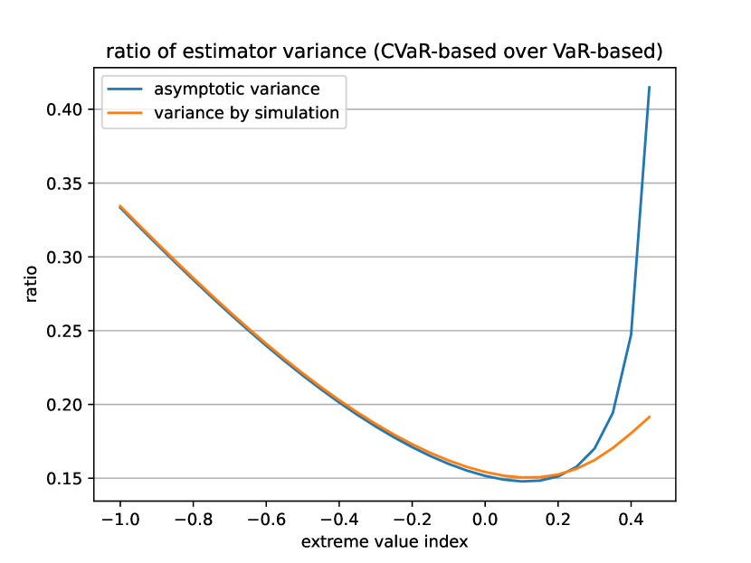
Figure 1: Generalized Extreme Value distribution.

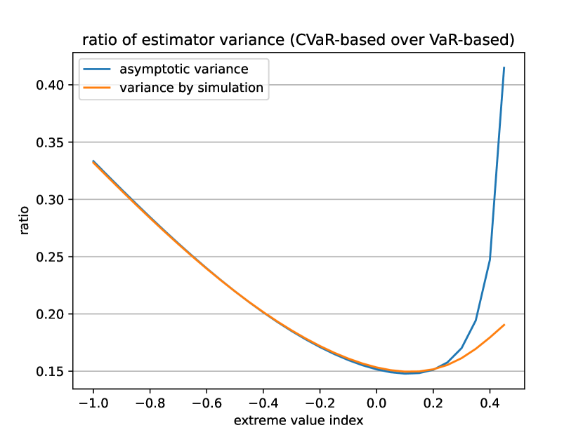
Figure 2: Generalized Pareto distribution.

The results presented in Figures 2 and 2 are obtained from $10^{4}$ samples with intermediate order statistics size $m=10^{2}$ and sample size $n=10^{4}$. Each distribution is sampled from the same set of random seeds. The two figures depict the ratio of asymptotic variance and the ratio of estimated variance by simulation across the range $-1\leq\gamma<0.5$. It can be observed that the two ratios coincide within the range of $\gamma=-1$ to around $0.2$. Their discrepancies emerge and increase as $\gamma$ approaches $0.5$. This is because as $\gamma$ approaches $0.5$, the CVaR-based Pickands estimator eventually exhibits an infinite asymptotic variance. On the other hand, the estimated variance by simulation continues to increase but never reaches infinity. When focusing on the ratio of asymptotic variance, we can also observe that the CVaR-based Pickands estimator substantially reduces the asymptotic variance to approximately $0.15$ to $0.45$ times that of the original Pickands estimator.

6 Conclusion

This paper studies the asymptotic behavior of the CVaR-based Pickands estimator proposed by Chen (2021). The CVaR-based second-order regular variation condition is derived. Then, the weak convergence of empirical CVaR in functional space is established under the derived second-order condition. Subsequently, the asymptotic normality of the estimator is presented, standing on the result of weak convergence of empirical CVaR, and is empirically validated through simulation.

Appendix A Proofs

Proof of Corollary 2.1

Proof.

When $\gamma<1$ and $\gamma\neq 0$, since $F$ has a finite mean, both the left hand side and the right hand side in (2.8) are integrable functions. By Dominated Convergence Theorem, the integration is preserved by convergence. We can take integral from 0 to $y$ both left and right hand sides and take subtraction with $y=1$ to get (2.10). ∎

Proof of Theorem 3.1

Proof.

First note that $X_{mt}^{(n)}\stackrel{{\scriptstyle d}}{{=}}F_{n}^{-1}(1-\frac{mt}{n})$ and $Y_{mt}^{(n)}\stackrel{{\scriptstyle d}}{{=}}\frac{1}{t}\int_{0}^{t}F_{n}^{-1}(1-\frac{ms}{n})ds$ where $F_{n}^{-1}$ is the empirical quantile function for the random variable $X$. Thus, $\tilde{B}_{n}(t)=\frac{1}{t}\int_{0}^{t}B_{n}(s)ds$.

The uniform convergence of the process $B_{n}(t)$ allows us to take integral both at the LHS and RHS in (3.1), so we can get (3.2) and (3.3). When $\gamma\neq 0$, $Var(\tilde{B}(t))=t^{-2}\int_{0}^{t}(s^{-\gamma}-t^{-\gamma})^{2}ds$ and the convergence of the integral requires $\gamma<\frac{1}{2}$. ∎

Proof of Theorem 4.1

Proof.

From Proposition 1, if $F\in\mathscr{D}(G_{\gamma})$ with $\gamma<\frac{1}{2}$, we have

$$\frac{Y_{[vm]}^{(n)}-Y_{[uvm]}^{(n)}}{a(\dfrac{n}{m})} =\frac{V(\frac{vm}{n})-V(\frac{uvm}{n})}{a(\dfrac{n}{m})}+\frac{1}{\sqrt{m}}(\tilde{B}_{n}(v)-\tilde{B}_{n}(uv))$$

$$=g(v,uv)+o_{p}(1)$$

since $\tilde{B}_{n}(v)-\tilde{B}_{n}(uv)$ has asymptotically a normal distribution. Thus, as we define $A_{n,m}(u,v)=\frac{Y_{m}^{(n)}-Y_{[um]}^{(n)}}{Y_{[vm]}^{(n)}-Y_{[uvm]}^{(n)}}$,

$$\sqrt{m}(A_{n,m}(u,v)-v^{\gamma}) =\sqrt{m}\frac{Y_{m}^{(n)}-Y_{[um]}^{(n)}-v^{\gamma}(Y_{[vm]}^{(n)}-Y_{[uvm]}^{(n)})}{Y_{[vm]}^{(n)}-Y_{[uvm]}^{(n)}}$$

$$\mathbin{\overset{p}{\kern 0.0pt\sim}}\frac{1}{g(v,uv)}\sqrt{m}\frac{Y_{m}^{(n)}-Y_{[um]}^{(n)}-v^{\gamma}(Y_{[vm]}^{(n)}-Y_{[uvm]}^{(n)})}{a(\dfrac{n}{m})}$$

$$=B_{n,m}(u,v)+C_{n,m}(u,v)\quad\text{as }n\to\infty,$$ (A.1)

where

$$B_{n,m}(u,v) :=\frac{1}{g(v,uv)}\{\tilde{B}_{n}(1)-\tilde{B}_{n}(u)-v^{\gamma}(\tilde{B}_{n}(v)-\tilde{B}_{n}(uv))\},$$

$$C_{n,m}(u,v) :=\frac{\sqrt{m}}{g(v,uv)}\frac{V(\frac{m}{n})-V(\frac{um}{n})-v^{\gamma}(V(\frac{vm}{n})-V(\frac{uvm}{n}))}{a(\frac{n}{m})}.$$

When $\gamma\neq 0$,

$$Var\left(\tilde{B}_{n}(1)-\tilde{B}_{n}(u)-v^{\gamma}(\tilde{B}_{n}(v)-\tilde{B}_{n}(uv))\right)$$

$$\quad=\begin{pmatrix}1&-1&-v^{\gamma}&v^{\gamma}\end{pmatrix}\begin{pmatrix}h(\gamma)&\sigma(1,u)&\sigma(1,v)&\sigma(1,uv)\\ \sigma(1,u)&u^{-2\gamma-1}h(\gamma)&\sigma(u,v)&\sigma(u,uv)\\ \sigma(1,v)&\sigma(u,v)&v^{-2\gamma-1}h(\gamma)&\sigma(v,uv)\\ \sigma(1,uv)&\sigma(u,uv)&\sigma(v,uv)&(uv)^{-2\gamma-1}h(\gamma)\end{pmatrix}\begin{pmatrix}1\\ -1\\ -v^{\gamma}\\ v^{\gamma}\end{pmatrix}$$

$$\quad=h(\gamma)(1+v^{-1})(1+u^{-2\gamma-1})+\mathscr{G}(u,v)$$

and when $\gamma=0$,

$$Var\left(\tilde{B}_{n}(1)-\tilde{B}_{n}(u)-v^{\gamma}(\tilde{B}_{n}(v)-\tilde{B}_{n}(uv))\right)$$

$$\quad=\begin{pmatrix}1&-1&-v^{\gamma}&v^{\gamma}\end{pmatrix}\begin{pmatrix}2&\sigma(1,u)&\sigma(1,v)&\sigma(1,uv)\\ \sigma(1,u)&\frac{2}{u}&\sigma(u,v)&\sigma(u,uv)\\ \sigma(1,v)&\sigma(u,v)&\frac{2}{v}&\sigma(v,uv)\\ \sigma(1,uv)&\sigma(u,uv)&\sigma(v,uv)&\frac{2}{uv}\end{pmatrix}\begin{pmatrix}1\\ -1\\ -v^{\gamma}\\ v^{\gamma}\end{pmatrix}$$

$$\quad=(1+u^{-1})(1+v^{-1})+\mathscr{G}(u,v)$$

Note here that

$$B_{n,m}(u,v) \xrightarrow{d}\frac{1}{g(v,uv)}\{B(1)-B(u)-v^{\gamma}(B(v)-B(uv)\}$$

$$\sim\mathcal{N}(0,\frac{\sigma_{\gamma}^{2}(u,v)}{g^{2}(v,uv)})\quad\text{as }n\to\infty.$$

Conditions (2.4’) and (2.10) imply that

$$C_{n,m}(u,v)=b(u,v,\gamma,\rho)\cdot d\sqrt{m}A(\frac{n}{m})+\sqrt{m}o(A(\frac{n}{m}))\quad\text{as }n\to\infty,$$ (A.2)

where

$$b(u,v,\gamma,\rho)=\frac{\tilde{H}_{\gamma,\rho}(uv)-\tilde{H}_{\gamma,\rho}(v)-v^{-\gamma}\tilde{H}_{\gamma,\rho}(u)}{v^{-2\gamma}}\frac{\gamma(1-\gamma)}{1-u^{-\gamma}}.$$

From the Condition 2.2, we know that $r:=\lim_{n\to\infty}d\sqrt{m}A(\frac{n}{m})$ is either $0$ or finite. Then $C_{n,m}(u,v)\to r\lambda$ as $n\to\infty$, and so from (A)

$$\sqrt{m}(A_{n,m}(u,v)-v^{\gamma})\xrightarrow{d}\mathcal{N}(rb(u,v,\gamma,\rho),\frac{\sigma_{\gamma}^{2}(u,v)}{g^{2}(v,uv)})\quad\text{as}\ n\to\infty.$$

Define the function $h(x):=\frac{1}{\log{v}}\log{x}$, Then, applying the Taylor expansion as $x\to v^{\gamma}$, we thus have

$$\sqrt{m}(\widehat{\gamma}_{n,m}(u,v)-\gamma) =\frac{\sqrt{m}}{v^{\gamma}\log{v}}(A_{n,m}(u,v)-v^{\gamma})+\sqrt{m}o_{p}(A_{n,m}(u,v)-v^{\gamma})$$

$$=\frac{\sqrt{m}}{v^{\gamma}\log{v}}(A_{n,m}(u,v)-v^{\gamma})+o_{p}(1)$$

$$\xrightarrow{d}\mathcal{N}\left(\frac{rb(u,v,\gamma,\rho)}{v^{\gamma}\log{v}},\frac{\sigma_{\gamma}^{2}(u,v)}{v^{2\gamma}\log^{2}{v}}\times\frac{1}{g^{2}(v,uv)}\right)\quad\text{as}\ n\to\infty.$$

∎

References

• Acerbi and Tasche (2002) C. Acerbi and D. Tasche. On the coherence of expected shortfall. Journal of Banking & Finance, 26(7):1487–1503, 2002.
• Bingham et al. (1989) N. H. Bingham, C. M. Goldie, J. L. Teugels, and J. Teugels. Regular Variation. Cambridge University Press, 1989.
• Brazauskas et al. (2008) V. Brazauskas, B. L. Jones, M. L. Puri, and R. Zitikis. Estimating conditional tail expectation with actuarial applications in view. Journal of Statistical Planning and Inference, 138(11):3590–3604, 2008.
• Chen (2021) T. Chen. Risk Management Approaches in Statistical Applications. PhD thesis, Stony Brook University, 2021.
• De Haan (1984) L. De Haan. Slow variation and characterization of domains of attraction. Statistical Extremes and Applications, 131:31–48, 1984.
• De Haan and Ferreira (2006) L. De Haan and A. Ferreira. Extreme value theory: an introduction, volume 21. Springer, 2006.
• De Haan and Stadtmüller (1996) L. De Haan and U. Stadtmüller. Generalized regular variation of second order. Journal of the Australian Mathematical Society, 61(3):381–395, 1996.
• Drees (1995) H. Drees. Refined pickands estimators of the extreme value index. The Annals of Statistics, 23(6):2059–2080, 1995.
• Gao and Wang (2011) F. Gao and S. Wang. Asymptotic behavior of the empirical conditional value-at-risk. Insurance: Mathematics and Economics, 49(3):345–352, 2011.
• Hill (1975) B. M. Hill. A simple general approach to inference about the tail of a distribution. The Annals of Statistics, 3(5):1163–1174, 1975.
• Hosking et al. (1985) J. R. M. Hosking, J. R. Wallis, and E. F. Wood. Estimation of the generalized extreme-value distribution by the method of probability-weighted moments. Technometrics, 27(3):251–261, 1985.
• John Manistre and Hancock (2005) B. John Manistre and G. H. Hancock. Variance of the cte estimator. North American Actuarial Journal, 9(2):129–156, 2005.
• Pereira (1994) T. T. Pereira. Second order behavior of domains of attraction and the bias of generalized pickands’ estimator. NIST Special Publication, pages 165–177, 1994.
• Pickands (1975) J. Pickands. Statistical inference using extreme order statistics. The Annals of Statistics, 3(1):119–131, 1975.
• Resnick and Staăricaă (1999) S. Resnick and C. Staăricaă. Smoothing the moment estimator of the extreme value parameter. Extremes, 1(3):263–293, 1999.
• Rockafellar and Uryasev (2002) R. T. Rockafellar and S. Uryasev. Conditional value-at-risk for general loss distributions. Journal of Banking & Finance, 26(7):1443–1471, 2002.
• Yun (2002) S. Yun. On a generalized pickands estimator of the extreme value index. Journal of Statistical Planning and Inference, 102(2):389–409, 2002.