Estimating the Hawkes process from a discretely observed sample path

Abstract

The Hawkes process is a widely used model in many areas, such as finance, seismology, neuroscience, epidemiology, and social sciences. Estimation of the Hawkes process from continuous observations of a sample path is relatively straightforward using either the maximum likelihood or other methods. However, estimating the parameters of a Hawkes process from observations of a sample path at discrete time points only is challenging due to the intractability of the likelihood with such data. In this work, we introduce a method to estimate the Hawkes process from a discretely observed sample path. The method takes advantage of a state-space representation of the incomplete data problem and use the sequential Monte Carlo (aka particle filtering) to approximate the likelihood function. As an estimator of the likelihood function the SMC approximation is unbiased, and therefore it can be used together with the Metropolis-Hastings algorithm to construct Markov Chains to approximate the likelihood distribution, or more generally, the posterior distribution of model parameters. The performance of the methodology is assessed using simulation experiments and compared with other recently published methods. The proposed estimator is found to have a smaller mean square error than the two benchmark estimators. The proposed method has the additional advantage that confidence intervals for the parameters are easily available. We apply the proposed estimator to the analysis of weekly count data on measles cases in Tokyo Japan and compare the results to those by one of the benchmark methods.

1 Introduction

In many applications that involve sequences of events such as earthquakes, infectious disease transmission in a community, and financial transactions, a frequently noted phenomenon is the temporal clustering of the events. A widely used statistical model for event sequences with this clustering feature is the Hawkes process (Hawkes,, 1971). Fitting the Hawkes process has most often been done by the maximum likelihood (ML) method (Ogata,, 1978; Ozaki,, 1979), which involves evaluating the logarithm of the likelihood of the model relative to a continuously observed sample path up to a censoring time and then maximising it as a function of the model parameters to be estimated. The Expectation-Maximisation (EM) algorithm has also been used to as a numerically more stable alternative to obtain the ML estimator of the Hakes process, especially in the multivariate case (Chornoboy et al.,, 1988).

When the sample path of the Hawkes process is not continuously monitored, or when the event times are recorded with limited precision, then the data available consists only of the values of the sample path at isolated observation time points or equivalently, counts of events in disjoint time intervals. However, the likelihood of the Hawkes process with such data is difficult to compute in general, so fitting the Hawkes process with such data is challenging. Recently, there have been attempts to address this challenge in the literature. Cheysson and Lang, (2022) proposed a spectral method, namely the maximum Whittle likelihood method, to estimate the Hawkes process with count data. They also established the consistency and asymptotic normality of the estimator. However, they did not provide an estimator for the standard errors of the estimator. Moreover, their method relies on the stationarity of the count time series and only works on data with regularly spaced observation time points and Hawkes process models with a constant background intensity.

Shlomovich et al., 2022b proposed a Monte Carlo Expectation-Maximization (MCEM) algorithm to estimate the parameters of the Hawkes process with count data, whereby the conditional expectation of the complete data loglikelihood in the Expectation- (E-) step of an EM cycle is approximated by a Monte Carlo (MC) method. They also applied the method to estimation of the multivariate Hawkes process from multi-type event count data (Shlomovich et al., 2022a, ). While their method does not require regularly spaced observation time points in the data or a constant background intensity in the Hawkes process model, due to their specific choice of the Monte Carlo sample generation method, the resulting MC estimate of the conditional expectation of the complete-data log-likelihood in the E-step is biased in general, and the bias seems to be inherited by the estimator of the model parameters. Also, they did not provided an estimator of the standard error of their model parameter estimator either.

Rizoiu et al., (2022) proposed a quasi-likelihood type method to estimate the Hawkes process from interval censored data or counts of events in different intervals. Their method works by defining the (quasi-) likelihood by pretending the Hawkes process is an inhomogeneous Poisson process with an intensity function equal to the mean intensity process of the Hawkes process and then maximising the thus defined likelihood as a function of the model parameters. Their method does not apply to stationary Hawkes processes since the corresponding Poisson process has only a single parameter, and so the corresponding quasi likelihood can not be used to distinguish different parameters of the Hawkes process. They did not address the question of standard error estimation either.

In this work we propose to approximate the ML estimator (MLE) of the parameters of the Hawkes process from a discretely observed sample path using Markov Chain Monte Carlo (MCMC). We first note that MLE is the maximum a posteriori (MAP) estimator with a flat prior for the parameter and therefore a posterior density proportional to the likelihood function. When the amount of data is large, by Laplace’s approximation (see e.g. van der Vaart,, 2007, $\S$10.2), the posterior distribution can typically be approximated by a Gaussian distribution with the mean equal to the ML/MAP estimator and the variance equal to the inverted negative Hessian matrix of the log-likelihood function. Therefore, we can approximate the MLE and the confidence intervals/regions using the posterior mean/median and the credible intervals/regions respectively. Even when the likelihood function is available analytically and easy to evaluate, finding the posterior mean/median and credible intervals analytically can still be difficult in practice and require numerical methods such as the Markov chain Monte Carlo (MCMC), which constructs an ergodic Markov chain with the desired posterior distribution as its stationary distribution by e.g. the Metropolis-Hastings algorithm (Metropolis et al.,, 1953; Hastings,, 1970) and then uses the occupation measure based on a sufficiently long run of it to approximate the posterior distribution.

In the context of estimating Hawkes process parameters from a discretely observed sample path, a further complication is that the likelihood function is not available analytically. However, we are able to construct an unbiased estimator of the intractable likelihood function, which allows us to use the Pseudo-Marginal Metropolis-Hastings (PMMH Andrieu and Roberts,, 2009) algorithm to construct a Markov chain with the correct stationary distribution. Our estimator of the likelihood is based on the sequential Monte Carlo (SMC), aka particle filtering method (Gordon et al.,, 1993; Kitagawa,, 1996). Therefore, our method might also be considered a special case of the particle marginal Metropolis-Hastings sampler of Andrieu et al., (2010), although they assumed a hidden Markov model where the hidden state evolves according to a Markov process and the observations of the state at different time points are conditionally independent, while in our case the hidden state process is not Markovian in general and the observations are not conditionally independent either. Although computationally intensive, our method is able to produce estimators that are statistically more efficient than the existing methods, and moreover, confidence intervals for the parameters are easily available.

The rest of the article is organized as follows. Section 2 presents the estimation problem and the proposed estimation method. Section 3 assesses the performance of the proposed SMC likelihood estimator and the approximate ML estimator on simulated data and compare performance with the spectral method of Cheysson and Lang, (2022) and the MCEM method of Shlomovich et al., 2022b . In Section 4 we analyse a weekly measles case count dataset from Tokyo Japan using the proposed method and compare the results with the previous analysis by Cheysson and Lang, (2022). Section 5 concludes with a discussion.

2 The data, the model, and the estimation method

Let $N(t),t\geq 0$ be the counting process corresponding to a Hawkes process, with $N(t)$ denoting the number of events of interest in the interval $(0,t]$. Suppose $N(t)$ is only observed at the the discrete time points, $0=t_{0}<t_{1}<t_{2}<\dots<t_{m}$. We assume that the observation time points are independent of the process $N(t)$, so they carries no information on the process and therefore can be treated as fixed in the inference. In addition to the observation times, the only data available is the values of process at the observation times, $N(t_{1}),\dotsc,N(t_{m})$. We shall use the convention $N(0)=0$, so the data is equivalent to the numbers of events in successive intervals $(t_{i-1},t_{i}]$, $n_{1}=N(t_{1}),\ n_{2}=N(t_{2})-N(t_{1}),\ \dotsc,\ n_{m}=N(t_{m})-N(t_{m-1})$.

Let the background event rate of the Hawkes process $N(t)$ be denoted by $\nu(t)$, and the excitation kernel function by $g(t)$, so that the intensity process of $N(t)$ relative to the natural filtration $\left\{\mathcal{F}_{t}\right\}_{t\geq 0}$, with $\mathcal{F}_{t}=\sigma\left\{N(s);\ s\leq t\right\}$, is given by

$$\lambda(t)=\nu(t)+\int_{0}^{t-}g(t-s)\,\mathrm{d}N(s)=\nu(t)+\sum_{i:\tau_{i}<t}g(t-\tau_{i}),$$ (1)

where $\tau_{1}<\tau_{2}<\dotsb$ denote the event times, so that $N(t)=\max\left\{i:\ \tau_{i}\leq t\right\}$. In the parametric inference problem to be considered in this work, the excitation kernel function is assumed to take some parametric form with parameters $\theta_{g}$, such as the exponential kernel $g(t;\theta_{g})=(\eta/\beta)e^{-t/\beta},\ t>0$ with parameters $\theta_{g}=(\eta,\beta)$ such that $0\leq\eta<1,\beta>0$, or the gamma kernel $g(t;\theta_{g})=\eta\Gamma(\alpha)^{-1}\beta^{-\alpha}t^{\alpha-1}e^{-t/\beta},\ t>0$, with parameters $\theta_{g}=(\eta,\alpha,\beta)$ such that $0\leq\eta<1$, $\alpha>0,\ \beta>0$. Note that, in these parametrisations, the integral of the kernel function is always $\eta$ and is assumed to be strictly less than 1, to ensure the asymptotic stationarity of the Hawkes process. The inference problem we consider is to assume a parametric form for $g$, and estimate the parameters of the model $\theta=(\theta_{\nu},\theta_{g})$ with a discretely observed sample path.

2.1 Likelihood of the model

The likelihood of the Hawkes process relative to a continuously observed sample path up to some censoring time $T$, $\left\{N(t),0\leq t\leq T\right\}$, or equivalently, the total number of events $N=N(0,T]$ up to time $T$ and the exact event times $\tau_{1},\dotsc,\tau_{N}$, is given explicitly by (Daley and Vere-Jones,, 2003)

$$L_{\mathrm{ful}}(\theta)=\left\{\prod_{i=1}^{N}\lambda(\tau_{i})\right\}\exp(-\int_{0}^{T}\lambda(t)\,\mathrm{d}t),$$

with $\lambda(t)$ given in (1) depending on the parameters $\theta$. The likelihood in this form can be exactly evaluated and numerically maximised as a function of $\theta$ to obtain the maximum likelihood estimator (MLE) of $\theta$.

With observations of the sample path at discrete time points only, the likelihood of the Hawkes model can be formally written as

$$L_{\mathrm{dis}}(\theta)=\Pr(N((t_{i-1},t_{i}])=n_{i},\ i=1,\dotsc,m).$$ (2)

However, there is no known explicit expressions for the likelihood function, so obtaining the MLE of the Hawkes process with discrete observations of the sample path only remains a challenge. In this work, we propose to obtain the MLE via sequential Monte Carlo (SMC) approximations to the likelihood functions.

2.2 Sequential Monte Carlo approximation to the likelihood

To present the SMC approximate of the likelihood $L_{\mathrm{dis}}(\theta)$ in (2), we first rewrite it in the following form

$$L_{\mathrm{dis}}(\theta) {}=\prod_{i=1}^{m}p_{\theta}(n_{i}|n_{1:i-1})$$ (3)

$${}=\prod_{i=1}^{m}\int p_{\theta}(n_{i}|n_{1:i-1},\tau_{1:N_{i}})P_{\theta}(\,\mathrm{d}\tau_{1:N_{i}}|n_{1:i-1}),$$ (4)

where $n_{1:i}$ is shorthand notation for $(n_{1},\dotsc,n_{i})$, $N_{i}=\sum_{j=1}^{i}n_{j}$, and $p_{\theta}(n_{i}|n_{1:i-1})$ is shorthand for $\Pr_{\theta}\left\{N((t_{i-1},t_{i}])=n_{i}|N((t_{i-2},t_{i-1}])=n_{i-1},\dotsc,N((t_{0},t_{1}])=n_{1})\right\}$. Similarly, $p_{\theta}(n_{i}|n_{1:i-1},\tau_{1:N_{i}})$ denotes the conditional probability of $N((t_{i-1},t_{i}])=n_{i}$ given the events $N((t_{i-2},t_{i-1}])=n_{i-1}$, $\dotsc$, $N((t_{0},t_{1}])=n_{1}$ and the times of all the first $N_{i}$ events, $\tau_{1:N_{i}}$, and $P_{\theta}(\,\mathrm{d}\tau_{1:N_{i}}|n_{1:i-1})$ denotes the conditional distribution of $\tau_{1:N_{i}}$ given the numbers of events in the first $i-1$ observation intervals. In the rest of this paper, we drop $\theta$ from the subscripts in various notations, while their dependence on $\theta$ is silently understood.

To approximate the integrals in (4) using Monte Carlo, we need to generate samples (aka particles) from the predictive distribution of the hidden event times $P(\,\mathrm{d}\tau_{1:N_{i}}|n_{1:i-1})$ and use the empirical distributions of the particles as an approximation of the predictive distribution, or from a suitable proposal distribution that dominates the predictive distribution and then use a weighted empirical distribution of the particles. Since we need to do this for all $i=1,\dotsc,m$, we do it in a sequential fashion by reusing the particles generated in the previous time step. That is, we use the sequential Monte Carlo method (Gordon et al.,, 1993; Kitagawa,, 1996).

Take an $\mathrm{i.i.d.}$ random sample (particles) $\tau_{1:N_{1},1}^{(j)},\ j=1\dotsc,J$ from a proposal distribution $Q(\,\mathrm{d}\tau_{1:N_{1}}|n_{1})$ that might depend on $n_{1}$. Then the associated importance sampling Monte Carlo (MC) approximation of the predictive distribution $P(\,\mathrm{d}\tau_{1:N_{1}})$ is given by

$$\widehat{P}(\,\mathrm{d}\tau_{1:N_{1}})=\frac{1}{J}\sum_{j=1}^{J}w_{1}^{(j)}\delta_{\tau_{1:N_{1},1}^{(j)}}(\,\mathrm{d}\tau_{1:N_{1}}),$$

with $\delta_{x}(\cdot)$ denoting the Dirac measure at $x$ and the importance weights $w_{1}^{(1:J)}$ given by the values of the Radon-Nikodym derivative of $P(\,\mathrm{d}\tau_{1:N_{1}})$ relative to $Q(\,\mathrm{d}\tau_{1:N_{1}}|n_{1})$ evaluated at the particles,

$$w_{1}^{(j)}=\bigg{[}\frac{P(\,\mathrm{d}\tau_{1:N_{1}})}{Q(\,\mathrm{d}\tau_{1:N_{1}}|n_{1})}\bigg{]}_{\tau_{1:N_{1}}=\tau_{1:N_{1},1}^{(j)}}.$$

So, the Monte Carlo approximation of $p(n_{1})=\int p(n_{1}|\tau_{1:N_{1}})P(\,\mathrm{d}\tau_{1:N_{1}})$ is given by

$$\widehat{p}(n_{1})=\int p(n_{1}|\tau_{1:N_{1}})\widehat{P}(\,\mathrm{d}\tau_{1:N_{1}})=\frac{1}{J}\sum_{j=1}^{J}w_{1}^{(j)}p(n_{1}|\tau_{1:N_{1},1}^{(j)}).$$

Suppose we have weighted particle approximations to the predictive distribution and the likelihood contribution respectively in the previous time step,

$$\widehat{P}(\,\mathrm{d}\tau_{1:N_{i-1}}|n_{1:i-2}) {}=\frac{1}{J}\sum_{j=1}^{J}w_{i-1}^{(j)}\delta_{\tau_{1:N_{i-1},i-1}^{(j)}}(\,\mathrm{d}\tau_{1:N_{i-1}}),$$

$$\widehat{p}(n_{i-1}|n_{1:i-2}) {}=\frac{1}{J}\sum_{j=1}^{J}w_{i-1}^{(j)}p(n_{i-1}|\tau_{1:N_{i-1},i-1}^{(j)},n_{1:i-2}).$$

Let $Q(\,\mathrm{d}\tau_{N_{i-1}+1:N_{i}}|n_{1:i},\tau_{1:N_{i-1}})$ be a proposal distribution for $\tau_{N_{i-1}+1:N_{i}}$ that dominates its conditional distribution $P(\,\mathrm{d}\tau_{N_{i-1}+1:N_{i}}|n_{1:i-1},\tau_{1:N_{i-1}})$. Note that similar to Pitt and Shephard, (1999), we allow the proposal distribution to depend on the observation in the $i$th interval, $n_{i}$. By the factorisation of the predictive distribution

$$P(\,\mathrm{d}\tau_{1:N_{i}}|n_{1:i-1}) =P(\,\mathrm{d}\tau_{1:N_{i-1}}|n_{1:i-1})P(\,\mathrm{d}\tau_{N_{i-1}+1:N_{i}}|n_{1:i-1},\tau_{1:N_{i-1}})$$ (5)

$$=\frac{p(n_{i-1}|\tau_{1:N_{i-1}},n_{1:i-2})}{p(n_{i-1}|n_{1:i-2})}P(\,\mathrm{d}\tau_{1:N_{i-1}}|n_{1:i-2})$$

$$\phantom{=}\times\left[\frac{P(\,\mathrm{d}\tau_{N_{i-1}+1:N_{i}}|n_{1:i-1},\tau_{1:N_{i-1}})}{Q(\,\mathrm{d}\tau_{N_{i-1}+1:N_{i}}|n_{1:i},\tau_{1:N_{i-1}})}\right]Q(\,\mathrm{d}\tau_{N_{i-1}+1:N_{i}}|n_{1:i},\tau_{1:N_{i-1}}),$$ (6)

we can first sample $\tau_{1:N_{i-1},i}^{(1:J)}$ from the plug-in estimate of the filtering distribution in the previous time step

$$\widehat{P}(\,\mathrm{d}\tau_{1:N_{i-1}}|n_{1:i-1}) =\frac{p(n_{i-1}|\tau_{1:N_{i-1}},n_{1:i-2})}{\widehat{p}(n_{i-1}|n_{1:i-2})}\widehat{P}(\,\mathrm{d}\tau_{1:N_{i-1}}|n_{1:i-2})$$

$$=\frac{\frac{1}{J}\sum_{j=1}^{J}p(n_{i-1}|\tau_{1:N_{i-1},i-1}^{(j)},n_{1:i-2})w_{i-1}^{(j)}\delta_{\tau_{1:N_{i-1},i-1}^{(j)}}(\,\mathrm{d}\tau_{1:N_{i-1}})}{\widehat{p}(n_{i-1}|n_{1:i-2})}.$$ (7)

Next, for each $\tau_{1:N_{i-1},i}^{(j)}$, $j=1,\dotsc,J$, generate $\tau_{N_{i-1}+1:N_{i},i}^{(j)}$ from the proposal distribution $Q(\,\mathrm{d}\tau_{N_{i-1}+1:N_{i}}|\tau_{1:N_{i-1},i}^{(j)},n_{1:i})$. Finally, define $\tau_{1:N_{i},i}^{(j)}=(\tau_{1:N_{i-1},i}^{(j)},\tau_{N_{i-1}+1:N_{i},i}^{(j)})$, $j=1,\dotsc J$ to be the particles in the current time step, with respective importance weights

$$w_{i}^{(j)}=\left[\frac{P(\,\mathrm{d}\tau_{N_{i-1}+1:N_{i}}|n_{1:i-1},\tau_{1:N_{i-1},i}^{(j)})}{Q(\,\mathrm{d}\tau_{N_{i-1}+1:N_{i}}|n_{1:i},\tau_{1:N_{i-1},i}^{(j)})}\right]_{\tau_{N_{i-1}+1:N_{i}}=\tau_{N_{i-1}+1:N_{i},i}^{(j)}}.$$ (8)

Then a natural weighted particle approximation to the predictive distribution in the current time step is given by

$$\widehat{P}(\,\mathrm{d}\tau_{1:N_{i}}|n_{1:i-1})=\frac{1}{J}\sum_{j=1}^{J}w_{i}^{(j)}\delta_{\tau_{1:N_{i},i}^{(j)}}(\,\mathrm{d}\tau_{1:N_{i}}),$$

and the likelihood contributions, or the integrals in (4), can be approximated by

$$\widehat{p}(n_{i}|n_{1:i-1})=\frac{1}{J}\sum_{j=1}^{J}w_{i}^{(j)}p(n_{i}|\tau_{1:N_{i},i}^{(j)},n_{1:i-1}),$$

where

$$p(n_{i}|\tau_{1:N_{i},i}^{(j)},n_{1:i-1})=\begin{cases}0,&\tau_{N_{i}}>t_{i};\\ \exp\left\{-\int_{t_{i-1}\vee\tau_{N_{i},i}^{(j)}}^{t_{i}}\lambda(s;\tau_{1:N_{i},i}^{(j)})\,\mathrm{d}s\right\}.&\tau_{N_{i}}\leq t_{i},\end{cases}$$ (9)

Here, the binary operator $\vee$ is defined by $x\vee y\stackrel{{\scriptstyle\mathrm{def}}}{{=}}\max\left\{x,y\right\}$ and has higher precedence than plus or minus ($\pm$), and $\lambda(s;\tau_{1:N_{i},i}^{(j)})$ is as in (1), except that the event times are replaced by $\tau_{1:N_{i},i}^{(j)}$. To evaluate the integral in (9), it is useful to note

$$\int_{t_{i-1}\vee\tau_{N_{i}}}^{t_{i}}\lambda(s;\tau_{1:N_{i}})\,\mathrm{d}s=\int_{t_{i-1}\vee\tau_{N_{i}}}^{t_{i}}\nu(s)\,\mathrm{d}s+\sum_{k=1}^{N_{i}}\left\{G(t_{i}-\tau_{k})-G(t_{i-1}\vee\tau_{N_{i}}-\tau_{k})\right\},$$

with $G(\cdot)=\int_{0}^{\cdot}g(t)\,\mathrm{d}t$. Finally, the SMC approximation of the likelihood (3) is given by

$$\widehat{L}_{\mathrm{dis}}(\theta)=\prod_{i=1}^{m}\widehat{p}(n_{i}|n_{1:i-1}).$$ (10)

In the above SMC procedure, generating $\tau_{1:N_{i-1},i}^{(1:J)}$ from the approximate filtering distribution (7) amounts to bootstrap resampling $\left\{\tau_{1:N_{i-1},i-1}^{(j)},\ j=1,\dotsc,J\right\}$ with appropriate weights. Therefore, the method is also known as bootstrap particle filtering. The following result says that the bootstrap particle filter estimate for the likelihood is unbiased. An elementary proof of it is given in the Appendix (cf. also Andrieu et al.,, 2010; Pitt et al.,, 2012).

Proposition 1.

Viewed as a random variable, where the randomness comes not from the data generating process but from the Monte Carlo procedure, the bootstrap particle filter approximation given in (10) has an expectation equal to the likelihood function (3).

The actual implementation of the SMC procedure described above requires a suitable choice of the proposal distribution $Q(\,\mathrm{d}\tau_{N_{i-1}+1:N_{i}}|\tau_{1:N_{i-1}},n_{1:i})$. We choose the proposal so that $\tau_{N_{i-1}+1:N_{i}}$ equals in distribution to the (ordered) times of the first $n_{i}$ events of a Poisson process on $(t_{i-1},\infty)$ with rate parameter $\rho=\gamma_{0.95;n_{i},1}/(t_{i}-t_{i-1})$, where $\gamma_{p;d,r}$ denotes the $p$-quantile of the gamma distribution with $d$ degrees of freedom and rate parameter $r$. Here the choice of $\rho$ is to ensure that with a high probability of 0.95 that the $n_{i}$-th event of the Poisson proposal process has happened by time $t_{i}$. With our choice of the proposal distribution, the Radon-Nikodym derivative needed to calculate the importance weights (8) are given by

$$\frac{P(\,\mathrm{d}\tau_{N_{i-1}+1:N_{i}}|n_{1:i-1},\tau_{1:N_{i-1}})}{Q(\,\mathrm{d}\tau_{N_{i-1}+1:N_{i}}|n_{1:i},\tau_{1:N_{i-1}})}=\frac{\prod_{k=N_{i-1}+1}^{N_{i}}\lambda(\tau_{k})e^{-\int_{t_{i-1}}^{\tau_{N_{i}}\vee t_{i-1}}\lambda(t)\,\mathrm{d}t}}{\rho^{n_{i}}e^{-\rho(\tau_{N_{i}}\vee t_{i-1}-t_{i-1})}}.$$ (11)

Remark 1.

If $n_{i}=0$ in any interval $(t_{i-1},t_{i}]$, then $\tau_{N_{i-1}+1:N_{i}}$ is empty and there is no need to generate from the proposal distribution. Particle generation in such intervals only requires the bootstrap resampling step, and the relative weights of the particles $w_{i}^{(j)}$ in (8) are all $1$.

Remark 2.

If two or more successive intervals all have no events, then such intervals should be collapsed to form a single interval with zero event counts and the observation time points reduced and relabelled, as a data preprocessing procedure. This can lead to substantial gains in computational efficiency when the sample path is frequently observed at regularly spaced time points, leading to many zero counts.

Remark 3.

If the excitation kernel is an exponential function $g(t)=\eta/\beta\,e^{-t/\beta}$, then the SMC likelihood estimation procedure can be simplified significantly by taking advantage of the Markov property of the accumulated excitation effect

$$\varepsilon(t)=\lambda(t)-\nu(t)=\sum_{k=1}^{N(t-)}\frac{\eta}{\beta}e^{-\frac{t-\tau_{k}}{\beta}},\ t\geq 0.$$

Specifically, in the $i$th observation interval $(t_{i-1},t_{i}]$, if $n_{i}=N_{i}-N_{i-1}=0$ then

$$\varepsilon(t)=\varepsilon(t_{i-1})e^{-(t-t_{i-1})/\beta},\ t\in(t_{i-1},t_{i}].$$

If $n_{i}\geq 1$, then we have

$$\begin{cases}\varepsilon(t)=\varepsilon(t_{i-1})e^{-(t-t_{i-1})/\beta},\ \lambda(t)={}\nu(t)+\varepsilon(t),\ \ t\in(t_{i-1},\tau_{N_{i-1}+1}],\\ \Pr\left\{\tau_{N_{i-1}+1}\in\,\mathrm{d}t\right\}=\lambda(t)e^{-\int_{t_{i-1}}^{t}\lambda(s)\,\mathrm{d}s}1_{(t_{i-1},\infty)}(t)\,\mathrm{d}t,\\ \varepsilon(\tau_{N_{i-1}+1}+)=\varepsilon(\tau_{N_{i-1}+1})+\eta/\beta;\end{cases}$$

and for $k=N_{i-1}+2,\dotsc,N_{i},$

$$\begin{cases}\varepsilon(t)=\varepsilon(\tau_{k-1}+)e^{-(t-\tau_{k-1})/\beta},\ \lambda(t)=\nu(t)+\varepsilon(t),\ \ t\in(\tau_{k-1},\tau_{k}],\\ \Pr\left\{\tau_{k}\in\,\mathrm{d}t\right\}=\lambda(t)e^{-\int_{\tau_{k-1}}^{t}\lambda(s)\,\mathrm{d}s}1_{(\tau_{k-1},\infty)}(t)\,\mathrm{d}t,\\ \varepsilon(\tau_{k}+)=\varepsilon(\tau_{k})+\eta/\beta;\end{cases}$$

and finally

$$\varepsilon(t)=\varepsilon(\tau_{N_{i}}+)e^{-(t-\tau_{N_{i}})/\beta},\ t\in(\tau_{N_{i}},t_{i}].$$

Therefore, the calculation of the conditional probabilities (9) and the Radon-Nikodym derivative (11) can be simplified by computing the $\varepsilon(\tau_{k})$’s recursively and noting

$$\int_{t_{i-1}}^{t_{i-1}\vee\tau_{N_{i}}}\lambda(t)\,\mathrm{d}t={} \int_{t_{i-1}}^{t_{i-1}\vee\tau_{N_{i}}}\nu(t)\,\mathrm{d}t+\sum_{k=N_{i-1}+1}^{N_{i}}\varepsilon((\tau_{k-1}\vee t_{i-1})+)\beta(1-e^{-(\tau_{k}-\tau_{k-1}\vee t_{i-1})/\beta}),$$

$$\int_{t_{i-1}\vee\tau_{N_{i}}}^{t_{i}}\lambda(t)\,\mathrm{d}t={} \int_{t_{i-1}\vee\tau_{N_{i}}}^{t_{i}}\nu(t)\,\mathrm{d}t+\varepsilon((t_{i-1}\vee\tau_{N_{i}})+)\beta(1-e^{-(t_{i}-t_{i-1}\vee\tau_{N_{i}})/\beta}).$$

The storage requirement of the procedure can also be reduced drastically. Instead of $\tau_{1:N_{i},i}^{(1:J)}$, we can take $((\varepsilon(t_{i-1}))_{i},\tau_{N_{i-1}+1:N_{i},i})^{(1:J)}$ to be the particles, and moreover, only $(\varepsilon(t_{i-1}))_{i}^{(1:J)}$ needs to be stored while each $\tau_{N_{i-1}+1:N_{i}}^{(j)}$ can be generated based on $(\varepsilon(t_{i-1}))_{i}^{(j)}$ and discarded after it is used to calculate the conditional probability (9) and the corresponding weight (8) and $(\varepsilon(t_{i}))_{i}^{(j)}$.

Remark 4.

A natural and seemingly good proposal distribution for $\tau_{N_{i-1}+1:N_{i}}$ is the distribution of the first $n_{i}$ event times after $t_{i-1}$ of the Hawkes process itself. However, a problem with this proposal is that when the trial parameter is highly unlikely relative to the observed data, e.g. when the background event rate is too low, then it can happen that all the $J$ particles generated in an interval have $\tau_{N_{i},i}^{(j)}>t_{i}$, leading to all-zero weights in the subsequent bootstrap resampling and breakdown of the likelihood approximation procedure. In contrast, our choice ensures that such all-zero weights are practically impossible; e.g. with as few as 16 particles, the probability of all particles having zero weights is $0.05^{16}=1.5\times 10^{-21}$. Although less serious, another problem is that generating the event times of the Hawkes process is computationally more demanding than generating the times of a Poisson process, which only requires generating exponential random variables and then calculating their cumulative sums.

Remark 5.

Another proposal distribution for $\tau_{N_{i-1}+1:N_{i}}$ is considered by Shlomovich et al., 2022b , which generates the $\tau_{k}$, $k=N_{i-1}+1,\dotsc,N_{i}$ sequentially according to the intensity of the Hawkes process with truncation by $t_{i}$. While this method ensures that all particles will have positive weights, a problem is that the weights of the particles are difficult to compute, since the conditional distribution of the first $n_{i}$ event times of a Hawkes process given that they are less than a known constant is not available in closed form. Also, our numerical experimentation reveals that the events generated by this proposal in each observation interval have a strong tendency to pile towards the right end of the interval.

2.3 Estimation of the parameters

Assume suitable regularity conditions so that when the number of observation intervals $m$ is large, the loglikelihood $\log L(\theta)=\log p_{\theta}(n_{1:m})$ can be approximated by a quadratic form, that is,

$$\log L(\theta)\approx\log p_{\widehat{\theta}}(n_{1:m})-\frac{1}{2}(\theta-\widehat{\theta})^{\top}(-H(\widehat{\theta}))(\theta-\widehat{\theta}))$$

with $H(\theta)$ being the Hessian matrix of the loglikelihood and $\widehat{\theta}$ the maximizer of the likelihood function, or the maximum likelihood estimator (MLE) of the parameter vector $\theta$. Then the likelihood function itself is approximately proportional to an unnormalized Gaussian density function $\exp(-\frac{1}{2}(\theta-\widehat{\theta})^{\top}(-H(\widehat{\theta}))(\theta-\widehat{\theta})))$. This means that with suitable regularity conditions, the distribution function over the parameter space $\Theta$ with a density relative to the Lebesgue measure proportional to the likelihood function $L(\theta)$, which we shall refer to as the likelihood distribution, should be asymptotically Gaussian with mean equal to the MLE and variance equal to the inverse of the negative Hessian matrix evaluated at the MLE. Therefore, if we approximate the likelihood distribution, say by using the Markov Chain Monte Carlo (MCMC) method, then we can easily obtain an approximation to the MLE and the Hessian matrix by extracting the mean/median and variance of the Monte Carlo sample. To obtain approximate Wald confidence intervals for the parameters, we can simply extract the appropriate sample quantiles of the corresponding margins of the Monte Carlo sample. Note that from a Bayesian perspective, the likelihood distribution is simply the posterior distribution of the parameter vector when the prior distribution is the (possibly improper) uniform distribution, and so the proposed approximate MLE and confidence intervals can also be interpreted as the posterior mean/median and the credibility intervals in Bayesian inference.

Since the density of the likelihood distribution is only known up to a constant, a natural method to construct a Markov Chain to generate samples from it is the Metropolis-Hastings (MH) algorithm, where the transition kernel is such that given the current state $\theta$ of the chain, the next state $\theta^{\prime}$ is a random draw $\theta^{*}$ from some prespecified proposal distribution $Q(\,\mathrm{d}\theta^{*}|\theta)$ that dominates $L(\theta^{*})\,\mathrm{d}\theta^{*}$ if $\theta^{*}$ meets a (random) criterion, or the current state $\theta$ otherwise. The random acceptance criterion here is that $A(\theta^{*},\theta)\geq U$, for a uniform random number $U$ on the interval [0,1] and

$$A(\theta^{*},\theta)=\frac{L(\theta^{*})\,\mathrm{d}\theta^{*}}{Q(\,\mathrm{d}\theta^{*}|\theta)}\Big{/}\frac{L(\theta)\,\mathrm{d}\theta}{Q(\,\mathrm{d}\theta|\theta^{*})}=\frac{L(\theta^{*})\,\mathrm{d}\theta^{*}Q(\,\mathrm{d}\theta|\theta^{*})}{L(\theta)\,\mathrm{d}\theta Q(\,\mathrm{d}\theta^{*}|\theta)}.$$ (12)

When the proposal distribution is symmetric in $\theta$ and $\theta^{*}$, the acceptance ratio $A(\theta^{*},\theta)$ can be simplified to the likelihood ratio $L(\theta^{*})/L(\theta)$.

In the context of Hawkes process with discretely observed data, the likelihood $L(\theta)=L_{\mathrm{dis}}(\theta)$ is not available, but we have an unbiased estimator, so we can use the Pseudo-Marginal Metropolis-Hastings (PMMH Andrieu and Roberts,, 2009) algorithm to construct a Markov chain $\theta^{(i)},\ i=1,2,\dotsc$ where the transition kernel is the same as in the MH algorithm but the likelihood function needed in the calculation of the acceptance ratio (12) is replaced by the unbiased estimator $\widehat{L}(\theta)=\widehat{L}_{\mathrm{dis}}(\theta)$ in (10). Note that in calculating the acceptance ratio $A(\theta^{*},\theta^{(i)})$, $\widehat{L}(\theta^{(i)})$ should not be recalculated; rather, its value from before when $\theta^{(i)}$ was last accepted should be used, although the random number $U$ to compare $A(\theta^{*},\theta^{(i)})$ against should be freshly generated each time a $\theta^{*}$ is proposed. It can be shown that the stationary distribution of the thus constructed Markov chain is equal to the likelihood distribution, which justifies our use of its occupation measure to approximate the likelihood distribution. For completeness, a short proof is given in the Appendix.

Remark 6.

The likelihood distribution is a special case of the confidence distribution discussed e.g. in Xie and Singh, (2013). The density of the likelihood distribution is known as the normalised likelihood function, and its use in statistical inference has been discussed in the literature, see e.g. Shcherbinin, (1987).

3 Simulation Studies

3.1 SMC estimator of the likelihood

We present numerical evidence to corroborate the unbiasedness of the likelihood approximation. For a Hawkes process with constant background $\nu=1$, branching ratio $\eta=0.6$, and a gamma density kernel with shape parameter 2 and scale parameter 0.1, the probability of having $n_{1}=1$ event in the interval $(0,1]$ and $n_{2}=2$ events in the interval $(1,2]$ is around $0.0338$ by simulating and inspecting 100,000,000 sample paths of the Hawkes process. The boxplots of 1000 replicates of the SMC approximation of the probability with different numbers of particles $J$ are shown in Figure 1, from which we see that the SMC estimates with different $J$ values are all distributed around the unbiased brute force Monte Carlo estimate with decreasing variability when the $J$ value increases, suggesting unbiasedness of the SMC estimator.

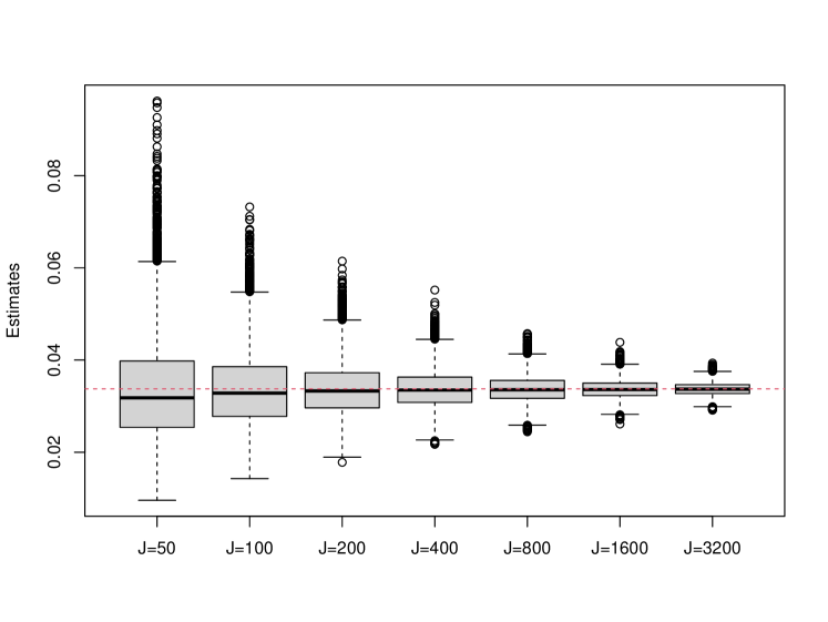
Figure 1: The boxplots of 1000 SMC estimates with different $J$ values of the probability $\Pr\{N(0,1]=1,N(1,2]=2\}$ for a Hawkes process $N$ with $\nu=1$, $\eta=0.6$, and a gamma excitation kernel with shape parameter 2 and scale parameter 0.1. The dashed horizontal line indicates the estimate of the probability via brute force Monte Carlo based on 100,000,000 simulated sample paths.

3.2 Approximate MLE via the Pseudo-Marginal Metropolis-Hastings (PMMH) MCMC

In this section, we use simulation experiments to investigate the finite sample performance of the PMMH-MCMC estimator of the model parameters. We simulate a Hawkes process with constant background intensity $\nu=2$, branching ratio $\eta=0.6$, and an exponential density kernel with scale or mean parameter $\beta=0.25$. The observation time points are evenly distributed between $0$ and $T=100$ or $T=200$ with constant spacing $\Delta=0.1,0.2,0.5$ or $1.0$. The different $\Delta$ values correspond to different levels of time coarsening. The number of particles in SMC likelihood approximation is set at $J=256$. The Hawkes process was simulated 500 times, and for each simulated sample path, only the values at the times $0,\Delta,2\Delta,\dotsc,T$ were observed and used in estimating the parameters $\theta=(\nu,\eta,\beta)$. In implementing the PMMH-MCMC, we used a Gaussian random walk proposal on the transformed parameters $(\log\nu,\log(\eta/(1-\eta)),\log\beta)$ with standard deviation $\sigma=0.05$. The constructed Markov Chain for the transformed parameter vector was initiated with a random draw from the 3-dimensional standard normal distribution and iterated a total of 50,000 times. For each parameter, the median of the Monte Carlo sample was taken as the value of the approximate MLE, the lower and upper 2.5 percentile points were taken as the lower and upper limits of the approximate 95% Wald confidence interval, and the difference of these two percentiles divided by $2\Phi^{-1}(0.975;0,1)\approx 3.92$ was taken as the estimate of the standard error (SE) of the approximate MLE. For comparison, the case $\Delta=0$ (with exact observations of event times) is also considered. Note that in this case, the exact log-likelihood can be computed, and so the MLE and its SE can be obtained by directly minimizing the negative log-likelihood function using general purpose numerical optimization routines and inverting the Hessian matrix. In our implementation, we used the optim function in R (R Core Team,, 2022) for numerical optimization with the loglikelihood function computed with the aid of the R package IHSEP (Chen,, 2022). The PMMH-MCMC estimator in the cases with $\Delta>0$ is implemented in julia (Bezanson et al.,, 2017).

The summary of the 500 estimates for each combination of $\Delta$ and $T$ are shown in Table 1, where (and whereafter) Est denotes the average of 500 MLE estimates, SE the empirical SE of the MLE calculated as the standard deviation of the 500 estimates, $\widehat{\mathrm{SE}}$ the average of the SE estimates, and CP the empirical coverage probability of the 95% Wald confidence interval calculated as the proportion of the 500 CIs that contain the corresponding true parameter value.

		$\nu=2$				$\eta=0.6$				$\beta=0.25$
T	$\Delta$	Est	SE	$\widehat{\mathrm{SE}}$	CP	Est	SE	$\widehat{\mathrm{SE}}$	CP	Est	SE	$\widehat{\mathrm{SE}}$	CP
100	0	2.053	0.2793	0.2849	0.954	0.586	0.0602	0.0608	0.952	0.248	0.0494	0.0472	0.914
200	0	2.022	0.2041	0.2026	0.948	0.596	0.0421	0.0430	0.948	0.252	0.0353	0.0335	0.952
100	0.1	2.039	0.3065	0.2946	0.942	0.593	0.0631	0.0635	0.944	0.256	0.0501	0.1104	0.946
200	0.1	2.005	0.2047	0.2041	0.952	0.600	0.0426	0.0433	0.960	0.256	0.0362	0.0353	0.944
100	0.2	2.046	0.3103	0.2932	0.932	0.591	0.0639	0.0631	0.944	0.255	0.0524	0.0540	0.944
200	0.2	2.005	0.2042	0.2034	0.938	0.600	0.0422	0.0434	0.960	0.255	0.0378	0.0363	0.940
100	0.5	2.054	0.3222	0.3036	0.936	0.590	0.0655	0.0651	0.954	0.254	0.0603	0.0642	0.956
200	0.5	2.006	0.2128	0.2085	0.936	0.600	0.0445	0.0444	0.960	0.255	0.0452	0.0421	0.934
100	1.0	2.086	0.3638	0.3144	0.910	0.583	0.0754	0.0671	0.912	0.242	0.0952	0.0834	0.926
200	1.0	2.014	0.2341	0.2108	0.906	0.598	0.0483	0.0446	0.924	0.253	0.0609	0.0603	0.896

Table 1: Summary of the parameter estimates in the simulation experiments.

The simulation results suggest that the estimators for all three parameters have performance similar to the MLE. For example, the empirical biases of the estimators are negligible compared to their respective standard errors. When the total observation time $T$ doubles, the standard errors all reduce roughly by a factor of 70% ($\approx 1/\sqrt{2}$). We also observe that as the degree of data coarsening intensifies, the empirical biases and standard errors of the estimators tend to increase. Meanwhile, the empirical coverage probabilities of the confidence intervals tend to decrease. This trend mirrors the growing difficulty the inference problem due to increasing level of information loss.

3.3 Comparison with existing methodologies

In this section we compare the performance of the proposed PMMH estimator with two competing methods in the literature, namely the maximum Whittle likelihood method of Cheysson and Lang, (2022) and the MCEM (Monte Carlo Expectation Maximization) method of Shlomovich et al., 2022b , by applying them on simulated data. The simulation models are the same as in the previous subsection. The 500 simulated data sets and the PMMH estimates for each of data coarsening level $\Delta\in\left\{0.1,0.2,0.5,1\right\}$ and total observation time $T\in\left\{100,200\right\}$ combination are also the same as before. The MCEM estimates based on the same simulated data sets for each of $\Delta$ and $T$ combination are computed using the Matlab code released by Shlomovich et al., 2022b at this link: https://github.com/lshlomovich/MCEM-Univariate-Hawkes. The Whittle likelihood estimates are computed using the whittle function in the R package hawkesbow by Cheysson, (2021). The boxplots showing the estimates for the three parameters by different methods with values of $\Delta$ and $T$ are shown in Figure 2.

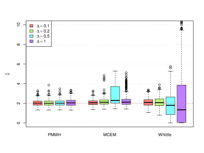
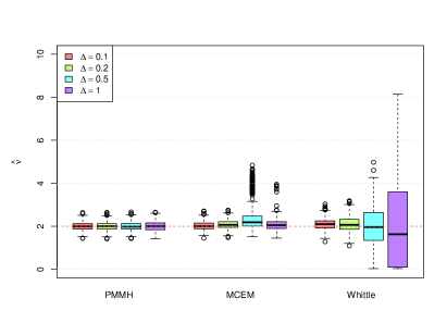
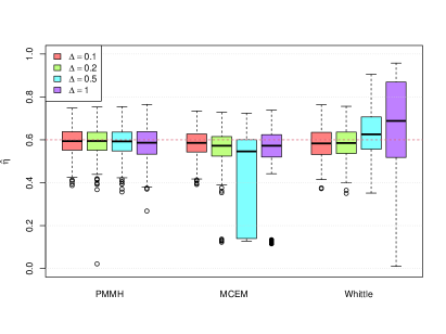
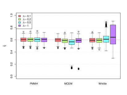
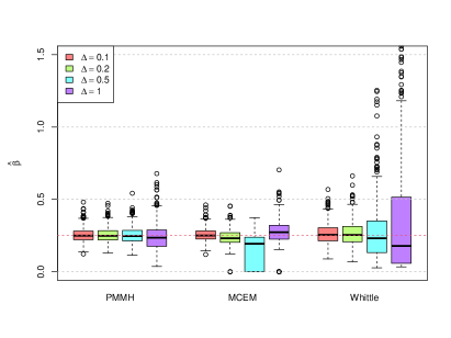
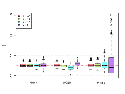
Figure 2: Boxplots of the estimates for the parameters of the Hawkes process with constant background intensity based on simulated data. Left panels: $T=100$, right panels: $T=200$; top panels: background intensity $\nu$, middle panels: branching ratio $\eta$, lower panels: the scale parameter $\beta$ of the exponential excitation kernel. The horizontal dashed lines indicate the true values of each parameter ($\nu=2$, $\eta=0.6$, $\beta=0.25$).

By Figure 2 it is fairly clear that when the data coarsening level is low, e.g. when $\Delta=0.1$, all three estimators have more or less the same performance. However, when the level of data coarsening increases, the PMMH estimator tends to perform better than the MCEM and Whittle estimators in terms of both bias and variance. When $\Delta=0.5$, the body of the boxplot for the MCEM estimates for each of the parameters seems to lie entirely on one side of the true value of the corresponding parameter, even with the larger total observation time, suggesting significant bias of the MCEM estimator. On the other hand, the Whittle estimator for each of the three parameters shows rather large variance compared with the other two estimators, although its bias seems negligible relative to its standard deviation. The larger variances of the Whittle estimator suggest that it is less efficient than the likelihood based PMMH estimator. The bias of the MCEM estimators of Shlomovich et al., 2022b might be due to the way they estimated the Q-function, or the conditional expectation of the complete-data log-likelihood function given the observed data, in the E- (Expectation-) step of the EM cycle using Monte Carlo method. Rather than taking a random sample from the proposal distribution and using the importance-weighted sample to approximate the conditional distribution of the hidden state, they calculated the most likely state(s) according to the proposal distribution and used the importance-weighted states to approximated the needed conditional distribution of the hidden state. While it intuitively makes sense, there is no guarantee that this method leads to unbiased estimate of the Q-function in the E-step of the EM algorithm, and it seems that the bias here has been inherited by their final estimator of the model parameters.

4 Application

In this section we apply the proposed estimation method to an infectious disease dataset previously studied by Cheysson and Lang, (2022). The dataset contains the weekly counts of measles cases in Tokyo Japan during the 393-week period from 10 Aug 2012 to 20 Feb 2020. The weekly measles cases counts vary between 0 and 10, with an average of 0.67, a median of 0.0, and a standard deviation of 1.38. A graph of the weekly case counts against week end date is show in Figure 3. Cheysson and Lang, (2022)

Figure 3: Time series plot of the weekly measles case counts in Tokyo Japan from 2012-08-10 to 2020-02-20.

assumed a non-causal Hawkes process with a constant background event intensity and a Gaussian kernel for the underlying point process of measles cases and applied the maximum Whittle likelihood estimator to estimate the model parameters. They estimated a background intensity of 0.04 day^-1, a branching ratio of 0.72, and a mean and standard deviation for the Gaussian excitation kernel 9.8 days and 5.9 days respectively. They also used formal tests to confirm the fitted non-causal Hawkes process provides acceptable fit to the data.

While the fitted non-causal Hawkes process of Cheysson and Lang, (2022) can reproduce the spectral features of the data, some of the appealing features of the classical (causal) Hawkes process is comprised. For example, the conditional intensity process relatively to the natural filtration induced by the underlying point process, which is easily available in the classical Hawkes process, is not tractable anymore. In this work, we fit a causal Hawkes process with an exponential kernel function to the same dataset using the PMMH-MCMC method. We initialise the Markov chain with a random starting point as in the simulation experiments and iterate the chain for a total of 11000 time steps. Again, we use the random walk Gaussian proposal on the transformed parameter vector with a standard deviation of 0.05. The number of particles used in the estimation of the log-likelihood function is also the same as in the simulation experiments, namely $J=256$. From the trace plots of the log-likelihood estimate and the MCMC draw in Figure 4, it is clear that the Markov chain has reached convergence after around 1000 iterations.

Figure 4: Trace plots of the log-likelihood estimate and the parameter values (different dimensions of the MCMC draw).

Extracting the appropriate quantiles of the next 10,000 MCMC draws, we obtained the point estimates and 95% confidence intervals (in brackets) for the three parameters as follows: $\widehat{\nu}=0.0244\ ([0.0155,0.0323])$, $\widehat{\eta}=0.749\ ([0.625,0.882])$, and $\widehat{\beta}=8.34\ ([5.99,12.45])$. Note that with these parameter estimates, the expected number of events per 7-day period should be $\widehat{\nu}/(1-\widehat{\eta})\times 7\approx 0.680$, which is fairly close to the average weekly case count of $0.672$. In contrast, by the estimates of Cheysson and Lang, (2022), the expected weekly number of cases would be $0.04/(1-0.72)\times 7=1.0$, which is substantially higher than the corresponding average in the data. The expected number of imported cases by our model is $\widehat{\nu}\times 393\times 7\approx 67$, or 25.4% of the 264 cases in total, which is slightly lower than the estimated percentage of $28\%$ by Cheysson and Lang,’s non-causal Hawkes process model, but is closer to the finding of a previous study by Nishiura et al., (2017), in which 23 among 103 confirmed cases were found to be imported cases.

To assess whether the fitted Hawkes process model is adequate for the observed data, we simulated 1000 times the discretely observed sample path of the fitted model and compare the simulated paths with the actual sample path implied by the data. The left panel of Figure 5 shows the 1000 simulated paths of the fitted model together with the observed path. We note that the actual path stays between the (pointwise) lower and upper 2.5 percentiles of the simulated paths, suggesting the fitted model is adequate for the weekly measles case count data. For comparison, we also simulated 1000 paths of the non-causal Hawkes process of Cheysson and Lang, and graph them together with the actual path in the right panel of Figure 5. The actual path wanders out of the 2.5 percentile lines for a substantial amount of time, suggesting the non-causal Hawkes process is not adequate for the observed data. The comparison suggests that the classical Hawkes process with an exponential excitation kernel can offer adequate and better fit to the data than the non-causal Hawkes process, despite having one parameter less.

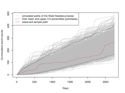
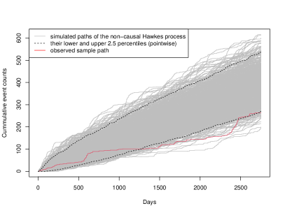
Figure 5: Simulated sample paths of the fitted Hawkes process models together with the actual path. Left: the Hawkes process with an exponential kernel; right: the (non-causal) Hawkes process with a Gaussian kernel.

To entertain the possibility a kernel with a peak away from 0 might fit the data better than an exponential kernel, we also fitted Hawkes processes with Weibull and gamma density kernels to the data. In addition to the scale parameter $\beta$, both kernels have an extra parameter $\alpha\ (>0)$ that regulates the shape of the kernel. When the shape parameter $\alpha$ is bigger than 1, both kernels will have a peak away from zero; when the shape parameter is equal to 1, both kernels reduce to the exponential kernel; and when the shape parameter is less than 1, both kernels are decreasing on the positive real line and approach infinity at zero. The fitted Hawkes processes with both kernels have a shape parameter smaller than 1, with very marginal improvement in the log-likelihood value. For example, with the Weibull kernel $\alpha(\cdot/\beta)^{\alpha-1}\exp(-(\cdot/\beta)^{\alpha})1\{\cdot>0\}$, the parameter estimates are $\widehat{\nu}=0.0204\ ([0.0112,0.0303])$, $\widehat{\eta}=0.788\ ([0.0644,0.903])$, $\widehat{\alpha}=0.742\ ([0.518,1.061]])$, and $\widehat{\beta}=9.43\ ([6.29,14.31])$, and the log-likelihood value at $(\widehat{\nu},\widehat{\eta},\widehat{\alpha},\widehat{\beta})$ is $-379.83$ $([-380.10,-379.54])$, which is only a very minor improvement from the log-likelihood value of $-380.19$ $([-380.47,-379.90])$ for the fitted model with the exponential kernel. Therefore, there does not appear to be statistical evidence to support a kernel with a peak away from zero for the Hawkes process model.

5 Discussion

The main contribution of our work is the proposal of an unbiased sequential Monte Carlo estimator of the intractable likelihood of the Hawkes process relative to a discretely observed sample path and an illustration of its usefulness in estimating the parameters of the Hawkes process from such data when combined with the pseudo marginal Metropolis-Hastings(PMMH) algorithm. In our numerical experiments, the resulting estimator outforms two competitive estimators proposed in the literature in terms of mean square error and behaves much like the maximum likelihood estimator (MLE). Our method also gives the standard errors of the estimators as a by-product.

While the pseudo marginal Metropolis-Hastings (PMMH) algorithm works very well in our numerical experiments with farily arbitrary choices for the number of particles and the step size of the Gaussian random walk proposal, it is likely that computationally more efficient procedures can be obtained by following the advices in the literature on how to choose these tuning parameters optimally, such as Pitt et al., (2012); Doucet et al., (2015); Gelman et al., (1997). Moreover, there have also been more efficient variants of the PMMH algorithms such as the correlated pseudomarginal method of Deligiannidis and Doucet, (2018) and the unbiased Markov Chain Monte Carlo method of Middleton et al., (2020). Improvement of the computational efficiency of our estimation procedure will is interesting future work.

Justification of the use of the centre of the likelihood distribution or more generally, the posterior distribution in a Bayesian framework, for the model parameter to approximate the MLE relies on the consistency and asymptotically normality expected of the MLE. While there is strong empirical evidence to support these expected properties of the MLE in the current context, a formal proof of such properties is needed and shall be pursued elsewhere.
Acknowledgement This work has benefited from discussions with with Prof Pierre del Moral and Prof Judith Rousseau, for which we are grateful. Part of the work was done while FC was visiting the University of Oxford on a sabbatical trip. The hospitality of Prof Samuel Cohen and Prof Judith Rousseau, the Oxford-Man Institute of Quantitative Finance, the Mathematical Institute and the Department of Statistics is gratefully acknowledged. We also wish to thank Prof Xiaoli Meng for bringing relevant references to our attention. This research includes computations using the computational cluster Katana supported by Research Technology Services at UNSW Sydney, as well as resources and services at the National Computational Infrastructure and the Pawsey Supercomputing Centre, both supported by the Australian Government’s National Collaborative Research Infrastructure Strategy (NCRIS). This research was supported by the Australian Government through the Australian Research Council (project number DP240101480).

Appendices

Appendix A Proof of the unbiasedness of the bootstrap particle approximation of the likelihood function

Proof.

For ease of presentation, we use slightly more generic notation here. Let $y_{1:n}=(y_{1},\dotsc,y_{n})$ denote the time series of observations and $x_{1:n}=(x_{1},\dotsc,x_{n})$ the sequence of hidden states. Note that the $y_{i}$’s can have different dimensions, and so can the $x_{i}$’s. The bootstrap particle approximation to the likelihood $p(y_{1:n})$ presented in this work takes the form:

$$\widehat{p}(y_{1:n}) =\prod_{i=1}^{n}\widehat{p}(y_{i}|y_{1:i-1})\equiv\prod_{i=1}^{n}\frac{1}{J}\sum_{j=1}^{J}W_{i}^{(j)},$$

where

$$W_{i}^{(j)}=p(y_{i}|y_{1:i-1},x_{1:i,i}^{(j)})\bigg{[}\frac{P(\,\mathrm{d}x_{i}|x_{1:i-1,i}^{(j)},y_{1:i-1})}{Q(\,\mathrm{d}x_{i}|x_{1:i-1,i}^{(j)},y_{1:i})}\bigg{]}_{x_{i}=x_{i,i}^{(j)}},$$

and

$$x_{1:i,i}^{(1:J)}\stackrel{{\scriptstyle\mathrm{i.i.d.}}}{{\sim}}\frac{\frac{1}{J}\sum_{j=1}^{J}W_{i-1}^{(j)}\delta_{x_{1:i-1,i-1}^{(j)}}(\,\mathrm{d}x_{1:i-1})}{\widehat{p}(y_{i-1}|y_{1:i-2})}Q(\,\mathrm{d}x_{i}|x_{1:i-1},y_{1:i-1}).$$

By our definition of the SMC approximation and the tower property of conditional expectations,

$$\mathbb{E}\left[\widehat{p}(y_{i}|y_{1:i-1})\big{|}x_{1:l,l}^{(1:J)},l=1,\dotsc,i-1\right]$$

$${}={} \mathbb{E}\left[\widehat{p}(y_{i}|y_{1:i-1})\big{|}x_{1:i-1,i-1}^{(1:J)}\right]$$

$${}={} \mathbb{E}\left[\mathbb{E}\left[\widehat{p}(y_{i}|y_{1:i-1})\big{|}x_{1:i-1,i}^{(1:J)},x_{1:i-1,i-1}^{(1:J)}\right]\Big{|}x_{1:i-1,i-1}^{(1:J)}\right]$$

$${}={} \mathbb{E}\left[\mathbb{E}\left[\frac{1}{J}\sum_{j=1}^{J}p(y_{i}|y_{1:i-1},x_{1:i,i}^{(j)})\Big{[}\frac{P(\,\mathrm{d}x_{i}|x_{1:i-1,i}^{(j)},y_{1:i-1})}{Q(\,\mathrm{d}x_{i}|x_{1:i-1,i}^{(j)},y_{1:i})}\Big{]}_{x_{i}=x_{i,i}^{(j)}}\Big{|}x_{1:i-1,i}^{(1:J)},x_{1:i-1,i-1}^{(1:J)}\right]\bigg{|}x_{1:i-1,i-1}^{(1:J)}\right]$$

$${}={} \mathbb{E}\left[\frac{1}{J}\sum_{j=1}^{J}\mathbb{E}\left[p(y_{i}|y_{1:i-1},x_{1:i,i}^{(j)})\Big{[}\frac{P(\,\mathrm{d}x_{i}|x_{1:i-1,i}^{(j)},y_{1:i-1})}{Q(\,\mathrm{d}x_{i}|x_{1:i-1,i}^{(j)},y_{1:i})}\Big{]}_{x_{i}=x_{i,i}^{(j)}}\Big{|}x_{1:i-1,i}^{(1:J)},x_{1:i-1,i-1}^{(1:J)}\right]\bigg{|}x_{1:i-1,i-1}^{(1:J)}\right]$$

$${}={} \mathbb{E}\left[\frac{1}{J}\sum_{j=1}^{J}\int p(y_{i}|y_{1:i-1},x_{1:i-1,i}^{(j)},x_{i})\Big{[}\frac{P(\,\mathrm{d}x_{i}|x_{1:i-1,i}^{(j)},y_{1:i-1})}{Q(\,\mathrm{d}x_{i}|x_{1:i-1,i}^{(j)},y_{1:i})}\Big{]}Q(\,\mathrm{d}x_{i}|x_{1:i-1,i}^{(j)},y_{1:i})\bigg{|}x_{1:i-1,i-1}^{(1:J)}\right]$$

$${}={} \mathbb{E}\left[\frac{1}{J}\sum_{j=1}^{J}\int p(y_{i}|y_{1:i-1},x_{1:i-1,i}^{(j)},x_{i})P(\,\mathrm{d}x_{i}|x_{1:i-1,i}^{(j)},y_{1:i-1})\bigg{|}x_{1:i-1,i-1}^{(1:J)}\right]$$

$${}={} \mathbb{E}\left[\frac{1}{J}\sum_{j=1}^{J}p(y_{i}|y_{1:i-1},x_{1:i-1,i}^{(j)})\big{|}x_{1:i-1,i-1}^{(1:J)}\right].$$

Conditional on $x_{1:i-1,i-1}^{(1:J)}$, the $x_{1:i-1,i}^{(j)},\ j=1,\dots,J$ are $\mathrm{i.i.d.}$ multinomial and each of them takes the value $x_{1:i-1,i-1}^{(j)}$ with probability $\frac{1}{J}W_{i-1}^{(j)}/\widehat{p}(y_{i-1}|y_{1:i-2})$, $j=1,\dotsc,J$. Therefore,

$$\mathbb{E}\left[\widehat{p}(y_{i}|y_{1:i-1})\big{|}x_{1:l,l}^{(1:J)},l=1,\dotsc,i-1\right]$$

$${}={} \mathbb{E}\left[p(y_{i}|y_{1:i-1},x_{1:i-1,i}^{(1)})\big{|}x_{1:i-1,i-1}^{(1:J)}\right]$$

$${}={} \frac{\frac{1}{J}\sum_{j=1}^{J}p(y_{i}|y_{1:i-1},x_{1:i-1,i-1}^{(j)})W_{i-1}^{(j)}}{\widehat{p}(y_{i-1}|y_{1:i-2})}$$

$${}={} \frac{\frac{1}{J}\sum_{j=1}^{J}p(y_{i}|y_{1:i-1},x_{1:i-1,i-1}^{(j)})p(y_{i-1}|y_{1:i-2},x_{1:i-1,i-1}^{(j)})\Big{[}\frac{P(\,\mathrm{d}x_{i-1}|x_{1:i-2,i-1}^{(j)},y_{1:i-2})}{Q(\,\mathrm{d}x_{i-1}|x_{1:i-2,i-1}^{(j)},y_{1:i-1})}\Big{]}_{x_{i-1}=x_{i-1,i-1}^{(j)}}}{\widehat{p}(y_{i-1}|y_{1:i-2})}$$

$${}={} \frac{\frac{1}{J}\sum_{j=1}^{J}p(y_{i-1:i}|y_{1:i-2},x_{1:i-1,i-1}^{(j)})\Big{[}\frac{P(\,\mathrm{d}x_{i-1}|x_{1:i-2,i-1}^{(j)},y_{1:i-2})}{Q(\,\mathrm{d}x_{i-1}|x_{1:i-2,i-1}^{(j)},y_{1:i-1})}\Big{]}_{x_{i-1}=x_{i-1,i-1}^{(j)}}}{\widehat{p}(y_{i-1}|y_{1:i-2})}.$$

From this, and by double expectation, we have

$$\mathbb{E}\left[\widehat{p}(y_{1:n})\right]$$

$${}={} \mathbb{E}\left[\mathbb{E}\left[\prod_{i=1}^{n}\widehat{p}(y_{i}|y_{1:i-1})\Big{|}x_{1:l,l}^{(1:J)},l=1,\dotsc,n-1\right]\right]$$

$${}={} \mathbb{E}\left[\prod_{i=1}^{n-1}\widehat{p}(y_{i}|y_{1:i-1})\mathbb{E}\left[\widehat{p}(y_{n}|y_{1:n-1})\Big{|}x_{1:n-1,n-1}^{(1:J)}\right]\right]$$

$${}={} \mathbb{E}\left[\prod_{i=1}^{n-2}\widehat{p}(y_{i}|y_{1:i-1})\frac{1}{J}\sum_{j=1}^{J}p(y_{n-1:n}|y_{1:n-2},x_{1:n-1,n-1}^{(j)})\Big{[}\frac{P(\,\mathrm{d}x_{n-1}|x_{1:n-2,n-1}^{(j)},y_{1:n-2})}{Q(\,\mathrm{d}x_{n-1}|x_{1:n-2,n-1}^{(j)},y_{1:n-1})}\Big{]}_{x_{n-1}=x_{n-1,n-1}^{(j)}}\right].$$

Now, by conditioning on $x_{1:l,l}^{(1:J)},l=1,\dotsc,n-2$, we have

$$\mathbb{E}\left[\widehat{p}(y_{1:n})\right]$$

$${}={} \mathbb{E}\left[\prod_{i=1}^{n-3}\widehat{p}(y_{i}|y_{1:i-1})\frac{1}{J}\sum_{j=1}^{J}p(y_{n-2:n}|y_{1:n-3},x_{1:n-2,n-2}^{(j)})\Big{[}\frac{P(\,\mathrm{d}x_{n-2}|x_{1:n-3,n-2}^{(j)},y_{1:n-3})}{Q(\,\mathrm{d}x_{n-2}|x_{1:n-3,n-2}^{(j)},y_{1:n-2})}\Big{]}_{x_{n-2}=x_{n-2,n-2}^{(j)}}\right].$$

Repeating this process, we have

$$\mathbb{E}\left[\widehat{p}(y_{1:n})\right]$$

$${}={} \mathbb{E}\left[\frac{1}{J}\sum_{j=1}^{J}p(y_{1:n}|x_{1,1}^{(j)})\Big{[}\frac{P(\,\mathrm{d}x_{1})}{Q(\,\mathrm{d}x_{1}|y_{1})}\Big{]}_{x_{1}=x_{1,1}^{(j)}}\right]$$

$${}={} \mathbb{E}\left[p(y_{1:n}|x_{1,1}^{(1)})\Big{[}\frac{P(\,\mathrm{d}x_{1})}{Q(\,\mathrm{d}x_{1}|y_{1})}\Big{]}_{x_{1}=x_{1,1}^{(1)}}\right]$$

$${}={} \int p(y_{1:n}|x_{1})\Big{[}\frac{P(\,\mathrm{d}x_{1})}{Q(\,\mathrm{d}x_{1}|y_{1})}\Big{]}Q(\,\mathrm{d}x_{1}|y_{1})$$

$${}={} \int p(y_{1:n}|x_{1})P(\,\mathrm{d}x_{1})$$

$${}={} p(y_{1:n}).\qed$$

Appendix B Proof of the exactness of the MCMC approximation to the likelihood distribution

Proof.

Write the SMC likelihood approximation $\widehat{L}(\theta,u)$ to remind us of its dependence on the Monte Carlo randomness $u$, which can be taken as a uniform random variable on the interval $(0,1)$ (see e.g. Kallenberg,, 2021, Lemma 4.22). The Markov chain $\theta^{(1)},\theta^{(2)},\dotsc$ we constructed using the PMMH algorithm to approximate the likelihood distribution $L(\theta)\,\mathrm{d}\theta/\int L(\theta)\,\mathrm{d}\theta$ can be viewed as the second to last dimension of the Markov chain $(u^{(i)},\theta^{(i)})$, $i=1,2,\dotsc$ with transition kernel

$$K((\,\mathrm{d}u^{\prime},\,\mathrm{d}\theta^{\prime})|(u,\theta))=\,\mathrm{d}u^{\prime}Q(\,\mathrm{d}\theta^{\prime}|\theta)\left[\frac{\widehat{L}(\theta^{\prime},u^{\prime})\,\mathrm{d}\theta^{\prime}Q(\,\mathrm{d}\theta|\theta^{\prime})}{\widehat{L}(\theta,u)\,\mathrm{d}\theta Q(\,\mathrm{d}\theta^{\prime}|\theta)}\wedge 1\right]+R(u,\theta)\delta_{(u,\theta)}(\,\mathrm{d}u^{\prime},\,\mathrm{d}\theta^{\prime}),$$

where $x\wedge y=\min\left\{x,y\right\}$ and $R(u,\theta)=1-\iint\left[\frac{\widehat{L}(\theta^{\prime},u^{\prime})\,\mathrm{d}\theta^{\prime}Q(\,\mathrm{d}\theta|\theta^{\prime})}{\widehat{L}(\theta,u)\,\mathrm{d}\theta Q(\,\mathrm{d}\theta^{\prime}|\theta)}\wedge 1\right]\,\mathrm{d}u^{\prime}Q(\,\mathrm{d}\theta^{\prime}|\theta)$. For $(u,\theta)\neq(u^{\prime},\theta^{\prime})$, we note

$$\,\mathrm{d}u\,\widehat{L}(\theta,u)\,\mathrm{d}\theta\,K((\,\mathrm{d}u^{\prime},\,\mathrm{d}\theta^{\prime})|(u,\theta))$$

$${}={} \,\mathrm{d}u\,\widehat{L}(\theta,u)\,\mathrm{d}\theta\,\mathrm{d}u^{\prime}Q(\,\mathrm{d}\theta^{\prime}|\theta)\left[\frac{\widehat{L}(\theta^{\prime},u^{\prime})\,\mathrm{d}\theta^{\prime}Q(\,\mathrm{d}\theta|\theta^{\prime})}{\widehat{L}(\theta,u)\,\mathrm{d}\theta Q(\,\mathrm{d}\theta^{\prime}|\theta)}\wedge 1\right]$$

$${}={} \,\mathrm{d}u\,\,\mathrm{d}u^{\prime}\widehat{L}(\theta^{\prime},u^{\prime})\,\mathrm{d}\theta^{\prime}Q(\,\mathrm{d}\theta|\theta^{\prime})\ \wedge\ \,\mathrm{d}u\,\widehat{L}(\theta,u)\,\mathrm{d}\theta\,\mathrm{d}u^{\prime}Q(\,\mathrm{d}\theta^{\prime}|\theta)$$

$${}={} \,\mathrm{d}u^{\prime}\,\widehat{L}(\theta^{\prime},u^{\prime})\,\mathrm{d}\theta^{\prime}\,K((\,\mathrm{d}u,\,\mathrm{d}\theta)|(u^{\prime},\theta^{\prime})),$$

and therefore $\,\mathrm{d}u\widehat{L}(\theta,u)\,\mathrm{d}\theta/\iint\widehat{L}(\theta,u)\,\mathrm{d}\theta\,\mathrm{d}u$ is the invariant distribution of the extended chain $(u^{(i)},\theta^{(i)}),i=1,2,\dotsc$. The $\theta$-marginal of this invariant distribution is

$$\left[\int\widehat{L}(\theta,u)\,\mathrm{d}u\right]\,\mathrm{d}\theta\Big{/}\iint\widehat{L}(\theta,u)\,\mathrm{d}\theta\,\mathrm{d}u=L(\theta)\,\mathrm{d}\theta\Big{/}\int L(\theta)\,\mathrm{d}\theta$$

by Proposition 1. This shows that, as the $\theta$-marginal of the extended chain, $\theta^{(i)},i=1,2,\dotsc,$ has the likelihood distribution as its invariant distribution. ∎

References

- Andrieu et al., (2010) Andrieu, C., Doucet, A., and Holenstein, R. (2010). Particle markov chain monte carlo methods. Journal of the Royal Statistical Society: Series B (Statistical Methodology), 72(3):269–342.
- Andrieu and Roberts, (2009) Andrieu, C. and Roberts, G. O. (2009). The pseudo-marginal approach for efficient Monte Carlo computations. The Annals of Statistics, 37(2):697 – 725.
- Bezanson et al., (2017) Bezanson, J., Edelman, A., Karpinski, S., and Shah, V. B. (2017). Julia: A fresh approach to numerical computing. SIAM review, 59(1):65–98.
- Chen, (2022) Chen, F. (2022). IHSEP: Inhomogeneous Self-Exciting Process. R package version 0.3.1. URL: https://cran.r-project.org/package=IHSEP.
- Cheysson, (2021) Cheysson, F. (2021). hawkesbow: Estimation of Hawkes Processes from Binned Observations. R package version 1.0.2.
- Cheysson and Lang, (2022) Cheysson, F. and Lang, G. (2022). Spectral estimation of Hawkes processes from count data. The Annals of Statistics, 50(3):1722 – 1746.
- Chornoboy et al., (1988) Chornoboy, E., Schramm, L., and Karr, A. (1988). Maximum likelihood identification of neural point process systems. Biological Cybernetics, 59(4):265–275.
- Daley and Vere-Jones, (2003) Daley, D. J. and Vere-Jones, D. (2003). An Introduction to the Theory of Point Processes Volume I: Elementary Theory and Methods. Springer-Verlag, New York, 2nd edition.
- Deligiannidis and Doucet, (2018) Deligiannidis, G. and Doucet, A. (2018). The correlated pseudomarginal method. Journal of the Royal Statistical Society. Series B (Statistical Methodology), 80(5):pp. 839–870.
- Doucet et al., (2015) Doucet, A., Pitt, M. K., Deligiannidis, G., and Kohn, R. (2015). Efficient implementation of Markov chain Monte Carlo when using an unbiased likelihood estimator. Biometrika, 102(2):295–313.
- Gelman et al., (1997) Gelman, A., Gilks, W. R., and Roberts, G. O. (1997). Weak convergence and optimal scaling of random walk Metropolis algorithms. The Annals of Applied Probability, 7(1):110 – 120.
- Gordon et al., (1993) Gordon, N., Salmond, D., and Smith, A. (1993). Novel approach to nonlinear/non-Gaussian Bayesian state estimation. IEE Proceedings F - Radar and Signal Processing, 140:107–113(6).
- Hastings, (1970) Hastings, W. K. (1970). Monte Carlo sampling methods using Markov chains and their applications. Biometrika, 57(1):97–109.
- Hawkes, (1971) Hawkes, A. G. (1971). Spectra of some self-exciting and mutually exciting point processes. Biometrika, 58(1):83–90.
- Kallenberg, (2021) Kallenberg, O. (2021). Foundations of Modern Probability. Springer Nature, Switzerland, 3rd edition.
- Kitagawa, (1996) Kitagawa, G. (1996). Monte carlo filter and smoother for non-gaussian nonlinear state space models. Journal of Computational and Graphical Statistics, 5(1):1–25.
- Metropolis et al., (1953) Metropolis, N., Rosenbluth, A. W., Rosenbluth, M. N., Teller, A. H., and Teller, E. (1953). Equation of state calculations by fast computing machines. The Journal of Chemical Physics, 21(6):1087–1092.
- Middleton et al., (2020) Middleton, L., Deligiannidis, G., Doucet, A., and Jacob, P. E. (2020). Unbiased Markov chain Monte Carlo for intractable target distributions. Electronic Journal of Statistics, 14(2):2842 – 2891.
- Nishiura et al., (2017) Nishiura, H., Mizumoto, K., and Asai, Y. (2017). Assessing the transmission dynamics of measles in japan, 2016. Epidemics, 20:67–72.
- Ogata, (1978) Ogata, Y. (1978). The asymptotic behaviour of maximum likelihood estimators for stationary point processes. Annals of the Institute of Statistical Mathematics, 30:243–261.
- Ozaki, (1979) Ozaki, T. (1979). Maximum likelihood estimation of Hawkes’ self-exciting point processes. Annals of the Institute of Statistical Mathematics, 31(1):145–155.
- Pitt et al., (2012) Pitt, M. K., dos Santos Silva, R., Giordani, P., and Kohn, R. (2012). On some properties of markov chain monte carlo simulation methods based on the particle filter. Journal of Econometrics, 171(2):134–151. Bayesian Models, Methods and Applications.
- Pitt and Shephard, (1999) Pitt, M. K. and Shephard, N. (1999). Filtering via simulation: Auxiliary particle filters. Journal of the American Statistical Association, 94(446):590–599.
- R Core Team, (2022) R Core Team (2022). R: A Language and Environment for Statistical Computing. R Foundation for Statistical Computing, Vienna, Austria.
- Rizoiu et al., (2022) Rizoiu, M.-A., Soen, A., Li, S., Calderon, P., Dong, L. J., Menon, A. K., and Xie, L. (2022). Interval-censored hawkes processes. Journal of Machine Learning Research, 23(338):1–84.
- Shcherbinin, (1987) Shcherbinin, A. F. (1987). The normalized likelihood method. Measurement Techniques, 30(12):1129–1134.
- (27) Shlomovich, L., Cohen, E. A. K., and Adams, N. (2022a). A parameter estimation method for multivariate binned Hawkes processes. Statistics and Computing, 32(6):98.
- (28) Shlomovich, L., Cohen, E. A. K., Adams, N., and Patel, L. (2022b). Parameter estimation of binned Hawkes processes. Journal of Computational and Graphical Statistics, 31(4):990–1000.
- van der Vaart, (2007) van der Vaart, A. (2007). Asymptotic Statistics. Cambridge university press, New York.
- Xie and Singh, (2013) Xie, M.-g. and Singh, K. (2013). Confidence distribution, the frequentist distribution estimator of a parameter: A review. International Statistical Review, 81(1):3–39.