Bexcitonics: Quasi-particle approach to open quantum dynamics
Abstract
We isolate a class of exact quantum master equations (EQMEs) to capture the dynamics of open quantum systems coupled to bosonic thermal baths of arbitrary complexity. This is done by mapping this dynamics into that of the system in interaction with a few collective bath excitations or bexcitons. The bexcitons emerge from a decomposition of the bath correlation function. Their properties, while unphysical, offer a coarse-grained view of the correlated system-bath dynamics that can be used to design efficient EQMEs. The approach provides a systematic strategy to construct EQMEs that include the system-bath coupling to all orders even for non-Markovian environments and contains the well-known hierarchical equation of motion method as a special case.
I Introduction
A central challenge in the physical sciences is to accurately capture the quantum dynamics of atoms, molecules and other quantum systems when they interact with quantum thermal environments [1, 2, 3, 4, 5, 6, 7]. This is needed, for example, to develop better organic solar cells [8], understand vital processes such as photosynthesis [9], and to advance quantum technologies for computing, sensing and communication [10, 11]. Several strategies have been developed to follow this open quantum system dynamics through quantum master equations (QMEs) that implicitly capture the influence of the quantum bath on the system. In particular, important progress has been made for bosonic environments [12, 13, 14, 15, 16, 17, 18, 5, 19]. These environments are ubiquitous because any quantum environment can be mapped into a collection of bosons provided the system-bath interaction can be captured to second order in perturbation theory [20, 21, 22], and this situation is common in the condensed phase [23, 13] where system-bath interactions are diluted over a macroscopic number of degrees of freedom.
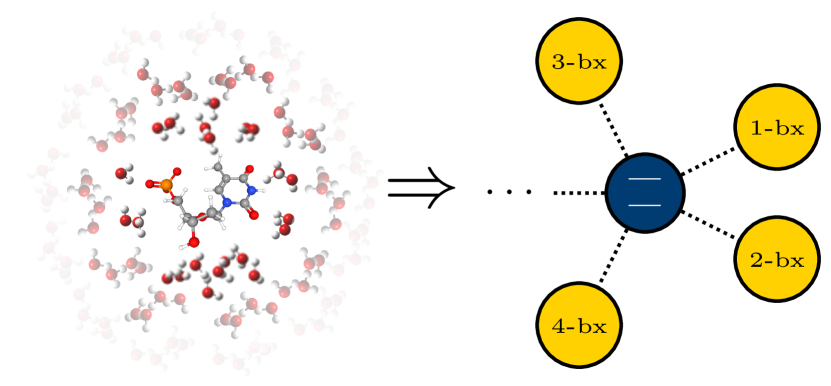
In this paper, we isolate a class of exact QMEs (EQMEs) that map the dynamics of quantum systems immersed in thermal bosonic environments of arbitrary complexity into a computationally tractable scheme where the system is in interaction with a few collective bath excitations, or bexcitons (see Fig. 1). The bexcitons are fictitious quasiparticles that arise from a decomposition of the bath correlation function into distinct features, and are created and destroyed as the system decoheres. While in QMEs the environment’s dynamics is not followed explicitly, in this bexcitonic picture it is captured in a coarse-grained way offering additional tools to understand the system–bath entanglement and numerical convergence of the EQME. The approach clarifies the underlying structure of the open quantum dynamics and can be used to develop efficient propagation schemes and EQMEs with optimal convergence properties. Importantly, the scheme admits arbitrary time-dependence in the system’s Hamiltonian as needed to characterize driven open quantum systems.
Our theory can be seen as a generalization of the numerically exact Hierarchical Equations of Motion (HEOM) [24, 12, 25, 26, 27, 5], which is one of the most powerful numerical methods to simulate the open quantum dynamics. In fact, our developments recover HEOM variants as specific cases and show that they emerge from a common bexcitonic picture.
Another quasiparticle view of open quantum dynamics is that offered by the effective Hamiltonian method [17, 7, 28] where a small number of unphysical dissipative harmonic modes are coupled to the system in such a way that they recover the physical dynamics. This method is best suited for underdamped Brownian environments and requires further techniques for Ohmnic environments [29]. By contrast, our EQMEs can exactly treat both overdamped and underdamped environments, Markovian and non-Markovian dynamics, weak and strong system-bath correlations, in a unified form by propagating the dynamics in bexcitonic space. Further, since the approach avoids invoking perturbation theory in the system-bath interaction, it goes beyond all methods based on perturbative expansions such as the Lindblad and Redfield equations [30, 31, 32].
II Theory
As customary, we decompose the Hamiltonian of a quantum system in interaction with an environment , into the system , the bath , and their interaction . The system can be subject to arbitrary time-dependence, such as that introduced by light-matter interactions. For bosonic baths, where is the frequency of the -th mode and its raising and its lowering operator (). For simplicity, we focus on with only one coupling term but the final results are readily extendable to many coupling terms. Here is a system’s operator and a collective bath coordinate with coupling strength to the -th mode. Throughout we use atomic units where .
We begin from the exact dynamical map of the system’s reduced density matrix at time from initial state [26]. For convenience we use the notation and for the ordering of matrix multiplications, and and for the symmetric and anti-symmetric super-operator generated from . Dynamical maps require the overall density matrix to be initially in a separable state . We take to be the thermal density matrix of the bath, where , the temperature, the bath partition function, and denotes a trace over bath degrees of freedom. While the dynamics of is unitary, the dynamics of is non-unitary and satisfies [26]
| (1) |
where is the time-ordering operator,
| (2) |
and is the bath correlation function (BCF). In writing Eq. (1) we have adopted the interaction picture of , where . Equation (2) provides a formal solution to the open quantum dynamics at all temperatures and to all orders in the system-bath interaction. As seen, contains all the information needed to capture the influence of the bath on .
II.1 Identifying dynamical features of the bath correlation function
To make this formal solution computationally tractable, we decompose and its conjugate as
| (3) |
where is a complex basis and , are time-independent complex expansion coefficients. Each component of the basis defines a feature of the bath and is required to satisfy
| (4) |
The first condition guarantees that spans a function space that contains both and its time-derivative, as needed for dynamics. The second one reflects that physical systems have non-zero quantum fluctuations. The dimension of this basis defines the number of bath features. As discussed below, this decomposition is general but not unique.
Any basis satisfying Eq. (4) can be used to decompose the BCF into features. We now show a systematic, albeit not unique, way to do this that demonstrate Eq. (3) is general, and that yields features satisfying for . The structure of the bath is captured by its spectral density (), a quantity that summarizes the frequencies of the environment and its interaction strength to the system. The BCF is related to through [33, 4]
| (5) |
where is an odd extension of and is the Bose-Einstein distribution. We evaluate Eq. (5) using the residue theorem through analytical continuation and expanding through a Padé [34] or Matsubara [35] schemes (see also Refs. [36, 37, 38]). In both cases,
| (6) | ||||
where are the first order poles of and those of (in the lower-half complex plane). These expansions satisfy Eq. (3) with each term defining a feature. The expansion of leads to exponentially decaying (as its Padé and Matsubara expansions have purely imaginary poles). By contrast, the poles of the spectral density can lead to other types of bath correlations.
As two important cases, we now isolate this dynamics for the Drude–Lorentz (DL) and Brownian environments which are the basic models for condensed phase environments [39, 40] though Eq. (3) and can be used for other types of physical spectral densities [41]. For simplicity in presentation, we focus on the high temperature limit case where only the poles from are considered. However, the approach is general and the computations presented do not make this simplification.
The DL spectral density [42, 43, 12]
| (7) |
models Ohmic environments with cutoff frequency and reorganization energy . In this case, decays exponentially on a time scale , and describes the coupling strength between the system and the bath. Contrasting with Eq. (3) we see that there is only one feature needed to describe this dynamics as and it is inherently dissipative. Features that arise from low-temperature corrections to are also of this kind.
The Brownian spectral density
| (8) |
describes a discrete harmonic oscillator of natural frequency damped at a rate [44, 45]. In this case, the BCF exhibits oscillations of frequency that decay at a rate as , where , and , with the system–bath coupling strength determined by . Thus, at least two features are needed to capture this system-bath dynamics.
II.2 An exact quantum master equation for open quantum dynamics
Using the decomposition of the BCF Eq. (3), the propagator in Eq. (2) can be separated into contributions by different bath features as
| (9) |
where and . To exactly capture the open quantum dynamics, we need to take into account how each bath feature influences the system’s dynamics through . For this, we define a hierarchy of auxiliary density matrices as
| (10) |
Here, for and for , and are non-zero -numbers which we refer as the metric of feature . The index indicates a multi-dimensional index with and the series runs ad infinitum. The physical system’s density matrix is located at
We define an extended density operator (EDO) as a collection of these auxiliary density matrices. We arrange these matrices as a vector of matrices in a basis such that . We define the creation and annihilation operators associated to the -th bath feature such that
| (11) |
with , and . We also define the metric operator for the -feature as , which implies that as they admit a common eigenbasis.
Next, we determine the equation of motion of the EDO, , by direct differentiation of Eq. (10). The system-bath interaction couples the different auxiliary density matrices as the dynamics of is coupled to , and for , where increases/decreases by one, leaving all other indexes in intact. In the Schrödinger picture,
| (12) |
where
| (13) | ||||
are the dissipators associated with the -th bath feature. Equation (12) together with the initial condition exactly specifies the open quantum dynamics. A detailed derivation is included in the Appendix A.
Equation (12) is the main result of this paper as it leads to a bexcitonic picture of the open quantum dynamics and can be used to construct practical EQMEs. It shows that each basis used to capture the BCF, metric and representation of , leads to a distinct EQME. These equations can appear to be very different but originate from the same Eq. (12). Equation (12) defines a class of EQMEs.
II.3 Bexcitonic picture
We now discuss how a bexcitonic picture emerges from Eq. (12). We associate with the creation of bexcitons, with respect to vacuum . Specifically, we associate a bexciton of label , a -bexciton, for each feature of the bath . The state corresponds to a situation in which -bexcitons have been created for each . In this picture, creates and destroys a -bexciton. The commutation relation between and dictates that the algebra for the bexcitons are bosonic. While the bath can be macroscopic, only effective bexcitons are needed to capture the relevant component that influences the system. Thus, the bexcitons offer a coarse-grained, but still exact, view of the correlated non-Markovian system-bath dynamics to all orders in .
The dissipators in Eq. (13) describe the bexcitonic dynamics and their interaction with the system. At initial time, the system-bath density matrix is separable and there are no bexcitons. As the composite system evolves toward a stationary state, bexcitons are created and destroyed. The first term in Eq. (13) describes the decay (for ), oscillations (for purely imaginary ), or both, of the bexcitons. The second, describes possible bexciton-bexciton interactions. The third, corresponds to the creation of bexcitons due to system-bath interaction while the last term leads to bexciton annihilation. The bexcitons do not keep track of the orders in a perturbative expansion in as many orders can contribute to a given bexcitonic population.
The number of bexcitons needed to accurately describe the dynamics increases as the complexity of the spectral density grows (which requires more ) and with decreasing temperature (which requires more ) as showed in the decomposition of BCF in Eq. (6). Equation (6) also shows that, bexciton–bexciton interactions are zero since the time dependence is in the exponentials leading to in Eq. (4). Thus, from this point on, without loss of generality we take .
Equation (12) exactly maps the open quantum dynamics to the system-bexciton dynamics. While the system’s dynamics is common to all maps, the bexcitonic one is not. For this reason, the bexcitons are unphysical quasiparticles and bexcitonic properties should only be seen as a way to monitor the dynamics and numerical convergence of a particular EQMEs in the class.
To quantify bexcitonic properties it is necessary to specify an inner product for the EDOs. Given two EDOs, and , we define their inner product as , where is the Hilbert–Schmidt inner product between matrices and . In this way, the expectation value of a Hermitian bexcitonic operator, is scalar and real. For instance, the population of the -bexciton , and the system purity with .
II.4 Bexcitonic representations
We now develop two useful general forms for the EQMEs. For this, we need to specify the representation of the bexcitonic operators . The most immediate way to represent the bexcitons is in their occupation number representation :
| (14) |
This equation recovers the HEOM, see Sec. II.5.1. Thus, Eq. (12) can be seen as a generalization of the HEOM strategy.
The bexcitons can also be represented in position, , where is the position of the -bexciton, by letting and such that . In this case,
| (15) |
where , . For simplicity, in writing Eq. (15) we have taken . In this form, the initial condition is and the system’s density matrix , where . When restricted to DL baths, Eq. (15) becomes closely related to the collective bath coordinate method [46].
While Eqs. (14) and (15) have vastly different forms they are seen to be specific representations of Eq. (12). The approach opens the way to systematically develop different representations for the EQMEs including number, position and momentum (that can be obtained from Eq. (15) by letting , and ) and even mixed representations where different representations are used for each bexciton.
II.5 Relation to existing methods in literature
Equations (12) and (13) define a class of exact quantum master equation when the decomposition of the BCF into features is exact. In this section we discuss the connection and differences of this method with two widely used exact master equations: the HEOM and the pseudo-mode method.
II.5.1 Connection with the HEOM
A leading numerically exact simulation method for harmonic environments is the HEOM originally proposed by Tanimura [12, 5], for which different variants have been developed [25, 47, 27]. We now show that Eqs. (12) and (13) generalize the HEOM in the sense that the standard HEOM equations are seen to emerge as specific cases. If we take the specific metric operator , and use the number representation, we obtain
| (16) |
which is exactly the standard HEOM [25, 45, 5] for both Drude–Lorentz and Brownian environments. In turn, if we let , we get
| (17) |
This equation coincides with the main result of HEOM with scaling in Ref. 25 [Eq. (6)] if we further restrict the bath to the Drude–Lorentz case where , and the correlation function is fitted to a series of decaying exponentials.
II.5.2 Comparison with pseudo-mode method
Another branch of methods for open quantum dynamics is known as the pseudo-mode method [17, 7, 28]. This method introduces a small number of “unphyical” harmonic modes with dissipative terms, and enlarge the system of interest to include these pseudo modes, such that the “unphysical” model has equivalent BCF compared with the actual physical model. In this method the BCF is decomposed as [17, 48]
| (18) |
which is also an instance of Eq. (3) as required for the bexcitonic dynamics. However, for the bexcitonics, both and can be -number, while the assumption of the pseudo-mode method is more restrictive, as it requires to be -numbers but the to be real in Eq. (18). This means that for the same bath, the number of feature needed for the BCF decomposition in Eq. (18) are usually larger in the pseudo-mode methods than the case in the bexcitonics. This results in improved computational complexity of the bexcitonics compared with to one of the pseudo-mode method.
On the other hand, from the geometric point of view, the pseudo-mode method and the bexcitonics are defined in very different mathematical spaces. The pseudo-mode method constructs an enlarged dissipative system as , where denotes the Liouville space of the system and is the Liouville space of the pseudo-modes, and the density matrix of the system of interest is calculated by tracing out the degrees of freedom of the pseudo-modes . By contrast, in the bexcitionics dynamics the EDO is in space where is the Hilbert space of bexcitons (as opposed to a Liouville space). The reduced density matrix of the system is recovered by projection (as opposed to tracing out) onto the vacuum state of . These differences make the bexcitonics very different from the pseudo-mode approach and provide a distinct point of view to understand the open quantum system dynamics.
III Numerical implementation and results
To demonstrate the utility of Eq. (12) in simulating open quantum dynamics, we computationally implemented it in both number and position representation. As in HEOM, the ladder of states for each needs to be truncated at a given that defines the depth of the -bexciton in number representation, a quantity that needs to be increased until convergence. In position representation, we employed two forms (Sinc-DVR and Sine-DVR) of the discrete variable representation (DVR) [49, 50] which provide an efficient grid representation [51]. In this case, the depth is determined by the number of grid points in the allowed range for . The overall space complexity of Eq. (12) for a -state system and bath features is . Equation (12) was implemented using the PyTorch package [52] for efficient CPU and GPU computation and is available on GitHub 111X. Chen. BEX: A general python package to simulate open quantum systems. Available at https://github.com/vINyLogY/bex.
As a specific model, consider a qubit with , where and are Pauli operators and and the qubit levels. The dynamics starts from a pure state describing a superposition of qubit levels . Suppose the characteristic energy of the system is . At the system is coupled through to a bath at temperature described by a DL (with and ) or Brownian spectral density (with , , and ).
As a metric, we use where for the DL case and for Brownian. For all cases, we find that and a depth of for the number-basis provide converged dynamics. The grid basis requires a larger (for ).
III.1 Pure-dephasing dynamics
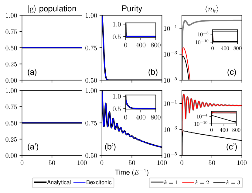
Consider first the case in which and . In this case the dynamics is pure-dephasing as , and independent of as there is no relaxation. This limit of the dynamics admits an analytical solution [40, 2] that we now use to test the bexcitonic formalism in number representation [Eq. (14)]. Figure 2 shows the dynamics of the (a-a’) population of , (b-b’) the qubit purity and (c-c’) the -bexciton population. The top panels (a-c) are for the DL bath while the bottom panels (a’-c’) for the Brownian bath. As shown, the bexcitonics exactly reproduces the analytical results. In the DL case, the purity decays monotonically as expected for a system interacting with a macroscopic environment and settles at which corresponds to the maximally mixed state. By contrast for the Brownian environment the purity exhibits an oscillatory dynamics before decay to . These oscillations are due to changes in system–bath entanglement as the Brownian environment oscillates. The purity asymptotically stays at as there are no relaxation process at play.
With respect to the bexcitons, initially, the -bexciton population is . Upon time evolution the population of all three considered bexcitons initially increases as system-bath interact. For DL, the bexciton is the high-temperature term in Eq. (6) and are the low temperature corrections. For Brownian and are the high-temperature terms and is a low temperature correction. For Brownian, there is a population degeneracy of the () bexcitons needed to describe .
In this pure-dephasing case, the high-temperature bexcitons reach steady state with non-zero at the long-time limit. By contrast, the low temperature correction terms go to zero after the initial excitation. The time required for the bexciton population to reach the steady state coincides with the time needed for the system to reach the maximally mixed state with . Therefore, the bexciton population reflects the entanglement between the system and the bath. The non-zero bexciton population at the final steady state reflects the non-separable system-bath state at equilibrium.
III.2 Relaxation dynamics of biased () qubit
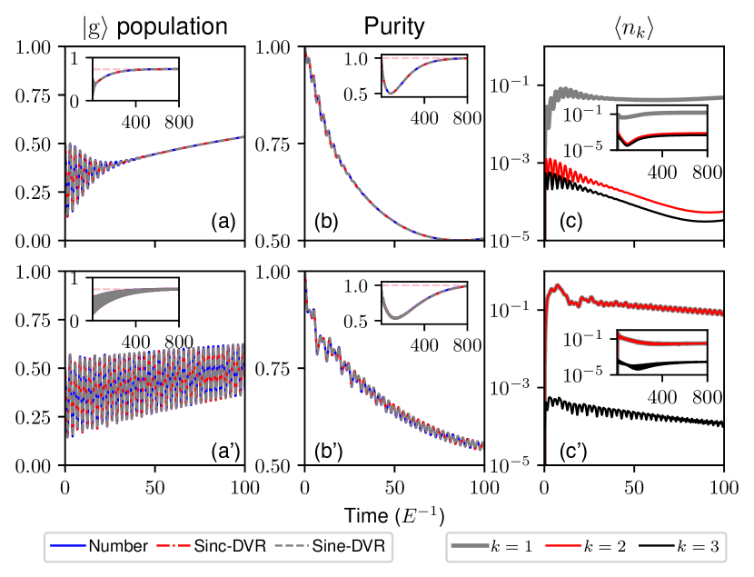
Figure 3 shows the dynamics of the qubit model beyond the pure-dephasing limit with . This is referred to the biased system case as [54]. In this case, the dephasing is accompanied by relaxation processes. The parameters of the model correspond to a complex case where the dynamics of the system and environment do not have a clear separation of time scales. The top panels (a-c) are for the DL bath while the bottom panels (a’-c’) for the Brownian bath. In both cases, the population of exhibits Rabi oscillations that decay due to decoherence. This process leads to a reduction of purity to a maximally mixed state (). At longer time scales, there is a recovery of purity as the system thermally relaxes to the ground state (insets). The dynamics correctly captures both the early time dynamics [55] and the asymptotic thermal state, and is representative of what is expected of open quantum dynamics. Note that different representations (position and number) lead to identical system dynamics, as expected from Eq. (12).
With respect to the bexcitonics, for both DL and Brownian bath, the relative bexciton populations indicate that the high-temperature bexciton dominates the dynamics. However, the low-temperature bexcitons are still required to achieve correct thermalization. The fact that the bexciton population is non-zero reflects that the system-bath state is not separable at thermal equilibrium.
Changing representations can vastly change the convergence properties of Eq. (12) but leaves bexcitonic properties invariant. We find that the number representation is often more efficient as it employs the exact eigenstates . Changing the metric changes both the convergence and bexcitonic properties of Eq. (12), and can be used to develop optimal EQMEs. The relative bexcitonic populations (but not their absolute values) are indicative of the importance of a given bexciton during the dynamics and can be used to test the completeness of Eq. (6) and the numerical convergence of Eq. (12).
III.3 Relaxation dynamics of unbiased () qubit

Figure 4 shows the dynamics for the qubit with and . This is referred as the unbiased system case [54]. The top panels (a-c) are for the DL bath while the bottom panels (a’-c’) for the Brownian bath. In this case, the population for is fixed at , as the rate of population exchange equals to the rate . However, the overall purity dynamics shows similar behavior as in the biased case in Fig. 3. That is, the decoherence process leads to a reduction of purity to a maximally mixed state first, and at longer time scales, there is a recovery of purity as the system thermally relaxes and re-purifies to a global steady state. For the unbiased system we observe that the dynamics of bexcitons shows similar trend as in the biased system for the longer time scale dynamics.
IV Conclusion
In conclusion, we have isolated a class of exact master equations for the open quantum dynamics of systems in interaction with bosonic thermal environments of arbitrary complexity. This dynamics is exactly captured by that of the quantum system interacting with a few bexcitons, fictitious bosonic quasiparticles each one arising from a distinct feature of the bath correlation function. The approach provides a systematic strategy to develop exact quantum master equations and captures variants of the HEOM as specific examples. While bexcitonic properties are unphysical, they can be used to monitor numerical convergence and guide the development of convenient and computationally efficient exact quantum master equations.
Acknowledgements.
This work was supported by a PumpPrimer II award of the University of Rochester and, partially, by the National Science Foundation under Grant Nos. CHE-2102386 and PHY-2310657. Computing resources are provided by the Center for Integrated Research Computing at the University of Rochester. The authors thank Gabriel Landi and Oliver Kühn for very helpful discussions on the subject.Appendix A Derivation of the bexcitonic exact quantum master equation Eqs. (12) and (13)
To capture the open quantum dynamics exactly, we need to take into account how each in Eq. (9) influences the system’s dynamics. The master equation is derived by taking the time-derivative of Eq. (10) as
| (19) |
Note that the derivatives of the bexciton generator are
| (20) |
Here we have used Eq. (4) and
| (21) |
Using these results, each term in the first sum in Eq. (19) becomes
| (22) |
for . Using Eq. (2), the last part in Eq. (19) can be expressed as
| (23) |
Hence,
| (24) |
where we have used the fact that
| (25) |
and
| (26) |
for . From Eqs. (19), (22) and (24),
| (27) |
Thus, to capture the exact open quantum dynamics it is necessary to follow the dynamics of all auxiliary density matrices that define the EDO.
We define an extended density operator (EDO) as a collection of these auxiliary density matrices. We arrange these matrices as a vector of matrices in a basis such that . The physical system’s density matrix corresponds to . In this space, we can define the creation and annihilation operators associated to the -th feature of the bath such that
| (28) |
and , . We define a metric operator for the -bexciton as . Hence,
| (29) | ||||
| (30) |
and
| (31) |
Inserting Eqs. (29), (30) and (31) into Eq. (27), we obtain
| (32) |
Since the the equation must be valid for arbitrary , then
| (33) |
To obtain the final EQME we only need to express Eq. (33) in the Schrödinger picture. Since the interaction picture is only for the physical system, and not for the introduced bexcitons, the procedure just requires changing the system operators to the Schrödinger and recovering the systematic dynamics due to the system’s Hamiltonian. In the Schrödinger picture,
| (34) |
where
| (35) |
are the dissipators in the dynamics. This yields Eqs. (12) and (13) in the main text.
References
- Breuer and Petruccione [2002] H. P. Breuer and F. Petruccione, The Theory of Open Quantum Systems (Oxford University Press, 2002).
- Schlosshauer [2007] M. Schlosshauer, Decoherence and the Quantum-To-Classical Transition (Springer-Verlag GmbH, 2007).
- Nielsen and Chuang [2011] M. A. Nielsen and I. L. Chuang, Quantum Computation and Quantum Information (Cambridge University Press, 2011).
- May and Kühn [2011] V. May and O. Kühn, Charge and Energy Transfer Dynamics in Molecular Systems (Wiley VCH Verlag GmbH, 2011).
- Tanimura [2020] Y. Tanimura, J. Chem. Phys. 153, 20901 (2020).
- Cygorek et al. [2022] M. Cygorek, M. Cosacchi, A. Vagov, V. M. Axt, B. W. Lovett, J. Keeling, and E. M. Gauger, Nat. Phys. 18, 662 (2022).
- Landi et al. [2022] G. T. Landi, D. Poletti, and G. Schaller, Rev. Mod. Phys. 94, 045006 (2022).
- Popp et al. [2019] W. Popp, M. Polkehn, R. Binder, and I. Burghardt, J. Phys. Chem. Lett. 10, 3326 (2019).
- Cao et al. [2020] J. Cao, R. J. Cogdell, D. F. Coker, H.-G. Duan, J. Hauer, U. Kleinekathofer, T. L. C. Jansen, T. Mancal, R. J. D. Miller, J. P. Ogilvie, V. I. Prokhorenko, T. Renger, H.-S. Tan, R. Tempelaar, M. Thorwart, E. Thyrhaug, S. Westenhoff, and D. Zigmantas, Sci. Adv. 6, eaaz4888 (2020).
- Koch [2016] C. P. Koch, J. Phys. Condens. Matter 28, 213001 (2016).
- Koch et al. [2022] C. P. Koch, U. Boscain, T. Calarco, G. Dirr, S. Filipp, S. J. Glaser, R. Kosloff, S. Montangero, T. Schulte-Herbrüggen, D. Sugny, and F. K. Wilhelm, EPJ Quantum Technol. 9, 19 (2022).
- Tanimura [1990] Y. Tanimura, Phys. Rev. A 41, 6676 (1990).
- Makri and Makarov [1995a] N. Makri and D. E. Makarov, J. Chem. Phys. 102, 4600 (1995a).
- Makri and Makarov [1995b] N. Makri and D. E. Makarov, J. Chem. Phys. 102, 4611 (1995b).
- de Vega et al. [2015] I. de Vega, U. Schollwock, and F. A. Wolf, Phys. Rev. B 92, 155126 (2015).
- Strathearn et al. [2018] A. Strathearn, P. Kirton, D. Kilda, J. Keeling, and B. W. Lovett, Nat. Commun. 9, 3322 (2018).
- Lambert et al. [2019] N. Lambert, S. Ahmed, M. Cirio, and F. Nori, Nat. Commun. 10, 3721 (2019).
- Tamascelli et al. [2019] D. Tamascelli, A. Smirne, J. Lim, S. F. Huelga, and M. B. Plenio, Phys. Rev. Lett. 123, 090402 (2019).
- Kim and Franco [2021] C. W. Kim and I. Franco, J. Chem. Phys. 154 (2021).
- Feynman and Vernon [1963] R. P. Feynman and F. L. Vernon, Ann. Phys. 24, 118 (1963).
- Caldeira and Leggett [1983] A. O. Caldeira and A. J. Leggett, Ann. Phys. 149, 374 (1983).
- Caldeira et al. [1993] A. O. Caldeira, A. H. CastroNeto, and T. O. de Carvalho, Phys. Rev. B 48, 13974 (1993).
- Suárez and Silbey [1991] A. Suárez and R. Silbey, J. Chem. Phys, 95, 9115 (1991).
- Tanimura and Kubo [1989] Y. Tanimura and R. Kubo, J. Phys. Soc. Jpn. 58, 101 (1989).
- Shi et al. [2009] Q. Shi, L. Chen, G. Nan, R.-X. Xu, and Y. Yan, J. Chem. Phys. 130, 84105 (2009).
- Ishizaki and Fleming [2009] A. Ishizaki and G. R. Fleming, J. Chem. Phys. 130, 234111 (2009).
- Ikeda and Scholes [2020] T. Ikeda and G. D. Scholes, J. Chem. Phys. 152, 204101 (2020).
- Anto-Sztrikacs et al. [2023] N. Anto-Sztrikacs, A. Nazir, and D. Segal, PRX Quantum 4, 020307 (2023).
- Somoza et al. [2019] A. D. Somoza, O. Marty, J. Lim, S. F. Huelga, and M. B. Plenio, Phys. Rev. Lett. 123, 100502 (2019).
- Lindblad [1976] G. Lindblad, Communications in Mathematical Physics 48, 119 (1976).
- Redfield [1965] A. G. Redfield, in Advances in Magnetic Resonance, Advances in Magnetic and Optical Resonance, Vol. 1 (Academic Press, 1965) pp. 1–32.
- Lidar [2019] D. A. Lidar, ArXiv e-prints , 1902.00967 (2019).
- Callen and Welton [1951] H. B. Callen and T. A. Welton, Phys. Rev. 83, 34 (1951).
- Hu et al. [2010] J. Hu, R.-X. Xu, and Y. Yan, J. Chem. Phys. 133, 101106 (2010).
- Zheng et al. [2009] X. Zheng, J. Jin, S. Welack, M. Luo, and Y. Yan, J. Chem. Phys, 130, 164708 (2009).
- Cui et al. [2019] L. Cui, H.-D. Zhang, X. Zheng, R.-X. Xu, and Y. Yan, J. Chem. Phys, 151, 10.1063/1.5096945 (2019).
- Zhang et al. [2020] H.-D. Zhang, L. Cui, H. Gong, R.-X. Xu, X. Zheng, and Y. Yan, J. Chem. Phys, 152, 064107 (2020).
- Xu et al. [2022] M. Xu, Y. Yan, Q. Shi, J. Ankerhold, and J. T. Stockburger, Phys. Rev. Lett. 129, 230601 (2022).
- Mukamel [1995] S. Mukamel, Principles of Nonlinear Optical Spectroscopy, Oxford series in optical and imaging sciences (Oxford University Press, 1995).
- Gustin et al. [2023] I. Gustin, C. W. Kim, D. W. McCamant, and I. Franco, Proceedings of the National Academy of Sciences 120, 10.1073/pnas.2309987120 (2023).
- Kim et al. [2022] C. W. Kim, J. M. Nichol, A. N. Jordan, and I. Franco, PRX Quantum 3, 040308 (2022).
- Caldeira and Leggett [1981] A. O. Caldeira and A. J. Leggett, Phys. Rev. Lett. 46, 211 (1981).
- Grabert et al. [1988] H. Grabert, P. Schramm, and G.-L. Ingold, Phys. Rep. 168, 115 (1988).
- Garg et al. [1985] A. Garg, J. N. Onuchic, and V. Ambegaokar, J. Chem. Phys. 83, 4491 (1985).
- Liu et al. [2014] H. Liu, L. Zhu, S. Bai, and Q. Shi, J. Chem. Phys. 140, 134106 (2014).
- Ikeda and Nakayama [2022] T. Ikeda and A. Nakayama, J. Chem. Phys. 156, 104104 (2022).
- Tang et al. [2015] Z. Tang, X. Ouyang, Z. Gong, H. Wang, and J. Wu, J. Chem. Phys. 143, 224112 (2015).
- Xu et al. [2023] M. Xu, V. Vadimov, M. Krug, J. T. Stockburger, and J. Ankerhold, ArXiv e-prints (2023).
- Colbert and Miller [1992] D. T. Colbert and W. H. Miller, Molecular dynamics with electronic transitions J. Chem. Phys. 96, 1061 (1992).
- Harris et al. [1965] D. O. Harris, G. G. Engerholm, and W. D. Gwinn, J. Chem. Phys. 43, 1515 (1965).
- Littlejohn et al. [2002] R. G. Littlejohn, M. Cargo, T. Carrington, K. A. Mitchell, and B. Poirier, J. Chem. Phys, 116, 8691 (2002).
- Paszke et al. [2019] A. Paszke, S. Gross, F. Massa, A. Lerer, J. Bradbury, G. Chanan, T. Killeen, Z. Lin, N. Gimelshein, L. Antiga, A. Desmaison, A. Köpf, E. Yang, Z. DeVito, M. Raison, A. Tejani, S. Chilamkurthy, B. Steiner, L. Fang, J. Bai, and S. Chintala, ArXiv e-prints , 1912.01703 (2019).
- Note [1] X. Chen. BEX: A general python package to simulate open quantum systems. Available at https://github.com/vINyLogY/bex.
- Sayer and Montoya-Castillo [2023] T. Sayer and A. Montoya-Castillo, The Journal of Chemical Physics 158, 10.1063/5.0132614 (2023).
- Gu and Franco [2017] B. Gu and I. Franco, J. Phys. Chem. Lett. 8, 4289 (2017).