The Significance of Data Abstraction Methods in Machine Learning Classification Processes for Critical Decision-Making

Abstract

The applicability of widely adopted machine learning (ML) methods to classification is circumscribed by the imperatives of explicability and uncertainty, particularly evident in domains such as healthcare, behavioural sciences, and finances, wherein accountability assumes priority. Recently, Small and Incomplete Dataset Analyser (SaNDA) has been proposed to enhance the ability to perform classification in such domains, by developing a data abstraction protocol using a ROC curve-based method. This paper focuses on column-wise data transformations called abstractions, which are crucial for SaNDA’s classification process and explores alternative abstractions protocols, such as constant binning and quantiles. The best-performing methods have been compared against Random Forest as a baseline for explainable methods. The results suggests that SaNDA can be a viable substitute for Random Forest when data is incomplete, even with minimal missing values. It consistently maintains high accuracy even when half of the dataset is missing, unlike Random Forest which experiences a significant decline in accuracy under similar conditions.

Classification is characterised by the attributes of explicability and uncertainty management

Medical, behavioural and financial datasets, among others, are often small and full of missing data

SaNDA was proposed as an explainable method tweaked for such datasets

This paper analyses how different abstraction methods influence SaNDA’s performance

Modified SaNDA with new abstraction methods is compared against first version of SaNDA and Random Forest

1 Introduction

The recent upswing in the adoption and advancement of Artificial Intelligence (AI) applied to classification for Critical Decision-Making (CDM) has been propelled by the implementation of deep learning, grounded in the unique amalgamation of substantial datasets (big data) and the availability of computational power [20]. This adoption of deep learning is centred on the comparative analysis of outcomes between human decision-making and machine-driven processes. However, this prompts question on the degree of comparability between these outcomes [24].

Classification for CDM processes encompasses two fundamental attributes: explainability [24] and uncertainty [34], characteristics notably absent in outcomes generated by deep learning [6, 30]. The integration of deep learning into CDM processes has encountered obstacles due to its opaque nature [19, 12], leading to the emergence of research trends such as eXplainable Artificial Intelligence (XAI) [18, 27] and one-shot learning [17].

Explainability holds particular and pivotal significance in the technological assimilation within CDM, primarily due to accountability concerns [6]. When ML informs CDM, a comprehensive explanation is imperative to elucidate the classification rationale, facilitating a deeper understanding of the decision-making process.

Nowadays, among various ML methods, deep learning is commonly used, as it has a huge advantage in finding patterns in the data. However, the application of deep learning requires the collection of substantial datasets, which is not achievable in many areas. Presence of small and missing data, characteristic for many fields, causes uncertainty [30] to be an inherent property of CDM scenarios [28].

Despite the advancements on data access [25], federated learning [37] and encrypted learning techniques [33], these challenges persist among others across diverse domains, including healthcare, behavioural sciences, and finances [5, 8, 21]. Moreover, challenges such as privacy concerns, limited accessibility, ethical considerations, and inherent data nature impend the acquisition of significant datasets [26, 14, 35, 31]. Therefore, it is necessary to focus on creating solutions for small and incomplete data.

Random Forest was originally presented as an approach for improving the accuracy of single decision tree which sometimes has problem with over-fitting and therefore with generalisation [3]. Random Forest [4] is based on an ensemble of individual decision tree trained on random samples of the training data, thereby achieving different characteristics of the data distribution. Once the decision trees have been constructed, the random forest algorithm makes a prediction by averaging the predictions of all of the trees reducing the variance of the model. This produces more accurate predictions than any individual tree could make, while remaining explainable. Moreover, in case of medium size, tabular datasets, Random Forest may outperform deep learning on classification task [10, 11]. These two properties make them suitable for use in many sensitive areas.

However, similarly to the majority of the widely used ML algorithms, they are unable to properly proceed with missing values. Therefore, they require removal of incomplete entries, or, when it is not possible or undesired, filling them with the help of imputation.

An alternative explainable ML method, SaNDA, built on the use of incomplete data and with the classification explainability provided by knowledge graphs (KG), has been recently proposed by us [15]. The solution eliminates the need for imputers, which can introduce erroneous information into the model, especially when the number of missing values is high or there is a bias in their occurrence. In addition to KG, another important element of SaNDA are abstractions, which is the transformation of data values into a smaller categorical distribution. More specifically, for each column of data, SaNDA assigns the values it contains to one of two states (categories) called $UP$ or $DOWN$. However, this binary abstraction choice is not the only possible one. This paper investigates the impact of other abstraction methods on the classification performance of SaNDA. The aim of the experiments is to improve SaNDA’s performance in classification processes for CDM, while maintaining functionality, even with very large amounts of missing data.

Sec. 2 provides a more detailed description of the classification process of SaNDA, as well as the alternative abstraction methods proposed in this paper and the metrics used to evaluate model performance. Research questions and descriptions of the experiments undertaken to answer them are described in Sec. 3. Results of the numerical experiments are given in Sec. 4. Finally, the paper is closed with a summary and conclusions (Sec. 5).

2 Model

2.1 Verification metrics

Several metrics are used as a valuable tool for comparing the performance of ML classification models. They provide a comprehensive assessment of a model’s performance across different aspects. To define chosen metrics the following basic concepts as results of the classification task should be introduced:

• True positives ($\mathrm{TP}$) - number of correctly classified instances of the positive class,

• False positives ($\mathrm{FP}$) - number of incorrectly classified instances of the negative class,

• True negatives ($\mathrm{TN}$) - number of correctly classified instances of the negative class,

• False negatives ($\mathrm{FN}$) - number of incorrectly classified instances of the positive class.

Based on the concepts several metrics of classification tasks are defined. Among these, balanced accuracy (BA) provides a comprehensive assessment of model performance. BA is the primary metrics chosen for evaluation the performance of selected abstraction methods and comparing them with Random Forest. It is one of the simplest metrics for evaluating a classification model’s ability to accurately predict classes in the context of imbalanced datasets, which are common, among others, for medical and financial problems. BA is a extension of standard accuracy metrics, it is an average accuracy from both the minority and majority classes, i.e.,

$$\mathrm{BA}=\frac{\frac{\mathrm{TP}}{\mathrm{TP}+\mathrm{FN}}+\frac{\mathrm{TN}}{\mathrm{TN}+\mathrm{FP}}}{2}.$$ (1)

Beyond a simple BA, there are other metrics which offer different insights into how well a classification model is performing [13]. Recall, defined as

$$\mathrm{recall}=\frac{\mathrm{TP}}{\mathrm{TP}+\mathrm{FN}},$$ (2)

measures the ability for the correct identification of instances of the positive class from all the actual positive samples in the dataset. This metrics is widely employed in various domains, particularly in application classification algorithms used, e.g. in medical and financial scenarios. For instance, in healthcare it is crucial especially in medical screening and diagnostic testing as high value of recall suggests that the test performs well in detecting $\mathrm{TP}$ cases, thereby reducing the chances of missing instances ($\mathrm{FN}$) [13]. In financial area, recall is frequently measured in the context of risk management and fraud detection to ensure that potential risks or fraudulent activities are detected effectively [22].

However, there are also scenarios, where the accuracy of positive predictions made by a classification model is critical, e.g. consequences of carrying out medical or financial interventions or procedures that are not actually required, stemming from false positive results, can have a substantial impact. In such case precision should be monitored. Precision provides information about the quality of positive predictions made by the model. It is defined as the number of positive instances divided by the total number of positive predictions, both correctly and incorrectly classified as positive class:

$$\mathrm{precision}=\frac{\mathrm{TP}}{\mathrm{TP}+\mathrm{FP}}$$ (3)

Achieving a careful equilibrium between recall and precision holds paramount importance in many applications. However, the optimal metrics for evaluation ML models should be chosen based on the specific scope and nature of the problem at hand.

2.2 SaNDA classification method

SaNDA consists of two main parts, which interacts with each other to provide comprehensive method of data analysis: classification, and KG [15]. While classification module can separate data into classes and provide information how well model captures properties of the data, KG enhance explainability of the results and provide deeper insight into interdependence between features. Since the primary objective of this paper is to investigate the potential for enhancing SaNDA’s data representation capability, which is primarily evaluated through the classification aspect, this section focuses on the explanation of classification method using SaNDA. The most important concepts for a classification problem using SaNDA are abstractions and the classification algorithm itself.

Data abstraction involves simplifying a specific set of data by condensing it into a more streamlined representation of the entire dataset. It allows for eliminating specific traits from an object or concept to distill it down to a collection of fundamental elements. To this end, data abstraction creates a simplified representation of the underlying data, while hiding its complexities and associated operations. In addition, abstraction method used in SaNDA ensures the anonymisation of the data. There are various approaches to creating abstractions.

The abstraction is formally defined as [15]:

Definition 1.

Given $A$ and $B$ two sets of numerical values, with $|A|\geq|B|$, an abstraction is defined as a function $\mathcal{F}:A\to B$ that maps the values of $A$ to values of $B$.

In other world, process of abstraction maps original values from the data into smaller set of values. It is important to mention that abstraction process is performed on column-by-column basis. In the founding paper, original data was transformed into two classes, using ROC curve method. However, other methods resulting in the different number of abstractions (categories), i.e., cardinality of set $|B|\neq 2$, may also be an appropriate solution. All of the methods using ROC curves and the new proposed alternative methods are presented in the subsection 2.3. For the need of SaNDA, elements of the new set are represent as $B={B_{1},...,B_{|B|}}$ and can be treated as a set of categorical variables. Therefore, if every of $n$ features in the dataset is abstracted to the same amount of abstractions, each input is now described by a set of categorical values $X=\{x_{1},\cdots,x_{n}\}$. The input constructed in this way can be combined with the natively categorical data, enabling easy integration of different types of data [9].

Then based on obtained data abstractions, we generate an explainable KG representation, which is created as it was previously described [16, 15]. Through building the graphs, a representation for each class based on available features is prepared. The significance of each vertex of the KG is represented by the probability of each feature being in given category of the given class.

Following paper focuses on binary classification, however SaNDA algorithm can be described and performed also for arbitrary number of classes [9, 15]. Let $C_{j}$ be the $j$th class. Then for given $C_{j}$ the following probability can be computed as:

$$P(X|C_{j})=\prod_{i=1}^{n}P(x_{i}|C_{j})$$ (4)

The class with the highest $P(X|C_{j})$ is chosen, i.e.

$$\mathrm{argmax}_{C}\left\{P(X|C_{j})\right\}.$$ (5)

Therefore, SaNDA assigns a given set of values to the class for which its occurrence is most likely. If the given feature $x_{i}$ is empty (missing value) or is represented by null values, it is skipped in the calculation of the probability $P(X|C_{j})$.

Contrary to the majority of commonly used methods, SaNDA does not divide feature space base on optimisation of some classification function. Instead values of every feature are individually divided based on abstraction methods, which does not need (but can) take into account class distribution. From the perspective of the entire feature space, it creates division into grind, which every “cell” is label as one of the classes based on the conditions given by Eqs. (4) and (5). These conditions do not consider every individual “cell” but rather try to approximate it base on every dimension separately. On the one hand, this approach may diminish the classification accuracy of the method by failing to incorporate more intricate, nonlinear relationships, particularly in the context of a sparse grid (where the number of abstractions is low). On the other hand it allows to complete classification test even in the present of missing values by considering lower-dimensional space.

2.3 Abstraction methods

Abstraction as a procedure for reducing the number of values that a variable can take is defined in Sec. 2.2. This section presents methods of abstracting data used in this paper.

2.3.1 ROC Curves

ROC curve abstractions split the values of a feature into two categories in a way that maximizes the separation between the classes in the feature. To be more precise, the values of the feature in the abstracted column are split into smaller and larger than the value that maximizes BA, as given by Eq (1).

2.3.2 constant binning

Abstractions though constant binning divide the values of a feature into categories of equal range. Let $A$ be a set of the values taken by the feature. Then $L=\mathrm{max}A-\mathrm{min}A$ is a range of values. constant binning divide range of the data $L$, into $n$ equal intervals of length $L/n$, assigning the feature a number corresponding to the bin number in which its original value falls.

2.3.3 Quantiles

While constant binning divides data to keep the range of every bin equal, abstractions based on quantiles divide data into categories of the equal size. Cut-off values are chosen based on the values of quantiles. Quantile of the order $n$ is defined based on the probability distribution of the random variable ranging over the set $X$ is such a way that the locations $y_{q}$ of the quantile $q$ ($q=k/n$, where $k\leq n$) given by

$$q=\int_{-\infty}^{y_{q}}p(x)dx.$$ (6)

In other words, quantile $y_{q}$ is such value that cumulative distribution function takes at this point value $q$ or alternatively $q$th part of the data takes values smaller or equal $y_{q}$. Quantile-based abstractions therefore assign the feature the largest $k$ for which $x<y_{q}$, i.e., corresponding to the highest quantile larger than initial value.

The most commonly used quantiles are ones of the order $n=2$ (median), $n=4$ (quartiles) and $n=10$ (deciles).

3 Experiments

The main goal of this research is to improve the efficacy of the SaNDA algorithm by examining the abstraction phase. To achieve this, it is necessary to first explore how different abstraction methods influence the metrics that describe SaNDA performance. Based on the results, determine whether there are criteria for choosing an abstraction method that can be applied in model design, and if so, how to choose the best abstraction method for a given use of the SaNDA algorithm. Finally, verify how the best-performing abstraction methods influences SaNDA performance in the presence of missing values in the dataset. For the sake of comparison with the original research, we used the $5$ datasets from the paper proposing SaNDA [15] in the following experiments, supplemented by $10$ synthetic DIGEN datasets (8_4426, 10_8322, 17_6949, 22_2433, 23_5191, 24_2433, 32_5191, 35_4426, 36_466, 39_5578). A selection of datasets is briefly described below.

The Ionosphere dataset [7, 32], a collection of $351$ radar measures of the ionosphere in Goose Bay, Labrador, is used to classify its structure. The dataset includes $34$ numeric features that measure the number of free electrons and other electromagnetic signals in the ionosphere.

The Sonar dataset [7, 1] consists of $60$ numerical features that measure the shape and characteristics of the sonar signal. The classification task is to distinguish underwater surfaces as rock or metal. It is the smallest number of records equal to $208$.

The Wisconsin Breast Cancer dataset [7, 36] uses $30$ numerical features that measure the shape and composition of a breast mass to describe 569 fine needle aspirates. The task is to distinguish between cancerous and non-cancerous samples. It consists of $569$ entries.

The Accelerometer dataset [7, 29] was generated for prediction of motor failure time with application of an artificial neural network. It uses $4$ numerical features; $3$ of them represents the values of x, y and z axes, while the fourth is cooler maximum speed percentage ranging from $20$% to $100$% with $5$% intervals. The fifth attribute was used as target class, where normal configuration was admitted as negative class, while perpendicular and opposite configuration as positive class. It has the largest number of records equal to $102000$.

The HIGGS dataset [7, 2] is produced from Monte Carlo simulations of particle decays and contains $1.1\times 10^{7}$ entrances. Each process is described by $28$ features, of which $21$ are kinematic properties measured by the particle detectors in the accelerator and the remaining $7$ are quantities derived from them. The classification task is to distinguish between measurements of background noise and those connected to the observation of the Higgs particle. $10^{5}$ randomly selected records were taken for the experiments presented in this work.

DIGEN [23] datasets were designed to differentiate the performance of some of the leading classification methods. It is the collection of $40$ synthetic datasets created from each of the generative mathematical functions for testing binary classification task. Every dataset from DIGEN contains $10$ features of $1000$ normally distributed values.

In summary, the experimental setup consists of 13 small and 2 medium datasets. This disproportion is caused by the target domain for SaNDA, which is related to the nature of data occurring in personal health care or finances.

To achieve the goals of this research, we conducted two numerical experiments using the datasets described above. The first experiment focuses on exploring the different abstraction methods presented in the Sec 2.3 and their impact on SaNDA performance with an indication of classifciation accuracy. For this purpose, each of the studied datasets was transformed using one of the following abstraction methods:

• constant binning into 10 and 20 bins

• quantiles of order 10 (deciles) and 20

• using ROC curve method as a control group

Then, using the method used in SaNDA, models were created for classification purposes. It is important to note that in this experiment we do not create any missing data in the datasets.

Following the initial experiment, the abstraction methods yielding the highest BA was selected for each dataset with the selected percentage of missing data. Subsequently, the SaNDA classification algorithm was modified to incorporate this chosen abstraction methods and applied to datasets containing $1\%$, $5\%$, 10$\%$, and $50\%$ of missing data. Datasets with $n\%$ missing data were created from the original datasets by randomly removing $n\%$ of data from each column (feature). The results were compared to those obtained from the original, ROC curve-based SaNDA and Random Forest algorithms. For Random Forest, missing data were replaced with zeros to be able to process the datasets. Subsequently, for all of the methods the BA, recall and precision values were compared.

4 Results

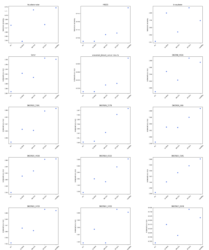
Figure 1: Balanced accuracy (BA) of SaNDA classification method as a function the different abstraction methods.

Figure 1 and Table 1 show the BA for experiment 1. For each dataset detailed in Section 3, it contrasts the BA acquired from SaNDA across various abstraction types: ROC, deciles (quantiles $10$), quantiles $20$, $10$ bins, and $20$ bins. For the accelerometer, Higgs, WDBC, and DIGEN datasets, with the exception of DIGENs: 22_2433, 24_2433, and 17_6949, the use of quantiles $20$ results in superior BA for classification. On the other hand, for the remaining DIGENs, Sonar and Ionosphere datasets, the application of $20$ bins abstraction yields higher BA compared to other abstraction methods.

Based on this experiment, it can be observed that overall quantiles $20$ offers better classification performance compared to $20$ bins abstraction method. In the case of the opposite being true, the discrepancy is significantly narrower. Similar but weaker trend can be also observed between deciles and $10$ bins. In light of the results, quantile-based abstractions can be regarded as a preferable choice of abstraction for SaNDA classification.

However, the number of categories into which data is transformed as a result of abstraction process is of far greater significance than the type of abstraction employed. This can be explained by the fact that a higher number of abstractions (categories) enhances the resolution of the grid created in the feature space. As a result, a denser grid enables a more homogeneous distribution of data across its constituent parts, leading to more accurate classification performance.

One might naively believe that increasing the number of abstractions will enhance classification accuracy. However, this approach harbours potential pitfalls that warrant careful consideration. First, increasing the number of abstractions can result in a decrease in the average number of data points per category, potentially compromising the accurate representation of statistical properties. Furthermore, an increase in the number of abstractions can lead to an expansion in the number of nodes within the KG generated by SaNDA, potentially diminishing its explainability. Finally, an extensive number of abstractions can exert a detrimental impact on the computational time required for generating classification and KG, a factor that may become particularly crucial when computational resources are constrained or the analysed problem demands expediency. Given these considerations, the maximum number of abstractions employed in this research was limited to 20.

Based on the results of Experiment 1, Experiment 2 employed SaNDA classification using $20$ bins and quantiles $20$ for comparison with the original ROC curves abstractions and Random Forest was performed. The results of this comparison for increasing percentage of missing data are presented in Figs 2–4 and in Tables 1–15. Fig. 2 shows BA as a function of missing data for each dataset separately. In all of the cases, 20 categories abstractions, bin- or quantile-based, outperform both ROC-based abstractions. Random Forest achieves higher BA in only $4$ of $15$ datasets with non-zero amount of missing data: Accelerometer, HIGGS and DIGENs: 39_5578, 23_5191. However, for HIGGS and DIGEN23_5191 the difference between $20$ quantiles abstractions SaNDA and Random Forest in the BA is slight. When the proportion of missing data increases the advantage of SaNDA with 20 categories abstraction methods increases, as it achieves higher BA for majority of tested datasets. A notable exception is observed in the Accelerometer dataset, where Random Forest surpasses both proposed new abstraction methods regardless of amount of missing values. This behaviour can be attributed to the limited number of features, specifically $4$, characterising this dataset. Additionally, the size of the dataset, which can be considered average with approximately $10^{5}$ inputs, favors the efficiency of Random Forest.

BA is not the only important metrics from the point of view of classification models. The proposed system, due to its ability to anonymize data and dealing with missing values may be particularly relevant, among others, in areas of medicine, social sciences and finance where the high level of recall and precision is also very important. Therefore, we decided to check whether increasing the number of abstractions (categories) would affect mentioned metrics and compare them with the values obtained for Random Forest. The results presented in Figure 3 showed that the recall was higher for quantiles $20$ than for ROC for all of the chosen datasets. Comparison of quantiles $20$ and Random Forest shows that Random Forest wins in the case of 6 datasets (Accelerometer, HIGGS, Wisconsin Breast Cancer and DIGENs: 8_4426, 39_5578, 23_5191, when there aren’t any missing values. Quantiles $20$ or $20$ bins achieves better results for $9$ datasets (Ionosphere, Sonar and DIGENs: 32_5191, 36_466, 35_4426, 10_8322, 22_2433, 24_2433, 17_6949) with an advantage for quantiles. The only dataset where Random Forest performance is much better is Accelerometer, but the same observation was noticed for BA and it may be related to low number of features.

Similar conclusions were reached for precision, see Fig. 4. For all datasets, the proposed new abstraction methods performed significantly better than ROC. In the absence of missing data Random Forest achieves highest precision values for $6$ (HIGGS, Ionosphere, Wisconsin Breast Cancer and DIGENs: 39_5578, 23_5191, 22_2433) of $15$ datasets, in the case of $2$ of these datasets the difference was marginal (DIGENs: 23_5191 and 22_2433). For the rest of the datasets, classification using either quantiles $20$ or $20$ bins yields higher precision (Accelerometer, Sonar and DIGENs: 8_442, 32_5191, 36_466, 35_4426, 10_8322, 24_2433, 17_6949). With $10$% of the missing data quantiles $20$ or $20$ bins outperform Random Forest in $12$ out of $15$ cases for recall (HIGGS, Ionosphere, Sonar and DIGENs: 8_442, 32_5191, 39_5578, 36_466, 35_4426, 10_8322, 23_5191, 24_2433, 17_6949) and in $12$ cases for precision (Accelerometer, HIGGS, Sonar and DIGENs: 32_5191, 39_5578, 36_466, 35_4426, 10_8322, 23_5191, 24_2433, 17_6949). A greater proportion of missing data works against Random Forest, which is particularly noticeable when $50$% of data is removed - in such conditions Random Forest prevails by a minimal margin for only 1 dataset (for recall - Accelerometer, while for precision - DIGEN39_5578).

The results clearly demonstrate that the proposed new data abstraction methods significantly outperform abstractions using ROC. Moreover, the values obtained from selected metrics indicate that classification using SaNDA with a quantiles $20$ abstraction method can compete with Random Forest for complete datasets. Additionally, classification with missing data clearly shows the advantage of the new data abstraction methods over classical approach.

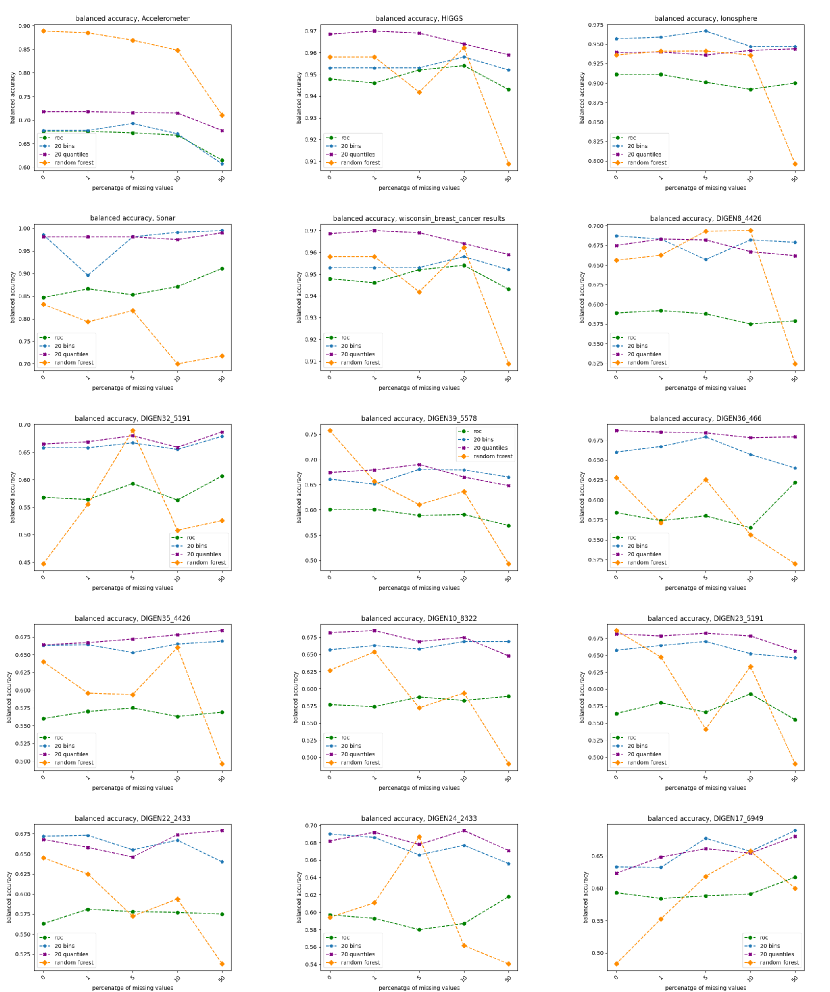
Figure 2: Balanced accuracy (BA) as a function of percentage of missing data for SaDNA with two best performing abstraction methods (order quantiles $20$ and $20$ bins), SaNDA with ROC curve and Random Forest.

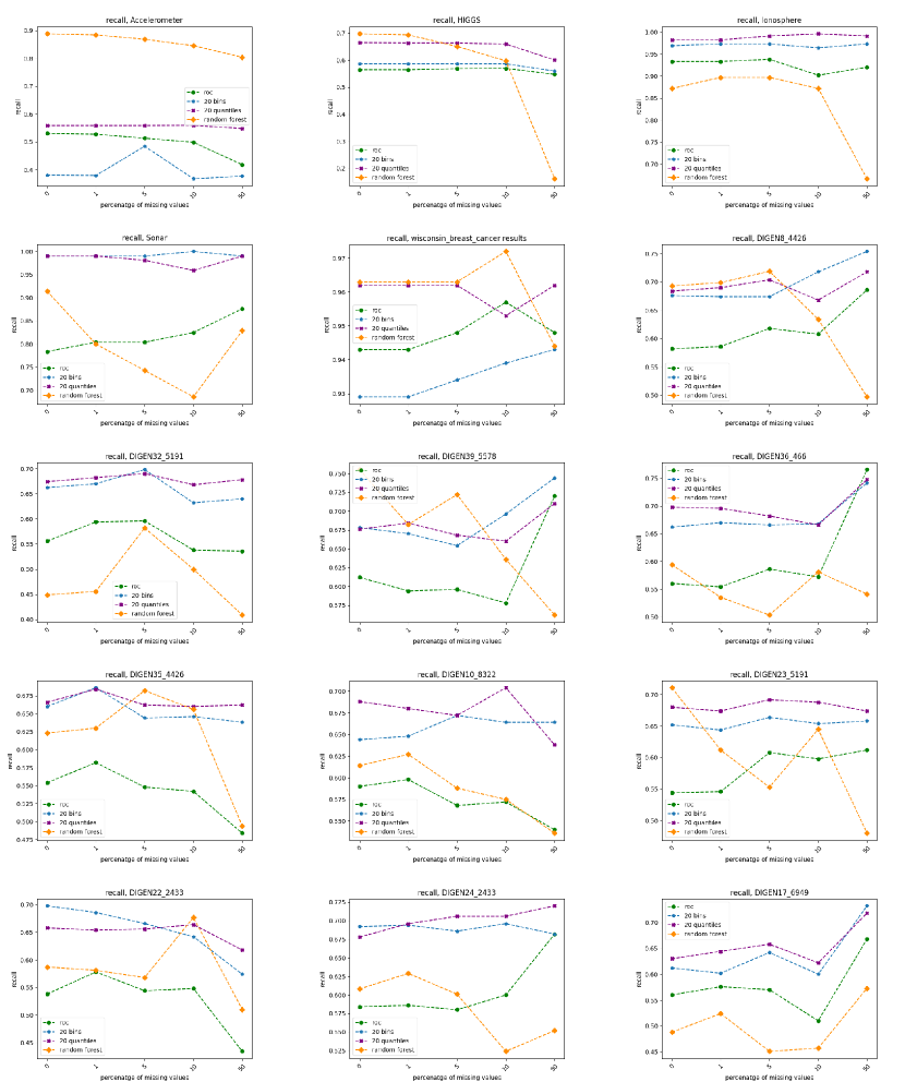
Figure 3: Recall as a function of percentage of missing data for SaDNA with two best performing abstraction methods (order quantiles $20$ and $20$ bins), SaNDA with ROC curve and Random Forest.

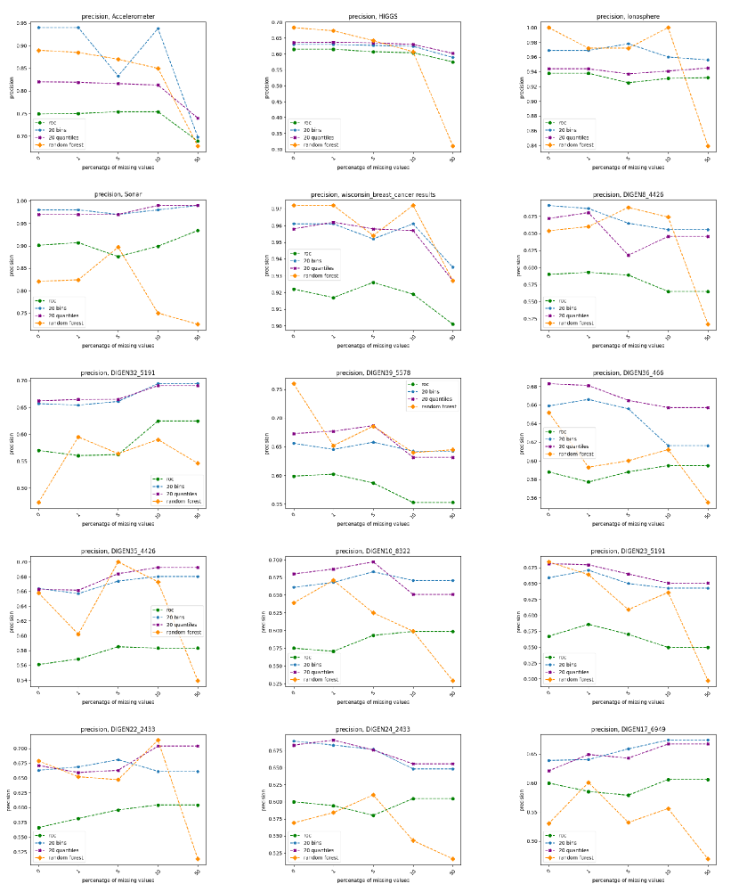
Figure 4: Precision as a function of percentage of missing data for SaDNA with two best performing abstraction methods (order quantiles $20$ and $20$ bins), SaNDA with ROC curve and Random Forest.

5 Summary and Conclusions

The increasing research on data anonymisation, federated learning and encrypted computing aims at increasing the data size and availability for deep learning, the driving force behind the recent developments and impact of ML. However, there are areas such as healthcare, behavioural sciences and finances, where data, to support CDM remains very limited. Recently, the Small and Incomplete Dataset Analyser (SaNDA) [15] has emerged as a promising solution to facilitate the adoption of ML in such areas due to its capability to use small and noisy datasets, while explaining the outcomes.

SaNDA can effectively tackle classification tasks even with substantial amounts of missing data, eliminating the need for data imputation or modelling, which can be challenging, costly and time-consuming in extremely low-quality datasets. One of its fundamental aspects is the use of abstractions, which involve column-wise transformations of numerical data into categorical representations.

In this paper we describe experiments to compare constant width constant binning and quantiles-based abstraction protocols as alternatives to the previously employed ROC curve-based method. Their influence on classification performance has been extensively examined and measured.

As a general result, increasing the number of data abstractions consistently enhances the performance of the SaNDA algorithm, however, this results into some potential limitations. Firstly, it was identified that splitting the data into many categories, results in a poor statistical representation of the real population. Secondly, it reduces the explainability of the model due to the increase of the complexity of the KG representation, becoming useless for Critical Decision-Making. Lastly, a substantial increase on the time required to create the classification model makes its usefulness questionable for the proposed classification environments.

Due to these limitations, we decided to cap the number of abstractions to $20$, regardless of the chosen abstraction method. This limit proved to be effective in significantly improving the balanced accuracy of SaNDA.

In conclusion, the SaNDA classification process, built through the meticulous experiments of a chosen abstraction methodology, holds as a prospective alternative to conventional explainable ML paradigms such as Random Forest. This assertion gains particular relevance in situations necessitating CDM within constraints of small datasets and missing data. The proposed SaNDA enhanced classification processes demonstrates its potential to yield robust and explainable outcomes, thereby presenting a viable option in contexts where deep learning methodologies may encounter limitations.

A future direction of research may involve the choice of an appropriate method and level of abstraction. The abstraction method can be chosen to maximise accuracy while maintaining computation time efficiency for a specific dataset. The abstraction level dictates how accurately it mirrors the intricacies of the problem domain and the extent to which it simplifies and generalizes domain concepts. It can range from being very detailed and specific to more generalized and fundamental, depending on the intended scope and purpose of the domain problems. Adopting a dynamic approach to selecting methods and determining abstraction levels can enhance the model’s versatility. This adaptability would allow for easy customization to meet specific problem and user requirements.

dataset	quantiles 20	deciles	ROC	10 bins	20 bins	Random Forest
DIGEN23_5191	0.681	0.633	0.564	0.601	0.657	0.686
DIGEN24_2433	0.682	0.597	0.597	0.635	0.690	0.594
DIGEN39_5578	0.674	0.622	0.601	0.603	0.661	0.757
DIGEN17_6949	0.623	0.602	0.593	0.615	0.633	0.483
DIGEN32_5191	0.665	0.602	0.568	0.605	0.658	0.447
DIGEN10_8322	0.682	0.611	0.577	0.620	0.657	0.627
DIGEN22_2433	0.668	0.603	0.563	0.611	0.672	0.645
DIGEN8_4426	0.675	0.623	0.589	0.648	0.687	0.656
DIGEN35_4426	0.664	0.627	0.560	0.611	0.663	0.640
DIGEN36_466	0.687	0.629	0.584	0.630	0.660	0.628
Accelerometer	0.718	0.713	0.676	0.638	0.678	0.889
Ionosphere	0.940	0.924	0.911	0.950	0.957	0.936
Wisconsin Breast Cancer	0.969	0.952	0.948	0.948	0.953	0.958
Sonar	0.981	0.906	0.847	0.923	0.986	0.832
HIGGS	0.663	0.658	0.624	0.609	0.640	0.666

Table 1: Balanced accuracy (BA) for selected SaNDA classification methods and Random Forest for all chosen datasets with $0\%$ missing values

dataset	quantiles 20	ROC	20 bins	Random Forest
DIGEN23_5191	0.678	0.58	0.664	0.647
DIGEN24_2433	0.692	0.593	0.686	0.611
DIGEN39_5578	0.679	0.601	0.651	0.657
DIGEN17_6949	0.648	0.584	0.632	0.553
DIGEN32_5191	0.669	0.564	0.658	0.555
DIGEN10_8322	0.685	0.574	0.663	0.654
DIGEN22_2433	0.658	0.581	0.673	0.625
DIGEN8_4426	0.683	0.592	0.683	0.663
DIGEN35_4426	0.667	0.57	0.664	0.596
DIGEN36_466	0.685	0.574	0.667	0.571
Accelerometer	0.718	0.676	0.678	0.885
Ionosphere	0.940	0.911	0.959	0.941
Wisconsin Breast Cancer	0.970	0.946	0.953	0.958
Sonar	0.981	0.866	0.896	0.793
HIGGS	0.663	0.624	0.639	0.661

Table 2: Balanced accuracy (BA) for selected SaNDA classification methods and Random Forest for all chosen datasets with $1\%$ missing values

dataset	quantiles 20	ROC	20 bins	Random Forest
DIGEN23_5191	0.682	0.566	0.670	0.541
DIGEN24_2433	0.678	0.580	0.666	0.687
DIGEN39_5578	0.690	0.589	0.680	0.610
DIGEN17_6949	0.661	0.588	0.677	0.618
DIGEN32_5191	0.680	0.593	0.667	0.689
DIGEN10_8322	0.669	0.588	0.658	0.572
DIGEN22_2433	0.646	0.578	0.655	0.572
DIGEN8_4426	0.682	0.588	0.657	0.693
DIGEN35_4426	0.672	0.575	0.653	0.594
DIGEN36_466	0.684	0.580	0.679	0.626
Accelerometer	0.716	0.673	0.693	0.869
Ionosphere	0.936	0.901	0.967	0.941
Wisconsin Breast Cancer	0.969	0.952	0.953	0.942
Sonar	0.981	0.853	0.981	0.818
HIGGS	0.661	0.620	0.637	0.614

Table 3: Balanced accuracy (BA) for selected SaNDA classification methods and Random Forest for all chosen datasets with $5\%$ missing values

dataset	20_deciles	roc	static_20	Random Forest
DIGEN23_5191	0.678	0.593	0.652	0.633
DIGEN24_2433	0.694	0.587	0.677	0.562
DIGEN39_5578	0.665	0.591	0.679	0.637
DIGEN17_6949	0.654	0.591	0.657	0.657
DIGEN32_5191	0.659	0.563	0.655	0.508
DIGEN10_8322	0.675	0.583	0.669	0.594
DIGEN22_2433	0.674	0.577	0.667	0.594
DIGEN8_4426	0.667	0.575	0.682	0.694
DIGEN35_4426	0.678	0.563	0.665	0.660
DIGEN36_466	0.678	0.565	0.657	0.556
Accelerometer	0.715	0.668	0.671	0.848
Ionosphere	0.942	0.892	0.947	0.936
Wisconsin Breast Cancer	0.964	0.954	0.958	0.962
Sonar	0.975	0.871	0.991	0.700
HIGGS	0.657	0.618	0.635	0.622

Table 4: Balanced accuracy (BA) for selected SaNDA classification methods and Random Forest for all chosen datasets with $10\%$ missing values

dataset	quantiles 20	ROC	20 bins	Random Forest
DIGEN23_5191	0.656	0.555	0.646	0.490
DIGEN24_2433	0.671	0.618	0.656	0.541
DIGEN39_5578	0.648	0.569	0.665	0.493
DIGEN17_6949	0.680	0.617	0.689	0.600
DIGEN32_5191	0.687	0.607	0.679	0.526
DIGEN10_8322	0.648	0.589	0.669	0.491
DIGEN22_2433	0.679	0.575	0.640	0.513
DIGEN8_4426	0.662	0.579	0.679	0.524
DIGEN35_4426	0.684	0.569	0.669	0.496
DIGEN36_466	0.679	0.622	0.640	0.520
Accelerometer	0.678	0.615	0.607	0.711
Ionosphere	0.944	0.900	0.947	0.796
Wisconsin Breast Cancer	0.959	0.943	0.952	0.909
Sonar	0.990	0.911	0.995	0.718
HIGGS	0.627	0.593	0.606	0.517

Table 5: Balanced accuracy (BA) for selected SaNDA classification methods and Random Forest for all chosen datasets with $50\%$ missing values

dataset	quantiles 20	ROC	20 bins	Random Forest
DIGEN23_5191	0.681	0.567	0.659	0.684
DIGEN24_2433	0.683	0.600	0.689	0.569
DIGEN39_5578	0.673	0.599	0.656	0.760
DIGEN17_6949	0.621	0.600	0.639	0.530
DIGEN32_5191	0.662	0.570	0.657	0.473
DIGEN10_8322	0.680	0.575	0.661	0.639
DIGEN22_2433	0.671	0.566	0.663	0.679
DIGEN8_4426	0.672	0.590	0.691	0.654
DIGEN35_4426	0.663	0.561	0.664	0.658
DIGEN36_466	0.683	0.588	0.659	0.652
Accelerometer	0.820	0.749	0.940	0.890
Ionosphere	0.944	0.938	0.969	1.000
Wisconsin Breast Cancer	0.958	0.922	0.961	0.972
Sonar	0.970	0.901	0.980	0.821
HIGGS	0.636	0.615	0.630	0.683

Table 6: Precision for selected SaNDA classification methods and Random Forest for all chosen datasets with $0\%$ missing values

dataset	quantiles 20	ROC	20 bins	Random Forest
DIGEN23_5191	0.679	0.586	0.671	0.664
DIGEN24_2433	0.690	0.594	0.683	0.584
DIGEN39_5578	0.677	0.602	0.645	0.652
DIGEN17_6949	0.649	0.585	0.640	0.601
DIGEN32_5191	0.665	0.560	0.654	0.595
DIGEN10_8322	0.687	0.571	0.668	0.671
DIGEN22_2433	0.659	0.581	0.669	0.652
DIGEN8_4426	0.680	0.593	0.686	0.660
DIGEN35_4426	0.662	0.568	0.657	0.602
DIGEN36_466	0.681	0.577	0.666	0.593
Accelerometer	0.819	0.750	0.940	0.885
Ionosphere	0.944	0.938	0.969	0.972
Wisconsin Breast Cancer	0.962	0.917	0.961	0.972
Sonar	0.970	0.907	0.980	0.824
HIGGS	0.637	0.615	0.630	0.673

Table 7: Precision for selected SaNDA classification methods and Random Forest for all chosen datasets with $1\%$ missing values

dataset	quantiles 20	ROC	20 bins	Random Forest
DIGEN23_5191	0.665	0.570	0.650	0.609
DIGEN24_2433	0.676	0.580	0.677	0.610
DIGEN39_5578	0.687	0.587	0.658	0.686
DIGEN17_6949	0.643	0.579	0.659	0.532
DIGEN32_5191	0.665	0.562	0.661	0.564
DIGEN10_8322	0.697	0.593	0.683	0.625
DIGEN22_2433	0.663	0.596	0.681	0.647
DIGEN8_4426	0.618	0.589	0.665	0.688
DIGEN35_4426	0.684	0.585	0.674	0.700
DIGEN36_466	0.665	0.588	0.656	0.600
Accelerometer	0.816	0.754	0.833	0.870
Ionosphere	0.937	0.925	0.978	0.972
Wisconsin Breast Cancer	0.958	0.926	0.952	0.954
Sonar	0.970	0.876	0.970	0.897
HIGGS	0.635	0.607	0.627	0.642

Table 8: Precision for selected SaNDA classification methods and Random Forest for all chosen datasets with $5\%$ missing values

dataset	quantiles 20	ROC	20 bins	Random Forest
DIGEN23_5191	0.651	0.549	0.643	0.497
DIGEN24_2433	0.656	0.605	0.648	0.516
DIGEN39_5578	0.632	0.553	0.642	0.645
DIGEN17_6949	0.667	0.606	0.674	0.469
DIGEN32_5191	0.690	0.625	0.694	0.546
DIGEN10_8322	0.651	0.599	0.671	0.529
DIGEN22_2433	0.704	0.604	0.661	0.513
DIGEN8_4426	0.646	0.565	0.656	0.517
DIGEN35_4426	0.692	0.583	0.680	0.539
DIGEN36_466	0.657	0.595	0.616	0.555
Accelerometer	0.740	0.689	0.698	0.678
Ionosphere	0.945	0.932	0.956	0.839
Wisconsin Breast Cancer	0.927	0.901	0.935	0.927
Sonar	0.990	0.934	0.990	0.725
HIGGS	0.602	0.575	0.589	0.310

Table 9: Precision for selected SaNDA classification methods and Random Forest for all chosen datasets with $10\%$ missing values

dataset	quantiles 20	ROC	20 bins	Random Forest
DIGEN23_5191	0.651	0.549	0.643	0.497
DIGEN24_2433	0.656	0.605	0.648	0.516
DIGEN39_5578	0.632	0.553	0.642	0.645
DIGEN17_6949	0.667	0.606	0.674	0.469
DIGEN32_5191	0.690	0.625	0.694	0.546
DIGEN10_8322	0.651	0.599	0.671	0.529
DIGEN22_2433	0.704	0.604	0.661	0.513
DIGEN8_4426	0.646	0.565	0.656	0.517
DIGEN35_4426	0.692	0.583	0.680	0.539
DIGEN36_466	0.657	0.595	0.616	0.555
Accelerometer	0.740	0.689	0.698	0.678
Ionosphere	0.945	0.932	0.956	0.839
Wisconsin Breast Cancer	0.927	0.901	0.935	0.927
Sonar	0.990	0.934	0.990	0.725
HIGGS	0.602	0.575	0.589	0.310

Table 10: Precision for selected SaNDA classification methods and Random Forest for all chosen datasets with $50\%$ missing values

dataset	quantiles 20	ROC	20 bins	Random Forest
DIGEN23_5191	0.680	0.544	0.652	0.711
DIGEN24_2433	0.678	0.584	0.692	0.608
DIGEN39_5578	0.676	0.612	0.678	0.755
DIGEN17_6949	0.630	0.560	0.612	0.488
DIGEN32_5191	0.674	0.556	0.662	0.449
DIGEN10_8322	0.688	0.590	0.644	0.614
DIGEN22_2433	0.658	0.538	0.698	0.587
DIGEN8_4426	0.684	0.582	0.676	0.693
DIGEN35_4426	0.666	0.554	0.660	0.623
DIGEN36_466	0.698	0.560	0.662	0.594
Accelerometer	0.558	0.530	0.380	0.888
Ionosphere	0.982	0.933	0.969	0.872
Wisconsin Breast Cancer	0.962	0.943	0.929	0.963
Sonar	0.990	0.784	0.990	0.914
HIGGS	0.664	0.564	0.586	0.697

Table 11: Recall for selected SaNDA classification methods and Random Forest for all chosen datasets with $0\%$ missing values

dataset	quantiles 20	ROC	20 bins	Random Forest
DIGEN23_5191	0.674	0.546	0.644	0.612
DIGEN24_2433	0.696	0.586	0.694	0.629
DIGEN39_5578	0.684	0.594	0.670	0.682
DIGEN17_6949	0.644	0.576	0.602	0.524
DIGEN32_5191	0.682	0.594	0.670	0.456
DIGEN10_8322	0.680	0.598	0.648	0.627
DIGEN22_2433	0.654	0.578	0.686	0.581
DIGEN8_4426	0.690	0.586	0.674	0.699
DIGEN35_4426	0.684	0.582	0.686	0.630
DIGEN36_466	0.696	0.554	0.670	0.535
Accelerometer	0.558	0.527	0.379	0.884
Ionosphere	0.982	0.933	0.973	0.897
Wisconsin Breast Cancer	0.962	0.943	0.929	0.963
Sonar	0.990	0.804	0.990	0.800
HIGGS	0.663	0.564	0.586	0.693

Table 12: Recall for selected SaNDA classification methods and Random Forest for all chosen datasets with $1\%$ missing values

dataset	quantiles 20	ROC	20 bins	Random Forest
DIGEN23_5191	0.692	0.608	0.664	0.553
DIGEN24_2433	0.706	0.580	0.686	0.601
DIGEN39_5578	0.668	0.596	0.654	0.722
DIGEN17_6949	0.658	0.570	0.642	0.451
DIGEN32_5191	0.690	0.596	0.698	0.582
DIGEN10_8322	0.672	0.568	0.672	0.588
DIGEN22_2433	0.656	0.544	0.666	0.568
DIGEN8_4426	0.704	0.618	0.674	0.719
DIGEN35_4426	0.662	0.548	0.644	0.682
DIGEN36_466	0.682	0.586	0.666	0.503
Accelerometer	0.558	0.513	0.484	0.868
Ionosphere	0.991	0.938	0.973	0.897
Wisconsin Breast Cancer	0.962	0.948	0.934	0.963
Sonar	0.981	0.804	0.990	0.743
HIGGS	0.663	0.568	0.586	0.650

Table 13: Recall for selected SaNDA classification methods and Random Forest for all chosen datasets with $5\%$ missing values

dataset	quantiles 20	ROC	20 bins	Random Forest
DIGEN23_5191	0.688	0.598	0.654	0.645
DIGEN24_2433	0.706	0.600	0.696	0.524
DIGEN39_5578	0.660	0.578	0.696	0.636
DIGEN17_6949	0.622	0.510	0.600	0.457
DIGEN32_5191	0.668	0.538	0.632	0.500
DIGEN10_8322	0.704	0.572	0.664	0.575
DIGEN22_2433	0.664	0.548	0.642	0.677
DIGEN8_4426	0.668	0.608	0.718	0.634
DIGEN35_4426	0.660	0.542	0.646	0.656
DIGEN36_466	0.666	0.572	0.668	0.581
Accelerometer	0.559	0.498	0.367	0.845
Ionosphere	0.996	0.902	0.964	0.872
Wisconsin Breast Cancer	0.953	0.957	0.939	0.972
Sonar	0.959	0.825	1.000	0.686
HIGGS	0.659	0.569	0.586	0.597

Table 14: Recall for selected SaNDA classification methods and Random Forest for all chosen datasets with $10\%$ missing values

dataset	quantiles 20	ROC	20 bins	Random Forest
DIGEN23_5191	0.674	0.612	0.658	0.480
DIGEN24_2433	0.720	0.682	0.682	0.552
DIGEN39_5578	0.710	0.720	0.744	0.562
DIGEN17_6949	0.718	0.668	0.732	0.573
DIGEN32_5191	0.678	0.536	0.640	0.409
DIGEN10_8322	0.638	0.540	0.664	0.536
DIGEN22_2433	0.618	0.434	0.574	0.510
DIGEN8_4426	0.718	0.686	0.754	0.497
DIGEN35_4426	0.662	0.484	0.638	0.494
DIGEN36_466	0.748	0.766	0.742	0.541
Accelerometer	0.548	0.418	0.377	0.804
Ionosphere	0.991	0.920	0.973	0.667
Wisconsin Breast Cancer	0.962	0.948	0.943	0.944
Sonar	0.990	0.876	0.990	0.829
HIGGS	0.600	0.547	0.559	0.161

Table 15: Recall for selected SaNDA classification methods and Random Forest for all chosen datasets with $50\%$ missing values

References

- [1] Connectionist Bench (Sonar, Mines vs. Rocks). UCI Machine Learning Repository.
- [2] Pierre Baldi, Peter Sadowski, and Daniel Whiteson. Searching for exotic particles in high-energy physics with deep learning. Nature communications, 5(1):1–9, 2014.
- [3] Vaishak Bella and Ioannis Papantonis. Principles and practice of explainable machine learning. Frontiers in Big Data, 4:688969, 2021.
- [4] Leo Breiman. Random forests. Mach. Learn., 45(1):5–32, 2001.
- [5] Varsha Chiruvella and Achuta Kumar Guddati. Ethical issues in patient data ownership. Interact J Med Res., 10(2):e22269, 2021.
- [6] Derek Doran, Sarah Schulz, and Tarek R Besold. What Does Explainable AI Really Mean? A New Conceptualization of Perspectives. arXiv, 2017.
- [7] Dheeru Dua and Casey Graff. UCI machine learning repository, 2017.
- [8] Ajith Abraham Aswani Kumar Cherukuri Patricia Melin Niketa Gandhi. Intelligent Systems Design and Applications, 18th International Conference on Intelligent Systems Design and Applications (ISDA 2018) held in Vellore, India, December 6-8, 2018, Volume 1. 2020.
- [9] Luca Gherardini, Varun Ravi Varma, Karol Capała, Roger Woods, and Jose Sousa. Cactus: a comprehensive abstraction and classification tool for uncovering structures. arXiv preprint arXiv:2308.12031, 2023.
- [10] Mitchell Gill, Robyn Anderson, and Haifei et al. Hu. Machine learning models outperform deep learning models, provide interpretation and facilitate feature selection for soybean trait prediction. BMC Plant Biol, 22:180, 2022.
- [11] Léo Grinsztajn, Edouard Oyallon, and Gaël Varoquaux. Why do tree-based models still outperform deep learning on typical tabular data? Advances in Neural Information Processing Systems, 35:507–520, 2022.
- [12] Vikas Hassija, Vinay Chamola, Atmesh Mahapatra, Abhinandan Singal, Divyansh Goel, Kaizhu Huang, Simone Scardapane, Indro Spinelli, Mufti Mahmud, and Amir Hussain. Interpreting Black-Box Models: A Review on Explainable Artificial Intelligence. Cognitive Computation, pages 1–30, 2023.
- [13] Steven Hicks, Inga Strümke, and Vajira et al. Thambawita. On evaluation metrics for medical applications of artificial intelligence. Sci Rep, 12:5979, 2022.
- [14] Mohammad Hosseini, Michał Wieczorek, and Bert Gordijn. Ethical issues in social science research employing big data. Sci Eng Ethics, 28:29, 2022.
- [15] Alfredo Ibias, Varun Ravi Varma, Karol Capała, Luca Gherardini, and Jose Sousa. Sanda: A small and incomplete dataset analyser. Information Sciences, 640:119078, 2023.
- [16] Wei Jin, Tyler Derr, Haochen Liu, Yigi Wang, Suhang Wang, Zitao Liu, and Jiliang Tang. Self-supervised learning on graphs: deep insights and new direction. arXiv:2006.10141, 2020.
- [17] Suvarna Kadam and Vinay Vaidya. Review and analysis of zero, one and few shot learning approaches. In Ajith Abraham, Aswani Kumar Cherukuri, Patricia Melin, and Niketa Gandhi, editors, Intelligent Systems Design and Applications, pages 100–112, Cham, 2020. Springer International Publishing.
- [18] Andrej Karpathy, Justin Johnson, and Li Fei-Fei. Visualizing and understanding recurrent networks. arXiv preprint arXiv:1506.02078, 2015.
- [19] Alex John London. Artificial Intelligence and Black‐Box Medical Decisions: Accuracy versus Explainability. Hastings Center Report, 49(1):15–21, 2019.
- [20] Alexandra L’Heureux, Katarina Grolinger, Hany F Elyamany, and Miriam AM Capretz. Machine learning with big data: Challenges and approaches. IEEE Access, 5:7776–7797, 2017.
- [21] Blake Murdoch. Privacy and artificial intelligence: challenges for protecting health information in a new era. BMC Medical Ethics, 11:122, 2021.
- [22] Rtayli Naoufal and Enneya Nourddine. Enhanced credit card fraud detection based on svm-recursive feature elimination and hyper-parameters optimization. Journal of Information Security and Applications, 55:102596, 2020.
- [23] Patryk Orzechowski and Jason H Moore. Generative and reproducible benchmarks for comprehensive evaluation of machine learning classifiers. Science Advances, 8(47):eabl4747, 2022.
- [24] Uwe Peters. Explainable AI lacks regulative reasons: why AI and human decision-making are not equally opaque. AI and Ethics, 3(3):963–974, 2023.
- [25] Shukor Abd Razak, Nur Hafizah Mohd Nazari, and Arafat Al-Dhaqm. Data Anonymization Using Pseudonym System to Preserve Data Privacy. IEEE Access, 8:43256–43264, 2020.
- [26] Muhammad Imran Razzak, Muhammad Imran, and Guandong Xu. Big data analytics for preventive medicine. Neural Comput & Applic, 32:4417–4451, 2020.
- [27] Marco Tulio Ribeiro, Sameer Singh, and Carlos Guestrin. “Why should i trust you?” Explaining the predictions of any classifier. In Proceedings of the 22nd ACM SIGKDD international conference on knowledge discovery and data mining, pages 1135–1144, 2016.
- [28] Bukhoree Sahoh and Anant Choksuriwong. The role of explainable Artificial Intelligence in high-stakes decision-making systems: a systematic review. Journal of Ambient Intelligence and Humanized Computing, 14(6):7827–7843, 2023.
- [29] Scalabrini Sampaio, Vallim Filho, Santos da Silva, and Augusto da Silva. Prediction of motor failure time using an artificial neural network. Sensors, 19(19):4342, October 2019.
- [30] Silvia Seoni, Vicnesh Jahmunah, Massimo Salvi, Prabal Datta Barua, Filippo Molinari, and U. Rajendra Acharya. Application of uncertainty quantification to artificial intelligence in healthcare: A review of last decade (2013–2023). Comput. Biol. Med., 165(C), jan 2024.
- [31] Fadi Shehab Shiyyab, Abdallah Bader Alzoubi, Mr. Qais Obidat, and Hashem Alshurafat. The impact of artificial intelligence disclosure on financial performance. Int. J. Financial Stud., 11:115, 2023.
- [32] Vincent Sigillito, Simon Wing, Larrie Hutton, and Kile Baker. Ionosphere. UCI Machine Learning Repository, 1989.
- [33] Xiaoqiang Sun, Peng Zhang, Joseph K. Liu, Jianping Yu, and Weixin Xie. Private Machine Learning Classification Based on Fully Homomorphic Encryption. IEEE Transactions on Emerging Topics in Computing, 8(2):352–364, 2017.
- [34] Gaia Tavoni, Takahiro Doi, Chris Pizzica, Vijay Balasubramanian, and Joshua I. Gold. Human inference reflects a normative balance of complexity and accuracy. Nature Human Behaviour, 6(8):1153–1168, 2022.
- [35] Patrick Weber, K.Valerie Carl, and Oliver Hinz. Applications of explainable artificial intelligence in finance—a systematic review of finance, information systems, and computer science literature. Manag Rev Q, 2023.
- [36] William Wolberg, Olvi Mangasarian, W. Street, and Nick Street. Breast Cancer Wisconsin (Diagnostic). UCI Machine Learning Repository, 1995.
- [37] Chen Zhang, Yu Xie, Hang Bai, Bin Yu, Weihong Li, and Yuan Gao. A survey on federated learning. Knowledge-Based Systems, 216:106775, 2021.