Online estimation of the inverse of the Hessian for stochastic optimization with application to universal stochastic Newton algorithms

Antoine Godichon-Baggioni 111antoine.godichon$\_$baggioni@upmc.fr, Laboratoire de Probabilités, Statistique et Modélisation (LPSM), Sorbonne Université, 4 Place Jussieu, 75005 Paris, France., Wei Lu222Laboratoire de Mathématiques de l’INSA Rouen Normandie, INSA Rouen Normandie, BP 08 - Avenue de l’Université, 76800 Saint-Etienne du Rouvray, France and Bruno Portier22footnotemark: 2
Abstract

This paper addresses second-order stochastic optimization for estimating the minimizer of a convex function written as an expectation. A direct recursive estimation technique for the inverse Hessian matrix using a Robbins-Monro procedure is introduced. This approach enables to drastically reduces computational complexity. Above all, it allows to develop universal stochastic Newton methods and investigate the asymptotic efficiency of the proposed approach. This work so expands the application scope of second-order algorithms in stochastic optimization.

Keywords: Stochastic Newton algorithm; Stochastic Optimization; Robbins-Monro algorithm; online estimation

1 Introduction

In this paper, we consider the usual stochastic optimization problem, which consists of estimating the parameter $\theta\in\mathbb{R}^{d}$ defined by

$$\theta=\arg\min_{h\in{\mathbb{R}}^{d}}G(h)$$

where the function $G$ is defined for all $h\in{\mathbb{R}}^{d}$ by : $G(h)={\mathbb{E}}\left[g(X,h)\right]$ and $X$ is a random vector of $\mathbb{R}^{p}$. The function $g:\mathbb{R}^{p}\times\mathbb{R}^{d}\longrightarrow\mathbb{R}$ is assumed to be twice continuously differentiable. This problem arises in various contexts such as estimating the parameters of logistic regressions (Bach,, 2014; Cohen et al.,, 2017), geometric median and quantiles (Cardot et al.,, 2013, 2017), or superquantiles (Bercu et al., 2020a, ; Costa and Gadat,, 2020). We denote $\nabla_{h}g$ and $\nabla^{2}_{h}g$ as the gradient and Hessian matrix of $g$ with respect to the second variable $h$, and $\nabla G$ and $\nabla^{2}G$ as the gradient and Hessian matrix of $G$. It is assumed that the matrix $\nabla^{2}G(\theta)$ is positive definite.

Starting from a sequence of independent random vectors $(X_{n})_{n\geq 1}$ with the same distribution as $X$, we aim to online estimate the parameter $\theta$. One of the most well-known methods in this context is certainly the stochastic gradient algorithm, recursively defined for all $n\geq 1$ by:

$$\theta_{n}^{SG}=\theta_{n-1}^{SG}-\nu_{n}\nabla_{h}g\left(X_{n},\theta_{n-1}^{SG}\right)$$

where $\theta_{0}^{SG}$ is an arbitrarily chosen initial value and $(\nu_{n})_{n\geq 1}$ is a sequence of positive real numbers decreasing towards 0. These algorithms have been extensively studied, with asymptotic results found by Pelletier, (1998, 2000) and non-asymptotic results, such as uniform bounds of the quadratic mean error, presented by Moulines and Bach, (2011); Gadat and Panloup, (2017); Godichon-Baggioni, (2021) to name a few. To ensure asymptotic efficiency, an additional step consists of considering an averaged version of the estimates (Polyak and Juditsky,, 1992).

Despite their known efficiency, these methods can be very sensitive to ill-conditioned problems, where the Hessian has eigenvalues at different scales (Leluc and Portier,, 2020; Bercu et al., 2020b, ). To overcome this problem, second-order stochastic algorithms of the form

$$\theta_{n}=\theta_{n-1}-\nu_{n}\,A_{n}\nabla_{h}g(X_{n},\theta_{n-1})$$

have been proposed and recently studied. Here, $(\nu_{n})_{n\geq 1}$ is a sequence of positive real numbers decreasing towards 0 and the matrix $A_{n}$ is a recursive estimate of the inverse of the Hessian matrix of $G$ at $\theta$, i.e a recursive estimate of $H^{-1}$ with $H=\nabla^{2}G(\theta)$. The challenge lies in constructing the recursive estimate $A_{n}$.

Several recursive second-order algorithms have been proposed and studied. For example, Bercu et al., 2020b propose an efficient stochastic Newton algorithm for estimating the parameters of a logistic regression model. In a recent work, Bercu et al., (2023) propose a stochastic Gauss-Newton algorithm to estimate the entropically regularized Optimal Transport cost between two discrete probability measures. Cénac et al., (2020) study the asymptotic properties of a stochastic Gauss-Newton algorithm for estimating the parameters of a non-linear regression model. Godichon-Baggioni et al., (2022) propose second-order algorithms to solve the Ridge regression problem in the linear and logistic framework, while the case of the geometric median is introduced and studied by Godichon-Baggioni and Lu, (2023). In all these algorithms, the estimate of the inverse of the Hessian matrix is recursively computed using the Riccati inversion formula (also called Sherman-Morrison formula, see e.g. Duflo, (1990) p. 96). This calculation is made possible thanks to the particular form of the estimate of the Hessian matrix $H$, presented as $(1/n)\sum_{k=1}^{n}a_{k}\phi_{k}\phi_{k}^{T}$, where $(a_{n})_{n\geq 1}$ is a sequence of positive real random variables and $(\phi_{n})_{n\geq 1}$ is a sequence of random vectors in $\mathbb{R}^{d}$.

However, it is not always possible to obtain such an estimate of the Hessian matrix. In this work, we propose to construct a direct recursive estimate of $H^{-1}$ without first attempting to construct an estimate of $H$. This approach is based on the fact that we have $HH^{-1}=H^{-1}H=I_{d}$ and, consequently, the following relation:

$${\mathbb{E}}\left[H^{-1}\nabla_{h}^{2}g(X,\theta)+\nabla^{2}_{h}g(X,\theta)H^{-1}\ -\ 2I_{d}\right]=0$$ (1)

where $I_{d}$ denotes the identity matrix of order $d$. Using a Robbins-Monro type algorithm, we propose a recursive estimate of the matrix $H^{-1}$ defined for all $n\geq 1$ by:

$$A_{n}=A_{n-1}-\gamma_{n}\left(A_{n-1}\nabla^{2}_{h}g(X_{n},\theta_{n-1})+\nabla^{2}_{h}g(X_{n},\theta_{n-1})A_{n-1}-2\,I_{d}\right)$$

where $(\gamma_{n})_{n\geq 1}$ is a sequence of positive real numbers, decreasing towards 0 and $\theta_{n-1}$ is an estimate of $\theta$.

However, the complexity of computing this estimate is of order $\mathcal{O}(d^{3})$, which is the same as directly calculating the inverse of an estimate of matrix $H$. Nevertheless, we can introduce an algorithm with complexity of order $\mathcal{O}(d^{2})$ based on the following observation: let $Z$ be a centered random vector in $\mathbb{R}^{d}$ with variance-covariance matrix $I_{d}$, independent of the vector $X$. Then,

$${\mathbb{E}}\left[H^{-1}\,Z\,Z^{T}\nabla_{h}^{2}g(X,\theta)\ +\nabla^{2}_{h}g(X,\theta)Z\,Z^{T}H^{-1}\ -\ 2I_{d}\right]=0.$$ (2)

Therefore, considering a sequence $(Z_{n})_{n\geq 1}$ of random vectors in $\mathbb{R}^{d}$ independent of the sequence $(X_{n})_{n\geq 1}$ leads to an estimate of the form:

$$A_{n}=A_{n-1}-\gamma_{n}\left(A_{n-1}Z_{n}Z_{n}^{T}\nabla^{2}_{h}g(X_{n},\theta_{n-1})+\nabla^{2}_{h}g(X_{n},\theta_{n-1})Z_{n}Z_{n}^{T}A_{n-1}-2\,I_{d}\right).$$

We thus obtain a universal estimate of the inverse of the Hessian, and thus with reduced calculus time. To further enhance convergence rate, we also consider its weighted averaged version, as discussed by Mokkadem and Pelletier, (2011); Boyer and Godichon-Baggioni, (2022). We establish the almost sure rates of convergence for the proposed estimates, after making slight modifications. These results remain true for any consistent estimates $\theta_{n}$. Based on this concept, we introduce a universal recursive Newton algorithm and its weighted averaged version. Additionally, we provide their convergence rates and demonstrate the asymptotic efficiency of the weighted averaged estimates.

This paper is organized as follows: Section 2 concerns the framework and the main assumptions. Section 3 deals with the estimation of $H^{-1}$ and the main convergence results while Section 4 concerns the Universal Weighted Averaged Stochastic Newton algorithm. A simulation study highlights the performance of the proposed methods in Section 5. The proofs of the different results are postponed in Section 6.

2 Framework

We consider the problem of minimizing the convex function $G:\mathbb{R}^{d}\longrightarrow\mathbb{R}$ defined for all $h\in\mathbb{R}^{d}$ by:

$$G(h):=\mathbb{E}\left[g(X,h)\right],$$

where the loss $g(X,\cdot)$ is a convex, twice-differentiable function and $X$ is a random vector of ${\mathbb{R}}^{p}$. We assume that there exists a unique value $\theta\in{\mathbb{R}}^{d}$ such that

$$\nabla G(\theta)=0.$$

This assumption, couple with strict convexity, ensures the existence of a minimizer for $G$ and provides a well-defined optimization problem. Now, let’s introduce the assumptions that underlie the parameter estimation framework for $\theta$:

(A1) There exists $C>0$ such that for all $h\in\mathbb{R}^{d}$,

$$\mathbb{E}\left[\left\|\nabla_{h}g(X,h)\right\|^{2}\right]\leq C\left(1+G(h)-G(\theta)\right).$$

(A2) The functional $G$ is twice continuously differentiable and $\nabla^{2}G(\theta)$ is positive. In addition, the Hessian is uniformly bounded, i.e there exists a positive constant $L_{\nabla G}$ such that for all $h\in\mathbb{R}^{d}$,

$$\left\|\nabla^{2}G(h)\right\|_{op}\leq L_{\nabla G}.$$

(A3) The function $\nabla^{2}G$ is Lipschitz on a neighborhood of $\theta$, i.e. there exist positive constants $r>0$ and $L_{r}$ such that for all $h\in\mathcal{B}(\theta,r)$

$$\left\|\nabla^{2}G(h)-\nabla^{2}G(\theta)\right\|_{op}\leq L_{r}\left\|\theta-h\right\|,$$

where $\mathcal{B}(\theta,r)$ denotes a ball of radius $r$ centered at $\theta$.

(A4) There exists $q>2$ and $C_{q}$ such that for all $h\in\mathbb{R}^{d}$,

$$\mathbb{E}\left[\left\|\nabla^{2}_{h}g(X,h)\right\|_{F}^{q}\right]\leq C_{q}.$$

These assumptions are very close to those presented in the literature (Pelletier,, 2000; Gadat and Panloup,, 2017; Godichon-Baggioni,, 2019). Assumption (A1) controls the growth of the gradient and guarantees the stability of the estimation process. It ensures that the gradient remains bounded as the estimation progresses. Assumption (A2) ensures that the curvature of $G$ at $\theta$ is well-behaved, allowing the estimation algorithm to reliably exploit the local structure of $G$. This assumption also guarantees that the gradient of $G$ is Lipschitz continuous with a constant $L_{\nabla G}$. This Lipschitz continuity is crucial as convergence results are obtained using a Taylor’s expansion of $G$ up to the second order. Assumption (A3) indicates that the Hessian matrix does not exhibit abrupt changes within a neighborhood around $\theta$. This assumption ensures the stability of the Hessian estimates during the estimation process. Assumption (A4) guarantees that the second-order derivative of $G$ does not exhibit excessive fluctuations. It imposes a bound on the variation of the Hessian matrix, providing further stability to the estimation algorithm. It’s worth noting that Hölder’s inequality leads to

$$\left\|\nabla^{2}G(h)\right\|_{F}\leq\mathbb{E}\left[\left\|\nabla^{2}_{h}g(X,h)\right\|_{F}^{q}\right]^{1/q}\leq C_{q}^{1/q}.$$

Of course, this inequality intertwines with the bound in Assumption (A2), but we keep the notation $L_{\nabla G}$ for the sake of clarity.

These assumptions, along with the differentiability properties of $g$ and $G$, provide a solid foundation for developing efficient second order methods to solve the minimization problem and obtain reliable estimates of $\theta$.

3 Estimation of the Hessian inverse

In this section, our focus is solely on estimating the inverse Hessian of function $G$ in $\theta$, denoted as $H^{-1}$ with $H=\nabla^{2}G(\theta)$. Even if our motivation is to estimate $H^{-1}$ for proposing a second-order algorithm, the estimation of $H^{-1}$ can also be valuable for recursively constructing confidence intervals or significance statistical tests for a component of parameter $\theta$ when the parameter $\theta$ is estimated using another asymptotically efficient algorithm like the averaged stochastic gradient algorithm. Indeed, in most cases, the asymptotic variance involving in the central limit theorem, generally depends on matrix $H^{-1}$ and its estimation is then required.

Let $(X_{n})_{n\geq 1}$ be a sequence of independent random vectors in $\mathbb{R}^{p}$ with the same distribution as $X$. Assume first that $\theta$ is known. From equality (1), the matrix $H^{-1}$ satisfies an equation of the form $\Phi(H^{-1})=0$. We can then employ the Robbins-Monro procedure (Robbins and Monro,, 1951) to recursively estimate the parameter $H^{-1}$. Denoting this estimator as $\widehat{A}_{n}$, for any $n\geq 1$, we have:

$$\widehat{A}_{n}=\widehat{A}_{n-1}-\gamma_{n}\left(\widehat{A}_{n-1}\nabla^{2}_{h}g(X_{n},\theta)+\nabla^{2}_{h}g(X_{n},\theta)\widehat{A}_{n-1}-2\,I_{d}\right),$$

where $\widehat{A}_{0}$ is an arbitrary symmetric positive definite matrix, and $\gamma_{n}=c_{\gamma}n^{-\gamma}$ with $\frac{1}{2}<\gamma<1$ and $c_{\gamma}>0$. It is important to note that $\widehat{A}_{n}$ is symmetric for any $n\geq 1$ due to its construction. However, since $\theta$ is unknown, we need to estimate it. Assuming we have an efficient recursive estimator of $\theta$ (e.g., a stochastic gradient estimator), we can easily derive an estimator of $H^{-1}$ using a plug-in procedure:

$$\widehat{A}_{n}=\widehat{A}_{n-1}-\gamma_{n}\left(\widehat{A}_{n-1}\nabla^{2}_{h}g(X_{n},\widehat{\theta}_{n-1})+\nabla^{2}_{h}g(X_{n},\widehat{\theta}_{n-1})\widehat{A}_{n-1}-2\,I_{d}\right).$$

This estimator is always symmetric but not necessarily positive definite. To ensure positive definiteness, we introduce a truncation based on the norm of $\nabla_{h}^{2}g(X_{n},\widehat{\theta}_{n-1})$, leading to the following estimator of $H^{-1}$:

$$\widehat{A}_{n}=\widehat{A}_{n-1}-\gamma_{n}\left(\widehat{A}_{n-1}\nabla_{h}^{2}g(X_{n},\widehat{\theta}_{n-1})+\nabla_{h}^{2}g(X_{n},\widehat{\theta}_{n-1})\widehat{A}_{n-1}-2I_{d}\right)\mathbf{1}_{\left\{\left\|\nabla^{2}_{h}g(X_{n},\widehat{\theta}_{n-1})\right\|_{op}\leq\beta_{n}\right\}},$$ (3)

where $\beta_{n}=c_{\beta}n^{\beta}$ with $\frac{1-\gamma}{q-1}<\beta<\gamma-\frac{1}{2}$ and $0<c_{\gamma}c_{\beta}<\frac{1}{2}$. Additionally, this truncation enables control over the smallest eigenvalue of $\widehat{A}_{n}$, which is useful for studying an estimator of the parameter $\theta$ involving the matrix $\widehat{A}_{n}$. This is particularly important in establishing the consistency of the Stochastic Newton algorithm presented in Section 4.

However, although this estimator is efficient, each update requires matrix multiplications, resulting in a computational complexity of order $\mathcal{O}(d^{3})$, which is the same as matrix inversion. Hence, it is necessary to improve the complexity of each update of $\widehat{A}_{n}$.

Building on equality (2), considering a sequence $(Z_{n})_{n\geq 1}$ of independent and identically distributed bounded random vectors of ${\mathbb{R}}^{d}$ such that ${\mathbb{E}}\left[Z_{n}\right]=0$ and ${\mathbb{E}}\left[Z_{n}Z_{n}^{T}\right]=I_{d}$, and independent of $(X_{n})_{n\geq 1}$, we can propose another estimate of $H^{-1}$ defined for any $n\geq 1$ as follows:

$\displaystyle P_{n}$ $\displaystyle=A_{n-1}Z_{n}$
$\displaystyle Q_{n}$ $\displaystyle=\nabla_{h}^{2}g(X_{n},\widehat{\theta}_{n-1})Z_{n}$
$\displaystyle A_{n}$ $\displaystyle=A_{n-1}-\gamma_{n}\left(P_{n}Q_{n}^{T}+Q_{n}P_{n}^{T}-2\,I_{d}\right)\mathbf{1}_{\{\left\|Q_{n}\right\|\left\|Z_{n}\right\|\leq\beta_{n}\}}$ (4)

where $A_{0}$ is an arbitrary symmetric and positive definite matrix.

We can observe that in this algorithm the truncation is only based on $\left\|Q_{n}\right\|\left\|Z_{n}\right\|$, and not on $\left\|Q_{n}Z_{n}^{T}\right\|_{op}$ as expected, because we have $\left\|Q_{n}Z_{n}^{T}\right\|_{op}\leq\left\|Q_{n}\right\|\left\|Z_{n}\right\|$. Notably, the computational complexity of each update of $A_{n}$ is now reduced to $\mathcal{O}(d^{2})$. Moreover, following Mokkadem and Pelletier, (2011); Boyer and Godichon-Baggioni, (2022), we can propose a weighted averaged estimate $A_{n,\tau}$, which performs better in practice when the initialization is poor. It is given by

$\displaystyle A_{n,\tau}$ $\displaystyle=\left(1-\frac{\ln(n+1)^{\tau}}{\sum_{k=0}^{n}\ln(k+1)^{\tau}}\right)A_{n-1,\tau}+\frac{\ln(n+1)^{\tau}}{\sum_{k=0}^{n}\ln(k+1)^{\tau}}A_{n}.$ (5)

This estimator can be recursively computed since for any $n\geq 1$, $\sum_{k=0}^{n}\ln(k+1)^{\tau}=\ln(n+1)^{\tau}+\sum_{k=0}^{n-1}\ln(k+1)^{\tau}$. The following theorem establishes the consistency of the estimators $A_{n}$ and $A_{n,\tau}$ for the parameter $H^{-1}$ in the context of estimating the inverse of the Hessian matrix. It states that the convergence rate depends on multiple factors, including the step sequence $\gamma_{n}$, the truncation parameter $\beta_{n}$, the regularization parameter $\tau$, and the convergence rate of the estimate $\widehat{\theta}_{n}$.

Theorem 3.1.

Assume that Assumptions (A2) to (A4) hold, and that there is an estimate $\hat{\theta}_{n}$ satisfying for all $\delta>0$

$$\left\|\hat{\theta}_{n}-\theta\right\|^{2}=o\left(\frac{\ln n^{1+\delta}}{n^{a}}\right)a.s.,$$

with $a>0$. Then $A_{n}$ and $A_{n,\tau}$ defined by (4) and (5) satisfy

$$\left\|A_{n}-H^{-1}\right\|^{2}=o\left(\frac{\ln n^{1+\delta}}{n^{\min\{\gamma,a,2\beta(q-1)\}}}\right)a.s.\quad\text{and}\quad\left\|A_{n,\tau}-H^{-1}\right\|^{2}=o\left(\frac{\ln n^{1+\delta}}{n^{\min\{1,a,2\beta(q-1)\}}}\right)a.s.$$

The proof is given in Section 6. Observe that if $a=1$, one can achieve the usual rate of convergence taking $\beta>\frac{1}{2(q-1)}$, which is only possible if $q>1+\frac{1}{2\gamma-1}$. For instance, taking the usual parametrization $\gamma=3/4$ or $2/3$, $q$ must satisfy $q>3$ or $q>4$.

4 Universal Weighted Averaged Stochastic Newton Algorithm

In this section, we introduce the Universal Weighted Averaged Stochastic Newton algorithm and discuss its main properties. As mentioned in Theorem 3.1, using a Weighted Averaged version of the inverse Hessian estimate can yield improved theoretical results. Therefore, we incorporate this choice into the Stochastic Newton algorithm. Furthermore, we have observed that the convergence rate of the estimate for $\theta$ significantly influences the theoretical behavior of the estimates of $H^{-1}$. Consequently, we incorporate the best possible estimate for parameter $\theta$, namely the Weighted Averaged Stochastic Newton estimates, into the latter. This reasoning leads to the following Weighted Averaged Stochastic Newton algorithm defined for all $n\geq 1$ by

$\displaystyle P_{n}$ $\displaystyle=A_{n-1}Z_{n}$
$\displaystyle Q_{n}$ $\displaystyle=\nabla_{h}^{2}g(X_{n},\theta_{n-1,\tau^{\prime}})Z_{n}$
$\displaystyle\theta_{n}$ $\displaystyle=\theta_{n-1}-\nu_{n}A_{n-1,\tau}\nabla_{h}g(X_{n},{\theta}_{n-1})$ (6)
$\displaystyle\theta_{n,\tau^{\prime}}$ $\displaystyle=\left(1-\frac{\ln(n+1)^{\tau^{\prime}}}{\sum_{k=0}^{n}\ln(k+1)^{\tau^{\prime}}}\right)\theta_{n-1,\tau^{\prime}}+\frac{\ln(n+1)^{\tau^{\prime}}}{\sum_{k=0}^{n}\ln(k+1)^{\tau^{\prime}}}\theta_{n}$ (7)
$\displaystyle A_{n}$ $\displaystyle=A_{n-1}-\gamma_{n}\left(P_{n}Q_{n}^{T}+Q_{n}P_{n}^{T}-2\,I_{d}\right)\mathbf{1}_{\left\{\left\|Q_{n}\right\|\left\|Z_{n}\right\|\leq\beta_{n}\right\}}$ (8)
$\displaystyle A_{n,\tau}$ $\displaystyle=(1-\frac{\ln(n+1)^{\tau}}{\sum_{k=0}^{n}\ln(k+1)^{\tau}})A_{n-1,\tau}+\frac{\ln(n+1)^{\tau}}{\sum_{k=0}^{n}\ln(k+1)^{\tau}}A_{n}$ (9)

where $(\nu_{n})_{n\geq 1}$ is a sequence of positive real numbers defined for any $n\geq 1$ by $\nu_{n}=c_{\nu}n^{\nu}$ with $c_{\nu}>0$ and $\nu\in(1/2,1-\beta)$ satisfying $\gamma+\nu>3/2$. In addition, $\tau,\tau^{\prime}\geq 0$. The following theorem gives the consistency of the estimates defined by (6) and (7).

Theorem 4.1.

Assume that Assumptions (A1) to (A4) hold. Let $\theta_{n}$ and $\theta_{n,\tau^{\prime}}$ be defined as in (6) and (7). Then,

θnna.s.θandθn,τna.s.θ.\theta_{n}\xrightarrow[n\rightarrow\infty]{a.s.}\theta\quad\text{and}\quad\theta_{n,\tau^{\prime}}\xrightarrow[n\rightarrow\infty]{a.s.}\theta.

The proof is given in Section 6. Note that the constraint $\gamma+\nu>3/2$ is of a purely technical nature and is crucial for the application of the Robbins-Siegmund Theorem and so that to get the consistency of the estimates. However, we believe this condition might not be necessary in practical applications. We can now give the almost sure rate of convergence of the estimates.

Theorem 4.2.

Assume that Assumptions (A1) to (A4) hold. Then $\theta_{n}$ and $\theta_{n,\tau^{\prime}}$ defined by (6) and (7) satisfy for all $\delta>0$

$$\left\|\theta_{n}-\theta\right\|^{2}=o\left(\frac{\ln n^{1+\delta}}{n^{\nu}}\right)a.s.\quad\text{and}\quad\left\|\theta_{n,\tau^{\prime}}-\theta\right\|^{2}=o\left(\frac{\ln n^{1+\delta}}{n}\right)a.s.$$

In addition, $A_{n}$ and $A_{n,\tau}$ defined by (8) and (9) satisfy

$$\left\|A_{n}-H^{-1}\right\|^{2}=o\left(\frac{\ln n^{1+\delta}}{n^{\gamma}}\right)a.s.\quad\text{and}\quad\left\|A_{n,\tau}-H^{-1}\right\|^{2}=o\left(\frac{\ln n^{1+\delta}}{n}\right)a.s.$$

Moreover, the estimates $\theta_{n,\tau^{\prime}}$ defined by (7) satisfy

$$\sqrt{n}(\theta_{n,\tau^{\prime}}-\theta)\xrightarrow[n\rightarrow\infty]{\mathcal{L}}\mathcal{N}(0,H^{-1}\Sigma H^{-1}),$$

where $\Sigma={\mathbb{E}}\left[\nabla_{h}g(X,\theta)\nabla_{h}g(X,\theta)^{T}\right]$.

The proof is given in Section 6. The Universal Weighted Averaged Stochastic Newton estimates so achieve the asymptotic efficiency, and so, under very weak assumptions.

Remark 4.1.

Mention that for estimating parameter $\theta$, it is also possible to consider the following simpler algorithm, which we refer to as the Universal Stochastic Newton Algorithm, and only relies on $A_{n}$:

$\displaystyle\widehat{P}_{n}$ $\displaystyle=\widehat{A}_{n-1}Z_{n}$
$\displaystyle\widehat{Q}_{n}$ $\displaystyle=\nabla_{h}^{2}g(X_{n},\widehat{\theta}_{n-1})Z_{n}$
$\displaystyle\widehat{A}_{n}$ $\displaystyle=\widehat{A}_{n-1}-\gamma_{n}\left(\widehat{P}_{n}\widehat{Q}_{n}^{T}+\widehat{Q}_{n}\widehat{P}_{n}^{T}-2I_{d}\right)\mathbf{1}_{\left\{\left\|\widehat{Q}_{n}\right\|\left\|Z_{n}\right\|\right\}\leq\beta_{n}}$
$\displaystyle\widehat{\theta}_{n}$ $\displaystyle=\widehat{\theta}_{n-1}-\nu_{n}\widehat{A}_{n-1}\nabla_{h}g(X_{n},\widehat{\theta}_{n-1}).$

By following the same scheme of proof as for Theorem 4.2, one could check that:

$$\left\|\widehat{\theta}_{n}-\theta\right\|^{2}=O\left(\frac{\ln n}{n^{\nu}}\right)\quad a.s.$$

However, it can be observed that the convergence rate of $\widehat{\theta}_{n}$ is not optimal. Nevertheless, this algorithm has the merit of being much simpler. In addition, mention that following the reasoning presented by Bercu et al., 2020b , one could take a step sequence of the form $\nu_{n}=\frac{1}{n}$ leading to the Stochastic Newton algorithm. However, we are unfortunately not able to obtain the consistency of the estimates in this context.

5 Applications

The simulation section of this paper focuses on evaluating the performance of our novel methods, called Universal Stochastic Newton Algorithm (USNA) and Universal Weighted Averaged Stochastic Newton Algorithms (UWASNA). We begin by analyzing the performance of USNA and UWASNA in the context of logistic regression and the geometric median estimation. In both contexts, it was already feasible to employ second-order algorithms such as the Stochastic Newton Algorithms (SNA) and its Weighted Averaged version (WASNA). These two algorithms use the Riccati formula to recursively compute the inverse of the Hessian estimator. By demonstrating comparable results to SNA and WASNA, we establish USNA and UWASNA as viable alternatives with efficient performance. Additionally, we investigate the applicability of our method in challenging scenarios where using the Riccati formula in SNA is not feasible, particularly in estimating $p$-means and parameters of a spherical distribution. In these two cases, we compare the performances of USNA and UWASNA with the one of the Averaged Stochastic Gradient Descent (ASGD) introduced by Polyak and Juditsky, (1992). Through comprehensive simulations, our goal is to verify that USNA and UWASNA consistently exhibit favourable performances even in these contexts. To close this section, we extend our evaluation to real-world datasets to showcase the practicality of deploying USNA and UWASNA algorithm in applications.

5.1 Choice of the hyperparameters

In our experiments, the choice of hyperparameters involved in the different algorithms, plays a significant role in achieving desired outcomes. The decision to set these values is based on both theoretical justifications and empirical observations.

  1. 1.

    Setting of $\nu_{n}$ for USNA: Despite the lack of a theoretical proof demonstrating the convergence rate of USNA when $\nu_{n}=1/n$, this setting is adopted in our experiments for a direct comparison with SNA. Empirical results, as presented later, validate that this choice is effective in practice.

  2. 2.

    Conditions on $\beta$ and $\gamma$: Condition $\beta<\gamma-1/2$ is only used to apply the Robbins-Siegmund theorem. It serves a theoretical purpose, and we advocate for its removal. On the contrary, condition $\beta_{n+1}\gamma_{n+1}\leq 1/2$ is essential. It ensures the positiveness of the estimate of the inverse of the Hessian. For this reason, in all simulations, we set $\beta_{n+1}=\frac{1}{2}\gamma_{n}^{-1}$.

  3. 3.

    Initialization of Estimators: For initializing the estimators of the Hessian inverse, we consistently use $S^{-1}_{0}=I_{d}$ for both SNA and WASNA. Similarly, $A_{0}=I_{d}$ is chosen for USNA and UWASNA.

5.2 Comparison with Riccati Newton

The objective of this section is to demonstrate the comparable performance of USNA and UWASNA when contrasted with SNA and WASNA, particularly in scenarios where the use of the Riccati formula is applicable to recursively compute the inverse of an estimator of the Hessian. Let us begin by revisiting this context. If we can estimate the Hessian matrix $H=\nabla^{2}G(\theta)$ by an estimator of the form $S_{n}/n$ with $S_{n}$ defined by $S_{n}=\sum_{j=1}^{n}\varphi_{j}\varphi_{j}^{T}$ where $(\varphi_{n})_{n\geq 1}$ is a sequence of random vectors of ${\mathbb{R}}^{d}$, then, thanks to the Riccati formula, we can recursively calculated matrix $S_{n}^{-1}$ for any $n\geq 1$:

$$S_{n}^{-1}=S_{n-1}^{-1}-\dfrac{1}{1+\varphi_{n}^{T}S_{n-1}^{-1}\varphi_{n}}S_{n-1}^{-1}\varphi_{n}\varphi_{n}^{T}S_{n-1}^{-1},$$ (10)

with $S_{0}=I_{d}$ to avoid the invertibility problem. This formula finds application in various scenarios, as previously demonstrated by Bercu et al., 2020b , for instance, to obtain efficient stochastic Newton algorithms. In light of this, we can define the stochastic Newton algorithm (SN) for estimating parameter $\theta$ as followed:

$\displaystyle U_{n}$ $\displaystyle=S_{n-1}^{-1}\varphi_{n}$ (11)
$\displaystyle S_{n}^{-1}$ $\displaystyle=S_{n-1}^{-1}-(1+\varphi_{n}^{T}U_{n})^{-1}U_{n}U_{n}^{T}$ (12)
$\displaystyle\theta_{n}^{SN}$ $\displaystyle=\theta_{n-1}^{SN}-S_{n}^{-1}\nabla_{h}g(X_{n},\theta_{n-1}^{SN})$ (13)

where $S_{0}^{-1}=I_{d}$ and $\theta_{0}^{SN}$ is arbitrarily chosen. Note that the random vector $\varphi_{n}$ is dependent on the current observation $X_{n}$ and the previous estimation $\theta^{SN}_{n-1}$. The Weighted Averaged Stochastic Newton Algorithm is defined by:

$\displaystyle\overline{U}_{n}$ $\displaystyle=\overline{S}_{n-1}^{-1}\overline{\varphi}_{n}$
$\displaystyle\overline{S}_{n}^{-1}$ $\displaystyle=\overline{S}_{n-1}^{-1}-(1+\overline{\varphi}_{n}^{T}\overline{U}_{n})^{-1}\overline{U}_{n}\overline{U}_{n}^{T}$
$\displaystyle\overline{\theta}_{n}$ $\displaystyle=\overline{\theta}_{n-1}-\gamma_{n+1}\overline{S}_{n}^{-1}\nabla_{h}g(X_{n},\overline{\theta}_{n-1})$
$\displaystyle\theta_{n}^{WASN}$ $\displaystyle=\left(1-\frac{\ln(n+1)^{\tau^{\prime}}}{\sum_{k=0}^{n}\ln(k+1)^{\tau^{\prime}}}\right)\theta_{n-1}^{WASN}+\frac{\ln(n+1)^{\tau^{\prime}}}{\sum_{k=0}^{n}\ln(k+1)^{\tau^{\prime}}}\overline{\theta}_{n}$

where $S_{0}^{-1}=I_{d}$, $\overline{\theta}_{0}$ and $\theta_{0}^{WASN}$ are arbitrarily chosen, the random vector $\overline{\varphi}_{n}$ is dependent on the current observation $X_{n}$ and the previous estimation $\theta_{n-1}^{WASN}$.

5.2.1 Logistic regression

Let $(X,Y)$ be a random vector taking values in ${\mathbb{R}}^{p}\times\{0,1\}$ and let us set $\phi=(1,X^{T})^{T}$. In the binary logistic regression framework, function $G$ to minimize is defined for any $h\in{\mathbb{R}}^{p+1}$ by:

$$G(h)={\mathbb{E}}\left[\log(1+\exp(h^{T}\Phi))-h^{T}\Phi Y\right]={\mathbb{E}}\left[g(X,Y,h)\right]$$

where the conditional distribution of the binary response $Y$ knowing $\phi$ is a Bernoulli distribution of parameter $\pi(\theta^{T}\phi)$ with for any $x\in{\mathbb{R}}$, $\pi(x)=\exp(x)/(1+\exp(x))$ and $\theta\in{\mathbb{R}}^{p+1}$ is the unknown parameter to be estimated. It is easy to show that

$$\theta=\arg\min_{h\in{\mathbb{R}}^{p+1}}G(h)$$

and $\theta$ is the unique solution of equation $\nabla G(h)=0$. In addition, we have

$$H={\mathbb{E}}\left[a(\theta^{T}\phi)\phi\phi^{T}\right]\quad\mbox{\rm with}\quad a(z)=\pi(z)(1-\pi(z)).$$

Let $(\phi_{n},Y_{n})_{n\geq 1}$ be a sequence of independent random vectors in ${\mathbb{R}}^{p+1}\times\{0,1\}$ with the same distribution as $(\phi,Y)$. In this context, Bercu et al., 2020b uses algorithm (11)-(13) to estimate $\theta$ with $\varphi_{n}=\sqrt{a(\phi_{n}^{T}\theta_{n-1}^{SN})}\phi_{n}$ and $\nabla_{h}g(X_{n},\theta_{n-1}^{SN})=-\Phi_{n}\left(Y_{n}-\pi(\phi_{n}^{T}\theta_{n-1}^{SN})\right)$.

We conduct extensive simulations to evaluate the performance of our novel methods, USNA and UWASNA, in comparison to SNA and WASNA. For this purpose, we consider the logistic regression model introduced by Bercu et al., 2020b where $p=10$ and the true coefficients are set as follows:

$$\theta=(0,3,-9,4,-9,15,0,-7,1,0)^{T}.$$

We compare USNA and UWASNA against SNA and WASNA in terms of their ability to accurately estimate the true coefficients. The evaluation of the algorithms’ performance is carried out using the mean squared error (MSE) metric. We simulate $N=100$ independent sample of size $n=10\,000$. The results are averaged to mitigate the effects of sampling fluctuations. For all algorithms, we initialize the estimate of the parameter with $\theta_{init}=\theta+e\epsilon,$ where $\epsilon\sim\mathcal{N}\left(0,I_{p+1}\right)$ and $e=1$ or $2$.

Refer to caption
Figure 1: Evolution of the mean squared error with respect to the sample size for logistic regression.

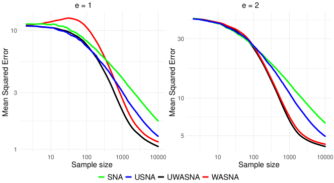
As shown in the figure 1, the weighted averaged estimators converge more rapidly than the other two methods. Both USNA and UWASNA perform comparably to SNA and WASNA in accurately estimating the true coefficients of the logistic regression model. Remarkably, USNA and UWASNA achieve this without using the Riccati formula.

5.2.2 Geometric Median

Next, we conduct simulations in the context of geometric median estimation for a multivariate distribution. We focus on the model introduced by Godichon-Baggioni and Lu, (2023). We generate $n=10\,000$ copies of the random vector $X$ of $\mathbb{R}^{p}$ with $p=10$, where $X\sim\mathcal{N}\left(0,\bf{\Sigma}\right)$ with $\bf{\Sigma}_{i,j}=|i-j|^{0.5}$. Recall that the geometric median is defined by:

$$m=\operatorname*{arg\,min}_{h\in\mathbb{R}^{p}}\mathbb{E}\left[\left\|X-h\right\|-\left\|X\right\|\right].$$

In this model, the result leads to $m=(0,\ldots,0)^{T}$ in this model. In addition, the Hessian matrix $H$ is defined by:

$$H=\mathbb{E}\left[\frac{1}{\left\|X-m\right\|}\left(I_{p}-\frac{(X-m)(X-m)^{T}}{\left\|X-m\right\|^{2}}\right)\right].$$

In this context, algorithm (11)-(13) can be used to estimate $m$ taking $\nabla_{h}g(X_{n},m_{n-1}^{SN})=-\frac{X_{n}-m_{n-1}}{\left\|X_{n}-m_{n-1}\right\|}$ and $\varphi_{n}=\nabla_{h}g(X_{n},m_{n-1}^{SN}+\alpha_{n}Z_{n})-\nabla_{h}(X_{n},m_{n-1}^{SN})$, where $\alpha_{n}=\frac{1}{n\ln{(n+1)}}$ and $(Z_{n})_{n\geq 1}$ is a sequence of independent standard Gaussian vectors.

For a comprehensive evaluation of our methods’ effectiveness in geometric median estimation, we also compare them against two baselines : SNA and WASNA. For all four algorithms, we initialize the estimate of the geometric median with $m_{init}=e\epsilon,$ where $\epsilon\sim\mathcal{N}\left(0,I_{p+1}\right)$ and $e=1$ or $2$. Throughout the simulations, we recorded the MSE of the estimated medians for the four algorithms. The simulation results were averaged over multiple iterations ($N=100$).

Refer to caption
Figure 2: Evolution of the mean squared error with respect to the sample size for geometric median estimation.

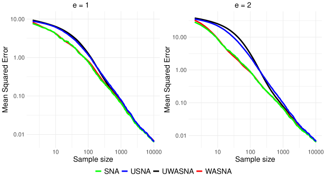
In Figure 2, the results consistently indicate that when the sample size is relatively small (around 100), USNA and UWASNA converge slightly slower. However, beyond that point, they achieve performance on par with both WASNA and SNA in estimating the geometric median.

5.3 Cases where the Riccati formula cannot be used

In this section, we focus on the scenarios where using the Riccati formula in SNA or WASNA is not feasible. We explore the performance of USNA and UWASNA in contrast to an alternative averaged stochastic gradient-based method (”ASGD”) proposed by Polyak and Juditsky, (1992), which is defined as:

$\displaystyle\theta_{n}^{SGD}$ $\displaystyle=\theta_{n-1}^{SGD}-\eta_{n}\nabla_{h}g(X_{n},\theta_{n-1}^{SGD})$ (14)
$\displaystyle\theta_{n}^{ASGD}$ $\displaystyle=\theta_{n-1}^{ASGD}+1/n(\theta_{n}^{SGD}-\theta_{n-1}^{ASGD})$ (15)

where $(\eta_{n})_{n\geq 1}$ is a sequence of learning rates and $\theta_{0}^{ASGD}=\theta_{0}^{SGD}$.

5.3.1 Spherical Distribution

In this paragraph, we focus on the estimation of the parameters of a spherical distribution (Godichon-Baggioni and Portier,, 2017). The aim of the task is to fit a sphere onto a 3D point cloud with noise. In this context, we assume that the observations represent independent realizations of a random vector $X$, which is defined as

$$X=\mu+rWU,$$

where $U$ is uniformly distributed on the unit sphere of $\mathbb{R}^{3}$, $W\sim\mathcal{U}\left([1-\delta,1+\delta]\right)$ with $\delta>0$, $W$ and $U$ are independent. The radius $r>0$ and the center $\mu\in\mathbb{R}^{3}$ are parameters to be estimated. The unknown parameter $\theta=(\mu,r)^{T}$ is a local minimizer of the function $G:\mathbb{R}^{3}\times\mathbb{R}_{+}^{*}\longrightarrow\mathbb{R}$ defined for all $h=(a,b)\in\mathbb{R}^{3}\times\mathbb{R}_{+}^{*}$ by:

$$G(h):=\mathbb{E}\left[g(X,h)\right]=\frac{1}{2}\mathbb{E}\left[\left(\left\|X-a\right\|-b\right)^{2}\right].$$

In this scenario, one can use algorithm (14)-(15) to estimate $\theta$ with

$$\nabla_{h}g(X,h)=\begin{pmatrix}a-X+\frac{b(X-a)}{\left\|X-a\right\|}\\ b-\left\|X-a\right\|\end{pmatrix}.$$

Second-order methods USNA and UWASNA can also be used with

$$\nabla^{2}_{h}g(X,h)=\begin{pmatrix}\left(1-\frac{b}{\left\|X-a\right\|}\right)I_{3}+\frac{b(X-a)(X-a)^{T}}{\left\|X-a\right\|^{3}}&\frac{X-a}{\left\|X-a\right\|}\\ \frac{(X-a)^{T}}{\left\|X-a\right\|}&1\end{pmatrix}.$$

We emphasize that in this specific case, neither the conventional Stochastic Newton Algorithms (SNA) nor the Weighted Averaged version (WASNA) using the Riccati formula are applicable due to the nature of the problem. Thus, we conduct simulations to compare the performance of the USNA, UWASNA, and ASGD. The synthetic datasets were generated with a sample size of $10\,000$ and the true parameters of the spherical distribution were set as follows: $\mu=(0,0,0)$ and $r=2$. In addition, we set $\delta=0.2$, which results in a Hessian matrix with eigenvalues of different order sizes. For all three algorithms, we initialize the estimate of the parameter by

$$\theta_{init}=(\mu_{init},r_{init})^{T}=(0,0,0,2)^{T}+e\epsilon$$

where $\epsilon\sim\mathcal{N}\left(0,I_{4}\right)$ and $e=0.5$ or $1$. Multiple iterations ($N=100$) were performed to reduce the impact of sampling variations.

Refer to caption
Figure 3: Evolution of the mean squared error with respect to the sample size for parameters estimation in a spherical Gaussian distribution.

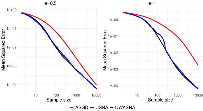
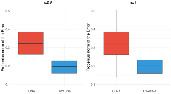
Figure 3 illustrates the comparison between the performances of USNA, UWASNA and ASGD in terms of the mean squared error (MSE) of the estimated parameters. Throughout the simulations, UWASNA amd USNA demonstrate superior performance in accurately estimating the parameters of the spherical distribution when compared to the gradient-based method. Additionally, the Hessian matrix $H$ of the model can be explicitly calculated (Godichon-Baggioni and Portier,, 2017), one has

$$H=\begin{pmatrix}I_{3}-\frac{2}{3}I_{3}\mathbb{E}\left[W\right]\left[W^{-1}\right]&0\\ 0&1\end{pmatrix}.$$

Note that this matrix is diagonal, making its inverse computation straightforward. Therefore, we investigate the Frobenius norm of the difference between the estimated matrix $A_{n}$ and the true matrix $H^{-1}$. From Figure 4, it’s evident that our methods provide a good estimation of the inverse of the Hessian matrix. Moreover, UWASNA offers a better estimation compared to USNA.

Refer to caption
Figure 4: Frobenius norm of the difference between the estimated matrix $A_{n}$ and the true matrix $H^{-1}$.

5.3.2 p-means

Now we focus on the estimation of p-means of a multivariate distribution (Fréchet,, 1948). We consider a random vector $X$ of $\mathbb{R}^{d}$ with $d=40$, where $X\sim\mathcal{N}\left(0,\bf{\Sigma}\right)$ with $\bf{\Sigma}_{i,j}=|i-j|^{0.5}$. The p-mean $m$ of $X$ is defined as the minimizer of the functional $G_{p}:\mathbb{R}^{d}\rightarrow\mathbb{R}$ given for all $h\in\mathbb{R}^{d}$ by:

$$G_{p}(h)=\dfrac{1}{p}\,\mathbb{E}\left[\left\|X-h\right\|^{p}\right],$$

where $1\leq p<+\infty$. Note that in our model $m=(0,\ldots,0)^{T}$. We can easily verify that the gradient and the Hessian of $G_{p}$ are given by:

$\displaystyle\nabla G_{p}(h)$ $\displaystyle=-\mathbb{E}\left[(X-h)\left\|X-h\right\|^{p-2}\right],$
$\displaystyle\nabla^{2}G_{p}(h)$ $\displaystyle=\mathbb{E}\left[\left\|X-h\right\|^{p-2}\left(I_{d}-(2-p)\frac{(X-h)(X-h)^{T}}{\left\|X-h\right\|^{2}}\right)\right].$

We aim to compare the performance of USNA, UWASNA, and ASGD for estimating the p-mean of $X$ through simulations. We consider the case $p=1.5$ and we simulate $N=100$ independent samples of size $n=10\,000$. For all three algorithms, we initialize the estimate with $m_{init}=e\epsilon$ where $\epsilon\sim\mathcal{N}(0,I_{d})$ and $e=1$ or $2$.

Refer to caption
Figure 5: Evolution of the mean squared error with respect to the sample size for p-means estimation.

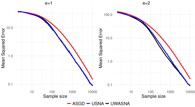
As depicted in the Figure 5, we plotted the MSE versus sample size. It is evident that USNA and UWASNA consistently outperforms ASGD in estimating the p-means. Their superior performance can be attributed to the incorporation of information from the Hessian matrix. These results further emphasize the advantage of using USNA and UWASNA as alternative methods when it is impossible to use the Riccati formula.

5.4 Application to real data

We apply the algorithms to ”COVTYPE” dataset, a well-known dataset used for classification tasks (Blackard and Dean,, 1999; Schmidt et al.,, 2017; Toulis et al.,, 2016). The original study was based on a dataset comprising 581,011 observations and 54 predictors. The primary objective was to predict the cover type of forests within Roosevelt National Park. In our current investigation, we will narrow our focus to the most prevalent category of the target variable, which is ”Spruce/Fir,” accounting for 49% of the observations. As a result, we convert the ”covertype” variable into a binary form, with the ”fir” category assigned a value of 1, while all other categories are assigned a value of 0. The objective is to use logistic regression to predict the variable ”covertype”. We split the dataset into training (80%) and test (20%) sets.

We implement the UWASNA, USNA, WASNA and SNA on the training set. As a baseline, we also apply a first-order algorithm ASGD on it. We evaluate the performance of each algorithm by calculating the accuracy of each one on both training set and test set. The results are summarized in Table 1.

UWASNA USNA WASNA SNA ASGD
Training Accuracy(%) 75.63 75.31 75.52 75.38 74.54
Test Accuracy(%) 75.61 75.34 75.50 75.33 74.64
Table 1: Accuracy of UWASNA, USNA, WASNA, SNA and ASGD algorithms on ”COVTYPE” dataset.

We observe that UWASNA, USNA, WASNA and SNA demonstrate similar performances, and they achieve higher accuracies on both training set and test set compared to ASGD. By successfully applying USNA and UWASNA on this dataset, we illustrate their practicality in real-world applications.

Conclusion

In this study, we thoroughly examined the stochastic optimization problem, primarily focusing on accurately estimating the unknown parameter. Our significant contribution is the introduction of a direct method to estimate the inverse of the Hessian matrix. Instead of the traditional approach, which estimates the Hessian matrix first, we directly addressed its inverse, using the Robbins-Monro procedure.

This approach led us to develop the Universal Weighted Averaged Stochastic Newton Algorithm. Through our extensive testing, we found that our newly proposed methods are both efficient and robust. When compared with standard first and second-order algorithms, our method consistently performed well. In certain scenarios, it even outperformed these conventional algorithms.

In summary, our findings emphasize the potential of second-order methods in optimization. Our approach to directly estimating the Hessian matrix’s inverse represents a significant advancement, combining simplicity with efficiency.

6 Proofs

For the sake of simplicity, in the following we denote $T_{n}:=\nabla^{2}_{h}g(X_{n},\hat{\theta}_{n-1})Z_{n}Z_{n}^{T}$. Recall that $\left\|Z_{n}\right\|$ is bounded, i.e there is $M$ such that $\left\|Z\right\|\leq M$. In addition, let us recall that if $\left\|Q_{n+1}\right\|\left\|Z_{n+1}\right\|\leq\beta_{n+1}$, it then follows that $\left\|T_{n+1}\right\|_{op}\leq\beta_{n+1}$.

6.1 Study on the largest eigenvalue of $A_{n}$

The following proposition provides an initial asymptotic bound of the largest eigenvalue of $A_{n}$ without requiring knowledge on the behavior of the estimate $\hat{\theta}_{n}$. This result is crucial to prove Theorems 3.1 and 4.1.

Proposition 6.1.

Under Assumptions (A3) and (A5), the largest eigenvalue of $A_{n}$ denoted by $\lambda_{\max}(A_{n})$ satisfies for all $\delta>0$

$$\lambda_{\max}(A_{n})=o\left(n^{1-\gamma}\ln n^{1+\delta}\right)a.s.\quad\text{and}\quad\lambda_{\max}(A_{n},\tau)=o\left(n^{1-\gamma}\ln n^{1+\delta}\right)a.s.$$
Proof of Proposition 6.1.

Define $W_{n}:=A_{n-1}T_{n}^{T}+T_{n}A_{n-1}$. By definition of $A_{n}$,

$\displaystyle\left\|A_{n+1}\right\|_{F}^{2}$ $\displaystyle=\left\|A_{n}\right\|_{F}^{2}-2\gamma_{n+1}\braket{A_{n},W_{n+1}-2I_{d}}_{F}\mathbf{1}_{\left\|Q_{n+1}\right\|\left\|Z_{n+1}\right\|\leq\beta_{n+1}}$
$\displaystyle+\gamma_{n+1}^{2}\left\|W_{n+1}-2I_{d}\right\|^{2}_{F}\mathbf{1}_{\left\|Q_{n+1}\right\|\left\|Z_{n+1}\right\|\leq\beta_{n+1}}.$

Therefore,

$\displaystyle\mathbb{E}\left[\left\|A_{n+1}\right\|_{F}^{2}|\mathcal{F}_{n}\right]$ $\displaystyle=\left\|A_{n}\right\|_{F}^{2}-2\gamma_{n+1}\braket{A_{n},\nabla^{2}G(\hat{\theta}_{n})A_{n}+A_{n}\nabla^{2}G(\hat{\theta}_{n})-2I_{d}}_{F}$
$\displaystyle+\gamma_{n+1}^{2}\mathbb{E}\left[\left\|W_{n+1}-2I_{d}\right\|^{2}\mathbf{1}_{\left\|Q_{n+1}\right\|\left\|Z_{n+1}\right\|\leq\beta_{n+1}}|\mathcal{F}_{n}\right]$
$\displaystyle+2\gamma_{n+1}\mathbb{E}\left[\braket{A_{n},W_{n+1}-2I_{d}}_{F}\mathbf{1}_{\left\|Q_{n+1}\right\|\left\|Z_{n+1}\right\|>\beta_{n+1}}|\mathcal{F}_{n}\right].$

Assumption (A5) ensures that

$\displaystyle\mathbb{E}$ $\displaystyle\left[\left\|W_{n+1}-2I_{d}\right\|^{2}_{F}\mathbf{1}_{\left\|Q_{n+1}\right\|\left\|Z_{n+1}\right\|\leq\beta_{n+1}}|\mathcal{F}_{n}\right]$
$\displaystyle\leq 8\left(\mathbb{E}\left[\left\|\nabla^{2}_{h}g(X_{n+1},\hat{\theta}_{n})\right\|_{F}^{2}\right]\mathbb{E}\left[\left\|Z_{n+1}\right\|^{4}\right]\left\|A_{n}\right\|^{2}_{F}+d\right)$
$\displaystyle\leq 8\left(C_{q}^{2/q}\left\|A_{n}\right\|^{2}_{F}+d\right).$

Since $\left\|Q_{n+1}\right\|$ = $\left\|Q_{n+1}\right\|^{q}\left\|Q_{n+1}\right\|^{1-q}$ with $q>1$, for any $\zeta_{n}>0$,

$\displaystyle\gamma_{n+1}$ $\displaystyle\mathbb{E}\left[\braket{A_{n},W_{n+1}-2I_{d}}_{F}\mathbf{1}_{\left\|Q_{n+1}\right\|\left\|Z_{n+1}\right\|>\beta_{n+1}}|\mathcal{F}_{n}\right]$
$\displaystyle\leq 2\gamma_{n+1}\left\|A_{n}\right\|^{2}_{F}\mathbb{E}\left[\left\|Q_{n+1}\right\|\left\|Z_{n+1}\right\|\mathbf{1}_{\left\|Q_{n+1}\right\|\left\|Z_{n+1}\right\|\geq\beta_{n+1}}|\mathcal{F}_{n}\right]$
$\displaystyle+\frac{\gamma_{n+1}}{\zeta_{n+1}}\left\|A_{n}\right\|^{2}_{F}+\zeta_{n+1}d$
$\displaystyle\leq\left(2C_{q}M^{2q}\gamma_{n+1}\beta_{n+1}^{1-q}+\frac{\gamma_{n+1}}{\zeta_{n+1}}\right)\left\|A_{n}\right\|^{2}_{F}+\gamma_{n+1}\zeta_{n+1}d.$

Since $\nabla^{2}G(\hat{\theta}_{n})$ and $A_{n}$ are positive, one has for any $\zeta_{n}>0$,

$\displaystyle-\gamma_{n+1}\braket{A_{n},\nabla^{2}G(\hat{\theta}_{n})A_{n}+A_{n}\nabla^{2}G(\hat{\theta}_{n})-2I_{d}}_{F}$ $\displaystyle\leq\gamma_{n+1}\braket{A_{n},2I_{d}}$
$\displaystyle\leq\frac{\gamma_{n+1}}{\zeta_{n+1}}\left\|A_{n}\right\|^{2}_{F}+\gamma_{n+1}\zeta_{n+1}d.$

Finally,

$\displaystyle\mathbb{E}\left[\left\|A_{n+1}\right\|_{F}^{2}|\mathcal{F}_{n}\right]$ $\displaystyle\leq\left(1+\frac{4\gamma_{n+1}}{\zeta_{n+1}}+4C_{q}\gamma_{n+1}\beta_{n+1}^{1-q}+8\gamma_{n+1}^{2}C_{q}^{2/q}\right)\left\|A_{n}\right\|_{F}^{2}$
$\displaystyle+4\gamma_{n+1}\zeta_{n+1}d+8\gamma_{n+1}^{2}d.$

Setting $\zeta_{n}=n^{1-\gamma}\ln n^{1+\delta}$ with $\delta>0$, we can apply Lemma 6.2 with $V_{n}=\left\|A_{n}\right\|_{F}^{2}$, and $a_{n}=\zeta_{n}^{2}$. One then obtains $\left\|A_{n}\right\|_{F}^{2}=o\left(\zeta_{n}^{2}\right)=o\left(n^{2-2\gamma}\ln n^{2+2\delta}\right)$, so that $\lambda_{\max}(A_{n})=o\left(n^{1-\gamma}\ln n^{1+\delta}\right)a.s.$

6.2 Proof of Theorem 3.1

The aim is to provide an initial rate of convergence for $A_{n}$. A more refined or faster rate will be established later. First, note that

$\displaystyle A_{n+1}-H^{-1}$ $\displaystyle=A_{n}-H^{-1}-\gamma_{n+1}(W_{n+1}-2I_{d})\mathbf{1}_{\left\|Q_{n+1}\right\|\left\|Z_{n+1}\right\|\leq\beta_{n+1}}$
$\displaystyle=A_{n}-H^{-1}-\gamma_{n+1}(W_{n+1}-2I_{d})+\gamma_{n+1}(W_{n+1}-2I_{d})\mathbf{1}_{\left\|Q_{n+1}\right\|\left\|Z_{n+1}\right\|>\beta_{n+1}}$
$\displaystyle=A_{n}-H^{-1}-\gamma_{n+1}\left(\mathbb{E}\left[W_{n+1}|\mathcal{F}_{n}\right]-2I_{d}\right)+\gamma_{n+1}\xi_{n+1}$
$\displaystyle\quad+\gamma_{n+1}(W_{n+1}-2I_{d})\mathbf{1}_{\left\|Q_{n+1}\right\|\left\|Z_{n+1}\right\|>\beta_{n+1}}$
$\displaystyle=A_{n}-H^{-1}-\gamma_{n+1}\left(\nabla^{2}G(\hat{\theta}_{n})A_{n}+A_{n}\nabla^{2}G(\hat{\theta}_{n})-2I_{d}\right)+\gamma_{n+1}\xi_{n+1}+$
$\displaystyle\quad\gamma_{n+1}(W_{n+1}-2I_{d})\mathbf{1}_{\left\|Q_{n+1}\right\|\left\|Z_{n+1}\right\|>\beta_{n+1}}$

where $\xi_{n+1}:=-W_{n+1}+\nabla^{2}G(\hat{\theta}_{n})A_{n}+A_{n}\nabla^{2}G(\hat{\theta}_{n})$. Let $\alpha^{*}_{k}$ be the function defined for all $h\in\mathcal{M}_{p}(\mathbb{R})$ by

$$\alpha^{*}_{k}(h)=\left(I_{d}-\gamma_{k+1}H\right)h\left(I_{d}-\gamma_{k+1}H\right),$$

we then have

$\displaystyle A_{n+1}-A$ $\displaystyle=\alpha_{n}^{*}\left(A_{n}-H^{-1}\right)-\gamma_{n+1}^{2}H(A_{n}-H^{-1})H$
$\displaystyle+\gamma_{n+1}r_{1,n}+\gamma_{n+1}r_{2,n}+\gamma_{n+1}s_{n}+\gamma_{n+1}s^{\prime}_{n}+\gamma_{n+1}\xi_{n+1}$ (16)

where

$\displaystyle r_{1,n}$ $\displaystyle=(\nabla^{2}G(\hat{\theta}_{n})-H)H^{-1}+H^{-1}(\nabla^{2}G(\hat{\theta}_{n})-H),$
$\displaystyle r_{2,n}$ $\displaystyle=(W_{n+1}-2I_{d})\mathbf{1}_{\left\|Q_{n+1}\right\|\left\|Z_{n+1}\right\|>\beta_{n+1}}-\mathbb{E}\left[(W_{n+1}-2I_{d})\mathbf{1}_{\left\|Q_{n+1}\right\|\left\|Z_{n+1}\right\|>\beta_{n+1}}|\mathcal{F}_{n}\right],$
$\displaystyle s_{n}$ $\displaystyle=\mathbb{E}\left[\left(T_{n+1}\left(A_{n}-H^{-1}\right)+\left(A_{n}-H^{-1}\right)T_{n+1}\right)\mathbf{1}_{\left\|Q_{n+1}\right\|\left\|Z_{n+1}\right\|>\beta_{n+1}}|\mathcal{F}_{n}\right]$
$\displaystyle+\left(\nabla^{2}G(\hat{\theta}_{n})-H\right)\left(A_{n}-H^{-1}\right)+\left(A_{n}-H^{-1}\right)\left(\nabla^{2}G(\hat{\theta}_{n})-H\right),$
$\displaystyle s^{\prime}_{n}$ $\displaystyle=\mathbb{E}\left[\left(T_{n+1}H^{-1}+H^{-1}T_{n+1}-2I_{d}\right)\mathbf{1}_{\left\|Q_{n+1}\right\|\left\|Z_{n+1}\right\|>\beta_{n+1}}|\mathcal{F}_{n}\right]$

By induction,

$\displaystyle A_{n}-H^{-1}$ $\displaystyle=\Psi^{*}_{n,0}\left(A_{0}-H^{-1}\right)+\sum_{k=0}^{n-1}\Psi^{*}_{n,k+1}\gamma_{k+1}\xi_{k+1}+\sum_{k=0}^{n-1}\Psi^{*}_{n,k+1}\gamma_{k+1}r_{1,k}$
$\displaystyle\quad+\sum_{k=0}^{n-1}\Psi^{*}_{n,k+1}\gamma_{k+1}r_{2,k}+\sum_{k=0}^{n-1}\Psi^{*}_{n,k+1}\gamma_{k+1}s_{k}+\sum_{k=0}^{n-1}\Psi^{*}_{n,k+1}\gamma_{k+1}s^{\prime}_{k},$ (17)

where $\Psi^{*}_{n,k}$ is the function defined for all $h\in\mathcal{M}_{p}(\mathbb{R})$ by :

$$\Psi^{*}_{n,k}(h)=\left(\prod_{j=k+1}^{n}\alpha^{*}_{j}\right)(h)=\left(\prod_{j=k+1}^{n}\left(I_{d}-\gamma_{j}H\right)\right)h\left(\prod_{j=k+1}^{n}\left(I_{d}-\gamma_{j}H\right)\right).$$

Next, we will determine the rate of convergence for each term on the right-hand side of equation (6.2).

Rate of convergence of $M_{n}:=\sum_{k=0}^{n-1}\Psi^{*}_{n,k+1}\gamma_{k+1}\xi_{k+1}$: Recall that for all $\delta>0$, $\lambda_{\max}(A_{n})=o\left(n^{1-\gamma}\ln n^{1+\delta}\right)a.s.$ Thus, there exists a constant $c^{\prime}>0$ such that $\mathbb{E}\left[\left\|\xi_{n+1}\right\|^{2}_{F}|\mathcal{F}_{n}\right]\leq c^{\prime}\left(1+\left\|A_{n}\right\|_{F}^{2}\right)=o\left(n^{2-2\gamma}\ln n^{2+2\delta}\right)$ a.s., and according to Lemma 6.3, it follows that

$$\left\|\sum_{k=0}^{n-1}\Psi^{*}_{n,k+1}\gamma_{k+1}\xi_{k+1}\right\|^{2}_{F}=\mathcal{O}\left(n^{2-3\gamma}\ln n^{2+2\delta}\right)\quad a.s.$$ (18)

Rate of convergence of $R_{1,n}:=\sum_{k=0}^{n-1}\Psi^{*}_{n,k+1}\gamma_{k+1}r_{1,k}$: we have

$$R_{1,n+1}=\left(I_{d}-\gamma_{n+1}H\right)R_{1,n}\left(I_{d}-\gamma_{n+1}H\right)+\gamma_{n+1}r_{1,n+1}.$$

Therefore, for $n$ large enough

$\displaystyle\left\|R_{1,n+1}\right\|_{op}$ $\displaystyle\leq\left\|I_{d}-\gamma_{n+1}H\right\|^{2}_{op}\left\|R_{1,n}\right\|_{op}+\gamma_{n+1}\left\|r_{1,n+1}\right\|_{op}$
$\displaystyle\leq\left(1-\lambda_{\min}(H)\gamma_{n+1}\right)^{2}\left\|R_{1,n}\right\|_{op}+\gamma_{n+1}\left\|r_{1,n+1}\right\|_{op}a.s.$

By Assumption (A4), $\left\|r_{1,n+1}\right\|_{op}=o\left(n^{-a/2}\ln n^{(1+\delta)/2}\right)a.s.$ According to Lemma 6.4,

$$\left\|R_{1,n+1}\right\|_{op}=o\left(n^{-a/2}\ln n^{(1+\delta)/2}\right)\quad a.s.$$ (19)

Rate of convergence of $R_{2,n}:=\sum_{k=0}^{n-1}\Psi^{*}_{n,k+1}\gamma_{k+1}r_{2,k}$:

$\displaystyle\mathbb{E}$ $\displaystyle\left[\left\|(W_{n+1}-2I_{d})\mathbf{1}_{\left\|Q_{n+1}\right\|\left\|Z_{n+1}\right\|\geq\beta_{n+1}}\right\|_{op}^{2}|\mathcal{F}_{n}\right]$
$\displaystyle\leq$ $\displaystyle 12\mathbb{E}\left[\left(\left\|Q_{n+1}\right\|^{2}\left\|Z_{n+1}\right\|^{2}\left\|A_{n}\right\|^{2}+d\right)\mathbf{1}_{\left\|Q_{n+1}\right\|\left\|Z_{n+1}\right\|\geq\beta_{n+1}}|\mathcal{F}_{n}\right].$

Applying Markov’s inequality, and since $\left\|Z_{n}\right\|$ is supposed to be bounded by $M$,

$\displaystyle\mathbb{E}\left[\left\|(W_{n+1}-2I_{d})\mathbf{1}_{\left\|Q_{n+1}\right\|\left\|Z_{n+1}\right\|\geq\beta_{n+1}}\right\|^{2}|\mathcal{F}_{n}\right]$ $\displaystyle\leq 12d\mathbb{E}\left[\left\|\nabla^{2}g(X_{n+1},\hat{\theta}_{n})\right\|_{op}^{q}\left\|Z_{n}Z_{n}^{T}\right\|^{q}|\mathcal{F}_{n}\right]\beta_{n}^{-q}$
$\displaystyle+12\left\|A_{n}\right\|^{2}\mathbb{E}\left[\left\|Q_{n}\right\|^{2}M^{2}\mathbf{1}_{\left\|Q_{n+1}\right\|\left\|Z_{n+1}\right\|\geq\beta_{n+1}}\right]$
$\displaystyle\leq 12dM^{2q}\mathbb{E}\left[\left\|\nabla^{2}g(X_{n+1},\hat{\theta}_{n})\right\|_{op}^{q}|\mathcal{F}_{n}\right]\beta_{n}^{-q}$
$\displaystyle+12C_{q}\left\|A_{n}\right\|^{2}\beta_{n+1}^{2-q}$

Thus, by Lemma 6.4,

$$\left\|R_{2,n}\right\|^{2}_{op}=\mathcal{O}\left(n^{2-3\gamma}\ln n^{2+2\delta}n^{2\beta-q\beta}\right)\quad a.s.$$ (20)

Note that the rate of convergence for $R_{2,n}$ is faster than that of $M_{n}$.

Rate of convergence of $S_{n}^{\prime}:=\sum_{k=0}^{n-1}\Psi^{*}_{n,k+1}\gamma_{k+1}s^{\prime}_{k}$: We have similarly

$\displaystyle\left\|s^{\prime}_{n}\right\|$ $\displaystyle\leq\mathbb{E}\left[\left\|\left(T_{n+1}H^{-1}+H^{-1}T_{n+1}-2I_{d}\right)\right\|_{F}\mathbf{1}_{\left\|Q_{n+1}\right\|\left\|Z_{n+1}\right\|\geq\beta_{n+1}}|\mathcal{F}_{n}\right]$
$\displaystyle\leq 2\left\|H^{-1}\right\|_{F}\mathbb{E}\left[\left\|Z_{n+1}\right\|^{2}\left\|\nabla_{h}^{2}g\left(X_{n+1},\hat{\theta}_{n}\right)\right\|_{F}\mathbf{1}_{\left\|Q_{n+1}\right\|\left\|Z_{n+1}\right\|\geq\beta_{n+1}}|\mathcal{F}_{n}\right]$
$\displaystyle+2q\mathbb{E}\left[\mathbf{1}_{\left\|Q_{n+1}\right\|\left\|Z_{n+1}\right\|\geq\beta_{n+1}}|\mathcal{F}_{n}\right]=\mathcal{O}\left(\beta_{n}^{1-q}\right).$

Therefore, thanks to Lemma 6.4,

$$S^{\prime}_{n}=\mathcal{O}\left(\beta_{n}^{1-q}\right).$$ (21)

A first result for $A_{n}$: Thanks to equalities (18) to (21), one can rewrite $A_{n}-H^{-1}$ as

$$A_{n}-H^{-1}=\sum_{k=0}^{n-1}\Psi^{*}_{n,k+1}\gamma_{k+1}s_{k}+\widetilde{S}_{n}$$

with $\left\|\widetilde{S}_{n}\right\|_{F}=o\left(n^{\max\left(1-\frac{3}{2}\gamma,-a/2,\beta(1-q)\right)}\ln n^{1+\delta}\right).$ In addition, we have

$\displaystyle\left\|s_{n}\right\|_{op}$ $\displaystyle\leq\left\|A_{n}-H^{-1}\right\|_{op}\mathbb{E}\left[\left\|Q_{n+1}\right\|\left\|Z_{n+1}\right\|\mathbf{1}_{\left\|Q_{n+1}\right\|\left\|Z_{n+1}\right\|\geq\beta_{n}}\|\mathcal{F}_{n}\right]$
$\displaystyle\quad+\left\|\nabla^{2}G(\hat{\theta}_{n})-H\right\|\left\|A_{n}-H^{-1}\right\|_{op}$
$\displaystyle=o\left(\left\|A_{n}-H^{-1}\right\|_{op}\right)\quad a.s.$

Define $S_{n}:=\sum_{k=0}^{n-1}\Psi^{*}_{n,k+1}\gamma_{k+1}s_{k}$. There exists a positive sequence $(\widetilde{r}_{n})_{n\geq 0}$ with $\widetilde{r}_{n}\xrightarrow[n\rightarrow\infty]{a.s.}0$ such that

$\displaystyle\left\|S_{n+1}\right\|_{op}$ $\displaystyle\leq(1-\lambda_{\min}(H)\gamma_{n+1})^{2}\left\|S_{n}\right\|_{op}+\gamma_{n+1}\widetilde{r}_{n}\left\|A_{n}-H^{-1}\right\|_{op}$
$\displaystyle\leq(1-\lambda_{\min}(H)\gamma_{n+1})^{2}\left\|S_{n}\right\|_{op}+\gamma_{n+1}\widetilde{r}_{n}\left(\left\|S_{n}\right\|_{op}+\left\|\widetilde{S}_{n}\right\|_{op}\right).$

Applying Lemma 6.4,

$$\left\|S_{n}\right\|_{op}=o\left(n^{\max\left(1-\frac{3}{2}\gamma,-a/2,\beta(1-q)\right)}\ln n^{1+\delta}\right),$$

which implies that

$$\left\|A_{n}-H^{-1}\right\|_{F}=o\left(n^{\max\left(1-\frac{3}{2}\gamma,-a/2,\beta(1-q)\right)}\ln n^{1+\delta}\right)a.s.$$

Final rate of convergence of $A_{n}$: The aim here is, with the help of this first result on $A_{n}$, to give better rates of convergence for $M_{n}$ and $R_{2,n}$. First, note that if $\gamma>2/3$, then $1-\frac{3}{2}\gamma<0$ and we have directly $A_{n}\xrightarrow[n\rightarrow\infty]{a.s.}H^{-1}$. If $\gamma\leq 2/3$, we have $1-\frac{3}{2}\gamma>0$ , so that $\max\{1-\frac{3}{2}\gamma,-a/2,\beta(1-q)\}=\max\{1-\frac{3}{2}\gamma,\beta(1-q)\}$ and $\left\|A_{n}\right\|=o\left(n^{\max\{1-\frac{3}{2}\gamma,\beta(1-q)\}}\ln n^{1+\delta}\right)a.s.$. Thus, applying Lemma 6.3 in the worse case (i.e when $\gamma>2/3$), one now has

$$\left\|M_{n}\right\|_{F}^{2}=o\left(n^{\max\{2-4\gamma,\beta(2-2q)-\gamma\}}\ln n^{2+2\delta}\right)\quad a.s.$$

and

$$\left\|R_{2,n}\right\|^{2}_{op}=\mathcal{O}\left(n^{2-4\gamma}\ln n^{2+2\delta}n^{2\beta-q\beta}\right)\quad a.s.$$

Following the same process as before, we now have that for any $\gamma\in(1/2,1)$, $A_{n}$ converges almost surely to $H^{-1}$, and in particular, one has $\left\|A_{n}\right\|$ = $\mathcal{O}\left(1\right)$. Applying another time Lemma 6.3, we have

$$\left\|M_{n}\right\|_{F}^{2}=\mathcal{O}\left(n^{-\gamma}\ln n^{1+\delta}\right)\quad a.s.$$

and

$$\left\|R_{2,n}\right\|^{2}_{op}=\mathcal{O}\left(n^{-\gamma}\ln n^{2+2\delta}n^{2\beta-q\beta}\right)\quad a.s.$$

Finally, we have

$$\left\|A_{n}-H^{-1}\right\|_{F}^{2}=o\left(\frac{\ln n^{1+\delta}}{n^{\min\{\gamma,a,2\beta(q-1)\}}}\right)a.s.$$ (22)

Rate of convergence of $A_{n,\tau}$. Decomposition (16) can be written as

$\displaystyle H(A_{n}-H^{-1})+(A_{n}-H^{-1})H=\frac{A_{n}-H^{-1}-(A_{n+1}-H^{-1})}{\gamma_{n+1}}+r_{1,n}+r_{2,n}+s_{n}+s^{\prime}_{n}+\xi_{n+1},$

so that

$\displaystyle H(A_{n,\tau}-H^{-1})+(A_{n,\tau}-H^{-1})H=$ $\displaystyle t_{n}\sum_{k=0}^{n}u_{k}\left((A_{k}-H^{-1})-(A_{k+1}-H^{-1})\right)$
$\displaystyle+t_{n}\sum_{k=0}^{n}u_{k}\gamma_{k+1}(r_{1,n}+r_{2,n}+s_{n}+s^{\prime}_{n}+\xi_{n+1})$ (23)

where $t_{n}=\frac{1}{\sum^{n}_{k=0}\log(k+1)^{\tau}}$ and $u_{k+1}=\frac{\ln(k+1)^{\tau}}{\gamma_{k+1}}$. Our objective is to determine the rate of convergence for each term on the right-hand side of the decomposition given in (6.2).

Rate of convergence of $t_{n}\sum_{k=0}^{n}u_{k+1}\left((A_{k}-H^{-1})-(A_{k+1}-H^{-1})\right)$: with the help of an Abel’s transform,

$\displaystyle t_{n}\sum_{k=0}^{n}u_{k+1}\left((A_{k}-H^{-1})-(A_{k+1}-H^{-1})\right)$ $\displaystyle=-t_{n}\left(A_{n+1}-H^{-1}\right)u_{n+1}+t_{n}\left(A_{0}-H^{-1}\right)u_{1}$
$\displaystyle+t_{n}\sum_{k=1}^{n}(A_{k}-H^{-1})(u_{k+1}-u_{k}).$

It is obvious that $t_{n}\left(A_{0}-H^{-1}\right)u_{1}$ is negligible while thanks to equality (22),

$$t_{n}\left\|A_{n+1}-H^{-1}\right\|u_{n+1}=o\left(\frac{\ln n^{1+\delta}}{n^{1-\gamma+\frac{1}{2}\min\left\{\gamma,a,2\beta(q-1)\right\}}}\right)\quad a.s$$

In addition, by the mean value theorem, $|u_{k+1}-u_{k}|\leq 2k^{\gamma-1}\max\{1,\tau\}\ln(k+1)^{\tau}$, which implies that

$$\left\|\sum_{k=1}^{n}(A_{k}-H^{-1})(u_{k+1}-u_{k})\right\|_{F}\leq\sum_{k=1}^{n}\left\|A_{k}-H^{-1}\right\|_{F}2k^{\gamma-1}\max\{1,\tau\}\ln(k+1)^{\tau}$$

and with the help of equation (22)

$$\left\|t_{n}\sum_{k=0}^{n}u_{k}\left((A_{k}-H^{-1})-(A_{k+1}-H^{-1})\right)\right\|_{F}=o\left(\frac{\ln n^{1+\delta}}{n^{1-\gamma+\frac{1}{2}\min\left\{\gamma,a,2\beta(q-1)\right\}}}\right)\quad a.s$$

Rate of convergence of $t_{n}\sum_{k=0}^{n}u_{k+1}\gamma_{k+1}\xi_{k+1}$. Remark that there exists $c^{\prime}>0$ such that for all $\delta>0$

$$\mathbb{E}\left[\left\|\xi_{n+1}\right\|^{2}_{F}\|\mathcal{F}_{n}\right]\leq c^{\prime}\left(1+\left\|A_{n}\right\|_{F}^{2}\right)\leq c^{\prime}\left(1+2\left\|A_{n}-H^{-1}\right\|_{F}^{2}+2\left\|H^{-1}\right\|_{F}^{2}\right).$$

By applying a law of large numbers for martingales, one obtains for all $\delta>0$

$$\left\|t_{n}\sum_{k=0}^{n}u_{k+1}\gamma_{k+1}\xi_{k+1}\right\|_{F}^{2}=o\left(\frac{\ln n^{1+\delta}}{n}\right)a.s.$$

Rate of convergence of $t_{n}\sum_{k=0}^{n}u_{k+1}\gamma_{k+1}r_{1,k}$. First, let us give a useful equality: consider $\sum_{k=0}^{n}k^{-\tilde{a}/2}\ln k^{(1+\delta)/2}$ with $\tilde{a}>0$, since $\int_{1}^{n}x^{-\tilde{a}/2}\ln x^{(1+\delta)/2}dx\leq c(\ln n)^{(1+\delta)/2}x^{1-\tilde{a}}$ if $\tilde{a}\neq 2$ and $\int_{1}^{n}x^{-\tilde{a}/2}\ln x^{(1+\delta)/2}dx\leq c^{\prime}(\ln n)^{(3+\delta)/2}$ if $\tilde{a}=2$ then one can verify that

$$\left\|t_{n}\sum_{k=0}^{n}u_{k}\gamma_{k+1}k^{-\tilde{a}/2}\ln k^{(1+\delta)/2}\right\|^{2}_{F}=o\left(\frac{\ln n^{1+\delta+2\mathbf{1}_{\tilde{a}=2}}}{n^{\min\{2,\tilde{a}\}}}\right)a.s.$$ (24)

Then, recalling that $\left\|r_{1,k+1}\right\|_{op}=o\left(n^{-a/2}\ln k^{(1+\delta)/2}\right)$

$$\left\|t_{n}\sum_{k=0}^{n}u_{k}\gamma_{k+1}r_{1,k}\right\|_{F}^{2}=o\left(\frac{\ln n^{1+\delta+2\mathbf{1}_{{a}=2}}}{n^{\min\{2,{a}\}}}\right)a.s.$$

Rate of convergence of $t_{n}\sum_{k=0}^{n}u_{k+1}\gamma_{k+1}s_{k}^{\prime}$. Recalling that $s_{k}^{\prime}=O\left(\beta_{k}^{1-q}\right)$, it comes

$$\left\|t_{n}\sum_{k=0}^{n}u_{k}\gamma_{k+1}s_{k}^{\prime}\right\|_{F}^{2}=o\left(\frac{\ln n^{2\mathbf{1}_{2\beta(q-1)=2}}}{n^{\min\{2,2\beta(q-1)\}}}\right)\quad a.s.$$

Rate of convergence of $t_{n}\sum_{k=0}^{n}u_{k+1}\gamma_{k+1}s_{k}$. Recall that

$\displaystyle\left\|s_{n}\right\|_{op}$ $\displaystyle\leq\left\|A_{n}-H^{-1}\right\|_{op}\mathbb{E}\left[\left\|Q_{n+1}\right\|\left\|Z_{n+1}\right\|\mathbf{1}_{\left\|Q_{n+1}\right\|\left\|Z_{n+1}\right\|\geq\beta_{n}}\|\mathcal{F}_{n}\right]$
$\displaystyle\quad+\left\|\nabla^{2}G(\hat{\theta}_{n})-H\right\|\left\|A_{n}-H^{-1}\right\|_{op},$

Recalling that $\mathbb{E}\left[\left\|T_{n+1}\right\|_{op}\mathbf{1}_{\left\|T_{n+1}\right\|\geq\beta_{n}}|\mathcal{F}_{n}\right]=O\left(\beta_{n}^{1-q}\right)$, and with the help of equality (22)

$\displaystyle\left\|A_{n}-H^{-1}\right\|_{op}\mathbb{E}\left[\left\|Q_{n+1}\right\|\left\|Z_{n+1}\right\|\mathbf{1}_{\left\|Q_{n+1}\right\|\left\|Z_{n+1}\right\|\geq\beta_{n}}\|\mathcal{F}_{n}\right]$
$\displaystyle\quad=o\left(\frac{\ln n^{(1+\delta)/2}}{n^{\beta(q-1)+\frac{1}{2}\min\left\{a,\gamma,2\beta(q-1)\right\}}}\right)\quad a.s$

In addition, one has

$$\left\|\nabla^{2}G(\hat{\theta}_{n})-H\right\|\left\|A_{n}-H^{-1}\right\|_{op}=o\left(\frac{\ln n^{1+\delta}}{n^{a/2+\frac{1}{2}\min\left\{a,\gamma,2\beta(q-1)\right\}}}\right)\quad a.s.$$

leading to

$$\left\|s_{n}\right\|=o\left(\frac{\ln n^{1+\delta}}{n^{\min\left\{a/2,\beta(q-1)\right\}+\frac{1}{2}\min\left\{a,\gamma,2\beta(q-1)\right\}}}\right)\quad a.s.$$

Then, since $\min\left\{a/2,\beta(q-1)\right\}+\frac{1}{2}\min\left\{a,\gamma,2\beta(q-1)\right\}\geq\min\left\{a,\gamma,2\beta(q-1)\right\}$,

$$\left\|t_{n}\sum_{k=0}^{n}u_{k}\gamma_{k+1}s_{k}\right\|_{F}^{2}=o\left(\frac{\ln n^{1+\delta}}{n^{\min\{2,2\min\left\{a,\gamma,2\beta(q-1)\right\}\}}}\right)a.s.$$

Rate of convergence of $t_{n}\sum_{k=0}^{n}u_{k+1}\gamma_{k+1}r_{2,k}$. Let us recall that $r_{2,n}$ is a martingale difference, and with the help of a law of large numbers for martingales it comes that

$$\left\|t_{n}\sum_{k=0}^{n}u_{k+1}\gamma_{k+1}r_{2,k}\right\|_{F}^{2}=o\left(\frac{\ln n^{1+\delta}}{n}\right)\quad a.s.$$

Rate of convergence of $A_{n,\tau}$. We so have

$$\left\|H(A_{n,\tau}-H^{-1})+(A_{n,\tau}-H^{-1})H\right\|^{2}=o\left(\frac{\ln n^{1+\delta}}{n^{\min\{1,a,2\beta(q-1)\}}}\right)a.s.$$

Note that $H$ is diagonalisable, and its eigenvalues are denoted by $\lambda_{1},...,\lambda_{d}$. Thus, for any matrix $B\in\mathcal{M}_{d}$, we have

$\displaystyle\left\|HB+BH\right\|_{F}^{2}$ $\displaystyle=\sum_{i=1}^{n}\sum_{j=1}^{n}\left(HB+BH\right)^{2}_{i,j}$
$\displaystyle=\sum_{i=1}^{n}\sum_{j=1}^{n}\left(\lambda_{i}+\lambda_{j}\right)^{2}B^{2}_{i,j}$
$\displaystyle\geq 4\lambda_{\min}(H)^{2}\sum_{i=1}^{n}\sum_{j=1}^{n}B^{2}_{i,j}=4\lambda_{\min}(H)^{2}\left\|B\right\|^{2}_{F}.$
$\displaystyle\left\|A_{n,\tau}-H^{-1}\right\|^{2}$ $\displaystyle\leq\frac{1}{4\lambda_{\min}(H)^{2}}\left\|H(A_{n,\tau}-H^{-1})+(A_{n,\tau}-H^{-1})H\right\|^{2}$
$\displaystyle=o\left(\frac{\ln n^{1+\delta}}{n^{\min\{1,a,2\beta(q-1)\}}}\right)a.s.$

6.3 Proof of Theorem 4.1

In order to prove this theorem, we first show that the eigenvalues of $A_{n}$ and $A_{n,\tau}$ are well controlled, which implies the consistency of $\theta_{n}$. Then, we give an initial rate of convergence of $\theta_{n}$, which allows us to obtain the rate of convergence of $A_{n}$ and $A_{n,\tau}$. The last step is to deduce the rate of convergence of $\theta_{n}$ and $\theta_{n,\tau}$. We first study the smallest eigenvalue of $A_{n}$.

Proposition 6.2.

Under Assumptions(A3) and (A5), the smallest eigenvalue of $A_{n}$ denoted by $\lambda_{\min}(A_{n})$ satisfies

$$\lambda_{\min}(A_{n})^{-1}=\mathcal{O}\left(n^{\beta}\right)a.s.\quad\quad\text{ and }\quad\quad\lambda_{\min}(A_{n,\tau})^{-1}=\mathcal{O}\left(n^{\beta}\right)a.s.$$
Proof of Proposition 6.2.

First of all, note that for all $n\geq 0$, $\lambda_{\min}\left(A_{n}\right)>0$. According to the definition of $A_{n}$, one has

$\displaystyle\lambda_{\min}(A_{n+1})$ $\displaystyle=\lambda_{\min}\left(A_{n}-\gamma_{n+1}\left(T_{n+1}A_{n}+A_{n}T_{n+1}^{T}-2I_{d}\right)\mathbf{1}_{\left\|Q_{n+1}\right\|\left\|Z_{n+1}\right\|\leq\beta_{n+1}}\right)$
$\displaystyle\geq\lambda_{\min}\left(I_{d}-\gamma_{n+1}T_{n+1}\mathbf{1}_{\left\|Q_{n+1}\right\|\left\|Z_{n+1}\right\|\leq\beta_{n+1}}\right)A_{n}$
$\displaystyle\quad\times\left(I_{d}-\gamma_{n+1}T_{n+1}^{T}\mathbf{1}_{\left\|Q_{n+1}\right\|\left\|Z_{n+1}\right\|\leq\beta_{n+1}}\right)$
$\displaystyle\quad+\left.\left(\gamma_{n+1}I_{d}-\gamma_{n+1}^{2}T_{n+1}A_{n}T_{n+1}^{T}\right)\mathbf{1}_{\left\|Q_{n+1}\right\|\left\|Z_{n+1}\right\|\leq\beta_{n+1}}\right)$
$\displaystyle\geq\lambda_{\min}\left(I_{d}-\gamma_{n+1}T_{n+1}\mathbf{1}_{\left\|Q_{n+1}\right\|\left\|Z_{n+1}\right\|\leq\beta_{n+1}}\right)A_{n}$
$\displaystyle\quad\times\left(I_{d}-\gamma_{n+1}T_{n+1}^{T}\mathbf{1}_{\left\|Q_{n+1}\right\|\left\|Z_{n+1}\right\|\leq\beta_{n+1}}\right)$
$\displaystyle\quad+\gamma_{n+1}-\gamma_{n+1}^{2}\beta_{n+1}^{2}\lambda_{\max}(A_{n})-\gamma_{n+1}\mathbf{1}_{\left\|Q_{n+1}\right\|\left\|Z_{n+1}\right\|\geq\beta_{n+1}}$

For all $h\in\mathbb{R}^{p}$, one has

$\displaystyle h^{t}$ $\displaystyle\left(I_{d}-\gamma_{n+1}T_{n+1}\mathbf{1}_{\left\|Q_{n+1}\right\|\left\|Z_{n+1}\right\|\leq\beta_{n+1}}\right)A_{n}\left(I_{d}-\gamma_{n+1}T_{n+1}^{T}\mathbf{1}_{\left\|Q_{n+1}\right\|\left\|Z_{n+1}\right\|\leq\beta_{n+1}}\right)h$
$\displaystyle\geq\left\|A_{n}^{1/2}\left(I_{d}-\gamma_{n+1}T_{n+1}\mathbf{1}_{\left\|\left\|Q_{n+1}\right\|\left\|Z_{n+1}\right\|\leq\beta_{n+1}\right\|}\right)h\right\|^{2}$
$\displaystyle\geq\lambda_{\min}(A_{n})\left\|\left(I_{d}-\gamma_{n+1}T_{n+1}\mathbf{1}_{\left\|Q_{n+1}\right\|\left\|Z_{n+1}\right\|\leq\beta_{n+1}}\right)h\right\|^{2}$
$\displaystyle\geq\lambda_{\min}\left(A_{n}\right)\left(1-\gamma_{n+1}\beta_{n+1}\right)^{2}\left\|h\right\|^{2}$

Thus,

$\displaystyle\lambda_{\min}\left(\left(I_{d}-\gamma_{n+1}T_{n+1}\mathbf{1}_{\left\|Q_{n+1}\right\|\left\|Z_{n+1}\right\|\leq\beta_{n+1}}\right)A_{n}\left(I_{d}-\gamma_{n+1}T_{n+1}^{T}\mathbf{1}_{\left\|Q_{n+1}\right\|\left\|Z_{n+1}\right\|\leq\beta_{n+1}}\right)\right)$
$\displaystyle\quad\geq\lambda_{\min}\left(A_{n}\right)\left(1-\gamma_{n+1}\beta_{n+1}\right)^{2}.$

Therefore,

$\displaystyle\lambda_{\min}(A_{n+1})$ $\displaystyle\geq\left(1-\gamma_{n+1}\beta_{n+1}\right)^{2}\lambda_{\min}\left(A_{n}\right)+\gamma_{n+1}-\gamma_{n+1}^{2}\beta_{n+1}^{2}\lambda_{\max}(A_{n})$
$\displaystyle\quad-\gamma_{n+1}\mathbf{1}_{\left\|Q_{n+1}\right\|\left\|Z_{n+1}\right\|>\beta_{n+1}}.$

Note that $(\beta_{n}\gamma_{n})_{n}$ is a decreasing sequence and $\beta_{n}\gamma_{n}\leq 1/2$. Let $U_{n}$ and $V_{n}$ be sequences defined as

$$U_{n}:=\sum_{k=1}^{n}\prod_{j=k+1}^{n}\left(1-\gamma_{k}\beta_{k}\right)^{2}\gamma_{k+1}^{2}\beta_{k+1}^{2}\lambda_{\max}(A_{n}),$$

and

$$V_{n}:=\sum_{k=0+1}^{n}\prod_{j=k+1}^{n}\left(1-\gamma_{k}\beta_{k}\right)^{2}\gamma_{k+1}\mathbf{1}_{\left\|Q_{n+1}\right\|\left\|Z_{n+1}\right\|\geq\beta_{k+1}}.$$

One can prove by induction that

$\displaystyle\lambda_{\min}(A_{n})$ $\displaystyle\geq\lambda_{\min}\left(A_{0}\right)\prod_{k=1}^{n}\left(1-\gamma_{k}\beta_{k}\right)^{2}+\sum_{k=1}^{n}\prod_{j=k+1}^{n}\left(1-\gamma_{j}\beta_{j}\right)^{2}\gamma_{k}-U_{n}-V_{n},$

with the convention $\prod_{j=n+1}^{n}\left(1-\gamma_{j}\beta_{j}\right)^{2}=1$. One has

$$U_{n+1}=\left(1-\gamma_{n+1}\beta_{n+1}\right)^{2}U_{n}+\gamma_{n+1}^{2}\beta_{n+1}^{2}\lambda_{\max}(A_{n}),$$

since $\lambda_{\max}(A_{n})=o\left(\ln n^{1+\delta}n^{1-\gamma}\right)a.s.$,

$$U_{n}=o\left(\ln n^{1+\delta}\beta_{n+1}n^{1-\gamma}\gamma_{n+1}\right)=o\left(\frac{1}{\beta_{n}}\right)$$

since $\beta<\gamma-1/2$. One also has

$$V_{n+1}=\left(1-\gamma_{n+1}\beta_{n+1}\right)^{2}V_{n}+\gamma_{n+1}\mathbf{1}_{\left\|Q_{n+1}\right\|\left\|Z_{n+1}\right\|\geq\beta_{n+1}}.$$

We define $V^{\prime}_{n}:=n^{v}\ln(n+1)^{-(1+\delta)}V_{n}$ for some $v>0$, then, for $n$ large enough,

$\displaystyle\mathbb{E}\left[V^{\prime}_{n+1}|\mathcal{F}_{n}\right]$ $\displaystyle\leq\frac{\ln n^{1+\delta}}{\ln(n+1)^{1+\delta}}\frac{(n+1)^{v}}{n^{v}}\left(1-\gamma_{n+1}\beta_{n+1}\right)^{2}V^{\prime}_{n}+\frac{\gamma_{n+1}(n+1)^{v}C_{q}}{\ln(n+1)^{1+\delta}\beta_{n}^{q}}M^{2q}$
$\displaystyle\leq V^{\prime}_{n}+\frac{\gamma_{n+1}(n+1)^{v}C_{q}}{\ln(n+1)^{1+\delta}\beta_{n}^{q}}M^{2q}.$

In order to apply the Robbins-Siegmund theorem, let us take $v=\gamma+q\beta-1$, then $V_{n}^{\prime}$ converges almost surely to a finite random variable for all $\delta$, which can be translated by

$$V_{n}=o\left(\frac{\ln(n+1)^{1+\delta}}{n^{\gamma+q\beta-1}}\right)\quad a.s$$

which is negligible as soon as $\beta>\frac{1-\gamma}{q-1}$. It is obvious that $\lambda_{\min}\left(A_{0}\right)\prod_{k=1}^{n}\left(1-\gamma_{k}\beta_{k}\right)^{2}\geq 0$. Finally

$\displaystyle\sum_{k=1}^{n}\prod_{j=k+1}^{n}\left(1-\gamma_{j}\beta_{j}\right)^{2}\gamma_{k}$ $\displaystyle\geq\sum_{k=1}^{n}\frac{1}{2\beta_{k}}\prod_{j=k+1}^{n}\left(1-\gamma_{j}\beta_{j}\right)^{2}2\gamma_{k}\beta_{k}$
$\displaystyle\geq\sum_{k=1}^{n}\frac{1}{2\beta_{k}}\prod_{j=k+1}^{n}\left(1-\gamma_{j}\beta_{j}\right)^{2}\left(2\gamma_{k}\beta_{k}-\beta_{k}^{2}\gamma_{k}^{2}\right)$
$\displaystyle=\sum_{k=1}^{n}\frac{1}{2\beta_{k}}\left(\prod_{j=k+1}^{n}\left(1-\gamma_{j}\beta_{j}\right)^{2}-\prod_{j=k}^{n}\left(1-\gamma_{j}\beta_{j}\right)^{2}\right)$

Since $\left(\frac{1}{\beta_{n}}\right)_{n}$ is a decreasing sequence, one has

$\displaystyle\sum_{k=1}^{n}\prod_{j=k+1}^{n}\left(1-\gamma_{j}\beta_{j}\right)^{2}\gamma_{k}$ $\displaystyle\geq\frac{1}{2\beta_{n}}\sum_{k=1}^{n}\left(\prod_{j=k+1}^{n}\left(1-\gamma_{j}\beta_{j}\right)^{2}-\prod_{j=k}^{n}\left(1-\gamma_{j}\beta_{j}\right)^{2}\right)$
$\displaystyle\geq\frac{1}{2\beta_{n}}\left(1-\prod_{j=1}^{n}\left(1-\gamma_{j}\beta_{j}\right)^{2}\right)$
$\displaystyle\geq\frac{1-\left(1-\gamma_{1}\beta_{1}\right)^{2}}{2\beta_{n}}.$

Thus, $\lambda_{\min}(A_{n})\geq\frac{c_{1}}{\beta_{n}}+o\left(\frac{1}{\beta_{n}}\right)$ a.s with $c_{1}=1-\left(1-\gamma_{1}\beta_{1}\right)^{2}/2$, which implies that

$$\frac{1}{\lambda_{\min}(A_{n})}=O\left(\beta_{n}\right)\quad a.s.$$

We now prove the convergence of $\theta_{n}$. According to Taylor’s theorem, and using Assumption (A2), we obtain

$\displaystyle G(\theta_{n+1})$ $\displaystyle=G(\theta_{n})+\nabla G(\theta_{n})^{T}(\theta_{n+1}-\theta_{n})$
$\displaystyle\quad+\frac{1}{2}(\theta_{n+1}-\theta_{n})^{T}\int_{0}^{1}\nabla^{2}G(\theta_{n+1}+t(\theta_{n}-\theta_{n+1}))dt(\theta_{n+1}-\theta_{n})$
$\displaystyle\leq G(\theta_{n})+\nabla G(\theta_{n})^{T}(\theta_{n+1}-\theta_{n})+\frac{L_{\nabla G}}{2}\left\|\theta_{n+1}-\theta_{n}\right\|^{2}.$

From the definition of $\theta_{n}$ (6),

$\displaystyle G(\theta_{n+1})\leq G(\theta_{n})-\nu_{n+1}\nabla G(\theta_{n})^{T}A_{n,\tau}\nabla g(X_{n+1},\theta_{n})+\frac{L_{\nabla G}}{2}\nu_{n+1}^{2}\left\|A_{n,\tau}\right\|^{2}_{op}\left\|\nabla g(X_{n+1},\theta_{n})\right\|^{2}.$

Letting $K_{n}:=G(\theta_{n})-G(\theta)$, we can rewrite the inequality as

$\displaystyle K_{n+1}\leq K_{n}-\nu_{n+1}\nabla G(\theta_{n})^{T}A_{n,\tau}\nabla^{2}g(X_{n+1},\theta_{n})+\frac{L_{\nabla G}}{2}\nu_{n+1}^{2}\left\|A_{n,\tau}\right\|^{2}_{op}\left\|\nabla g(X_{n+1},\theta_{n})\right\|^{2},$

which implies

$\displaystyle\mathbb{E}\left[K_{n+1}|\mathcal{F}_{n}\right]$ $\displaystyle\leq K_{n}-\nu_{n+1}\nabla G(\theta_{n})^{T}A_{n,\tau}\nabla G\left(\theta_{n}\right)$
$\displaystyle\quad+\frac{L_{\nabla G}}{2}\nu_{n+1}^{2}\left\|A_{n,\tau}\right\|^{2}_{op}\mathbb{E}\left[\left\|\nabla g(X_{n+1},\theta_{n})\right\|^{2}|\mathcal{F}_{n}\right].$

According to Assumption (A1), we have

$\displaystyle\mathbb{E}\left[K_{n+1}|\mathcal{F}_{n}\right]$ $\displaystyle\leq\left(1+\frac{CL_{\nabla G}}{2}\nu_{n+1}^{2}\left\|A_{n,\tau}\right\|^{2}_{op}\right)K_{n}-\nu_{n+1}\lambda_{\min}(A_{n,\tau})\left\|\nabla G(\theta_{n})\right\|^{2}$
$\displaystyle\quad+\frac{CL_{\nabla G}}{2}\nu_{n+1}^{2}\left\|A_{n,\tau}\right\|^{2}_{op}.$

With the help of Proposition 6.1,

$$\sum_{n=0}^{\infty}\nu_{n+1}^{2}\left\|A_{n,\tau}\right\|^{2}_{op}<+\infty\quad a.s.$$

Subsequently, according to Robbins-Siegmund Theorem, $K_{n}$ is guaranteed to converge almost surely to a finite random variable, and

$$\sum_{n=0}^{\infty}\nu_{n+1}\lambda_{\min}(A_{n,\tau})\left\|\nabla G(\theta_{n})\right\|^{2}<+\infty\quad a.s.$$

With the help of Proposition 6.2,

$$\sum_{n=0}^{\infty}\nu_{n+1}\lambda_{\min}(A_{n,\tau})=+\infty\quad a.s.$$

It suggests that $\lim\inf_{n}\left\|\nabla G(\theta_{n})\right\|=0$ almost surely and $\lim\inf_{n}K_{n}=0$ almost surely. As $K_{n}$ converges almost surely to a random variable, $G(\theta_{n})$ converges almost surely to $G(\theta)$. By local strict convexity,

θnna.s.θ and θn,τna.s.θ.\theta_{n}\xrightarrow[n\rightarrow\infty]{a.s.}\theta\quad\text{ and }\quad\theta_{n,\tau^{\prime}}\xrightarrow[n\rightarrow\infty]{a.s.}\theta.

6.4 Proof of Theorem 4.2

Rate of convergence of $\theta_{n}$. Recall that

$\displaystyle\mathbb{E}\left[G(\theta_{n+1})-G(\theta)|\mathcal{F}_{n}\right]$ $\displaystyle\leq\left(1+\frac{L_{\nabla G}C}{2}\nu_{n+1}^{2}\lambda_{\max}(A_{n,\tau})^{2}\right)\left(G(\theta_{n})-G(\theta)\right)$
$\displaystyle-\nu_{n+1}\nabla G(\theta_{n})^{T}A_{n,\tau}\nabla G(\theta_{n})+\frac{L_{\nabla G}C}{2}\nu_{n+1}^{2}\lambda_{\max}(A_{n,\tau})^{2}.$

According to equation (6) in Godichon-Baggioni, (2021), there is a positive constant $c_{0}$ such that

$$\nabla G(\theta_{n})^{T}A_{n,\tau}\nabla G(\theta_{n})\geq\lambda_{\min}(A_{n,\tau})\left\|\nabla G(\theta_{n})\right\|^{2}\geq c_{0}\lambda_{\min}(A_{n,\tau})\left(G(\theta_{n})-G(\theta)\right).$$

Recall that $2\gamma+2\nu-2>1$, so that there exists $\eta>0$ such that $\eta<2\gamma+2\nu-3$. We define $\widetilde{V}_{n}:=n^{\eta}\left(G(\theta_{n})-G(\theta)\right)$, so that

$\displaystyle\mathbb{E}\left[\widetilde{V}_{n+1}|\mathcal{F}_{n}\right]$ $\displaystyle=\left(\frac{n+1}{n}\right)^{\eta}\left(\left(1+\frac{L_{\nabla GC}}{2}\nu_{n+1}^{2}\lambda_{\max}(A_{n,\tau})^{2}\right)-c_{0}\nu_{n+1}\lambda_{\min}(A_{n,\tau})\right)\widetilde{V}_{n}$
$\displaystyle+\frac{L_{\nabla GC}}{2}\nu_{n+1}^{2}\lambda_{\max}(A_{n,\tau})^{2}(n+1)^{\eta}.$

Let $\widetilde{U}_{n}:=\left(\frac{n+1}{n}\right)^{\eta}\left(\left(1+\frac{L_{\nabla GC}}{2}\nu_{n+1}^{2}\lambda_{\max}(A_{n,\tau})^{2}\right)-c_{0}\nu_{n+1}^{2}\lambda_{\min}(A_{n,\tau})\right)$, then

$\displaystyle\mathbb{E}\left[\widetilde{V}_{n+1}|\mathcal{F}_{n}\right]$ $\displaystyle\leq\widetilde{V}_{n}+\frac{L_{\nabla GC}}{2}\nu_{n+1}^{2}\lambda_{\max}(A_{n,\tau})^{2}(n+1)^{\eta}+\widetilde{V}_{n}\mathbf{1}_{\widetilde{U}_{n}>1}.$

As $\nu+\beta<1$, one can easily verify that $\mathbf{1}_{\widetilde{U}_{n}>1}\xrightarrow{a.s.}0$. We can now apply the Robbins-Siegmund theorem. We therefore have $\left\|G(\theta_{n+1})-G(\theta)\right\|=o\left(n^{-\eta}\right)$ for all $\eta<2\gamma+2\nu-3$. Thanks to the local strong convexity of $G$, this leads to $\left\|\theta_{n}-\theta\right\|^{2}=o\left(n^{-\eta}\right)$ a.s. We are now able to apply Theorem 3.1 and one obtains

$$\left\|A_{n}-A\right\|^{2}=o\left(\frac{\ln n^{1+\delta}}{n^{\min\{\gamma,\eta,2\beta(q-1)\}}}\right)a.s.\quad\text{and}\quad\left\|A_{n,\tau}-A\right\|^{2}=o\left(\frac{\ln n^{1+\delta}}{n^{\min\{\eta,2\beta(q-1)\}}}\right)a.s.$$

According to Theorem 4.2 and Theorem 4.3 in Boyer and Godichon-Baggioni, (2022), one so has

$$\left\|\theta_{n}-\theta\right\|^{2}=o\left(\frac{\ln n^{1+\delta}}{n^{\nu}}\right)a.s.$$ (25)

Rate of convergence of $\theta_{n,\tau^{\prime}}$. For all non-negative integers $n$,

$$\theta_{n+1}-\theta_{n}=-\nu_{n+1}A_{n,\tau}\nabla_{h}g(X_{n+1},\theta_{n}),$$

so that

$$\frac{\theta_{n}-\theta-(\theta_{n+1}-\theta)}{\nu_{n+1}}=\frac{\theta_{n}-\theta_{n+1}}{\nu_{n+1}}=A_{n,\tau}\nabla_{h}g(X_{n+1},\theta_{n}).$$

In addition,

$\displaystyle\theta_{n}-\theta$ $\displaystyle=H^{-1}\nabla_{h}g(X_{n+1},\theta_{n})+\left(H^{-1}\nabla G(\theta_{n})-H^{-1}\nabla_{h}g(X_{n+1},\theta_{n})\right)$
$\displaystyle-\left(H^{-1}\nabla G(\theta_{n})-(\theta_{n}-\theta)\right).$

Finally,

$\displaystyle\theta_{n}-\theta$ $\displaystyle=H^{-1}A_{n,\tau}^{-1}\frac{\theta_{n}-\theta-(\theta_{n+1}-\theta)}{\nu_{n+1}}+H^{-1}\left(\nabla G(\theta_{n})-\nabla_{h}g(X_{n+1},\theta_{n})\right)$
$\displaystyle\quad-H^{-1}\left(\nabla G(\theta_{n})-H(\theta_{n}-\theta)\right),$

which implies that

$\displaystyle\theta_{n,\tau}-\theta$ $\displaystyle=t^{\prime}_{n}\sum_{k=0}^{n}\ln(k+1)^{\tau^{\prime}}H^{-1}A_{k,\tau}^{-1}\frac{\theta_{k}-\theta-(\theta_{k+1}-\theta)}{\nu_{k+1}}$
$\displaystyle\quad+t^{\prime}_{n}\sum_{k=0}^{n}\ln(k+1)^{\tau^{\prime}}H^{-1}\left(\nabla G(\theta_{k})-\nabla_{h}g(X_{k+1},\theta_{k})\right)$
$\displaystyle\quad-t^{\prime}_{n}\sum_{k=0}^{n}\ln(k+1)^{\tau^{\prime}}H^{-1}\left(\nabla G(\theta_{k})-H(\theta_{k}-\theta)\right)$

where $t^{\prime}_{n}=\frac{1}{\sum^{n}_{k=0}\log(k+1)^{\tau^{\prime}}}.$

Rate of convergence of $t^{\prime}_{n}\sum_{k=0}^{n}\log(k+1)^{\tau^{\prime}}H^{-1}\left(\nabla G(\theta_{k})-\nabla_{h}g(X_{k+1},\theta_{k})\right)$. Analogous to the proof of Theorem 3.1, one can check with the help of a law of large numbers for martingales that

$$\left\|t^{\prime}_{n}\sum_{k=0}^{n}\log(k+1)^{\tau^{\prime}}H^{-1}\left(\nabla G(\theta_{k})-\nabla_{h}g(X_{k+1},\theta_{k})\right)\right\|_{F}^{2}=o\left(\frac{\ln n^{1+\delta}}{n}\right).$$

Rate of convergence of $t^{\prime}_{n}\sum_{k=0}^{n}\log(k+1)^{\tau^{\prime}}H^{-1}\left(\nabla G(\theta_{k})-H(\theta_{k}-\theta)\right)$. With the help of Assumption (A3) and since $\theta_{n}$ converges almost surely to $\theta$, $\left\|G(\theta_{n})-H(\theta_{n}-\theta)\right\|=O\left(\left\|\theta_{n}-\theta\right\|^{2}\right)$ a.s. Then, with the help of Thanks to equality (25) and since $\nu<1$, we can prove with the help of the equation (24) that

$$\left\|t^{\prime}_{n}\sum_{k=0}^{n}\log(k+1)^{\tau^{\prime}}H^{-1}\left(\nabla G(\theta_{k})-H(\theta_{k}-\theta)\right)\right\|_{F}=o\left(\frac{\ln n^{1+\delta}}{n^{\nu}}\right),$$

and this term is negligible as soon as $\nu>1/2$.

Rate of convergence of $t^{\prime}_{n}\sum_{k=0}^{n}\ln(k+1)^{\tau^{\prime}}H^{-1}A_{k+1,\tau}^{-1}\frac{\theta_{k}-\theta-(\theta_{k+1}-\theta)}{\nu_{k+1}}$. One can easily check that

$\displaystyle t^{\prime}_{n}\sum_{k=0}^{n}\ln(k+1)^{\tau^{\prime}}H^{-1}A_{k,\tau}^{-1}\frac{\theta_{k}-\theta-(\theta_{k+1}-\theta)}{\nu_{k+1}}$
$\displaystyle=t^{\prime}_{n}\sum_{k=0}^{n}\ln(k+1)^{\tau^{\prime}}H^{-1}\frac{A_{k,\tau}^{-1}(\theta_{k}-\theta)-A_{k+1,\tau}^{-1}(\theta_{k+1}-\theta)}{\nu_{k+1}}$
$\displaystyle\quad+t^{\prime}_{n}\sum_{k=0}^{n}\ln(k+1)^{\tau^{\prime}}H^{-1}\frac{(A_{k+1,\tau}^{-1}-A_{k,\tau}^{-1})(\theta_{k+1}-\theta)}{\nu_{k+1}}.$

With the help of an Abel’s transform and since $A_{n,\tau}$ converges almost surely to $H^{-1}$, one has

$$\left\|t^{\prime}_{n}\sum_{k=0}^{n}\ln(k+1)^{\tau^{\prime}}H^{-1}\frac{A_{k,\tau}^{-1}(\theta_{k}-\theta)-A_{k+1,\tau}^{-1}(\theta_{k+1}-\theta)}{\nu_{k+1}}\right\|_{F}^{2}=o\left(\frac{\ln n^{1+\delta}}{n^{2-\nu}}\right).$$

Observe that

$$A_{k+1,\tau}^{-1}-A_{k,\tau}^{-1}=A_{k+1,\tau}^{-1}(I_{d}-A_{k+1,\tau}A_{k,\tau}^{-1})=A_{k+1,\tau}^{-1}(A_{k,\tau}-A_{k+1,\tau})A_{k,\tau}^{-1}.$$

Therefore,

$\displaystyle t^{\prime}_{n}\sum_{k=0}^{n}\ln(k+1)^{\tau^{\prime}}H^{-1}\frac{(A_{k+1,\tau}^{-1}-A_{k,\tau}^{-1})(\theta_{k+1}-\theta)}{\nu_{k+1}}$
$\displaystyle=-\sum_{k=0}^{n}\ln(k+1)^{\tau^{\prime}}H^{-1}\frac{A_{k+1,\tau}^{-1}(A_{k+1}-A_{k,\tau})A_{k,\tau}^{-1}(\theta_{k+1}-\theta)}{\nu_{k+1}}\ln(k+1)^{\tau}t_{k}.$

As $A_{k+1}$ and $A_{k,\tau}$ converge to $H^{-1}$,

$\displaystyle\left\|t^{\prime}_{n}\sum_{k=0}^{n}\ln(k+1)^{\tau^{\prime}}H^{-1}\frac{(A_{k+1,\tau}^{-1}-A_{k,\tau}^{-1})(\theta_{k+1}-\theta)}{\nu_{k+1}}\right\|_{F}$
$\displaystyle\leq t^{\prime}_{n}\ln(n+1)^{\tau^{\prime}}\sum_{k=0}^{n}\frac{\left\|H^{-1}A_{k+1,\tau}^{-1}(A_{k+1}-A_{k,\tau})A_{k,\tau}^{-1}\right\|_{op}\left\|\theta_{k+1}-\theta\right\|}{\nu_{k+1}}\ln(k+1)^{\tau}t_{k}.$

Thus, as $\left\|\theta_{n}-\theta\right\|^{2}=o\left(\frac{\ln n^{1+\delta}}{n^{\nu}}\right)a.s.$ we have for all $\delta>0$

$$\left\|t^{\prime}_{n}\sum_{k=0}^{n}\ln(k+1)^{\tau^{\prime}}H^{-1}\frac{(A_{k+1,\tau}^{-1}-A_{k,\tau}^{-1})(\theta_{k+1}-\theta)}{\nu_{k+1}}\right\|_{F}^{2}=o\left(\frac{\ln(n+1)^{1+\delta+2\tau}}{n^{2-\nu}}\right),$$

which is negligible as soon as $2-\nu>1$. Finally, we can conclude that

$$\left\|\theta_{n,\tau}-\theta\right\|^{2}=o\left(\frac{\ln n^{1+\delta}}{n}\right)a.s.$$

6.5 Useful lemmas

The following lemma is a corollary of the Robbins-Siegmund theorem Robbins and Siegmund, (1971).

Lemma 6.1.

Let $(V_{n})$, $(B_{n})$, $(D_{n})$ and $(a_{n})$ be positive sequences adapted to $\mathbb{F}=(\mathcal{F}_{n})$. Assume that $V_{0}$ is integrable and, for all $n\geq 0$,

$$\mathbb{E}\left[V_{n+1}|\mathcal{F}_{n}\right]\leq V_{n}+B_{n}-D_{n}\quad a.s.$$

Assume also that $\sum_{n=0}^{\infty}\frac{B_{n}}{a_{n}}<+\infty$ a.s. If $a_{n}\rightarrow\infty$, then $V_{n}=o\left(a_{n}\right)a.s.$

The proof of this lemma is given in Chapter 1.III in Duflo, (1990), and here we give a generalized version of it.

Lemma 6.2.

Let $(V_{n})$, $(B_{n})$, $(D_{n})$, $E_{n}$ and $(a_{n})$ be positive sequences adapted to $\mathbb{F}=(\mathcal{F}_{n})$. Assume that $V_{0}$ is integrable and, for all $n\geq 0$,

$$\mathbb{E}\left[V_{n+1}|\mathcal{F}_{n}\right]\leq\left(1+E_{n}\right)V_{n}+B_{n}-D_{n}\quad a.s.$$

Assume also that $\sum_{n=0}^{\infty}E_{n}<+\infty$ a.s. and $\sum_{n=0}^{\infty}\frac{B_{n}}{a_{n}}<+\infty$ a.s. If $a_{n}\rightarrow\infty$, then $V_{n}=o\left(a_{n}\right)a.s.$

Proof of Lemma 6.2.

Note that the case where $E_{n}=0$ is exactly the case of Lemma 6.1. Therefore, we are going to study the case where $E_{n}\neq 0$. We define $\alpha_{n}:=\prod_{k=0}^{n}(1+E_{k})$. Note that since $\sum_{n=0}^{\infty}E_{n}$ converges almost surely, $\alpha_{n}$ converges almost surely to a finite random variable $\alpha_{\infty}$. Moreover, noting

$$V_{n}^{\prime}=\frac{V_{n}}{\alpha_{n-1}},\quad B_{n}^{\prime}=\frac{B_{n}}{\alpha_{n}},\quad D_{n}^{\prime}=\frac{D_{n}}{\alpha_{n}},$$

we observe that

$$\mathbb{E}\left[V^{\prime}n|\mathcal{F}_{n}\right]\leq V_{n}^{\prime}+B_{n}^{\prime}-D_{n}^{\prime}.$$

In addition, since $\alpha_{n}\geq 1$, we have

$$\sum_{n=0}^{\infty}B^{\prime}_{n}\leq\sum_{n=0}^{\infty}B_{n}<+\infty\quad a.s.$$

According to Lemma 6.1, we have $V^{\prime}_{n}=o(a_{n})$ a.s., and therefore $V_{n}=o(a_{n})$ a.s. Furthermore,

$$\sum_{n=0}^{\infty}D_{n}\leq\alpha_{\infty}\sum_{n=0}^{\infty}D^{\prime}_{n}<+\infty\quad a.s.$$

We now give two lemmas which will be tools for the study of the rate of convergence associated to the estimates $A_{n}$.

Lemma 6.3.

Let us denote by $\mathcal{H}=\mathcal{M}_{q}(\mathbb{R})$ the set of squared matrices of size $q\times q$. Let us consider

$$M_{n+1}=\sum_{k=1}^{n}\beta_{n,k}\gamma_{k}R_{k}\xi_{k+1},$$

where

  • $(\xi_{n})$ is a $\mathcal{H}$-valued martingale differences sequence adapted to a filtration $(\mathcal{F}_{n})$ such that

    $\displaystyle\mathbb{E}\left[\left\|\xi_{n+1}\right\|_{F}^{2}|\mathcal{F}_{n}\right]\leq C+R_{2,n}\quad a.s,$
    $\displaystyle\sum_{n\geq 1}\gamma_{n}\mathbb{E}\left[\left\|\xi_{n+1}\right\|_{F}^{2}\mathbf{1}_{\left\|\xi_{n+1}\right\|_{F}^{2}\geq\gamma_{n}^{-1}(\ln n)^{-1}}|\mathcal{F}_{n}\right]<+\infty\quad a.s,$ (26)

    where $C$ is a non-negative random variable and $(R_{2,n})_{n}$ converges almost surely to 00;

  • $\gamma_{n}=cn^{-\gamma}$ with $c>0$ and $\gamma\in(1/2,1)$;

  • $(R_{n})$ is a sequence of matrices lying in $\mathcal{H}$ such that

    $$\left\|R_{n}\right\|_{F}=o\left(v_{n}\right)\quad a.s\quad\quad\text{where}\quad\quad v_{n}=\frac{(\ln n)^{a}}{n^{b}},$$

    with $a,b\in\mathbb{R}$;

  • For all $n\geq 1$ and $1\leq k\leq n$, and for all $A\in\mathcal{H}$,

    $$\beta_{n,k}A=\prod_{j=k+1}^{n}\left(I_{q}-\gamma_{j}\Gamma\right)A\prod_{j=k+1}^{n}\left(I_{q}-\gamma_{j}\Gamma\right)\quad\text{and}\quad\beta_{n,n}A=A,$$

    where $\Gamma\in\mathcal{H}$ is symmetric and satisfies $0<\lambda_{\min}(\Gamma)\leq\lambda_{\max}(\Gamma)<+\infty$.

Then,

$$\left\|M_{n+1}\right\|_{F}^{2}=O\left(\gamma_{n}v_{n}^{2}\ln n\right)\quad a.s.$$
Proof of Lemma 6.3.

Let us now consider the events

$\displaystyle A_{n}=\left\{\left\|R_{n}\right\|_{F}>v_{n}\quad\text{or}\quad R_{2,n}>C\right\}$
$\displaystyle B_{n+1}=\left\{\left\|R_{n}\right\|_{F}\leq v_{n},R_{2,n}\leq C,\left\|\xi_{n+1}\right\|_{F}\leq\delta_{n}\right\}$
$\displaystyle C_{n+1}=\left\{\left\|R_{n}\right\|_{F}\leq v_{n},R_{2,n}\leq C,\left\|\xi_{n+1}\right\|_{F}>\delta_{n}\right\}$

with $\delta_{n}=\gamma_{n}^{-1/2}(\ln n)^{-1/2}$. One can check that $A_{n}^{c}=B_{n+1}\sqcup C_{n+1}$. Then, one can write $M_{n+1}$ as

$\displaystyle M_{n+1}$ $\displaystyle=\sum_{k=1}^{n}\beta_{n,k}\gamma_{k}R_{k}\xi_{k+1}\mathbf{1}_{A_{k}}+\sum_{k=1}^{n}\beta_{n,k}\gamma_{k}R_{k}\xi_{k+1}\mathbf{1}_{A_{k}^{c}}$
$\displaystyle=\sum_{k=1}^{n}\beta_{n,k}\gamma_{k}R_{k}\xi_{k+1}\mathbf{1}_{A_{k}}+\sum_{k=1}^{n}\beta_{n,k}\gamma_{k}R_{k}\left(\xi_{k+1}\mathbf{1}_{B_{k+1}}-\mathbb{E}\left[\xi_{k+1}\mathbf{1}_{B_{k+1}}|\mathcal{F}_{k}\right]\right)$
$\displaystyle+\sum_{k=1}^{n}\beta_{n,k}\gamma_{k}R_{k}\left(\xi_{k+1}\mathbf{1}_{C_{k+1}}-\mathbb{E}\left[\xi_{k+1}\mathbf{1}_{C_{k+1}}|\mathcal{F}_{k}\right]\right).$

Let us now give the rates of convergence of these three terms.


Bounding $M_{1,n+1}:=\sum_{k=1}^{n}\beta_{n,k}\gamma_{k}R_{k}\xi_{k+1}\mathbf{1}_{A_{k}}$. There exists a rank $n_{0}$ such that for all $n\geq n_{0}$, $\|I_{q}-\gamma_{n}\Gamma\|_{op}\leq(1-\lambda_{\min}\gamma_{n})$. Furthermore, $M_{1,n+1}=(I_{q}-\gamma_{n}\Gamma)M_{1,n}(I_{q}-\gamma_{n}\Gamma)+\gamma_{n}R_{n}\xi_{n+1}\mathbf{1}_{A_{n}}$. Then, for all $n\geq n_{0}$,

$$\mathbb{E}\left[\left\|M_{1,n+1}\right\|_{F}^{2}|\mathcal{F}_{n}\right]\leq\left(1-\lambda_{\min}\gamma_{n}\right)^{4}\left\|M_{1,n}\right\|_{F}^{2}+\gamma_{n}^{2}\left\|R_{n}\right\|_{F}^{2}\left(C+R_{2,n}\right)\mathbf{1}_{A_{n}}.$$

Considering $V_{n+1}=\prod_{k=1}^{n}(1+\lambda_{\min}\gamma_{k})^{4}\|M_{1,n+1}\|_{F}^{2}$, it follows that

$$\mathbb{E}\left[V_{n+1}|\mathcal{F}_{n}\right]\leq\left(1-\lambda_{\min}^{2}\gamma_{n}^{2}\right)^{4}V_{n}+\prod_{k=1}^{n}\left(1+\lambda_{\min}\gamma_{k}\right)^{4}\gamma_{n}^{2}\left\|R_{n}\right\|_{F}^{2}\left(C+R_{2,n}\right)\mathbf{1}_{A_{n}}$$

Moreover, $\mathbf{1}_{A_{n}}$ converges almost surely to 00 implying that

$$\sum_{n\geq 1}\prod_{k=1}^{n}\left(1+\lambda_{\min}\gamma_{k}\right)^{4}\gamma_{n}^{2}\left\|R_{n}\right\|_{F}^{2}\left(C+R_{2,n}\right)\mathbf{1}_{A_{n}}<+\infty\quad a.s$$

and applying Robbins-Siegmund Theorem, $V_{n}$ converges almost surely to a finite random variable, i.e

$$\left\|M_{1,n+1}\right\|_{F}^{2}=\mathcal{O}\left(\prod_{k=1}^{n}\left(1+\lambda_{\min}\gamma_{k}\right)^{-4}\right)\quad a.s$$

and converges exponentially fast.


Bounding $M_{2,n+1}:=\sum_{k=1}^{n}\beta_{n,k}\gamma_{k}R_{k}(\xi_{k+1}\mathbf{1}_{B_{k+1}}-\mathbb{E}[\xi_{k+1}\mathbf{1}_{B_{k+1}}|\mathcal{F}_{k}])$. Let us denote $\Xi_{k+1}=R_{k}(\xi_{k+1}\mathbf{1}_{B_{k+1}}-\mathbb{E}[\xi_{k+1}\mathbf{1}_{B_{k+1}}|\mathcal{F}_{k}])$. Remark that $(\Xi_{n})$ is a sequence of martingale differences adapted to the filtration $(\mathcal{F}_{n})$. As in Pinelis, (1994) (proofs of Theorems 3.1 and 3.2), let $\lambda>0$ and consider for all $t\in[0,1]$ and $j\leq n$,

$$\varphi(t)=\mathbb{E}\left[\cosh\left(\lambda\left\|\sum_{k=1}^{j-1}\beta_{n,k}\gamma_{k}\Xi_{k+1}+t\beta_{n,j}\gamma_{j}\Xi_{j+1}\right\|_{F}\right)\left|\mathcal{F}_{j}\right.\right].$$

One can check that $\varphi^{\prime}(0)=0$ and (see Pinelis for more details)

$$\varphi^{\prime\prime}(t)\leq\lambda^{2}\mathbb{E}\left[\left\|\beta_{n,j}\gamma_{j}\Xi_{j+1}\right\|_{F}^{2}e^{\lambda t\left\|\beta_{n,j}\gamma_{j}\Xi_{j+1}\right\|_{F}}\cosh\left(\lambda\left\|\sum_{k=1}^{j-1}\beta_{n,k}\gamma_{k}\Xi_{k+1}\right\|_{F}\right)|\mathcal{F}_{j}\right]$$

Then,

$\displaystyle\mathbb{E}\left[\cosh\left(\lambda\left\|\sum_{k=1}^{j}\beta_{n,k}\gamma_{k}\Xi_{k+1}\right\|_{F}\right)|\mathcal{F}_{j}\right]=\varphi(1)$ $\displaystyle=\varphi(0)+\int_{0}^{1}(1-t)\varphi^{\prime\prime}(t)dt$
$\displaystyle\leq\left(1+e_{j,n}\right)\cosh\left(\lambda\left\|\sum_{k=1}^{j-1}\beta_{n,k}\gamma_{k}\Xi_{k+1}\right\|_{F}\right)$

with $e_{j,n}=\mathbb{E}[e^{\lambda\|\beta_{n,j}\gamma_{j}\Xi_{j+1}\|_{F}}-1-\lambda\|\beta_{n,j}\gamma_{j}\Xi_{j+1}\|_{F}|\mathcal{F}_{j}]$, which is well defined since $\Xi_{j+1}$ is a.s. finite. Additionally, considering

$$G_{n+1}=\frac{\cosh\left(\lambda\left\|\sum_{k=1}^{n}\beta_{n,k}\gamma_{k}\Xi_{k+1}\right\|_{F}\right)}{\prod_{j=1}^{n}\left(1+e_{j,n}\right)}\quad\quad\text{and}\quad\quad G_{0}=1$$

and since $\mathbb{E}[G_{n+1}|\mathcal{F}_{n}]=G_{n}$, it comes $\mathbb{E}[G_{n+1}]=1$. For all $r>0$,

$\displaystyle\mathbb{P}\left[\left\|M_{2,n+1}\right\|_{F}\geq r\right]$ $\displaystyle=\mathbb{P}\left[G_{n+1}\geq\frac{\cosh(\lambda r)}{\prod_{j=1}^{n}\left(1+e_{j,n}\right)}\right]\leq\mathbb{P}\left[2G_{n+1}\geq\frac{e^{\lambda r}}{\prod_{j=1}^{n}\left(1+e_{jn}\right)}\right].$

Furthermore, let $\epsilon_{j+1}=\xi_{j+1}\mathbf{1}_{B_{j}}-\mathbb{E}[\xi_{j+1}\mathbf{1}_{B_{j}}|\mathcal{F}_{j}]$ and note that $\mathbb{E}[\|\epsilon_{j+1}\|_{F}^{2}|\mathcal{F}_{j}]\leq 2C$. Then, recalling that $\delta_{n}=\gamma_{n}^{-1/2}(\ln n)^{-1/2}$, and since for all $k\geq 2$,

$$\mathbb{E}\left[\left\|\epsilon_{j+1}\right\|_{F}^{k}|\mathcal{F}_{j}\right]\leq 2^{k-2}\delta_{j}^{k-2}\mathbb{E}\left[\left\|\xi_{j+1}\right\|_{F}^{2}\mathbf{1}_{B_{j}}|\mathcal{F}_{j}\right]\leq 2^{k-1}C\delta_{j}^{k-2},$$

ans since for any $A\in\mathcal{H}$ one has $\left\|\beta_{n,k}A\right\|_{F}\leq\left\|\beta_{n,j}\right\|_{op}\left\|A\right\|_{F}$,

$\displaystyle e_{j,n}\leq\sum_{k=2}^{\infty}\lambda^{k}\left\|\beta_{n,j}\right\|_{op}^{k}\gamma_{j}^{k}$ $\displaystyle\mathbb{E}\left[\left\|\Xi_{j+1}\right\|_{F}^{k}|\mathcal{F}_{j}\right]\leq\sum_{k=2}^{\infty}\lambda^{k}\left\|\beta_{n,j}\right\|_{op}^{k}\gamma_{j}^{k}v_{j}^{k}\mathbb{E}\left[\left\|\epsilon_{j+1}\right\|_{F}^{k}|\mathcal{F}_{k}\right]$
$\displaystyle\leq\sum_{k=2}^{\infty}\lambda^{k}\left\|\beta_{n,j}\right\|_{op}^{k}\gamma_{j}^{k}v_{j}^{k}2^{k-1}C\delta_{j}^{k-2}$
$\displaystyle\leq 2C\lambda^{2}\left\|\beta_{n,j}\right\|_{op}^{2}\gamma_{j}^{2}v_{j}^{2}\sum_{k=2}^{\infty}(2\lambda)^{k-2}\left\|\beta_{n,j}\right\|_{op}^{k-2}\gamma_{j}^{\frac{k-2}{2}}v_{j}^{k-2}\ln j^{-\frac{k-2}{2}}$
$\displaystyle=2C\lambda^{2}\left\|\beta_{n,j}\right\|_{op}^{2}\gamma_{j}^{2}v_{j}^{2}\exp\left(2\lambda\left\|\beta_{n,j}\right\|_{op}\sqrt{\gamma_{j}}v_{j}\right)$

Then,

$\displaystyle\mathbb{P}\left[\left\|M_{2,n+1}\right\|_{F}\geq r\right]$
$\displaystyle\leq$ $\displaystyle\mathbb{P}\left[2G_{n+1}\geq\frac{e^{\lambda r}}{\prod_{j=1}^{n}\left(1+2C\lambda^{2}\left\|\beta_{n,j}\right\|_{op}^{2}\gamma_{j}^{2}v_{j}^{2}\exp\left(2\lambda\left\|\beta_{n,j}\right\|_{op}v_{j}\sqrt{\gamma_{j}\ln j}\right)\right)}\right]$

Applying Markov’s inequality,

$$\mathbb{P}\left[\left\|M_{2,n+1}\right\|\geq r\right]\leq 2\exp\left(-\lambda r+2C\lambda^{2}\sum_{j=1}^{n}\left\|\beta_{n,j}\right\|_{op}^{2}\gamma_{j}^{2}v_{j}^{2}\exp\left(2\lambda\left\|\beta_{n,j}\right\|_{op}v_{j}\sqrt{\gamma_{j}\ln j}\right)\right).$$

Take $\lambda=\gamma_{n}^{-1/2}v_{n}^{-1}\sqrt{\ln n}$. Let $C_{0}=\|\beta_{n_{0},0}\|_{op}$ and remark that for $n\geq 2n_{0}$ (i.e such that $\gamma_{n/2}\lambda_{\max}(\Gamma)\leq 1$), and for all $j\leq n/2$,

$$\left\|\beta_{n,j}\right\|_{op}\leq C_{0}\exp\left(-c\lambda_{\min}(n/2)^{1-\alpha}\right),$$

so that for all $j\leq n/2$,

$$\lambda\left\|\beta_{n,j}\right\|_{op}\gamma_{j}v_{j}\xrightarrow[n\to+\infty]{a.s}0.$$

Furthermore, for all $n\geq 2n_{0}$, and for all $j\geq n/2$,

$$\lambda\left\|\beta_{n,j}\right\|_{op}\frac{\sqrt{\gamma_{j}}v_{j}}{\sqrt{\ln j}}\leq C_{0}2^{2b+2a+\alpha+1}.$$

Then, there is a positive constant $C^{\prime\prime}$ such that for all $n\geq 1$ and $j\leq n$,

$$\exp\left(\lambda\left\|\beta_{n,j}\right\|_{op}\sqrt{\gamma_{j}}v_{j}\right)\leq C^{\prime\prime}$$

Finally, one can easily check that (see Lemma E.2 in Cardot and Godichon-Baggioni, (2017))

$$\sum_{j=1}^{n}\left\|\beta_{n,j}\right\|_{op}^{2}\gamma_{j}^{2}\frac{(\ln j)^{2a}}{j^{2b}}=\mathcal{O}\left(\frac{(\ln n)^{2a}}{n^{2b+\alpha}}\right).$$

There is a positive constant $C^{\prime\prime\prime}$ such that

$$\mathbb{P}\left[\left\|M_{2,n+1}\right\|_{F}\geq r\right]\leq\exp\left(-rv_{n}^{-1}\gamma_{n}^{-1/2}\sqrt{\ln n}+C^{\prime\prime\prime}\ln n\right)$$

Then , taking $r=(2+C^{\prime\prime\prime})v_{n}\sqrt{\gamma_{n}\ln n}$, it comes

$$\mathbb{P}\left[\left\|M_{2,n+1}\right\|_{F}\geq\left(2+C^{\prime\prime\prime}\right)v_{n}\sqrt{\gamma_{n}\ln n}\right]\leq\exp\left(-2\ln n\right)=\frac{1}{n^{2}}$$

and applying Borell Cantelli’s lemma,

$$\left\|M_{2,n+1}\right\|_{F}=\mathcal{O}\left(v_{n}\sqrt{\gamma_{n}\ln n}\right)\quad a.s.$$

Bounding $M_{3,n+1}:=\sum_{k=1}^{n}\beta_{n,k}\gamma_{k}R_{n}(\xi_{k+1}\mathbf{1}_{C_{k+1}}-\mathbb{E}[\xi_{k+1}\mathbf{1}_{C_{k+1}}|\mathcal{F}_{k}])$. Let us denote

$$\epsilon_{k+1}=\xi_{k+1}\mathbf{1}_{C_{k+1}}-\mathbb{E}[\xi_{k+1}\mathbf{1}_{C_{k+1}}|\mathcal{F}_{k}]$$

and remark that for $n\geq n_{0}$,

$\displaystyle\mathbb{E}\left[\left\|M_{3,n+1}\right\|_{F}^{2}|\mathcal{F}_{n}\right]$ $\displaystyle\leq\left(1-\lambda_{\min}\gamma_{n}\right)^{4}\left\|M_{3,n}\right\|_{F}^{2}+\gamma_{n}^{2}v_{n}^{2}\mathbb{E}\left[\left\|\epsilon_{n+1}\right\|_{F}^{2}|\mathcal{F}_{n}\right]$
$\displaystyle\leq\left(1-\lambda_{\min}\gamma_{n}\right)^{4}\left\|M_{3,n}\right\|_{F}^{2}+\gamma_{n}^{2}v_{n}^{2}\mathbb{E}\left[\left\|\xi_{n+1}\right\|_{F}^{2}\mathbf{1}_{\left\|\xi_{n+1}\right\|_{F}^{2}\geq\gamma_{n}^{-1}}|\mathcal{F}_{n}\right]$

Let $V_{n}^{\prime}=\gamma_{n}^{-1}v_{n}^{-2}\|M_{3,n}\|_{F}^{2}$. There are a rank $n_{1}$ and a positive constant $c$ such that for all $n\geq n_{1}$

$$\mathbb{E}\left[V_{n+1}|\mathcal{F}_{n}\right]\leq\left(1-c\gamma_{n}\right)V_{n}+\mathcal{O}\left(\gamma_{n}\mathbb{E}\left[\left\|\xi_{n+1}\right\|_{F}^{2}\mathbf{1}_{\left\|\xi_{n+1}\right\|_{F}^{2}\geq\gamma_{n}^{-1}}|\mathcal{F}_{n}\right]\right)\quad a.s.$$

Applying Robbins-Siegmund Theorem as well as equation (26), it comes

$$\left\|M_{3,n+1}\right\|_{F}^{2}=\mathcal{O}\left(\gamma_{n}v_{n}^{2}\right)\quad a.s.$$

Lemma 6.4.

Let $J_{n}$, $K_{n}$, $r_{n}$ be sequences of positive random variables such that $r_{n}$ converges almost surely to 0 and

$$J_{n+1}=(1-c\widetilde{\gamma}_{n+1})J_{n}+\widetilde{\gamma}_{n+1}r_{n}(J_{n}+K_{n})$$

where $\widetilde{\gamma}_{n}=c_{\widetilde{\gamma}}n^{\widetilde{\gamma}}$ with $1/2<\widetilde{\gamma}<1$ and $c_{\widetilde{\gamma}}>0$. In addition, it is assumed that

$$K_{n}=\mathcal{O}(v_{n})\quad a.s.$$

where $v_{n}=c_{v}n^{v}(\ln n)^{b}$ with $v\in\mathbb{R}$ and $b\geq 0$. Then

$$J_{n}=\mathcal{O}(v_{n})\quad a.s.$$
Proof of Lemma 6.4.

For the sake of simplicity, let us assume that for every $n\geq 0$, $c\widetilde{\gamma}_{n+1}\leq 1$ (up to take $n$ large enough). Now, consider the event $E_{n,c}=\left\{\left|r_{n}\right|\leq c/2\right\}$, and therefore $\mathbf{1}_{E_{n,c}^{C}}$ converges almost surely to 00. Hence, $J_{n+1}$ can be rewritten as:

$\displaystyle J_{n+1}$ $\displaystyle\leq\left(1-c\widetilde{\gamma}_{n+1}\right)J_{n}+\frac{c}{2}\widetilde{\gamma}_{n+1}\left(J_{n}+K_{n}\right)+\overbrace{\widetilde{\gamma}_{n+1}r_{n}\left(J_{n}+K_{n}\right)}^{=:\delta_{n}}\mathbf{1}_{E_{n,c}^{C}}$
$\displaystyle\leq\left(1-\frac{c}{2}\widetilde{\gamma}_{n+1}\right)J_{n}+\frac{c}{2}\widetilde{\gamma}_{n+1}K_{n}+\delta_{n}\mathbf{1}_{E_{n,c}^{C}}$

By induction, one can check that for all $n\geq 0$:

$\displaystyle J_{n}$ $\displaystyle\leq\tilde{\beta}_{n,0}J_{0}+\underbrace{\frac{c}{2}\sum_{k=0}^{n-1}\tilde{\beta}_{n,k+1}\widetilde{\gamma}_{k+1}K_{k}}_{=:J_{1,n}}+\underbrace{\sum_{k=0}^{n-1}\tilde{\beta}_{n,k+1}\delta_{k}\mathbf{1}_{E_{k,c}^{C}}}_{=:J_{2,n}}$

with $\tilde{\beta}_{n,k}:=\prod_{j=k+1}^{n}\left(1-\frac{c}{2}\widetilde{\gamma}_{j}\right)$ and $\tilde{\beta}_{n,n}:=1$. Using standard calculations, we can easily show that $\tilde{\beta}_{n,0}$ converges at an exponential rate. Furthermore, $J_{2,n}$ can be written as $\tilde{\beta}_{n,0}\sum_{k=0}^{n-1}\tilde{\beta}_{k,0}^{-1}\delta_{k}\mathbf{1}_{E_{k,c}^{C}}$ and since $\mathbf{1}_{E_{n,c}^{C}}$ converges almost surely to 00, the sum is almost surely finite, leading to

$$J_{2,n}=O\left(\tilde{\beta}_{n,0}\right)\quad\text{a.s.}$$

and this term thus converges at an exponential rate. Finally, there exists a random variable $K$ such that for every $n\geq 1$, $K_{n}\leq Kv_{n}$ almost surely, leading to the induction relation:

$\displaystyle J_{1,n+1}=\left(1-\frac{c}{2}\widetilde{\gamma}_{n+1}\right)J_{1,n}+\frac{c}{2}\widetilde{\gamma}_{n+1}K_{n}\leq\left(1-\frac{c}{2}\widetilde{\gamma}_{n+1}\right)J_{1,n}+\frac{c}{2}\widetilde{\gamma}_{n+1}Kv_{n}$

By applying Proposition A.4 in Godichon-Baggioni et al., (2023), we obtain:

$$J_{1,n}=O\left(v_{n}\right)\quad\text{a.s.}$$

References

  • Bach, (2014) Bach, F. (2014). Adaptivity of averaged stochastic gradient descent to local strong convexity for logistic regression. The Journal of Machine Learning Research, 15(1):595–627.
  • Bercu et al., (2023) Bercu, B., Bigot, J., Gadat, S., and Siviero, E. (2023). A stochastic gauss–newton algorithm for regularized semi-discrete optimal transport. Information and Inference: A Journal of the IMA, 12(1):390–447.
  • (3) Bercu, B., Costa, M., and Gadat, S. (2020a). Stochastic approximation algorithms for superquantiles estimation. arXiv preprint arXiv:2007.14659.
  • (4) Bercu, B., Godichon, A., and Portier, B. (2020b). An efficient stochastic newton algorithm for parameter estimation in logistic regressions. SIAM Journal on Control and Optimization, 58(1):348–367.
  • Blackard and Dean, (1999) Blackard, J. A. and Dean, D. J. (1999). Comparative accuracies of artificial neural networks and discriminant analysis in predicting forest cover types from cartographic variables. Computers and electronics in agriculture, 24(3):131–151.
  • Boyer and Godichon-Baggioni, (2022) Boyer, C. and Godichon-Baggioni, A. (2022). On the asymptotic rate of convergence of stochastic newton algorithms and their weighted averaged versions. Computational Optimization and Applications, pages 1–52.
  • Cardot et al., (2017) Cardot, H., Cénac, P., and Godichon-Baggioni, A. (2017). Online estimation of the geometric median in hilbert spaces: Nonasymptotic confidence balls. The Annals of Statistics, 45(2):591–614.
  • Cardot et al., (2013) Cardot, H., Cénac, P., and Zitt, P.-A. (2013). Efficient and fast estimation of the geometric median in Hilbert spaces with an averaged stochastic gradient algorithm. Bernoulli, 19(1):18–43.
  • Cardot and Godichon-Baggioni, (2017) Cardot, H. and Godichon-Baggioni, A. (2017). Fast estimation of the median covariation matrix with application to online robust principal components analysis. Test, 26(3):461–480.
  • Cénac et al., (2020) Cénac, P., Godichon-Baggioni, A., and Portier, B. (2020). An efficient averaged stochastic gauss-newton algorithm for estimating parameters of non linear regressions models. arXiv preprint arXiv:2006.12920.
  • Cohen et al., (2017) Cohen, K., Nedić, A., and Srikant, R. (2017). On projected stochastic gradient descent algorithm with weighted averaging for least squares regression. IEEE Transactions on Automatic Control, 62(11):5974–5981.
  • Costa and Gadat, (2020) Costa, M. and Gadat, S. (2020). Non asymptotic controls on a recursive superquantile approximation.
  • Duflo, (1990) Duflo, M. (1990). Méthodes récursives aléatoires. (No Title).
  • Fréchet, (1948) Fréchet, M. (1948). Les éléments aléatoires de nature quelconque dans un espace distancié. In Annales de l’institut Henri Poincaré, volume 10, pages 215–310.
  • Gadat and Panloup, (2017) Gadat, S. and Panloup, F. (2017). Optimal non-asymptotic bound of the ruppert-polyak averaging without strong convexity. arXiv preprint arXiv:1709.03342.
  • Godichon-Baggioni, (2019) Godichon-Baggioni, A. (2019). Online estimation of the asymptotic variance for averaged stochastic gradient algorithms. Journal of Statistical Planning and Inference, 203:1–19.
  • Godichon-Baggioni, (2021) Godichon-Baggioni, A. (2021). Convergence in quadratic mean of averaged stochastic gradient algorithms without strong convexity nor bounded gradient. arXiv preprint arXiv:2107.12058.
  • Godichon-Baggioni and Lu, (2023) Godichon-Baggioni, A. and Lu, W. (2023). Online stochastic newton methods for estimating the geometric median and applications. arXiv preprint arXiv:2304.00770.
  • Godichon-Baggioni and Portier, (2017) Godichon-Baggioni, A. and Portier, B. (2017). An averaged projected robbins-monro algorithm for estimating the parameters of a truncated spherical distribution.
  • Godichon-Baggioni et al., (2022) Godichon-Baggioni, A., Portier, B., and Lu, W. (2022). Recursive ridge regression using second-order stochastic algorithms.
  • Godichon-Baggioni et al., (2023) Godichon-Baggioni, A., Werge, N., and Wintenberger, O. (2023). Non-asymptotic analysis of stochastic approximation algorithms for streaming data. ESAIM: Probability and Statistics, 27:482–514.
  • Leluc and Portier, (2020) Leluc, R. and Portier, F. (2020). Asymptotic optimality of conditioned stochastic gradient descent. arXiv preprint arXiv:2006.02745.
  • Mokkadem and Pelletier, (2011) Mokkadem, A. and Pelletier, M. (2011). A generalization of the averaging procedure: The use of two-time-scale algorithms. SIAM Journal on Control and Optimization, 49(4):1523–1543.
  • Moulines and Bach, (2011) Moulines, E. and Bach, F. (2011). Non-asymptotic analysis of stochastic approximation algorithms for machine learning. Advances in neural information processing systems, 24.
  • Pelletier, (1998) Pelletier, M. (1998). On the almost sure asymptotic behaviour of stochastic algorithms. Stochastic processes and their applications, 78(2):217–244.
  • Pelletier, (2000) Pelletier, M. (2000). Asymptotic almost sure efficiency of averaged stochastic algorithms. SIAM Journal on Control and Optimization, 39(1):49–72.
  • Pinelis, (1994) Pinelis, I. (1994). Optimum bounds for the distributions of martingales in banach spaces. The Annals of Probability, pages 1679–1706.
  • Polyak and Juditsky, (1992) Polyak, B. T. and Juditsky, A. B. (1992). Acceleration of stochastic approximation by averaging. SIAM journal on control and optimization, 30(4):838–855.
  • Robbins and Monro, (1951) Robbins, H. and Monro, S. (1951). A stochastic approximation method. The annals of mathematical statistics, pages 400–407.
  • Robbins and Siegmund, (1971) Robbins, H. and Siegmund, D. (1971). A convergence theorem for non negative almost supermartingales and some applications. In Optimizing methods in statistics, pages 233–257. Elsevier.
  • Schmidt et al., (2017) Schmidt, M., Le Roux, N., and Bach, F. (2017). Minimizing finite sums with the stochastic average gradient. Mathematical Programming, 162:83–112.
  • Toulis et al., (2016) Toulis, P., Tran, D., and Airoldi, E. (2016). Towards stability and optimality in stochastic gradient descent. In Artificial Intelligence and Statistics, pages 1290–1298. PMLR.