Variational formulation for stratified steady water wave in two-layer flows

Abstract

In this paper, the variational formulation for steady periodic stratified water waves in two-layer flows is given. The critical points of a natural energy functional is proved to be the solutions of the governing equations. And the second variation of the functional is also presented.

Keywords: Two-layer flow, Steady periodic stratified waves, Variational formulation.

MSC: 2020 76B15, 35J60, 47J15, 76B03.

1 Introduction

Since the beginning of this century, the stratified water wave model has attracted widespread attention and numerous scholars to study it. The stratified water wave rendered numerous insight to attack the general problems. For example, in equatorial water waves, the equatorial wave-current interactions and the temperature changes contribute to the emergence of the pronounced density stratification [10, 11, 3]. Moreover, people frequently observed that water columns have nearly constant density outside of thin transition layers called pycnoclines. As the water wave passes through a pycnocline, the density experiences something close to a jump discontinuity [2]. Indeed, a common and effective method is to view these waves as being a layering of multiple immiscible fluids each with its own constant density. And the dynamic behavior of such stratified water wave is characterized by multiple-layer Euler governing equations with a piece-wise constant density function. There are already quite a few insightful works of piece-wise constant density water waves, including but not limited to [3, 5, 9, 19, 20].

However, from a physical perspective, the piece-wise constant density water waves are still very special. Due to the complexity of salinity and temperature gradient, the actual stratification situation is more complex, here we refer the reader to [1, 17] for numerous significant works in fluid mechanics and oceanography. A more nature approach is to consider continuous stratification. The continuous stratified water wave problem was originally initiated by Dubreil-Jacotin [12] in 1934. Since then, many scholars have conducted research on the issue of water wave with continuous stratification. In 2009, Walsh [18] extended partial results of Constantin and Strauss [7] to the problem of variable density. And the existence of global continuous solutions was proved. In 2011, Escher et al. [13] used bifurcation theory to construct small periodic gravity water waves with continuous stratification. Moreover, Henry and Matioc [15] studied the capillary-gravity water waves with continuous stratification and gave the global bifurcation result. After the work of [15], Henry and Matico presented the existence of steady periodic capillary-gravity water waves with stratification. In 2021, Haziot [14] proved that the solutions of large-amplitude steady stratified periodic water waves with the variable density exist. In 2023, Xu et al. [21] studied the symmetry of continuous stratified water waves.

Recently, Chen and Walsh[2] presented a new layered model wherein $\Omega=\mathop{\cup}\limits_{i=1}^{N}\Omega_{i}$ is partitioned into finitely many immiscible fluid regions. In each fluid region $\Omega_{i}$, the density distribution is analytic. However, the density varies sharply at the junction of different regions. And Chen and Walsh [2] innovatively proposed the method to recover the wave form some date in the ocean bed. In this paper, we conduct research on Chen and Walsh’s [2] model and present the variational formulation for two-layer stratified water flows and the linear stability results. Considering the convenience of readers for reading, we only consider the case $N=2$. Detailed formulations and dynamic boundary conditions will be provided in the next section. For rotational steady water waves, variational formulation was presented by Constantin et al. [6]. And based on the variational formulations presented in [6], the linear stability properties and the formal stability properties of rotational steady water waves were studied by Constantin and Strauss [8]. It is worth noting that, Chu et al. [3] made laying a foundation contribution to the works of the variational formulation in two-layer water waves, in which the density is piece-wise constant function. Inspired by the method of Constantin et al. [6], Constantin and Strauss[8], Chu et al. [3], we construct a new variational formulation for two-layer water waves with continuous stratification. Different from the work of [3], the density function in this paper is only require to be piece-wise analytical, which is more complicated but more natural from a physical perspective.

The plan of this paper is as follows: in Section 2, we state a two-layer stratified water wave model and present the Euler equations and equivalent formulations. In Section 3, we present variational formulation and show that critical points of a natural energy functional are solutions to the governing equations derived from first principles. Finally, in Section 4, we present the linear stability results by calculating the second variation of the functional.

2 Formulation of stratified water wave

2.1 Euler equations

We formulate the problem in a Cartesian coordinate system $(x,y)$ in $\mathbb{R}^{2}$, where $x$ is the horizontal and $y$ the vertical direction, respectively. The fluid region is defined as $\Omega=\Omega_{1}\cup\Omega_{2}$ and

$$\begin{split}\Omega_{1}&=\{(x,y)\in\mathbb{R}^{2}:-\pi<x<\pi,\ -d<y<\widetilde{\eta}(x)\},\\ \Omega_{2}&=\{(x,y)\in\mathbb{R}^{2}:-\pi<x<\pi,\ \widetilde{\eta}(x)<y<\eta(x)\},\end{split}$$

where $d>0$ represents the depth of the rigid bottom, $\eta(x,t)$ is the free surface of the upper layer fluid, $\widetilde{\eta}(x)$ represents the free surface of the internal wave. $(u_{i}(x,y),v_{i}(x,y))$ represent the velocity field in $\Omega_{i}$, $i=1,2$ (see Fig. 1).

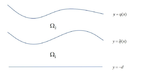
Figure 1: Two-layer stratified water wave consists of $\Omega_{1}$ and $\Omega_{2}$. The internal boundary $\widetilde{\eta}(x)$ represents the pycnoclines. As the water wave passes through $\widetilde{\eta}(x)$ from $\Omega_{1}$ to $\Omega_{2}$, the density jumps discontinuity from $\rho_{1}$ to $\rho_{2}$.

Let $\rho_{i}$ be the density of the flow in $\Omega_{i}$, for $i=1,2$. It should be noted that $\rho_{i}$ are not constants. In this paper, we assume that the density increases with settlement depth, which implies $\rho_{1}>\rho_{2}$. Inspired by Walsh [18], we present the Euler equations of two-layer water wave together with conservation of mass conditions and in continuity condition after traveling wave transformation:

$$\begin{cases}\rho_{i}(u_{i}-c)u_{ix}+\rho_{i}v_{i}u_{iy}=-P_{ix},\\ \rho_{i}(u_{i}-c)v_{ix}+\rho_{i}v_{i}v_{iy}=-P_{iy}-g\rho_{i},\\ (u_{i}-c)\rho_{ix}+v_{i}\rho_{iy}=0,\\ u_{ix}+v_{iy}=0,\end{cases}$$ (2.1)

where $P_{i}(x,y)$ represent the pressure, for $i=1,2$. And the boundary conditions are give by

$$\begin{cases}v_{2}=(u_{2}-c)\eta(x),\quad&\rm{on}\quad y=\eta(x),\\ v_{1}=(u_{1}-c)\widetilde{\eta}(x),\quad&\rm{on}\quad y=\widetilde{\eta}(x),\\ v_{2}=(u_{2}-c)\widetilde{\eta}(x),\quad&\rm{on}\quad y=\widetilde{\eta}(x),\\ v_{1}=0,\quad&\rm{on}\quad y=-d.\end{cases}$$ (2.2)

We assume that the pressure is continuous, which implies

$$\begin{split}P_{2}=P_{atm},\quad&\rm{on}\quad y=\eta(x),\\ P_{1}=P_{2},\quad&\rm{on}\quad y=\widetilde{\eta}(x),\end{split}$$

where $P_{atm}$ represents the atmospheric pressure.
We also make following assumptions to ensure that no stagnation point exists neither in $\Omega_{1}$ and $\Omega_{2}$:

$$u_{i}-c>0,\quad\rm{in}\quad\Omega_{i}.$$

2.2 Equivalent formulations

Inspired by [18], we introduce the stream function $\Psi_{i}(x,y)$ by

$$\Psi_{iy}(x,y)=-\sqrt{\rho_{i}}v,\quad\Psi_{ix}(x,y)=\sqrt{\rho_{i}}(u-c).$$

And the existence of $\Psi_{i}$ is ensure by the $4$-th equation of (2.1).
It is not difficult to find that $\Psi_{i}$ are constants at the boundary. Moreover, we standardize the boundary values of $\Psi_{i}$ by

$$\begin{cases}\Psi_{1}=\Psi_{2}=0,\quad&\rm{on}\quad y=\widetilde{\eta}(x),\\ \Psi_{1}=-p_{1},\quad&\rm{on}\quad y=-d,\\ \Psi_{2}=-p_{2},\quad&\rm{on}\quad y=\eta(x),\end{cases}$$

where $p_{1}=\int_{-d}^{\widetilde{\eta}(x)}\sqrt{\rho_{1}}(u_{1}(x,y)-c)dy$ and $p_{2}=-\int_{\widetilde{\eta}(x)}^{\eta(x)}\sqrt{\rho_{2}}(u_{2}(x,y)-c)dy$ are constants. The level sets of $\Psi_{i}$ will be referred to as the streamlines of the flow.
Moreover, from Bernoulli’s law, we define the energy function as

$$E_{i}=P_{i}+\rho_{i}\frac{(u_{i}-c)^{2}+v_{i}^{2}}{2}+\rho_{i}g(y+d).$$

Note that $E_{i}$ remain constant along streamlines in $\Omega_{i}$, since $(u-c)E_{ix}+vE_{iy}=0.$
Similarly, we obtain that $\rho_{i}$ are also constants along streamlines in $\Omega_{i}.$ Therefore, we rewrite them as $\rho_{i}=\rho_{i}(-\Psi_{i}(x,y)).$ And we assume $\rho^{\prime}_{i}(-\Psi_{i})\leq 0$, which is physically reasonable. Therefore, we transform the first two equations of (2.1) into

$$\begin{cases}\Psi_{iy}\Psi_{ixy}-\Psi_{ix}\Psi_{iyy}=-P_{ix},\\ \Psi_{ix}\Psi_{ixy}-\Psi_{iy}\Psi_{ixx}=-P_{iy}-g\rho_{i}(-\Psi_{i}).\end{cases}$$ (2.3)

Moreover, according to (2.3), we obtain

$$\nabla^{\perp}\Psi_{i}\cdot\nabla(\Delta\Psi_{i}-gy\rho_{i}^{\prime}(-\Psi_{i}))=0,$$

which means that $\Delta\Psi_{i}-gy\rho_{i}^{\prime}(-\Psi_{i})$ and $\Psi_{i}$ are orthogonal. In other words, there exist $\beta_{1}:[-p_{1},0]\to\mathbb{R}$ and $\beta_{2}:[-p_{2},0]\to\mathbb{R}$, s.t.

$$\Delta\Psi_{i}-gy\rho_{i}^{\prime}(-\Psi_{i})=-\beta_{i}(\Psi_{i}).$$

And we assume $\beta_{i}$ decrease as depth increases, that is

$$\beta_{i}^{\prime}<0.$$

Finally, we transform (2.1) and the dynamic boundary conditions above into

$$\begin{cases}&\Delta\Psi_{i}=gy\rho_{i}^{\prime}(-\Psi_{i})-\beta_{i}(\Psi_{i})\quad\rm{in}\quad\Omega_{i},\quad\rm{for}\quad i=1,2,\\ &\frac{|\nabla\Psi_{2}|}{2}+g\rho_{2}(-\Psi_{2})(y+d)=Q_{2}\quad\rm{on}\quad y=\eta(x),\\ &\frac{|\Psi_{1}|^{2}-|\Psi_{2}|^{2}}{2}+g(\rho_{1}(-\Psi_{1})-\rho_{2}(-\Psi_{2}))(y+d)=Q_{1}\quad\rm{on}\quad y=\widetilde{\eta}(x)\\ &\Psi_{1}=\Psi_{2}=0\quad\rm{on}\quad y=\widetilde{\eta}(x),\\ &\Psi_{1}=-p_{1}\quad\rm{on}\quad y=-d,\\ &\Psi_{2}=-p_{2}\quad\rm{on}\quad y=\eta(x),\end{cases}$$ (2.4)

where $Q_{1}$ and $Q_{2}$ are physical parameters.

3 First variational formulation

Following the ideas developed in Chu et al.[3], Chu and Escher [4], Constantin et al. [6], we aim to determine a variational formulation for problem (2.4). We now show that solutions of (2.4) are characterised as critical points of a certain functional.

Let $\Psi_{1p}$, $\Psi_{2p}$, $\widetilde{\eta}_{p}$, $\eta_{p}$ be the disturbance functions of $(\Psi_{1},\Psi_{2},\widetilde{\eta},\eta)$. Set $\mathbb{G}=\{G:\mathbb{R}\to\mathbb{R}\ is\ a\ C^{2}\ function,\ G\ vanishes\ nowhere\}$. Then we obtain that $G$ is a concave or convex function. And for any $F_{i}\in G$, we define

$$(\partial_{2}F_{i}(y,\cdot))^{-1}(p)=gy\rho_{i}^{\prime}(p)-\beta_{i}(-p),\quad p\in\mathbb{R}.$$ (3.1)

For the sake of notational clarity later on, we will denote by $\partial_{1}F_{i}$ and $\partial_{2}F_{i}$ the derivatives of $F_{i}$ with the respect to the first and second variable, respectively; similarly for higher order derivatives. In fact, from this definition it follows that $F_{i}$ is a $\mathbb{C}^{2}$-function. Furthermore, it should be pointed out that $F_{i}$ is only defined up to a function of $y$, a fact that we are going to exploit in the sequel. In the following Theorem, we restrict the perturbations $(\Psi_{1p},\Psi_{2p},\eta_{p},\widetilde{\eta}_{p})$ of $(\Psi_{1},\Psi_{2},\eta,\widetilde{\eta})$ to the subspace

$$\mathbb{P}=\left\{(\Psi_{1p},\Psi_{2p},\widetilde{\eta_{p}},\eta_{p})\in\mathbb{F}:\int_{B}\Psi_{1py}dx=0\ \rm{and}\ \int_{S}\frac{\partial\Psi_{2p}}{\partial n_{2}}dl=0\right\},$$

and prove that $(\Psi_{1},\Psi_{2},\eta,\widetilde{\eta})$ is a critical point of $H$ if and only if $(\Psi_{1},\Psi_{2},\eta,\widetilde{\eta})$ solves (2.4)

Theorem 3.1.

Let $F_{i}$ be defined as in (3.1). Then there exist constants $p_{1},p_{2}\in\mathbb{R}$ such that, $(\Psi_{1},\Psi_{2},\eta,\widetilde{\eta})$ is a critical point of the functional

$$\begin{split}H(\Psi_{1},\Psi_{2},\eta,\widetilde{\eta})=\iint_{\Omega_{1}}[\frac{|\nabla\Psi_{1}|^{2}}{2}+g\rho_{1}(p_{1})(y+d)-(Q_{1}+Q_{2})-F_{1}(y,\Delta\Psi_{1})]dydx\\ +\iint_{\Omega_{2}}[\frac{|\nabla\Psi_{2}|^{2}}{2}+g\rho_{2}(0)(y+d)-Q_{2}-F_{2}(y,\Delta\Psi_{2})]dydx,\end{split}$$

if and only if $(\Psi_{1},\Psi_{2},\eta,\widetilde{\eta})$ solves (2.4).

Proof.

Note that

$$\delta H=\lim_{\epsilon\to 0}\frac{H(\Psi_{1}+\epsilon\Psi_{1p},\Psi_{2}+\epsilon\Psi_{2p},\widetilde{\eta}+\epsilon\widetilde{\eta}_{p},\eta+\epsilon\eta_{p})-H(\Psi_{1},\Psi_{2},\widetilde{\eta},\eta)}{\epsilon},$$

we decompose $\delta H$ into four parts:

$$\delta H=\delta H_{1}+\delta H_{2}+\delta H_{3}+\delta H_{4}.$$ (3.2)

By direct computation, we obtain that

$$\begin{split}\delta H_{1}=-\iint_{\Omega_{1}}[\Psi_{1}+\partial_{2}F_{1}(y,\Delta\Psi_{1})]\Delta\Psi_{1p}dydx\\ -\iint_{\Omega_{2}}[\Psi_{2}+\partial_{2}F_{2}(y,\Delta\Psi_{2})]\Delta\Psi_{2p}dydx,\end{split}$$

$$\delta H_{2}=\int_{S}[\frac{|\nabla\Psi_{2}|^{2}}{2}+g\rho_{2}(p_{1})(y+d)-Q_{2}-F_{2}(y,\Delta\Psi_{2})]\eta_{p}dx,$$

$$\delta H_{3}=\int_{S}\Psi_{2}\cdot\frac{\partial\Psi_{2}}{\partial n_{2}}dl-\int_{\widetilde{S}}\Psi_{2}\frac{\partial\Psi_{2p}}{\partial n_{2}}dl+\int_{\widetilde{S}}\Psi_{1}\frac{\partial\Psi_{1p}}{\partial n_{1}}dl-\int_{B}\Psi_{1}\Psi_{1py}dx,$$

$$\delta H_{4}=\int_{\widetilde{S}}[\frac{|\nabla\Psi_{1}|^{2}-|\nabla\Psi_{2}|^{2}}{2}+g(\rho_{1}(0)-\rho_{2}(0))(y+d)-F_{1}(y,\Delta\Psi_{1})+F_{2}(y,\Delta\Psi_{2})-Q_{1}]\widetilde{\eta}_{p}dx,$$

where $B$ represents the bottom of $\Omega_{1}$, $\widetilde{S}$, $S$ correspond to the upper surface boundary of $\Omega_{1}$, $\Omega_{2}$ respectively and $n_{1}$, $n_{2}$ correspond to the outer normal vectors of $\widetilde{S}$ and $S$ respectively.
According to $(\partial_{2}F_{i}(y,\cdot))^{-1}=gy\rho_{i}^{\prime}(p)-\beta_{i}(-p)$ and the first equation of (2.4), we obtain

$$-\Psi_{i}=\partial_{2}F_{i}(y,\Delta\Psi_{i})\quad\rm{for}\quad i=1,2.$$

Moreover, $\delta H_{1}=0$.
Combining the last three equations of (2.4) with $\int_{B}\Psi_{1py}dx=0,\ \int_{S}\frac{\partial\Psi_{2p}}{\partial n_{2}}dl=0$, we obtain

$$\int_{\widetilde{S}}\Psi_{1}\frac{\partial\Psi_{1p}}{\partial n_{1}}dl=0$$

and

$$\int_{\widetilde{S}}\Psi_{2}\frac{\partial\Psi_{2p}}{\partial n_{1}}dl=0.$$

Therefore, we have

$$-\int_{B}\Psi_{1}\Psi_{1py}dx+\int_{S}\Psi_{2}\frac{\partial\Psi_{2p}}{\partial n_{2}}dl=p_{1}\int_{B}\Psi_{1py}dx-p_{2}\int_{S}\frac{\partial\Psi_{2p}}{\partial n_{2}}dl=0,$$

which implies $\delta H_{3}=0.$
According to the second equation of (2.4), we have

$$\delta H_{2}=\int_{\widetilde{S}}-F_{2}(y,\Delta\Psi_{2})\eta_{p}dx=0,$$

by letting $F_{2}(gy\rho_{2}^{\prime}(-\Psi_{2})-\beta_{2}(\Psi_{2}))=0$ (this is not contradictory to the definition of $F_{2}$).

Similarly, we let $F_{1}(y,\Delta\Psi_{1})=F_{2}(y,\Delta\Psi_{2})$. Then, we obtain

$$\frac{|\nabla\Psi_{1}|^{2}-|\nabla\Psi_{2}|^{2}}{2}+g(\rho_{1}(0)-\rho_{2}(0))(y+d)=Q_{1}\quad\rm{on}\quad y=\widetilde{\eta}(x).$$

Therefore, $\delta H_{4}=0.$

Now we prove that if $\delta H=0$, then $(\Psi_{1},\Psi_{2},\eta,\widetilde{\eta})$ solves (2.4).
(i) Take $\eta_{p}=\widetilde{\eta}_{p}=0$ and let $\Psi_{1p}$, $\Psi_{2p}$ satisfy that

$$\begin{cases}\Psi_{1py}=0\quad\rm{on}\quad B,\\ \frac{\partial\Psi_{1p}}{\partial n_{1}}=0\quad\rm{on}\quad S.\end{cases}$$

and

$$\begin{cases}\frac{\partial\Psi_{2p}}{\partial n_{2}}=0\quad\rm{on}\quad S,\\ \frac{\partial\Psi_{2p}}{\partial n_{1}}=0\quad\rm{on}\quad\widetilde{S}.\end{cases}$$

Then (3.2) is simplified as

$$\iint_{\Omega_{1}}(\Psi_{1}+\partial_{2}F_{1}(y,\Delta\Psi_{1}))\omega_{1p}dydx+\iint_{\Omega_{2}}(\Psi_{2}+\partial_{2}F_{2}(y,\Delta\Psi_{2}))\omega_{2p}dydx=0,$$

where $\omega_{1p}=\Delta\Psi_{1p}$, $\omega_{2p}=\Delta\Psi_{2p}$ are arbitrary functions satisfying

$$\iint_{\Omega_{i}}\omega_{ip}dydx=0,\quad\rm{for}\quad i=1,2.$$

Therefore, there exist $k_{1}$, $k_{2}\in\mathbb{R}$ satisfying

$$\partial_{2}F_{i}(y,\Delta\Psi_{i})=-\Psi_{i}+k_{i},\quad\rm{for}\quad i=1,2.$$ (3.3)

According to the definition of $F_{i}$, we obtain that

$$\Delta(\Psi_{i}-k_{i})=gy\rho_{i}^{\prime}(-\Psi_{i}+k_{i})-\beta_{i}(\Psi_{i}-k_{i}),$$

which meets the first equation of (2.4) (with $\Psi_{i}$ replaced by $\Psi_{i}-k_{i}$). Moreover, we rewrite the expression of $\delta H$ as

$$\begin{split}\delta H=&-\iint_{\Omega_{1}}k_{1}\Delta\Psi_{1p}dydx-\iint_{\Omega_{2}}k_{2}\Delta\Psi_{2p}dydx\\ &+\int_{S}[\frac{|\Psi_{2}|^{2}}{2}+g\rho_{2}(0)(y+d)-Q_{2}-F_{2}(y,\Delta_{2}\Psi_{2})]\eta_{p}dx\\ &+\int_{S}\Psi_{2}\frac{\partial\Psi_{2}p}{\partial n_{2}}dl-\int_{\widetilde{S}}\Psi_{2}\frac{\partial\Psi_{2p}}{\partial n_{1}}dl+\int_{\widetilde{S}}\Psi_{1}\frac{\partial\Psi_{1p}}{\partial n_{1}}dl-\int_{B}\Psi_{1}\Psi_{1py}dx\\ &+\int_{\widetilde{S}}[\frac{|\Psi_{1}|^{2}-|\Psi_{2}|^{2}}{2}+g(\rho_{1}(0)-\rho_{2}(0))(y+d)-F_{1}(y,\Delta\Psi_{1})+F_{2}(y,\Delta\Psi_{2})-Q_{1}]\widetilde{\eta}_{p}dx=0.\end{split}$$ (3.4)

(ii) Take $\eta_{p}=\widetilde{\eta}_{p}=0$ and let

$$\begin{cases}\Delta\Psi_{1p}=0\quad in\quad\Omega_{1},\\ \Psi_{1py}=0\quad\rm{on}\quad B,\\ \frac{\partial\Psi_{1p}}{\partial n_{1}}=f_{1}\quad\rm{on}\quad\widetilde{S},\end{cases}$$

and

$$\begin{cases}\Delta\Psi_{2p}=0\quad\rm{in}\quad\Omega_{2},\\ \frac{\partial\Psi_{2p}}{\partial n_{1}}=f_{2}\quad\rm{on}\quad\widetilde{S},\\ \frac{\partial\Psi_{2p}}{\partial n_{2}}=0\quad\rm{on}\quad S,\end{cases}$$

hold for $\Psi_{1p}$, $\Psi_{2p}$, where $f_{1}$ is an arbitrary smooth functions on $B$ and $f_{2}$ is an arbitrary smooth function on $S$ with

$$\int_{B}f_{1}dx=0,\quad\int_{S}f_{2}dl=0.$$

Then (3.4) is transformed into

$$\int_{\widetilde{S}}\Psi_{2}f_{2}dl-\int_{\widetilde{S}}\Psi_{1}f_{1}dx=0,$$

which implies $\Psi_{1}=k_{1}$, $\Psi_{2}=k_{2}$ on $\widetilde{S}$ with $\Psi_{i}$ replaced by $\Psi_{i}-k_{i}$.

(iii) Take $\eta_{p}=\widetilde{\eta}_{p}=0$, $\Psi_{1p},\Psi_{2p}$ be the solution of following equations:

$$\begin{cases}\Delta\Psi_{1p}=0\quad\rm{in}\quad\Omega_{1},\\ \frac{\partial\Psi_{1p}}{\partial n_{1}}=0\quad\rm{on}\quad\widetilde{S},\\ \Psi_{1yp}=f_{1}\quad\rm{on}\quad B,\end{cases}$$

and

$$\begin{cases}\Delta\Psi_{2p}=0\quad\rm{in}\quad\Omega_{2},\\ \frac{\partial\Psi_{2p}}{\partial n_{1}}=0\quad\rm{on}\quad\widetilde{S},\\ \frac{\partial\Psi_{2p}}{\partial n_{2}}=f_{2}\quad\rm{on}\quad S,\end{cases}$$

where $f_{1}$ is an arbitrary smooth function on $B$ and $f_{2}$ is an arbitrary smooth function on $S$ with

$$\int_{B}f_{1}dx=0,\quad\int_{S}f_{2}dl=0.$$

Therefore, (3.4) is transformed into $\int_{S}\Psi_{2}f_{2}dl-\int_{B}\Psi_{1}f_{1}dx=0$, which implies

$$\begin{cases}\Psi_{1}-k_{1}=-k_{B}\quad\rm{on}\quad B,\\ \Psi_{2}-k_{2}=-k_{S}\quad\rm{on}\quad S.\end{cases}$$ (3.5)

Taking $k_{B}=-p_{1}$ and $k_{S}=-p_{2}$, we obtain the last two equations of (2.4) with $\Psi_{i}$ replaced by $\Psi_{i}-k_{i}$.

(iv) Let $\Psi_{1p}=\Psi_{2p}=0$ and $\eta_{p}$, $\widetilde{\eta}_{p}$ be the arbitrary smooth functions. Therefore (3.4) is transformed into

$$\begin{split}&\int_{S}(\frac{|\nabla\Psi_{2}|^{2}}{2}+g\rho_{2}(p_{1})(y+d)-Q_{2}-F_{2}(y,\Delta\Psi_{2}))\eta_{p}dx\\ &+\int_{\widetilde{S}}(\frac{|\nabla\Psi_{1}|^{2}-|\nabla\Psi_{2}|^{2}}{2}+g(\rho_{1}(0)-\rho_{2}(0))(y+d)+F_{2}(y,\Delta\Psi_{2})-F_{1}(y,\Delta\Psi_{1})-Q_{1})\widetilde{\eta}_{p}dx=0.\end{split}$$

Moreover, we have

$$\begin{cases}\frac{|\nabla\Psi_{2}|^{2}}{2}+g\rho_{2}(p_{1})(y+d)-Q_{2}-F_{2}(y,\Delta\Psi_{2})=0,\\ \frac{|\nabla\Psi_{1}|^{2}-|\nabla\Psi_{2}|^{2}}{2}+g(\rho_{1}(0)-\rho_{2}(0))(y+d)+F_{2}(y,\Delta\Psi_{2})-F_{1}(y,\Delta\Psi_{1})-Q_{1}=0.\end{cases}$$

According to (3.3) and (3.5), we obtain

$$\partial_{2}F_{2}(y,\Delta\Psi_{2})=-k_{S}\quad\rm{on}\quad S,$$

or

$$\partial_{2}F_{2}(\eta(x),g\eta(x)\rho^{\prime}(-k_{S})-\beta(k_{S}))=-k_{S}.$$

From the definition of $F_{2}$, it is only related to $y$. We may therefore require

$$F_{2}(y,gy\rho_{2}^{\prime}(-k_{S})-\beta(k_{S}))=0,\quad y\geq-d.$$

Then $F_{2}(\eta(x),\Delta\Psi_{2}(x,\eta(x))=F_{2}(\eta(x),g\rho^{\prime}(-k_{S})-\beta(k_{S}))=0$, for $-\pi<x<\pi$, which leads to the second equation of (2.4). Similarly, we let $F_{1}(y,\Delta\Psi_{1})=F_{2}(y,\Delta\Psi_{2})$ on $y=\widetilde{\eta}(x)$ to obtain the third equation of (2.4). ∎

4 Second variation

Beginning with a critical point $(\Psi_{1},\Psi_{2},\eta,\widetilde{\eta})\in\mathbb{G}$. A pair of variations of the critical point is denoted by $(\Psi_{1p},\Psi_{2p},\eta_{p},\widetilde{\eta}_{p})\in\mathbb{G}$ and $(\overline{\Psi}_{1p},\overline{\Psi}_{2p},{\overline{\eta}}_{p},{\overline{\widetilde{\eta}}}_{p})\in\mathbb{G}$. We also let $\omega_{i}=\Delta\Psi_{i}$, $\omega_{ip}=\Delta\Psi_{ip}$ and $\overline{\omega}_{ip}=\Delta\overline{\Psi}_{ip}$, for $i=1,2$. Then the second variation of $H$ is calculated in the follow theorem.

Theorem 4.1.

If $(\Psi_{1},\Psi_{2},\eta,\widetilde{\eta})$ is the solution of (2.4), then $\delta^{2}H$ is expressed as

$$\begin{split}\delta^{2}H=&\iint_{\Omega_{1}}[\nabla\overline{\Psi}_{1p}\cdot\nabla\Psi_{1p}-\partial_{22}F_{1}(y,\omega_{1})\omega_{1p}\overline{\omega}_{1p}]dydx+\iint_{\Omega_{2}}[\nabla\overline{\Psi}_{2p}\cdot\nabla\Psi_{2p}-\partial_{22}F_{2}(y,\omega_{2})\omega_{2p}\overline{\omega}_{2p}]dydx\\ &+\int_{\overline{S}}\overline{\Psi}_{2p}\frac{\partial\Psi_{2p}}{\partial n_{1}}dl+\int_{S}\Psi_{2y}\frac{\overline{\Psi}_{2p}}{\partial n_{2}}\eta_{p}dl+\int_{S}\Psi_{2y}\overline{\eta}_{p}\frac{\partial\Psi_{2p}}{\partial n_{2}}dl\\ &-\int_{\widetilde{S}}(\overline{\Psi}_{2p}+\Psi_{2y}\overline{\widetilde{\eta}}_{p})\frac{\partial\Psi_{2p}}{\partial n_{2}}dl+\int_{\widetilde{S}}\Psi_{1y}\overline{\widetilde{\eta}}_{p}\frac{\partial\Psi_{1p}}{\partial_{n_{1}}}dl+\int_{\widetilde{S}}\Psi_{1y}\frac{\partial\overline{\Psi}_{1p}}{\partial{n_{1}}}\widetilde{\eta}_{p}dl-\int_{\widetilde{S}}\Psi_{2y}\frac{\partial\Psi_{2p}}{\partial n_{1}}\widetilde{\eta}_{p}dl\\ &+\int_{S}\{g\rho_{2}(p_{1})+[\frac{1}{2}|\nabla\Psi|^{2}]_{y}\}\eta_{p}\overline{\eta}_{p}dx-\int_{S}\partial_{2}F_{2}(y,\omega_{2})\overline{\omega}_{2p}\eta_{p}dx\\ &-\int_{S}[\partial_{1}F_{2}(y,\omega_{2})+\partial_{2}F_{2}(y,\omega_{2})\omega_{2y}]\eta_{p}\overline{\eta}_{p}dx+\int_{\widetilde{S}}[-\partial_{2}F_{1}(y,\omega_{1})\overline{\omega}_{1p}+\partial_{2}F_{2}(y,\omega_{2})\overline{\omega}_{2p}]\widetilde{\eta}_{p}dx\\ &+\int_{\widetilde{S}}[g(\rho_{1}(0)-\rho_{2}(0))-\partial_{1}F_{1}(y,\omega_{1})-\partial_{2}F(y,\omega_{1})\omega_{1y}+\partial_{1}F_{2}(y,\omega_{2})+\partial_{2}F_{2}(y,\omega_{2})\omega_{2y}]\widetilde{\eta}\overline{\widetilde{\eta}}_{p}dx.\end{split}$$ (4.1)

Proof.

Noting that $\Psi_{i}=-\partial_{2}F_{i}(y,\omega_{1})$, we obtain $\delta^{2}H=\delta^{2}H_{1}+\delta^{2}H_{2}+\delta^{2}H^{3}+\delta^{2}H_{4}$, where

$$\begin{split}\delta^{2}H_{1}=&-\iint_{\Omega_{1}}[\overline{\Psi}_{1p}+\partial_{22}F_{1}(y,\omega_{1})\overline{\omega}_{1p}]\omega_{1p}dydx-\int_{\widetilde{S}}\overline{\eta}_{p}[\Psi_{1}+\partial_{2}F_{1}(y,\omega_{1})]\omega_{1p}dx\\ &+\int_{\widetilde{S}}[\Psi_{2}+\partial_{2}F_{2}(y,\omega_{2})]\omega_{1p}\overline{\widetilde{\eta}}_{p}dx-\int_{S}[\Psi_{2}+\partial_{2}F_{2}(y,\omega_{2})]\omega_{2p}\overline{\eta}_{p}dx\\ &-\iint_{\Omega_{2}}[\overline{\Psi}_{2p}+\partial_{22}F_{2}(y,\omega_{2})\overline{\omega}_{2p}]\omega_{2p}dydx\\ =&-\iint_{\Omega_{1}}[\overline{\Psi}_{1p}+\partial_{22}F_{1}(y,\omega_{1})\overline{\omega}_{1p}]\omega_{1p}dydx-\iint_{\Omega_{2}}[\overline{\Psi}_{2p}+\partial_{22}F_{2}(y,\omega_{2})\overline{\omega}_{2p}]\omega_{2p}dydx\\ =&\iint_{\Omega_{1}}[\nabla\overline{\Psi}_{1p}\cdot\nabla\Psi_{1p}-\partial_{22}F_{1}(y,\omega_{1})\omega_{1p}\overline{\omega}_{1p}]dydx+\iint_{\Omega_{2}}[\nabla\overline{\Psi}_{2p}\cdot\nabla\Psi_{2p}-\partial_{22}F_{2}(y,\omega_{2})\omega_{2p}\overline{\omega}_{2p}]dydx\\ &-\int_{\widetilde{S}}\overline{\Psi}_{1p}\frac{\partial\Psi_{1p}}{\partial n_{1}}dl+\int_{\widetilde{S}}\overline{\Psi}_{2p}\frac{\partial\Psi_{2p}}{\partial n_{1}}dl-\int_{S}\overline{\Psi}_{2p}\frac{\partial\Psi_{2p}}{\partial n_{2}}dl+\int_{B}\overline{\Psi}_{1p}\frac{\partial\Psi_{1p}}{\partial y}dx.\end{split}$$

Noting that $\delta\int_{S}fdl=\int_{S}\delta fdl+\int_{S}f_{y}\delta\eta dl$ and $\delta\int_{\widetilde{S}}fdl=\int_{\widetilde{S}}\delta fdl+\int_{\widetilde{S}}f_{y}\delta\widetilde{\eta}dl$ (see [8]), $\delta^{2}H_{2}$ is given by

$$\begin{split}\delta^{2}H_{2}=&\int_{S}[\Psi_{2x}\overline{\Psi}_{2px}+\Psi_{2y}\Psi_{2py}-\partial_{2}F_{2}(y,\omega_{2})\overline{\omega}_{2p}]\eta_{p}dx\\ &+\int_{S}[\Psi_{2x}\Psi_{2xy}+\Psi_{2y}\Psi_{2yy}+g\rho_{2}(p_{1})-\partial_{1}F_{2}(y,\omega_{2})-\partial_{2}F_{2}(y,\omega_{2})\omega_{2y}]\eta_{p}\overline{\eta}_{p}dx\\ =&\int_{S}\Psi_{2y}\frac{\partial\overline{\Psi}_{2p}}{\partial n_{2}}\eta_{p}dl+\int_{S}\{g\rho_{2}(p_{1})+[\frac{1}{2}|\nabla\Psi_{2}|^{2}]_{y}\}\eta_{p}\overline{\eta}_{p}dx\\ &-\int_{S}\partial_{2}F_{2}(y,\omega_{2})\overline{\omega}_{2p}\eta_{p}dx-\int_{S}[\partial_{1}F_{2}(y,\omega_{2})+\partial_{2}F_{2}(y,\omega_{2})\omega_{2y}]\eta_{p}\overline{\eta}_{p}dx.\end{split}$$

Similarly, the remaining two terms is calculated as follows

$$\begin{split}\delta^{2}H_{3}=&\int_{S}(\overline{\Psi}_{2p}+\Psi_{2y}\overline{\eta}_{p})\frac{\partial\Psi_{2p}}{\partial n_{2}}dl-\int_{\widetilde{S}}(\overline{\Psi}_{2p}+\Psi_{2y}\overline{\widetilde{\eta}}_{p})\frac{\partial{\Psi_{2p}}}{\partial n_{2}}dl\\ &+\int_{\widetilde{S}}(\overline{\Psi}_{1p}+\Psi_{1y}\overline{\widetilde{\eta}}_{p})\frac{\partial{\Psi_{1p}}}{\partial n_{1}}dl-\int_{B}\overline{\Psi}_{1p}\Psi_{1py}dx,\end{split}$$

$$\begin{split}\delta^{2}H_{4}&=\int_{\widetilde{S}}[\Psi_{1x}\overline{\Psi}_{1px}+\Psi_{1y}\overline{\Psi}_{1py}-\partial_{2}F_{1}(y,\omega_{1})\overline{\omega}_{1p}+\partial_{2}F_{2}(y,\omega_{2})\overline{\omega}_{2p}]\widetilde{\eta}_{p}dx\\ &+\int_{\widetilde{S}}[g(\rho_{1}(0)-\rho_{2}(0))-\partial_{1}F_{1}(y,\omega_{1})-\partial_{2}F(y,\omega_{1})\omega_{1y}+\partial_{1}F_{2}(y,\omega_{2})+\partial_{2}F_{2}(y,\omega_{2})\omega_{2y}]\widetilde{\eta}\overline{\widetilde{\eta}}_{p}dx\\ =&\int_{\widetilde{S}}\Psi_{1y}\frac{\partial\overline{\Psi}_{1p}}{\partial n_{1}}\widetilde{\eta}_{p}dl-\int_{\widetilde{S}}\Psi_{2y}\frac{\partial\Psi_{2p}}{\partial n_{1}}\widetilde{\eta}_{p}dl+\int_{\widetilde{S}}[-\partial_{2}F_{1}(y,\omega_{1})\overline{\omega}_{1p}+\partial_{2}F_{2}(y,\omega_{2})\overline{\omega}_{2p}]\widetilde{\eta}_{p}dx\\ &+\int_{\widetilde{S}}[g(\rho_{1}(0)-\rho_{2}(0))-\partial_{1}F_{1}(y,\omega_{1})-\partial_{2}F(y,\omega_{1})\omega_{1y}+\partial_{1}F_{2}(y,\omega_{2})+\partial_{2}F_{2}(y,\omega_{2})\omega_{2y}]\widetilde{\eta}\overline{\widetilde{\eta}}_{p}dx.\end{split}$$

∎

Definition 4.2.

The traveling wave $(\Psi_{1},\Psi_{2},\widetilde{\eta},\eta)$ is linear stable if for any $(\Psi_{1p},\Psi_{2p},\widetilde{\eta}_{p},\eta_{p})\in\mathbb{G}$, the quadratic form $\delta^{2}H$ is nonnegative.

Now we give the quadratic form of $\delta^{2}H$ by taking $(\Psi_{1p},\Psi_{2p},\eta_{p},\widetilde{\eta}_{p})=(\overline{\Psi}_{1p},\overline{\Psi}_{2p},\overline{\eta}_{p},\overline{\widetilde{\eta}}_{p})$ in (4.1).

$$\begin{split}\delta^{2}H=&\iint_{\Omega_{1}}[\nabla{\Psi}_{1p}\cdot\nabla\Psi_{1p}-\partial_{22}F_{1}(y,\omega_{1})|\omega_{1p}|^{2}]dydx+\iint_{\Omega_{2}}[\nabla{\Psi}_{2p}\cdot\nabla\Psi_{2p}-\partial_{22}F_{2}(y,\omega_{2})|\omega_{2p}|^{2}]dydx\\ &+\int_{\overline{S}}\Psi_{2p}\frac{\partial\Psi_{2p}}{\partial n_{1}}dl+\int_{S}\Psi_{2y}\frac{\Psi_{2p}}{\partial n_{2}}\eta_{p}dl+\int_{S}\Psi_{2y}{\eta}_{p}\frac{\partial\Psi_{2p}}{\partial n_{2}}dl\\ &-\int_{\widetilde{S}}(\Psi_{2p}+\Psi_{2y}{\widetilde{\eta}}_{p})\frac{\partial\Psi_{2p}}{\partial n_{2}}dl+\int_{\widetilde{S}}\Psi_{1y}{\widetilde{\eta}}_{p}\frac{\partial\Psi_{1p}}{\partial_{n_{1}}}dl+\int_{\widetilde{S}}\Psi_{1y}\frac{\partial\Psi_{1p}}{\partial{n_{1}}}\widetilde{\eta}_{p}dl-\int_{\widetilde{S}}\Psi_{2y}\frac{\partial\Psi_{2p}}{\partial n_{1}}\widetilde{\eta}_{p}dl\\ &+\int_{S}\{g\rho_{2}(p_{1})+[\frac{1}{2}|\nabla\Psi|^{2}]_{y}\}\eta_{p}^{2}dx-\int_{S}\partial_{2}F_{2}(y,\omega_{2})\omega_{2p}\eta_{p}dx\\ &-\int_{S}[\partial_{1}F_{2}(y,\omega_{2})+\partial_{2}F_{2}(y,\omega_{2})\omega_{2y}]\eta_{p}^{2}dx+\int_{\widetilde{S}}[-\partial_{2}F_{1}(y,\omega_{1}){\omega}_{1p}+\partial_{2}F_{2}(y,\omega_{2})\omega_{2p}]\widetilde{\eta}_{p}dx\\ &+\int_{\widetilde{S}}[g(\rho_{1}(0)-\rho_{2}(0))-\partial_{1}F_{1}(y,\omega_{1})-\partial_{2}F(y,\omega_{1})\omega_{1y}+\partial_{1}F_{2}(y,\omega_{2})+\partial_{2}F_{2}(y,\omega_{2})\omega_{2y}]\widetilde{\eta}{\widetilde{\eta}}_{p}dx.\end{split}$$ (4.2)

Therefore, suitable conditions to ensure (4.1) is nonnegative are necessary for us to obtain the linear stable results.

Theorem 4.3.

If the surface $\eta$ and the interface $\widetilde{\eta}$ are unperturbed and $\partial_{22}F_{i}(y,\omega_{i})<0$ hold for $i=1,2,$, then a classical travelling wave of (2.4) is linearly stable.

We provide the above theorem, which ensure that the traveling wave is linear stable. Since the proof of the theorem is simple, we omit it here. For the study of more sufficiency conditions, we will leave it as the future topic.

References

- [1] F. Cavallini, F. Crisciani, Quasi-geostrophic theory of oceans and atmosphere, Springer 2013 pp. 385.
- [2] R. Chen, S. Walsh, Unique determination of stratified steady water waves from pressure, J. Differential Equations, 264 (2018) 115–133.
- [3] J. Chu, Q. Ding, J. Escher, Variational formulation of rotational steady water waves in two-layer flows, J. Math. Fluid Mech. 23 No. 91 (2021) 17 pp.
- [4] J. Chu, J. Escher, Variational formulations of steady rotational equatorial waves, Adv. Nonlinear Anal. 10 (2021) 534-547.
- [5] J. Chu, L. Wang, Analyticity of rotational traveling gravity two-layer waves, Stud. Appl. Math. 146 (2021) 605–634.
- [6] A. Constantin, D. Sattinger, W. Strauss, Variational formulation for steady water waves with vorticity. J. Fluid Mech., 548 (2006) 151–163.
- [7] A. Constantin, W. Strauss, Exact steady periodic water waves with vorticity, Comm. Pure Appl. Math., 57 (2004) 481–527.
- [8] A. Constantin, W. Strauss, Stability properties of steady water waves with vorticity. Comm. Pure Appl. Math., 60 (2007) 911–950.
- [9] A. Constantin, R. Ivanov, A Hamiltonian approach to wave-current interactions in two-layer fluids, Phys. Fluids, 27 (2015) 086603.
- [10] A. Constantin, R. Ivanov, Equatorial wave-current interactions. Comm. Math. Phys., 370 (2019) 1–48.
- [11] A. Constantin, R. Johnson, The dynamics of waves interacting with the equatorial undercurrent, Geophys. Astrophys. Fluid Dyn., 109 (2015) 311–358.
- [12] M. Dubreil-Jacotin, Sur la détermination rigoureuse des ondes permanentes périodiques d’ampleurs finie. J. Math. Pures Appl., 13 (1934) 217–291.
- [13] J. Escher, A. Matioc, B. Matioc, On stratified steady periodic water waves with linear density distribution and stagnation points, J. Differential Equations, 251 (2011) 2932–2949.
- [14] S. Haziot, Stratified large-amplitude steady periodic water waves with critical layers. Comm. Math. Phys., 381 (2021) 765–797.
- [15] D. Henry, B. Matioc: Global bifurcation of capillary-gravity-stratified water waves. Proc. Roy. Soc. Edinburgh Sect., A 144 (2014) 775–786.
- [16] D. Henry, B. Matioc, On the existence of steady periodic capillary-gravity stratified water waves, Ann. Sc. Norm. Super. Pisa Cl. Sci., 12 (2013) 955–974.
- [17] C. Jackson, Atlas of internal solitary waves, http://www.internalwaveatlas.com/, February 2004.
- [18] S. Walsh, Stratified steady periodic water waves, SIAM J. Math. Anal., 41 (2009) 1054-1105.
- [19] S. Walsh, O. Bühler, J. Shatah, Steady water waves in the presence of wind, SIAM J. Math. Anal., 45 (2013) 2182–2227.
- [20] M. Wheeler, On stratified water waves with critical layers and Coriolis force, Discrete Contin. Dyn. Syst., 39 (2019) 4747–4770.
- [21] F. Xu, F. Li, Y. Zhang, The symmetry of steady stratified periodic gravity water waves. Monatsh. Math., (2023). https://doi.org/10.1007/s00605-023-01904-4.