Self-tuning model predictive control for wake flows

Abstract

This study presents a noise-robust closed-loop control strategy for wake flows employing model predictive control. The proposed control framework involves the autonomous offline selection of hyperparameters, eliminating the need for user interaction. To this purpose, Bayesian optimization maximizes the control performance, adapting to external disturbances, plant model inaccuracies, and actuation constraints. The noise robustness of the control is achieved through sensor data smoothing based on local polynomial regression. The plant model can be identified through either theoretical formulation or using existing data-driven techniques. In this work, we leverage the latter approach, which requires minimal user intervention. The self-tuned control strategy is applied to the control of the wake of the fluidic pinball, with the plant model based solely on aerodynamic force measurements. The closed-loop actuation results in two distinct control mechanisms: boat tailing for drag reduction and stagnation point control for lift stabilization. The control strategy proves to be highly effective even in realistic noise scenarios, despite relying on a plant model based on a reduced number of sensors.

 

1 Introduction

Prediction and control of fluid flows to pursue a specific objective is a highly compelling research area (Gad-el Hak, 2000). Flow control offers wide-ranging practical applications in diverse fields, including vehicle dynamics, aircraft, and marine transportation, meteorology, energy production from water and wind, combustion, and chemical processes, and more (Duriez et al., 2017). The goals of fluid flow control generally encompass, among others, drag reduction, control of separation and transition, lift or mixing enhancement. In recent years, drag reduction has received considerable attention due to its notable impact on the environmental footprint of transportation means (Green, 2003).

In the last decades, active flow control has garnered increasing attention. This technique can be implemented in open-loop and closed-loop configurations. The former involves pre-determining the actuation law irrespective of the system state, thus simplifying its application. Notable examples include wake control of bluff bodies (Blackburn & Henderson, 1999; Cetiner & Rockwell, 2001; Thiria et al., 2006; Parkin et al., 2014) and open-cavity flows (Sipp, 2012; Little et al., 2007; Nagarajan et al., 2018), among others. However, open-loop control’s effectiveness is limited in unstable flow stabilization, responding to changes in the controlled system parameters, or dealing with external disturbances. On the contrary, closed-loop implementations (also referred to as reactive control) involve feeding the control law by the knowledge of the state. This approach offers greater flexibility and adaptability (Brunton & Noack, 2015). Experimental evidence demonstrates the superior performance of closed-loop over open-loop control, see e.g. Pinier et al. (2007) or Shimomura et al. (2020).

The identification of control laws requires adequate knowledge of the system dynamics and its response to control inputs. In fluid dynamics, model-based techniques have traditionally been utilized to obtain this information, proving successful in various scenarios (Kim & Bewley, 2007). Examples of applications include transition delay in spatially evolving wall-bounded flows (Monokrousos et al., 2008; Chevalier et al., 2007; Tol et al., 2019), cavity flow control (Rowley & Williams, 2006; Illingworth et al., 2011), separation control on a low Reynolds number airfoil (Ahuja et al., 2007), wake stabilization of cylinders (Schumm et al., 1994; Gerhard et al., 2003; Tadmor et al., 2011), skin-friction drag reduction (Cortelezzi & Speyer, 1998; Lee et al., 2001; Kim, 2011) and heat transfer control (Castellanos et al., 2022b). However, the identification of efficient analytical control laws faces an important challenge in the presence of complex nonlinear multiscale dynamics.

In recent years, model-free techniques have gained popularity, driven by advancements in hardware and the increasing efficiency of data-driven and machine-learning (ML) algorithms. Examples of model-free techniques include genetic algorithms in jet mixing optimization (Koumoutsakos et al., 2001; Wu et al., 2018), wake flows (Poncet et al., 2005; Raibaudo et al., 2020), separation control (Gautier et al., 2015), and combustion noise (Buche et al., 2002). Reinforcement learning (RL) has also recently gained popularity, with successful applications in the control of bluff body wakes (Rabault et al., 2019; Fan et al., 2020; Castellanos et al., 2022a) and natural convection (Beintema et al., 2020). Despite the encouraging results of such model-free techniques, their effectiveness is limited by the need for large datasets.

Within model-based techniques, model predictive control (MPC) offers interesting features to deal with the challenges of fluid flow control. MPC is based on the idea of receding horizon control. It found application in the industry since the 1980s (Qin & Badgwell, 2003), in particular with extensive use in refineries and the petrochemical industry (Lee, 2011). MPC has demonstrated excellent performance in controlling complex systems with constraints, strong non-linearities, and time delays (Henson, 1998; Allgöwer et al., 2004; Camacho & Alba, 2013; Grüne & Pannek, 2017). Therefore, it is particularly appropriate for complex systems that challenge traditional linear controllers (Corona & De Schutter, 2008). The method requires the identification of a model of the system dynamics capable of predicting its behavior under exogenous inputs. The optimal control is determined through the iterative solution of an optimization problem within a prediction window, aiming to minimize a user-defined cost function that considers the distance of the system state from the control target. Moreover, MPC allows for the straightforward implementation of hard constraints, such as hardware limitations, distinguishing it from classical control approaches. MPC has been successfully applied in the control of complex fluid systems, see e.g. the works of Collis et al. (2000); Bewley et al. (2001); Bieker et al. (2020); Sasaki & Tsubakino (2020); Morton et al. (2018); Peitz et al. (2020). A crucial aspect of MPC implementation is achieving a proper balance among the terms of the loss function. The user needs to select weights (referred to as hyperparameters) for the loss, considering factors like closeness to the target, cost of the action, and other application-tailored constraints. This choice has a clear impact on the final performance. In flow control applications, this process traditionally relies on user experience, which poses the risk of suboptimal choices.

Bayesian optimization (BO) or RL techniques have demonstrated excellent results in hyperparameter tuning, particularly in the fields of autonomous driving and robotics (Edwards et al., 2021; Fröhlich et al., 2022; Bøhn et al., 2023). A comprehensive review in this area can be found in Hewing et al. (2020). However, in the application of nonlinear MPC to flow control, examples are scarce, and the choice of MPC parameters is often guided by trial-error and intuition. This approach risks falling into suboptimal configurations that may not adequately account for the different degrees of fidelity in the terms involved in the loss function. This issue is particularly relevant in fluid mechanics, where the uncertainty in predicting the plant behavior and the measured state/control actions should play a role in the parameter selection process. Unfortunately, an analytical formulation is elusive in most cases.

Moreover, as a closed-loop strategy, the implementation of MPC requires feedback, consisting of time-sampled measurements of a feature of the system to be controlled. In real control scenarios, this sampling is often affected by measurement noise, which can compromise control decision-making. Thus, suitable smoothing techniques are necessary to enhance noise robustness. In time series analysis, a nonparametric statistical technique called local polynomial regression (LPR) proves particularly effective in this task. LPR estimates the regression function of sensor outputs and their time derivatives without assuming any prior information. Applications of LPR for control purposes are described in works such as Steffen et al. (2010) or Ouyang et al. (2018).

In this article, we propose a fully automatic architecture that self-tunes control and optimization process parameters with minimal user input. Our MPC framework adapts to different levels of noise and/or limited state knowledge. The methodology builds upon offline black-box optimization via Bayesian methods for hyperparameter tuning. Furthermore, we discuss the robustness enhancement to noise using an online local polynomial regression. The effectiveness of the control algorithm is evaluated through its application to the control of the wake of the fluidic pinball (Deng et al., 2020) in the chaotic regime. Although not strictly needed, plant identification is also data-driven. In this work, nonlinear system identification is performed using the sparse identification of nonlinear dynamics with control (SINDYc, Brunton et al., 2016b).

The paper is organized as follows. Section 2 provides a description of the methodology, emphasizing the mathematical tools and the MPC framework employed. Additionally, this section includes specific details regarding the chosen test case for illustration purposes. The results of the control application, along with their interpretation are provided in § 3. Finally, the conclusions are discussed in § 4.

2 Methodology

This section presents the backbone of the MPC-based control algorithm, with a detailed description of the mathematical tools involved in it. Figure 1 includes a diagram illustrating all the required steps for its implementation. In addition, algorithm 1 is introduced to give more detail on the procedure.

The main block in the schematics represents the MPC algorithm, following the approach proposed by Kaiser et al. (2018). The main novelty in this module is the robustness enhancement by online filtering with LPR. This is particularly useful when the plant dynamics is modeled with time-delay coordinates or their derivatives. LPR is directly applied to past sensor data for online implementation.

The roadmap suggests several necessary steps before implementing the control. First, a training dataset is generated. The dataset consists of the time series of the state dynamics under different exogenous inputs. This data can be collected using various methods, including simulations or experiments. The system state and exogenous inputs should be defined based on the specific system being controlled. Second, a plant model is defined to predict the system behavior. In this work, we use a data-driven nonlinear system identification. The final step, before the implementation of the control, focuses on tuning the parameters that define the MPC cost function. Control performance is significantly influenced by their selection. The self-tuning of the hyperparameters is the core of our framework. This tuning is carried out using a Bayesian optimization algorithm.

An important aspect of the proposed method is the need for minimal user interaction. Indeed, the two main inputs are the reference setpoint (i.e. the control target), and a cost function for the MPC algorithm. The weight of the different contributions in the cost function will be determined in the MPC-tuning. BO automatically adjusts to different levels of noise and uncertainties. This greatly enhances the usability and adaptability of the framework to different systems.

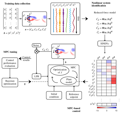
Figure 1: MPC-based control algorithm schematic: dataset generation, creation of the predictive model and parameter tuning. The main block displays the closed-loop MPC scheme, including also LPR to mitigate the effects of sensor measurement noise.

2.1 Self-tuning model predictive control

2.1.1 Model predictive control

This section describes the MPC implementation. It is assumed to have a time-evolving process whose complete description relies on $N_{a}\geq 1$ parameters. These are included in a state vector, denoted at a given instant $t$ as $\boldsymbol{a}\equiv\boldsymbol{a}(t)=\left(a^{1}(t),\ldots,a^{N_{a}}(t)\right)^{\prime}$. The evolution in time of the process can be influenced by the choice of $N_{b}\geq 1$ exogenous parameters. These are included in an input vector $\boldsymbol{b}\equiv\boldsymbol{b}(t)=\left(b^{1}(t),\ldots,b^{N_{b}}(t)\right)^{\prime}$, $\boldsymbol{b}\in\mathcal{B}\subset\mathbb{R}^{N_{b}}$, where $\mathcal{B}$ is the set of allowable inputs. Denoting the time derivative of the state vector with $\dot{\boldsymbol{a}}$, the system dynamics is described by the following set of equations:

$$\begin{array}[]{rcl}\boldsymbol{\dot{a}}&=&f(\boldsymbol{a},\boldsymbol{b})\\ \boldsymbol{a}(0)&=&\boldsymbol{a}_{0},\end{array}$$ (1)

where $\boldsymbol{a}(t_{j})=\boldsymbol{a}_{j}$ and $f$ is the function characterizing the system’s temporal evolution. The process is considered as controlled. This means that for each time $t$, the input vector $\boldsymbol{b}(t)$ can be selected in order to manipulate the system dynamics according to a specific objective. More specifically, the aim is to control $N_{c}\geq 1$ features of the dynamical system, included in the vector $\boldsymbol{c}\equiv\boldsymbol{c}(t)=\left(c^{1}(t),\ldots,c^{N_{c}}(t)\right)^{\prime}$. Note that the vector $\boldsymbol{c}$ is dependent on the system state. In this context, it is assumed that the target features are part of the state vector itself, although this may not always be applicable. The objective is to achieve control over the vector $\boldsymbol{c}$ by ensuring that it closely tends to a desired reference $\boldsymbol{c}_{*}\in\mathbb{R}^{N_{c}}$ over time. MPC can be used for setpoint stabilization, trajectory tracking, or path following (see Raković & Levine, 2018, pp. 169-198), depending on the choice of $\boldsymbol{c}_{*}$.

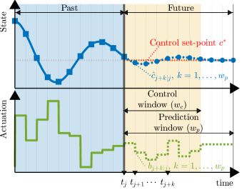
Figure 2: Graphical representation of MPC strategy for stabilizing around a set-point (horizontal dashed line). Past measurements (light-blue-shaded region) depict system state (blue lines with squares) and actuation (green line). The control window $w_{c}$ is shown in orange. Dashed lines indicate future state and actuation predictions. Blue circles represent a discrete sampling of the system state prediction. The continuous formulation allows non-mandatory discrete sampling and step-like actuation can be relaxed.

For the purpose of a control application, $\boldsymbol{a}$, $\boldsymbol{b}$ and $\boldsymbol{c}$ are sampled over a discrete time vector, equispaced with a fixed time interval $T_{s}$. This discrete-time representation is essential to determine how often the exogenous input is updated. The input is assumed to be constant between consecutive timesteps of the control. The implementation of the MPC follows a series of sequential procedures, as can be seen in algorithm 1. An illustration of the process is provided in figure 2.

Firstly, the control process starts from a time instant $t_{j}$, where a measurement $\boldsymbol{s}_{j}$ of the state vector is available. It is assumed that the entire vector of target features is observed. A conditional prediction of the state vector is obtained by a model of the dynamics. This prediction under a given input sequence, referred to as $\boldsymbol{\hat{a}}_{j+k|j}$, is generated within a prediction window $t_{j+k},k=1,\ldots,w_{p}$. Consequently, a prediction of the target features vector $\boldsymbol{\hat{c}}_{j+k|j}$ is obtained.

The optimal input sequence $\{\boldsymbol{b}_{k}^{opt}\}_{k=1}^{w_{c}}$ can be determined in a control window $t_{j+k},k=1,\ldots,w_{c}$, by minimizing a cost function $\mathcal{J}_{MPC}:\mathbb{R}^{N_{b}}\rightarrow\mathbb{R}^{+}$. A common choice for the cost function is

$$\begin{array}[]{ccl}\mathcal{J}_{MPC}(\boldsymbol{b})&=&\sum_{k=0}^{w_{p}}\lVert\boldsymbol{\hat{c}}_{j+k|j}-\boldsymbol{c}_{*}\rVert^{2}_{\mathsfbi{Q}}+\\ &&+\sum_{k=1}^{w_{c}}(\lVert\boldsymbol{b}_{j+k|j}\rVert^{2}_{\mathsfbi{R}_{b}}+\lVert\Delta\boldsymbol{b}_{j+k|j}\rVert^{2}_{\mathsfbi{R}_{\Delta b}}),\end{array}$$ (2)

where $\mathsfbi{Q}\in\mathbb{R}^{{N_{c}}\times{N_{c}}}$ and $\mathsfbi{R}_{b},\mathsfbi{R}_{\Delta b}\in\mathbb{R}^{{N_{b}}\times{N_{b}}}$ are positive and semi-positive definite weight matrices, respectively. In addition, $\lVert\boldsymbol{d}\rVert_{\mathsfbi{M}}^{2}=\boldsymbol{d}^{\prime}\mathsfbi{M}\boldsymbol{d}$ represents the weighted norm of a generic vector $\boldsymbol{d}$ with respect to a symmetric and positive definite matrix $\mathsfbi{M}$, where $\boldsymbol{d}^{\prime}$ denotes the transposition of the vector $\boldsymbol{d}$. The variable $\Delta\boldsymbol{b}_{j+k|j}$, denotes the input variability in time, that is $\boldsymbol{b}_{j+k|j}-\boldsymbol{b}_{j+k-1|j}$. In the definition of the cost function, the errors in state predictions with respect to the reference trajectory, i.e. $\boldsymbol{\hat{c}}_{j+k|j}-\boldsymbol{c}_{*}$, are penalized, as well as the actuation cost and variability. In this paper, the aforementioned weight matrices are assumed to be diagonal, thus:

$$\begin{array}[]{lllll}\mathsfbi{Q}&=&\text{diag(}Q^{1},\ldots,Q^{N_{c}}\text{)},\\ \mathsfbi{R}_{b}&=&\text{diag(}R_{b^{1}},\ldots,R_{b^{N_{b}}}\text{)},\\ \mathsfbi{R}_{\Delta b}&=&\text{diag(}R_{\Delta b^{1}},\ldots,R_{\Delta b^{N_{b}}}\text{)}.\\ \end{array}$$ (3)

Once the optimization problem in (2) is solved, only the first component of the optimal control sequence, $\boldsymbol{b}_{j+1}=\boldsymbol{b}_{1}^{opt}$, is applied. The optimization is then reinitialized and repeated at each subsequent timestep of the control. Generally, the prediction window covers a wider range than the control window ($w_{p}\geq w_{c}$). The control vector is considered constant beyond the end of the control window, as discussed in Kaiser et al. (2018).

Hard constraints on the input vector can readily be incorporated into the optimization process. At each timestep, the optimal problem must guarantee that $\boldsymbol{b}\in\mathcal{B}$, where $\mathcal{B}$ is generally determined by the control hardware. The set of allowable inputs is as follows:

$$\begin{array}[]{rcl}b^{k}_{j}&\in&[b^{k}_{min}\text{ , }b^{k}_{max}]\\ \vspace{0.5cm}\Delta b^{k}_{j}&\in&[\Delta b^{k}_{min}\,\,\,,\Delta b^{k}_{max}]\,\,\,,j=1,\ldots,t\,\,\text{ and }\,\,k=1,\ldots,N_{b},\end{array}$$

being $b^{k}_{j}$ and $\Delta b^{k}_{j}$ the $k^{th}$ control input and input variability component at the $j^{th}$ timestep. The superscripts min and max indicate the minimum and maximum admissible values for the control input and its variability between consecutive timesteps, respectively.

A critical issue of this control technique concerns the choice of parameters. Many of these can be selected based on the physics of the system to be controlled or appropriate control hardware limits, such as the actuation constraints or the control timestep. The selection of parameters involved in equation (3), as well as the length of the prediction/control window, is traditionally tuned by trial and error. In § 2.1.4 we introduce our hyperparameter self-tuning procedure.

2.1.2 Nonlinear system identification

The optimization loop of MPC requires an accurate plant model for predicting the system’s dynamics. The choice of the predictive model typically involves a trade-off between accuracy and computational complexity. In this work, we adopt a data-driven sparsity-promoting technique. The framework was illustrated in the work by Brunton et al. (2016a) and later applied in MPC by Kaiser et al. (2018) for a variety of nonlinear dynamical systems. It must be remarked that the self-tuning framework proposed here can easily be adapted to accommodate a different plant model, either analytical or data-driven, including deep-learning models.

SINDy is a method that identifies a system of ordinary differential equations describing the dynamical system. In particular, the version described in this work corresponds to the extension of the SINDy model with exogenous input (SINDYc, Brunton et al., 2016b). Considering a system of ordinary differential equations such as the one shown in (1), SINDYc derives an analytical expression of $f$ from data. This process requires a dataset comprising the time series of the state vector $\boldsymbol{a}$ and the exogenous input $\boldsymbol{b}$. This method is based on the idea that most physical systems can be characterized by only a few relevant terms, resulting in governing equations that are sparse in a high-dimensional nonlinear function space. The resulting sparse model identification aims to find a balance between model complexity and accuracy, preventing overfitting of the model to the data.

To derive an expression of the function $f$ from data, a discrete sampling is performed on a time vector, yielding $r$ snapshots at time instances $t_{i},i=1,\ldots,r$ for the state vector $\boldsymbol{a}_{i}=\boldsymbol{a}(t_{i})$, its time derivative $\dot{\boldsymbol{a}}_{i}=\dot{\boldsymbol{a}}(t_{i})$, and the input signal $\boldsymbol{b}_{i}=\boldsymbol{b}(t_{i})$. The data obtained are arranged into three matrices $\mathsfbi{A}\in\mathbb{R}^{r\times N_{a}}$, $\dot{\mathsfbi{A}}\in\mathbb{R}^{r\times N_{a}}$ and $\mathsfbi{B}\in\mathbb{R}^{r\times N_{b}}$:

$$\begin{array}[]{rcl}\mathsfbi{A}&=&\left(\boldsymbol{a}_{1}\,,\,\ldots\,,\,\boldsymbol{a}_{r}\right)^{\prime},\vspace{0.1cm}\\ \dot{\mathsfbi{A}}&=&\left(\boldsymbol{\dot{a}}_{1}\,,\,\ldots\,,\,\boldsymbol{\dot{a}}_{r}\right)^{\prime},\vspace{0.1cm}\\ \mathsfbi{B}&=&\left(\boldsymbol{b}_{1}\,,\,\ldots\,,\,\boldsymbol{b}_{r}\right)^{\prime}.\vspace{0.1cm}\\ \end{array}$$ (4)

A library of functions $\boldsymbol{\Theta}$ is then set as:

$$\begin{array}[]{cl}\boldsymbol{\Theta}(\mathsfbi{A},\mathsfbi{B})=&(\mathsfbi{1}_{r},\,\mathsfbi{A},\,\mathsfbi{B},\,\left((\mathsfbi{A}_{1\bullet}\otimes\mathsfbi{A}_{1\bullet})^{\prime},\ldots,(\mathsfbi{A}_{r\bullet}\otimes\mathsfbi{A}_{r\bullet})^{\prime}\right)^{\prime},\\ &\left((\mathsfbi{A}_{1\bullet}\otimes\mathsfbi{B}_{1\bullet})^{\prime},\ldots,(\mathsfbi{A}_{r\bullet}\otimes\mathsfbi{B}_{r\bullet})^{\prime}\right)^{\prime}\\ &\left((\mathsfbi{B}_{1\bullet}\otimes\mathsfbi{B}_{1\bullet})^{\prime},\ldots,(\mathsfbi{B}_{r\bullet}\otimes\mathsfbi{B}_{r\bullet})^{\prime}\right)^{\prime},\ldots),\end{array}$$ (5)

where $\mathsfbi{1}_{r}$ is a column vector of $r$ ones, $\mathsfbi{A}_{i\bullet}$ denotes the $i^{th}$ row of the matrix $\mathsfbi{A}$ and $\mathsfbi{H}\otimes\mathsfbi{K}$ denotes the Kronecker products of $\mathsfbi{H}$ and $\mathsfbi{K}$. The choice of functions to be included in the library is typically made by the user. This procedure is often guided by experience and prior knowledge about the dynamics of the system to be controlled. This issue introduces some limitations that are later discussed in §4.

The system data can be then assumed to be generated from the following model:

$$\dot{\mathsfbi{A}}=\boldsymbol{\Theta}(\mathsfbi{A},\mathsfbi{B})\boldsymbol{\Xi}.$$

$\boldsymbol{\Xi}=\left(\boldsymbol{\xi}^{1},\ldots,\boldsymbol{\xi}^{N_{a}}\right)$ represents the matrix whose rows are vectors of coefficients determining which terms of the right-hand side are active in the dynamics of the $k^{th}$ state vector component. This matrix is sparse for many of the dynamical systems considered. It can be obtained by solving the optimization problem:

$$\hat{\boldsymbol{\xi}}^{k}=\underset{\boldsymbol{\xi}^{k}}{argmin}\left\{\frac{1}{2}\lVert\dot{\mathsfbi{A}}_{\bullet k}-\boldsymbol{\Theta}(\mathsfbi{A},\mathsfbi{B})\boldsymbol{\xi}^{k}\rVert^{2}_{2}\,+\,\lambda\lVert\boldsymbol{\xi}^{k}\rVert_{1}\right\},$$ (6)

where $\lambda$ is called sparsity-promoting coefficient, $\mathsfbi{A}_{\bullet k}$ denotes the $k^{th}$ column of the matrix $\mathsfbi{A}$. $\lVert\cdot\rVert_{1}$ and $\lVert\cdot\rVert_{2}$ are the $L_{1}$ and $L_{2}$ norms, respectively. It must be remarked that $\lambda$ must be optimized to reach a compromise between parsimony and accuracy. Nonetheless, since this block of the MPC framework can easily be replaced by other strategies, $\lambda$ will not be included in the self-tuning optimization illustrated in § 2.1.4.

Finally, the system can be described by:

$$\dot{\boldsymbol{a}}^{k}=\boldsymbol{\Theta}(\boldsymbol{a},\boldsymbol{b})\hat{\boldsymbol{\xi}}^{k},\,\,\,\,k=1,\ldots,N_{a},$$ (7)

where in this case $\boldsymbol{\Theta}(\boldsymbol{a},\boldsymbol{b})$ is a vector that takes into account the same functions included in the library in (5). The SINDYc-based model is utilized to make predictions of the dynamics involved in the control process starting from a specific state’s initial condition. The steps described in this section to obtain the plant model are also condensed in the nonlinear system identification step in algorithm 1.

2.1.3 Local Polynomial Regression

Effectively estimating system dynamics is crucial for various control techniques, particularly in MPC, where sensor feedback is utilized to make informed decisions. The accuracy of system dynamics estimation becomes paramount in MPC as it relies on sensor information to predict the behavior of the controlled system. However, the presence of noise can hinder accurate estimation, necessitating the implementation of noise mitigation techniques.

This challenge falls within the broader context of time series analysis, as sensor outputs represent discrete samples over time of a process variable. To address measurement noise, LPR emerges as a robust, accurate, and cost-effective nonparametric smoothing technique. Applying LPR to sensor output data enhances the reliability and accuracy of estimating the current state of the system under varying noise conditions. In this section, we provide a succinct overview of the formulation of LPR. The notation convention involves denoting random variables with capital letters, while deterministic values are represented in lowercase.

The objective is to predict or explain the response $S$ (sensor output) using the predictor $T$ (time) from a sample $\left\{(T_{i},S_{i})\right\}_{j=1}^{n}$ using the following regression model:

$$S_{j}=m(T_{j})+\sigma(T_{j})\epsilon_{j},$$ (8)

where $m$ is the regression function, $\{\epsilon_{j}\}_{j=1}^{n}$, are zero mean and unit variance random variables and $\sigma^{2}$ is the point variance. For simplicity, it is assumed that the model is homoscedastic, i.e. that the variance is constant. From a practical point of view, $\sigma$ also represents the measurement of noise intensity.

The reason why LPR is used in this context is that it allows for a fast joint estimation of the regression function and its derivatives without making any prior. By making only a few regularity assumptions, it is characterized by a good flexibility that allows to model complex relations beyond a parametric form. The working principle of the LPR is to approximate the regression function locally by a polynomial of order $p$, performing a weighted least squares regression using data only around the point of interest.

It is assumed that the regression functions admit derivatives up to the order $p+1$ and thus that it can be expanded in Taylor’s series. For close time instants $t$ and $T_{j}$ the unknown regression function can be approximated by a polynomial of order $p$, then

$$m(T_{j})\approx\sum_{i=0}^{p}\frac{m^{(i)}(t)}{i!}(T_{j}-t)^{i}\equiv\sum_{i=0}^{p}\beta_{i}(T_{j}-t)^{i},$$

The vector of parameters $\boldsymbol{\beta}=(\beta_{0},\ldots,\beta_{p})^{\prime}$ can be estimated by solving the minimization problem:

$$\boldsymbol{\hat{\beta}}=\underset{\boldsymbol{\beta}}{\text{ arg min }}\sum_{j=1}^{n}\{S_{j}-\sum_{i=0}^{p}\beta_{i}(T_{j}-t)^{i}\}^{2}K_{h}(T_{j}-t),$$ (9)

where $h$ is the bandwidth determining the size of the local neighborhood (also called smoothing parameter) and $K_{h}(t)=\frac{1}{h}K(\frac{t}{h})$ with $K$ a kernel function assigning the weights to each observation. Once the vector $\hat{\boldsymbol{\beta}}$ has been obtained, an estimator of the $q^{th}$ derivative of the regression function is

$$\hat{m}^{(q)}(t)=q!\hat{\beta}_{q}.$$

The solution of the optimization in (9) is simplified when the methodology is presented in matrix form. To that end, $\mathsfbi{T}\in\mathbb{R}^{n\times(p+1)}$ is the design matrix

$$\mathsfbi{T}=\begin{pmatrix}1&(T_{1}-t)&\ldots&(T_{1}-t)^{p}\\ \vdots&\vdots&&\vdots\\ 1&(T_{n}-t)&\ldots&(T_{n}-t)^{p}\end{pmatrix}$$

while the vector of responses is $\boldsymbol{S}=(S_{1},\ldots,S_{n})^{\prime}$ and $\mathsfbi{W}=\text{diag}(K_{h}(T_{1}-t),\ldots,K_{h}(T_{n}-t))$. According to this notation and assuming the invertibility of $\mathsfbi{T}^{\prime}\mathsfbi{W}\mathsfbi{T}$, the weighted least squares solution of the minimization problem expressed in (9) is

$$\boldsymbol{\hat{\beta}}=(\mathsfbi{T}^{\prime}\mathsfbi{W}\mathsfbi{T})^{-1}\mathsfbi{T}^{\prime}\mathsfbi{W}\boldsymbol{S}$$

and thus the estimator of the local polynomial is:

$$\hat{m}(t)=\boldsymbol{e}_{1}^{\prime}(\mathsfbi{T}^{\prime}\mathsfbi{W}\mathsfbi{T})^{-1}\mathsfbi{T}^{\prime}\mathsfbi{W}\boldsymbol{S}=\sum_{j=1}^{n}W_{j}^{p}(t)S_{j},$$

being $\boldsymbol{e}_{k}\in\mathbb{R}^{(p+1)\times 1}$ a vector having $1$ in the $k^{th}$ entry and zero elsewhere and $W_{j}^{p}(t)=\boldsymbol{e}_{1}^{\prime}(\mathsfbi{T}^{\prime}\mathsfbi{W}\mathsfbi{T})^{-1}\mathsfbi{T}^{\prime}\mathsfbi{W}\boldsymbol{e}_{j}$.

The critical element that determines the degree of smoothing in LPR is the size of the local neighborhood. The selection of $h$ determines the accuracy of the estimation of the regression function: too large values lead to a large bias in the regression, while too small values increase the variance. Its choice is generically the result of a trade-off between the variance and the estimation bias of the regression function. There are several methods to select the bandwidth to be used for LPR. One possible approach is to choose between a global bandwidth, which is common to the entire domain and is optimal for the entire range of data, or a local bandwidth that depends on the covariate and is therefore optimal at each point of the regression function estimation. The latter would allow for more flexibility in estimating inhomogeneous regression functions. However, in the proposed framework, a global bandwidth was chosen due to its simplicity and, more importantly, its reduced computational cost. In the presented approach, the global bandwidth is chosen using the leave-one-out-cross-validation (LOOCV) methodology. Specifically, this parameter corresponds to the one that minimizes the following expression:

$$\sum_{j=1}^{n}\left(S_{j}-\hat{m}_{h,-j}(T_{j})\right)^{2},$$

where $\hat{m}_{h,-j}(T_{j})$ denotes the estimation of the regression function while excluding the $j^{th}$ term. For further information regarding the optimal bandwidth selection see the works of Wand & Jones (1994) and Fan & Gijbels (1996). Additionally, there exist other methodologies that utilize machine learning techniques to select the local bandwidth such as in Giordano & Parrella (2008) where neural networks are used.

Once the smoothing parameter has been set, it remains to choose the weighting function and the degree of the local polynomial, although these two have a minor influence on the performance of the LPR estimation. A common choice for the first is the Epanechnikov kernel. As for the degree of the local polynomial, there is a general pattern of increasing variability according to which, to estimate $m^{(q)}(t)$, the lowest odd order is recommended, i.e. $p=q+1$ or occasionally $p=q+3$ (Fan & Gijbels, 1996).

It is also worth noting that due to asymmetric estimation within the control algorithm, boundary effects arise, leading to a bias in the estimation at the edge. These effects, discussed in more detail in Fan & Gijbels (1996), disappear when using local linear regression ($p=1$).

2.1.4 Hyperparameter automatic tuning with Bayesian optimization

MPC relies on a specific set of hyperparameters to precisely define the cost function in (2) for the selection of the optimal action over the control window. A new functional, based on the global performance of the control, is defined. Bayesian optimization is employed to find the hyperparameter vector that maximizes the control performance. By adopting this approach, a more efficient and effective MPC-based control framework may be achieved. The hyperparameters are indeed adapted to different conditions of measurement noise and/or model uncertainty by the BO process. This proposed framework is practically independent of the user.

The parameters under consideration include i) the components of the weight matrices, as presented in (3), which penalize errors of the state vector with respect to the control target trajectories, input cost, and input time variability and ii) the length of the control/prediction windows, assumed equal for simplicity. All aforementioned control parameters are included in a single vector denoted as $\boldsymbol{\eta}\in\mathbb{R}^{N_{\boldsymbol{\eta}}}$, where $N_{\boldsymbol{\eta}}=2N_{b}+N_{c}+1$. A further reduction in the number of control parameters can be also considered by imposing that the components of $\mathsfbi{R}_{b}$ and $\mathsfbi{R}_{\Delta b}$ related to the rear cylinders of the fluidic pinball are identical under a flow symmetry argument, as in Bieker et al. (2020). Therefore, in this case it is stated that ${R}_{b^{2}}={R}_{b^{3}}={R}_{b^{2,3}}$ and ${R}_{\Delta b^{2}}={R}_{\Delta b^{3}}={R}_{\Delta b^{2,3}}$ and the total number of parameters is reduced to $N_{\boldsymbol{\eta}}=2(N_{b}-1)+N_{c}+1$. Section 3 also provides several results that justify this choice.

Note that control results depend on the selection of the vector $\boldsymbol{\eta}$. Consequently, an offline optimization process can be implemented to select the optimal value of $\boldsymbol{\eta}$, which maximizes the control performance. Consider using a specific realization of the hyperparameter vector $\boldsymbol{\eta}$ to control the system. The state vector measure is indirectly dependent on the choice of hyperparameter vector and is denoted here by $\tilde{\boldsymbol{s}}(\boldsymbol{\eta})$. By running the control on a discrete-time vector of $n_{BO}$ timesteps, the cost function can be defined as follows:

$$\mathcal{J}_{BO}(\boldsymbol{\eta})=\frac{1}{n_{BO}}\sum_{k=1}^{N_{c}}\sum_{j=1}^{n_{BO}}\left(\tilde{s}^{k}_{j}(\boldsymbol{\eta})-c^{k}_{*}\right)^{2}.$$ (10)

Note that the user selects the target to be optimized, specified by the cost function $\mathcal{J}_{BO}$. In addition, in absence of measurement noise, $\tilde{\boldsymbol{s}}(\boldsymbol{\eta})$ is the ideal measure of the target feature vector. Otherwise, the LPR technique is applied to the state vector measure. In this study, the parameters are optimized to minimize the quadratic error between the controlled variables and the user-defined target. Thus, the optimal hyperparameter vector can be obtained by solving the problem

$$\begin{array}[]{rl}\boldsymbol{\eta}_{opt}=\underset{\boldsymbol{\eta}\in H}{\text{arg min}}&\mathcal{J}_{BO}(\boldsymbol{\eta}),\\ \end{array}$$ (11)

where $H\subset\mathbb{R}^{N_{\boldsymbol{\eta}}}$ is the search domain. Solving the optimization in (LABEL:Eqn:BOproblem) is computationally costly due to the expensive sampling of the black-box cost function $\mathcal{J}_{BO}$. Each sample of $\mathcal{J}_{BO}$ is obtained via application of the MPC-based control over $n_{BO}$ timesteps. In this framework, BO serves as an efficient method to address this problem, offering an algorithm to search the minimum of the function with a high guarantee of avoiding local minima and characterized by rapid convergence. Indeed, BO has shown to be an efficient strategy particularly when $N_{\boldsymbol{\eta}}\leq 20$ and the search domain $H$ is a hyper-rectangle, that is $H=\{\boldsymbol{\eta}\in\mathbb{R}^{N_{\boldsymbol{\eta}}}|\eta^{i}\in[\eta^{i}_{min},\eta^{i}_{max}]\subset\mathbb{R}\,,\eta^{i}_{min}<\eta^{i}_{max}\,,i=1,\ldots,N_{\boldsymbol{\eta}}\}$, where $\boldsymbol{\eta}_{min}$ and $\boldsymbol{\eta}_{max}$ are the lower and upper bound vectors of the hyper-rectangle, respectively.

In order to find the minimum of the unknown objective function, BO employs an iterative approach, as shown in the MPC-tuning step of algorithm 1. It utilizes a probabilistic model, typically a Gaussian process (GP), to estimate the behavior of the objective function. At each iteration, the probabilistic model incorporates available data points to make predictions about the function behavior at unexplored points in the search space. Simultaneously, an acquisition process guides the samplings by suggesting the optimal locations in order to discover the minimum point. A specific function (called acquisition function) is set to balance exploration, by directing attention to less-explored areas of the search domain, and exploitation, by concentrating on regions near potential minimum points. Finally, the BO iterations continue until a stopping criterion is met, such as reaching a maximum number of iterations or achieving convergence in the search for the minimum. Thus, denoting as $\alpha(\boldsymbol{\eta})$ the acquisition function selected, the point where to sample next in the iterative approach, that is $\boldsymbol{\eta}^{+}$, can be obtained by solving

$$\boldsymbol{\eta}^{+}=\underset{\boldsymbol{\eta}\in H}{\text{arg max}}\,\,\,\alpha(\boldsymbol{\eta}).$$

The expected improvement (EI) is used as an acquisition function (Snoek et al., 2012), which evaluates the potential improvement over the current best solution.

The subsequent discussion will center on the probabilistic model utilized in Bayesian optimization. Specifically, a prior distribution, which corresponds to a multivariate Gaussian distribution, is employed. Consider the situation where problem (LABEL:Eqn:BOproblem) is tackled using Bayesian optimization. A Gaussian process regression is required for the functional $\mathcal{J}_{BO}$ based on the available observations of the function up to the given iteration.

Since $\mathcal{J}_{BO}$ is a Gaussian process, for any collection of $D$ points, included in $\boldsymbol{\Xi}=\left(\boldsymbol{\eta}_{1},\ldots,\boldsymbol{\eta}_{D}\right)^{\prime}$, then the vector of function samplings at these points, denoted as $\boldsymbol{J}=\left(\mathcal{J}_{BO}(\boldsymbol{\eta}_{1}),\ldots,\mathcal{J}_{BO}(\boldsymbol{\eta}_{D})\right)^{\prime}$ is multivariate-Gaussian-distributed, then:

$$\boldsymbol{J}\sim\mathcal{N}_{D}(\boldsymbol{\mu},\mathsfbi{K})$$

being $\boldsymbol{\mu}=\left(\mu(\boldsymbol{\eta}_{1}),\ldots,\mu(\boldsymbol{\eta}_{D})\right)^{\prime}$ the mean vector and $\mathsfbi{K}$ the covariance matrix whose $ij^{th}$ component is $K_{ij}=k(\boldsymbol{\eta}_{i},\boldsymbol{\eta}_{j})$, with $\mu$ a mean function and $k$ a positive definite kernel function. For simplicity, the mean function is assumed to be null.

In order to make a prediction of the value of the unknown function at a new point of interest $\boldsymbol{\eta}_{*}$, denoted as $\mathcal{J}_{BO_{*}}$, conditioned on the values of the function already observed, and included in the vector $\boldsymbol{J}$, the joint multivariate Gaussian distribution can be considered:

$$\begin{pmatrix}\boldsymbol{J}\\ \mathcal{J}_{BO_{*}}\end{pmatrix}\sim\mathcal{N}_{D+1}\left(\boldsymbol{0},\begin{pmatrix}\mathsfbi{K}&\boldsymbol{k}_{*}\\ \boldsymbol{k}^{\prime}_{*}&k_{**}\end{pmatrix}\right)$$

where $k_{**}=k(\boldsymbol{\eta}^{*},\boldsymbol{\eta}^{*})$, and the vector $\boldsymbol{k}_{*}=\left(k(\boldsymbol{\eta}_{1},\boldsymbol{\eta}_{*}),\ldots,k(\boldsymbol{\eta}_{D},\boldsymbol{\eta}_{*})\right)^{\prime}$. This equation describes how the samples $\boldsymbol{J}$ at the locations $\boldsymbol{\Xi}$ correlate with the sample of interest $\mathcal{J}_{BO_{*}}$, whose conditional distribution is:

$$\mathcal{J}_{BO_{*}}|\boldsymbol{\eta}_{*},\boldsymbol{\Xi},\boldsymbol{J}\sim\mathcal{N}\left(\mu_{*}\,,\,\sigma_{*}^{2}\right)$$ (12)

with mean $\mu_{*}=\boldsymbol{k}^{\prime}_{*}\boldsymbol{K}^{-1}\boldsymbol{J}$ and variance $\sigma_{*}^{2}=\left(k_{**}-\boldsymbol{k}^{\prime}_{*}\boldsymbol{K}^{-1}\boldsymbol{k}_{*}\right)^{2}$. Equation (12) provides the posterior distribution of the unknown function at the new point where the sample has to be performed. It then furnishes the surrogate model used to describe the function $\mathcal{J}_{BO}$ in the domain for the search of the minimum point.

2.2 The fluidic pinball

The proposed framework is tested on the control of the two-dimensional viscous incompressible flow around a three-cylinder configuration, commonly referred to as fluidic pinball (Pastur et al., 2019; Deng et al., 2020, 2022). The fluidic pinball was chosen because it represents a suitable multiple input multiple output system benchmark for flow controllers.

A representation of the fluidic pinball can be seen in figure 3. The three cylinders have identical diameters $D=2R$, and their geometric centers are placed at the vertices of an equilateral triangle of side $3R$. The centers are symmetrically positioned with respect to the direction of the main flow. The leftmost vertex of the triangle points upstream while the rightmost side is orthogonal to the flow direction. The freestream has a constant velocity equal to $U_{\infty}$. The cylinders of the fluidic pinball, denoted here with $1$ (front), $2$ (top), and $3$ (bottom), can rotate independently around their axes (orthogonal to the plane of the flow) with tangential velocity $b^{1}$, $b^{2}$ and $b^{3}$, respectively.

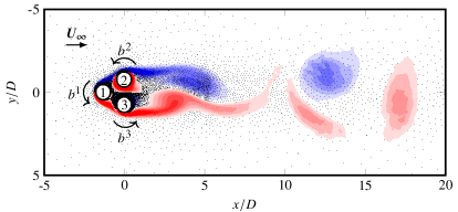
Figure 3: Domain of the incompressible two-dimensional DNS of the flow around fluidic pinball. Front, top and bottom cylinders are labeled as $1$, $2$, and $3$, respectively. The rotational velocities of the cylinders are $b^{1}$, $b^{2}$, and $b^{3}$. The arrows indicate positive (counterclockwise) rotations. The background shows the $8633$ nodes grid used for the DNS. The contour colors indicate the out-of-plane vorticity.

The dynamics of the wake past the fluidic pinball is obtained through a two-dimensional direct numerical simulation (DNS) with the code developed by Noack & Morzyński (2017). The flow is described in a Cartesian reference system in which the $x$ and $y$ axes are in the streamwise and crosswise directions, respectively. The center of the Cartesian reference system coincides with the mid-point of the rightmost bottom and top cylinder and the computational domain, that is $\Omega$, is bounded in $(-5,20)\times(-5,5)$. The position in the reference system is then described by the vector $\boldsymbol{x}=(x,y)=x\boldsymbol{e_{1}}+y\boldsymbol{e_{2}}$, where $\boldsymbol{e_{1}}$ and $\boldsymbol{e_{2}}$ are respectively the unit vectors in the directions of the $x$ and $y$ axes and the velocity vector is assumed to be $\boldsymbol{u}=(u,v)$. The constant density is denoted by $\rho$, the kinematic viscosity of the fluid by $\nu$. All quantities used in the discussion are assumed non-dimensionalized with cylinder diameter, freestream velocity, and fluid density. The Reynolds number is defined as $\Rey_{D}=\frac{U_{\infty}D}{\nu}$. A value of $\Rey_{D}=150$ is adopted, which is sufficiently large to ensure a chaotic behavior, although still laminar. The 2D solver has already been used in previous work at this same $\Rey_{D}$ (Wang et al., 2023). The boundary conditions comprise a far field condition ($\boldsymbol{u}=U_{\infty}\boldsymbol{e_{1}}$) in the upper and lower edges, a stress-free one in the outflow edge, and a no slip-condition on the cylinder walls, which in the absence of forcing becomes $\boldsymbol{u}=0$.

The DNS allows forcing by independent rotation of the cylinders. To this purpose, a velocity with module $|b^{i}|$ is imposed at the cylinder surface. Positive values of $b^{i}$ are associated with counterclockwise rotations of the cylinders. In the remainder of the paper, a reference timescale is set as the convective unit ($c.u.$), i.e. the timescale based on the freestream velocity and the cylinder diameter. The lift coefficient is defined as $C_{l}=\frac{2F_{l}}{\rho U_{\infty}^{2}D}$, being $F_{l}$ the total lift force applied to the cylinders in the direction of $y$-axis and the same quantity is applied in the scaling of $F_{d}$, force applied to the cylinders in direction of $x$-axis, to obtain the total drag coefficient $C_{d}$. The DNS uses a grid of 8633 vertices and 4225 triangles accounting for both accuracy and computational speed. A preliminary grid convergence study at $\Rey_{D}=150$ identified this as sufficient resolution for errors of up to $3\%$ in the free case and $\approx 4\%$ in the actuated case in terms of drag and lift.

2.3 The control approach

The aim of the control is to achieve a reduction in the overall drag coefficient of the fluidic pinball, while also controlling the lift coefficient so that the latter has reduced oscillations with a zero average value. The vector of target features is therefore composed only of the total lift and drag coefficients, $\boldsymbol{c}=(C_{d},C_{l})^{\prime}$. The target vector is thus composed of null components $\boldsymbol{c_{*}}=(0,0)^{\prime}$. Since the cost function in (2) is quadratic, a null target vector will penalize both mean values of $C_{l}$ and $C_{d}$ and their oscillations.

To this purpose, the tangential velocities of the three cylinders are tuned respecting the implementation limits, here chosen equal to $b^{i}\in[-1,1]$ and $\Delta b^{i}\in[-4,4]$ $,\forall i=1,2,3$. The model plant has a state vector composed by $C_{d}$ and $C_{l}$ and their time derivatives, respectively $\dot{C_{d}}$ and $\dot{C_{l}}$ (i.e. $\boldsymbol{a}=(C_{d},C_{l},\dot{C_{d}},\dot{C_{l}})^{\prime}$). A state vector based solely on global variables does not require adding intrusive probes for flow estimation. Similar state vector choices that incorporate aerodynamic force coefficients and temporal derivatives are made in works Nair et al. (2019) and Loiseau et al. (2018). While this approach is often effective in separated flows, it might be challenged at higher $\Rey$ flows and of unfeasible application in other flow configurations.

Feedback to the control involves measurement of drag and lift forces, so at each time instant $t_{j}$, it is considered $\boldsymbol{s}_{j}=\boldsymbol{c}_{j}$. This approach also facilitates a reduction in the complexity of the predictive model, thereby speeding up the control process. Indeed, a compact state vector is particularly desirable to reduce the computational cost of the iterative optimization problem over receding horizons of MPC.

In the present work, noise in lift and drag measurement is also considered. Under this assumption, the model in equation (8) is applied. The noise intensity $\sigma$ is assumed to be constant over time and given as a percentage of the full-scale measured drag and lift coefficients in conditions without actuation. Therefore in the case of measurement noise in the sensors, the response variable to which the LPR is applied corresponds to the measurements of the drag and lift coefficients of the fluidic pinball. The LPR enables us to obtain estimates of their regression function in output from the sensors but also of their time derivatives, allowing us to use this information as control feedback.

The MPC-optimization problem is solved every control timestep (so every $T_{s}$) to update the exogenous control input. During the time between two consecutive samples, the control input to the system remains constant. Thus, the sampling timestep should be chosen small enough to ensure a good closed-loop performance, but not too small to avoid an excessive computational cost. In this work, it is set at $T_{s}=0.5\,c.u.$, i.e. sufficiently small compared to the shedding period of the fluidic pinball wake (denoted as $T_{sh}$) and not too high to affect control performance. The reason why $T_{s}$ was not included in the control tuning concerns the difficulty of defining the search domain for realistic applications. Imposing bounds on this parameter requires an estimate of the computational cost of the MPC-based control, and this procedure is postponed to future experimental applications. The method used to optimize the control action in the MPC framework is sequential quadratic programming with constraints. The optimization was carried out with a built-in function of MATLAB. The stop criteria are set at a maximum number of iterations of $500$ and a step tolerance of $1e{-6}$.

At each measurement taken during the control process, in the presence of noise in the $C_{l}$ and $C_{d}$ sensors, the LPR technique is applied to a time series of outputs of length corresponding to the characteristic shedding period of the fluidic pinball wake, as observed in § 3. LPR acts asymmetrically, i.e. only past output sensor data is available.

Parameter tuning is performed by evaluating the cost function $\mathcal{J}_{BO}$ over a time history of the controlled variables of one shedding period of the fluidic pinball. The transient phase is excluded. Finally, as a stopping criterion for the search for the optimal hyperparameter vector, a maximum number of 100 iterations in Bayesian optimization was set. This proved sufficient to reach convergence in the tuning process, as shown in § 3.2.

Algorithm 1 MPC-based control

1: 

2:Training data collection

3: 

4:Training dataset of fluidic pinball forces

5:Choose open loop actuations

6:Resolve fluidic pinball wake using DNS

7:Post process flow fields for $C_{d}$ and $C_{l}$ computation

8: 

9:Nonlinear system identification (§ 2.1.2)

10: 

11:SINDYc fluidic pinball force model: $\dot{\boldsymbol{a}}^{k}=\boldsymbol{\Theta}(\boldsymbol{a},\boldsymbol{b})\hat{\boldsymbol{\xi}}^{k},\,\,\,\,k=1,\ldots,N_{a}$ in (7)

12:Construct the matrices $\mathsfbi{A},\dot{\mathsfbi{A}}$ and $\mathsfbi{B}$ in (LABEL:Eqn:AAdotBsindy) using training dataset

13:Compute SINDYc active terms of the dynamics:
$\hat{\boldsymbol{\xi}}^{k}=\underset{\boldsymbol{\xi^{k}}}{argmin}\left\{\frac{1}{2}\lVert\dot{\mathsfbi{A}}_{*,k}-\boldsymbol{\Theta}(\mathsfbi{A},\mathsfbi{B})\boldsymbol{\xi}^{k}\rVert^{2}_{2}+\lambda\lVert\boldsymbol{\xi}^{k}\rVert_{1}\right\}$ in (6)

14: 

15:MPC-tuning (§ 2.1.4)

16: 

17:Optimal hyperparameter vector $\boldsymbol{\eta}_{opt}$ solution of (LABEL:Eqn:BOproblem)

18:Select different vectors of hyperparameters for seeding

19:while BO stopping criterion not met do

20:Update $\mathcal{J}_{BO}$ sampling points

21:Use GP to update posterior distribution of $\mathcal{J}_{BO}$ given the samples available so far

22:Build and optimize the acquisition function to find the next search point

23:end while

24: 

25:MPC control application (§ 2.1.1)

26: 

27:for $j=1,\ldots,n_{BO}$ do

28:Measure system state

29:     if there is noise in the measure then

30:         Use LPR to last sensor data (§ 2.1.3)

31:     end if

32:Optimization of MPC cost function in (2) using hyperparameters optimized in MPC-tuning

33:Apply first optimal control component $\boldsymbol{b}_{j+1}=\boldsymbol{b}_{1}^{opt}$

34:Advance fluidic pinball wake of $T_{s}$ time units

35:end for

3 Results

In this section, the results of the current work are presented. Subsection 3.1 outlines the prediction performance of the SINDYc-based force model. Furthermore, the prediction performance enhancement when using LPR in the presence of measurement noise is illustrated. In § 3.2 the effectiveness of hyperparameters tuning in the different control scenarios is examined. Lastly, in § 3.3, the outcomes of applying the MPC-based control algorithm to the fluidic pinball wake for drag reduction purposes under ideal measurement conditions and in the presence of sensor noise are presented. An additional discussion is provided to justify the choice of symmetry in the parameters of the rear cylinders of the fluidic pinball.

3.1 Predictive model

This subsection presents the performance evaluation of the predictive model employed in the control framework. SINDYc is applied on a training dataset consisting of a time series of the system state, along with predetermined actuation laws. The chosen open-loop laws are composed of step signals for the three-cylinder velocities $b^{i}$, encompassing all possible combinations of the velocities of the three cylinders within control constraints. Specifically, velocities ranging from $-1$ to $1$ with an increment of $0.5$ are explored, resulting in a total of $5^{3}$ combinations. For each explored velocity combination, the actuation steps are long enough ($\approx 55\,c.u.$) to allow reaching the respective steady state. The total length of the generated dataset is $6950\,c.u.$. The actuation time series is subsequently smoothed to include the transient dynamics in the force model. It must be noted that this approach is effective for this test case whose dynamics evolve on a clearly defined low-dimensional attractor. Open-loop training for plant identification has been shown effective in separated flows (see e.g. Kaiser et al., 2017; Bieker et al., 2020). More complex nonlinear dynamical systems might require different strategies for adequate training of the modeling plant.

Additionally, a library of polynomial functions up to the second order is chosen for the sparse regression with SINDYc.

Figure 4 shows the prediction performance of the plant model. The presented results were generated by performing predictions on a testing dataset with preassigned smooth law of the rotational speeds of the three cylinders. Predictions of $4\,c.u.$ using initial conditions at random points of the validation dataset, and for a statistically significant number of times were performed. The resulting time series of each prediction were then used to calculate their respective errors ($\hat{e}_{C_{d}}$ for $C_{d}$ and $\hat{e}_{C_{l}}$ for $C_{l}$). The plot illustrates the trend of the average and the confidence region for $\sigma$ of the prediction errors, respectively normalized with respect to the standard deviation of $C_{d}$ and $C_{l}$ in the free response, here denoted as $sd(C_{d_{0}})$ and $sd(C_{l_{0}})$, respectively.

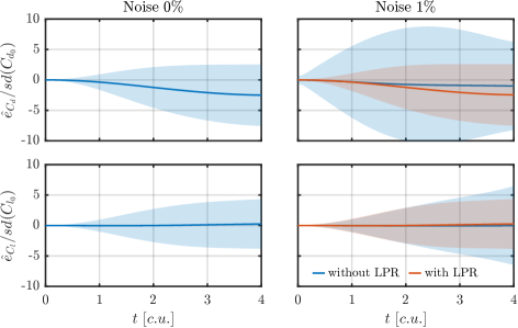
Figure 4: Prediction performance of the force model obtained using SINDYc. The plots display the average value and the confidence region for $\sigma$ of the probability distribution of the normalized $C_{d}$ and $C_{l}$ prediction errors with respect to their standard deviation under unforced conditions. Panels on the left show the results in absence of measurement noise of the initial condition while those on the right with $1\%$ of measurement noise. In the presence of noise, a comparison is shown with the results of predictions obtained using LPR estimation as initial condition.

The panels on the left show the prediction performance calculated from an initial condition obtained in the absence of measurement noise in the sensors. The average value of the normalized error distribution maintains values close to zero for any length of the prediction window analyzed. Furthermore, for short prediction lengths (up to $\approx 3\,c.u.$) the confidence bounds for $\sigma$ are still confined within a narrow region. In this context, as they are not directly measurable, the time derivatives of the aerodynamic coefficients are calculated using finite differences. This approach, however, is highly sensitive to measurement noise. The nonparametric smoothing technique LPR allows joint estimation of the output data from the sensors and their respective time derivatives. The panels on the right show the benefits brought by initial-condition setting with LPR to the prediction performance in the presence of a sensor measurement noise of $1\%$. These plots show a comparison of the statistical error distributions for two distinct cases: in one the initial condition corresponds to the LPR estimation of the data with noise, in the other, it is not used. It is of considerable interest to observe that The prediction with LPR performs similarly to the case without noise. The figure above discussed could be used to choose the MPC prediction window length as it provides an idea of the uncertainty propagation in the prediction horizon. However, since this parameter has a significant effect on control results in terms of performance and computational cost, it is left to automatic selection through Bayesian optimization, so as to also take into account the effects of measurement noise in its selection.

In addition, figure 5 provides further insights into the advantages of LPR. In this case the estimation of $C_{d}$ and $\dot{C_{d}}$ is tested on a case with external forcing and under increasing noise level. The trend in the LPR estimation error of both $C_{d}$ and $\dot{C_{d}}$ is illustrated as the noise increases. The estimation errors are evaluated using a root mean square error (RMSE) of the estimate compared to the ideal data without noise.

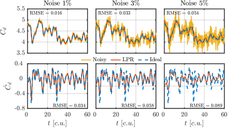
Figure 5: LPR applied to a $C_{d}$ time series within a time period of $60c.u.$. This case corresponds to forced fluidic pinball dynamics. Top panels display $C_{d}$ estimation in the presence of increasing noise levels ($1\%,3\%,5\%$). Bottom panels show LPR estimation of $\dot{C_{d}}$. Each plot includes the ideal and noisy time series, also including the RMSE of the LPR estimation.

The results demonstrate the effectiveness of LPR in estimating $C_{d}$ and $\dot{C_{d}}$ with high accuracy even in the presence of high levels of noise. Thus, the benefits brought by LPR enable the control feasibility even in high-noise scenarios.

3.2 Bayesian optimization for tuning control parameters

This subsection presents the results of the hyperparameters tuning using the Bayesian optimization algorithm. Various control scenarios are analyzed, including clean, low, and high noise level cases.

The set of hyperparameters to be optimized is composed of the elements of the weight matrices in (3) and the length of the control/prediction window, used in the definition of the cost functional in (2). Specifically, the components of the matrix $\mathsfbi{Q}$ are optimized within the interval $[0.1,5]$, the terms of $\mathsfbi{R}_{b}$ and $\mathsfbi{R}_{\Delta b}$ in $[0.1,10]$, and $w_{p}$ is optimized within $[1,4]$.

Figure 6 displays the trend of the minimum observed $\mathcal{J}_{BO}$ samplings as the tuning process iterations progress for some of the analyzed control cases. The results indicate that the optimization function ($\mathcal{J}_{BO}$) reaches convergence in less than 30 iterations for almost all cases.

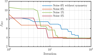
Figure 6: Minimum observed $J_{BO}$ sampling history during MPC hyperparameter tuning. The x-axis of the plot is in logarithmic scale. The results of some control scenarios in presence and absence of measurement noise (and symmetry in the parameters) are presented.

The tuned control parameters of each case are presented in table 1. The table also provides the average values of $C_{d}$ and $C_{l}$ ($\bar{C_{d}}$ and $\bar{C_{l}}$), as well as their corresponding standard deviations ($sd(C_{d})$ and $sd(C_{l})$), during the control phase. These values are computed over a shedding time interval.

It must be remarked that the final set of hyperparameters for each case is run-dependent. This is mostly to be ascribed to the weak dependence of $\mathcal{J}_{BO}$ to some of the imposed constraints in the MPC loss function. Nonetheless, the differences in terms of drag reduction have been observed to be smaller than $\pm 1.1\%$ in different runs.

Figure 7 presents a plot of the cost function $\mathcal{J}_{BO}$ and its contributions due to the control of $C_{d}$ (denoted as $\mathcal{J}_{BO}^{1}$) and $C_{l}$ (denoted as $\mathcal{J}_{BO}^{2}$), varying $Q^{1}$ and $Q^{2}$, and then $R_{b^{1}}$ and $R_{b^{2}}=R_{b^{3}}=R_{b^{2,3}}$ under $1\%$ measurement noise. The two contributions of $\mathcal{J}_{BO}$ can be obtained by considering the cost functional in equation (10) and selecting only the component for $k=1$ (to obtain $\mathcal{J}_{BO}^{1}$) and for $k=2$ to obtain $\mathcal{J}_{BO}^{2}$. The presented cost function plot is useful for interpreting the convergence parameters of the optimization process according to BO. The term $\mathcal{J}_{BO}^{2}$ has a minor influence on the optimization process, being approximately two orders of magnitude smaller than $\mathcal{J}_{BO}^{1}$. Therefore, the optimization process is mainly driven by the influence of the control parameters on reducing the $C_{d}$ of the fluidic pinball.

As $Q^{1}$ increases, both $\mathcal{J}_{BO}$ and $\mathcal{J}_{BO}^{1}$ functions decrease sharply at first and then reach a plateau. Conversely, $\mathcal{J}_{BO}^{2}$ shows the opposite behavior. A good $C_{l}$ control would be achieved with a low $Q^{1}$ and high $Q^{2}$, but this would lead to a poor drag reduction. On the other hand, the choice of $Q^{2}$ has little impact on control performance, as the cost function $\mathcal{J}_{BO}$ remains nearly constant with its variation.

By observing table 1 and considering the behavior of the cost function, it is justified why almost all proposed control cases have $Q^{1}$ very close to the maximum achievable value, while there is greater variability in the selection of $Q^{2}$.

Similarly, due to the fact that the drag reduction drives the optimization process, the parameter that has the greatest influence on $\mathcal{J}_{BO}$ is $R_{b^{2,3}}$. A lower value of $R_{b^{2,3}}$ would assign less weight to the actuation cost of the rear cylinders of the fluidic pinball, allowing for greater rotation intensity. As it will be explained in § 3.3.1, the main contributors to drag reduction are indeed the rear cylinders. On the other hand, the parameter $R_{b^{1}}$ has little impact on the overall control performance since the front cylinder is responsible for the stabilization of the lift coefficient. These latter considerations justify that the optimum $R_{b^{2,3}}$ is achieved at low values, close to the lower possible limit, while greater variability is observed in the optimization of the $R_{b^{1}}$ parameter.

Noise LPR $diag(\mathsfbi{Q}$) diag($\mathsfbi{R}_{b}$) diag($\mathsfbi{R}_{\Delta b}$) $w_{p}$ $(c.u.)$ $\bar{C_{d}}$ $sd(C_{d})$ $\bar{C_{l}}$ $sd(C_{l})$ 0% no (1.000, 1.000) (1.000, 1.000, 1.000) (1.000, 1.000, 1.000) 3.0 3.0598 0.0956 -0.0530 0.1335 $0\%$ no (4.703, 0.206) (6.334, 3.735, 1.147)^∗ (1.754, 0.176, 0.768)^∗ 3.4 1.9685 0.0099 -0.2278 0.0687 $0\%$ no (4.881, 0.435) (5.133, 0.903, 0.903) (8.409, 0.193, 0.193) 3.2 1.9633 0.0094 0.0022 0.0604 $0.5\%$ no (4.886, 0.191) (7.435, 0.514, 0.514) (3.961, 0.465, 0.465) 3.8 1.9373 0.0200 0.0042 0.0863 $0.5\%$ yes (3.836, 2.283) (9.776, 0.337, 0.337) (0.367, 1.465, 1.465) 3.9 1.9294 0.0099 0.0172 0.0909 $1\%$ yes (4.938, 1.753) (5.960, 0.170, 0.170) (1.123, 2.521, 2.521) 4.0 1.9284 0.0091 0.0103 0.0914 $5\%$ yes (4.659, 1.007) (9.556, 0.547, 0.547) (0.135, 1.044, 1.044) 3.0 1.9371 0.0100 0.0110 0.0970

Table 1: Results of the control tuning through Bayesian optimization. A comparison is provided for all the analyzed simulation cases, with a particular focus on the tuning effects due to the intensity of the sensor measurement noise, the use of the LPR technique in the sensor outputs, and the imposition of symmetry in the control parameters. The asterisk (^∗) denotes control cases in which the tuning is performed on all control parameters, without imposing the symmetry condition on the parameters of the rear cylinders of the fluidic pinball. The table also provides the case with all parameters equal to $1$ (except for the prediction/control window set at $3c.u.$)

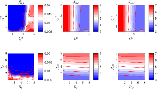
Figure 7: Representation of the cost functional $J_{BO}$ in equation (10), the component due to $C_{l}$ control ($J_{BO}^{2}$), and the component due to $C_{d}$ control ($J_{BO}^{1}$). Contour plots are presented as functions of $Q^{1}$ and $Q^{2}$ (top graphs) and $R_{b^{1}}$ and $R_{b^{2}}=R_{b^{3}}=R_{b^{2,3}}$ (bottom graphs). The control case considers a $1\%$ measurement noise and symmetric weighting coefficients for the rear cylinders of the fluidic pinball. In the graphs, the remaining components of the hyperparameter vector $\boldsymbol{\eta}$ are fixed at their optimal values.

3.3 Application of the MPC-based control algorithm

This subsection shows the results of applying the control algorithm to the wake of the fluidic pinball. It is specified that all results reported from now on are obtained by imposing symmetry in the parameters of the rear cylinders.

3.3.1 Control simulations without measurement noise

Before discussing the effects of MPC-based control, a brief description of the behavior of the unforced wake of the fluidic pinball in the laminar chaotic regime, characteristic of the chosen Reynolds number ($\Rey_{D}=150$), is presented.

Time histories of lift (plot a) and drag (plot b) coefficients for $500\,c.u.$ are reported in figure 8. The figure also includes a power spectral density (PSD) of the lift coefficient (plot c), with the Strouhal number $\mathit{St}_{D}=\frac{fD}{U_{\infty}}$ related to the diameter of the three cylinders, and a representation of the trajectory in the time-delayed embedding space of the force coefficients (plot d). In the chaotic regime of the fluidic pinball, the main peak in the power spectral density of $C_{l}$ is notably broad. However, a predominant one is found corresponding to $\mathit{St}_{D}=0.148$, associated with vortex shedding (with a shedding period $T_{sh}=6.76\,c.u.$). The curve also shows a second peak associated with a lower Strouhal number ($\mathit{St}_{D}=0.013$) due to resonance in the flow field related to the finite size of the domain, as also observed in Deng et al. (2020).

The condition of flow symmetry ($\bar{C_{l}}\approx 0$) is recovered in the chaotic regime, unlike the lower Reynolds number regimes which exhibit non-symmetric wakes (Deng et al., 2020). In addition, $C_{l}$ standard deviation is $sd(C_{l})=0.112$. As for the $C_{d}$, its free dynamics exhibits $\bar{C_{d}}=3.46$ and $sd(C_{d})=0.0658$.

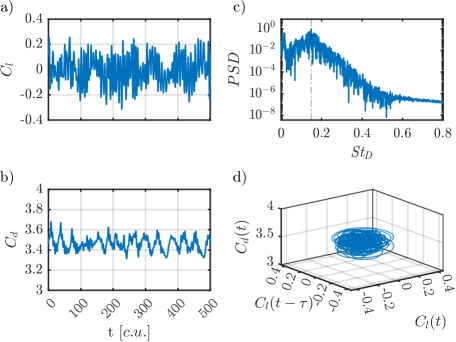
Figure 8: Characteristics of the flow field around the fluidic pinball in undisturbed conditions. Panels a-b) show the global lift and drag coefficients of the fluidic pinball. Plot c) shows a PSD of the lift coefficient while d) provides a representation of the trajectory in the time-delayed embedding space of the force coefficients $C_{d}(t)$, $C_{l}(t)$ and $C_{l}(t-\tau)$, being $\tau$ a quarter of the shedding period of the fluidic pinball wake. The peak in the PSD is at a Strouhal number $\mathit{St}_{D}=0.148$.

Figure 9 shows the controlled case in ideal measurement conditions (i.e. no noise), with the control parameters automatically selected using the Bayesian optimization algorithm. The simulations presented from now on include an initial unforced phase before activating the control at time instant $T_{c}=50\,c.u.$. The plots on the left show the time histories of the controlled aerodynamic coefficients and the exogenous input provided to the system according to the MPC-based control algorithm. Plots $A$, $B$, and $C$, instead, display the streamwise velocity component $u$ averaged over time windows of one shedding period of the fluidic pinball, in correspondence of the unforced, transient, and steady control phases, respectively.

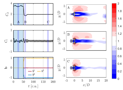
Figure 9: Results of the control application in absence of measurement noise in the sensors. Graphics on the left show the time histories of the $C_{d}$, $C_{l}$ and input vector $\boldsymbol{b}$ during an initial unforced phase and then during an active control phase. Graphics on the right show the mean value of the streamwise component of the velocity ($u$) in the time frames denoted A, B and C, respectively. Black arrows indicate the direction of rotation of the cylinders.

The control automatically selects an implementation law with the two rear cylinders in counter-rotation. The upper cylinder rotates clockwise ($b^{2}=-b^{3}<0$) with nearly constant rotational speed equal to the maximum values set in the optimization problem. This actuation mechanism corresponds to boat tailing, which has been previously observed and studied in various works on control of the wake of fluidic pinball (Raibaudo et al., 2020; Li et al., 2022).

This mechanism primarily aims to reduce the pressure drag of the fluidic pinball. Under unactuated conditions, as observed in plot $A$ of figure 9, an extended recirculation region with low pressure and velocity forms behind the rear cylinders. The boat tailing redirects the shear layers of the top and bottom cylinder toward the pinball axis. This streamlining process of the wake increases the pressure behind the cylinders, delays the separation, and energizes the wake. Furthermore, the gap jet between the cylinders is substantially weakened. A detailed description of this mechanism can be found in Geropp & Odenthal (2000). A full wake stabilization is not achieved, i.e. the vortex shedding is not suppressed, due to the imposed constraints of $\left|{b^{i}}\right|\leq 1$. This is in line with the study of Cornejo Maceda et al. (2021), where wake stabilization in boat tailing is achieved with rotation of the rear cylinder of 2.375 or larger.

A condition of global optimum in terms of minimizing the coefficient of drag would be achieved with an actuation that involves the rear cylinders in boat tailing and the front cylinder in a constant nonzero rotation, as observed in simulations (Li et al., 2022) and also experiments (Raibaudo et al., 2020). The rotation of the front cylinder helps to reduce the low-velocity areas in the region behind the cylinders of the fluidic pinball, allowing for a slight reduction in drag. However, this condition is not achieved in the present case since the control target includes a condition of null $C_{l}$, with the consequence that any asymmetric flow actuation is penalized in the optimization process. MPC, on the other hand, focuses its strategy towards reducing $C_{l}$ oscillations. Cornejo Maceda et al. (2021) document oscillating lift coefficient with amplitude increasing with increasing $b_{2},-b_{3}$ in the range $0-2$ if solely the rear cylinders are put in rotation. The self-tuned MPC converges to an actuation strategy to reduce $C_{l}$ oscillations based on phasor control with the front cylinder.

An examination of the behavior of the drag coefficient ($C_{d}$) resulting from the implementation of the MPC control shows a decrease in its mean value, reducing it by $43.3\%$ compared to the unforced case. Moreover, the standard deviation of the drag coefficient is reduced as well, by $85.8\%$ during forced conditions compared to the unforced ones.

Figure 10 shows the out-of-plane vorticity in three different phases: before, during, and after the application of the control to the fluidic pinball wake. The MPC actuation is able to reduce the interaction between the upper and lower shear layers. In addition, the wake behind the fluidic pinball exhibits a more regular pattern in the post-transient phase. The wake meandering is strongly reduced, possibly due to the front stagnation point control with the front cylinder. The wake streamlining due to the boat tailing effect might also be contributing in this direction. This is also observed in the oscillating behavior of the $C_{l}$, which becomes more regular and with less intense peaks once the control is activated. Indeed, in the controlled phase, the power spectral density of the $C_{l}$ presents a single very narrow peak concentrated at a Strouhal number of $\mathit{St}_{D}\approx 0.14$, resulting in a shedding period of $7.16\,c.u.$, very similar to the predominant shedding frequency in the free response.

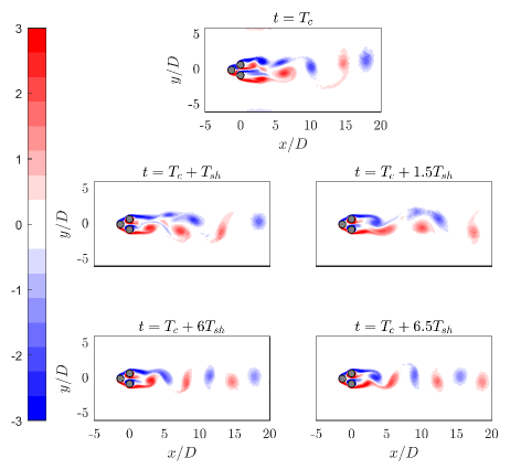
Figure 10: Contour plot of the out-of-plane vorticity component of the flow around the fluidic pinball. Several instants corresponding to the phases of control onset, transient, and post-transient phase are presented. $T_{sh}$ refers to the characteristic shedding period of the fluidic pinball in unforced conditions.

An analysis of the total power trend is required to assess if the MPC is able to achieve a net energy saving. The total power ($P_{tot}$) is characterized by the sum of two contributions: the first is directly related to the drag of the fluidic pinball ($P_{d}$); the second one is associated with the power required for actuation ($P_{a}$). Thus, the total power can be defined as follows:

$$P_{tot}=P_{d}+P_{a}=F_{d}U_{\infty}+\sum_{i=1}^{3}\frac{\tau^{i}b^{i}}{R}$$

being $\tau^{i}$ the torque acting on the $i^{th}$ cylinder of the fluidic pinball. The time history of power during the free and forced phases is given in figure 11. It can be observed that under undisturbed conditions, the total power remains around an average value of $1.75$, with oscillations related only to the drag of the fluidic pinball. When moving to the controlled solution, the total power undergoes a sharp decrease in the transient phase thanks to the boat tailing. The total power stabilizes at about $1.12$, experiencing a reduction of $36.31\%$ compared to the unforced phase. It is also observed that the average actuation power corresponds only to $12.13\%$ of the total power in the controlled phase. The average value of the actuation power is mainly related to the rear cylinders in boat tailing, while its oscillations are due to the front cylinder aiming to control the shedding, in order to reduce the lift fluctuations. It must be remarked though that this does not take into account possible inefficiencies that would arise in an implementation in a real environment.

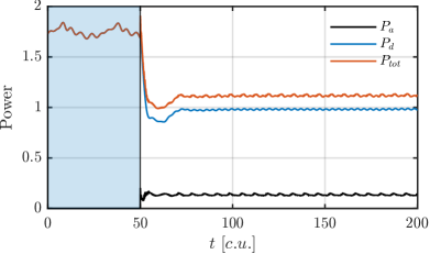
Figure 11: Time histories of the power associated with drag, actuation, and total power during the free and forced stages. Simulation of the fluidic pinball wake control in the absence of measurement noise.

A comparison between the proper orthogonal decomposition (POD) of the flow fields with and without control according to the MPC-based control algorithm is also shown in figure 12. It is specified that the POD has been performed on a dataset including both the transient and the stationary part of the control. On the left side of the figure, the spatial distributions of the 1, 3, and 5 out-of-plane vorticity modes are shown for both free and controlled cases. The plots on the right side of the figure show the eigenvalues of the first $100$ temporal modes. The eigenvalues are normalized with respect to their sum for the case without actuation. This allows a direct comparison of the mode energy in unforced and forced cases.

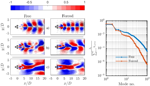
Figure 12: Results of a POD applied to the flow field of the wake past fluidic pinball. Panels on the left, from top to bottom depict the representation of out-of-plane vorticity for the spatial modes $1$, $3$ and $5$ under both free and forced conditions in accordance with the MPC-based control architecture. Every plot also presents velocity vectors corresponding to each spatial mode. The graph on the right shows the squared singular values ($\lambda_{i}$) of the POD, normalized with respect to the sum of the squared singular values for the free case ($\lambda_{i,free}$). POD performed on a dataset consisting of $l=1200$ snapshots of the fluidic pinball wake, including the transient in the forced case.

By observing the graphs related to the POD of the wake dataset under controlled conditions, it is noted that shedding inception is shifted upstream if compared to the unforced condition and is also more regular in the presence of boat tailing of the rear cylinders. Furthermore, the modes of the controlled case, compared to the free case, are characterized by lower energy, with the exception of the first 2 modes. This is ascribed to a partial wake stabilization, with reduced meandering. Mode $1$ spotlights indeed more defined vortical structures, with crosswise width practically constant throughout the wake development. The fluidic boat tailing of the wake has indeed the effect of re-energizing the outer shear layers, redirecting them towards the pinball axis. The wake dynamics shift towards a less chaotic behavior, as also observed in the more regular oscillations of the $C_{l}$ after activation of the control (figure 9). A less rich dynamics results in a more compact POD eigenspectrum for the controlled case, with higher energy in the first two modes. The reduced crosswise oscillations are observed also in the structure of higher-order modes. Modes $3-6$ for the uncontrolled case embed the energy of higher-order harmonics and model the crosswise wake oscillations. In addition to the fluidic boat tailing due the the rotation of the rear cylinders, the stagnation point control enforced by the front cylinder has the effect of weakening such oscillations. This results in lower energy for the corresponding POD modes in the controlled case, and a more compact structure of their vortical features.

3.3.2 The effects of measurements noise in the sensors

The self-tuned control strategy with online LPR of the sensor signal is assessed in the presence of noise. The control results in terms of $C_{d}$ and $C_{l}$ and actuation are given in figure 13. We include as a reference the case of MPC without hyperparameter tuning, i.e. the control parameters are manually selected and all set to unity (except for the prediction/control window set to $3c.u.$). The outcomes when the parameter selection is automatically performed using BO is reported for different noise level. Without hyperparameter tuning, the performance of the control is quite poor for both $C_{d}$ and $C_{l}$. In this case, the mean drag coefficient is $3.0598$, i.e. significantly larger than the value of $\approx 1.97$ achieved after hyperparameter tuning. Furthermore, MPC converges to an asymmetric controlled state, with a negative average lift coefficient. Quite surprisingly, this is achieved even if $R_{b^{2}}=R_{b^{3}}=1$, i.e. forcing symmetry in the hyperparameters does not necessarily lead to symmetric actuation. After hyperparameter tuning, the penalty weight of actuation (and actuation variability) on the rear cylinder is decreased with respect to the front cylinder (see Table 1). This allows stronger actuation on the rear cylinders, thus fostering strong fluidic boat tailing, with consequent strong drag reduction, accompanied by a weak action of the front cylinder to improve wake stability.

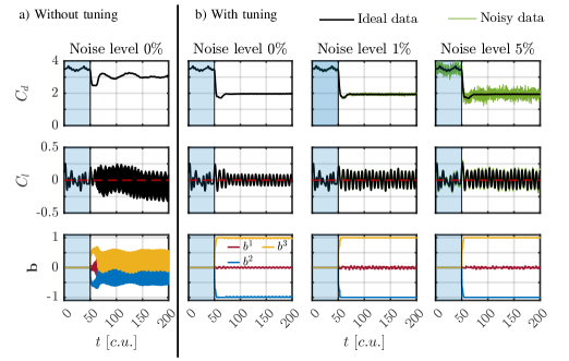
Figure 13: Time series of $C_{d}$, $C_{l}$ and exogenous input $b^{i}$ (from top to bottom row, respectively) at free and forced conditions according to the MPC-based control framework applied to the fluidic Pinball. The panels in a) show the results when the cost function parameters are hand-selected and equal to the unity (with the exception of the prediction control window, set to $3c.u.$). The panels in b) show the results when Bayesian Optimization is used for hyperparameter tuning. LPR is included in the MPC control framework in all cases where measurement noise is present.

The cases analyzed above are reproduced also in figure 14 in terms of trajectories of $C_{d}(t)$, $C_{l}(t)$, and $C_{l}(t-\tau)$ where $\tau$ corresponds to a quarter of the shedding period $T_{sh}$ of the fluidic pinball wake. The plots offer a description of the attractor onto which the wake dynamics of the fluidic pinball evolves, including the transitional phase from free to forced conditions. When the parameter tuning is performed, during the control $C_{d}$ experiences a remarkable reduction, whereas $C_{l}$ evolves on a dynamics similar to the unforced case, although less chaotic. Nevertheless, it is worth noting that the control of $C_{l}$ is not perfectly attained, as the model uncertainties hinder a complete description of the shedding dynamics of the fluidic pinball. Without hyperparameter tuning, in the first part of the transient the system transitions initially towards a state with a lower average $C_{d}$ (around 2.5) and $C_{l}$ oscillations of slightly lower intensity. The relatively high penalty on the actuation of the rear cylinders with respect to the front one, however, forces the system to avoid strong boat tailing and starts leveraging asymmetric actuation based on the front cylinder in the attempt to stabilize the wake through stagnation point control. The system finally converges to a limit cycle with a higher average $C_{d}$ and with large oscillations of the $C_{l}$ around a negative average.

In terms of the $C_{d}$, the control remains nearly unaffected by variations in measurement noise in the sensors. Regardless of the noise intensity, the posterior cylinders consistently maintain their boat tailing configuration, exhibiting maximum rotational velocity limited by the actuation constraints. On the other hand, the control of the lift coefficient demonstrates higher sensitivity to measurement noise. This is attributed to the increased susceptibility of the predictive model to disturbances in the initial conditions of online predictions. As the measurement noise intensifies, the frontal cylinder displays larger oscillations in the selected actuation law prescribed by the MPC-based control.

Nevertheless, LPR provides advantages to the algorithm, resulting in only marginal degradation of control performance. This increases the robustness of the application in realistic control scenarios characterized by high sensor noise.

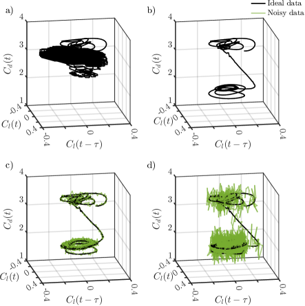
Figure 14: Trajectories in the time-delayed embedding space of the force coefficients $C_{d}(t)$, $C_{l}(t)$ and $C_{l}(t-\tau)$, being $\tau$ a quarter of the shedding period of the fluidic pinball wake. The panel in a) shows the results when the cost function parameters are hand-selected and equal to the unity, while panels b-d) show the result when Bayesian Optimization is used for hyperparameter tuning. Cases a) and b) relate to ideal measurement conditions while cases c) and d) have noise of $1\%$ and $5\%$, respectively. LPR is included in the MPC control framework in all cases where measurement noise is present.

3.3.3 Symmetry in rear cylinder parameters

This part is intended to provide more details about the choice of symmetry in the control parameters. Specifically, it concerns the components of the weight matrices that penalize the input expenditures and input variability of the rear cylinders during control, already introduced in § 2.1.4.

The results of the control simulations with and without imposed symmetry conditions are presented in figure 15. A certain bias is observed in the control of $C_{l}$ in the case without imposing symmetry conditions. This is related to an asymmetry in the rotation of the rear cylinders. However, under imposed symmetry, the control of the drag coefficient improves slightly, as the tangential speeds of rotation of the rear cylinders are both at the actuation limits, creating a stronger boat tailing. This lower effectiveness of the optimization in the case without imposed symmetry can be explained by the relatively low importance of the $C_{l}$ fluctuations in the functional of Bayesian optimization in equation (10), as discussed in § 3.2. The implementation of a law that binds the parameters of the rear cylinders reduces the total number of parameters to be tuned, leading to a less computationally expensive offline phase of the control.

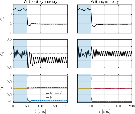
Figure 15: Results of the application of MPC-based control in terms of $C_{d}$, $C_{l}$, and input vector $\boldsymbol{b}$, without (left panels) and with (right panels) the imposition of symmetry in the parameters related to the rear cylinders. In both cases, all the parameters are tuned using BO algorithm. Results of control in the absence of measurement noise in the sensors.

4 Discussion and conclusion

In this work, a noise-robust MPC-based control algorithm that does not require user intervention neither for the plant modeling nor for the hyperparameters selection is proposed. The model used in the MPC optimization is selected from input-output data of the system under control using nonlinear system identification. The control parameters are automatically selected using a black-box optimization based on Bayesian methods. Additionally, the robustness of the algorithm is enhanced by the nonparametric smoothing technique LPR, which acts on the output data from the control sensors to address the presence of measurement noise.

The proposed control algorithm is successfully applied to the control of the wake of the fluidic pinball for drag reduction in a chaotic regime (specifically, for $\Rey_{D}=150$) using solely aerodynamic forces to guide the control strategy. The methodology achieves good success in controlling a non-linear, chaotic, and high-dimensional system. Being based on the MPC technique, the algorithm easily allows for the inclusion of non-linear constraints in the control and is very promising for applications where the control target is not a simple setpoint stabilization.

The proposed technique has shown to be highly robust to sensor measurement uncertainty, performing excellently even in realistic control scenarios characterized by a high level of noise. It must be remarked that, although rather realistic for force measurements, the Gaussian noise model might not be adequate if other sensing techniques are used. This may have an impact on plant model identification and LPR performance. However, the most attractive feature is that the method requires minimal user interaction, as the control parameters are automatically tuned by the Bayesian optimization algorithm according to the control target, taking into account also different fidelity levels for the plant predictions. The automatic procedure identified the most rewarding directions to optimize parameters with the aid only of a few numerical experiments. To control $C_{d}$ and $C_{l}$ of the fluidic pinball around a zero setpoint the MPC algorithm used a combination of two control mechanisms that have been previously considered in fluidic pinball control works: the boat tailing of the rear cylinders for drag reduction and the stagnation point control of the front cylinder for shedding control. This corresponded to a stronger penalty on the $C_{d}$ and a low penalty on the actuation cost of the rear cylinders. Without the framework proposed in this work, this process would have required parametric studies or sub-optimal analysis, with the inherent difficulty of choosing relative weights between heterogeneous quantities.

It is worth highlighting that the control algorithm is currently being tested on a control case with relatively simple dynamics (Deng et al., 2020, 2022). This streamlines the process of coordinate selection and nonlinear system identification using the SINDYc technique. On the one hand, the aerodynamic force coefficients in separated wake flows exhibit features that render them suitable for plant modeling. On the other hand, the dynamics of the flow, although chaotic, evolve clearly on a low-dimensional attractor, thus simplifying the library selection for the application of SINDYc. For more complex flows (higher Reynolds number or with less clear features for straightforward coordinate identification) we envision that the challenge of MPC application will reside mostly in the coordinate selection and in the plant identification. Fast-paced advancements in grey- and black-box modeling are paving the way to interesting research pathways in these directions. The approach proposed here, however, will still be applicable and will benefit from such advancements. The offline optimization of the hyperparameters of the cost function can be applied independently of the method for coordinate selection or plant identification. Furthermore, the outcome will automatically adapt to the fidelity of the model plant when compared to the uncertainty of the measurements used to feed it. [Funding]The authors acknowledge the support from the research project PREDATOR-CM-UC3M. This project has been funded by the call ”Estímulo a la Investigación de Jóvenes Doctores/as” within the frame of the Convenio Plurianual CM-UC3M and the V PRICIT (V Regional Plan for Scientific Research and Technological Innovation).

[Acknowledgements]The authors thank Prof. B. Noack, from Harbin Institute of Technology, and Prof. M. Morzynski, from Poznan University of Technology, for providing the code for the fluidic pinball simulations, and Dr. G. Cornejo Maceda for the post-processing code for force estimation. The authors also thank three anonymous referees for numerous useful comments that significantly improved this article.

[Declaration of interests]The authors report no conflict of interest.

[Data availability statement]The code used in this work is made available at: https://github.com/Lmarra1/Self-tuning-model-predictive-control-for-wake-flows. The dataset is openly available in Zenodo, accessible through the following link: https://doi.org/10.5281/zenodo.10530019

[Author ORCIDs]
L. Marra, https://orcid.org/0000-0001-9422-2808;
A. Meilán-Vila, https://orcid.org/0000-0001-8537-9280;
S. Discetti, https://orcid.org/0000-0001-9025-1505

References

- Ahuja et al. (2007) Ahuja, S., Rowley, C., Kevrekidis, I., Wei, M., Colonius, T. & Tadmor, G. 2007 Low-dimensional models for control of leading-edge vortices: equilibria and linearized models. In 45th AIAA Aerospace Sciences Meeting and Exhibit, p. 709.
- Allgöwer et al. (2004) Allgöwer, F., Findeisen, R., Nagy, Z. K. & others 2004 Nonlinear model predictive control: From theory to application. J. Chin. Inst. Chem. Eng. 35 (3), 299–316.
- Beintema et al. (2020) Beintema, G., Corbetta, A., Biferale, L. & Toschi, F. 2020 Controlling rayleigh–bénard convection via reinforcement learning. J. Turbul. 21 (9-10), 585–605, arXiv: https://doi.org/10.1080/14685248.2020.1797059.
- Bewley et al. (2001) Bewley, T. R., Moin, P. & Temam, R. 2001 Dns-based predictive control of turbulence: an optimal benchmark for feedback algorithms. J. Fluid Mech. 447, 179–225.
- Bieker et al. (2020) Bieker, K., Peitz, S., Brunton, S. L., Kutz, J. N. & Dellnitz, M. 2020 Deep model predictive control with online learning for complex physical systems. Theoretical and Computational Fluid Dynamics 34 (10).
- Blackburn & Henderson (1999) Blackburn, H. M. & Henderson, R. D. 1999 A study of two-dimensional flow past an oscillating cylinder. J. Fluid Mech. 385, 255–286.
- Bøhn et al. (2023) Bøhn, E., Gros, S., Moe, S. & Johansen, T. A. 2023 Optimization of the model predictive control meta-parameters through reinforcement learning. Eng. Appl. Artif. Intell. 123, 106211.
- Brunton & Noack (2015) Brunton, S. L. & Noack, B. R. 2015 Closed-loop turbulence control: Progress and challenges. Appl. Mech. Rev. 67 (5).
- Brunton et al. (2016a) Brunton, S. L., Proctor, J. L. & Kutz, J. N. 2016a Discovering governing equations from data by sparse identification of nonlinear dynamical systems. Proc. Natl. Acad. Sci. U.S.A. 113 (15), 3932–3937.
- Brunton et al. (2016b) Brunton, S. L., Proctor, J. L. & Kutz, J. N. 2016b Sparse identification of nonlinear dynamics with control (sindyc). IFAC-PapersOnLine 49 (18), 710–715, 10th IFAC Symposium on Nonlinear Control Systems NOLCOS 2016.
- Buche et al. (2002) Buche, D., Stoll, P., Dornberger, R. & Koumoutsakos, P. 2002 Multiobjective evolutionary algorithm for the optimization of noisy combustion processes. IEEE Trans. Syst. Man Cybern. 32 (4), 460–473.
- Camacho & Alba (2013) Camacho, E. F. & Alba, C. B. 2013 Model predictive control. Springer science & business media.
- Castellanos et al. (2022a) Castellanos, R., Cornejo Maceda, G. Y., de la Fuente, I., Noack, B. R., Ianiro, A. & Discetti, S. 2022a Machine-learning flow control with few sensor feedback and measurement noise. Phys. Fluids 34 (4), 047118.
- Castellanos et al. (2022b) Castellanos, R., Michelis, T., Discetti, S., Ianiro, A. & Kotsonis, M. 2022b Reducing turbulent convective heat transfer with streamwise plasma vortex generators. Exp. Therm. Fluid Sci. 134, 110596.
- Cetiner & Rockwell (2001) Cetiner, O. & Rockwell, D. 2001 Streamwise oscillations of a cylinder in a steady current. part 1. locked-on states of vortex formation and loading. J. Fluid Mech. 427, 1–28.
- Chevalier et al. (2007) Chevalier, M., Hœpffner, J., Åkervik, E. & Henningson, D. S. 2007 Linear feedback control and estimation applied to instabilities in spatially developing boundary layers. J. Fluid Mech. 588, 163–187.
- Collis et al. (2000) Collis, S., Chang, Y., Kellogg, S. & Prabhu, R. 2000 Large eddy simulation and turbulence control. In Fluids 2000 Conference and Exhibit, p. 2564.
- Cornejo Maceda et al. (2021) Cornejo Maceda, G. Y., Li, Y., Lusseyran, F., Morzyński, M. & Noack, B. R. 2021 Stabilization of the fluidic pinball with gradient-enriched machine learning control. J. Fluid Mech. 917, A42.
- Corona & De Schutter (2008) Corona, D. & De Schutter, B. 2008 Adaptive cruise control for a smart car: A comparison benchmark for mpc-pwa control methods. IEEE Trans. Control Syst. Technol. 16 (2), 365–372.
- Cortelezzi & Speyer (1998) Cortelezzi, L. & Speyer, J. L. 1998 Robust reduced-order controller of laminar boundary layer transitions. Phys. Rev. E. 58 (2), 1906.
- Deng et al. (2020) Deng, N., Noack, B. R., Morzyński, M. & Pastur, L. R. 2020 Low-order model for successive bifurcations of the fluidic pinball. J. Fluid Mech. 884, A37.
- Deng et al. (2022) Deng, N., Noack, B. R., Morzyński, M. & Pastur, L. R. 2022 Cluster-based hierarchical network model of the fluidic pinball–cartographing transient and post-transient, multi-frequency, multi-attractor behaviour. J. Fluid Mech. 934, A24.
- Duriez et al. (2017) Duriez, T., Brunton, S. L. & Noack, B. R. 2017 Machine learning control-taming nonlinear dynamics and turbulence, , vol. 116. Springer.
- Edwards et al. (2021) Edwards, W., Tang, G., Mamakoukas, G., Murphey, T. & Hauser, K. 2021 Automatic tuning for data-driven model predictive control. In 2021 IEEE International Conference on Robotics and Automation (ICRA), pp. 7379–7385. IEEE.
- Fan et al. (2020) Fan, D., Yang, L., Wang, Z., Triantafyllou, M. S. & Karniadakis, G. E. 2020 Reinforcement learning for bluff body active flow control in experiments and simulations. Proc. Natl. Acad. Sci. U.S.A. 117 (42), 26091–26098.
- Fan & Gijbels (1996) Fan, J. & Gijbels, I. 1996 Local polynomial modelling and its applications. Monographs on statistics and applied probability series 66. London [u.a.]: Chapman & Hall.
- Fröhlich et al. (2022) Fröhlich, L. P., Küttel, C., Arcari, E., Hewing, L., Zeilinger, M. N. & Carron, A. 2022 Contextual tuning of model predictive control for autonomous racing. In 2022 IEEE/RSJ International Conference on Intelligent Robots and Systems (IROS), pp. 10555–10562. IEEE.
- Gautier et al. (2015) Gautier, N., Aider, J.-L., Duriez, T., Noack, B. R., Segond, M. & Abel, M. 2015 Closed-loop separation control using machine-learning. J. Fluid Mech. 770, 442–457.
- Gerhard et al. (2003) Gerhard, J., Pastoor, M., K., R., Noack, B., Dillmann, A., Morzynski, M. & Tadmor, G. 2003 Model-based control of vortex shedding using low-dimensional galerkin models. In 33rd AIAA fluid dynamics conference and exhibit, p. 4262.
- Geropp & Odenthal (2000) Geropp, D. & Odenthal, H.-J. 2000 Drag reduction of motor vehicles by active flow control using the coanda effect. Exp. Fluids 28 (1), 74–85.
- Giordano & Parrella (2008) Giordano, F. & Parrella, M. L. 2008 Neural networks for bandwidth selection in local linear regression of time series. Comput. Stat. Data Anal. 52 (5), 2435–2450.
- Green (2003) Green, J. E. 2003 Civil aviation and the environmental challenge. Aeronaut. J. 107 (1072), 281–299.
- Grüne & Pannek (2017) Grüne, L. & Pannek, J. 2017 Nonlinear model predictive control. In Nonlinear model predictive control. Springer Cham.
- Gad-el Hak (2000) Gad-el Hak, M. 2000 Flow Control: Passive, Active, and Reactive Flow Management. Cambridge University Press.
- Henson (1998) Henson, M. A. 1998 Nonlinear model predictive control: current status and future directions. Comput. Chem. Eng. 23 (2), 187–202.
- Hewing et al. (2020) Hewing, L., Wabersich, K. P., Menner, M. & Zeilinger, M. N. 2020 Learning-based model predictive control: Toward safe learning in control. Annu. Rev. Control Robot. Auton. Syst. 3 (1), 269–296.
- Illingworth et al. (2011) Illingworth, S. J., Morgans, A. S. & Rowley, C. W. 2011 Feedback control of flow resonances using balanced reduced-order models. J. Sound Vib. 330 (8), 1567–1581.
- Kaiser et al. (2018) Kaiser, E., Kutz, J. N. & Brunton, S. L. 2018 Sparse identification of nonlinear dynamics for model predictive control in the low-data limit. Proc. R. Soc. Lond. 474 (2219), 20180335.
- Kaiser et al. (2017) Kaiser, E., Noack, B. R., Spohn, A., Cattafesta, L. N. & Morzyński, M. 2017 Cluster-based control of a separating flow over a smoothly contoured ramp. Theor. Comput. Fluid Dyn. 31, 579–593.
- Kim (2011) Kim, J. 2011 Physics and control of wall turbulence for drag reduction. Philos. Trans. Royal Soc. A 369 (1940), 1396–1411.
- Kim & Bewley (2007) Kim, J. & Bewley, T. R. 2007 A linear systems approach to flow control. Annu. Rev. Fluid Mech. 39 (1), 383–417.
- Koumoutsakos et al. (2001) Koumoutsakos, P., Freund, J. & Parekh, D. 2001 Evolution strategies for automatic optimization of jet mixing. AIAA J. 39 (5), 967–969, arXiv: https://doi.org/10.2514/2.1404.
- Lee (2011) Lee, J. H. 2011 Model predictive control: Review of the three decades of development. Int. J. Control. Autom. 9 (3), 415–424.
- Lee et al. (2001) Lee, K. H., Cortelezzi, L., Kim, J. & Speyer, J. 2001 Application of reduced-order controller to turbulent flows for drag reduction. Phys. Fluids 13 (5), 1321–1330.
- Li et al. (2022) Li, Y., Cui, W., Jia, Q., Li, Q., Yang, Z., Morzyński, M. & Noack, B. R. 2022 Explorative gradient method for active drag reduction of the fluidic pinball and slanted ahmed body. J. Fluid Mech. 932, A7.
- Little et al. (2007) Little, J., Debiasi, M., Caraballo, E. & Samimy, M. 2007 Effects of open-loop and closed-loop control on subsonic cavity flows. Phys. Fluids 19 (6).
- Loiseau et al. (2018) Loiseau, J. C., Noack, B. R. & Brunton, S. L. 2018 Sparse reduced-order modelling: sensor-based dynamics to full-state estimation. J. Fluid Mech. 844, 459–490.
- Monokrousos et al. (2008) Monokrousos, A., Brandt, L., Schlatter, P. & Henningson, D. S. 2008 Dns and les of estimation and control of transition in boundary layers subject to free-stream turbulence. Int. J. Heat Fluid Flow 29 (3), 841–855.
- Morton et al. (2018) Morton, J., Jameson, A., Kochenderfer, M. J. & Witherden, F. 2018 Deep dynamical modeling and control of unsteady fluid flows. In Advances in Neural Information Processing Systems (ed. S. Bengio, H. Wallach, H. Larochelle, K. Grauman, N. Cesa-Bianchi & R. Garnett), , vol. 31. Curran Associates, Inc.
- Nagarajan et al. (2018) Nagarajan, K. K., Singha, S., Cordier, L. & Airiau, C. 2018 Open-loop control of cavity noise using proper orthogonal decomposition reduced-order model. Comput Fluids 160, 1–13.
- Nair et al. (2019) Nair, A. G., Yeh, Chi-An, Kaiser, E., Noack, B. R., Brunton, S. L. & Taira, K. 2019 Cluster-based feedback control of turbulent post-stall separated flows. J. Fluid Mech. 875, 345–375.
- Noack & Morzyński (2017) Noack, B. R. & Morzyński, M. 2017 The fluidic pinball—a toolkit for multiple-input multiple-output flow control (version 1.0). Tech. Rep.. Tech. Rep. 02/2017. Chair of Virtual Engineering, Poznan University of Technology.
- Ouyang et al. (2018) Ouyang, L., Zhou, D., Ma, Y. & Tu, Y. 2018 Ensemble modeling based on 0–1 programming in micro-manufacturing process. Comput. Ind. Eng. 123, 242–253.
- Parkin et al. (2014) Parkin, D. J., Thompson, M. C. & Sheridan, J. 2014 Numerical analysis of bluff body wakes under periodic open-loop control. J. Fluid Mech. 739, 94–123.
- Pastur et al. (2019) Pastur, L. R., Deng, N., Morzyński, M. & Noack, B. R. 2019 Reduced-order modeling of the fluidic pinball. In Chaotic Modeling and Simulation International Conference, pp. 205–213. Springer, Cham: Springer International Publishing.
- Peitz et al. (2020) Peitz, S., Otto, S. E. & Rowley, C. W. 2020 Data-driven model predictive control using interpolated koopman generators. SIAM J. Appl. Dyn. Syst. 19 (3), 2162–2193.
- Pinier et al. (2007) Pinier, J. T., Ausseur, J. M., Glauser, M. N. & Higuchi, H. 2007 Proportional closed-loop feedback control of flow separation. AIAA J. 45 (1), 181–190.
- Poncet et al. (2005) Poncet, P., Cottet, G. H. & Koumoutsakos, P. 2005 Control of three-dimensional wakes using evolution strategies. CR Mécanique 333 (1), 65–77, high-order methods for the numerical simulation of vortical and turbulent flows.
- Qin & Badgwell (2003) Qin, S. J. & Badgwell, T. A. 2003 A survey of industrial model predictive control technology. Control Eng. Pract. 11 (7), 733–764.
- Rabault et al. (2019) Rabault, J., Kuchta, M., Jensen, A., Réglade, U. & Cerardi, N. 2019 Artificial neural networks trained through deep reinforcement learning discover control strategies for active flow control. J. Fluid Mech. 865, 281–302.
- Raibaudo et al. (2020) Raibaudo, C., Zhong, P., Noack, B. R. & Martinuzzi, R. J. 2020 Machine learning strategies applied to the control of a fluidic pinball. Phys. Fluids 32 (1), 015108.
- Raković & Levine (2018) Raković, S. V. & Levine, W. S. 2018 Handbook of Model Predictive Control. Control engineering 1. Cham: Springer International Publishing AG.
- Rowley & Williams (2006) Rowley, C. W. & Williams, D. R. 2006 Dynamics and control of high-reynolds-number flow over open cavities. Annu. Rev. Fluid Mech. 38, 251–276.
- Sasaki & Tsubakino (2020) Sasaki, Y. & Tsubakino, D. 2020 Designs of feedback controllers for fluid flows based on model predictive control and regression analysis. Energies 13 (6), 1325.
- Schumm et al. (1994) Schumm, M., Berger, E. & Monkewitz, P. A. 1994 Self-excited oscillations in the wake of two-dimensional bluff bodies and their control. J. Fluid Mech. 271, 17–53.
- Shimomura et al. (2020) Shimomura, S., Sekimoto, S., Oyama, A., Fujii, K. & Nishida, H. 2020 Closed-loop flow separation control using the deep q network over airfoil. AIAA J. 58 (10), 4260–4270.
- Sipp (2012) Sipp, D. 2012 Open-loop control of cavity oscillations with harmonic forcings. J. Fluid Mech. 708, 439–468.
- Snoek et al. (2012) Snoek, J., Larochelle, H. & Adams, R. 2012 Practical bayesian optimization of machine learning algorithms. In Advances in Neural Information Processing Systems (ed. F. Pereira, C. J. Burges, L. Bottou & K. Q. Weinberger), , vol. 25. Curran Associates, Inc.
- Steffen et al. (2010) Steffen, J., Oztop, E. & Ritter, H. 2010 Structured unsupervised kernel regression for closed-loop motion control. In 2010 IEEE/RSJ International Conference on Intelligent Robots and Systems, pp. 75–80.
- Tadmor et al. (2011) Tadmor, G., Lehmann, O., Noack, B. R., Cordier, L., Delville, J., Bonnet, J. P. & Morzyński, M. 2011 Reduced-order models for closed-loop wake control. Philosophical Transactions of the Royal Society A: Mathematical, Physical and Engineering Sciences 369 (1940), 1513–1524.
- Thiria et al. (2006) Thiria, B., Goujon-Durand, S. & Wesfreid, J. E. 2006 The wake of a cylinder performing rotary oscillations. J. Fluid Mech. 560, 123–147.
- Tol et al. (2019) Tol, H. J., De Visser, C. C. & Kotsonis, M. 2019 Experimental model-based estimation and control of natural tollmien–schlichting waves. AIAA J. 57 (6), 2344–2355.
- Wand & Jones (1994) Wand, M. P. & Jones, M. C. 1994 Kernel Smoothing. Chapman & Hall/CRC Monographs on Statistics & Applied Probability 60. Boca Raton, FL, U.S.: Chapman & Hall.
- Wang et al. (2023) Wang, X., Deng, N., Cornejo Maceda, G. Y. & Noack, B. R. 2023 Cluster-based control for net drag reduction of the fluidic pinball. Phys. Fluids 35 (2).
- Wu et al. (2018) Wu, Z., Fan, D., Zhou, Y., Li, R. & Noack, B. R. 2018 Jet mixing optimization using machine learning control. Exp. Fluids 59, 1–17.