The trivariate wrapped Cauchy copula - a multi-purpose model for angular data

Abstract

In this paper, we will present a new flexible distribution for three-dimensional angular data, or data on the three-dimensional torus. Our trivariate wrapped Cauchy copula has the following benefits: (i) simple form of density, (ii) adjustable degree of dependence between every pair of variables, (iii) interpretable and well-estimable parameters, (iv) well-known conditional distributions, (v) a simple data generating mechanism, (vi) unimodality. Moreover, our construction allows for linear marginals, implying that our copula can also model cylindrical data. Parameter estimation via maximum likelihood is explained, a comparison with the competitors in the existing literature is given, and two real datasets are considered, one concerning protein dihedral angles and another about data obtained by a buoy in the Adriatic Sea.

1 Introduction

Angular data occur frequently in domains such as environmental sciences (e.g., wind directions, wave directions), bioinformatics (dihedral angles in protein backbone structures), zoology (animal movement studies), medicine (circadian body clock, secretion times of hormones), or political/social sciences (times of crimes during the day), to cite but these [43]. Dealing with data that are angles requires special care in order to take into account their topology (domain $[0,2\pi)$ where the end points coincide). Classical statistical concepts from the real line no longer hold for such data [22, 48]; in particular, the building blocks of statistical modeling and inference, probability distributions, need to be properly defined. For data involving a single angle, called circular data, a large body of literature proposing more or less flexible distributions exists (see [50] and [57]), among which the popular von Mises, wrapped Cauchy, cardioid, Jones–Pewsey [28] and Kato–Jones [34] models. Though less in number, there also exist several interesting distributions for data consisting respectively of two angles, called toroidal data, and an angle and a linear part, called cylindrical data. Popular examples for toroidal distributions are the bivariate von Mises [46], the Sine [61] and Cosine models [51] and the bivariate wrapped Cauchy [35], while examples for cylindrical models are the Johnson–Wehrly [26], the Mardia–Sutton [45], the Kato–Shimizu [36] and the Abe–Ley [1] distributions.

The situation is very different when the data consists of either three angles, two angles and one linear component, or one angle and two linear components. The few existing proposals suffer from problems of tractability, complex parameter estimation procedures, lack of practically usable random number generation or non-interpretable parameters (see Section 6 for details). This is all the more unfortunate as various such datasets exist and demand an adequate statistical treatment. Two important examples are the following:

• Predicting the three-dimensional folding structure of a protein from its known one-dimensional amino acid structure is among the most important yet hardest scientific challenges, with impacts in drug development, vaccine design, disease mechanism understanding, human cell injection, and enzyme engineering, to cite but these. The recent Nature Methods paper [40] concretely stated the need to complement the famous AlphaFold single point prediction with an adequate statistical uncertainty treatment: “distributions of conformations are the future of structural biology” (see our Section 7.1 for details). So far most statistical advances, in particular on flexible and tractable probability distributions, have considered the dihedral angles $\phi$ and $\psi$, and considered the torsion angle of the side chain $\omega$ to be fixed at either 0 or $\pi$ (which are the only two realistic values for this angle). However in practice this angle is often measured with some noise, hence a model for $\phi,\psi$ and $\omega$ is required.

• Many environmental agencies are collecting data on wave heights and directions in order to identify sea regimes. Such identification is highly relevant in climate-change times for studies of the drift of floating objects and oil spills, coastal erosion, and the design of off-shore structures, to cite but these. Typically, the state-of-the-art data analysis procedures use cylindrical distributions (e.g., the Abe–Ley distribution in [39]) to jointly model wave height and direction. An even more informative way to proceed consists in adding information on the wind direction as it heavily influences waves. Quoting [39],“In wintertime, relevant events in the Adriatic Sea are typically generated by the southeastern Sirocco wind and the northern Bora wind". This adds a second angle to the cylindrical data on waves.

Describing a random phenomenon with a probability distribution is not a goal per se but rather inscribes itself in a bigger picture of statistical uncertainty quantification. Besides easing data analysis by providing information about aspects such as central tendency, concentration, asymmetry or dependence, it also allows the calculation of relevant quantities such as risk of exceeding a certain threshold, it forms the basis of statistical methods such as regression, time series analysis or clustering (via mixture models), and it paves the way for stochastic modeling in situations where it is too complicated to calculate the probabilities of some events (e.g., in protein folding where simulations are crucial). All these desirable consequences of fitting a probability distribution to data can only be leveraged if the model satisfies a number of conditions, as laid out in [41]: versatility (ability to exhibit distinct shapes), tractability, parameter interpretability, (ideally simple) data generation mechanism, and fast parameter estimation procedure. As we will describe in Section 6, none of the existing models for trivariate toroidal data satisfies these requirements.

In order to fill this important gap in the literature, we propose in this paper the trivariate wrapped Cauchy copula. By their very nature, copula-based approaches are tailor-made for versatility as copulas are distributions (with uniform marginals) which regulate the dependence structure and can be combined with user-chosen marginals to form highly flexible new models. Indeed, from Sklar’s Theorem [62] we know that any multivariate (on $\mathbb{R}^{d}$) cumulative distribution function (cdf) $F$ can be expressed under the form $F(x_{1},\ldots,x_{d})=C(F_{1}(x_{1}),\ldots,F_{d}(x_{d}))$ with $C$ a $d$-dimensional copula and $F_{1},\ldots,F_{d}$ marginal univariate cdfs, and conversely any copula $C$ can be combined with marginals to produce a multivariate distribution. Well-known references on copulas include [23], [55] and [24]. Copula models have successfully been used in numerous domains such as medicine, finance, actuarial sciences, hydrology or environmental sciences, see e.g. [14], [44], [7], among many others. In the case of angular data, copulas need to fulfil the additional condition of $2\pi$-periodicity and its marginals are not uniform on $[0,1]$ but on the unit circle. Our construction will be such that linear marginals are also admissible, in order to also cover cylindrical data. We attract the reader’s attention to the fact that [29] coined the term circulas for copulas on the torus. In this paper we shall consistently use the word copula since our model also covers linear marginals.

Our trivariate wrapped Cauchy copula has the following further benefits: (i) simple form of density, (ii) adjustable degree of dependence, (iii) interpretable and well-estimatable parameters, (iv) well-known conditional distributions, (v) a simple data generating mechanism, and (vi) unimodality. Thus we are proposing a new model that satisfies all the aforementioned requirements on flexible distributions, plus the agreeable form of conditional distributions is tailor-made for regression. Since our model allows for linear marginals, it not only covers toroidal data but also cylindrical data, unlike the toroidal competitor models from the literature. Moreover, it responds to needs from nonparametric approaches on the torus regarding plug-in rules as expressed in [2] (quotation: “Further research needs to be done as numerically computing the quantities replaced by a parametric circula may be (too) computationally exhaustive with the current circulas available in the literature”).

The rest of the paper is organized as follows. In Section 2 we review some well-known and relevant for our construction bivariate distributions before proposing the trivariate wrapped Cauchy copula. In Section 3, several properties of the proposed distribution are given, including conditional distributions, random variate generation, unimodality and moments. Parameter estimation is considered in Section 4 and the use of non-uniform marginal distributions in Section 5. A thorough comparison with the competitors in the existing literature is given in Section 6 and in Section 7 two real datasets are investigated by means of our new proposal, the first about protein dihedral angles and the second about data obtained by a buoy in the Adriatic Sea. Conclusions and final comments can be found in Section 8. In the Appendix, the proofs for all the Theorems and Propositions are presented, along with the expected Fisher Information matrix. Further results are included in the Supplementary material.

2 Construction and definition of the new copula

In order to properly introduce our new copula and clarify its construction, we shall first revisit the most popular bivariate circular distributions (Section 2.1) before defining the trivariate wrapped Cauchy copula (Section 2.2).

2.1 Bivariate circular probability distributions and copulas

A popular class of toroidal (circular-circular) distributions that allows specifying the marginal distributions has been put forward by Wehrly and Johnson [64]. Their general families have the probability density functions

$$f(\theta_{1},\theta_{2})=2\pi g[2\pi\{F_{1}(\theta_{1})-F_{2}(\theta_{2})\}]f_{1}(\theta_{1})f_{2}(\theta_{2}),$$ (1)

$$f(\theta_{1},\theta_{2})=2\pi g[2\pi\{F_{1}(\theta_{1})+F_{2}(\theta_{2})\}]f_{1}(\theta_{1})f_{2}(\theta_{2}),$$ (2)

where $0\leq\theta_{1},\theta_{2}<2\pi,$ $f_{1}$ and $f_{2}$ are specified densities on the circle $[0,2\pi)$, $F_{1}$ and $F_{2}$ are their distribution functions defined with respect to fixed, arbitrary, origins, and $g$ is also a specified density on the circle. Both families (1) and (2) have the nice property that their marginal densities are given by $f_{1}$ and $f_{2}$. More precisely, let a bivariate circular random vector $(\Theta_{1},\Theta_{2})$ have the distribution (1) or (2). Then the marginal densities of $\Theta_{1}$ and $\Theta_{2}$ are given by $f_{1}$ and $f_{2}$, respectively (see [64], Theorem). Note that expression (1) with $\theta_{2}$ replaced by $x\in\mathbb{R}$ (and accordingly $f_{2}$ and $F_{2}$ are densities and distribution functions on $\mathbb{R}$) had been proposed by the same authors two years earlier in [26] to build general circular-linear distributions with specified marginals.

The Wehrly–Johnson construction resembles copulas in multivariate Euclidean spaces. And indeed, the two families (1) and (2) can be readily transformed into copulas for bivariate circular data. Assume $(U_{1},U_{2})=(2\pi F_{1}(\Theta_{1}),2\pi F_{2}(\Theta_{2}))$. Then the density of $(U_{1},U_{2})$ is given by

$$c(u_{1},u_{2})=\frac{1}{2\pi}g(u_{1}-qu_{2}),\quad 0\leq u_{1},u_{2}<2\pi,$$ (3)

where $q=1$ if $(\Theta_{1},\Theta_{2})$ has the density (1) and $q=-1$ if $(\Theta_{1},\Theta_{2})$ has the density (2). Simple integration shows that $c(u_{1},u_{2})$ integrates to 1 and that each marginal is uniform on the circle (see [29] for detailed properties of the distribution (3)). Therefore the distribution (3) can be viewed as an equivalent of a copula for bivariate circular data, which is called circula in [29]. As implied by Sklar’s theorem, the distribution with density (3) can be transformed into a distribution with prespecified marginal distributions. The distributions of Wehrly and Johnson (1) and (2) are such cases in which the marginal distributions have the continuous distributions with densities $f_{1}$ and $f_{2}$.

In practice, it is necessary to take specific densities for $f_{1}$, $f_{2}$ and $g$ in the families of [64], or equivalently, the choice of $g$ and marginal distributions is important for the copula-based version (3). Various proposals have been brought forward in the literature, many of which are based on the use of the von Mises distribution as discussed, for example, in [64], [59] and [60]. With a different approach, [8] applied the densities based on non-negative trigonometric sums. We refer the reader to [42], Section 2.4, for a review of these models. [33] and [35] adopted the wrapped Cauchy density as the function $g$ in (3). This leads to density (3) being of the form

$$c(u_{1},u_{2})=\frac{1}{4\pi^{2}}\frac{|1-\rho^{2}|}{1+\rho^{2}-2\rho\cos(u_{1}-u_{2}-\mu)},\quad 0\leq u_{1},u_{2}<2\pi,$$ (4)

where $\mu\in[0,2\pi)$ controls the location and $\rho\in\mathbb{R}\setminus\{\pm 1\}$ regulates the strength of dependence between the two variables. [33] showed that this distribution is derived from a problem in Brownian motion and possesses various tractable properties. [35] transformed this model via the Möbius transformation and showed that the transformed distribution, known as Kato–Pewsey model, has the wrapped Cauchy marginal and conditional distributions.

2.2 Our proposal: the trivariate wrapped Cauchy copula

Given the nice properties of the bivariate wrapped Cauchy distribution of [35] resulting from the copula (4), we have extended (4) to a density on the three-dimensional torus below.

Theorem 1.

Let

$$c(u_{1},u_{2},u_{3})=c_{2}\Bigl{[}c_{1}+2\left\{\rho_{12}\cos(u_{1}-u_{2})+\rho_{13}\cos(u_{1}-u_{3})+\rho_{23}\cos(u_{2}-u_{3})\right\}\Bigr{]}^{-1},$$ (5)

$$0\leq u_{1},u_{2},u_{3}<2\pi,$$

where $\rho_{12},\rho_{13},\rho_{23}\in\mathbb{R}\setminus\{0\}$, $\rho_{12}\rho_{13}\rho_{23}>0$,

$$c_{1}=\frac{\rho_{12}\rho_{13}}{\rho_{23}}+\frac{\rho_{12}\rho_{23}}{\rho_{13}}+\frac{\rho_{13}\rho_{23}}{\rho_{12}},$$ (6)

and

$$c_{2}=\frac{1}{(2\pi)^{3}}\left\{\left(\frac{\rho_{12}\rho_{13}}{\rho_{23}}\right)^{2}+\left(\frac{\rho_{12}\rho_{23}}{\rho_{13}}\right)^{2}+\left(\frac{\rho_{13}\rho_{23}}{\rho_{12}}\right)^{2}-2\rho_{12}^{2}-2\rho_{13}^{2}-2\rho_{23}^{2}\right\}^{1/2}.$$ (7)

Suppose that there exists a permutation of $(1,2,3)$, $(j,k,\ell)$, such that $|\rho_{k\ell}|<|\rho_{jk}\rho_{j\ell}|/(|\rho_{jk}|+|\rho_{j\ell}|)$, where $\rho_{kj}=\rho_{jk}$ for $1\leq j<k\leq 3$. Then the function (5) is a probability density function on the three-dimensional torus $[0,2\pi)^{3}$.

We refer the reader to Appendix A.2 for a detailed proof. Let $(U_{1},U_{2},U_{3})$ have the density (5). The parameters $\rho_{12},\rho_{13}$ and $\rho_{23}$ regulate both the dependence between the $U_{i}$’s as well as the location of the modes, as we shall see in Section 3. More discussion about the interpretation of the parameters will be given in Section 3.6. It is also straightforward to incorporate both positive and negative associations by replacing $u_{j}$ with $q_{j}u_{j}$ $(q_{j}=1,-1)$ and it is possible to extend the distribution to include location parameters by replacing $u_{j}-u_{k}$ with $u_{j}-u_{k}-\mu_{jk}$ in (5) $(0\leq\mu_{jk}<2\pi)$. A very appealing aspect from both a tractability and computational viewpoint is the simplicity of the expression of the density which does not include any integrals or infinite sums, unlike most existing distributions on the three-dimensional torus (see Section 6).

Next, we show that our model is indeed a copula for trivariate circular data by establishing in Theorem 2 that its univariate marginals are circular uniform distributions. Prior to this, we will show that the bivariate marginals of our new model are bivariate wrapped Cauchy-type copulas as they are of the form (4).

Theorem 2.

Let a trivariate circular random vector $(U_{1},U_{2},U_{3})$ follow the distribution (5). Then the following hold for the marginal distributions of $(U_{1},U_{2},U_{3})$:

1. The marginal distribution of $(U_{j},U_{k})$ is of the form (4) with density

   $$c(u_{j},u_{k})=\frac{1}{4\pi^{2}}\frac{|1-\delta_{jk}^{2}|}{1+\delta_{jk}^{2}-2\delta_{jk}\cos(u_{j}-u_{k}-\eta_{jk})},\quad 0\leq u_{j},u_{k}<2\pi,$$ (8)

   where $\delta_{jk}=|\phi_{jk}|$, $\eta_{jk}=\arg(\phi_{jk})\in\{0,\pi\}$, $\phi_{jk}=\{\rho_{j\ell}\rho_{k\ell}/\rho_{jk}-\rho_{jk}\rho_{j\ell}/\rho_{k\ell}-\rho_{jk}\rho_{k\ell}/\rho_{j\ell}-(2\pi)^{3}c_{2}\}/(2\rho_{jk})$, and $c_{2}$ is as in (7) .

2. The marginal distribution of $U_{j}$ is the uniform distribution on the circle with density

   $$c(u_{j})=\frac{1}{2\pi},\quad 0\leq u_{j}<2\pi.$$

   Therefore the distribution of $(U_{1},U_{2},U_{3})$ is a copula for trivariate circular data.

See Appendix A.3 for a proof. We attract the reader’s attention to the fact that the constant $c_{1}$ has to be of the form (6) to show the equality (30) in the proof of Theorem 2(i), which guarantees that the bivariate marginal distribution belongs to the bivariate wrapped Cauchy-type family.

Finally, note that the density (5) can also be expressed as

$$\tilde{c}(u_{1},u_{2},u_{3})=\tilde{c}_{2}\Bigl{[}\tilde{c}_{1}+2\rho_{12}\rho_{13}\rho_{23}\left\{\rho_{12}\cos(u_{1}-u_{2})+\rho_{13}\cos(u_{1}-u_{3})+\rho_{23}\cos(u_{2}-u_{3})\right\}\Bigr{]}^{-1},$$ (9)

where $\tilde{c}_{1}=(\rho_{12}\rho_{13})^{2}+(\rho_{12}\rho_{23})^{2}+(\rho_{13}\rho_{23})^{2}$ and

$$\tilde{c}_{2}=\frac{1}{(2\pi)^{3}}\left\{(\rho_{12}\rho_{13})^{4}+(\rho_{12}\rho_{23})^{4}+(\rho_{13}\rho_{23})^{4}-2\rho_{12}^{2}\rho_{13}^{2}\rho_{23}^{2}(\rho_{12}^{2}+\rho_{13}^{2}+\rho_{23}^{2})\right\}^{1/2}.$$

With this expression, the conditions of the parameters $\rho_{12}\rho_{13}\rho_{23}>0$ and $\rho_{ij}\neq 0$ for all $i,j$ can be omitted. The former follows from the equality $\tilde{c}(u_{1},u_{2},u_{3};\rho_{12},\rho_{13},\rho_{23})=\tilde{c}(u_{1},u_{2},u_{3};-\rho_{12},$ $-\rho_{13},-\rho_{23})$ for any $\rho_{12}\rho_{13}\rho_{23}>0$ and the latter is clear from the fact that the denominator of the fraction in the right-hand side of (9) is not zero when one $\rho_{ij}=0$ while $\rho_{ik},\rho_{jk}\neq 0$ for all $i,j,k$.

3 Properties of the new copula

We will investigate distinct properties of our new copula distribution (5). In order to do so, it is often convenient to express its density using complex variables. Let still $(U_{1},U_{2},U_{3})$ have the density (5), and assume that $(Z_{1},Z_{2},Z_{3})=(e^{iU_{1}},e^{iU_{2}},e^{iU_{3}})$. Then some simple manipulations involving trigonometric formulae yield that the density (5) can be expressed as

$$c(z_{1},z_{2},z_{3})=\frac{1}{(2\pi)^{3}}\frac{\{\phi_{1}^{4}+\phi_{2}^{4}+\phi_{3}^{4}-2\phi_{1}^{2}\phi_{2}^{2}-2\phi_{1}^{2}\phi_{3}^{2}-2\phi_{2}^{2}\phi_{3}^{2}\}^{1/2}}{|\phi_{1}z_{1}+\phi_{2}z_{2}+\phi_{3}z_{3}|^{2}},\quad z_{1},z_{2},z_{3}\in\Omega,$$ (10)

where $\Omega=\{z\in\mathbb{C}\,;\,|z|=1\}$ is the unit circle in the complex plane, $\phi_{1}=\mbox{sgn}(\rho_{23})(\rho_{12}\rho_{13}/\rho_{23})^{1/2}$, $\phi_{2}=\mbox{sgn}(\rho_{13})(\rho_{12}\rho_{23}/\rho_{13})^{1/2}$ and $\phi_{3}=\mbox{sgn}(\rho_{12})(\rho_{13}\rho_{23}/\rho_{12})^{1/2}$. Note that vice-versa this means that $\rho_{12}=\phi_{1}\phi_{2}$, $\rho_{13}=\phi_{1}\phi_{3}$ and $\rho_{23}=\phi_{2}\phi_{3}$. The condition on the parameters in Theorem 1 then simplifies to $|\phi_{j}|>|\phi_{k}|+|\phi_{\ell}|$ for $(j,k,\ell)$ a certain permutation of $(1,2,3)$. Actually this is equivalent to the condition that the denominator of (10) satisfies $\phi_{1}z_{1}+\phi_{2}z_{2}+\phi_{3}z_{3}\neq 0$ for all $(z_{1},z_{2},z_{3})$, see Lemma 1 in Appendix A.1 for a statement and proof. Equivalently, the condition on the parameter $|\rho_{k\ell}|<|\rho_{jk}\rho_{j\ell}|/(|\rho_{jk}|+|\rho_{j\ell}|)$ for some $(j,k,\ell)$ is necessary to guarantee the boundedness of the density (5) for all $(u_{1},u_{2},u_{3})$.

3.1 Conditional distributions and regression

In this subsection we consider the conditional distributions of the proposed model (5). As we will show, just like the marginal distributions, all conditional distributions belong to well-known families from the literature, namely to wrapped Cauchy distributions on the circle and to the Kato–Pewsey distribution on the torus. This is a further testimony of the excellent tractability of our model. We refer the reader to the proof of these results in Appendix A.4.

Theorem 3.

Let $(U_{1},U_{2},U_{3})$ be a trivariate random vector having the distribution (5). Then the conditional distributions of $(U_{1},U_{2},U_{3})$ are given below.

1. The conditional distribution of $(U_{j},U_{k})$ given $U_{\ell}=u_{\ell}$ is a reparametrized version of the distribution of [35] with density

   $$c(u_{j},u_{k}|u_{\ell})$$

   $$=\ 2\pi c_{2}\,\Bigl{[}c_{1}+2\left\{\rho_{jk}\cos(u_{j}-u_{k})+\rho_{j\ell}\cos(u_{j}-u_{\ell})+\rho_{k\ell}\cos(u_{k}-u_{\ell})\right\}\Bigr{]}^{-1}$$ (11)

   $$\begin{split}=\ &2\pi c_{2}\,\Bigl{[}c_{1}+2\{\rho_{j\ell}\cos(u_{j}-u_{\ell})+\rho_{k\ell}\cos(u_{k}-u_{\ell})\\ &+\rho_{jk}\cos(u_{j}-u_{\ell})\cos(u_{k}-u_{\ell})+\rho_{jk}\sin(u_{j}-u_{\ell})\sin(u_{k}-u_{\ell})\}\Bigr{]}^{-1},\end{split}$$ (12)

   $$\hskip 256.0748pt0\leq u_{j},u_{k}<2\pi.$$

2. The conditional distribution of $U_{j}$ given $U_{k}=u_{k}$ is the wrapped Cauchy distribution with density

   $$c(u_{j}|u_{k})=\frac{1}{2\pi}\frac{|1-\delta_{jk}^{2}|}{1+\delta_{jk}^{2}-2\delta_{jk}\cos\{u_{j}-(u_{k}+\eta_{jk})\}},\quad 0\leq u_{j}<2\pi,$$ (13)

   where $\eta_{jk}$ and $\delta_{jk}$ are as in Theorem 2(i).

3. The conditional distribution of $U_{j}$ given $(U_{k},U_{\ell})=(u_{k},u_{\ell})$ is the wrapped Cauchy distribution with density

   $$c(u_{j}|u_{k},u_{\ell})=\frac{1}{2\pi}\frac{|1-\delta_{j|k\ell}^{2}|}{1+\delta_{j|k\ell}^{2}-2\delta_{j|k\ell}\cos(u_{j}-\eta_{j|k\ell})},\quad 0\leq u_{j}<2\pi,$$ (14)

   where $\eta_{j|k\ell}=\arg(\phi_{j|k\ell}),$ $\delta_{j|k\ell}=|\phi_{j|k\ell}|,$ and $\phi_{j|k\ell}=-\rho_{k\ell}(\rho_{j\ell}^{-1}e^{iu_{k}}+\rho_{jk}^{-1}e^{iu_{\ell}})$.

As this theorem shows, the univariate conditionals in Theorem 3(ii) and (iii) have the wrapped Cauchy distributions. Note that the univariate conditional given in Theorem 3(ii) does not follow the wrapped Cauchy in general if $c_{1}$ is not defined as in (6). The bivariate conditional in Theorem 3(i) has various tractable properties as discussed in [35], also thanks to the fact that it is proportional to our copula (5) with $u_{\ell}$ fixed.

The well-known form of the conditional distributions paves the way for regression purposes with one or two angular dependent variables and/or one or two angular regressors. Indeed, if we wish to predict one angular component based on two angular components, then from Theorem 3(iii) we find that the mean direction and circular variance of $(U_{j})$ given $(U_{k},U_{\ell})$ are $\eta_{j|k\ell}$ and $1-\delta_{j|k\ell}$, respectively. Similarly, if we wish to predict two angular components based on a third angular component, then from Theorem 3(i) we see that the mean and variance of $(U_{j},U_{k})$ given $U_{\ell}$ can be calculated in a similar fashion as in Section 2.5 of [35]. Note that circular-circular regression can also be obtained in a straightforward way from Theorem 3(ii).

3.2 Random variate generation

The fact that all the marginal and conditional distributions belong to existing tractable families lays the foundations for random variate generation. Indeed, random variates from the proposed trivariate model (5) can be efficiently generated from uniform random variates on $(0,1)$, as detailed in the following theorem, whose proof is deferred to Appendix A.5.

Theorem 4.

The following algorithm generates random variates from the distribution (5) without rejection.

1. Generate uniform $(0,1)$ random variates $\omega_{1},\omega_{2}$ and $\omega_{3}$.

2. Compute

   $$u_{1} =2\pi\omega_{1},\quad u_{2}=u_{1}+\eta_{12}+2\arctan\left[\left(\frac{1-\delta_{12}}{1+\delta_{12}}\right)\tan\left\{\pi(\omega_{2}-0.5)\right\}\right],$$

   $$u_{3} =\eta_{3|12}+2\arctan\left[\left(\frac{1-\delta_{3|12}}{1+\delta_{3|12}}\right)\tan\left\{\pi(\omega_{3}-0.5)\right\}\right],$$

   where $(\eta_{12},\delta_{12})$ and $(\eta_{3|12},\delta_{3|12})$ are as in Theorems 2(i) and 3(iii), respectively.

3. Record $(u_{1},u_{2},u_{3})$ as the random variate from the distribution (5).

Note the simplicity and efficiency of the algorithm in which a variate from the proposed distribution can be generated through a transformation of three uniform random variates without rejection.

3.3 Trigonometric moments

For a trivariate circular random vector $(U_{1},U_{2},U_{3})$, its trigonometric moment is defined by

$$\Phi(p_{1},p_{2},p_{3})=E\left[e^{i(p_{1}U_{1}+p_{2}U_{2}+p_{3}U_{3})}\right],$$

where $(p_{1},p_{2},p_{3})\in\mathbb{Z}^{3}$ is the order of the trigonometric moments. The following theorem shows that the trigonometric moments for the proposed distribution (5) can be expressed in simple form. Its proof can be found in Appendix A.6

Theorem 5.

Let $(U_{1},U_{2},U_{3})$ have the distribution (5) with $|\rho_{k\ell}|<|\rho_{jk}\rho_{j\ell}|/(|\rho_{jk}|+|\rho_{j\ell}|)$. Then, if $p_{1}+p_{2}+p_{3}\neq 0$,

$$\Phi(p_{1},p_{2},p_{3})=0.$$

If $p_{1}+p_{2}+p_{3}=0$ and $p_{j}\geq 0$, then

$$\Phi(p_{1},p_{2},p_{3})=(-\rho_{k\ell})^{p_{j}}\sum_{n=0}^{p_{j}}{p_{j}\choose n}\rho_{j\ell}^{-n}\rho_{jk}^{-p_{j}+n}\varphi_{k\ell}^{|p_{k}+n|},$$

where $\varphi_{k\ell}=\min\{|\phi_{k\ell}|,|\phi_{k\ell}|^{-1}\}\phi_{k\ell}/|\phi_{k\ell}|$ and $\phi_{k\ell}$ is as in Theorem 2(i). If $p_{1}+p_{2}+p_{3}=0$ and $p_{j}<0$, then $\Phi(p_{1},p_{2},p_{3})=\Phi(-p_{1},-p_{2},-p_{3}).$

Remark 1.

Considering the case $p_{1}+p_{2}+p_{3}=0$ and $p_{j}\geq 0$ in Theorem 5, if $p_{k}\geq 0$, the trigonometric moment simplifies to

$$\Phi(p_{1},p_{2},p_{3})=\varphi_{k\ell}^{p_{k}}\left\{-\rho_{k\ell}\left(\frac{\varphi_{k\ell}}{\rho_{j\ell}}+\frac{1}{\rho_{jk}}\right)\right\}^{p_{j}},$$

and if $p_{k}\leq-p_{j}$, then

$$\Phi(p_{1},p_{2},p_{3})=\varphi_{k\ell}^{-p_{k}}\left\{-\rho_{k\ell}\left(\frac{1}{\varphi_{k\ell}\rho_{j\ell}}+\frac{1}{\rho_{jk}}\right)\right\}^{p_{j}}.$$ (15)

Note also that Theorem 5 is valid even when $p_{1}+p_{2}+p_{3}=0$ and $p_{j}=0$. In this case the trigonometric moment reduces to $\Phi(p_{1},p_{2},p_{3})=\varphi_{k\ell}^{|p_{k}|}$.

3.4 Correlation coefficients

We consider three well-known correlation coefficients for bivariate circular data. Let $(U_{j},U_{k})$ be a bivariate circular random vector. Then the correlation coefficients of Johnson and Wehrly [25], Jupp and Mardia [31] and Fisher and Lee [12] are respectively defined by

$$\rho_{{\rm JW}}=\lambda^{1/2},\quad\rho_{{\rm JM}}=\mbox{tr}(\Sigma_{jj}^{-1}\Sigma_{jk}\Sigma_{kk}^{-1}\Sigma_{jk}^{T}),$$

$$\rho_{{\rm FL}}=\frac{\mbox{det}\{E(X_{j}X_{k}^{T})\}}{[\mbox{det}\{E(X_{j}X_{j}^{T})\}\mbox{det}\{E(X_{k}X_{k}^{T})\}]^{1/2}},$$

where $\lambda$ is the largest eigenvalue of $\Sigma_{jj}^{-1}\Sigma_{jk}\Sigma_{kk}^{-1}\Sigma_{jk}^{T}$, $\Sigma_{\ell m}=E(X_{\ell}X_{m}^{T})-E(X_{\ell})E(X_{m})^{T}$ and $X_{\ell}=(\cos U_{\ell},\sin U_{\ell})^{T}\ (\ell,m=j,k)$. The correlation coefficients of our bivariate marginal distributions are given in the following theorem, whose short proof is deferred to Appendix A.7.

Theorem 6.

Let a trivariate random vector $(U_{1},U_{2},U_{3})$ follow the proposed model (5). Then, for any pair of random variables $(U_{j},U_{k})$, its correlation coefficients of Johnson and Wehrly [25], Jupp and Mardia [31] and Fisher and Lee [12] are given by

$$\rho_{{\rm JW}}=\delta_{jk},\quad\rho_{{\rm JM}}=2\delta_{jk}^{2}\quad\mbox{and}\quad\rho_{{\rm FL}}=\delta_{jk}^{2},$$

respectively, where $\delta_{jk}$ is as in Theorem 2(i).

Note the simplicity of the expressions for all the three correlation coefficients.

3.5 Modality

In this section we investigate the modes of the density (5).

Theorem 7.

For $\rho_{jk}>0$ and $\rho_{j\ell},\rho_{k\ell}<0$, the modes of the density (5) are given by

$$\begin{array}[]{cll}\mbox{(i)}&u_{j}=u_{k}=u_{\ell}&\mbox{if \ }|\rho_{jk}|<|\rho_{j\ell}\rho_{k\ell}|/(|\rho_{j\ell}|+|\rho_{k\ell}|),\\ \mbox{(ii)}&u_{j}=u_{k}+\pi=u_{\ell}+\pi&\mbox{if \ }|\rho_{j\ell}|<|\rho_{jk}\rho_{k\ell}|/(|\rho_{jk}|+|\rho_{k\ell}|),\\ \mbox{(iii)}&u_{j}=u_{k}+\pi=u_{\ell}&\mbox{if \ }|\rho_{k\ell}|<|\rho_{jk}\rho_{j\ell}|/(|\rho_{jk}|+|\rho_{j\ell}|),\end{array}$$ (16)

and the antimodes of the density (5) are given by

$$u_{j}=u_{k}=u_{\ell}+\pi.$$ (17)

If $\rho_{jk},\rho_{j\ell},\rho_{k\ell}>0$, then $u_{\ell}$ in the modes (16) and antimodes (17) is replaced by $u_{\ell}+\pi$.

The proof is given in Appendix A.8. Since the conditions in (16) are the same as the constraints in Theorem 1, one of them is always satisfied, which makes the result very strong as it shows that our trivariate copula is actually unimodal. Moreover, the modes of the density (5) have the most natural form in the case (i) of equation (16), and very simple forms in the other cases. Having a unimodal distribution on a complicated support such as the three-dimensional torus is a very rare feature and lends itself very naturally for mixture models when dealing with multimodal distributions. Indeed, unimodal distributions are likely to lead to fewer mixture components and better interpretability of the individually detected modes.

3.6 Other properties of the density (5) and contour plots

Here we present some more properties as well as contour plots of the density (5), which allows us to discuss the interpretation of the parameters.

Proposition 1.

Let $c(u_{1},u_{2},u_{3};\rho_{12},\rho_{13},\rho_{23})$ be the density (5). Then it is straightforward to see that it has the following properties:

1. $c(u_{1},u_{2},u_{3};\alpha\rho_{12},\alpha\rho_{13},\alpha\rho_{23})=c(u_{1},u_{2},u_{3};\rho_{12},\rho_{13},\rho_{23})$ for any $\alpha>0$,

2. $\!\begin{aligned} c(u_{1},u_{2},u_{3};\rho_{12},\rho_{13},\rho_{23})&=c(u_{1}+\pi,u_{2},u_{3};-\rho_{12},-\rho_{13},\rho_{23})\hskip 142.26378pt\\ &=c(u_{1},u_{2}+\pi,u_{3};-\rho_{12},\rho_{13},-\rho_{23})\\ &=c(u_{1},u_{2},u_{3}+\pi;\rho_{12},-\rho_{13},-\rho_{23}),\end{aligned}$

3. $c(u_{1},u_{2},u_{3};\rho_{12},\rho_{13},\rho_{23})=-c(u_{1},u_{2},u_{3};-\rho_{12},-\rho_{13},-\rho_{23})$,

4. $c(-u_{1},-u_{2},-u_{3};\rho_{12},\rho_{13},\rho_{23})=c(u_{1},u_{2},u_{3};\rho_{12},\rho_{13},\rho_{23})$.

The property (i) implies that the additional condition $\rho_{12}\,\rho_{13}\,\rho_{23}=\beta$ $(\beta>0)$ could be imposed upon the parameter space of our family (5). While the choice of $\beta$ affects the range of the parameter space, the flexibility of our model remains the same. This can be seen by combining property (i) with the observation that the conditions $|\rho_{k\ell}|<|\rho_{jk}\rho_{j\ell}|/(|\rho_{jk}|+|\rho_{j\ell}|)$ and $\rho_{12}\rho_{13}\rho_{23}=\beta$ are equivalent to $|\tilde{\rho}_{k\ell}|<|\tilde{\rho}_{jk}\tilde{\rho}_{j\ell}|/(|\tilde{\rho}_{jk}|+|\tilde{\rho}_{j\ell}|)$ and $\tilde{\rho}_{12}\tilde{\rho}_{13}\tilde{\rho}_{23}=1$, where $(\tilde{\rho}_{jk},\tilde{\rho}_{j\ell},\tilde{\rho}_{k\ell})=(\rho_{jk},\rho_{j\ell},\rho_{k\ell})/\beta^{1/3}$. Under the condition $\rho_{12}\rho_{13}\rho_{23}=\beta$, the condition of the parameters of the density (5), namely, $|\rho_{k\ell}|<|\rho_{jk}\rho_{j\ell}|/(|\rho_{jk}|+|\rho_{j\ell}|)$, reduces to $\rho_{jk}^{2}\rho_{j\ell}^{2}>\beta(|\rho_{jk}|+|\rho_{j\ell}|)$. Then the following holds for the model with this restriction, see Appendix A.10 for the proof.

Proposition 2.

Assume that the parameter space of the family (5) is constrained to the condition $\rho_{12}\rho_{13}\rho_{23}=\beta(>0)$. With this restriction, the family of distributions (5) is identifiable.

The property (ii) of Proposition 1 implies that changing the signs of two parameters corresponds to the location shift of a variable. Property (iii) shows how crucial the condition $\rho_{12}\rho_{13}\rho_{23}>0$ actually is as it prevents from negative densities for other parameter combinations. Note that for the alternative expression (9), it holds that $c(u_{1},u_{2},u_{3};\rho_{12},\rho_{13},\rho_{23})=c(u_{1},u_{2},u_{3};-\rho_{12},-\rho_{13},-\rho_{23})$. Finally property (iv) implies that our proposed density is symmetric about its center.

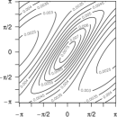
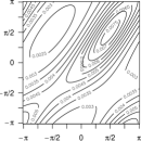
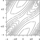
(a)	(b)	(c)	(d)
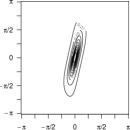
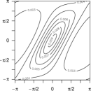
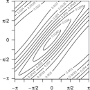
	(e)	(f)	(g)
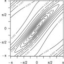
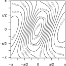
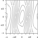
	(h)	(i)	(j)

Figure 1: Contour plots of density (5) with $\rho_{23}=0.1$ and: (a)–(d) $(-\rho_{12},-\rho_{13})=(1,0.5)$ and (a) $u_{3}=0$, (b) $u_{3}=\pi/2$, (c) $u_{3}=\pi$ and (d) $u_{3}=3\pi/2$, (e)–(g) $(-\rho_{13},u_{3})=(0.5,0)$ and (e) $-\rho_{12}=0.15$, (f) $-\rho_{12}=0.6$ and (g) $-\rho_{12}=2.5$, and (h)–(j) $(-\rho_{12},u_{3})=(1,0)$ and (h) $-\rho_{13}=0.25$, (i) $-\rho_{13}=2$ and (j) $-\rho_{13}=5$. The $x$-axis represents the value of $u_{1}$, while the $y$-axis denotes the value of $u_{2}$.

Figure 1 plots the density (5) for fixed values of the third component $u_{3}$ and selected values of the parameters. The frames (a)–(d) imply that the values of $u_{3}$ control the location of $(u_{1},u_{2})$ when the density (5) is viewed as function of $(u_{1},u_{2})$. Also, as visual confirmation of Theorem 7, the modes and antimodes of the density (5) are given at $u_{1}=u_{2}=u_{3}$ and $u_{1}+\pi=u_{2}=u_{3}$, respectively. The comparison among the frames (a) and (e)–(g) suggests that the dependence between $U_{1}$ and $U_{2}$ becomes strong when the parameter $\rho_{12}$ is close to the non-zero or non-infinite boundary of its parameter space. With the fixed values of $\rho_{13}$ and $\rho_{23}$ in the frames (a) and (e)–(g), the range of $\rho_{12}$ is about $|\rho_{12}|\in(0,0.083]\cup[0.124,\infty)$. It can be seen that the closer the value of $|\rho_{12}|$ to 0.124, the greater the dependence between $U_{1}$ and $U_{2}$. In turn, with the fixed values of $\rho_{12}$ and $\rho_{23}$ in the frames (a) and (h)–(j), the range of $\rho_{13}$ is about $|\rho_{13}|\in(0,0.09]\cup[0.11,\infty)$. Although $\rho_{13}$ controls the dependence between $U_{1}$ and $U_{3}$, it can be seen that this parameter indirectly influences the dependence between $U_{1}$ and $U_{2}$. The frames (a) and (h)–(j) suggest that the dependence between $U_{1}$ and $U_{2}$ becomes strong as $|\rho_{13}|$ goes to 0.11.

4 Parameter Estimation

In this section we consider methods of moments estimation and maximum likelihood estimation. Throughout this section, let $\{(U_{1m},U_{2m},U_{3m})\}_{m=1}^{n}$ be a random sample from the distribution (5).

4.1 Method of moments estimation

Method of moments estimators can be obtained by equating theoretical and empirical trigonometric moments

$$E\left\{e^{i(p_{1}U_{1}+p_{2}U_{2}+p_{3}U_{3})}\right\}=\frac{1}{n}\sum_{m=1}^{n}e^{i(p_{1}U_{1m}+p_{2}U_{2m}+p_{3}U_{3m})}$$

for some selected values of $(p_{1},p_{2},p_{3})\in\mathbb{Z}^{3}$. In order to estimate the parameters of the original distribution (5), possible choices of $(p_{1},p_{2},p_{3})$ are $(p_{j},p_{k},p_{\ell})=(1,-1,0)$ with $j<k$. In this case, equations (15) and (33) imply that (following lengthy but simple calculations for the second equality)

$$E\left\{e^{i(U_{j}-U_{k})}\right\}=-\rho_{k\ell}\left(\frac{\varphi_{k\ell}}{\rho_{jk}}+\frac{1}{\rho_{j\ell}}\right)=\varphi_{jk}.$$

It follows that the parameters can be estimated as the solution of the following equations:

$${\hat{\varphi}_{jk}}=\frac{1}{n}\sum_{m=1}^{n}e^{i(u_{jm}-u_{km})},\quad 1\leq j<k\leq 3,$$

where $\hat{\varphi}_{jk}$ is the estimate of $\varphi_{jk}$ defined in Theorem 2(i). Although there is no closed expression for $\{\hat{\rho}_{jk}\}$, it is straightforward to find these estimates numerically thanks to the simple expressions for $\{\hat{\varphi}_{jk}\}$.

4.2 Maximum likelihood estimation (MLE)

For the original model (5), the likelihood function for $\{(u_{m1},u_{m2},u_{m3})\}_{m=1}^{n}$ is given by

$$\log L(\rho_{12},\rho_{13},\rho_{23})=\ \log\prod_{m=1}^{n}c(u_{m1},u_{m2},u_{m3})$$

$$=\ n\log c_{2}-\sum_{m=1}^{n}\log F_{m}.$$ (18)

where $F_{m}=c_{1}+2\{\rho_{12}\cos(u_{m1}-u_{m2})+\rho_{13}\cos(u_{m1}-u_{m3})+\rho_{23}\cos(u_{m2}-u_{m3})\}$. Its score function is

$$\frac{\partial}{\partial\rho_{jk}}\log L(\rho_{12},\rho_{13},\rho_{23})=n\frac{\frac{\partial c_{2}}{\partial\rho_{jk}}}{c_{2}}-\sum_{m=1}^{n}\frac{\frac{\partial c_{1}}{\partial\rho_{jk}}+2\cos(u_{mj}-u_{mk})}{F_{m}}$$

where

$$\frac{\partial c_{1}}{\partial\rho_{jk}}=\frac{\rho_{j\ell}}{\rho_{k\ell}}+\frac{\rho_{k\ell}}{\rho_{j\ell}}-\frac{\rho_{k\ell}\rho_{j\ell}}{\rho_{jk}^{2}},$$

$$\frac{\partial c_{2}}{\partial\rho_{jk}}=\frac{1}{(2\pi)^{3}}\left\{\rho_{jk}\left(\left(\frac{\rho_{j\ell}}{\rho_{k\ell}}\right)^{2}+\left(\frac{\rho_{k\ell}}{\rho_{j\ell}}\right)^{2}\right)-\frac{(\rho_{k\ell}\rho_{j\ell})^{2}}{\rho_{jk}^{3}}-2\rho_{jk}\right\}\left((2\pi)^{3}c_{2}\right)^{-1}.$$

The maximum likelihood estimates $\hat{\rho}_{12},\hat{\rho}_{13},\hat{\rho}_{23}$ are obtained by equating the score function to zero and numerically solving the system of three equations, see below. For the reader’s convenience, we provide in Appendix B the associated expected Fisher information matrix.

Although the proposed density (5) has a simple and closed form, one should be careful about the parameter constraint, namely, $|\rho_{k\ell}|<|\rho_{jk}\rho_{j\ell}|/(|\rho_{jk}|+|\rho_{j\ell}|)$ for some $(j,k,\ell)$. In order to simplify this parameter constraint for numerical optimization, we use the condition for identifiability given in Proposition 2. Assuming that $\rho_{12}\rho_{13}\rho_{23}=1$, the parameter constraint reduces to $|\rho_{jk}|+|\rho_{j\ell}|<|\rho_{jk}|^{2}|\rho_{j\ell}|^{2}$ or, solving an inequality of the second order,

$$|\rho_{jk}|>\frac{1+\{1+4|\rho_{j\ell}|^{3}\}^{1/2}}{2|\rho_{j\ell}|^{2}}.$$

Using the expression

$$\rho_{jk}=\frac{1+\{1+4|\rho_{j\ell}|^{3}\}^{1/2}}{2|\rho_{j\ell}|^{2}}\frac{1}{\zeta_{jk}},\quad\zeta_{jk}\in\left(-1,0\right)\cup\left(0,1\right),$$

it is straightforward to see that the parameters of the proposed model (5) can be expressed in terms of $\rho_{j\ell}$ and $\zeta_{jk}$ alone (remember that this holds for one choice of $j,k,\ell$). The parameter space of this reparametrized model under the constraint $|\rho_{k\ell}|<|\rho_{jk}\rho_{j\ell}|/(|\rho_{jk}|+|\rho_{j\ell}|)$ and $\rho_{12}\rho_{13}\rho_{23}=1$ is thus

$$\tilde{\Omega}=\left\{(\zeta_{jk},\rho_{j\ell})\,;\,\zeta_{jk}\in\left(-1,0\right)\cup\left(0,1\right),\rho_{j\ell}\in\mathbb{R}\setminus\{0\}\right\}.$$

For notational convenience, write $\log L(\rho_{12},\rho_{13},\rho_{23})=\log L(\zeta_{jk},\rho_{j\ell})$ if the log-likelihood function (4.2) is represented in terms of $(\zeta_{jk},\rho_{j\ell})$. Then the maximum likelihood estimation for the proposed model can be carried out as follows:

1. For $(k,\ell)$ successively being equal to $(1,2),(2,3),(3,1)$, obtain the following estimates

   $$(\tilde{\zeta}_{jk},\tilde{\rho}_{j\ell}) =\mathop{\rm arg~{}max}\limits_{(\zeta_{jk},\rho_{j\ell})\in\tilde{\Omega}}\log L(\zeta_{jk},\rho_{j\ell}).$$

2. Among the three obtained maximized quantities, calculate

   $$(\hat{\zeta}_{j^{*}k^{*}},\hat{\rho}_{j^{*}\ell^{*}})=\mathop{\rm arg~{}max}\limits_{(\tilde{\zeta}_{jk},\tilde{\rho}_{j\ell})}\,\log L(\tilde{\zeta}_{jk},\tilde{\rho}_{j\ell}).$$

3. Record the maximum likelihood estimate $(\hat{\rho}_{12},\hat{\rho}_{13},\hat{\rho}_{23})$ as

   $$\hat{\rho}_{j^{*}\ell^{*}}=\hat{\rho}_{j^{*}\ell^{*}},\quad\hat{\rho}_{j^{*}k^{*}}=\frac{1+\{1+4|\hat{\rho}_{j^{*}\ell^{*}}|^{3}\}^{1/2}}{2|\hat{\rho}_{j^{*}\ell^{*}}|^{2}}(2\hat{\zeta}_{j^{*}k^{*}}-1),\quad\hat{\rho}_{k^{*}\ell^{*}}=\frac{1}{\hat{\rho}_{j^{*}k^{*}}\hat{\rho}_{j^{*}\ell^{*}}},$$

   where $j^{*}\neq k^{*}\neq\ell^{*}$.

The algorithm is repeated with different initial values, to make sure that the global maximum is achieved. The initial values for the parameters $\zeta_{jk}$ and $\rho_{j\ell}$ are uniformly chosen from the intervals they are allowed to take values (where of course the infinite intervals for $\rho_{j\ell}$ are limited to a large maximal value). The function for calculating the ML estimates was written in the programming language R, using the optimizer solnp from the library Rsolnp [17] and is available in the GitHub repository https://github.com/Sophia-Loizidou/Trivariate-wrapped-Cauchy-copula. The consistency of this approach is shown and its finite-sample performance is investigated by means of Monte Carlo simulations, which we provide in Supplementary material A and B.

5 Adding specified angular and/or linear marginals to the trivariate wrapped Cauchy copula

Let $(U_{1},U_{2},U_{3})$ be a random vector which follows the trivariate wrapped Cauchy copula (5). Assume that either

• $f_{j}$ is a density on the circle $[0,2\pi)$ $(j=1,2,3)$ and $F_{j}$ its distribution function with fixed and arbitrary origin, namely, $F_{j}(\theta)=\int_{c_{j}}^{\theta}f_{j}(x)dx$ with $c_{j}\in[0,2\pi)$;

• $f_{j}$ is a density on (a subset of) the real line $\mathbb{R}$ $(j=1,2,3)$ and $F_{j}$ its distribution function.

Define

$$(\Theta_{1},\Theta_{2},\Theta_{3})=\left(F_{1}^{-1}\left(\frac{U_{1}}{2\pi}\right),F_{2}^{-1}\left(\frac{U_{2}}{2\pi}\right),F_{3}^{-1}\left(\frac{U_{3}}{2\pi}\right)\right).$$

Then it follows that $(\Theta_{1},\Theta_{2},\Theta_{3})$ has the joint density

$$f(\theta_{1},\theta_{2},\theta_{3})=(2\pi)^{3}c_{2}\Bigl{(}c_{1}+2\sum_{1\leq j<k\leq 3}\rho_{jk}\cos[2\pi\{F_{j}(\theta_{j})-F_{k}(\theta_{k})\}]\Bigr{)}^{-1}\prod_{1\leq\ell\leq 3}f_{\ell}(\theta_{\ell}),$$ (19)

where each $\theta_{j}$ either belongs to $[0,2\pi)$ or to (a subset of) $\mathbb{R}$. As is clear from the definition, the univariate marginal density of $\Theta_{j}$ is given by $f_{j}$  $(j=1,2,3)$. This yields a very flexible class of distributions with either 3 angular components, 2 angular and 1 linear components, 1 angular and 2 linear components, or even 3 linear components. The reason why there is no distinction between the type of marginal lies in the simple fact that the uniform distribution on $[0,2\pi)$ bears by nature a double role as being linear as well as circular (since all points, and in particular the endpoints, share the same value). This unified viewpoint was strangely enough not taken up by the two papers [26] and [64], nor in [29] where the concept of copulas for circular data has been discussed in general. To the best of our knowledge, only [38] combines copulas for angular data with linear marginals.

From the properties of the trivariate wrapped Cauchy copula, we can then derive the following general results (whose proof is omitted).

Theorem 8.

Let $(\Theta_{1},\Theta_{2},\Theta_{3})$ have the density (19). Then the following hold for $(\theta_{1},\theta_{2},\theta_{3})$ each either belonging to $[0,2\pi)$ or to (a subset of) $\mathbb{R}$:

1. The univariate marginal distribution of $\Theta_{j}$ is $f_{j}(\theta_{j})$.

2. The bivariate marginal distribution of $(\Theta_{j},\Theta_{k})$ is

   $$f(\theta_{j},\theta_{k})=4\pi^{2}c(2\pi F_{j}(\theta_{j}),2\pi F_{k}(\theta_{k}))f_{j}(\theta_{j})f_{k}(\theta_{k}),$$

   where $c(\cdot,\cdot)$ is the density (8).

3. The bivariate conditional distribution of $(\Theta_{j},\Theta_{k})$ given $\Theta_{\ell}=\theta_{\ell}$ is

   $$f(\theta_{j},\theta_{k}|\theta_{\ell})=4\pi^{2}c(2\pi F_{j}(\theta_{j}),2\pi F_{k}(\theta_{k})|2\pi F_{\ell}(\theta_{\ell}))f_{j}(\theta_{j})f_{k}(\theta_{k}),$$

   where $c(\cdot,\cdot|\cdot)$ is the density (11).

4. The univariate conditional distribution of $\Theta_{j}$ given $\Theta_{k}=\theta_{k}$ is

   $$f(\theta_{j}|\theta_{k})=2\pi c(2\pi F_{j}(\theta_{j})|2\pi F_{k}(\theta_{k}))f_{j}(\theta_{j}),$$

   where $c(\cdot|\cdot)$ is the density (13).

5. The univariate conditional distribution of $\Theta_{j}$ given $(\Theta_{k},\Theta_{\ell})=(\theta_{k},\theta_{\ell})$ is

   $$f(\theta_{j}|\theta_{k},\theta_{\ell})=2\pi c(2\pi F_{j}(\theta_{j})|2\pi F_{k}(\theta_{k}),2\pi F_{\ell}(\theta_{\ell}))f_{j}(\theta_{j}),$$

   where $c(\cdot|\cdot,\cdot)$ is the density (14).

These results demonstrate that with our new model all forms of regression analysis involving up to three angular and/or linear components are straightforward, which in a single swift covers the needs mentioned in the Introduction. Random number generation from the general model is also immediate by adding just the step

$$\Theta_{j}=F_{j}^{-1}\left(\frac{U_{j}}{2\pi}\right),j=1,2,3,$$

to the algorithm presented in Section 3.2.

We conclude this section by briefly discussing one particular choice of marginals, namely when each $f_{j}$ is the wrapped Cauchy density

$$f_{j}(\theta)=\frac{1}{2\pi}\frac{1-\xi_{j}^{2}}{1+\xi_{j}^{2}-2\xi_{j}\cos(\theta-\mu_{j})},\quad 0\leq\theta<2\pi,$$ (20)

where $\mu_{j}$ is the location parameter and $\xi_{j}\in(-1,1)$ the concentration parameter. Assume that the origin of the distribution function $F_{j}$ is $c_{j}=\mu_{j}$. In this case $F_{j}$ has the closed-form expression

$$F_{j}(\theta_{j})=\frac{1}{\pi}\arctan\left(\frac{1+\xi_{j}}{1-\xi_{j}}\tan\frac{\theta_{j}-\mu_{j}}{2}\right)+I(\theta_{j}>\mu_{j}+\pi),\quad\mu_{j}<\theta_{j}<\mu_{j}+2\pi.$$

Then, noting that $\cos(2\arctan x)=(1-x^{2})/(1+x^{2})$ and $\sin(2\arctan x)=2x/(1+x^{2}),\ x\in\mathbb{R},$ it is a tedious but straightforward exercise to show that the density of (19) can be expressed as

$$f(\theta_{1},\theta_{2},\theta_{3})=c_{2}\prod_{j=1}^{3}(1-\xi_{j}^{2})\Biggl{[}c_{1}\prod_{j=1}^{3}g_{j}(\theta_{j})+2\sum_{\begin{subarray}{c}1\leq k<\ell\leq 3\\ j\neq k,\ell\end{subarray}}\rho_{jk}{g_{\ell}(\theta_{\ell})h_{jk}(\theta_{j},\theta_{k})}\Biggr{]}^{-1},$$ (21)

where $g_{j}(\theta_{j})=1+\xi_{j}^{2}-2\xi_{j}\cos(\theta_{j}-\mu_{j})$ and

$$\begin{split}h_{jk}(\theta_{j},\theta_{k})=\ &(1+\xi_{j}^{2})(1+\xi_{k}^{2})\cos(\theta_{j}-\mu_{j})\cos(\theta_{k}-\mu_{k})\\ &+(1-\xi_{j}^{2})(1-\xi_{k}^{2})\sin(\theta_{j}-\mu_{j})\sin(\theta_{k}-\mu_{k})-2\xi_{k}(1+\xi_{j}^{2})\cos(\theta_{j}-\mu_{j})\\ &-2\xi_{j}(1+\xi_{k}^{2})\cos(\theta_{k}-\mu_{k})+4\xi_{j}\xi_{k}.\end{split}$$

Note that the density (21) does not involve any integrals. As further nice properties derived from Theorem 8, the wrapped Cauchy copula with wrapped Cauchy marginals also has wrapped Cauchy conditionals for $\Theta_{j}$ given $\Theta_{k}=\theta_{k}$ and for $\Theta_{j}$ given $(\Theta_{k},\Theta_{\ell})=(\theta_{k},\theta_{\ell})$. Moreover, the bivariate marginal distribution of $(\Theta_{j},\Theta_{k})$ is the distribution of [35] with density

$$f(\theta_{j},\theta_{k})=\tilde{c}\,\{\tilde{c}_{0}-\tilde{c}_{1}\cos(\theta_{j}-\mu_{j})-\tilde{c}_{2}\cos(\theta_{k}-\mu_{k}) -\tilde{c}_{3}\cos(\theta_{j}-\mu_{j})\cos(\theta_{k}-\mu_{k})$$

$$- \tilde{c}_{4}\sin(\theta_{j}-\mu_{j})\sin(\theta_{k}-\mu_{k})\}^{-1},$$

where $\tilde{c}=(1-\rho_{jk}^{2})(1-\xi_{j}^{2})(1-\xi_{k}^{2})/(4\pi^{2})$, $\tilde{c}_{0}=(1+\rho_{jk}^{2})(1+\xi_{j}^{2})(1+\xi_{k}^{2})-8\rho_{jk}\xi_{j}\xi_{k}$, $\tilde{c}_{1}=2(1+\rho_{jk}^{2})\xi_{j}(1+\xi_{k}^{2})-4\rho_{jk}(1+\xi_{j}^{2})\xi_{k}$, $\tilde{c}_{2}=2(1+\rho_{jk}^{2})(1+\xi_{j}^{2})\xi_{k}-4\rho_{jk}\xi_{j}(1+\xi_{k}^{2})$, $\tilde{c}_{3}=-4(1+\rho_{jk}^{2})\xi_{j}\xi_{k}+2\rho_{jk}(1+\xi_{j}^{2})(1+\xi_{k}^{2})$, and $\tilde{c}_{4}=2\rho_{jk}(1-\xi_{j}^{2})(1-\xi_{k}^{2})$. Random number generation from the distribution (21) is based upon the Möbius transformation

$$\Theta_{j}=F_{j}^{-1}\left(\frac{U_{j}}{2\pi}\right)=\mu_{j}+2\arctan\left[\frac{1-\xi_{j}}{1+\xi_{j}}\tan\left(\frac{U_{j}}{2}\right)\right].$$

6 Comparison with existing models from the literature

After having discussed the main properties of our new copula, we can now proceed to a comparison with respect to the competitors from the literature.

The arguably best-known model is the multivariate von Mises distribution of [47]. Unlike our proposal, the multivariate von Mises has a complicated normalizing constant which is “unknown in any explicit form for $p>2$” (where $p$ is the dimension in their paper), hence in particular in the trivariate case. Quoting [49] on the multivariate sine distribution (a special case of the multivariate von Mises): “However, the use is somewhat hampered beyond the bivariate case as the normalizing constant is intractable”. While the trivariate von Mises has von Mises conditional distributions, the authors say that it does not appear possible to obtain an analytic expression for the univariate marginals, but numerical experiments suggest that the shape is either unimodal or bimodal symmetric, hence less flexible than our model. Parameter estimation is not obvious, and the authors suggest a pseudo-likelihood approach. [58] introduces a computationally optimized version of the full pseudo-likelihood as well as a circular distance to address the problems of the multivariate von Mises distribution. Sampling from the multivariate von Mises distribution can be done with rejection sampling for small dimension and with Gibbs sampler for higher dimensions, implying that it is computationally expensive to obtain samples. In [49] a concentrated multivariate sine model is introduced as a special case of the multivariate von Mises. The main idea is to approximate the normalizing constant when the sine distribution is concentrated. However, certain conditions need to be satisfied for the approximation to be good and the approximation is compared to the true normalising constant only in the univariate and bivariate cases.

[54] introduced the multivariate Generalised von Mises (mGvM) distribution which is a maximum entropy distribution just like its von Mises counterpart. It also shares the fact of not admitting an analytic expression for its normalizing constant, which is a major drawback as it forces the use of approximate inference techniques. Its univariate conditionals are Generalised von Mises, but no form is available for marginals. Furthermore a Gibbs sampler is required for simulating from the distribution.

The multivariate wrapped normal distribution dates back to [4]. Its log-likelihood involves (multiple) infinite sums due to an intractable normalizing constant, so alternative methods are required for estimating its parameters. [56] proposes two estimation procedures based on Expectation-Maximisation and Classification Expectation-Maximisation algorithms for estimating the parameters of a multivariate wrapped normal distribution. The two proposed methods can also be used for estimating parameters in the case of joint circular and linear variables, with the circular part being wrapped normal and the linear part normal. Unsurprisingly, the model thus inherits tractability issues from the univariate wrapped normal, which is therefore sometimes approximated by a von Mises. On a related note, [27] formulates a wrapped Gaussian spatial process model where Markov Chain Monte Carlo is required for fitting the model.

[52] proposes the joint projected and skew normal distribution which is a multivariate circular-linear distribution. The distribution models dependence among the components, has mostly interpretable parameters and a random number generation mechanism. However, it inherits from the projected normal distribution the impossibility to express the density in closed form as soon as the circular dimension is larger than 1. Moreover, a non-identifiability issue forces a Bayesian framework and implementation of Markov Chain Monte Carlo Gibbs sampler for obtaining posterior samples. In the paper, 30.000 observations are used as the burn-in period, which indicates that the sampler is computationally expensive.

A $d$-dimensional copula for toroidal data has been proposed in [37] by directly extending the copula construction (2) to

$$f(\theta_{1},\theta_{2},\ldots,\theta_{k})=(2\pi)^{m}\prod_{j=1}^{m}\left\{g\left[2\pi\sum_{i=j}^{k}F_{i}(\theta_{i})\right]\right\}\prod_{i=1}^{k}f_{i}(\theta_{i})$$

where $1\leq m\leq k-1$ and the $f_{i}$ and $F_{i}$, $i=1,\ldots,k$, are respectively circular density and distribution functions. Their suggested three-dimensional copula corresponds to $k=3$ and $m=1$. Being a copula, this model comes closest to ours in terms of flexibility. The authors investigate various inferential properties and show that the conditional distributions are of the same form as the general copula. Their model lacks symmetry concerning the permutation of variables when $m>1$; specifically, $f(\theta_{i},\theta_{j},\theta_{k})$ and $f(\theta_{k},\theta_{i},\theta_{j})$ represent essentially different models. Further properties such as moments, modality, identifiability, bivariate marginal distributions, random number generation, ease of parameter estimation, parameter interpretability are not discussed and hence difficult to evaluate. The authors also do not provide suggestions as to which combinations of marginals and copula $g$ are viable. A real data comparison from [37] reveals that, in terms of AIC, the model chosen by the authors provided a less good fit than the MNNTS which we describe last.

[9] proposes the multivariate nonnegative trigonometric sums (MNNTS) models. The properties of the MNNTS models are studied in [11], who state that the main drawback of the models is the high number of parameters. Marginal and conditional distributions as well as moment expressions are available. Maximum likelihood estimates of the parameters can be calculated using a Newton-like algorithm on the surface of a hypersphere, and a rejection algorithm allows simulating data.

Based on this discussion, the MNNTS model comes closest to our proposal in terms of properties and practical applicability, which is why we consider it as competitor in a real data analysis for trivariate circular data in the following section. Note that besides the very short Section 3.3 in [56] no paper discusses both trivariate angular and angular-linear models.

7 Application on real world datasets

7.1 Protein data

Predicting the 3D structure of proteins is a critical area of research in bioinformatics and computational biology. A groundbreaking advance has been made by Google DeepMind’s AlphaFold [30] which can very accurately predict this folding by means of well-trained deep neural networks. Consequently, in September 2023, two researchers from this team were awarded the prestigious Lasker science prize, which raises the prospect of their team winning potentially also a Nobel prize. Their approach thus solves, in a sense, the single structure point prediction, but it does not allow for uncertainty quantification. As mentioned in the recent Nature Methods paper [40], “distributions of conformations are the future of structural biology” because single-structure views are not able to capture all protein functions. The main body of statistical research in this direction has so far concentrated on the two dihedral angles of amino acids, which has already led to various contributions in the protein structure prediction problem, see for instance [5], [20], [13], or the monograph [19] and Chapters 1 and 4 of [43]. With our trivariate wrapped Cauchy copula, we can contribute to this essential issue and hence complement the AI developments by modelling the dihedral angles as well as the torsion angle of the side chain $\omega$.

The building blocks of proteins are the amino acids, which consist of the backbone and the sidechains. The backbone consists of the chemical bonds NH-C$\alpha$ and C$\alpha$-CO, where C$\alpha$ denotes the central Carbon atom. The aforementioned bonds can rotate around their axes, with $\phi$ denoting the NH-C$\alpha$ torsion angle and $\psi$ the C$\alpha$-CO angle. These angles need to be studied as specific combinations of them allow the favourable hydrogen bonding patterns, while others can ‘result in clashes within the backbone or between adjacent sidechains’ [21]. The $\omega$ angle denotes the N-C torsion angle, where C is the non-central carbon atom. The angle $\omega$ can only take the values $0$ and $\pi$, and for previous works this angle was considered to be fixed at one of the two values [3, 20]. However, in practice this angle is often measured with some noise and using our distribution (5), we shall model all three angles.

For the present data analysis, we consider position 55 at 2000 randomly selected times in the molecular dynamic trajectory of the SARS-CoV-2 spike domain from [16]. The position occurs in $\alpha$-helix throughout the trajectory. DPPS [32] is used to compute the secondary structure and [6] to verify the chains. As can be seen from Figure 2, the marginal distributions of the data cannot be modelled by the uniform distribution on the circle, so other distributions need to be explored. Conveniently, our trivariate wrapped Cauchy copula allows us to choose different marginals, which is why we combined it respectively with wrapped Cauchy, cardioid, von Mises and Kato–Jones marginals. Of course, many other choices are possible, and one can also combine distinct marginals. Alternatively, it is also viable to estimate the marginals in a non-parametric way and then combine the estimated marginals with our copula (see [15] for such a procedure in $\mathbb{R}^{d}$).

Figure 2: Rose plots of the protein data. The marginals are not uniformly distributed on the circle.

The parameters of our models are estimated using MLE. In the case that the marginal distributions are not uniform, the maximum likelihood estimates of the parameters are calculated in a two-step approach. Let $\{(\theta_{m1},\theta_{m2},\theta_{m3})\}_{m=1}^{2000}$ denote the sequence of toroidal observations. In the first step, the ML estimates of the parameters of the marginals are calculated, followed in the second step by estimating the parameters of the copula using $\{u_{1m},u_{2m},u_{3m}\}_{m=1}^{2000}$ for

$$(u_{1m},u_{2m},u_{3m})=\Bigl{(}2\pi F_{1}(\theta_{1m};\hat{\vartheta}_{1}),2\pi F_{2}(\theta_{2m};\hat{\vartheta}_{2}),2\pi F_{3}(\theta_{3m};\hat{\vartheta}_{3})\Bigr{)},$$

where, for $i\in\{1,2,3\}$, $F_{i}$ represents the marginal density function of $\theta_{i}$ and $\hat{\vartheta}_{i}$ the parameters obtained from the first step of the maximization. [23] refers to this as the method of inference functions for margins or IFM method. Efficiency and consistency of the estimates obtained with IFM compared to the estimates that can be obtained by performing one maximisation of the likelihood function can be found in Chapter 10 of [23] and Chapter 5 of [24].

As plotting all three angles at the same time is not possible, Figure 3 shows the plots of the data of two of the angles given the third one. The values of the fixed angles are chosen to be the mode of the data, and only points that are within 0.1 radians of chosen value of the fixed angle are plotted. In order to make the plots clearer, the range of values on each axis is not between $0$ and $2\pi$, like the traditional Ramachandran plot, but it is chosen such that both the contour plots and the points are visible. For the values of $\omega$, most observations were around 0 and so the plot is translated from $[0,2\pi$) to $[-\pi,\pi)$ such that making the range of values on the axis smaller is possible. The contour plots correspond to our copula density (5) with the marginal distributions being the von Mises distribution, whose density is given by

$$f(\theta)=\frac{1}{2\pi I_{0}(\kappa)}\exp^{\kappa\cos(\theta-\mu)},\quad\theta\in[0,2\pi),$$ (22)

where $I_{0}(\kappa)$ denotes the modified Bessel function of the first kind and order 0. The von Mises marginals with their lighter tails lead to the best fit for this concentrated dataset, as measured by both Akaike and Bayesian Information Criteria, see Table 1 (a force of our flexible model is that other marginals will be more adapted to less concentrated data). The observed data points are plotted on top of the contours. This gives a visual idea of how good our estimated model fits the protein data. The inherent tractability of our model allows biologists and bioinformaticians to quantify uncertainties, compute quantities of interest, and in particular our straightforward random number generation process enables them to quickly simulate data from our model, which is essential in their pipelines [63].

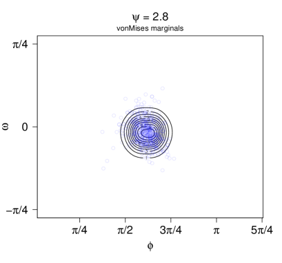
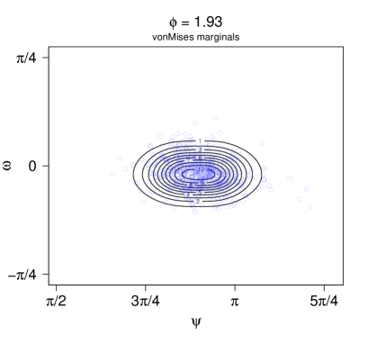
Figure 3: Contour plots of density (5) with von Mises marginals, with parameter values estimated by maximum likelihood. The parameters of the marginals are $\hat{\mu}_{1}=1.93,\hat{\kappa}_{1}=27.6,\hat{\mu}_{2}=2.82,\hat{\kappa}_{2}=17.3,\hat{\mu}_{3}=6.23,\hat{\kappa}_{3}=84.4$, where $\hat{\mu}_{i}$ and $\hat{\kappa}_{i}$ denote the estimated value for $\mu$ and $\kappa$ of density (22) corresponding to the marginal distribution of $\theta_{i}$ for $i\in\{1,2,3\}$, and the copula parameters are $\hat{\rho}_{12}=9.18,\hat{\rho}_{13}=-1.17,\hat{\rho}_{12}=-0.09$.

We conclude this section by a comparison of our model with the trivariate non-negative trigonometric sums (MNNTS) distribution of [9]. Table 1 presents the fit of various models. The maximised log-likelihood, AIC and BIC are reported for each model, along with the number of free parameters, denoted by $p$. The algorithms for fitting the MNNTS distribution are taken from the R package CircNNTS [10]. Besides the reasons mentioned in Section 6 to compare our model to the MNNTS, it is also the only competitor for which we could find implemented and working code. The number of free parameters for MNNTS($M_{1},M_{2},M_{3}$) is calculated as $2\left(\prod_{i=1}^{3}(M_{i}+1)-1\right)$. Various combinations of the values $M_{1},M_{2},M_{3}$ are shown in Table 1, with the number of free parameters increasing rapidly. The MNNTS is not able to match the fit of our copula (not only in terms of AIC/BIC but even in terms of log-likelihood), even for a very large number of parameters. The best model for all three measures of fit, the trivariate wrapped Cauchy copula with von Mises marginals, is shown in bold.

Table 1: Maximized log-likelihood, AIC, BIC, and the number of free parameters (denoted by $p$) for each model for the protein dataset.

Model	Marginals	log-likelihood	AIC	BIC	$p$
	uniform	-7920	15845	15862	2
trivariate wrapped	wrapped Cauchy	1131	-2245	-2194	8
Cauchy copula	cardioid	-3495	7007	7058	8
	von Mises	2046	-4074	-4023	8
	Kato–Jones	1404	-2778	-2694	14
	($M_{1},M_{2},M_{3}$)
	(0,0,0)	-11027	22055	22055	0
	(1,1,1)	-6923	13874	13953	14
	(2,2,2)	-4582	9268	9559	52
	(3,3,3)	-2984	6220	6926	126
MNNTS	(4,4,4)	-1811	4118	5507	248
	(5,5,5)	-921	2702	5111	430
	(6,6,6)	-231	1829	5660	684
	(7,7,7)	315	1414	7138	1022
	(8,8,8)	746	1421	9575	1456
	(9,9,9)	1091	1815	13005	1998
	(10,10,10)	1370	2579	17478	2660

7.2 Wave data

For the second real data application, we use a time series of 1326 observations of semi-hourly wave directions and heights, recorded in the period 15/02/2010–16/03/2010 by the buoy of Ancona, located in the Adriatic Sea at about 30 km from the coast. The data points are collected far spaced enough from each other to be considered independent. In order to address the problem mentioned in the Introduction and to consider a more complete picture than just wave height (linear) and direction (circular), we also add the wind direction (circular). The data thus is hyper-cylindrical, which we can perfectly analyze with our copula. We choose as circular marginals the wrapped Cauchy distribution and the Weibull distribution for the linear marginal. Of course, many other combinations could be considered, but this goes beyond the scope of the present paper. Due to the multimodality of the data, a mixture model is required, leading to densities of the form

$$f(\theta_{1},\theta_{2},x)=\sum_{i=1}^{K}\pi_{i}f_{i}(\theta_{1},\theta_{2},x),\quad\sum_{i=1}^{K}\pi_{i}=1,$$ (23)

where $K$ is the number of components of the mixture model, $\pi_{i}$ is the weight of each class and $f_{i}(\theta_{1},\theta_{2},x)$ is the density of component $i$ and is the copula as defined in (19), with marginals as already explained. In order to estimate the parameters, we use a variant of the Expectation-Maximization (EM) algorithm to find the values of the parameters for each component of the mixture model. As with maximum likelihood estimation with non-uniform marginals, the maximisation is done as a first step for the parameters of the marginal distributions and then, using the obtained parameters, estimates of the parameters of the copula are obtained. The M-step of our algorithm thus adopts the IFM method, which is why we speak of a variant of the EM algorithm, which for the rest works exactly like an EM algorithm. The initial values for the parameters were randomly chosen. This was repeated 10 times and the parameters that maximised the log-likelihood were chosen. To find the number of mixture components, we considered the values $K=2,3,4,5$ and used the BIC to determine the best-fitting model.

We found that $K=4$ components fit best the data, as the BIC values are 16045, 15850, 15611 and 15655, for $K=2,3,4,5$ respectively. The parameter estimates for this mixture model are given in Table 2. For visualization of the results, the bivariate marginal distribution is plotted in Figure 4, as given in Theorem 8. The plots on the left hand side are scatter plots of the data, coloured according to their cluster as given by our variant of the EM algorithm with 4 components. The same colour is used for each cluster to plot the bivariate marginal distribution for each of the components. This fitted model then allows building regression models within each cluster and expressing, for instance, how wave height and direction are influenced by the wind direction or how the wave height depends on both wind and wave direction. The simplicity of our copula is tailor-made for this type of investigations and can provide environmental agencies with a user-friendly tool.

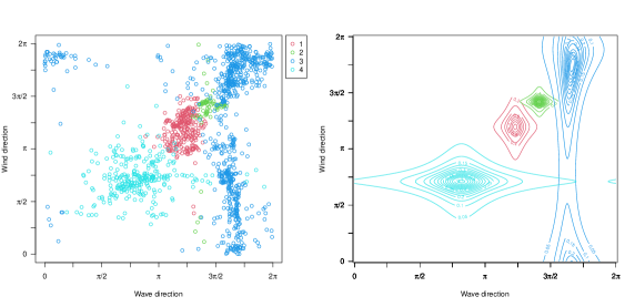
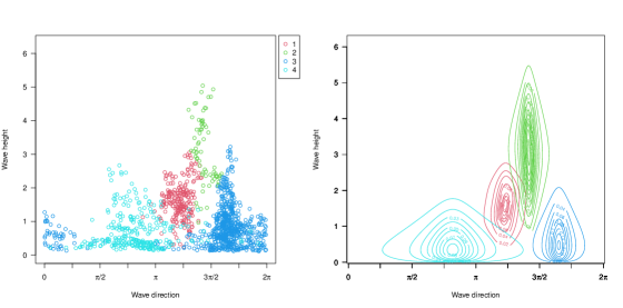
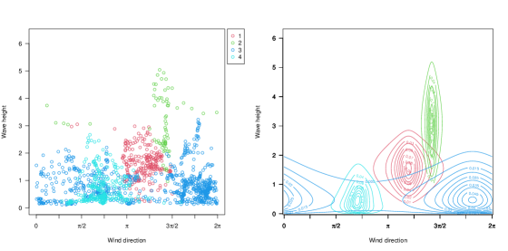
Figure 4: Contour plots of the bivariate marginal distributions for the four different clusters as detected by our variant of the EM algorithm. Each cluster is presented in a different colour.

Table 2: Parameter estimates as obtained from our variant of the EM algorithm for 4 components. The marginal distributions for wind and wave directions are wrapped Cauchy, and the estimates of the parameters are denoted by $\hat{\rho}_{1},\hat{\mu}_{1}$ and $\hat{\rho}_{2},\hat{\mu}_{2}$, respectively. For the Weibull distribution, $\hat{\lambda}_{3}$ is the scale parameter and $\hat{\kappa}_{3}$ is the shape parameter. Finally $\hat{\pi}_{i}$ denotes the estimate of the weight of class $i$.

Parameters	Cluster 1	Cluster 2	Cluster 3	Cluster 4
$\hat{\rho}_{12}$	-0.001	-0.090	-495	0.004
$\hat{\rho}_{13}$	0.010	-0.004	-0.113	3720
$\hat{\rho}_{23}$	-120898	3176	0.018	-0.066
$\hat{\rho}_{1}$	3.866	4.443	5.186	2.572
$\hat{\mu}_{1}$	0.829	0.883	0.804	0.599
$\hat{\rho}_{2}$	3.759	4.463	5.693	2.233
$\hat{\mu}_{2}$	0.723	0.892	0.434	0.768
$\hat{\lambda}_{3}$	3.044	3.380	1.521	1.438
$\hat{\kappa}_{3}$	1.768	3.425	0.941	0.773
$\hat{\pi}_{i}$	0.187	0.053	0.532	0.227

8 Final comments and outlook on future research

In this paper we have proposed a new distribution on the three-dimensional torus, the trivariate wrapped Cauchy copula. The marginal and conditional distributions of the copula are known distributions and random variate generation is simple and efficient through a transformation of uniform random variates without rejection. The proposed distribution is unimodal for any value of the parameters $\rho_{12},\rho_{13}$ and $\rho_{23}$, a very important and rare property in hypertoroidal distributions. Parameter estimation can be performed via maximum likelihood estimation. As the distribution is a copula, the marginal distributions of the components can be chosen as any univariate angular or linear distributions. Choosing marginal distributions that are defined on the real line allows the copula to also model data that do not have all three components as angular variables. This was done for the second real data example, where mixture models were fitted to data that include one linear and two angular variables.

The trivariate wrapped Cauchy copula can be extended in various directions, of which we shall briefly outline three. First, we might wish to introduce asymmetry into our copula (5). Of course, asymmetry can be handled at the level of the marginals via suitably choosing skew marginal distributions, but this does not allow altering the symmetry of the dependence structure, hence the copula itself. This can be done by adopting the approach of [3] which consists in multiplying (5) with the skewing function $(1+\lambda_{1}\sin(u_{1})+\lambda_{2}\sin(u_{2})+\lambda_{3}\sin(u_{3}))$ for $\lambda_{1},\lambda_{2},\lambda_{3}\in(-1,1)$ satisfying $|\lambda_{1}+\lambda_{2}+\lambda_{3}|<1$. When all three skewness parameters are 0, we retrieve the original copula, and as soon as one parameter deviates from zero, we obtain an asymmetric version of (5). It will be interesting to see in how far asymmetry in the copula can add flexibility on top of asymmetry in the marginals, and how both can be ideally combined.

Second, in a similar manner as in [64], the extended model (19) can be applied to presenting an AR(2) process on the circle. Let $\Theta_{0},\Theta_{1},\ldots,\Theta_{t}$ be $[0,2\pi)$-valued random variables on the circle such that

$$p(\theta_{0},\theta_{1}) =f(\theta_{0},\theta_{1}),$$

$$p(\theta_{t}|\theta_{t-1},\ldots,\theta_{0}) =p(\theta_{t}|\theta_{t-1},\theta_{t-2})=\frac{|1-\delta_{t}^{2}|}{1+\delta_{t}^{2}-2\delta_{t}\cos(2\pi F(\theta_{t})-\eta_{t})}f(\theta_{t}),$$ (24)

where $f(\theta_{0},\theta_{1})$ is a density on the torus $[0,2\pi)^{2}$, $f(\theta)$ is a density on the circle $[0,2\pi)$ and $F(\theta)=\int_{c}^{\theta}f(x)dx$ for some arbitrary origin $c$ on the circle. Also, $\eta_{t}=\arg(\phi_{t}),$ $\delta_{t}=|\phi_{t}|,$ $\phi_{t}=-\rho_{t-1,t-2}\{\rho_{t,t-1}^{-1}e^{2\pi iF(\theta_{t-1})}+\rho_{t,t-2}^{-1}e^{2\pi iF(\theta_{t-2})}\}$. The parameters satisfy $\rho_{t,t-1},\rho_{t,t-2},\rho_{t-1,t-2}\in\mathbb{R}$, $\rho_{t,t-1}\cdot\rho_{t,t-2}\cdot\rho_{t-1,t-2}>0$, and $|\rho_{k\ell}|<|\rho_{jk}\rho_{j\ell}|/(|\rho_{jk}|+|\rho_{j\ell}|)$ for $(j,k,\ell)$ a permutation of $(t,t-1,t-2)$. Then $p(\theta_{0},\theta_{1})$ is the initial distribution and $p(\theta_{t}|\theta_{t-1},\theta_{t-2})$ is the stationary transition density, inherited from our trivariate construction. If $f$ is the wrapped Cauchy density (20), then the transition density (24) can also be expressed in closed form without integrals. The nice properties of our model, especially its high tractability, shall make the AR(2) process very appealing and important for time-dependent directional data.

Third and finally, it is natural albeit highly challenging to extend the model presented here to any $d$-dimensional torus. A potential model could be of the form

$$c(u_{1},\ldots,u_{d})\propto\left\{c_{4}+2\sum_{1\leq j<k\leq d}\rho_{jk}\cos(u_{j}-u_{k})\right\}^{-1}$$ (25)

where the parameters $\rho_{jk}\in\mathbb{R}$ need to satisfy certain conditions and $c_{4}$ depends on them. To make this a valid density, $c_{4}$ has at least to be equal to $2\sum_{1\leq j<k\leq d}|\rho_{jk}|$, and we need to find the normalizing constant. The proposal (25) is not only a logical extension of our trivariate copula, but it is also based on the following nice theoretical result (see Appendix A.9 for the proof).

Theorem 9.

Let a $[0,2\pi)^{d}$-valued random vector $(U_{1},\ldots,U_{d})$ have the probability density function $f(u_{1},\ldots,u_{d})$. Suppose that $f$ is a function of $\{u_{j}-u_{k}\,;\,1\leq j<k\leq d\}$, namely,

$$f(u_{1},\ldots,u_{d})=h(u_{1}-u_{2},u_{1}-u_{3},\ldots,u_{d-1}-u_{d}),\quad 0\leq u_{1},\ldots,u_{d}<2\pi.$$

Then the marginal distribution of $U_{j}$ $(1\leq j\leq d)$ has the uniform distribution on the circle.

This desirable result for a copula motivates researching in the direction of density (25).

Appendix

Appendix A Proofs

A.1 Technical lemmas

Lemma 1.

For real-valued variables $\phi_{1},\phi_{2},\phi_{3}$, we have that $|\phi_{j}|>|\phi_{k}|+|\phi_{\ell}|$ for $(j,k,\ell)$ a certain permutation of $(1,2,3)$ if and only if $\phi_{1}z_{1}+\phi_{2}z_{2}+\phi_{3}z_{3}\neq 0$ for all $(z_{1},z_{2},z_{3})\in\Omega^{3}.$

Proof.

Let us start with the necessary condition. Without loss of generality, assume that $|\phi_{1}|>|\phi_{2}|+|\phi_{3}|$. Then the (reverse) triangular inequality combined with straightforward calculations yields

$$|\phi_{1}z_{1}+\phi_{2}z_{2}+\phi_{3}z_{3}| \geq ||\phi_{1}z_{1}|-|\phi_{2}z_{2}+\phi_{3}z_{3}||$$

$$= ||\phi_{1}|-|\phi_{2}z_{2}+\phi_{3}z_{3}||$$

$$= |\phi_{1}|-|\phi_{2}z_{2}+\phi_{3}z_{3}|$$

$$\geq |\phi_{1}|-(|\phi_{2}|+|\phi_{3}|)$$

$$> 0.$$

The sufficient condition requires some more steps. Without loss of generality assume that $\min\{\phi_{1},\phi_{2},\phi_{3}\}=\phi_{1}$. Then $z_{1}\neq-\frac{\phi_{2}z_{2}+\phi_{3}z_{3}}{\phi_{1}}$ and $|\phi_{j}/\phi_{1}|>1$ for $j=2,3$. From the former condition we can deduce that $\left|-\frac{\phi_{2}z_{2}+\phi_{3}z_{3}}{\phi_{1}}\right|<1$ or $\left|-\frac{\phi_{2}z_{2}+\phi_{3}z_{3}}{\phi_{1}}\right|>1$ for all $z_{2},z_{3}\in\Omega^{2}$. The special choices $z_{2}={\rm sgn}(\phi_{2}/\phi_{1})\in\Omega$ and $z_{3}={\rm sgn}(\phi_{3}/\phi_{1})\in\Omega$ lead to

$$\left|-\frac{\phi_{2}z_{2}+\phi_{3}z_{3}}{\phi_{1}}\right|=\left|\frac{\phi_{2}}{\phi_{1}}\right|+\left|\frac{\phi_{3}}{\phi_{1}}\right|>1$$

by our second deduction above. Therefore $\left|-\frac{\phi_{2}z_{2}+\phi_{3}z_{3}}{\phi_{1}}\right|>1$ for all $z_{2},z_{3}\in\Omega^{2}$. Now choose again $z_{2}={\rm sgn}(\phi_{2}/\phi_{1})\in\Omega$ but this time $z_{3}=-{\rm sgn}(\phi_{3}/\phi_{1})\in\Omega$. From our established inequality we thus know that for these choices of $z_{2},z_{3}$

$$\left|-\frac{\phi_{2}z_{2}+\phi_{3}z_{3}}{\phi_{1}}\right|>1$$

$$\Leftrightarrow \left|\left|\frac{\phi_{2}}{\phi_{1}}\right|-\left|\frac{\phi_{3}}{\phi_{1}}\right|\right|>1,$$

and consequently either $|\phi_{2}|>|\phi_{1}|+|\phi_{3}|$ or $|\phi_{3}|>|\phi_{1}|+|\phi_{2}|$. ∎

A.2 Proof of Theorem 1

Proof.

In order to prove the theorem, it suffices to see that the function (5) satisfies: (i) $c(u_{1},u_{2},u_{3})\geq 0$ for any $(u_{1},u_{2},u_{3})$ and (ii) $\int_{[0,2\pi)^{3}}c(u_{1},u_{2},u_{3})du_{1}du_{2}du_{3}=1$.

Proof of (i): Without loss of generality, assume $|\rho_{12}|<|\rho_{13}\rho_{23}|/(|\rho_{13}|+|\rho_{23}|)$. We note that

$$c_{1}+2\left\{\rho_{12}\cos(u_{1}-u_{2})+\rho_{13}\cos(u_{1}-u_{3})+\rho_{23}\cos(u_{2}-u_{3})\right\}$$

$$=\left\|\phi_{1}\begin{pmatrix}\cos u_{1}\\ \sin u_{1}\end{pmatrix}+\phi_{2}\begin{pmatrix}\cos u_{2}\\ \sin u_{2}\end{pmatrix}+\phi_{3}\begin{pmatrix}\cos u_{3}\\ \sin u_{3}\end{pmatrix}\right\|^{2},$$

where $\phi_{j}=\mbox{sgn}(\rho_{k\ell})(\rho_{jk}\rho_{j\ell}/\rho_{k\ell})^{1/2}$, $1\leq j,k,\ell\leq 3$, $k,\ell\neq j$, $k<\ell$. Then

$$\left\|\phi_{1}\begin{pmatrix}\cos u_{1}\\ \sin u_{1}\end{pmatrix}+\phi_{2}\begin{pmatrix}\cos u_{2}\\ \sin u_{2}\end{pmatrix}+\phi_{3}\begin{pmatrix}\cos u_{3}\\ \sin u_{3}\end{pmatrix}\right\|$$

$$\geq\left\|\phi_{3}\begin{pmatrix}\cos u_{3}\\ \sin u_{3}\end{pmatrix}\right\|-\left\|\phi_{1}\begin{pmatrix}\cos u_{1}\\ \sin u_{1}\end{pmatrix}+\phi_{2}\begin{pmatrix}\cos u_{2}\\ \sin u_{2}\end{pmatrix}\right\|$$

$$\geq\sqrt{\frac{\rho_{13}\rho_{23}}{\rho_{12}}}-\left(\sqrt{\frac{\rho_{12}\rho_{13}}{\rho_{23}}}+\sqrt{\frac{\rho_{12}\rho_{23}}{\rho_{13}}}\right)$$

$$>0.$$ (26)

The last inequality follows by showing

$$\frac{\rho_{13}\rho_{23}}{\rho_{12}}-\left(\sqrt{\frac{\rho_{12}\rho_{13}}{\rho_{23}}}+\sqrt{\frac{\rho_{12}\rho_{23}}{\rho_{13}}}\right)^{2}$$

$$=\frac{1}{\rho_{12}\rho_{13}\rho_{23}}\left\{\rho_{13}^{2}\rho_{23}^{2}-\rho_{12}^{2}(|\rho_{13}|+|\rho_{23}|)^{2}\right\}$$

$$>\frac{1}{\rho_{12}\rho_{13}\rho_{23}}\left\{\rho_{13}^{2}\rho_{23}^{2}-\left(\frac{|\rho_{13}\rho_{23}|}{|\rho_{13}|+|\rho_{23}|}\right)^{2}(|\rho_{13}|+|\rho_{23}|)^{2}\right\}$$

$$=0.$$

Therefore $c_{1}+2\left\{\rho_{12}\cos(u_{1}-u_{2})+\rho_{13}\cos(u_{1}-u_{3})+\rho_{23}\cos(u_{2}-u_{3})\right\}>0$ for any $(u_{1},u_{2},u_{3})$.

Next we show that the radicand in $c_{2}$ is positive. It is straightforward to see that

$$\begin{split}\hbox to0.0pt{$\displaystyle\rho_{12}^{2}\rho_{13}^{2}\rho_{23}^{2}\left(\left(\frac{\rho_{12}\rho_{13}}{\rho_{23}}\right)^{2}+\left(\frac{\rho_{12}\rho_{23}}{\rho_{13}}\right)^{2}+\left(\frac{\rho_{13}\rho_{23}}{\rho_{12}}\right)^{2}-2\rho_{12}^{2}-2\rho_{13}^{2}-2\rho_{23}^{2}\right)$\hss}\hskip 28.45274pt\\ &=(\rho_{12}^{2}-\rho_{23}^{2})^{2}\left\{\rho_{13}^{2}-\frac{\rho_{12}^{2}\rho_{23}^{2}(\rho_{12}^{2}+\rho_{23}^{2})}{(\rho_{12}^{2}-\rho_{23}^{2})^{2}}\right\}^{2}-\frac{4\rho_{12}^{6}\rho_{23}^{6}}{(\rho_{12}^{2}-\rho_{23}^{2})^{2}}.\end{split}$$ (27)

It follows from the assumption $|\rho_{12}|<|\rho_{13}\rho_{23}|/(|\rho_{13}|+|\rho_{23}|)$ that $|\rho_{13}|>|\rho_{12}\rho_{23}|/(|\rho_{23}|-|\rho_{12}|)$. Also

$$\rho_{13}^{2}>\left(\frac{|\rho_{12}\rho_{23}|}{|\rho_{23}|-|\rho_{12}|}\right)^{2}.$$

Then the radicand (27) can be evaluated as

$$(\rho_{12}^{2}-\rho_{23}^{2})^{2}\left\{\rho_{13}^{2}-\frac{\rho_{12}^{2}\rho_{23}^{2}(\rho_{12}^{2}+\rho_{23}^{2})}{(\rho_{12}^{2}-\rho_{23}^{2})^{2}}\right\}^{2}-\frac{4\rho_{12}^{6}\rho_{23}^{6}}{(\rho_{12}^{2}-\rho_{23}^{2})^{2}}$$

$$>(\rho_{12}^{2}-\rho_{23}^{2})^{2}\left\{\left(\frac{|\rho_{12}\rho_{23}|}{|\rho_{23}|-|\rho_{12}|}\right)^{2}-\frac{\rho_{12}^{2}\rho_{23}^{2}(\rho_{12}^{2}+\rho_{23}^{2})}{(\rho_{12}^{2}-\rho_{23}^{2})^{2}}\right\}^{2}-\frac{4\rho_{12}^{6}\rho_{23}^{6}}{(\rho_{12}^{2}-\rho_{23}^{2})^{2}}$$

$$=0.$$

Hence $c_{2}>0$. Thus the function (5) satisfies the condition (i) for $|\rho_{12}|<|\rho_{13}\rho_{23}|/(|\rho_{13}|+|\rho_{23}|)$. Due to the symmetry of the function (5), it immediately follows that the condition (i) holds for the other two cases $|\rho_{13}|<|\rho_{12}\rho_{23}|/(|\rho_{12}|+|\rho_{23}|)$ and $|\rho_{23}|<|\rho_{12}\rho_{13}|/(|\rho_{12}|+|\rho_{13}|)$.

Proof of (ii): In order to see that the function (5) satisfies (ii), we first note the equation (3.613.2.6) of [18], that is,

$$\int_{0}^{2\pi}\frac{du}{1+b\cos u}=\frac{2\pi}{|1-b^{2}|^{1/2}},\quad|b|<1.$$ (28)

Using this result, it follows that

$$\int_{0}^{2\pi}c(u_{1},u_{2},u_{3})du_{3}$$

$$=\int_{0}^{2\pi}c_{2}\Bigl{[}c_{1}+2\left\{\rho_{12}\cos(u_{1}-u_{2})+\rho_{13}\cos(u_{1}-u_{3})+\rho_{23}\cos(u_{2}-u_{3})\right\}\Bigr{]}^{-1}du_{3}$$

$$=\frac{c_{2}}{c_{1}+2\rho_{12}\cos(u_{1}-u_{2})}\int_{0}^{2\pi}\left[1+\frac{2\{\rho_{13}\cos(u_{1}-u_{3})+\rho_{23}\cos(u_{2}-u_{3})\}}{c_{1}+2\rho_{12}\cos(u_{1}-u_{2})}\right]^{-1}du_{3}$$

$$=\frac{c_{2}}{c_{1}+2\rho_{12}\cos(u_{1}-u_{2})}\int_{0}^{2\pi}\frac{1}{1+b^{\prime}\cos(u_{3}-a^{\prime})}du_{3}$$

$$=\frac{c_{2}}{c_{1}+2\rho_{12}\cos(u_{1}-u_{2})}\cdot\frac{2\pi}{|1-b^{\prime 2}|^{1/2}},$$ (29)

where $b^{\prime}=2\{\rho_{13}^{2}+\rho_{23}^{2}+2\rho_{13}\rho_{23}\cos(u_{1}-u_{2})\}^{1/2}/\{c_{1}+2\rho_{12}\cos(u_{1}-u_{2})\}$ and $a^{\prime}$ satisfies $\tan\alpha^{\prime}=(\rho_{13}\sin u_{1}+\rho_{23}\sin u_{2})/(\rho_{13}\cos u_{1}+\rho_{23}\cos u_{2})$. The third equality follows from the formula $\alpha\cos u_{3}+\beta\sin u_{3}=\sqrt{\alpha^{2}+\beta^{2}}\cos(u_{3}-\gamma)$, where $\gamma$ satisfies $\tan\gamma=\beta/\alpha$ and the fact that we can write

$$\rho_{13}\cos(u_{1}-u_{3})+\rho_{23}\cos(u_{2}-u_{3})=\cos(u_{3})(\rho_{13}\cos(u_{1})+\rho_{23}\cos(u_{2}))+\sin(u_{3})(\rho_{13}\sin(u_{1})+\rho_{23}\sin(u_{2})).$$

In order to see $|b^{\prime}|<1$ in the last equality, it suffices to see that

$$c_{1}+2\rho_{12}\cos(u_{1}-u_{2})-2\{\rho_{13}^{2}+\rho_{23}^{2}+2\rho_{13}\rho_{23}\cos(u_{1}-u_{2})\}^{1/2}$$

$$=\left|\left\|\phi_{1}\begin{pmatrix}\cos u_{1}\\ \sin u_{1}\end{pmatrix}+\phi_{2}\begin{pmatrix}\cos u_{2}\\ \sin u_{2}\end{pmatrix}\right\|-\left\|\phi_{3}\begin{pmatrix}\cos u_{3}\\ \sin u_{3}\end{pmatrix}\right\|\right|^{2}$$

$$>0,$$

holds for any $u_{1},u_{2},u_{3}\in[0,2\pi)$. If $|\rho_{12}|<|\rho_{13}\rho_{23}|/(|\rho_{13}|+|\rho_{23}|)$, this inequality is already seen in (26). If $|\rho_{13}|<|\rho_{12}\rho_{23}|/(|\rho_{12}|+|\rho_{23}|)$ or $|\rho_{23}|<|\rho_{12}\rho_{13}|/(|\rho_{12}|+|\rho_{13}|)$, we have

$$\left\|\phi_{1}\begin{pmatrix}\cos u_{1}\\ \sin u_{1}\end{pmatrix}+\phi_{2}\begin{pmatrix}\cos u_{2}\\ \sin u_{2}\end{pmatrix}\right\|-\left\|\phi_{3}\begin{pmatrix}\cos u_{3}\\ \sin u_{3}\end{pmatrix}\right\| \ \geq\left|\sqrt{\frac{\rho_{12}\rho_{13}}{\rho_{23}}}-\sqrt{\frac{\rho_{12}\rho_{23}}{\rho_{13}}}\right|-\sqrt{\frac{\rho_{13}\rho_{23}}{\rho_{12}}}$$

$$>0.$$

The last inequality follows from

$$\left|\sqrt{\frac{\rho_{12}\rho_{13}}{\rho_{23}}}-\sqrt{\frac{\rho_{12}\rho_{23}}{\rho_{13}}}\right|^{2}-\frac{\rho_{13}\rho_{23}}{\rho_{12}} =\frac{1}{\rho_{12}\rho_{13}\rho_{23}}\left[\rho_{12}^{2}\{\rho_{13}-\rho_{23}\}^{2}-\rho_{13}^{2}\rho_{23}^{2}\right]$$

$$\geq\frac{1}{\rho_{12}\rho_{13}\rho_{23}}\left\{\rho_{12}^{2}(|\rho_{13}|-|\rho_{23}|)^{2}-\rho_{13}^{2}\rho_{23}^{2}\right\}$$

$$>\frac{1}{\rho_{12}\rho_{13}\rho_{23}}\left\{\left(\frac{\rho_{13}\rho_{23}}{|\rho_{13}|-|\rho_{23}|}\right)^{2}(|\rho_{13}|-|\rho_{23}|)^{2}-\rho_{13}^{2}\rho_{23}^{2}\right\}$$

$$=0.$$

Thus we have $c_{1}+2\rho_{12}\cos(u_{1}-u_{2})-2\{\rho_{13}^{2}+\rho_{23}^{2}+2\rho_{13}\rho_{23}\cos(u_{1}-u_{2})\}^{1/2}>0,$ which implies $|b^{\prime}|<1$.

(29) can be simplified as

$$\int_{0}^{2\pi}c(u_{1},u_{2},u_{3})du_{3} =\frac{2\pi\cdot c_{2}}{|\rho_{12}\rho_{23}/\rho_{13}+\rho_{12}\rho_{13}/\rho_{23}-\rho_{13}\rho_{23}/\rho_{12}+2\rho_{12}\cos(u_{1}-u_{2})|}$$ (30)

$$\equiv c(u_{1},u_{2}).$$

Here we show that the denominator of (30) is positive for any $(u_{1},u_{2})$. For convenience, write $c_{3}=\rho_{12}\rho_{23}/\rho_{13}+\rho_{12}\rho_{13}/\rho_{23}-\rho_{13}\rho_{23}/\rho_{12}$. Let $\rho_{12}>0$, and we have the following:

1. If $|\rho_{12}|<|\rho_{13}\rho_{23}|/(|\rho_{13}|+|\rho_{23}|)$, then

   $$c_{3}+2\rho_{12}\cos(u_{1}-u_{2}) \leq c_{3}+2\rho_{12}=\frac{\rho_{12}^{2}(\rho_{13}+\rho_{23})^{2}-\rho_{13}^{2}\rho_{23}^{2}}{\rho_{12}\rho_{13}\rho_{23}}$$

   $$<\frac{1}{\rho_{12}\rho_{13}\rho_{23}}\left[\left(\frac{|\rho_{13}||\rho_{23}|}{|\rho_{13}|+|\rho_{23}|}\right)^{2}(\rho_{13}+\rho_{23})^{2}-\rho_{13}^{2}\rho_{23}^{2}\right]$$

   $$=\frac{\rho_{13}^{2}\rho_{23}^{2}}{\rho_{12}\rho_{13}\rho_{23}}\left[\left(\frac{\rho_{13}+\rho_{23}}{|\rho_{13}|+|\rho_{23}|}\right)^{2}-1\right]$$

   $$\leq 0.$$

2. If $|\rho_{13}|<|\rho_{12}\rho_{23}|/(|\rho_{12}|+|\rho_{23}|)$ or $|\rho_{23}|<|\rho_{12}\rho_{13}|/(|\rho_{12}|+|\rho_{13}|)$, we have

   $$c_{3}+2\rho_{12}\cos(u_{1}-u_{2}) \geq c_{3}-2\rho_{12}=\frac{\rho_{12}^{2}(\rho_{23}-\rho_{13})^{2}-\rho_{13}^{2}\rho_{23}^{2}}{\rho_{12}\rho_{13}\rho_{23}}$$

   $$>\frac{1}{\rho_{12}\rho_{13}\rho_{23}}\left[\left(\frac{|\rho_{13}||\rho_{23}|}{|\rho_{23}|-|\rho_{13}|}\right)^{2}(\rho_{23}-\rho_{13})^{2}-\rho_{13}^{2}\rho_{23}^{2}\right]$$

   $$=\frac{\rho_{13}^{2}\rho_{23}^{2}}{\rho_{12}\rho_{13}\rho_{23}}\left[\left(\frac{\rho_{23}-\rho_{13}}{|\rho_{23}|-|\rho_{13}|}\right)^{2}-1\right]$$

   $$\geq 0.$$

Next, consider $\rho_{12}<0$. In this case, if $|\rho_{12}|<|\rho_{13}\rho_{23}|/(|\rho_{13}+\rho_{23}|)$, it is straightforward to show $c_{3}+2\rho_{12}\cos(u_{1}-u_{2})<0$ in a similar manner as in the case (a) except using $|\rho_{13}|+|\rho_{23}|=|\rho_{13}-\rho_{23}|$, which holds as $\rho_{12}<0$ means that $\rho_{13}\rho_{23}<0$. If $|\rho_{13}|<|\rho_{12}\rho_{23}|/(|\rho_{12}|+|\rho_{23}|)$ or $|\rho_{23}|<|\rho_{12}\rho_{13}|/(|\rho_{12}|+|\rho_{13}|)$, then we can see that $c_{3}+2\rho_{12}\cos(u_{1}-u_{2})>0$ in a similar manner as in the case (b) apart from the use of $(\rho_{13}+\rho_{23})^{2}=(|\rho_{13}|-|\rho_{23}|)^{2}$. Thus the denominator of (30) is positive for any $(u_{1},u_{2})$.

Note that the discussion above implies $|2\rho_{12}/c_{3}|<1$. Then it follows from the equation (3.613.2.6) of [18] that, for the parameters satisfying $c_{3}+2\rho_{12}\cos(u_{1}-u_{2})>0$,

$$\begin{split}\int_{0}^{2\pi}c(u_{1},u_{2})du_{2}&=\int_{0}^{2\pi}\frac{2\pi c_{2}}{c_{3}+2\rho_{12}\cos(u_{1}-u_{2})}du_{2}=\int_{0}^{2\pi}\frac{2\pi c_{2}}{c_{3}\{1+2\,(\rho_{12}/c_{3})\cos(u_{1}-u_{2})\}}du_{2}\\ &=\frac{(2\pi)^{2}c_{2}}{c_{3}|1-(2\rho_{12}/c_{3})^{2}|^{1/2}}=\frac{(2\pi)^{2}c_{2}}{|c_{3}^{2}-4\rho_{12}^{2}|^{1/2}}\\ &=\frac{1}{2\pi}.\end{split}$$ (31)

Similarly, we can also show $\int_{0}^{2\pi}c(u_{1},u_{2})du_{2}=1/(2\pi)$ for the parameters which satisfy $c_{3}+2\rho_{12}\cos(u_{1}-u_{2})<0$. Finally,

$$\int_{0}^{2\pi}c(u_{1})du_{1}=\int_{0}^{2\pi}\frac{1}{2\pi}du_{1}=1.$$

Thus the proposed density (5) satisfies the condition (ii) as required.

Since the function (5) satisfies both conditions (i) and (ii), this function is a probability density function on $[0,2\pi)^{3}$.

∎

A.3 Proof of Theorem 2

Proof.

Without loss of generality, we prove the case $(j,k)=(1,2)$. The other cases can be shown in a similar manner.

1. It follows from the equation (30) in Appendix A.2 that the marginal density of $(U_{1},U_{2})$ can be expressed as

   $$c(u_{1},u_{2}) =\int_{0}^{2\pi}c(u_{1},u_{2},u_{3})du_{3}$$

   $$=\frac{2\pi\cdot c_{2}}{|\rho_{12}\rho_{23}/\rho_{13}+\rho_{12}\rho_{13}/\rho_{23}-\rho_{13}\rho_{23}/\rho_{12}+2\rho_{12}\cos(u_{1}-u_{2})|}.$$

   This marginal density can be rewritten as

   $$c(u_{1},u_{2})=\frac{1}{(2\pi)^{2}}\frac{|1-\delta_{12}^{2}|}{1+\delta_{12}^{2}-2\delta_{12}\cos(u_{1}-u_{2}-\eta_{12})}.$$

   The values of $\delta_{12}>0$ and $\eta_{12}\in\{0,\pi\}$ can be obtained as a solution to the equations $1+\delta_{12}^{2}=C\cdot(\rho_{12}\rho_{23}/\rho_{13}+\rho_{12}\rho_{13}/\rho_{23}-\rho_{13}\rho_{23}/\rho_{12})$ and $-2\delta_{12}\cos\eta_{12}=2C\rho_{12}$ for some $C\neq 0$. Specifically, since these equations imply

   $$-\frac{1+\delta_{12}^{2}}{2\delta_{12}\cos\eta_{12}}=\frac{c_{3}}{2\rho_{12}},$$ (32)

   where $c_{3}=\rho_{12}\rho_{23}/\rho_{13}+\rho_{12}\rho_{13}/\rho_{23}-\rho_{13}\rho_{23}/\rho_{12}$, it follows that

   $$\tilde{\delta}_{12} =\frac{-c_{3}\pm\{c_{3}^{2}-4\rho_{12}^{2}\}^{1/2}}{2\rho_{12}}$$

   $$=\frac{\rho_{13}\rho_{23}/\rho_{12}-\rho_{12}\rho_{23}/\rho_{13}-\rho_{12}\rho_{13}/\rho_{23}\pm(2\pi)^{3}c_{2}}{2\rho_{12}},$$

   where $\tilde{\delta}_{12}=\delta_{12}\cos\eta_{12}$. Denote these solutions by $\tilde{\delta}_{12}^{+}=\{-c_{3}+\{c_{3}^{2}-4\rho_{12}^{2}\}^{1/2}\}/(2\rho_{12})$ and $\tilde{\delta}_{12}^{-}=\{-c_{3}-\{c_{3}^{2}-4\rho_{12}^{2}\}^{1/2}\}/(2\rho_{12})$. Then by definition of $\phi_{12}$ it is straightforward to see $\tilde{\delta}_{12}^{-}=\phi_{12}$, $\tilde{\delta}_{12}^{+}\tilde{\delta}_{12}^{-}=1$ and $\tilde{\delta}_{12}^{+}=1/\phi_{12}$. Since $c(u_{j},u_{k})$ in equation (8) with the parameters $\delta_{12}(\neq 0)$ and $\eta_{12}$ satisfies $c(u_{1},u_{2};\delta_{12},\eta_{12})=c(u_{1},u_{2};1/\delta_{12},-\eta_{12})$ for any $(u_{1},u_{2})$, we have

   $$c(u_{1},u_{2};|\phi_{12}|,\arg(\phi_{12}))=c(u_{1},u_{2};|1/\phi_{12}|,\arg(1/\phi_{12})),\quad\leq u_{1},u_{2}<2\pi,$$ (33)

   by putting $\delta_{12}=|\phi_{12}|$ and $\eta_{12}=\arg(\phi_{12})$. Note that $\cos(\eta_{12})$ is essentially the sign of $\phi_{12}$. The expression (33) implies that the two solutions of (32), i.e., $\tilde{\delta}_{12}^{+}$ and $\tilde{\delta}_{12}^{-}$, correspond to the parameters of the same distribution. Using the parameters derived from the solution $\tilde{\delta}_{12}^{-}$, we have

   $$c(u_{1},u_{2})\propto\left\{1+\delta_{12}^{2}-2\delta_{12}\cos(u_{1}-u_{2}-\eta_{12})\right\}^{-1}.$$

   Since the functional form of this marginal density is essentially the same as that of (4), it follows that the marginal density is given by (8) with $(j,k)=(1,2)$.

2. It immediately follows from equation (31) in Appendix A.2 that the marginal distribution of $U_{1}$ is the uniform distribution on the circle.

∎

A.4 Proof of Theorem 3

Proof.

Without loss of generality, we consider the case $(j,k,\ell)=(1,2,3)$.

1. It is straightforward to derive the first expression of the conditional density (11) from the equation $c(u_{1},u_{2}|u_{3})=c(u_{1},u_{2},u_{3})/c(u_{3})$, where $c(u_{1},u_{2},u_{3})$ is the trivariate density (5) and $c(u_{3})$ is the density of $U_{3}$, namely, the circular uniform density (see Theorem 2(ii)). The second expression of the conditional density (12) is available by using the equation

   $$\cos(u_{1}-u_{2}) =\cos\{u_{1}-u_{3}-(u_{2}-u_{3})\}$$

   $$=\cos(u_{1}-u_{3})\cos(u_{2}-u_{3})+\sin(u_{1}-u_{3})\sin(u_{2}-u_{3}).$$

   It follows from equation (2) of [35] that the second expression of the conditional density (12) has the same functional form apart from parametrization.

2. Theorem 2 implies that the density of $(U_{1},U_{2})$ is given by (8) and the density of $U_{2}$ is the circular uniform density. Then it follows from the expression $c(u_{1}|u_{2})=c(u_{1},u_{2})/c(u_{2})$ that the conditional density of $U_{1}$ given $U_{2}=u_{2}$ is the wrapped Cauchy density (13).

3. Using the complex expression of the density (10), the conditional density of $Z_{1}$ given $(Z_{2},Z_{3})=(z_{2},z_{3})$ is of the form

   $$c(z_{1}|z_{2},z_{3})\propto\left|z_{1}+\frac{\phi_{2}z_{2}+\phi_{3}z_{3}}{\phi_{1}}\right|^{-2},\quad z_{1}\in\Omega.$$

   Note that the density of the wrapped Cauchy distribution can be expressed as

   $$f(z)=\frac{1}{2\pi}\frac{|1-\delta^{2}|}{|z-\delta e^{i\eta}|^{2}},\quad z\in\Omega,$$

   where $\eta\in\Omega$ is the location parameter and $\delta\geq 0$ is the concentration parameter (see [53]). It follows that the conditional of $Z_{1}$ given $(Z_{2},Z_{3})=(z_{2},z_{3})$ is the wrapped Cauchy distribution with the location parameter $\arg(\phi_{1|23})$ and concentration parameter $|\phi_{1|23}|$, where $\phi_{1|23}=-\phi_{1}^{-1}(\phi_{2}z_{2}+\phi_{3}z_{3})=-\rho_{23}(\rho_{13}^{-1}e^{iu_{2}}+\rho_{12}^{-1}e^{iu_{3}})$.

∎

A.5 Proof of Theorem 4

Proof.

The trivariate density (5) can be decomposed as

$$c(u_{1},u_{2},u_{3})=c(u_{3}|u_{1},u_{2})c(u_{2}|u_{1})c(u_{1}).$$

Theorems 2 and 3 imply that $c(u_{3}|u_{1},u_{2})$ is the wrapped Cauchy density (14), $c(u_{2}|u_{1})$ is also the wrapped Cauchy density (13), and $c(u_{1})$ is the circular uniform density. This expression implies that the random variate generation from the proposed trivariate distribution (5) is equivalent to that from the circular uniform and wrapped Cauchy distributions.

It is straightforward to see that $u_{1}$ computed in Step 2 is a random variate from the circular uniform distribution. In order to generate random variates $u_{2}$ and $u_{3}$ from the conditional wrapped Cauchy distributions, we apply the following result: if a random variable $U$ follows the circular uniform distribution on $(-\pi,\pi)$, then the random variable defined by

$$\Theta=\eta+2\arctan\left\{\left(\frac{1-\delta}{1+\delta}\right)\tan\left(\frac{U}{2}\right)\right\}$$

has the wrapped Cauchy distribution with location parameter $\eta\in[0,2\pi)$ and concentration parameter $\delta\in\mathbb{R}\setminus\{\pm 1\}$ with density

$$f(\theta)=\frac{1}{2\pi}\frac{|1-\delta^{2}|}{1+\delta^{2}-2\delta\cos(\theta-\eta)},\quad 0\leq\theta<2\pi.$$

See [53] and [35] for details. Using this result, it is straightforward to see that $u_{2}$ and $u_{3}$ computed in Step 2 are variates from the conditional wrapped Cauchy distributions with location parameters $u_{1}+\eta_{12}$ and $\eta_{3|12}$ and concentration parameters $\delta_{12}$ and $\delta_{3|12}$, respectively. ∎

A.6 Proof of Theorem 5

Proof.

Without loss of generality, assume that $(j,k,\ell)=(1,2,3)$, namely, $|\rho_{23}|<|\rho_{12}\rho_{13}|/(|\rho_{12}|+|\rho_{13}|).$ For convenience, transform the random vector $(U_{1},U_{2},U_{3})$ into complex form $(Z_{1},Z_{2},Z_{3})=(e^{iU_{1}},e^{iU_{2}},e^{iU_{3}})$ which has the density (10). It follows from Theorems 2(i) and 3(iii) that the density of $(Z_{1},Z_{2},Z_{3})$ can be expressed as

$$f(z_{1},z_{2},z_{3})=f(z_{2},z_{3})f(z_{1}|z_{2},z_{3})=\frac{1}{(2\pi)^{3}}\frac{|1-|\phi_{23}|^{2}|}{|z_{2}\overline{z}_{3}-\phi_{23}|^{2}}\frac{\left|1-|(\phi_{2}z_{2}+\phi_{3}z_{3})/\phi_{1}|^{2}\right|}{|z_{1}+(\phi_{2}z_{2}+\phi_{3}z_{3})/\phi_{1}|^{2}}.$$

Then the trigonometric moments can be calculated as

$$\Phi(p_{1},p_{2},p_{3})=\ \int_{\Omega^{2}}\frac{z_{2}^{p_{2}}z_{3}^{p_{3}}}{(2\pi)^{2}}\frac{\left|1-|\phi_{23}|^{2}\right|}{|z_{2}\overline{z}_{3}-\phi_{23}|^{2}}\int_{\Omega}z_{1}^{p_{1}}\frac{1}{2\pi}\frac{\left|1-|(\phi_{2}z_{2}+\phi_{3}z_{3})/\phi_{1}|^{2}\right|}{|z_{1}+(\phi_{2}z_{2}+\phi_{3}z_{3})/\phi_{1}|^{2}}dz_{1}dz_{2}dz_{3}$$

$$=\ \int_{\Omega^{2}}\frac{z_{2}^{p_{2}}z_{3}^{p_{3}}}{(2\pi)^{2}}\frac{\left|1-|\phi_{23}|^{2}\right|}{|z_{2}\overline{z}_{3}-\phi_{23}|^{2}}\left(-\frac{\phi_{2}z_{2}+\phi_{3}z_{3}}{\phi_{1}}\right)^{p_{1}}dz_{2}dz_{3}$$

$$\begin{split}=\ &\frac{1}{(2\pi)^{2}}\sum_{n=0}^{p_{1}}{p_{1}\choose n}\left(-\frac{\phi_{2}}{\phi_{1}}\right)^{n}\left(-\frac{\phi_{3}}{\phi_{1}}\right)^{p_{1}-n}\\ &\ \times\int_{\Omega}z_{2}^{p_{2}+n}z_{3}^{p_{3}+p_{1}-n}\frac{\left|1-|\phi_{23}|^{2}\right|}{|z_{2}\overline{z}_{3}-\phi_{23}|^{2}}dz_{2}dz_{3}.\end{split}$$ (34)

The second equality follows from Section 1.4 of [53] and

$$\left|\frac{-(\phi_{2}z_{2}+\phi_{3}z_{3})}{\phi_{1}}\right|\leq\frac{|\phi_{2}|+|\phi_{3}|}{|\phi_{1}|}=|\rho_{23}|\frac{|\rho_{12}|+|\rho_{13}|}{|\rho_{12}\rho_{13}|}<1.$$

The integration in (34) can be calculated using equation (4.3) of [33] and equation (33) of Appendix A.3 as

$$\frac{1}{(2\pi)^{2}}\int_{\Omega}z_{2}^{p_{2}+n}z_{3}^{p_{3}+p_{1}-n}\frac{\left|1-|\phi_{23}|^{2}\right|}{|z_{2}\overline{z}_{3}-\phi_{23}|^{2}}dz_{2}dz_{3}=\left\{\begin{array}[]{ll}\varphi_{23}^{|p_{2}+n|},&p_{1}+p_{2}+p_{3}=0,\\ 0,&p_{1}+p_{2}+p_{3}\neq 0,\end{array}\right.$$

where $\varphi_{23}=\min\{|\phi_{23}|,|\phi_{23}|^{-1}\}\phi_{23}/|\phi_{23}|$. Then it follows that $\Phi(p_{1},p_{2},p_{3})=0$ if $p_{1}+p_{2}+p_{3}\neq 0$. If $p_{1}+p_{2}+p_{3}=0$, we have

$$\Phi(p_{1},p_{2},p_{3}) =\sum_{n=0}^{p_{1}}{p_{1}\choose n}\left(-\frac{\phi_{2}}{\phi_{1}}\right)^{n}\left(-\frac{\phi_{3}}{\phi_{1}}\right)^{p_{1}-n}\varphi_{23}^{|p_{2}+n|}$$

$$=(-\rho_{23})^{p_{1}}\sum_{n=0}^{p_{1}}{p_{1}\choose n}\rho_{13}^{-n}\rho_{12}^{-p_{1}+n}\varphi_{23}^{|p_{2}+n|}$$

as required. The second equality follows from the equation $-\phi_{j}/\phi_{1}=-\mbox{sgn}(\rho_{1k})|\rho_{23}|$ $/\{\mbox{sgn}(\rho_{23})|\rho_{1k}|\}=-\rho_{23}/\rho_{1k}$, where $j,k=2,3$, $j\neq k$. Finally, the last statement of the theorem holds because

$$\Phi(-p_{1},-p_{2},-p_{3}) =E[e^{-i(p_{1}U_{1}+p_{2}U_{2}+p_{3}U_{3})}]=\overline{E[e^{i(p_{1}U_{1}+p_{2}U_{2}+p_{3}U_{3})}]}$$

$$=E[e^{i(p_{1}U_{1}+p_{2}U_{2}+p_{3}U_{3})}]=\Phi(p_{1},p_{2},p_{3}).$$

∎

A.7 Proof of Theorem 6

Proof.

If follows from Theorem 2(i) that $(U_{j},U_{k})$ has the density (8). This density is equivalent to a special case of the distribution of [35] with circular uniform marginals. Then the three correlation coefficients $\rho_{{\rm JW}}$, $\rho_{\rm JM}$ and $\rho_{\rm FL}$ of our model can be immediately calculated from those of the distribution of [35] given in Section 2.6 of their paper. ∎

A.8 Proof of Theorem 7

Proof.

Without loss of generality, assume $(j,k,\ell)=(1,2,3)$. First we consider the case $\rho_{12},\rho_{13},\rho_{23}>0$. In this case, it is clear that the antimodes of the density (5) are $u_{1}=u_{2}=u_{3}$ because $\cos(u_{j}-u_{k})$ $(1\leq j<k\leq 3)$ is maximized at $u_{j}=u_{k}$. In order to derive the modes of the density (5), we first note that the density (5) can be expressed as

$$c(u_{1},u_{2},u_{3})\propto \Bigl{[}c_{1}+2\rho_{23}\cos(u_{2}-u_{3})+2\{\rho_{12}^{2}+\rho_{13}^{2}+2\rho_{12}\rho_{13}\cos(u_{2}-u_{3})\}^{1/2}\cos(u_{1}-\tilde{\eta}_{1|23})\Bigr{]}^{-1},$$

where $\tilde{\eta}_{1|23}=\arg\{\rho_{12}\cos u_{2}+\rho_{13}\cos u_{3}+i(\rho_{12}\sin u_{2}+\rho_{13}\sin u_{3})\}$. It immediately follows from this expression that the density (5) is maximized at $u_{1}=\tilde{\eta}_{1|23}+\pi$. Then the maximization of the density (5) reduces to the minimization of its functional part

$$B(x)=\rho_{23}x-\{\rho_{12}^{2}+\rho_{13}^{2}+2\rho_{12}\rho_{13}x\}^{1/2},$$

where $x=\cos(u_{2}-u_{3})\in[-1,1]$. The first derivative of this function is

$$\frac{d}{dx}B(x)=\rho_{23}-\rho_{12}\rho_{13}(\rho_{12}^{2}+\rho_{13}^{2}+2\rho_{12}\rho_{13}x)^{-1/2}.$$ (35)

Now it is straightforward to see that this derivative can be upper bounded by $\rho_{23}-\frac{\rho_{12}\rho_{13}}{|\rho_{12}+\rho_{13}|}$ (by replacing $x$ with 1 in (35)), and that the derivative is thus negative if $\rho_{23}<\frac{\rho_{12}\rho_{13}}{|\rho_{12}+\rho_{13}|}$, leading to a minimization of $B(x)$ at $x=1$ if $\rho_{23}<\rho_{12}\rho_{13}/|\rho_{12}+\rho_{13}|$. By using similar arguments, one can show that $B(x)$ is minimized at $x=-1$ if $\rho_{23}>\rho_{12}\rho_{13}/|\rho_{12}-\rho_{13}|$. It then follows that the modes of the density (5) are given at $u_{2}=u_{3}$ for $\rho_{23}<\rho_{12}\rho_{13}/|\rho_{12}+\rho_{13}|$ and at $u_{2}=u_{3}+\pi$ for $\rho_{23}>\rho_{12}\rho_{13}/|\rho_{12}-\rho_{13}|$. Finally, $u_{1}=\tilde{\eta}_{1|23}+\pi$ implies that $u_{1}=u_{2}+\pi$ if $\rho_{23}<\rho_{12}\rho_{13}/|\rho_{12}+\rho_{13}|$. If $\rho_{23}>\rho_{12}\rho_{13}/|\rho_{12}-\rho_{13}|$, then we have $u_{1}=u_{2}+\pi$ for $\rho_{12}-\rho_{13}>0$ and $u_{1}=u_{2}$ for $\rho_{12}-\rho_{13}<0$.

The modes and antimodes of the density (5) for the case $\rho_{12}>0$ and $\rho_{13},\rho_{23}<0$ can be obtained in the same manner by applying Proposition 1(ii).

∎

A.9 Proof of Theorem 9

Proof.

Without loss of generality, we calculate the marginal distribution of $U_{d}$. The marginal density of $U_{d}$ can be expressed as

$$f(u_{d})=\int_{[0,2\pi)^{d-1}}h(u_{1}-u_{2},u_{1}-u_{3},\ldots,u_{d-1}-u_{d})du_{1}\cdots du_{d-1}.$$ (36)

Putting $v_{j}=u_{j}-u_{d}$ $(j=1,\ldots,d-1)$, it follows that $u_{j}-u_{k}=v_{j}-v_{k}$ for $k=1,\ldots,d-1$ and therefore $\{u_{j}-u_{k}\,;\,1\leq j<k\leq d\}$ can be expressed using $d-1$ variables $v_{1},\ldots,v_{d-1}$. Thus the marginal density (36) can be expressed as

$$f(u_{d})=\int_{[0,2\pi)^{d-1}}h(v_{1}-v_{2},v_{1}-v_{3},\ldots,v_{d-1})dv_{1}\cdots dv_{d-1}=C.$$

Since $f(u_{d})$ is a constant which does not depend on $u_{d}$, it follows that the marginal distribution of $U_{d}$ is the uniform distribution on the circle. ∎

A.10 Proof of Proposition 2

Proof.

Let $(\rho_{12},\rho_{13},\rho_{23})$ and $(\tilde{\rho}_{12},\tilde{\rho}_{13},\tilde{\rho}_{23})$ be two different points in the constrained parameter space of the proposed family (5) with $\rho_{12}\rho_{13}\rho_{23}=\tilde{\rho}_{12}\tilde{\rho}_{13}\tilde{\rho}_{23}=\beta$. Assume that $(\rho_{12},\rho_{13},\rho_{23})$ and $(\tilde{\rho}_{12},\tilde{\rho}_{13},\tilde{\rho}_{23})$ represent the same distribution, namely, $c(u_{1},u_{2},u_{3};\rho_{12},\rho_{13},\rho_{23})=c(u_{1},u_{2},u_{3};\tilde{\rho}_{12},\tilde{\rho}_{13},\tilde{\rho}_{23})$ for any $(u_{1},u_{2},u_{3})\in[0,2\pi)^{3}$, where $c$ is the density (5). This implies that there exist real-valued constants $C$ and $D$ such that, for any $(u_{1},u_{2},u_{3})\in[0,2\pi)^{3}$,

$$\rho_{12}\cos(u_{1}-u_{2})+\rho_{13}\cos(u_{1}-u_{3})+\rho_{23}\cos(u_{2}-u_{3})$$

$$=D+C\left\{\tilde{\rho}_{12}\cos(u_{1}-u_{2})+\tilde{\rho}_{13}\cos(u_{1}-u_{3})+\tilde{\rho}_{23}\cos(u_{2}-u_{3})\right\}.$$

Choosing $(u_{1},u_{2},u_{3})$ equal to $(0,\pi/2,\pi/2)$, $(\pi/2,0,\pi/2)$ and $(\pi/2,\pi/2,0)$, respectively, yields, $\rho_{ij}=D+C\tilde{\rho_{ij}}$ for each couple $(i,j)\in\{(1,2),(1,3),(2,3)\}$. Moreover, $(u_{1},u_{2},u_{3})=(0,0,0)$ gives $\rho_{12}+\rho_{13}+\rho_{23}=D+C(\tilde{\rho_{12}}+\tilde{\rho_{13}}+\tilde{\rho_{23}})$. Summing the first two equalities and subtracting the last entails $0=2D$ and hence $D=0$, leading to

$$\rho_{12}\cos(u_{1}-u_{2})+\rho_{13}\cos(u_{1}-u_{3})+\rho_{23}\cos(u_{2}-u_{3})$$

$$=C\left\{\tilde{\rho}_{12}\cos(u_{1}-u_{2})+\tilde{\rho}_{13}\cos(u_{1}-u_{3})+\tilde{\rho}_{23}\cos(u_{2}-u_{3})\right\}.$$

Then it follows that, for any $(u_{1},u_{2},u_{3})$,

$$(\rho_{12}-C\tilde{\rho}_{12})\cos(u_{1}-u_{2})+(\rho_{13}-C\tilde{\rho}_{13})\cos(u_{1}-u_{3})+(\rho_{23}-C\tilde{\rho}_{23})\cos(u_{2}-u_{3})=0.$$

Thus

$$\rho_{12}=C\tilde{\rho}_{12},\ \rho_{13}=C\tilde{\rho}_{13},\ \rho_{23}=C\tilde{\rho}_{23}.$$

Using this equation and the assumption $\rho_{12}\rho_{13}\rho_{23}=\tilde{\rho}_{12}\tilde{\rho}_{13}\tilde{\rho}_{23}=\beta$, we have

$$\beta=\rho_{12}\rho_{13}\rho_{23}=C^{3}\tilde{\rho}_{12}\tilde{\rho}_{13}\tilde{\rho}_{23}=C^{3}\beta.$$

Thus we have $C=1$. This implies $(\rho_{12},\rho_{13},\rho_{23})=(\tilde{\rho}_{12},\tilde{\rho}_{13},\tilde{\rho}_{23})$, which is contradictory to the assumption $(\rho_{12},\rho_{13},\rho_{23})$ and $(\tilde{\rho}_{12},\tilde{\rho}_{13},\tilde{\rho}_{23})$ are two different points. ∎

Appendix B Fisher Information

For ease of presentation, denote $c_{2}=\frac{1}{(2\pi)^{3}}c_{4}^{1/2}$. Then the expected Fisher Information matrix of the density (5) is given by

$$I(\rho_{12},\rho_{13},\rho_{23})=n\begin{pmatrix}I_{\rho_{12}\rho_{12}}&I_{\rho_{12}\rho_{13}}&I_{\rho_{12}\rho_{23}}\\ I_{\rho_{12}\rho_{13}}&I_{\rho_{13}\rho_{13}}&I_{\rho_{13}\rho_{23}}\\ I_{\rho_{12}\rho_{23}}&I_{\rho_{13}\rho_{23}}&I_{\rho_{23}\rho_{23}}\end{pmatrix}$$

where, denoting $(j,k,\ell)$ a permutation of $(1,2,3)$,

$$I_{\rho_{jk}\rho_{jk}}=\int_{[0,2\pi)^{3}}-\frac{\partial^{2}}{\partial\rho_{jk}^{2}}\log\left(c(u_{1},u_{2},u_{3})\right)du_{1}du_{2}du_{3},$$

$$I_{\rho_{jk}\rho_{j\ell}}=\int_{[0,2\pi)^{3}}-\frac{\partial}{\partial\rho_{jk}}\log\left(c(u_{1},u_{2},u_{3})\right)\frac{\partial}{\partial\rho_{j\ell}}\log\left(c(u_{1},u_{2},u_{3})\right)du_{1}du_{2}du_{3},$$

and

$$\frac{\partial^{2}\log\left(c(u_{1},u_{2},u_{3})\right)}{\partial\rho_{jk}^{2}}=\frac{\frac{\partial^{2}c_{2}}{\partial\rho_{jk}^{2}}c_{2}-\left(\frac{\partial c_{2}}{\partial\rho_{jk}}\right)^{2}}{c_{2}^{2}}-\frac{\frac{\partial^{2}c_{1}}{\partial\rho_{jk}^{2}}F-\left(\frac{\partial c_{1}}{\partial\rho_{jk}}+2\cos(u_{j}-u_{k})\right)^{2}}{F^{2}},$$

$$\frac{\partial^{2}\log\left(c(u_{1},u_{2},u_{3})\right)}{\partial\rho_{jk}\partial\rho_{j\ell}}=\frac{\frac{\partial^{2}c_{2}}{\partial\rho_{jk}\partial\rho_{j\ell}}c_{2}-\frac{\partial c_{2}}{\partial\rho_{jk}}\frac{\partial c_{2}}{\partial\rho_{j\ell}}}{c_{2}^{2}},$$

$$\hskip 113.81102pt-\frac{\frac{\partial^{2}c_{1}}{\partial\rho_{jk}\partial\rho_{j\ell}}F-\left(\frac{\partial c_{1}}{\partial\rho_{jk}}+2\cos(u_{j}-u_{k})\right)\left(\frac{\partial c_{1}}{\partial\rho_{j\ell}}+2\cos(u_{j}-u_{\ell})\right)}{F^{2}}.$$

Let us now write out these expressions in detail:

$$\frac{\partial^{2}c_{1}}{\partial\rho_{jk}^{2}}=2\frac{\rho_{j\ell}\rho_{k\ell}}{\rho_{jk}^{3}},$$

$$\frac{\partial^{2}c_{1}}{\partial\rho_{jk}\partial\rho_{j\ell}}=\frac{1}{\rho_{k\ell}}-\frac{\rho_{k\ell}}{\rho_{j\ell}^{2}}-\frac{\rho_{k\ell}}{\rho_{jk}^{2}},$$

$$\frac{\partial^{2}c_{2}}{\partial\rho_{jk}^{2}}=\frac{1}{2}\frac{1}{(2\pi)^{3}}\left(\frac{\partial^{2}c_{4}}{\partial\rho_{jk}^{2}}c_{4}^{-1/2}-\frac{1}{2}\left(\frac{\partial c_{4}}{\partial\rho_{jk}}\right)^{2}c_{4}^{-3/2}\right),$$

$$\frac{\partial c_{4}}{\partial\rho_{jk}}=2\rho_{jk}\left(\left(\frac{\rho_{j\ell}}{\rho_{k\ell}}\right)^{2}+\left(\frac{\rho_{k\ell}}{\rho_{j\ell}}\right)^{2}\right)-2\frac{(\rho_{k\ell}\rho_{j\ell})^{2}}{\rho_{jk}^{3}}-4\rho_{jk},$$

$$\frac{\partial^{2}c_{4}}{\partial\rho_{jk}^{2}}=2\left(\frac{\rho_{j\ell}}{\rho_{k\ell}}\right)^{2}+2\left(\frac{\rho_{k\ell}}{\rho_{j\ell}}\right)^{2}+6\frac{(\rho_{k\ell}\rho_{j\ell})^{2}}{\rho_{jk}^{4}}-4,$$

$$\frac{\partial^{2}c_{2}}{\partial\rho_{jk}\partial\rho_{j\ell}}=\frac{1}{2}\frac{1}{(2\pi)^{3}}\left(\frac{\partial^{2}c_{4}}{\partial\rho_{jk}\partial\rho_{j\ell}}c_{4}^{-1/2}-\frac{1}{2}\frac{\partial c_{4}}{\partial\rho_{jk}}\frac{\partial c_{4}}{\partial\rho_{j\ell}}c_{4}^{-3/2}\right),$$

$$\frac{\partial^{2}c_{4}}{\partial\rho_{jk}\partial\rho_{j\ell}}=4\frac{\rho_{jk}\rho_{j\ell}}{\rho_{k\ell}^{2}}-4\rho_{jk}\frac{\rho_{k\ell}^{2}}{\rho_{j\ell}^{3}}-4\rho_{j\ell}\frac{\rho_{k\ell}^{2}}{\rho_{jk}^{3}}.$$

Supplementary material

Appendix A Simulations

In order to confirm that our MLE algorithm for the trivariate wrapped Cauchy copula from Section 4.2 retrieves the true values of the parameters as the sample size increases, we have conducted a Monte Carlo simulation study. To this end, data has been generated from the copula in (5) using the algorithm described in Theorem 4. The sample sizes considered were $50,100,150,200,250,300,350,500,750,1000,1250,1500,1750,2000,3000,4000,5000$ and for each sample size we made 5000 replications. The median of the results for the different lengths is presented in Figure 5. The true values of the parameters of the copula are $\rho_{12}=1,\rho_{13}=0.25$ and $\rho_{23}=4$ and they are each plotted with dotted lines. For each different sample, the MLE algorithm was repeated with 50 different initial values. The two smaller values converge faster to the truth compared to the larger one. However, the median of the values obtained for all three is close to the true value starting from sample size 500.

[scale = 0.8]Tikz_plots/simulations_increasing_n

Figure 5: Plots of median values of maximum likelihood estimates for each of the parameters $\rho_{12},\rho_{13},\rho_{23}$ from 5000 replications for each sample size. The true parameters, which are plotted with horizontal dotted lines, are $\rho_{12}=1,\rho_{13}=0.25$ and $\rho_{23}=4$.

Confidence intervals (CIs) for the estimates can be obtained by means of bootstrap. Three different simulation studies were performed, with $B=200$ bootstrap samples being obtained from a sample of size $n=100,n=500$ and $n=1000$, generated by the distribution with density (5), for parameter values $\rho_{12}=1,\rho_{13}=-4$ and $\rho_{23}=-0.25$. The estimates of the parameters are obtained by repeating the procedure described in Section 4.2 200 times. The median of the values and the 95% CI for the estimated parameter values are shown in Table 3. The true values of the parameter are included in all bootstrap CIs. For all values of the sample size, the true value is included in the bootstrap CI.

Table 3: The true value of the parameters is reported along with the median and 95% bootstrap confidence interval of the ML estimates of the parameters for 200 bootstrap samples and sample size $n=100,n=500$ and $n=1000$.

Parameter	True value	Median ($95\%$ bootstrap CI)
		$n=100$	$n=500$	$n=1000$
$\rho_{12}$	1	1.83 (-0.27, 3.96)	0.99 (-0.19, 1.32)	1.06 (0.50, 1.31)
$\rho_{13}$	-4	-1.92 (-5.26, 0.31)	-3.92 (-8.97, 2.71)	-3.74 (-6.26, -2.63)
$\rho_{23}$	-0.25	-0.24 (-2.36, 2.33)	-0.26 (-1.12, 0.74)	-0.25 (-0.29, -0.18)

Appendix B Further results for the protein dataset of Section 7.1

For the protein dataset, many marginal distributions were tested as shown in Table 1. The contour plots obtained for the different marginals are presented in Figures 6 to 9.

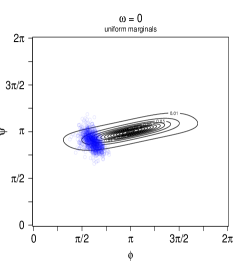
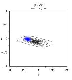
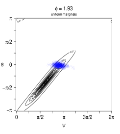
Figure 6: Contour plots of density (5) with uniform marginals, with parameter values estimated by maximum likelihood. The estimates of the copula parameters are $\hat{\rho}_{12}=-0.746,\hat{\rho}_{13}=-0.516,\hat{\rho}_{12}=2.59$.

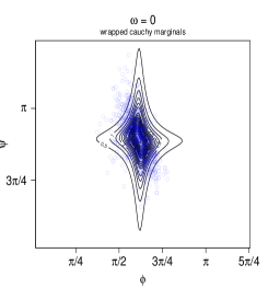
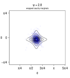
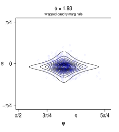
Figure 7: Contour plots of density (5) with wrapped Cauchy marginals, with parameter values estimated by maximum likelihood. The parameters of the marginals are $\hat{\rho}_{1}=0.89,\hat{\mu}_{1}=1.94,\hat{\rho}_{2}=0.86,\hat{\mu}_{2}=2.80,\hat{\rho}_{3}=0.94,\hat{\mu}_{3}=6.22$, where $\hat{\rho}_{i}$ and $\hat{\mu}_{i}$ denote the estimated values for $\rho$ and $\mu$ of density (20) corresponding to the density of the marginal distribution of $\theta_{i}$ for $i\in\{1,2,3\}$, and the copula parameters are $\hat{\rho}_{12}=13,\hat{\rho}_{13}=-0.68,\hat{\rho}_{12}=-0.11$.

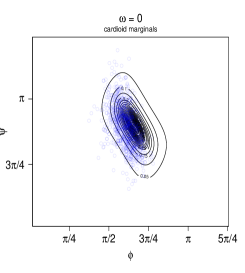
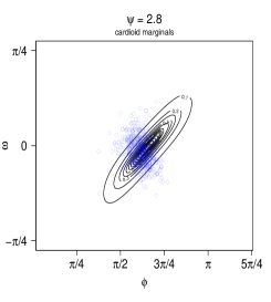
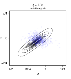
Figure 8: Contour plots of density (5) with cardioid marginals, with parameter values estimated by maximum likelihood. The parameters of the marginals are $\hat{\rho}_{1}=0.5,\hat{\mu}_{1}=1.93,\hat{\rho}_{2}=0.5,\hat{\mu}_{2}=2.81,\hat{\rho}_{3}=0.5,\hat{\mu}_{3}=0$, where $\hat{\rho}_{i}$ and $\hat{\mu}_{i}$ denote the estimated values for $\rho$ and $\mu$ of density $f(\theta;\rho,\mu)=\frac{1}{2\pi}(1+\rho\cos(\theta-\mu))$ corresponding to the density of the marginal distribution of $\theta_{i}$ for $i\in\{1,2,3\}$, and the copula parameters are $\hat{\rho}_{12}=0.59,\hat{\rho}_{13}=1.31,\hat{\rho}_{12}=1.30$.

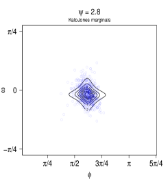
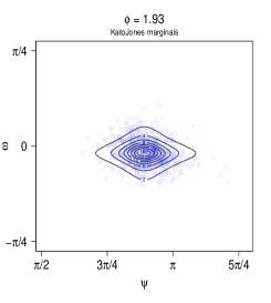
Figure 9: Contour plots of density (5) with Kato–Jones marginals, with parameter values estimated by maximum likelihood. The parameters of the marginals are $\hat{\mu}_{1}=1.93,\hat{\gamma}_{1}=0.94,\hat{\rho}_{1}=0.88,\hat{\lambda}_{1}=0.004,\hat{\mu}_{2}=2.81,\hat{\gamma}_{2}=0.92,\hat{\rho}_{2}=0.85,\hat{\lambda}_{2}=-0.018,\hat{\mu}_{3}=6.23,\hat{\gamma}_{3}=0.97,\hat{\rho}_{1}=0.93,\hat{\lambda}_{1}=-0.004$, where $\hat{\rho}_{i},\hat{\mu}_{i},\hat{\gamma}_{i}$ and $\hat{\lambda}_{i}$ denote the estimated values for $\rho,\mu,\gamma$ and $\lambda$ of the Kato–Jones density as given in [34] corresponding to the density of the marginal distribution of $\theta_{i}$ for $i\in\{1,2,3\}$, and the copula parameters are $\hat{\rho}_{12}=3.24,\hat{\rho}_{13}=1.49,\hat{\rho}_{12}=0.21$.

References

- [1] T. Abe and C. Ley. A tractable, parsimonious and flexible model for cylindrical data, with applications. Econometrics and Statistics, 4:91–104, 2017.
- [2] J. Ameijeiras-Alonso and I. Gijbels. Smoothed circulas: nonparametric estimation of circular cumulative distribution functions and circulas. to appear in Bernoulli, 2024.
- [3] J. Ameijeiras-Alonso and C. Ley. Sine-skewed toroidal distributions and their application in protein bioinformatics. Biostatistics, 23:685–704, 2022.
- [4] Y. Baba. Statistics of angular data: wrapped normal distribution model (in japanese). Proceedings of the Institute of Statistical Mathematics, 28:41–54, 1981.
- [5] W. Boomsma, K. V. Mardia, C. C. Taylor, J. Ferkinghoff-Borg, A. Krogh, and T. Hamelryck. A generative, probabilistic model of local protein structure. Proceedings of the National Academy of Sciences, 105:8932–8937, 2008.
- [6] P. J. A. Cock, T. Antao, J. T. Chang, B. A. Chapman, C. J. Cox, A. Dalke, I. Friedberg, T. Hamelryck, F. Kauff, B. Wilczynski, and M. J. L. de Hoon. Biopython: freely available Python tools for computational molecular biology and bioinformatics. Bioinformatics (Oxford, England), 25(11):1422–1423, 2009.
- [7] C. Czado and I. Van Keilegom. Dependent censoring based on parametric copulas. Biometrika, 110(3):721–738, 2023.
- [8] J. J. Fernández-Durán. Models for circular-linear and circular-circular data constructed from circular distributions based on nonnegative trigonometric sums. Biometrics, 63:579–585, 2007.
- [9] J. J. Fernández-Durán and M. M. Gregorio-Domínguez. Modeling angles in proteins and circular genomes using multivariate angular distributions based on multiple nonnegative trigonometric sums. Statistical Applications in Genetics and Molecular Biology, 13(1):1–18, 2014.
- [10] J. J. Fernández-Durán and M. M. Gregorio-Domínguez. CircNNTSR: An R package for the statistical analysis of circular, multivariate circular, and spherical data using nonnegative trigonometric sums. Journal of Statistical Software, 70(6):1–19, 2016.
- [11] J. J. Fernández-Durán and M. M. Gregorio-Domínguez. Multivariate nonnegative trigonometric sums distributions for high-dimensional multivariate circular data, 2023.
- [12] N. I. Fisher and A. J. Lee. A correlation coefficient for circular data. Biometrika, 70(2):327–332, 1983.
- [13] E. García-Portugués, M. Sörensen, K. V. Mardia, and T. Hamelryck. Langevin diffusions on the torus: estimation and applications. Statistics and Computing, 29:1–22, 2019.
- [14] C. Genest and A.-C. Favre. Everything you always wanted to know about copula modeling but were afraid to ask. Journal of Hydrologic Engineering, 12(4):347–368, 2007.
- [15] C. Genest, K. Ghoudi, and L.-P. Rivest. A semiparametric estimation procedure of dependence parameters in multivariate families of distributions. Biometrika, 82(3):543–552, 1995.
- [16] V. Genna, A. Hospital, and M. Orozco. SARS-CoV-2 Inhibition, Host Selection and Next-Move Prediction Through High-Performance Computing, 2020.
- [17] A. Ghalanos and S. Theussl. Rsolnp: General Non-linear Optimization Using Augmented Lagrange Multiplier Method, 2015. R package version 1.16.
- [18] I. Gradshteyn and I. Ryzhik. Table of Integrals, Series, and Products, 7th ed. Academic Press, San Diego, 2007.
- [19] T. Hamelryck, K. V. Mardia, and J. Ferkinghoff-Borg, editors. Bayesian Methods in Structural Bioinformatics. Springer, Heidelberg, Germany, 2012.
- [20] T. Harder, W. Boomsma, M. Paluszewski, J. Frellsen, K. E. Johansson, and T. Hamelryck. Beyond rotamers: a generative, probabilistic model of side chains in proteins. BMC Bioinformatics, 11:306, 2010.
- [21] A. Jacobsen, E. van Dijk, H. Mouhib, B. Stringer, O. Ivanova, J. Gavaldá-Garciá, L. Hoekstra, K. A. Feenstra, and S. Abeln. Introduction to Protein Structure, 2023.
- [22] S. R. Jammalamadaka, A. Sengupta, and A. Sengupta. Topics in Circular Statistics. World Scientific, 2001.
- [23] H. Joe. Multivariate Models and Multivariate Dependence Concepts. Chapman and Hall/CRC, 1997.
- [24] H. Joe. Dependence Modeling with Copulas. CRC Press, Boca Raton, FL, USA, 2015.
- [25] R. A. Johnson and T. E. Wehrly. Measures and models for angular correlation and angular-linear correlation. Journal of the Royal Statistical Society: Series B (Methodological), 39(2):222–229, 1977.
- [26] R. A. Johnson and T. E. Wehrly. Some angular-linear distributions and related regression models. Journal of the American Statistical Association, 73(363):602–606, 1978.
- [27] G. Jona-Lasinio, A. Gelfand, and M. Jona-Lasinio. Spatial analysis of wave direction data using wrapped Gaussian processes. The Annals of Applied Statistics, 6(4), 2012.
- [28] M. C. Jones and A. Pewsey. A family of symmetric distributions on the circle. Journal of the American Statistical Association, 100(472):1422–1428, 2005.
- [29] M. C. Jones, A. Pewsey, and S. Kato. On a class of circulas: copulas for circular distributions. Annals of the Institute of Statistical Mathematics, 67:843–862, 2015.
- [30] J. Jumper, R. Evans, A. Pritzel, T. Green, M. Figurnov, O. Ronneberger, K. Tunyasuvunakool, R. Bates, A. Žídek, A. Potapenko, A. Bridgland, C. Meyer, S. A. A. Kohl, A. J. Ballard, A. Cowie, B. Romera-Paredes, S. Nikolov, R. Jain, J. Adler, T. Back, S. Petersen, D. Reiman, E. Clancy, M. Zielinski, M. Steinegger, M. Pacholska, T. Berghammer, S. Bodenstein, D. Silver, O. Vinyals, A. W. Senior, K. Kavukcuoglu, P. Kohli, and D. Hassabis. Highly accurate protein structure prediction with AlphaFold. Nature, 596(7873):583–589, 2021.
- [31] P. E. Jupp and K. V. Mardia. A general correlation coefficient for directional data and related regression problems. Biometrika, 67(1):163–173, 1980.
- [32] W. Kabsch and C. Sander. Dictionary of protein secondary structure: Pattern recognition of hydrogen-bonded and geometrical features. Biopolymers, 22(12):2577–2637, 1983.
- [33] S. Kato. A distribution for a pair of unit vectors generated by Brownian motion. Bernoulli, 15:898–921, 2009.
- [34] S. Kato and M. C. Jones. A tractable and interpretable four-parameter family of unimodal distributions on the circle. Biometrika, 102(1):181–190, 2015.
- [35] S. Kato and A. Pewsey. A Möbius transformation-induced distribution on the torus. Biometrika, 102:359–370, 2015.
- [36] S. Kato and K. Shimizu. Dependent models for observations which include angular ones. Journal of Statistical Planning and Inference, 138(11):3538–3549, 2008.
- [37] S. Kim, A. SenGupta, and B. C. Arnold. A multivariate circular distribution with applications to the protein structure prediction problem. Journal of Multivariate Analysis, 143:374–382, 2016.
- [38] F. Lagona. Copula-based segmentation of cylindrical time series. Statistics & Probability Letters, 144:16–22, 2019.
- [39] F. Lagona, M. Picone, and A. Maruotti. A hidden Markov model for the analysis of cylindrical time series. Environmetrics, 26(8):534–544, 2015.
- [40] T. J. Lane. Protein structure prediction has reached the single-structure frontier. Nature Methods, 20(2):170–173, 2023.
- [41] C. Ley, S. Babić, and D. Craens. Flexible models for complex data with applications. Annual Review of Statistics and Its Application, 8:18.1–18.23, 2021.
- [42] C. Ley and T. Verdebout. Modern Directional Statistics. Chapman and Hall/CRC Press, Boca Ratón, Florida, 2017.
- [43] C. Ley and T. Verdebout, editors. Applied Directional Statistics: Modern Methods and Case Studies. Chapman and Hall/CRC Press, Boca Ratón, Florida, 2018.
- [44] B. Li and M. G. Genton. Nonparametric identification of copula structures. Journal of the American Statistical Association, 108(502):666–675, 2013.
- [45] K. Mardia and T. Sutton. A model for cylindrical variables with applications. Journal of the Royal Statistical Society: Series B (Methodological), 40(2):229–233, 1978.
- [46] K. V. Mardia. Statistics of directional data. Journal of the Royal Statistical Society: Series B (Methodological), 37:349–371, 1975.
- [47] K. V. Mardia, G. Hughes, C. C. Taylor, and H. Singh. A multivariate von Mises distribution with applications to bioinformatics. Canadian Journal of Statistics, 36:99–109, 2008.
- [48] K. V. Mardia and P. E. Jupp. Directional Statistics. John Wiley & Sons, Chichester, United Kingdom, 2000.
- [49] K. V. Mardia, J. T. Kent, Z. Zhang, C. C. Taylor, and T. Hamelryck. Mixtures of concentrated multivariate sine distributions with applications to bioinformatics. Journal of Applied Statistics, 2012.
- [50] K. V. Mardia and C. Ley. Directional distributions. In Wiley StatsRef: Statistics Reference Online, pages 1–13. John Wiley & Sons, Ltd, 2018.
- [51] K. V. Mardia, C. C. Taylor, and G. K. Subramaniam. Protein bioinformatics and mixtures of bivariate von Mises distributions for angular data. Biometrics, 63:505–512, 2007.
- [52] G. Mastrantonio. The joint projected normal and skew-normal: A distribution for poly-cylindrical data. Journal of Multivariate Analysis, 165:14–26, 2018.
- [53] P. McCullagh. Möbius transformation and Cauchy parameter estimation. The Annals of Statistics, 24:787–808, 1996.
- [54] A. Navarro, J. Frellsen, and R. Turner. The multivariate generalised von Mises distribution: inference and applications. Proceedings of the Thirty-First AAAI Conference on Artificial Intelligence (AAAI-17), pages 2394–2400, 2017.
- [55] R. B. Nelsen. An Introduction to Copulas. Springer Series in Statistics. Springer, 2nd edition, 2006.
- [56] A. Nodehi, M. Golalizadeh, M. Maadooliat, and C. Agostinelli. Estimation of parameters in multivariate wrapped models for data on a p-torus. Computational Statistics, 36(1):193–215, 2021.
- [57] A. Pewsey and E. García-Portugués. Recent advances in directional statistics (with discussion). TEST, 30(1):1–58, 2021.
- [58] L. Rodriguez-Lujan, C. Bielza, and P. Larrañaga. Regularized multivariate von Mises distribution, 2015. Series Title: Lecture Notes in Computer Science.
- [59] G. S. Shieh and R. A. Johnson. Inference based on a bivariate distribution with von Mises marginals. Annals of the Institute of Statistical Mathematics, 57:789–802, 2005.
- [60] G. S. Shieh, S. Zheng, R. A. Johnson, Y. F. Chang, K. Shimizu, C. C. Wang, and S. L. Tang. Modeling and comparing the organization of circular genomes. Bioinformatics, 27:912–918, 2011.
- [61] H. Singh, V. Hnizdo, and E. Demchuk. Probabilistic model for two dependent circular variables. Biometrika, 89:719–723, 2002.
- [62] M. Sklar. Fonctions de répartition à n dimensions et leurs marges. Annales de l’ISUP, VIII(3):229–231, 1959.
- [63] C. B. Thygesen, C. S. Steenmans, A. S. Al-Sibahi, L. S. Moreta, A. B. Sørensen, and T. Hamelryck. Efficient Generative Modelling of Protein Structure Fragments using a Deep Markov Model. In Proceedings of the 38th International Conference on Machine Learning, pages 10258–10267. PMLR, 2021.
- [64] T. E. Wehrly and R. A. Johnson. Bivariate models for dependence of angular observations and a related Markov process. Biometrika, 66:255–256, 1980.