A HITRAN-formatted UV line list of S2 containing transitions involving $X\,^{3}\Sigma^{-}_{g}$, $B\,^{3}\Sigma^{-}_{u}$, and $B^{\prime\prime}\,{}^{3}\Pi_{u}$ electronic states

Abstract

The sulfur dimer (S2) is an important molecular constituent in cometary atmospheres and volcanic plumes on Jupiter’s moon Io. It is also expected to play an important role in the photochemistry of exoplanets. The UV spectrum of S2 contains transitions between vibronic levels above and below the dissociation limit, giving rise to a distinctive spectral signature. By using spectroscopic information from the literature, and the spectral simulation program PGOPHER, a UV line list of S2 is provided. This line list includes the primary $B\,^{3}\Sigma^{-}_{u}-X\,^{3}\Sigma^{-}_{g}$ ($v^{\prime}$=0-27, $v^{\prime\prime}$=0-10) electronic transition, where vibrational bands with $v^{\prime}$$\geq$10 are predissociated. Intensities have been calculated from existing experimental and theoretical oscillator strengths, and semi-empirical strengths for the predissociated bands of S2 have been derived from comparisons with experimental cross-sections. The S2 line list also includes the $B^{\prime\prime}\,{}^{3}\Pi_{u}-X\,^{3}\Sigma^{-}_{g}$ ($v^{\prime}$=0-19, $v^{\prime\prime}$=0-10) vibronic bands due to the strong interaction with the $B$ state. In summary, we present the new HITRAN-formatted S2 line list and its validation against existing laboratory spectra. The extensive line list covers the spectral range 21 700$-$41 300 cm^-1 ($\sim$242$-$461 nm) and can be used for modeling both absorption and emission.

Introduction

  The sulfur dimer, disulfur (S2), has been observed in ultraviolet (UV) spectra of comets such as IRAS-Araki-Alcock 1983d (A’Hearn et al., 1983) and Hyakutake (Laffont et al., 1998). The impact of comet Shoemaker-Levy 9 with Jupiter produced large amounts of S2 in the stratosphere (Noll et al., 1995) leading to a rich sulfur chemistry (Zahnle et al., 1995). In addition, S2 has been detected in volcanic plumes on Jupiter’s moon Io (Spencer et al., 2000).

S2 is a key intermediary in the exothermic polymerization of elemental sulfur en route to octasulfur, S8 (Kasting et al., 1989; Shingledecker et al., 2020), the stable molecular form. The polymerization of sulfur towards S8 can be interrupted by the photolysis of S2, and it has also been noted that S_nO can photolyze to S_n (Francés-Monerris et al., 2022). Although, formation pathways of polysulfur molecules (including S2) in the atmosphere of Venus are still under debate (Francés-Monerris et al., 2022), it has been suggested that photodissociation of S2 could fill a needed gap in Venusian atmospheric models (Francés-Monerris et al., 2022). While S2 may only be an intermediary observation, its UV absorption can help infer sulfur chemistry even without the detection of S8.

Hobbs et al. (2021) have investigated thermochemical and photochemical sulfur reactions in the atmospheres of warm and hot Jupiters. They found that at 10^-3 bar and at temperatures around 1000 K, mixing ratios of S2 can be up to 10^-5. The recent detection of CO2 (JWST Transiting Exoplanet Community Early Release Science Team et al., 2023), and apparent SO2 absorption feature (Rustamkulov et al., 2022), in the atmosphere of exoplanet WASP-39b has increased the need to better understand the spectroscopy of photochemically produced sulfur species. In particular, for WASP-39b it has been predicted that S2 is a key molecule in the photochemical pathway to forming SO2 and is expected to be the most abundant sulfur-containing molecule at pressures probed by JWST transmission spectra during the evening terminator (Tsai et al., 2022).

While many works have investigated the energy levels and spectrum of S2, including the analysis of perturbations (e.g., Green and Western, 1996) and predissociated bands (e.g., Lewis et al., 2018), an accurate S2 line list that is capable of reproducing the UV spectrum of S2 at high resolution is currently unavailable in the literature or public databases. This was highlighted by Kim et al. (2003) when building their fluorescence model for analyses of cometary spectra. Kim et al. (2003) extended their atlas (Kim, 1994) by including limited experimental information from the literature, which included some direct entries from early experimental works (Ikenoue, 1953, 1960). However, as acknowledged by the authors, their model was still very limited, particularly in terms of accounting for perturbations. Similarly, in analyses of Io spectra, Spencer et al. (2000) used an unpublished line list that was calculated for the purposes of their work. Perturbations were not accounted for and some of the experimental intensity information which now exists was not available at that time (e.g., Stark et al., 2018). Recently, Sarka and Nanbu (2023) have released an ab initio line list of S2, but spin-spitting and perturbation effects have not been accounted for, which limits the accuracy for high resolution applications.

S2 photolysis has previously been estimated in photochemical models based on inferences from solar system cometary analyses (de Almeida and Singh, 1986; Ueno et al., 2009; Hu et al., 2012) and have been scaled by the actinic flux at 300 nm. Use of this approximation can lead to inaccurate photolysis rates on planets orbiting stars of other spectral types (e.g., M-dwarfs), where the shape of the spectral energy distribution (SED) is different than the Sun. Another consequence is that it disregards the photochemical self-shielding, which is caused by overlying S2 and/or other overlying molecules. Hobbs et al. (2021) employed the calculated cross-sections from the Leiden database (Heays et al., 2017), but it should be noted that the photodissociation cross-sections measured subsequently in Stark et al. (2018) differ substantially from those calculated in Heays et al. (2017).

The goal of this work is to provide a reliable publicly available line list of S2. A line-by-line parameterization, such as that employed by the HITRAN database (Gordon et al., 2022), has advantages over available parametrizations for S2 spectra. These line lists are compatible with a majority of community radiative transfer codes, thereby allowing the generation of cross-sections at a variety of thermodynamic conditions and over a wide spectral range. One of the peculiarities of parameterizing the UV line list of the sulfur dimer is that it has to be capable of simulating the UV spectrum at high resolution below the dissociation limit, while also reproducing the diffuse spectrum above the dissociation limit where rovibronic features can not be resolved. Indeed, the predissociation widths of the disulfur transitions that have upper levels above the dissociation limit have widths that reach tens of wavenumber, therefore obscuring the resolved structure of individual transitions. The S2 line list from this work will, therefore, need to be capable of reproducing these effects.

Spectroscopy of the S2 molecule

  S2 is isoelectronic to molecular oxygen, O2. The two molecules have similar electronic states and exhibit similar visible and UV bands. Thus, comparisons between S2 and the much better studied O2 system provide valuable insights when generating a comprehensive S2 line list. Unlike oxygen, S2 is an unstable molecule. In the laboratories it is produced in sulfur-containing flames and discharges since it mainly forms at high temperatures (800 K) (Wheeler et al., 1998). The $B-X$ transition is quite intense and emits a blue color as seen in experimental and cometary spectra.

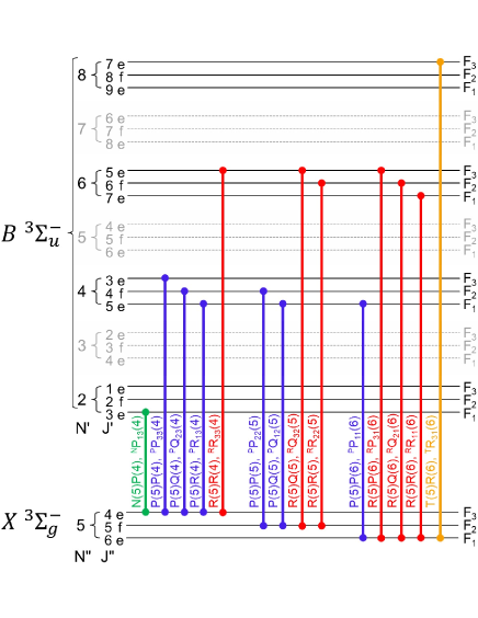
Figure 1: A schematic showing the possible rovibronic transitions for the $B\,^{3}\Sigma^{-}_{u}-X\,^{3}\Sigma^{-}_{g}$ transition of S2 with $N^{\prime\prime}=5$. The ${}^{{\Delta}N}{\Delta}J_{F^{\prime}F^{\prime\prime}}(J^{\prime\prime})$ and $\Delta N$($N^{\prime\prime}$)$\Delta J$($J^{\prime\prime}$) notations are both shown for each transition, with the transition color relating to $\Delta N$. Even $N$ levels of the $X\,^{3}\Sigma^{-}_{g}$ state and odd $N$ levels of the $B\,^{3}\Sigma^{-}_{u}$ (greyed and dashed lines) are not populated. Note that the depicted relative positions of spin components of different rotational levels, are qualitative and do not represent the actual relative energies, especially in the perturbed upper electronic state.

Figure 1 of Sun et al. (2019) provides a detailed comparative overview of the lowest electronic states of S2 and O₂ molecules. Considering that in this work, we concentrate only on the part of the UV spectrum, here, we provide only a brief summary of the states of S2. Just as in the case of molecular oxygen, the ground electronic state of disulfur is $X\,^{3}\Sigma^{-}_{g}$. The lowest excited states are two singlet states $a\,^{1}\Delta_{g}$ and $b\,^{1}\Sigma^{+}_{g}$ with $T_{e}=4322.99$ and 7788.72 cm^-1, respectively (Xing et al., 2013). The electric dipole transitions involving these states and the ground state are spin-forbidden, however, much weaker transitions are possible through magnetic dipole and electric quadrupole mechanisms (Setzer et al., 2003; Fink et al., 1986). Above them lie the $A\,^{3}\Sigma^{+}_{u}$, $A^{\prime}\,{}^{3}\Delta_{u}$, and $c\,^{1}\Sigma^{-}_{u}$ states, which, in the oxygen molecule, are responsible for the so-called Herzberg bands. The electronic state of our interest is $B\,^{3}\Sigma^{-}_{u}$ with term energy $T_{e}=31967.36$ cm^-1, and transition between this state and the ground state are analogous to the so-called Schumann-Runge bands in molecular oxygen. This state is in the close proximity to $B^{\prime}\,{}^{3}\Pi_{g}$ and $B^{\prime\prime}\,{}^{3}\Pi_{u}$ (Xing et al., 2020) states and the interference from the latter has to be taken into account in our line list. At higher energies, near 41 000 cm^-1, lie the $e\,^{1}\Pi_{g}$ and $f\,^{1}\Delta_{u}$ states. S₂ also has a number of unbound electronic states that cross the bound $B\,^{3}\Sigma^{-}_{u}$ state at increasing energy in the order $1\,^{1}\Pi_{u}$, $1\,^{3}\Pi_{g}$, $1\,^{1}\Pi_{g}$, $1\,^{5}\Sigma^{-}_{g}$, $1\,^{5}\Pi_{u}$, and $2\,^{3}\Sigma^{+}_{u}$ (Sun et al., 2019; Wheeler et al., 1998).

In the HITRAN database, the quantum notation of transitions between states obeying Hund’s case (b) is assumed for molecules in triplet states (see Appendix of Gordon et al., 2022). Under this formulation, each rotational level N is split into three spin components with total angular momentum J=N+S, and this notation is adopted here for consistency. In case (b) formalism, the spin components are defined as $F_{1}$: $J=N+1$, $F_{2}$: $J=N$, and $F_{3}$: $J=N-1$. However, as will be seen in the next section, unlike the case of O2, the spin-spin coupling constant of S2 is much larger than the rotational constants causing the splitting of spin components of the individual rotational levels to be larger than the separation between these levels, therefore Hunds case (a) is more appropriate, at least for relatively low rotational levels. Indeed, although S₂ has a $\Sigma$ ground state, the total electron spin is equal to 1, therefore the projection of total angular momentum on the internuclear axis, $\Omega=\Lambda+\Sigma$ (where $\Lambda$ is a projection of orbital angular momentum L, and $\Sigma$ is the projection of total electron spin S), can be 0 or 1. Therefore, S2 can exhibit case (a) behavior. In case (a) formalism of intermediate coupling $F_{1,3}$ are a mixture of $\Omega=0$ and $\Omega=1$ components, whereas $F_{2}$ is pure $\Omega=1$. For the case when the spin components can be considered uncoupled (Hund’s case (c)) $F_{1}$ corresponds to $\Omega=0$ only, whereas $F_{2,3}$ to $\Omega=1$. Just as for the ^16O2 isotopologue in the ground electronic state, in ^32S2 only levels with a total parity (+) are allowed due to nuclear spin statistics (nuclear spin of the ³²S is zero), therefore, in the Hund’s case (b) formalism, every other rotational level (i.e., the even levels) are missing. In the excited $B\,^{3}\Sigma^{-}_{u}$ state, total parity (+) levels will correspond to only even rotational states being populated, and the odd levels are missing.

Selection rules require $\Delta$$J$ to be equal to 0 or $\pm$1 and 14 branches are possible for the $B\,^{3}\Sigma^{-}_{u}-X\,^{3}\Sigma^{-}_{g}$. Traditionally, in spectroscopic papers, the ${}^{{\Delta}N}{\Delta}J_{F^{\prime}F^{\prime\prime}}(J^{\prime\prime})$ notation for line assignments is used. In this notation, it is common to refer to six major branches between the same spin-components (${}^{\textrm{R}}$R₁₁, ${}^{\textrm{R}}$R₂₂, ${}^{\textrm{R}}$R₃₃, ${}^{\textrm{P}}$P₁₁, ${}^{\textrm{P}}$P₂₂, and ${}^{\textrm{P}}$P₃₃) with eight weaker satellite branches (${}^{\textrm{N}}$P₁₃, ${}^{\textrm{R}}$P₃₁, ${}^{\textrm{P}}$Q₁₂, ${}^{\textrm{P}}$Q₂₃, ${}^{\textrm{R}}$Q₃₂, ${}^{\textrm{R}}$Q₂₁, ${}^{\textrm{P}}$R₁₃, and ${}^{\textrm{T}}$R₃₁).

However, in our line list, we employ the $\Delta N$($N^{\prime\prime}$)$\Delta J$($J^{\prime\prime}$) notation, which is closer in appearance to quantum notations given in traditional ASCII files in the static 160-character format in HITRAN. In this notation, seemingly only eight branches are possible for the $B\,^{3}\Sigma^{-}_{u}-X\,^{3}\Sigma^{-}_{g}$ transition: N($N^{\prime\prime}$)P($J^{\prime\prime}$), P($N^{\prime\prime}$)P($J^{\prime\prime}$), P($N^{\prime\prime}$)Q($J^{\prime\prime}$), P($N^{\prime\prime}$)R($J^{\prime\prime}$), R($N^{\prime\prime}$)P($J^{\prime\prime}$), R($N^{\prime\prime}$)Q($J^{\prime\prime}$), R($N^{\prime\prime}$)R($J^{\prime\prime}$), and T($N^{\prime\prime}$)R($J^{\prime\prime}$), where $N^{\prime\prime}$ and $J^{\prime\prime}$ refer to the lower state values. However, both HITRAN and traditional notations are both able to uniquely identify each transition (e.g., T(5)R(6) or ${}^{\textrm{T}}$R₃₁(6) shown in Fig. 1). Although, one has to keep in mind that some of these “branches” in the HITRAN notation represent more than one branch in the traditional notation, for instance, R($N^{\prime\prime}$)R($J^{\prime\prime}$) transitions can be ${}^{\textrm{R}}$R₃₃($J^{\prime\prime}$), ${}^{\textrm{R}}$R₂₂($J^{\prime\prime}$) and ${}^{\textrm{R}}$R₁₁($J^{\prime\prime}$). Nevertheless, since they correspond to the transitions between different spin components, they can be uniquely identified with rotational and total angular momentum quanta in the case (b) framework. Fig. 1 demonstrates all branches of the $B\,^{3}\Sigma^{-}_{u}-X\,^{3}\Sigma^{-}_{g}$ electronic transition with $N^{\prime\prime}=5$ where each individual transition has been labeled with both notations.

In the $B^{\prime\prime}\,{}^{3}\Pi_{u}$ state, $\Omega$ can have values 0, 1, and 2, because $L$=1, also only (+) parity levels are allowed, resulting in every rotational level being populated but missing one of the $\Lambda$-doubling components. For the $B^{\prime\prime}\,{}^{3}\Pi_{u}$–$X\,^{3}\Sigma^{-}_{g}$ transition the following 15 types of branches are possible: N($N^{\prime\prime}$)P($J^{\prime\prime}$), O($N^{\prime\prime}$)P($J^{\prime\prime}$), P($N^{\prime\prime}$)P($J^{\prime\prime}$), Q($N^{\prime\prime}$)P($J^{\prime\prime}$), R($N^{\prime\prime}$)P($J^{\prime\prime}$), O($N^{\prime\prime}$)Q($J^{\prime\prime}$), P($N^{\prime\prime}$)Q($J^{\prime\prime}$), Q($N^{\prime\prime}$)Q($J^{\prime\prime}$), R($N^{\prime\prime}$)Q($J^{\prime\prime}$), S($N^{\prime\prime}$)Q($J^{\prime\prime}$), P($N^{\prime\prime}$)R($J^{\prime\prime}$), Q($N^{\prime\prime}$)R($J^{\prime\prime}$), R($N^{\prime\prime}$)R($J^{\prime\prime}$), S($N^{\prime\prime}$)R($J^{\prime\prime}$), and T($N^{\prime\prime}$)R($J^{\prime\prime}$).

The higher-lying electronic states of S2 are severely perturbed and predissociated. The predissociated bands of S2 are caused by the spin-orbit interaction with the crossing ungerade electronic states (Lewis et al., 2018) and by the $B$ state crossing the dissociation limit after $v$$\geq$10 (Green and Western, 1996). Predissociation causes individual rovibronic lines to have lifetime broadening (FWHM) of up to 50 cm^-1 (Lewis et al., 2018; Wheeler et al., 1998). The lifetime broadening exceeds typical pressure broadening by up to three orders of magnitude and, therefore, results in a series of unresolved bands at higher frequencies. Although well described by the Lorentzian profile (as both pressure and predissociation line-widths are lifetime-driven broadening), the predissociation widths do not have the pressure and temperature dependence unlike pressure-broadened widths.

The ungerade electronic states are responsible for contributing to the predissociation. Patiño and Barrow (1982) proposed that the primary perturber of the lower vibrational levels of the $B$ state was the $B^{\prime\prime}\,{{}^{3}}\Pi_{u}$ state. Matsumi et al. (1984, 1985) were able to measure the transitions involving $B^{\prime\prime}\,{{}^{3}}\Pi_{u}$ state directly, and Figure 2 of Matsumi et al. (1985) effectively shows the nature of perturbations. For higher vibronic levels, Wheeler et al. (1998) have predicted that the ${}^{1}\Pi_{u}$ state was the primary culprit for predissociating the $v^{\prime}$$\leq$16 bands and also suggested that the 1${}^{5}\Pi_{u}$ state is responsible for predissociating the $v^{\prime}$$\geq$17 bands. Lewis et al. (2018) also do not expect the $B^{\prime\prime}$ state to be the primary source of the significant predissociation for the bands $v^{\prime}=11$-16. Instead, they support that theory of Wheeler et al. (1998) that the primary perturbers are the ${}^{1}\Pi_{u}$ and 1$\,{}^{5}\Pi_{u}$ states (for the bands $v^{\prime}$$\geq$12 and $v^{\prime}$$\geq$17 respectively), along with 2$\,{}^{3}\Sigma^{+}_{u}$ state for the bands $v^{\prime}$$\geq$23.

There is a century-long history of experimental works that have analyzed the UV spectrum of S2 (Naudé and Christy, 1931; Olsson, 1936; Ikenoue, 1953; Meakin and Barrow, 1962; Heaven et al., 1984; Matsumi et al., 1984, 1985; Green and Western, 1996, 1997; Lewis et al., 2018). Large perturbations, which cause the regular patterns within branches to break, are a consequence of the $B^{\prime\prime}$ state. Historically, these perturbations had made high-resolution analyses difficult, but Green and Western (1996) and Green and Western (1997) were able to provide a deperturbed rotational analysis for the $B-X$ and $B^{\prime\prime}-X$ transitions that could accurately model laser-induced fluorescence spectra. Wheeler et al. (1998) have investigated the predissociated bands of the $B-X$ transition as well as the perturbing levels. More recently, cross-sections of S2 have been measured at 370 K and 823 K using a synchrotron facility by Stark et al. (2018). These spectra were analyzed by Lewis et al. (2018) to develop a model for the UV spectrum of S2 that includes the $B-X$ predissociated bands.

In each of these prior works, rotational constants, and model details have been provided, with some earlier works providing measured line positions. However, a line list that can be used directly in radiative transfer models was not available. Recently, an ab initio line list has become available (Sarka and Nanbu, 2023) that can be used to simulate the spectrum of S2. Spin-splittings and perturbation constants were not included, which has a number of limitations when used for high-resolution applications.

Figure 2: S2 potential energy curves for the $X$, $B$ and $B^{\prime\prime}$ states. The vibrational levels of the $X$ and $B$ states used in this work have been included, along with the dissociation limit. Shaded areas demonstrate the strongest transitions according to the Franck-Condon principle for absorption (shaded blue) and emission (shaded red) between the $X$ and $B$ states. The potential energy curves have been plotted using data from Xing et al. (2020). The dissociation limit of 35 636.9 cm^-1 (Sun et al., 2019) is indicated, demonstrating it proximity to the $v^{\prime}=10$ level of the $B$ state.

Fig. 2 provides a schematic of the potential energy curves (PEC) of the $X$, $B$, and $B^{\prime\prime}$ states (Xing et al., 2020). Due to the Franck-Condon principle; respective positions of the PECs; and the fact that in excited vibrational states, the overlap integrals are most efficient near the walls of the potentials, the absorption from the ground state ($v^{\prime\prime}=0$) would be most efficient to the higher vibrational states of the excited state (blue shaded region). Due to the same logic, the emission from the $v^{\prime}=0$ of the $B^{\prime\prime}$ state will be most efficient to the excited vibrational levels of the ground electronic state (red-shaded region).

The PGOPHER S2 model

 

The S2 line list for this work has been built using the PGOPHER program (Western, 2017), which applies spectroscopic constants to calculate transition frequencies and intensities. Our S2 model is, in large part, constructed from the analysis by Green and Western (1996) and Green and Western (1997) for rovibrational bands below the dissociation limit. In these works, laser-induced fluorescence spectra containing $B-X$ transitions of S2 were fit to a Hamiltonian that simultaneously accounted for perturbations caused by the interacting $B^{\prime\prime}$ state. In our work, some of these constants have been refit using observed emission lines of S2 (Olsson, 1936; Ikenoue, 1960; Patiño and Barrow, 1982). There are also later experimental works that reported measurements of rovibronic lines of S₂ (Heaven et al., 1984; Matsumi et al., 1984, 1985). However, they report only spectroscopic constants and not the actual line positions. Considering severe perturbations, it is impossible to recreate line positions from these constants without having the original program. Moreover, even with these details, these constants may not work. Anecdotally, Matsumi et al. (1984) have acknowledged that the constants provided in Table I of their paper are tentative and do not reproduce the observed line positions even at lower rotational quanta. In order to build global spectroscopic models, is imperative (Gordon et al., 2016) that the experimental papers provide original measured line positions along with fitted constants.

Table 1 provides the term values ($T_{v}$), rotational constants ($B$), spin-spin coupling ($\lambda$), spin-rotation coupling ($\gamma$), centrifugal distortion ($D$), and the centrifugal distortion of spin-spin coupling ($\lambda_{D}$) for $v^{\prime\prime}=0$-10 of the $X\,^{3}\Sigma^{-}_{g}$ state of ^32S_2 used in this work. Constants from Green and Western (1996) were used for the $v^{\prime\prime}=0$, 1, 5 levels and PGOPHER was used to refit constants for other levels using selected line positions of the $B-X$ ($v^{\prime}$,$v^{\prime\prime}$) = (2,2), (3,2), (1,3), (2,3), (3,3), (1,4), (2,4) (Olsson, 1936), (1,4) (Patiño and Barrow, 1982), and (0,7), (0,8), (0,9), (0,10) (Ikenoue, 1960) emission bands. The $v^{\prime\prime}=6$ level was not part of the Green and Western (1996) model, however, due to the expected importance for S2 emission in cometary spectra, we have included the $v^{\prime\prime}=6$ level by calculating $T_{6}=\omega_{e}(6.5)-\omega_{e}x_{e}(6.5)^{2}-T_{0}=4234.45$ cm^-1 and $B_{v=6}=B_{e}-\alpha(6.5)+\gamma(6.5)^{2}=0.2851$ cm^-1 using constants provided by Huber and Herzberg (1979). Barrow and Yee (1974) also provide parameters to calculate $\lambda_{v=6}=12.246$ cm^-1 and $\gamma_{v=6}=-7.409\times 10^{-3}$ cm^-1. These have been added to our PGOPHER model to complete the $X\,^{3}\Sigma^{-}_{g}$ state for $v^{\prime\prime}=0$-10.

Table 1: Deperturbed spectroscopic parameters used in the PGOPHER model for $v^{\prime\prime}=0$-10 vibrational levels of the $X\,^{3}\Sigma^{-}_{g}$ state. All values are provided in wavenumber (cm^-1) and have been refit using line positions in Olsson (1936), Ikenoue (1960), and Patiño and Barrow (1982). Those values unchanged from Green and Western (1996) have been indicated.

$v^{\prime\prime}$	$T_{v^{\prime\prime}}$	$B$	$\lambda$	$\gamma$ ($10^{-3}$)	$D$ ($10^{-7}$)	$\lambda_{D}$ ($10^{-5}$)
0	0.0a	0.2945923a	11.7931a	-7.157a	1.96a	1.05a
1	719.995a	0.2929975a	11.8659a	-7.148a	1.97a	1.05a
2	1433.930	0.2915728	11.9707	-7.725	2.33	$-$
3	2142.521	0.2899329	12.0575	-7.138	2.15	$-$
4	2845.305	0.2883575	12.1225	-8.280	2.08	$-$
5	3542.94a	0.2844a	12.163a	-7.283a	2.12a	$-$
6	4234.45b	0.2851b	12.246b	-7.409b	1.90b	$-$
7	4920.288	0.2827382	12.2883	-34.412	-0.359	$-$
8	5600.123	0.2815478	12.3233	-33.118	1.02	$-$
9	6274.896	0.2798292	12.3240	-43.742	-0.0151	$-$
10	6943.861	0.2779413	12.3744	-50.146	-1.38	$-$
a From Green and Western (1996).
b Calculated from Huber and Herzberg (1979) and Barrow and Yee (1974), see text for details.

The $B\,^{3}\Sigma^{-}_{u}$ state for ^32S_2 in our model includes vibrational levels from below and above the dissociation limit. Deperturbed constants ($T_{v}$, $B$, $\lambda$, $\gamma$, $D$, $\lambda_{D}$) for the $v^{\prime}=0$-10 levels of the $B$ state have been added to our model using the values available in Green and Western (1996) and Green and Western (1997). These levels mainly lie below the dissociation limit and can be resolved in experimental spectra. Table 2 summarizes constants for the $v^{\prime}=0$-3 levels that were refit using PGOPHER simultaneously with those in the $X$ state using line positions from Olsson (1936), Ikenoue (1960) and Patiño and Barrow (1982). It should be noted that Green and Western (1997) only recommend the $v^{\prime}=7$-9 constants for modeling the lower rotational levels, while the $v^{\prime}=10$ constants are approximate because of difficulty modeling this rovibronic transition – a consequence of its close proximity to the dissociation limit.

Table 2: Deperturbed spectroscopic parameters used in the PGOPHER model for $v^{\prime}=0$-3 vibrational levels of the $B\,^{3}\Sigma^{-}_{u}$ state. All values are provided in wavenumber (cm^-1) and have been refit to line positions in Olsson (1936), Ikenoue (1960), and Patiño and Barrow (1982).

$v^{\prime}$	$T_{v^{\prime}}$	$B$	$\lambda$	$\gamma$ ($10^{-3}$)	$D$ ($10^{-7}$)
0	31672.413	0.223631	4.1813	123.425	16.20
1	32102.782	0.223070	4.8517	-23.489	2.48
2	32525.293	0.223487	2.8111	-8.854	6.89
3	32943.385	0.219805	3.8772	0.173	2.93

Accurate modeling of the $B-X$ transition requires consideration of the interacting $B^{\prime\prime}\,{}^{3}\Pi_{u}$ state of ^32S_2. In our model, deperturbed constants ($T_{v}$, $B$, $D$, $\lambda$, $\gamma$, the spin-orbit coupling $A$, and the $\Omega=0$ lambda doubling constant $o$) are included for the $B^{\prime\prime}$ $v^{\prime}=0$-11 (Green and Western, 1996) and $B^{\prime\prime}$ $v^{\prime}=12$-21 (Green and Western, 1997) levels.

As discussed above, the $B^{\prime\prime}-B$ perturbation is essential to provide accurate positions for lines within each interacting band. The Hamiltonian model of Green and Western (1996) accounts for perturbations of vibronic levels through interacting spin-orbit ($\alpha$) and $L$-uncoupling parameters ($\beta$), along with the corresponding centrifugal distortion parameters ($\alpha_{D}$, $\beta_{D}$). PGOPHER allows the inclusion of the $B^{\prime\prime}-B$ interaction parameters from Green and Western (1996) and Green and Western (1997), but a difference in definition requires $\alpha$ and $\alpha_{D}$ from these work to be multiplied by $-3\sqrt{2}$. In conjunction with the PGOPHER fitting for the $X$ and $B$ states indicated above, the perturbation constants for the interacting $B^{\prime\prime}v^{\prime}-Bv^{\prime}=2$-0, 3-1, 4-1, 4-2, 5-2 states were also refitted using line positions from Olsson (1936), Ikenoue (1960) and Patiño and Barrow (1982) and are given in Table 3. All other perturbation constants were provided by Green and Western (1996) and Green and Western (1997). Overall, perturbation parameters in our model span vibrational levels $v^{\prime}=0$-9 for the $B$ state, and $v^{\prime}=0$-19 for the $B^{\prime\prime}$ state. As noted earlier, the difficulty in the analysis of the $B$ $v^{\prime}=10$ level means that perturbation constants are unavailable.

Table 3: Perturbation constants (in cm^-1) that have been refit using line positions available from Olsson (1936), Ikenoue (1960), and Patiño and Barrow (1982).

$B^{\prime\prime}v^{\prime}-Bv^{\prime}$	$\alpha$	$\alpha_{D}$ ($10^{-3}$)	$\beta$ ($10^{-2}$)	$\beta_{D}$ ($10^{-5}$)
$2-0$	-50.3926	4.3987	29.9227	-12.0297
$3-1$	-61.8478	1.1998	-7.9430	$-$
$4-1$	39.1613	1.8540	3.1993	$-$
$4-2$	$-$	7.7830	-5.3971	-2.8794
$5-2$	50.5328	2.8417	7.2030	$-$

Considering those bands above the dissociation limit, Lewis et al. (2018) have built a coupled-channel model of the $B-X$ transition to account for predissociation of the $v^{\prime}=11$-27 vibrational levels of the $B$ state. Term energies in Lewis et al. (2018) are provided with respect to the $F_{2}$, $v=J=0$ level of the $X\,^{3}\Sigma^{-}_{g}$ state and are separated for each $\Omega$ component (i.e., Hunds case (c) coupling was assumed). As we discussed above, this level does not actually exist for the principle isotopologue due to nuclear spin statistics, and in our PGOPHER model, this virtual state would be at an energy of 8.2 cm^-1. To implement the term values of Lewis et al. (2018) into our PGOPHER model, a calibration is required that removes the artificially applied splitting and accounts for the energy of the $F_{2}$, $v=J=0$ level of the $X\,^{3}\Sigma^{-}_{g}$ state. This essentially adds $\lambda+8.2$ cm^-1 to each $\Omega=0$ term value of Lewis et al. (2018). Our calibrated term values are provided in Table 4, along with rotational constants and predissociation widths determined from Lewis et al. (2018). For some bands, we have slightly adjusted the rotational constants for better agreement at higher temperatures, as indicated in Table 4. Lewis et al. (2018) also recommend $\gamma=0.02$ cm^-1 for all vibrational levels of the $B$ state and this value is also included in our model for the $v^{\prime}=11$-27 vibrational levels of the $B$ state.

Table 4: Spectroscopic parameters used in the PGOPHER model for $v^{\prime}=11$-27 vibrational levels of the $B\,^{3}\Sigma^{-}_{u}$ state. All values are provided in cm^-1 and those values that have been adjusted from Lewis et al. (2018) have been indicated.

$v^{\prime}$	$T_{v^{\prime}}$a	$B$b	$\lambda$b	$\Gamma_{\textrm{HWHM}}$c
11	36 108.4	0.2050	3.0	5.05
12	36 475.8	0.2028	0.5	6.35
13	36 841.1	0.2030d	1.7	7.85
14	37 200.1	0.2005	3.3	5.75
15	37 551.4	0.1970d	3.4	4.15
16	37 895.8	0.1945d	2.5	3.30
17	38 232.3	0.1920d	1.7	3.45
18	38 560.1	0.1909	1.3	8.80
19	38 889.0	0.1921	2.8	25.05
20	39 233.8	0.1908	5.0	24.85
21	39 539.6	0.1796	5.3	3.20
22	39 850.1	0.1876	3.6	17.35
23	40 143.7	0.1765	4.9	5.25
24	40 445.1	0.1793	4.6	9.45
25	40 721.7	0.1782	3.2	14.45
26	40 998.2	0.1696	4.3	3.15
27	41 277.1	0.1718	7.9	6.20
a Term values have been calibrated from the separated $\Omega$ components in Lewis et al. (2018). See text for details.
b Calculated values from Lewis et al. (2018), unless otherwise stated.
c Based on the average calculated values in Lewis et al. (2018).
d Constant has been refit for this work.

Refitting rotational constants for emission bands

 

Green and Western (1996) provided a deperturbed analysis of the $B-X$ transition of S2 with $v^{\prime}=0$-6, $v^{\prime\prime}=0$-7, and the inclusion of perturbations from $v^{\prime}=2$-12 of the $B^{\prime\prime}$ state . Their work used a combination of line positions observed from laser-induced fluorescence spectra (primarily from lower $J$ levels) and previously recorded high-temperature static cell measurements (including levels with $J$ up to 100). In total, 3320 observed lines went into the fitting of their initial S2 model.

Applying the rotational constants of Green and Western (1996) into an initial model for this work, comparisons were made to the measured positions for the $B-X$ ($v^{\prime}$,$v^{\prime\prime}$) = (2,2), (3,2), (1,3), (2,3), (3,3), (1,4), (2,4) bands from Olsson (1936), the (1,4) band from Patiño and Barrow (1982), and the (0,7) band from (Ikenoue, 1960). Mismatched assignments due to band crossings were removed, however there remained differences of up to $~{}2$ cm^-1 to the remaining 864 observed line positions. Overlaying the output of our initial model to the fluorescence spectrum of the (3,3) band recorded by Heaven et al. (1984) implied that the lower $J$ levels were in good agreement. Therefore, to better match the observations of Olsson (1936); Patiño and Barrow (1982); Ikenoue (1960) some modeled lines were included in the refitting of the rotational constants from Green and Western (1996) to restrain the fitted parameters. The first five lines of the ${}^{\textrm{R}}$R₁₁($J^{\prime\prime}$), ${}^{\textrm{R}}$R₂₂($J^{\prime\prime}$), ${}^{\textrm{R}}$R₃₃($J^{\prime\prime}$), ${}^{\textrm{P}}$P₁₁($J^{\prime\prime}$), ${}^{\textrm{P}}$P₂₂($J^{\prime\prime}$), and ${}^{\textrm{P}}$P₃₃($J^{\prime\prime}$) branches of the (2,2), (3,2), (1,3), (2,3), (3,3), (1,4), (2,4), and (0,7) bands were included in the fit using the line positions of our initial model (i.e., predicted using constants from Green and Western, 1996). This effectively limited the impact of the refitting for the lower $J$ levels of these bands, while giving enough flexibility of the fit to account for the measurements of Olsson (1936); Patiño and Barrow (1982); Ikenoue (1960). It was also necessary to fit the perturbation constants as they have a significant influence on the resultant spectrum. The refitting of the constants for these bands yielded a standard deviation of 0.133 cm^-1.

Ikenoue (1960) also included measured positions for the (0,8), (0,9), and (0,10) bands. This allowed the rotational constants of the $v^{\prime\prime}=8$, 9, and 10 levels to be predicted, which were not available in Green and Western (1996). These bands were fit using 266 line position from Ikenoue (1960) to give a standard deviation of 0.116 cm^-1.

In total, 1378 lines were used for a standard deviation of 0.130 cm^-1. The constants for levels of the $B-X$ transition that were fit for this work are provided in Tables 1, 2, and 3.

Determining band strengths for predissociated region

 

Theoretical oscillator strengths ($f_{v^{\prime}v^{\prime\prime}}$) are reported in the literature for many bands of ^32S_2 (Pradhan and Partridge, 1996; Smith and Liszt, 1971). However, these works do not cover all of the $B-X$ predissociated bands measured by Stark et al. (2018) and often do not include hot bands. The Einstein-A coefficients reported by Xing et al. (2020) have been converted to oscillator strengths using the formulae in Bernath (2016). In addition, some works (Anderson et al., 1979; da Silva and Ballester, 2019; Xing et al., 2020) report the Frank-Condon (FC) factors ($q_{v^{\prime}v^{\prime\prime}}$), but these have not been implemented in this work.

Figure 3: Oscillator strengths ($f_{v^{\prime},0}$) factors for the bands of the $B-X$ transition of ^32S_2, plotted against $v^{\prime}$ with $v^{\prime\prime}=0$ (Smith and Liszt, 1971; Stark et al., 2018; Pradhan and Partridge, 1996; Xing et al., 2020). Also included are oscillator strengths from this work that were obtained by fitting to experimental absorption cross sections at 370 and 823 K from Stark et al. (2018).

Fig. 3 provides a comparison of the oscillator strengths considered in this work for $B-X$ bands with $v^{\prime\prime}=0$. Generally, there is a good agreement between Stark et al. (2018) and Xing et al. (2020) for fundamental bands with $v^{\prime}<10$. However, since the the oscillator strengths of Pradhan and Partridge (1996) and Smith and Liszt (1971) do not align well with those of Stark et al. (2018), it was necessary to fit the oscillator strengths using PGOPHER (Western, 2017) for the $v^{\prime}\geq 10$ fundamental bands using the calibrated cross-sections at 370 and 823 K (Stark et al., 2018).

PGOPHER requires the square root of the band strength (i.e, $\sqrt{S}$) in order to scale the strength of the corresponding transition and individual line intensities. These can be converted to oscillator strengths using the formulae in Bernath (2016). The resultant oscillator strengths determined from the fit are shown in Fig. 3 and provided in Table 5. The fitted values appear consistent with those from Stark et al. (2018) and Xing et al. (2020) for the $v^{\prime}<10$ bands and also are in qualitative agreement when compared to the oscillator strengths for the predissociated region presented in Figure 6 of Stark et al. (2018). Our fit also indicates that the band with the strongest overlap (i.e., maximum oscillator strength) appears at $v^{\prime}=12$, which is a slightly lower vibrational level than that of Pradhan and Partridge (1996) and Smith and Liszt (1971), but consistent with the vibrational level reported by Stark et al. (2018).

Hot bands with $v^{\prime\prime}=1$ are also prominent in the Stark et al. (2018) spectra, particularly at 823 K, therefore it was also necessary to fit the oscillator strengths for $v^{\prime}\geq 13$ for these bands. The fitted oscillator strengths for the hot bands are also given in Table 5.

For $B-X$ bands with $v^{\prime\prime}=0$ below the dissociation limit ($v^{\prime}$=0-9), the oscillator strengths calculated from Xing et al. (2020) have been used, given the consistency with Stark et al. (2018) for the $v^{\prime\prime}=0$ bands. Oscillator strengths calculated from Xing et al. (2020) were also used for the $v^{\prime\prime}=1$ and $v^{\prime\prime}=2$ hot bands up to $v^{\prime}$=10. The oscillator strengths for the $v^{\prime}=11$-12 bands have been estimated due to the lack of consistency between literature values. Oscillator strengths for the $v^{\prime\prime}=2$ hot bands with $v^{\prime}$=11-20 are provided by Pradhan and Partridge (1996), with an estimated strength for the $v^{\prime}$=21-27 bands.

A summary of the oscillator strengths used in this work for the $B-X$ bands with $v^{\prime\prime}=0$-2 is provided in Table 5. For $B-X$ bands with $v^{\prime}=0$-3 and $v^{\prime\prime}=3$-10, oscillator strengths calculated from Xing et al. (2020) have been used.

Table 5: Oscillator strengths ($f_{v^{\prime},v^{\prime\prime}}$) used in this work for ^32S_2. These include those obtained from fits to experimental cross-sections at 370 and 823 K (Stark et al., 2018), and when indicated, those taken from the literature.

$v^{\prime}$	$f_{v^{\prime},0}$ ($10^{2}$)	$f_{v^{\prime},1}$ ($10^{2}$)	$f_{v^{\prime},2}$ ($10^{2}$)
0	0.00028a	0.00322a	0.01818a
1	0.00231a	0.02202a	0.09851a
2	0.00993a	0.07709a	0.26882a
3	0.02971a	0.18455a	0.48764a
4	0.06932a	0.33894a	0.65007a
5	0.13428a	0.50620a	0.66086a
6	0.22537a	0.63762a	0.51167a
7	0.33722a	0.69030a	0.28159a
8	0.45872a	0.64932a	0.08544a
9	0.57501a	0.52711a	0.00129a
10	0.82326	0.36166a	0.04160a
11	0.95497	0.18455b	0.00300c
12	1.04341	0.07709b	0.01200c
13	1.01371	0.27715	0.06200c
14	0.95778	0.35418	0.12800c
15	0.87753	0.40679	0.19200c
16	0.78794	0.50050	0.23800c
17	0.65796	0.58404	0.26200c
18	0.57876	0.81386	0.26200c
19	0.57341	0.94788	0.24200c
20	0.44291	0.75558	0.21000c
21	0.32794	0.52221	0.19053b
22	0.29978	0.69719	0.17074b
23	0.21819	0.61324	0.15054b
24	0.19473	0.55452	0.13004b
25	0.18400	0.57918	0.10913b
26	0.14052	0.48191	0.08792b
27	0.13119	0.48519	0.06641b
a Calculated from Xing et al. (2020).
b Estimated values.
c Pradhan and Partridge (1996).

S2 line list for HITRAN

  The line list generated for ^32S_2 from PGOPHER has been converted into the standard format used by the HITRAN database (Gordon et al., 2022). This format is used as input to numerous radiative transfer codes for terrestrial and exoplanetary applications, and is expected to be included into the HITRAN database (for this work, 58 is used as a provisional molecule ID number). Line positions (in cm^-1), intensities (cm/molecule at 296 K), Einstein-$A$ values (s^-1), lower-state energies (cm^-1), and transition assignments have been converted directly from PGOPHER. It is necessary to include pressure broadening parameters for each line so that spectra can be calculated from the line list. For this work, air- and self-broadening Voigt parameters have been estimated as 0.05 cm^-1/atm for both. In addition, the temperature dependence of the broadening has been estimated as 0.71. These values have been approximated based on comparisons to similar parameters in HITRAN for O₂. The line intensities in HITRAN formalism are scaled due to the “natural” terrestrial abundance of atomic species taken from De Biévre et al. (1984). Therefore, the intensities in PGOPHER for 100% ^32S_2 are scaled by 0.9028 in the HITRAN-formatted line list.

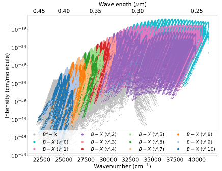
Figure 4: An overview of the S2 line list calculated for this work. Vibronic bands of the $B-X$ transition (with $v^{\prime}$=0-27, $v^{\prime\prime}$=0-10) are indicated. The line positions (cm^-1) have been plotted against intensity (cm/molecule at 296 K) scaled by their natural abundance for ^32S_2.

An overview of the S2 line list has been provided in Fig. 4. The line list includes $B-X$ bands up to $v^{\prime}=27$ and spans the 21 700$-$41 300 cm^-1 ($\sim$242$-$461 nm) spectral range. The vertical axis shows intensity in HITRAN units and formalism (at 296 K), which assumes local thermal equilibrium. That is why the bands with high $v^{\prime\prime}$ values appear so weak, as these levels will have a very small population at 296 K. However, as shown in Figure 2, one should expect strong emissions down to these levels from photochemically excited lower levels of the excited electronic state.

In addition to the line list, a partition sum, $Q$, is also required to recalculate line intensities at different temperatures. For this work, the total internal partition sums ($Q_{\textrm{sum}}$) for ^32S2 has been exported from the PGOPHER model, which employs direct summation of the energy levels. For consistency with other molecules in HITRAN, the $Q_{\textrm{sum}}$ values have been placed on the same temperature grid used in TIPS-2021 (Gamache et al., 2021). In addition, the lower state energies have been adjusted to the energy of the lowest occupied level (i.e., +15.120664 cm^-1 has been added to all energies) to be consistent with HITRAN format, and the partition sum exported from PGOPHER. The S2 HITRAN metadata and partition sum can be seamlessly implemented into the HITRAN Application Programming Interface, HAPI (Kochanov et al., 2016), to enable the calculation of cross sections for this work. The HITRAN-formatted S2 line list is provided as a supplementary file, along with the partition sum to allow calculation with HAPI.

As noted earlier, the S2 diffuse $B-X$ bands in the UV require the inclusion of predissociated line widths in order to generate reliable cross-sections. Lewis et al. (2018) provides separate calculated predissociation widths for each $\Omega$ for the $v^{\prime}$$\geq$10 $B-X$ bands. These have been averaged for each vibrational level and are provided as half width at half maximum (HWHM) values in Table 4. A Python code has been generated to be used alongside HAPI in order to calculate absorption cross-sections with the inclusion of predissociated line widths. This code is provided as a Supplementary file and is expected to be incorporated into future versions of HAPI. It is anticipated that it will also be of benefit to the calculation of predissociation for other molecules in HITRAN, in particular for the Schumann-Runge bands of O2.

Results

 

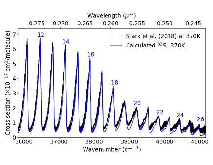
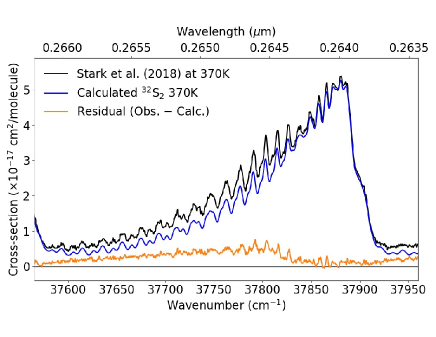
Figure 5: Experimental S2 absorption cross section at 370 K from Stark et al. (2018) compared to a calculated spectrum (blue) that uses the line list from this study. The upper panel shows an overview of the predissociated region between 35 400-41 500 cm^-1 with even $v^{\prime}$ indicated for the $B-X$ ($v^{\prime}$,0) bands. The lower panel shows a zoomed-in region around the $B-X$ (16,0) band as it has the smallest predissociated width, with a residual (Obs.-Calc.) shown in orange. Predissociated bands with $v^{\prime}$$\geq$10 have been calculated using the Lorentz HWHM values given in Table 4.

The line list generated in this work has been validated by comparing calculated spectra to the measurements of Stark et al. (2018) at 370 and 823 K, as was done by Lewis et al. (2018). All spectra in this work have been calculated using HAPI with the inclusion of the presdissociation widths. The upper panel of Fig. 5 shows the S2 line list calculated at 370 K and plotted against the calibrated cross-section from Stark et al. (2018). The lower panel of Fig. 5 shows a zoomed-in region of the upper panel around the $v^{\prime}=16$ band of the $B-X$ transition with the residual (Obs.-Calc.) also shown. The $B-X$ bands above the dissociation limit exhibit a similar structure, but the size of the predissociation widths can obscure much of the detail. Spin-spin splitting leads to a separation of each $\Omega$ component and, depending on the magnitude of the separation and predissociation widths, the $\Omega=0$ branches can be seen as a shoulder to the bandhead as shown for the $v^{\prime}=16$ band near 37 900 cm^-1. In addition, the predissociation widths for this level are small enough to resolve partial rotational structure, which agrees very well with the measurements of Stark et al. (2018). Some of the calculated intensity in this band is due to the underlying hot bands.

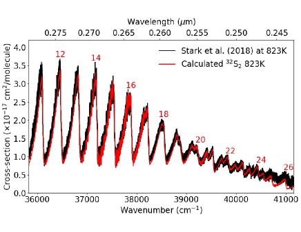
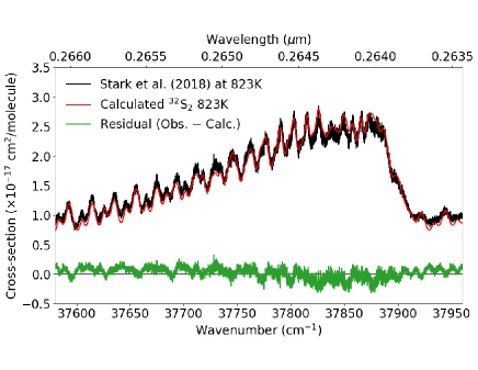
Figure 6: Experimental S2 absorption cross section at 823 K from Stark et al. (2018) compared to a calculated spectrum (red) using line list from this work. The upper panel shows an overview of predissociated region between 35 400-41 500 cm^-1, with even $v^{\prime}$ indicated for the $B-X$ ($v^{\prime}$,0) bands. Hot bands have not been indicated, but are prominent in between the ($v^{\prime}$,0) sequence. The lower panel shows a zoomed-in region around the (16,0) band. This band has the smallest predissociated width, which partially reveals the rotational structure. The residual (Obs.-Calc.) is shown in green.

For this work, hot bands to the $v^{\prime\prime}=1$ and $v^{\prime\prime}=2$ of the $X$ state have been included. These bands become more dominant at higher temperatures, and Figure 6 shows comparisons to the 823 K cross section of Stark et al. (2018). The oscillator strengths for our model have been determined by comparing the intensities at both 370 and 823 K. At this higher temperature, good agreement is also seen with the spectrum calculated using the line list from this work.

Discussion

  The primary challenge in this work was to combine the constants and parameters of previous works into a consistent model that can be used for calculating the spectrum of S₂ in the UV. Since the spectral range of the $B-X$ line list spans the dissociation limit of S₂, there is a different classification of the accuracy of individual spectroscopic parameters above and below this limit. Below the dissociation limit for bands with $v^{\prime}\leq 9$, the perturbation model substantially improves the accuracy of the line positions, as demonstrated by the refitting of the rotational constants. However, for bands above the dissociation limit with $v^{\prime}\geq 11$, the position accuracy is difficult to estimate as the lines are broadened due to predissociation, and perturbations for these bands are not included. It should be expected that these bands are consistent with those of Lewis et al. (2018), and have a conservatively estimated position accuracy of $\sim$10 cm^-1.

For bands involving levels below predissociation, a standard deviation of all fitted lines is 0.130 cm^-1, which is much higher than above the predissociaion. Figure 7 includes a comparison of the line list and calculated cross section from this work (at 300 K) to the measurements of Green and Western (1996) in the region of the $B-X$ (5,0) transition. While the intensity of the experiment is not equivalent to the absorption cross section, the agreement of the line positions is excellent and demonstrates the accuracy of these bands. Strong perturbations of the $B-X$ (5,0) band with the $B^{\prime\prime}-X$ (10,0) have a significant impact on the line positions. Moreover, the $\Omega$ splitting also impacts the line positions and significantly alters the location of each band head. Including these effects is essential for reproducing experimental observations as demonstrated in Figure 7 for the comparison to the absorption cross section from ab initio work of Sarka and Nanbu (2023), which does not account for spin-splitting or perturbations. Furthermore, the predissociation widths included in Sarka and Nanbu (2023) does not agree with the predissociation broadening observed in the experiments of Stark et al. (2018).

It should be highlighted that only a limited number of line positions could be used when refitting the constants. Rotational constants have primarily been provided by previous works, which allows for a model to be constructed that works reasonably well for unperturbed levels. However, for a molecule like S2 where large interactions substantially perturb the levels and observed line positions, it is necessary to include as many observed transitions as possible to refine the crossing points for the $B^{\prime\prime}-B$ interaction. It was also noted that our fit for $B-X$ ($v^{\prime},v^{\prime\prime}$) = (2-2), (2-3), (2-4) bands to line positions from Olsson (1936) showed the largest deviations, with up to $\sim$1 cm^-1 residuals, while other bands observed by Olsson (1936) performed well. Therefore we attribute this deviation to the rotational levels of the $B$ $v^{\prime}$=2 state, which would need further experimental measurements to validate the rotational constants and perturbation parameters. One of the major uncertainties of our model is the accuracy of the $B$ $v^{\prime}$=10 level which only has a partially resolved rotational structure in the experimental spectra. We used constants provided in Green and Western (1997), but it should be stressed that the values are only estimates and do not contain any of the perturbation considerations of lower bands. Therefore, it should be expected that the line position accuracy of the model for the $B$ $v^{\prime}$=10 level is closer to that of the predissociated bands.

The intensities in this work have been calculated from oscillator strengths, with some determined from fits to the experimental measurements of Stark et al. (2018). Those oscillator strengths obtained from fitting have assumed that the measured spectra are primarily a consequence of the $B-X$ transition of ^32S_2. However, it would be expected that approximately 8% of the absorption will be caused by the second-most abundant isotopologue, ^32S^34S. There is only limited spectroscopic information in the literature for the ^32S^34S isotopologue (e.g., Green and Western, 1997), and it was not sufficient to build a comprehensive line list of sufficient accuracy for this work. Lewis et al. (2018) included ^32S^34S as part of their model with a band structure consistent with the residuals seen in Figs. 5 and 6. We can, therefore attribute the majority of these residuals to the ^32S^34S isotopologue and note that our ^32S_2 intensities will have an increased uncertainty ($\sim$10%) due to the absence of ^32S^34S in our model. In addition, the oscillator strengths used in this work for the hot bands for the predissociated region are limited due to the lack of coverage in the literature, and a higher uncertainty can be expected. Stark et al. (2018) and Lewis et al. (2018) noted an apparent continuum in the experimental spectra with an approximate intensity of $\sim$3$\times$10^-18 cm², which has not been included in our model and contributes to the residual (noticeable at higher wavenumbers). Moreover, there are resolved transitions in the Stark et al. (2018) spectra near 40 000 cm^-1 and 40 800 cm^-1 at 370 K that are due to the $f\,^{1}\Delta_{u}-a\,^{1}\Delta_{g}$ transition, which are not included in our line list.

Further experimental measurements would be needed to determine an accurate line list for additional electronic bands of ^32S2 and the ^32S^34S isotopologue. The recent ab initio line list of Sarka and Nanbu (2023) accounts for isotopologues and continuum features, however the line list is insufficient at modeling the spectrum of S2 at high resolution and is unable to account for the large broadening effect caused by predissociation.

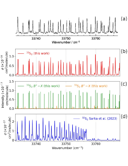
Figure 7: Comparison in the region of the $B-X$ (5,0) band of S2. (a) Laser induced fluorescence spectrum of S2 with rotational temperature of $\sim$300 K (reprinted from Fig. 6 of Green and Western (1996), with the permission of AIP Publishing). (b) Experimental absorption cross section at 300 K calculated using the line list from this work and convolved with a 0.1 cm^-1 Gaussian lineshape. (c) Line positions and intensities from the HITRAN-formatted line list of this work showing the $B-X$ and weaker $B^{\prime\prime}-X$ lines. (d) Experimental absorption cross section at 300 K from the Supplementary Material of Sarka and Nanbu (2023) convolved with a 0.1 cm^-1 Gaussian lineshape.

The $B^{\prime\prime}-X$ transition is included in our line list since the two $B$ and $B^{\prime\prime}$ states are heavily mixed (Green and Western, 1997). In particular, the mixing between the $B$ and $B^{\prime\prime}$ states occurs strongly where the $B$ $v^{\prime}$=7-9 bands are located. The $B^{\prime\prime}-X$ transition is applied as a perturbation in the PGOPHER file, so no oscillator strengths are applied, and the intensities are borrowed from the $B-X$ transition. This gives rise to $B-X$ and $B^{\prime\prime}-X$ bands with high vibrational levels for both $v^{\prime}$ and $v^{\prime\prime}$. Given that these states will be expected to have small populations, we have restricted the HITRAN-formatted line list for the $B-X$ tradition to $v^{\prime}\leq 3$ and $v^{\prime\prime}\leq 10$ below the dissociation limit and to $v^{\prime}\leq 27$ and $v^{\prime\prime}\leq 2$ above the dissociation limit (see Fig. 4). The excluded bands can be recalculated using the PGOPHER file in the Supplementary Material.

There are no reported partition functions available for comparison in the literature. From a qualitative comparison with Figure 5 of van der Heijden and van der Mullen (2001) one can tell that the partition sum from our work, is multiple times larger at 1000 K, due to the necessary inclusion of spin-splitting in our model. On a related note, since our model includes energy levels up to $J_{\textrm{max}}=150$ and $v_{\textrm{max}}=10$ for the ground state, we advise caution at temperatures beyond 1500 K as we expect the partition sum to start to deviate from a complete partition function as temperature increases. The partition sum calculated for this work is included in the Supplementary Material.

Conclusions

  A HITRAN-formatted line list for S2 that covers the UV spectral range has been calculated from spectroscopic constants available in the literature (Green and Western, 1996, 1997; Lewis et al., 2018) using the PGOPHER program (Western, 2017) and a fit to line positions of emission bands with a standard deviation of 0.130 cm^-1. The line list includes the prominent $B\,^{3}\Sigma^{-}_{u}-X\,^{3}\Sigma^{-}_{g}$ electronic transition of ^32S2 with bands $v^{\prime}$=0-27 and $v^{\prime\prime}$=0-10. The perturbing electronic transition $B^{\prime\prime}\,{}^{3}\Pi_{u}-X\,^{3}\Sigma^{-}_{g}$ is also included, with $v^{\prime}$=0-19, $v^{\prime\prime}$=0-10. The line list is provided as Supplementary Material in the commonly-used HITRAN format and will also be freely available online at https://hitran.org/.

Line intensities for predissociated bands have been obtained by fitting to the experimental observations of Stark et al. (2018). The line list has been validated through comparisons to existing experimental cross-section spectra for the predissociated region. The predissociation of S2 for $v^{\prime}\geq$10 in the $B-X$ transition requires the inclusion of predissociation line widths. Therefore, a Python program has been developed to be used in conjunction with HAPI that can apply the necessary predissociation line widths when using the HITRAN-formatted line list provided in the Supplementary Material. Currently, HAPI does not have the functionality to include predissociation line widths. However, it is planned that the program will be incorporated into future versions.

Our S2 line list can be used for exoplanet and planetary atmospheric investigations and photochemical models. The inclusion of our S2 line list in photochemical models is expected to improve atmospheric interpretations of planetary spectra that have previously been based on estimates. In particular, interpretations of the JWST spectra of WASP-39b expect S2 to be a key molecule in the formation of SO2.

It should be noted that in May 2023, the Leiden database Heays et al. (2017) updated their S2 cross-sections to include a preliminary version of the data reported here (see Hrodmarsson and Van Dishoeck, 2023), but temperature independence still remains. The S2 line list reported in this work provides greater flexibility for temperature coverage.

In addition to new experiments (especially for minor isotopologues), in future works, ab initio calculations (after validation) can help improve line lists of the sulfur dimer. The work of Sarka and Nanbu (2023) is an important step in that direction. In principle, ab initio methods can be used to calculate line positions and intensities, but may still be deficient for perturbations. They can also provide information on the predissociation widths and continuum contribution (see review by Tennyson et al., 2023).

In summary, we provide a publicly available S2 line list and associated calculation tools, which can be used to simulate the emission and absorption spectrum of ^32S2 over the 21 700$-$41 300 cm^-1 ($\sim$242$-$461 nm) spectral range.

Conflicts of Interest

  The authors declare that they have no known competing financial interests or personal relationships that could have appeared to influence the work reported in this paper. The funders had no role in the design of the study; in the collection, analyses, or interpretation of data; in the writing of the manuscript, or in the decision to publish the results.

Bibliography

Bibliography

- A’Hearn et al. (1983) A’Hearn, M.F., Schleicher, D.G., Feldman, P.D., 1983. The discovery of \chS2 in comet IRAS-Araki-Alcock 1983d. The Astrophysical Journal 274, L99–L103. doi:10.1086/184158.
- Anderson et al. (1979) Anderson, W.R., Crosley, D.R., Allen, J.E., 1979. Franck-Condon factors for the B-X system of S2. Journal of Chemical Physics 71, 821–829. doi:10.1063/1.438372.
- Barrow and Yee (1974) Barrow, R.F., Yee, K.K., 1974. The 3- ground states of the group VI–VI molecules, O2, SO, Te2. Acta Physica Academiae Scientiarum Hungaricae 35, 239. doi:10.1007/BF031597601.
- Bernath (2016) Bernath, P.F., 2016. Spectra of Atoms and Molecules. Third ed., Oxford University Press, New York.
- da Silva and Ballester (2019) da Silva, R.S., Ballester, M.Y., 2019. Potential energy curves, turning points, Franck-Condon factors and r-centroids for the astrophysically interesting S2 molecule. Astrophysics and Space Science 364, 169. doi:10.1007/s10509-019-3656-3.
- de Almeida and Singh (1986) de Almeida, A.A., Singh, P.D., 1986. Photodissociation lifetime of 32\chS2 molecule in comets. Earth Moon and Planets 36, 117–125. doi:10.1007/BF00057603.
- De Biévre et al. (1984) De Biévre, P., Gallet, M., Holden, N.E., Barnes, I.L., 1984. Isotopic Abundances and Atomic Weights of the Elements. Journal of Physical and Chemical Reference Data 13, 809–891. doi:10.1063/1.555720.
- Fink et al. (1986) Fink, E.H., Kruse, H., Ramsay, D.A., 1986. The high-resolution emission spectrum of S2 in the near infrared: The b1g+- X3g- system. Journal of Molecular Spectroscopy 119, 377–387. doi:10.1016/0022-2852(86)90032-9.
- Francés-Monerris et al. (2022) Francés-Monerris, A., Carmona-García, J., Trabelsi, T., Saiz-Lopez, A., Lyons, J.R., Francisco, J.S., Roca-Sanjuán, D., 2022. Photochemical and thermochemical pathways to S2 and polysulfur formation in the atmosphere of Venus. Nature Communications 13, 4425. doi:10.1038/s41467-022-32170-x.
- Gamache et al. (2021) Gamache, R.R., Vispoel, B., Rey, M., Nikitin, A., Tyuterev, V., Egorov, O., Gordon, I.E., Boudon, V., 2021. Total internal partition sums for the HITRAN2020 database. Journal of Quantitative Spectroscopy and Radiative Transfer 271, 107713. URL: https://zenodo.org/record/4708099, doi:10.1016/j.jqsrt.2021.107713.
- Gordon et al. (2016) Gordon, I.E., Potterbusch, M.R., Bouquin, D., Erdmann, C.C., Wilzewski, J.S., Rothman, L.S., 2016. Are your spectroscopic data being used? Journal of Molecular Spectroscopy 327, 232–238. URL: https://www.sciencedirect.com/science/article/pii/S0022285216300388, doi:10.1016/J.JMS.2016.03.011.
- Gordon et al. (2022) Gordon, I.E., Rothman, L.S., Hargreaves, R.J., Hashemi, R., Karlovets, E.V., Skinner, F.M., Conway, E.K., Hill, C., Kochanov, R.V., Tan, Y., Wcisło, P., Finenko, A.A., Nelson, K., Bernath, P.F., Birk, M., Boudon, V., Campargue, A., Chance, K.V., Coustenis, A., Drouin, B.J., Flaud, J.M., Gamache, R.R., Hodges, J.T., Jacquemart, D., Mlawer, E.J., Nikitin, A.V., Perevalov, V.I., Rotger, M., Tennyson, J., Toon, G.C., Tran, H., Tyuterev, V.G., Adkins, E.M., Baker, A., Barbe, A., Canè, E., Császár, A.G., Dudaryonok, A., Egorov, O., Fleisher, A.J., Fleurbaey, H., Foltynowicz, A., Furtenbacher, T., Harrison, J.J., Hartmann, J.M., Horneman, V.M., Huang, X., Karman, T., Karns, J., Kassi, S., Kleiner, I., Kofman, V., Kwabia–Tchana, F., Lavrentieva, N.N., Lee, T.J., Long, D.A., Lukashevskaya, A.A., Lyulin, O.M., Makhnev, V.Y., Matt, W., Massie, S.T., Melosso, M., Mikhailenko, S.N., Mondelain, D., Müller, H.S.P., Naumenko, O.V., Perrin, A., Polyansky, O.L., Raddaoui, E., Raston, P.L., Reed, Z.D., Rey, M., Richard, C., Tóbiás, R., Sadiek, I., Schwenke, D.W., Starikova, E., Sung, K., Tamassia, F., Tashkun, S.A., Vander Auwera, J., Vasilenko, I.A., Vigasin, A.A., Villanueva, G.L., Vispoel, B., Wagner, G., Yachmenev, A., Yurchenko, S.N., 2022. The HITRAN2020 molecular spectroscopic database. Journal of Quantitative Spectroscopy and Radiative Transfer 277, 107949. doi:10.1016/j.jqsrt.2021.107949.
- Green and Western (1997) Green, M., Western, C., 1997. Upper vibrational states of the B state of . Journal of the Chemical Society, Faraday Transactions 93, 365–372. doi:10.1039/A606591K.
- Green and Western (1996) Green, M.E., Western, C.M., 1996. A deperturbation analysis of the B (=0-6) and the B (=2-12) states of \chS2. Journal of Chemical Physics 104. doi:10.1063/1.470810.
- Heaven et al. (1984) Heaven, M., Miller, T.A., Bondybey, V.E., 1984. Chemical formation and spectroscopy of S2 in a free jet expansion. The Journal of Chemical Physics 80, 51–56. doi:10.1063/1.446424.
- Heays et al. (2017) Heays, A.N., Bosman, A.D., Van Dishoeck, E.F., 2017. Photodissociation and photoionisation of atoms and molecules of astrophysical interest. Astronomy & Astrophysics 602, A105. URL: https://www.aanda.org/articles/aa/full_html/2017/06/aa28742-16/aa28742-16.htmlhttps://www.aanda.org/articles/aa/abs/2017/06/aa28742-16/aa28742-16.html, doi:10.1051/0004-6361/201628742, arXiv:1701.04459.
- Hobbs et al. (2021) Hobbs, R., Rimmer, P.B., Shorttle, O., Madhusudhan, N., 2021. Sulfur chemistry in the atmospheres of warm and hot Jupiters. Monthly Notices of the Royal Astronomical Society 506, 3186--3204. URL: https://academic.oup.com/mnras/article/506/3/3186/6311826, doi:10.1093/MNRAS/STAB1839, arXiv:2101.08327.
- Hrodmarsson and Van Dishoeck (2023) Hrodmarsson, H.R., Van Dishoeck, E.F., 2023. Photodissociation and photoionization of molecules of astronomical interest - Updates to the Leiden photodissociation and photoionization cross section database. Astronomy & Astrophysics 675, A25. URL: https://www.aanda.org/articles/aa/full_html/2023/07/aa46645-23/aa46645-23.htmlhttps://www.aanda.org/articles/aa/abs/2023/07/aa46645-23/aa46645-23.html, doi:10.1051/0004-6361/202346645.
- Hu et al. (2012) Hu, R., Seager, S., Bains, W., 2012. Photochemistry in Terrestrial Exoplanet Atmospheres. I. Photochemistry Model and Benchmark Cases. The Astrophysical Journal 761, 166. doi:10.1088/0004-637X/761/2/166.
- Huber and Herzberg (1979) Huber, K.P., Herzberg, G.H., 1979. Constants of Diatomic Molecules. Van Nostrand, New York, (data prepared by Jean W. Gallagher and Russell D. Johnson, III) in NIST Chemistry WebBook, NIST Standard Reference Database Number 69, Eds. P.J. Linstrom and W.G. Mallard, National Institute of Standards and Technology, Gaithersburg MD, 20899, https://doi.org/10.18434/T4D303.
- Ikenoue (1953) Ikenoue, K., 1953. The Rotational Structure of the Band Spectrum of S2 Molecule. Part I. Journal of the Physical Society of Japan 8, 646--652. URL: https://journals.jps.jp/doi/abs/10.1143/JPSJ.8.646https://journals.jps.jp/doi/10.1143/JPSJ.8.646, doi:10.1143/JPSJ.8.646.
- Ikenoue (1960) Ikenoue, K., 1960. The Rotational Structure of the Band Spectrum of S2 Molecule. Part II. Science of Light 9, 79--98.
- JWST Transiting Exoplanet Community Early Release Science Team et al. (2023) JWST Transiting Exoplanet Community Early Release Science Team, Ahrer, E.M., Alderson, L., Batalha, N.M., Batalha, N.E., Bean, J.L., Beatty, T.G., Bell, T.J., Benneke, B., Berta-Thompson, Z.K., Carter, A.L., Crossfield, I.J.M., Espinoza, N., Feinstein, A.D., Fortney, J.J., Gibson, N.P., Goyal, J.M., Kempton, E.M.R., Kirk, J., Kreidberg, L., López-Morales, M., Line, M.R., Lothringer, J.D., Moran, S.E., Mukherjee, S., Ohno, K., Parmentier, V., Piaulet, C., Rustamkulov, Z., Schlawin, E., Sing, D.K., Stevenson, K.B., Wakeford, H.R., Allen, N.H., Birkmann, S.M., Brande, J., Crouzet, N., Cubillos, P.E., Damiano, M., Désert, J.M., Gao, P., Harrington, J., Hu, R., Kendrew, S., Knutson, H.A., Lagage, P.O., Leconte, J., Lendl, M., MacDonald, R.J., May, E.M., Miguel, Y., Molaverdikhani, K., Moses, J.I., Murray, C.A., Nehring, M., Nikolov, N.K., Petit dit de la Roche, D.J.M., Radica, M., Roy, P.A., Stassun, K.G., Taylor, J., Waalkes, W.C., Wachiraphan, P., Welbanks, L., Wheatley, P.J., Aggarwal, K., Alam, M.K., Banerjee, A., Barstow, J.K., Blecic, J., Casewell, S.L., Changeat, Q., Chubb, K.L., Colón, K.D., Coulombe, L.P., Daylan, T., de Val-Borro, M., Decin, L., Dos Santos, L.A., Flagg, L., France, K., Fu, G., García Muñoz, A., Gizis, J.E., Glidden, A., Grant, D., Heng, K., Henning, T., Hong, Y.C., Inglis, J., Iro, N., Kataria, T., Komacek, T.D., Krick, J.E., Lee, E.K.H., Lewis, N.K., Lillo-Box, J., Lustig-Yaeger, J., Mancini, L., Mandell, A.M., Mansfield, M., Marley, M.S., Mikal-Evans, T., Morello, G., Nixon, M.C., Ortiz Ceballos, K., Piette, A.A.A., Powell, D., Rackham, B.V., Ramos-Rosado, L., Rauscher, E., Redfield, S., Rogers, L.K., Roman, M.T., Roudier, G.M., Scarsdale, N., Shkolnik, E.L., Southworth, J., Spake, J.J., Steinrueck, M.E., Tan, X., Teske, J.K., Tremblin, P., Tsai, S.M., Tucker, G.S., Turner, J.D., Valenti, J.A., Venot, O., Waldmann, I.P., Wallack, N.L., Zhang, X., Zieba, S., 2023. Identification of carbon dioxide in an exoplanet atmosphere. Nature 614, 649--652. doi:10.1038/s41586-022-05269-w, arXiv:2208.11692.
- Kasting et al. (1989) Kasting, J.F., Zahnle, K.J., Pinto, J.P., Young, A.T., 1989. Sulfur, ultraviolet radiation, and the early evolution of life. Origins of Life and Evolution of the Biosphere 19, 95--108. doi:10.1007/BF01808144.
- Kim (1994) Kim, S.J., 1994. Ultraviolet and Visible Spectroscopic Database for Atoms and Molecules in Celestial Objects. Publications of The Korean Astronomical Society 9, 111--166.
- Kim et al. (2003) Kim, S.J., A’Hearn, M.F., Wellnitz, D.D., Meier, R., Lee, Y.S., 2003. The rotational structure of the B-X system of sulfur dimers in the spectra of Comet Hyakutake (C/1996 B2). Icarus 166, 157--166. doi:10.1016/j.icarus.2003.07.003.
- Kochanov et al. (2016) Kochanov, R.V., Gordon, I.E., Rothman, L.S., Wcisło, P., Hill, C., Wilzewski, J.S., 2016. HITRAN Application Programming Interface (HAPI): A comprehensive approach to working with spectroscopic data. Journal of Quantitative Spectroscopy and Radiative Transfer 177, 15--30. doi:10.1016/j.jqsrt.2016.03.005.
- Laffont et al. (1998) Laffont, C., Boice, D., Moreels, G., Clairemidi, J., Rousselot, P., Andernach, H., 1998. Tentative identification of \chS2 in the iue spectra of comet hyakutake (c/1996 b2). Geophysical research letters 25, 2749--2752. doi:10.1029/98GL01953.
- Lewis et al. (2018) Lewis, B., Gibson, S., Stark, G., Heays, A., 2018. Predissociation of the B state of \chS2: A coupled-channel model. The Journal of Chemical Physics 148, 244303. doi:10.1063/1.5029930.
- Matsumi et al. (1984) Matsumi, Y., Munakata, T., Kasuya, T., 1984. Direct observation of the B"3u–X3g transition of diatomic sulfur in a supersonic free jet. The Journal of Chemical Physics 81, 1108. URL: https://aip.scitation.org/doi/abs/10.1063/1.447804, doi:10.1063/1.447804.
- Matsumi et al. (1985) Matsumi, Y., Suzuki, T., Munakata, T., Kasuya, T., 1985. Time resolved study of the B3u and B"3u states of diatomic sulfur in a supersonic free jet. The Journal of Chemical Physics 83, 3798. URL: https://aip.scitation.org/doi/abs/10.1063/1.449142, doi:10.1063/1.449142.
- Meakin and Barrow (1962) Meakin, J.E., Barrow, R.F., 1962. The Electronic Spectrum of S2. Canadian Journal of Physics 40, 377--379. URL: http://www.nrcresearchpress.com/doi/10.1139/p62-040, doi:10.1139/p62-040.
- Naudé and Christy (1931) Naudé, S.M., Christy, A., 1931. The rotational analysis of the S2 bands. Phys. Rev. 37, 490--506. URL: https://link.aps.org/doi/10.1103/PhysRev.37.490, doi:10.1103/PhysRev.37.490.
- Noll et al. (1995) Noll, K.S., McGrath, M.A., Trafton, L.M., Atreya, S.K., Caldwell, J.J., Weaver, H.A., Yelle, R.V., Barnet, C., Edgington, S., 1995. HST Spectroscopic Observations of Jupiter After the Collision of Comet Shoemaker-Levy 9. Science 267, 1307--1313. doi:10.1126/science.7871428.
- Olsson (1936) Olsson, E., 1936. Das Bandenspektrum des Schwefels. Zeitschrift für Physik 100, 656--664. URL: https://link.springer.com/article/10.1007/BF01336723, doi:10.1007/BF01336723/METRICS.
- Patiño and Barrow (1982) Patiño, P., Barrow, R.F., 1982. Observations on the B and B states of s2. Journal of the Chemical Society, Faraday Transactions 2: Molecular and Chemical Physics 78, 1271--1282. doi:10.1039/F29827801271.
- Pradhan and Partridge (1996) Pradhan, A.D., Partridge, H., 1996. Theoretical study of the B3u--X 3g- and B-X 3g- band systems of S2. Chemical Physics Letters 255, 163--170. doi:10.1016/0009-2614(96)00363-6.
- Rustamkulov et al. (2022) Rustamkulov, Z., Sing, D.K., Mukherjee, S., May, E.M., Kirk, J., Schlawin, E., Line, M.R., Piaulet, C., Carter, A.L., Batalha, N.E., Goyal, J.M., López-Morales, M., Lothringer, J.D., MacDonald, R.J., Moran, S.E., Stevenson, K.B., Wakeford, H.R., Espinoza, N., Bean, J.L., Batalha, N.M., Benneke, B., Berta-Thompson, Z.K., Crossfield, I.J.M., Gao, P., Kreidberg, L., Powell, D.K., Cubillos, P.E., Gibson, N.P., Leconte, J., Molaverdikhani, K., Nikolov, N.K., Parmentier, V., Roy, P., Taylor, J., Turner, J.D., Wheatley, P.J., Aggarwal, K., Ahrer, E., Alam, M.K., Alderson, L., Allen, N.H., Banerjee, A., Barat, S., Barrado, D., Barstow, J.K., Bell, T.J., Blecic, J., Brande, J., Casewell, S., Changeat, Q., Chubb, K.L., Crouzet, N., Daylan, T., Decin, L., Désert, J., Mikal-Evans, T., Feinstein, A.D., Flagg, L., Fortney, J.J., Harrington, J., Heng, K., Hong, Y., Hu, R., Iro, N., Kataria, T., Kempton, E.M.R., Krick, J., Lendl, M., Lillo-Box, J., Louca, A., Lustig-Yaeger, J., Mancini, L., Mansfield, M., Mayne, N.J., Miguel, Y., Morello, G., Ohno, K., Palle, E., Petit dit de la Roche, D.J.M., Rackham, B.V., Radica, M., Ramos-Rosado, L., Redfield, S., Rogers, L.K., Shkolnik, E.L., Southworth, J., Teske, J., Tremblin, P., Tucker, G.S., Venot, O., Waalkes, W.C., Welbanks, L., Zhang, X., Zieba, S., 2022. Early Release Science of the exoplanet WASP-39b with JWST NIRSpec PRISM. arXiv e-prints , arXiv:2211.10487arXiv:2211.10487.
- Sarka and Nanbu (2023) Sarka, K., Nanbu, S., 2023. Potential Energy Curves and Ultraviolet Absorption Cross Sections of Sulfur Dimer. ACS Earth and Space Chemistry 0, in press. URL: https://doi.org/10.1021/acsearthspacechem.3c00116, doi:10.1021/acsearthspacechem.3c00116, arXiv:https://doi.org/10.1021/acsearthspacechem.3c00116.
- Setzer et al. (2003) Setzer, K.D., Kalb, M., Fink, E.H., 2003. The a1g → X3g- magnetic dipole transition of S2. Journal of Molecular Spectroscopy 221, 127--130. doi:10.1016/S0022-2852(03)00174-7.
- Shingledecker et al. (2020) Shingledecker, C.N., Lamberts, T., Laas, J.C., Vasyunin, A., Herbst, E., Kästner, J., Caselli, P., 2020. Efficient Production of S8 in Interstellar Ices: The Effects of Cosmic-Ray-driven Radiation Chemistry and Nondiffusive Bulk Reactions. The Astrophysical Journal 888, 52. URL: https://iopscience.iop.org/article/10.3847/1538-4357/ab5360https://iopscience.iop.org/article/10.3847/1538-4357/ab5360/meta, doi:10.3847/1538-4357/AB5360, arXiv:1911.01239.
- Smith and Liszt (1971) Smith, W.H., Liszt, H.S., 1971. Franck-Condon factors and absolute oscillator strengths for NH, SiH, S2 and SO. Journal of Quantitative Spectroscopy and Radiative Transfer 11, 45--54. doi:10.1016/0022-4073(71)90160-9.
- Spencer et al. (2000) Spencer, J.R., Jessup, K.L., McGrath, M.A., Ballester, G.E., Yelle, R., 2000. Discovery of Gaseous S2 in Io’s Pele Plume. Science 288, 1208--1210. doi:10.1126/science.288.5469.1208.
- Stark et al. (2018) Stark, G., Herde, H., Lyons, J., Heays, A., de Oliveira, N., Nave, G., Lewis, B., Gibson, S., 2018. Fourier-transform-spectroscopic photoabsorption cross sections and oscillator strengths for the \chS2 B-X system. Journal of Chemical Physics 148, 244302. doi:10.1063/1.5029929.
- Sun et al. (2019) Sun, Z.F., Farooq, Z., Parker, D.H., Martin, P.J.J., Western, C.M., 2019. Photodissociation of \chS2 (X3g–, a1g, and b1g+) in the 320–205 nm Region. Journal of Physical Chemistry A 123, 6886--6896. doi:10.1021/acs.jpca.9b05350.
- Tennyson et al. (2023) Tennyson, J., Pezzella, M., Zhang, J., Yurchenko, S.N., 2023. Data structures for photoadsorption within the ExoMol project. RAS Techniques and Instruments 2, 231--237. doi:10.1093/rasti/rzad014, arXiv:2306.04497.
- Tsai et al. (2022) Tsai, S.M., Lee, E.K.H., Powell, D., Gao, P., Zhang, X., Moses, J., Hébrard, E., Venot, O., Parmentier, V., Jordan, S., Hu, R., Alam, M.K., Alderson, L., Batalha, N.M., Bean, J.L., Benneke, B., Bierson, C.J., Brady, R.P., Carone, L., Carter, A.L., Chubb, K.L., Inglis, J., Leconte, J., Lopez-Morales, M., Miguel, Y., Molaverdikhani, K., Rustamkulov, Z., Sing, D.K., Stevenson, K.B., Wakeford, H.R., Yang, J., Aggarwal, K., Baeyens, R., Barat, S., Borro, M.d.V., Daylan, T., Fortney, J.J., France, K., Goyal, J.M., Grant, D., Kirk, J., Kreidberg, L., Louca, A., Moran, S.E., Mukherjee, S., Nasedkin, E., Ohno, K., Rackham, B.V., Redfield, S., Taylor, J., Tremblin, P., Visscher, C., Wallack, N.L., Welbanks, L., Youngblood, A., Ahrer, E.M., Batalha, N.E., Behr, P., Berta-Thompson, Z.K., Blecic, J., Casewell, S.L., Crossfield, I.J.M., Crouzet, N., Cubillos, P.E., Decin, L., Désert, J.M., Feinstein, A.D., Gibson, N.P., Harrington, J., Heng, K., Henning, T., Kempton, E.M.R., Krick, J., Lagage, P.O., Lendl, M., Line, M., Lothringer, J.D., Mansfield, M., Mayne, N.J., Mikal-Evans, T., Palle, E., Schlawin, E., Shorttle, O., Wheatley, P.J., Yurchenko, S.N., 2022. Direct Evidence of Photochemistry in an Exoplanet Atmosphere. arXiv e-prints , arXiv:2211.10490arXiv:2211.10490.
- Ueno et al. (2009) Ueno, Y., Johnson, M.S., Danielache, S.O., Eskebjerg, C., Pandey, A., Yoshida, N., 2009. Geological sulfur isotopes indicate elevated OCS in the Archean atmosphere, solving faint young sun paradox. Proceedings of the National Academy of Science 106, 14784--14789. doi:10.1073/pnas.0903518106.
- van der Heijden and van der Mullen (2001) van der Heijden, H., van der Mullen, J., 2001. Semiclassical and quantum-mechanical descriptions of S2 molecular radiation. Journal of Physics B Atomic Molecular Physics 34, 4183--4201. doi:10.1088/0953-4075/34/21/309.
- Western (2017) Western, C.M., 2017. PGOPHER: A program for simulating rotational, vibrational and electronic spectra. Journal of Quantitative Spectroscopy and Radiative Transfer 186, 221--242. doi:10.1016/j.jqsrt.2016.04.010.
- Wheeler et al. (1998) Wheeler, M.D., Newman, S.M., Orr-Ewing, A.J., 1998. Predissociation of the B state of \chS2. Journal of Chemical Physics 108, 6594--6605. doi:10.1063/1.476074.
- Xing et al. (2020) Xing, W., Shi, D., Sun, J., 2020. Transition properties of the X3-g, A3u, A3+u, B, B3-u, and B′3g states of sulphur dimer. Journal of Quantitative Spectroscopy and Radiative Transfer 242, 106805. doi:10.1016/j.jqsrt.2019.106805.
- Xing et al. (2013) Xing, W., Shi, D., Sun, J., Liu, H., Zhu, Z., 2013. Extensive ab initio study of the electronic states of S2 molecule including spin-orbit coupling. Molecular Physics 111, 673--685. doi:10.1080/00268976.2012.741721.
- Zahnle et al. (1995) Zahnle, K., Mac Low, M.M., Lodders, K., Fegley, Bruce, J., 1995. Sulfur chemistry in the wake of comet Shoemaker-Levy 9. Geophysical Research Letters 22, 1593--1596. doi:10.1029/95GL01190.