Aberration compensation for the anamorphic triplet

Abstract

Compensation of the generalized spherical aberrations is discussed for the plane-symmetric and anamorphic optical systems. The compensation rules are derived for an economical three-component double-plane symmetric telescopic system containing two cylindrical mirrors and one toroidal lens. Anamorphic systems, which provide large magnifications in the two orthogonal directions, are presented.

1 Introduction

Anamorphic optical systems (OS), which possess a double-plane symmetry, have been investigated for many years [1, 2, 3, 4, 5, 6, 7] mainly due to their rich capabilities for the image formation. However, they also reveal copious structure of aberrations [1, 12, 8, 4, 9, 10, 11] that remain a subject of research. In particular, S. Yuan and J. Sasian have argued that, in the paraxial region, an anamorphic system can be treated as two associated rotationally symmetric OS, and derived for pure mirror systems the generalized ray-tracing equations that include the aberration terms up to the third order [9, 10]. Recently, the full set of the third order aberration coefficients was obtained for the systems of cylindrical mirrors or/and lenses directly from the calculation of the optical path difference without approximating these OS by the pairs of rotationally symmetric OS, and as a particular example a cylindrical analog of the Cassegrain telescope was considered [11].

In the present letter, we discuss the primary monochromatic aberrations for either anamorphic or plane-symmetric OS in Sect. 2 and obtain conditions for the aberration compensations in the XZ and YZ planes for the promising anamorphic OS in Sect. 3, and then we conclude.

2 Plane symmetries and GS aberrations

The transverse aberrations for paraxial rays propagating in the $Z$ direction through a generic system of cylindrical optical surfaces, which is symmetric under reflection in the $YZ$ plane and translationally invariant along the $Y$ axis, were obtained in Ref. [11] by extension of the classical methods based on direct calculation of the optical path difference [13]. We consider generalization of this system to a single-plane or double-plane symmetric OS. In the later case the $Z$ axis coincides with the crossing line of the two symmetry planes, and the OS may contain anamorphic surfaces, e.g., toroidal ones. The wave aberration function $W$ being the optical path difference between real and intended ideal wavefronts [14] can be expressed in terms of the four transverse coordinates {$x_{0}$, $y_{0}$, $x$, $y$} of the points $P_{0}(x_{0},y_{0},0)$ and $P(x,y,z)$, in which arbitrary paraxial ray crosses, respectively, the object plane and the exit pupil plane. The both planes are orthogonal to the $Z$ axis. Symmetry in either $XZ$ or $YZ$ plane as well as double-plane symmetry in both these planes leaves the following six second order invariants for the considered four variables

$$x_{0}^{2},\quad y_{0}^{2},\quad x^{2},\quad y^{2},\quad x_{0}x,\quad y_{0}y.$$ (1)

Then the fourth-order wave function contains

$$\left(\begin{pmatrix}6\\ 2\end{pmatrix}\right)=\begin{pmatrix}6+2-1\\ 2\end{pmatrix}=\frac{7\times 6}{2}=21$$ (2)

quadratic combinations with repetition, of which there are three constant piston terms (involving only $x_{0}$ and $y_{0}$) and two pairs of identical terms with either $x_{0}^{2}x^{2}$ or $y_{0}^{2}y^{2}$. This leaves in the fourth-order wave aberration function

$$W^{(4)} =a_{1}x^{4}+a_{2}y^{4}+a_{3}x^{2}y^{2}$$

$$+a_{4}x_{0}x^{3}+a_{5}y_{0}x^{2}y+a_{6}x_{0}xy^{2}+a_{7}y_{0}y^{3}$$

$$+a_{8}x_{0}^{2}x^{2}+a_{9}y_{0}^{2}y^{2}+a_{10}y_{0}^{2}x^{2}+a_{11}x_{0}^{2}y^{2}+a_{12}x_{0}y_{0}xy$$

$$+a_{13}x_{0}^{3}x+a_{14}y_{0}^{3}y+a_{15}x_{0}y_{0}^{2}x+a_{16}x_{0}^{2}y_{0}y$$ (3)

sixteen different terms that generate the same number of primary (third-order) aberrations of spherical, comatic, astigmatic (plus field curvature) and distortion types, corresponding to the lines in (2) [15, 16, 17]. For paraxial rays the components of the primary transverse aberrations can be calculated as

$$\delta_{1x}=-\frac{D}{n}\frac{\partial W^{(4)}}{\partial x},\qquad\delta_{1y}=-\frac{D}{n}\frac{\partial W^{(4)}}{\partial y},$$ (4)

where $D$ is the distance between the exit pupil plane and the image plane, and $n$ is the refractive index of the material behind the exit pupil. In particular, the generalized spherical (GS) aberrations are given by

$$n\delta_{1x}^{e} = (\tilde{a}_{1}x^{2}+\tilde{a}_{3}y^{2})x,$$ (5)

$$n\delta_{1y}^{e} = (\tilde{a}_{3}x^{2}+\tilde{a}_{2}y^{2})y,$$ (6)

where $\tilde{a}_{1,2}=4a_{1,2}D$, $\tilde{a}_{3}=2a_{3}D$. Clearly, in the case of a single-plane or double-plane symmetry GS aberrations depend on three parameters, which is similar to the case of a single-plane symmetry combined with translation [11]. The GS aberrations degenerate to the ordinary spherical aberration for $\tilde{a}_{1}=\tilde{a}_{2}=\tilde{a}_{3}$.

We notice that for generic OS without the above symmetry restrictions the wave aberration function contains five fourth-order power products of the variables $x$ and $y$: $x^{4}$, $x^{3}y$, $x^{2}y^{2}$, $xy^{3}$ and $y^{4}$. Therefore five parameters can enter GS aberrations.

The conditions for GS aberration compensation for the rays propagating in the $XZ$ and $YZ$ planes nullify the coefficients $\tilde{a}_{1}$ and $\tilde{a}_{2}$, respectively. This can be easily seen from Eqs. (5) and (6) rewritten in the polar coordinates

$$x=\rho\cos\theta,\qquad y=\rho\sin\theta,$$ (7)

since the discussed conditions fix $\theta$ to be equal to either $k\pi$ or $\pi/2+k\pi$ with the integer $k$. However, the remaining parameter $\tilde{a}_{3}$ enters the quadrifolium (clover) component of GS aberrations:

$$n\delta_{1x}^{e} =a\sin^{2}\theta\cos\theta=\frac{a}{2}\sin 2\theta\sin\theta,$$ (8)

$$n\delta_{1y}^{e} =a\cos^{2}\theta\sin\theta=\frac{a}{2}\sin 2\theta\cos\theta,$$ (9)

where $a=\tilde{a}_{3}\rho^{3}$, as shown in Fig. 1 using Mathematica [18]. Compensation of this component requires a third condition (and two more parameters should be eliminated in the generic case).

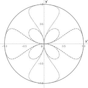
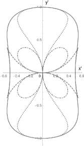
Figure 1: Generalized spherical aberrations for $a=1$ and the following chosen values for the parameter set {$\tilde{a}_{1}\rho^{3}$, $\tilde{a}_{2}\rho^{3}$} in Eqs. (5)-(7). Left: {1, 1} (solid), {1, 0} (dashed), {0, 1} (dotted) and {0, 0} (dot-dashed). Right: {$\tilde{a}_{1}\rho^{3}$, $\tilde{a}_{2}\rho^{3}$} set: {0.5, 1} (solid), {0.5, 0} (dashed), {0, 1} (dotted) and {0, 0} (dot-dashed).

3 GS aberrations for anamorphic triplet

We consider economical extension of the cylindrical OS of the Cassegrain type [11] to form a narrow-field-of-view anamorphic telescope (see the author’s patent application Nr. P.444521 submitted to the Patent Office of the Republic of Poland on April 21, 2023). Namely, we add a concave toroidal lens L to the OS consisting of the two cylindrical mirrors: concave primary M1 and convex secondary M2, as shown in Fig. 2. The two mirrors form the cylindrical set (I) and the lens is the only element in its anamorphic extension (II) that breaks the translational invariance of the OS to the second plane symmetry. The set (I) and its extension (II) are responsible for the focusing in $XZ$ and $YZ$ planes, respectively. The focal segment $AB$ of the primary M1 is parallel to the focal segment $A_{2}B_{2}$ of the secondary M2, and the symmetry axis of L coincides with the focal segment $A^{\prime}B^{\prime}$ of the cylindrical set (I). The OS focal point $C$ is in the center of the segment $A^{\prime}B^{\prime}$.

The discussed anamorphic triplet contains the four optical surfaces, indexed by 1 and 2 for M1 and M2, respectively, and 3 and 4 for L. We describe the cylindrical surfaces by the equation

$$z=\pm\left[\frac{x^{2}}{2R_{i}}+(1+\kappa_{i})\frac{x^{4}}{8R_{i}^{3}}\right],$$ (10)

where $R_{i}$ and $\kappa_{i}$ are the $i$-th surface’s radius of curvature and conic constant, respectively, overall sign determines the direction of the surface convexity, and the only asphericity is in $1+\kappa_{i}$.

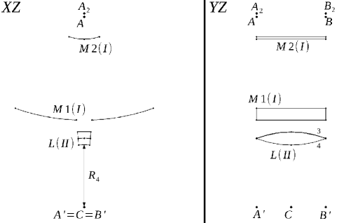
Figure 2: The discussed three-component anamorphic system in the projections of $XZ$ (left) and $YZ$ (right).

In the following subsections we introduce the conditions for GS aberration compensation for the considered anamorphic OS in the $XZ$ and $YZ$ planes, which correspond to the dotted and dashed lines in Fig. 1, respectively, where the dot-dashed line corresponds to the fulfillment of the both conditions at once.

3.1 $XZ$ plane

For the rays in the $XZ$ plane and the marginal ray height at the primary the contribution to GS aberration for the system is determined in terms of Ref. [11] by the function

$$A_{3s}^{(1)}=A_{311}+A_{312}\left(\frac{x_{2}}{x_{1}}\right)^{4}+A_{313}\left(\frac{x_{3}}{x_{1}}\right)^{4}+A_{314}\left(\frac{x_{4}}{x_{1}}\right)^{4},$$ (11)

where $x_{i}$ is the marginal ray height at the $i$-th surface. The aberration coefficients for the mirrors are given by

$$A_{311}=-\frac{\kappa_{1}+1}{4R_{1}^{3}},\qquad A_{312}=\frac{1}{4R_{2}^{3}}\left[\kappa_{2}+\left(\frac{\mu+1}{\mu-1}\right)^{2}\right],$$ (12)

where $\mu>0$ is the transverse magnification of the secondary.

To derive the aberration coefficients $A_{313}$ and $A_{314}$ we approximate the refractive surfaces 3 and 4 by the cylindrical ones, which are tangential to them in the $XZ$ plane and are described by (10) with the overall plus sign. Then we use the result of

$$A_{31}=-\,\frac{n_{0}}{8}\left[\frac{\kappa}{R^{3}}\frac{n_{1}-n_{0}}{n_{0}}+\frac{1}{s_{0}}\left(1+\frac{n_{0}}{n_{1}}\frac{s_{0}}{s_{1}}\right)\left(\frac{1}{s_{0}}+\frac{1}{R}\right)^{2}\right]$$ (13)

from Table 2 in Ref. [11] for $b=0$. The $XZ$ projections for the 3rd and 4th surfaces are the circle arcs with the radii $R_{3}$ and $R_{4}$, respectively, which are centered in the OS focal point $C$, see Fig. 2 (left). We take the refractive index to be $n$ inside the lens and unity outside. For $\kappa_{3}=\kappa_{4}=0$ we obtain

$$A_{313} = -\,\frac{1}{8s_{03}}\left(1+\frac{s_{03}}{ns_{13}}\right)\left(\frac{1}{s_{03}}+\frac{1}{R_{3}}\right)^{2},$$ (14)

$$A_{314} = -\,\frac{n}{8s_{04}}\left(1+\frac{ns_{04}}{s_{14}}\right)\left(\frac{1}{s_{04}}+\frac{1}{R_{4}}\right)^{2},$$ (15)

where $s_{0i}$ and $s_{1i}$ are the chief ray segments connecting the $i$-th surface with the object and the image, respectively. Using the rule of ‘negative distance’ between a surface and a virtual object (concave beam), we write

$$s_{0j}=-s_{1j}=-R_{j}$$ (16)

for $j=3,4$, and the coefficients $A_{313}$ and $A_{314}$ vanish. Then the condition of compensation of GS aberrations for the discussed OS in the $XZ$ plane coincides with the one for isolated set (I) [11]:

$$F_{XZ}(\kappa_{1},\kappa_{2},\mu,\rho,k_{x})\equiv\kappa_{1}+1-\frac{k_{x}^{4}}{\rho^{3}}\left[\kappa_{2}+\left(\frac{\mu+1}{\mu-1}\right)^{2}\right]=0,$$ (17)

where $\rho=R_{2}/R_{1}$ and $k_{x}=x_{2}/x_{1}$. In particular, for a telescope of classical Cassegrain type: $\kappa_{1}=-1$ (paraboloidal M1) and $\kappa_{2}=-(\mu+1)^{2}(\mu-1)^{-2}$ (hyperboloidal M2).

3.2 $YZ$ plane

The GS aberration component in the $YZ$ plane for the marginal ray height at the primary can be determined by

$$B_{3s}^{(1)}=\tilde{B}_{31}+\tilde{B}_{32}\left(\frac{y_{2}}{y_{1}}\right)^{4}+B_{33}\left(\frac{y_{3}}{y_{1}}\right)^{4}+B_{34}\left(\frac{y_{4}}{y_{1}}\right)^{4},$$ (18)

where $y_{i}$ is the marginal ray distance from the $Z$ axis at the $i$-th surface. The aberration coefficients $\tilde{B}_{3i}=A_{32i}$, using the relation of $s_{02}=-f_{1}x_{2}/x_{1}$ (negative for convex mirror) with the focal length $f_{1}$ of the primary, can be written as [11]

$$\tilde{B}_{31}=\frac{1}{8f_{1}^{3}},\qquad\tilde{B}_{32}=-\frac{x_{1}^{3}}{8x_{2}^{3}f_{1}^{3}}\,\frac{1-4\mu+6\mu^{2}-3\mu^{3}}{\mu^{3}}.$$ (19)

The coefficients $B_{33}$ and $B_{34}$ we find, using the approximation of the surfaces 3 and 4 by the cylinders, which are tangential to these surfaces in the $YZ$ plane and translationary invariant along the $X$ axis. This invariance interchanges the roles of $A\leftrightarrow B$ and $x_{i}\leftrightarrow y_{i}$ in Eqs. (113) and (119) of Ref. [11]. Taking into account the same form of these equations and substituting to (13) either $r_{3}$ or $-r_{4}$, according to the proper overall sign in (10), we have

$$B_{33}=-\,\frac{\kappa_{3y}(n-1)}{8r_{3}^{3}}-\frac{1}{8s_{03y}}\left(1+\frac{s_{03y}}{ns_{13y}}\right)\left(\frac{1}{s_{03y}}+\frac{1}{r_{3}}\right)^{2},$$ (20)

$$B_{34}=-\,\frac{\kappa_{4y}(n-1)}{8r_{4}^{3}}-\frac{n}{8s_{04y}}\left(1+\frac{ns_{04y}}{s_{14y}}\right)\left(\frac{1}{s_{04y}}-\frac{1}{r_{4}}\right)^{2},$$ (21)

where the quantities relevant to the $YZ$ plane are indexed by $y$, and $r_{i}\equiv R_{iy}$ is the radius of curvature of the $i$-th surface.

The thick lens equations [13] for the $YZ$ profile of $L$ read as

$$\frac{n}{s_{13y}}-\frac{1}{s_{03y}}=\frac{n-1}{r_{3}},\qquad\frac{1}{s_{14y}}-\frac{n}{s_{04y}}=\frac{1-n}{r_{4}}$$ (22)

with $s_{03y}=\infty$ and $s_{04y}=s_{13y}-d_{L}$, where the lens width $d_{L}$ can be calculated from the properties of surfaces 3 and 4 by

$$d_{L}=d_{3}+d_{4}=R_{3}-R_{4},$$ (23)

where width of an imaginary plano-convex component of the cylindrical lens, which is tangential to $L$ in the $YZ$ plane, is given by

$$d_{i}=r_{i}\left(1-\sqrt{1-\left(\frac{L_{y}}{2r_{i}}\right)^{2}}\right),$$ (24)

and $L_{y}=AB$ is the lens size along the $Y$ axis. Using Eqs. (22) and the relation of $s_{14y}=f_{L}-d_{4}$, we extract the lens focal distance as

$$f_{L}=d_{4}+\frac{r_{4}}{n-1}\,\frac{nr_{3}-(n-1)d_{L}}{n(r_{4}-r_{3})+(n-1)d_{L}}.$$ (25)

Now Eqs. (20) and (21) can be rewritten as

$$B_{33} =-\,\frac{n-1}{8r_{3}^{3}}\left(\kappa_{3y}+\frac{1}{n^{2}}\right),$$ (26)

$$B_{34} =\frac{1-n}{8}\left[\kappa_{4y}+\frac{n}{\sigma}\left(1+\frac{n}{n-1}\,\frac{\sigma}{f_{L}-d_{4}}\right)\left(\frac{n-1}{\sigma}-\frac{1}{r_{4}}\right)^{2}\right],$$ (27)

where $\sigma=nr_{3}-(n-1)d_{L}$. For $y_{i}=L_{y}/2$ in (18), the condition of compensation of GS aberrations in the $YZ$ plane reads

$$0 =-F_{YZ}(n,f_{1},\mu,k_{x},\kappa_{3y},\kappa_{4y},r_{3},r_{4},L_{y})\equiv-\frac{1}{(n-1)f_{1}^{3}}F_{YZ}^{(I)}(\mu,k_{x}\!)$$

$$+\frac{\kappa_{3y}}{r_{3}^{3}}+\frac{\kappa_{4y}}{r_{4}^{3}}+\frac{1}{n^{2}r_{3}^{3}}+\frac{n}{\sigma}\!\left(1+\frac{n}{n-1}\,\frac{\sigma}{f_{L}-d_{4}}\right)\!\left(\frac{n-1}{\sigma}-\frac{1}{r_{4}}\right)^{2}\!,$$ (28)

where $f_{L}(n,r_{3},r_{4},L_{y})$ is given by (25) and the function

$$F_{YZ}^{(I)}(\mu,k_{x})=1+\frac{3\mu^{3}-6\mu^{2}+4\mu-1}{k_{x}^{3}\mu^{3}},$$ (29)

which was obtained in Ref. [11], vanish in the case of similar aberration compensation for the isolated cylindrical set (I). In particular, for $\kappa_{3y}=\kappa_{4y}=0$ and $r_{3}=r_{4}\equiv r$ we get

$$f_{1}^{3}(n,\mu,k_{x},r,L_{y})=$$

$$\frac{F_{YZ}^{(I)}}{n-1}\!\left[\frac{1}{n^{2}r^{3}}+\frac{n}{\sigma}\!\left(1+\frac{n}{n-1}\,\frac{2\sigma}{2f_{L}-d_{L}}\!\right)\!\left(\frac{n-1}{\sigma}-\frac{1}{r}\right)^{2}\right]^{-1}\!\!\!$$ (30)

with $d_{L}=2d_{i}(r,L_{y})$,  $\sigma(n,r,L_{y})=nr-(n-1)d_{L}$ and

$$f_{L}(n,r,L_{y})=\frac{d_{L}}{2}+\frac{\sigma\,r}{(n-1)^{2}d_{L}}.$$ (31)

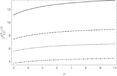
Figure 3: $F_{YZ}^{(I)}$ vs $\mu$. The solid, dashed, dotted and dot-dashed line represents the value of $k_{x}=0.1$, 0.15, 0.2 and 0.3, respectively.

For $r=\alpha L_{y}$ the ratio of $f_{1}/L_{y}$ is a constant with respect to $L_{y}$, while its dependence on $\mu$ and $k_{x}$ is factorized in the cubic root of $F_{YZ}^{(I)}(\mu,k_{x})$, which dependence on $\mu$ is shown in Fig. 3 for the selected values of $k_{x}$. The dependence of $f_{1}/L_{y}$ on $\alpha$ is shown in Fig. 4 for the typical values of $\mu=3$ and $k_{x}=0.2$, and for the chosen values of the refractive index. The (24) puts the limit of $\alpha\geq 1/2$. Position of global minimum of $f_{1}/L_{y}$ moves from $\alpha=0.54$ to $\alpha=0.5$ for $n$ decreasing below 1.55. Knowledge of $(f_{1}/L_{y})^{\rm min}$ can help in reduction of the telescope’s size. However, if the size $L_{x}$ of the mirror M1 in the $X$ direction is large with respect to $L_{y}$ then the discussed lower bound $f_{1}^{\rm min}$ on the primary’s focal length is not a problem. Also in this case the lens $L$ is small with respect to M1 and there is no essential loss-of-light.

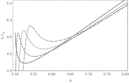
Figure 4: Ratio of $f_{1}/L_{y}$ vs $\alpha=r/L_{y}$ for $\mu=3$ and $k_{x}=0.2$. The solid, dashed, dotted and dot-dashed line represents the value of the refractive index $n$ of 1.5, 1.6, 1.7 and 1.8, respectively.

To achieve large magnifications in the mutually orthogonal directions $X$ and $Y$ one can use the schemes containing two cylindrical sets of elements, (I.a) and (I.b), as well as anamorphic set. The set (I.a) is similar to (I) in the scheme of Fig. 2, but works as a beam compressor in the $X$ direction (with $\kappa_{1}=\kappa_{2}$ its focal segments $AB$ and $A_{2}B_{2}$ coincide). The subsequent set (I.b) is analogous to (I), but is rotated by the angle $\pi/2$ with respect to the $Z$ axis and focuses the beam in the $YZ$ plane (to a focal segment orthogonal to this plane). The anamorphic set, which focuses the beam in the $XZ$ plane (to the OS focal point), may contain the anamorphic lens(es), e. g., a toroidal lens similar to the one in Fig. 2, but also rotated by 90^∘ with respect to the $Z$ axis. In particular, with $L_{x}^{a}\gg L_{y}^{a}$ for the set (I.a) and $L_{y}^{b}=L_{y}^{a}\gg L_{x}^{b}$ for the set (I.b) the size of lens(es) in the anamorphic set may not exceed $L_{x}^{b}$.

4 Conclusion

We briefly discussed the primary aberrations, mainly GS ones, for the OS possessing either single- or double-plane symmetry. We considered the aberration compensation for the three-element OS, which is a simple anamorphic extension of the cylindrical analog of the Cassegrain telescope. By approximating the toroidal surfaces by the cylindrical ones, which are tangential to them in the $XZ$ and $YZ$ planes, we obtained the conditions for compensation of GS aberration for the rays propagating in one of these planes, respectively. The remaining component of GS aberration is the clover aberration. Contributions to this component from the cylindrical surfaces can be described using the results of Ref. [11]. However, calculation of the contributions from anamorphic surfaces requires extended formulation and will be considered in the future works.

Fixation of several main parameters of an optical system by the requirement of compensation of selected aberrations (e. g., GS aberration components) reduces the number of parameters to be determined in the complete design of an anamorphic OS, causing essential simplification. The freedom in the remaining parameters can be used among other purposes for partial compensation of the remaining aberrations, which can be carried out analytically as well as numerically. More advanced design may include extra parameters describing the surfaces, e.g., higher order deformation coefficients: asphericities, acylindricities, etc.

Disclosures The author declares no conflicts of interest.

Data availability No data were generated or analyzed in the presented research.

References

- [1] H. Chretien, “Anamorphotic lens system and method of making the same”, U.S. patent 1,962,892 (1934).
- [2] T. Kasuya, T. Suzuki, and K. Shimoda, \JournalTitleApplied Physics 17, 131(1978).
- [3] J.-H. Jung, and J.-W. Lee, “Anamorphic lens for a CCD camera apparatus”, U.S. patent 5,671,093 (1997).
- [4] I. A. Neil, “Anamorphic imaging system”, U.S. patent 7,085,066 (2006).
- [5] T. Peschel et al., \JournalTitleProceedings of SPIE 10563, 105631Y-2 (2014).
- [6] S. Kashima et al., \JournalTitleApplied Optics 57, 4171(2018).
- [7] Y. Shi et al., \JournalTitlePhotonics 9 836 (2022).
- [8] M. Rusinov, “Composition of optical systems,” (L.: Mashinostroenie, 1989), ISBN: 5-217-00546-7.
- [9] S. Yuan and J. Sasian, \JournalTitleApplied Optics 48, 2574(2009).
- [10] S. Yuan, and J. Sasian, \JournalTitleApplied Optics 48, 2836(2009).
- [11] D. Zhuridov, \JournalTitleApplied Optics, https://doi.org/10.1364/AO.511270.
- [12] G. Slusarev, “Methods for calculating optical systems,” second edition (L.: Mashinostroenie, 1969).
- [13] D. J. Schroeder, “Astronomical Optics,” second edition (Academic Press 1999).
- [14] M. Born, and E. Wolf, “Principles of Optics,” sixth edition (Oxford: Pergamon, 1980).
- [15] J. C. Burfoot, \JournalTitleProceedings of the Physical Society B 67, 523(1954).
- [16] R. Barakat and A. Houston, \JournalTitleOptica Acta 13, 1(1966).
- [17] S. Yuan, “Aberrations of anamorphic optical systems”, Ph.D. dissertation (University of Arizona, 2008).
- [18] Wolfram Research, Inc., Mathematica, Version 11, Champaign, IL (2016).