Critical lengths of Steklov eigenvalues of hypersurfaces of revolution in Euclidean space

Abstract.

We study the Steklov problem on hypersurfaces of revolution with two boundary components in Euclidean space. In [10], the phenomenon of critical length, at which a Steklov eigenvalue is maximized, was exhibited and multiple questions were raised. In this article, we conjecture that, in any dimension, there is a finite number of infinite critical length. To investigate this, we develop an algorithm to efficiently perform numerical experiments, providing support to our conjecture. Furthermore, we prove the conjecture in dimension $n=3$ and $n=4$.

Keywords: Spectral geometry, Steklov problem, hypersurfaces of revolution, numerical experiments.

1. Introduction

Let $(M,g)$ a smooth compact connected Riemannian manifold of dimension $n\geq 2$ with smooth boundary $\Sigma$, the Steklov problem on $(M,\Sigma)$ consists in finding the real numbers $\sigma$ and the functions $f:M\longrightarrow\mathbb{R}$ such that

$$\left\{\begin{array}[]{c}\Delta f=0\mbox{ in }M\\ \partial_{\nu}f=\sigma f\mbox{ on }\Sigma,\end{array}\right.$$

where $\nu$ denotes the outward normal on $\Sigma$. Such a $\sigma$ is called a Steklov eigenvalue of $(M,g)$. It is well known that the Steklov spectrum forms a discrete sequence $0=\sigma_{0}(M,g)<\sigma_{1}(M,g)\leq\sigma_{2}(M,g)\leq\ldots\nearrow\infty$, where each eigenvalue is repeated with its multiplicity, which is finite.

Since we are interested in upper bounds for the Steklov eigenvalues of a family of manifolds, we have to add some geometric constraints on the manifolds. Indeed, [2, Theorem 1.1] states that if $(M,g)$ is a compact connected manifold of dimension $n\geq 3$ with boundary $\Sigma$, then there exists a family of Riemannian metrics $(g_{\varepsilon})$ conformal to $g$ and that agrees with $g$ on $\Sigma$ such that

$$\sigma_{1}(M,g)\longrightarrow\infty\;\mbox{ as }\;\varepsilon\longrightarrow 0.$$

A class of manifolds that was recently investigated consists of warped products of the form $[0,L]\times\mathbb{S}^{n-1}$, where $L$ is a positive real number and $\mathbb{S}^{n-1}$ is the unit sphere of dimension $n-1$, see for instance [7, 8, 11, 12]. Some authors studied the particular case where these warped products manifolds can be seen as hypersurfaces of revolution in Euclidean space, see [3, 4, 10]. In this article, we will focus in these hypersurfaces of revolution in Euclidean space. Let us start by recalling what they are.

Definition 1.

A $n$-dimensional compact hypersurface of revolution $(M,g)$ in Euclidean space with two boundary components is the warped product $M=[0,L]\times\mathbb{S}^{n-1}$ endowed with the Riemannian metric

$$g(r,p)=dr^{2}+h^{2}(r)g_{0}(p),$$

where

1. The metric $g_{0}$ is the canonical one on $\mathbb{S}^{n-1}$,

2. The function $h:[0,L]\longrightarrow\mathbb{R}_{+}^{*}$ is smooth and satisfies $|h^{\prime}(r)|\leq 1$ for all $r\in[0,L]$.

This assumption on $h$ is a consequence of the fact that the hypersurface lives in Euclidean space, see [3, Section $3$] for more details.

As it was done in [3, 4, 10], in this article we will only consider hypersurfaces of revolution whose boundary components are isometric to a unit $(n-1)$-sphere. Therefore, we will always assume that $h(0)=h(L)=1$.

If $M=[0,L]\times\mathbb{S}^{n-1}$ and $h:[0,L]\longrightarrow\mathbb{R}_{+}^{*}$ satisfy the properties above, we say that $M$ is a hypersurface of revolution, that $g(r,p)=dr^{2}+h^{2}(r)g_{0}(p)$ is a metric of revolution on $M$ induced by $h$ and we call the number $L$ the meridian length of the manifold $M$.

We refer to [10] for an overview of what is already known concerning upper and lower bounds for the Steklov spectrum of hypersurfaces of revolution. Here, because we want to investigate [10, Question 22], we will focus on the upper bounds. As such, the meridian length $L$ plays an important role. Indeed, it was shown in [10] that when maximizing the $k$-th Steklov eigenvalue, for each given meridian length $L$, a sharp upper bound exists depending only on $L$. The problem is then reduced into studying this upper bound in function of $L$. One can show that for some value of $k$, the global maximum is achieved for some finite number $L_{k}\in\mathbb{R}_{+}^{*}$, while for other $k$, the supremum is achieved at infinity. This motivates the following definitions.

Definition 2.

Let $n\geq 3$ and $k\geq 1$ be integers and $L\in\mathbb{R}_{+}^{*}$.

1. We write $B_{n}^{k}(L)<\infty$ for the sharp upper bound for the $k$th eigenvalue of a hypersurface of revolution of dimension $n$ and meridian length $L$.

2. We write $B_{n}^{k}:=\sup_{L\in\mathbb{R}_{+}^{*}}\{B_{n}^{k}(L)\}$.

3. We say that $L_{k}\in\mathbb{R}_{+}^{*}$ is a finite critical length associated with $k$, and that $k$ has a finite critical length, if we have $B_{n}^{k}=B_{n}^{k}(L_{k})$.

4. We say that $k$ has a critical length at infinity, or an infinite critical length, if it satisfies $B_{n}^{k}=\lim_{L\to\infty}B_{n}^{k}(L)$.

When we look at the literature, we can see that the phenomenon of finite/infinite critical lengths is intriguing. Indeed,

1. In dimension $n=2$:

   1. All surfaces of revolution of $\mathbb{E}^{3}$ with one boundary component isometric to the unit circle are isospectral to the unit disk [3, Proposition 1.10]. Therefore, for any fixed $k$, all meridian lengths $L$ are critical for $k$ in the sense that all of them achieve the maximum;

   2. In the case of surfaces of revolution with two boundary components, [7, Theorem 1.1] states that $k=2$ has an infinite critical length while every other eigenvalues have a finite critical length.

2. In dimension $n\geq 3$:

   1. If $(M,g)$ is a hypersurface of revolution of the Euclidean space with one boundary component isometric to the unit sphere, then for all $k\geq 1$, the $k$th eigenvalue has an infinite critical length, see [4, Proof of Theorem 1];

   2. If $(M,g)$ is a hypersurface of revolution of the Euclidean space with two boundary components each isometric to the unit sphere, the set of eigenvalues which have a finite critical length is non empty. Indeed, [10, Corollary 4] guarantees that $k=1$ has a finite critical length. Moreover, the set of eigenvalues which have a critical length at infinity is also non empty. Indeed, in [10, Section 6.1] it was shown that $k=2$ has an infinite critical length.

This consideration naturally calls for further research on finite/infinite critical lengths in the case $n\geq 3$ and with two boundary components.

We state here [10, Theorem 9]:

Theorem 3.

Let $n\geq 3$. Then there exist infinitely many $k\in\mathbb{N}$ which have a finite critical length associated with them. Moreover, if we call $(k_{i})_{i=1}^{\infty}\subset\mathbb{N}$ the increasing sequence of such $k$ and if we call $(L_{i})_{i=1}^{\infty}$ the associated sequence of finite critical lengths, then we have

$$\lim_{i\to\infty}L_{i}=0.$$

This result immediately raises the following open question ([10, Question 22]):

Given $n\geq 3$, are there finitely or infinitely many $k\in\mathbb{N}$ such that $k$ has a critical length at infinity?

To investigate this question, we developed the following tool:

Theorem 4.

Let $(M=[0,L]\times\mathbb{S}^{n-1},g)$ be a hypersurface of revolution in Euclidean space with two boundary components each isometric to $\mathbb{S}^{n-1}$, with $n\geq 3$, and let $k\geq 1$. Then there exists an algorithm, called extension process, that computes a finite number $B_{n}^{k}(L)$, depending only on $n,k$ and $L$, such that

$$\sigma_{k}(M,g)<B_{n}^{k}(L).$$

Moreover, the bound computed is sharp: for all $\varepsilon>0$, there exists a metric of revolution $g_{\varepsilon}$ on $M$ such that $\sigma_{k}(M,g_{\varepsilon})>B_{n}^{k}(L)-\varepsilon$.

Using this result, we obtain two corollaries:

Corollary 5.

Let $n\geq 3$ and $k\geq 1$. Then there exists a bound $B_{n}^{k}<\infty$ such that for all hypersurfaces of revolution $(M,g)$ in Euclidean space with two boundary components each isometric to $\mathbb{S}^{n-1}$, we have

$$\sigma_{k}(M,g)<B_{n}^{k},$$

given by

$$B_{n}^{k}:=\sup\{B_{n}^{k}(L):L\in\mathbb{R}_{+}^{*}\}.$$

Moreover, this bound is sharp: for each $\varepsilon>0$, there exists a hypersurface of revolution $(M_{\varepsilon},g_{\varepsilon})$ such that $\sigma_{k}(M_{\varepsilon},g_{\varepsilon})>B_{n}^{k}-\varepsilon$.

Corollary 6.

Let $(M_{i},g_{i})_{i=1}^{\infty}$ be a family of hypersurfaces of revolution in Euclidean space with two boundary components each isometric to $\mathbb{S}^{n-1}$, where $M_{i}=[0,L_{i}]\times\mathbb{S}^{n-1}$, $n\geq 3$. Let $k\in\mathbb{N}$. Let us suppose that $L_{i}\underset{i\to\infty}{\longrightarrow}0$. Then we have

$$\sigma_{k}(M_{i},g_{i})\underset{i\to\infty}{\longrightarrow}0.$$

Remark 7.

Corollary 6 is already contained in Proposition 3.3 of [3].

In this paper we do not answer the open question completely (we do so in the case of dimension $n=3$ and $n=4$) but we perform some numerical experiments to clarify the phenomenon of finite / infinite critical lengths. Here is an overview of the experiments results:

$$\begin{array}[]{cl}n&\mbox{Result of the program investigations}\\ \hline\cr 3&\mbox{From $k=18$ to $k=45^{\prime}601$, only finite critical lengths found.}\\ 4&\mbox{From $k=408$ to $k=47^{\prime}641$, only finite critical lengths found.}\\ 5&\mbox{From $k=8^{\prime}400$ to $k=195^{\prime}423$, only finite critical lengths found.}\\ 6&\mbox{From $k=21^{\prime}112$ to $k=610^{\prime}973$, only finite critical lengths found.}\end{array}$$

Therefore, we propose the following conjecture:

Conjecture 8.

Let $n\geq 2$ be an integer. Then there exists a constant $K=K(n)\in\mathbb{N}$ such that for every $k\geq K$, the $k$th eigenvalue has an associated finite critical length.

While investigating other questions and topics, Fan, Tam and Yu proved this conjecture in the special case of dimension $2$, see [7, Theorem 1.1]. This conjecture is still to be proved or refuted in general, but in this article, we are able to prove it in the case of dimensions $n=3$ and $n=4$.

Theorem 9.

Let $n\in\{3,4\}$. Then there exists a constant $K(n)\in\mathbb{N}$ such that for every $k\geq K$, the $k$th eigenvalue has a finite critical length.

Plan of the paper. In Section 2, we recall the context and fix some notation we will use throughout the paper. In Section 3, we describe the extension process and prove 5 and 6, so that we can formulate the question and the conjecture properly in Section 4. In Section 5, we prove 9, namely we solve the question for the case of dimension $n=3$ and $n=4$. Finally, in Appendix A we plot the sharp upper bound as a function of $L$, then we add on these plots the mixed Steklov-Dirichlet and Steklov-Neumann eigenvalues in Appendix B and we give our codes in Appendix C.

Acknowledgment. The first author thanks Bruno Colbois and Katie Gittins for organizing the Neuchâtel “Geometric Spectral Theory" meeting, in which he learned of the problem from Léonard Tschanz. He also acknowledge support of EPSRC grant EP/T030577/1. The second author would like to warmly thank his thesis supervisor Bruno Colbois for letting him work on this topic. Moreover, he would like to thank Maxime Welcklen for his help on the use of Python when coding the functions used in the extension process. He would also like to thank Prof. Pascal Felber who greatly improved the computing time of the codes, allowing us to search way further in a decent time, as well as Prof. Katie Gittins for her careful proofreading of a first version of the paper.

2. Hypersurfaces of revolution and mixed problems

As explained in [10], maximizing the Steklov eigenvalues of hypersurfaces of revolution is deeply linked to the comprehension of the mixed Steklov-Dirichlet and Steklov-Neumann problem on annular domains. We recall what these mixed problems are in this section, as well as recalling what these links are.

2.1. Characterization of the Steklov eigenvalues and eigenfunctions

For $(M,g)$ a Riemannian manifold with smooth boundary $\Sigma$, we can characterize its $k$th Steklov eigenvalue by:

(1) $$\sigma_{k}(M,g)=\min\left\{R_{g}(f):f\in H^{1}(M),\;f\perp_{\Sigma}f_{0},f_{1},\ldots,f_{k-1}\right\},$$

where

$$R_{g}(f)=\frac{\int_{M}|\nabla f|^{2}dV_{g}}{\int_{\Sigma}|f|^{2}dV_{\Sigma}}$$

is the Rayleigh quotient and

$$f\perp_{\Sigma}f_{i}\iff\int_{\Sigma}ff_{i}dV_{\Sigma}=0,$$

with the $f_{i}$ being $\sigma_{i}$-eigenfunctions, $i=1,\dots,k-1$.

In the special setting of this article, where $(M,g)$ is a hypersurface of revolution, the corresponding eigenfunctions have a special expression. We denote by $0=\lambda_{0}<\lambda_{1}\leq\lambda_{2}\leq\ldots\nearrow\infty$ the spectrum of the Laplacian on $(\mathbb{S}^{n-1},g_{0})$ and we consider $(S_{j})_{j=0}^{\infty}$ an orthonormal basis of eigenfunctions associated with it.

Proposition 10.

Let $(M,g)$ be a hypersurface of revolution as above. Then each eigenfunction on $M$ can be written as $f_{l}(r,p)=u_{l}(r)S_{j}(p)$, where $u_{j}$ is a smooth function on $[0,L]$.

This expression for the eigenfunctions is true in the more general case of warped product manifolds (and therefore for hypersurfaces of revolution) and it is often used, see for example [5, Remark 1.3], [6, Lemma 3], [9, Proposition $3.16$] or [11, Proposition $9$].

2.2. Mixed problems on annular domains

Let $\mathbb{B}_{1}$ and $\mathbb{B}_{R}$ be the balls in $\mathbb{R}^{n}$, with $R>1$ and $n\geq 3$, centered at the origin. The annulus $A_{R}$ is defined as follows: $A_{R}=\mathbb{B}_{R}\backslash\overline{\mathbb{B}}_{1}$. We say that this annulus is of inner radius $1$ and outer radius $R$. This particular kind of domains shall be useful in this article.

For such domains, it is possible to compute explicitly $\sigma_{(k)}^{D}(A_{R})$, which is the $(k)$th eigenvalue of the Steklov-Dirichlet problem on $A_{R}$, counted without multiplicity.

We state here Proposition $4$ of [4]:

Proposition 11.

For $A_{R}$ as above, consider the Steklov-Dirichlet problem

$$\left\{\begin{array}[]{ll}\Delta f=0&\mbox{ in }A_{R}\\ \partial_{\nu}f=\sigma f&\mbox{ on }\partial\mathbb{B}_{1}\\ f=0&\mbox{ on }\partial\mathbb{B}_{R}.\end{array}\right.$$

Then, for $k\geq 0$, the $(k)$th eigenvalue (counted without multiplicity) of this problem is

$$\sigma_{(k)}^{D}(A_{R})=\frac{(k+n-2)R^{2k+n-2}+k}{R^{2k+n-2}-1}.$$

It is also possible to get the expression of the eigenfunctions of the Steklov-Dirichlet problem on an annular domain.

Lemma 12.

Each eigenfunction $\varphi_{l}$ of the Steklov-Dirichlet problem on the annulus $A_{R}$ can be expressed as $\varphi_{l}(r,p)=\alpha_{l}(r)S_{l}(p)$, where $S_{l}$ is an eigenfunction for the $l^{th}$ harmonic of the sphere $\mathbb{S}^{n-1}$.

Similarly we can compute explicitly $\sigma_{(k)}^{N}(A_{R})$, which is the $(k)$th eigenvalue of the Steklov-Neumann problem on $A_{R}$, counted without multiplicity.

We state now Proposition $5$ of [4]:

Proposition 13.

For $A_{R}$ as above, consider the Steklov-Neumann problem

$$\left\{\begin{array}[]{ll}\Delta f=0&\mbox{ in }A_{R}\\ \partial_{\nu}f=\sigma f&\mbox{ on }\partial\mathbb{B}_{1}\\ \partial_{\nu}f=0&\mbox{ on }\partial\mathbb{B}_{R}.\end{array}\right.$$

Then, for $k\geq 0$, the $(k)$th eigenvalue (counted without multiplicity) of this problem is

$$\sigma_{(k)}^{N}(A_{R})=k\frac{(k+n-2)(R^{2k+n-2}-1)}{kR^{2k+n-2}+k+n-2}.$$

In the same manner as before, we have the following:

Lemma 14.

Each eigenfunction $\phi_{l}$ of the Steklov-Neumann problem on the annulus $A_{R}$ can be expressed as $\phi_{l}(r,p)=\beta_{l}(r)S_{l}(p)$, where $S_{l}$ is an eigenfunction for the $l^{th}$ harmonic of the sphere $\mathbb{S}^{n-1}$.

2.3. Multiplicity of the eigenvalues

Since we will have to deal with several problems and the multiplicity of the eigenvalues, we start by giving some notation, summarized in the table below:

$$\begin{array}[]{l|cc}\mbox{Problem}&k\mbox{th eigenvalue}&k\mbox{th eigenfunction}\\ \hline\cr\mbox{Laplace}&\lambda_{k}&S_{k}\\ \mbox{Steklov}&\sigma_{k}&f_{k}=u_{k}S_{j}\\ \mbox{Steklov-Dirichlet}&\sigma_{k}^{D}&\varphi_{k}=\alpha_{k}S_{k}\\ \mbox{Steklov-Neumann}&\sigma_{k}^{N}&\phi_{k}=\beta_{k}S_{k}\end{array}$$

We also write $\lambda_{(k)},\sigma_{(k)},\sigma_{(k)}^{D},\sigma_{(k)}^{N}$ for the $(k)$th eigenvalue counted without multiplicity.

In the case of the classical Laplacian problem $\Delta S=\lambda S$ on $(\mathbb{S}^{n-1},g_{0})$, it is known that the set of eigenvalues is $\{\lambda_{(k)}=k(n+k-2):k\geq 0\}$, see [1, Page 160-162]. Besides, the multiplicity $m_{0}$ of $\lambda_{(0)}=0$ is $1$ and the multiplicity of $\lambda_{(k)}$ is

(2) $$m_{k}:=\frac{(n+k-3)(n+k-4)\ldots n(n-1)}{k!}(n+2k-2).$$

Thus, given $k\geq 0$, there are $m_{k}$ independent functions $S_{k}^{1},\ldots,S_{k}^{m_{k}}$ which satisfy

$$\Delta S_{k}^{i}=\lambda_{(k)}S_{k}^{i},\mbox{ for all }i=1,\ldots,m_{k}.$$

Moreover, for both the Steklov-Dirichlet and Steklov-Neumann problems on annular domains, the multiplicity of the $(k)$th eigenvalue is exactly $m_{k}$, as stated by [4, Proposition 3].

Hence, using the notation above, given $k\geq 0$,

1. There are exactly $m_{k}$ linearly independent Steklov-Dirichlet eigenfunctions associated with $\sigma_{(k)}^{D}(A_{1+L/2})$, that can be written $\varphi_{k}^{i}(r,p)=\alpha_{k}(r)S_{k}^{i}(p),\;i=1,\ldots,m_{k}$.

2. There are exactly $m_{k}$ linearly independent Steklov-Neumann eigenfunctions associated with $\sigma_{(k)}^{N}(A_{1+L/2})$, that can be written $\phi_{k}^{i}(r,p)=\beta_{k}(r)S_{k}^{i}(p),\;i=1,\ldots,m_{k}$.

3. Extension process

It is natural to wonder if we can get a general formula giving a sharp upper bound for the $k$th Steklov eigenvalue of $(M,g)$, depending on $L$ and $n$ or even only on $n$. The expression for such a general bound is difficult to obtain. However, one can introduce a process, that we call extension process, leading to a sharp bound $B_{n}^{k}(L)$ such that $\sigma_{k}(M,g)<B_{n}^{k}(L)$. This process is the following.

Let $(M=[0,L]\times\mathbb{S}^{n-1},g)$ be a hypersurface of revolution and let $k\in\mathbb{N}^{*}$. We define

$$l_{0}:=\max\left\{l\in\mathbb{N}:\sum_{i=0}^{l}m_{i}\leq k\right\}.$$

Let us now consider the finite set

$$E:=\left\{\sigma_{(0)}^{D}(A_{1+L/2}),\ldots,\sigma_{(l_{0})}^{D}(A_{1+L/2}),\sigma_{(1)}^{N}(A_{1+L/2}),\ldots,\sigma_{(l_{0}+1)}^{N}(A_{1+L/2})\right\}.$$

One can rearrange this set in ascending order, i.e we choose $\pi\in Sym(E)$ such that the finite sequence

$$\left(\pi(\sigma_{(0)}^{D}(A_{1+L/2})),\ldots,\pi(\sigma_{(l_{0})}^{D}(A_{1+L/2})),\pi(\sigma_{(1)}^{N}(A_{1+L/2})),\ldots,\pi(\sigma_{(l_{0}+1)}^{N}(A_{1+L/2}))\right)$$

is increasing. For practical reasons, we rename this sequence

$$\left(\nu_{0},\ldots,\nu_{l_{0}},\nu_{l_{0}+1},\ldots,\nu_{2l_{0}+1}\right).$$

Let us now consider the corresponding multiplicities. For $i\in\{0,\ldots,2l_{0}+1\}$, we write $\mu_{i}$ for the multiplicity of $\nu_{i}$. This gives us a finite sequence

$$(\mu_{0},\ldots,\mu_{l_{0}},\mu_{l_{0}+1},\ldots,\mu_{2l_{0}+1}).$$

We define

$$l_{1}:=\min\left\{l\in\{0,\ldots,2l_{0}+1\}:\sum_{i=0}^{l}\mu_{i}\geq k\right\},$$

and we will prove that

$$B_{n}^{k}(L):=\nu_{l_{1}}$$

is a sharp upper bound for $\sigma_{k}(M,g)$.

Example 15.

We take the case $n=5$ and $L=1$, and we choose $k=127$. Using the formula

$$m_{i}=\frac{(n+i-3)(n+i-4)\ldots n(n-1)}{i!}(n+2i-2),$$

we have $m_{0}=1,\;m_{1}=5,\;m_{2}=14,\;m_{3}=30,\;m_{4}=55,\;m_{5}=91$. Therefore, $\sum_{l=0}^{4}m_{l}=105\leq k=127$, but $\sum_{l=0}^{5}=196>k$, which means that we have $l_{0}=4$.

We consider the set

$$E=\{ \sigma_{(0)}^{D}(A_{3/2}),\sigma_{(1)}^{D}(A_{3/2}),\sigma_{(2)}^{D}(A_{3/2}),\sigma_{(3)}^{D}(A_{3/2}),\sigma_{(4)}^{D}(A_{3/2}),$$

$$\sigma_{(1)}^{N}(A_{3/2}),\sigma_{(2)}^{N}(A_{3/2}),\sigma_{(3)}^{N}(A_{3/2}),\sigma_{(4)}^{N}(A_{3/2}),\sigma_{(5)}^{N}(A_{3/2})\}.$$

Using Propositions 11 and 13, we can determine the value of the $10$ numbers belonging to the set $E$, and arrange them in an ascending order. We get

$$( \sigma_{(1)}^{N}(A_{3/2})=:\nu_{0}\approx 2.27,\sigma_{(2)}^{N}(A_{3/2})=:\nu_{1}\approx 4.11,\sigma_{(0)}^{D}(A_{3/2})=:\nu_{2}\approx 4.26,$$

$$\sigma_{(1)}^{D}(A_{3/2})=:\nu_{3}\approx 4.76,\sigma_{(2)}^{D}(A_{3/2})=:\nu_{4}\approx 5.44,\sigma_{(3)}^{N}(A_{3/2})=:\nu_{5}\approx 5.55,$$

$$\sigma_{(3)}^{D}(A_{3/2})=:\nu_{6}\approx 6.24,\sigma_{(4)}^{N}(A_{3/2})=:\nu_{7}\approx 6.78,\sigma_{(4)}^{D}(A_{3/2})=:\nu_{8}\approx 7.13,$$

$$\sigma_{(5)}^{N}(A_{3/2})=:\nu_{9}\approx 7.89).$$

Writing $\mu_{i}$ for the multiplicity of $\nu_{i}$, we can associate to $(\nu_{i})_{i=0}^{9}$ the sequence $(\mu_{i})_{i=0}^{9}$. We get

$$(\mu_{0}=5,\mu_{1}=14,\mu_{2}=1,\mu_{3}=5,\mu_{4}=14,\mu_{5}=30,\mu_{6}=30,\mu_{7}=55,\mu_{8}=55,\mu_{9}=91).$$

We determine the value of $l_{1}$: since $\sum_{i=0}^{6}\mu_{i}=99<k$ and $\sum_{i=0}^{7}\mu_{i}=154\geq k$, we have $l_{1}=7$.

We have a sharp upper bound for $\sigma_{127}([0,1]\times\mathbb{S}^{4},g)$, given by

$$\sigma_{127}([0,1]\times\mathbb{S}^{4},g)<B_{5}^{127}(1)=\nu_{7}=\sigma_{(4)}^{N}(A_{3/2})\approx 6.78.$$

One can then vary the value of $L$ in order to find a sharp upper bound $B_{5}^{127}(L)$, that we can represent in an axis system, see Figure 1.

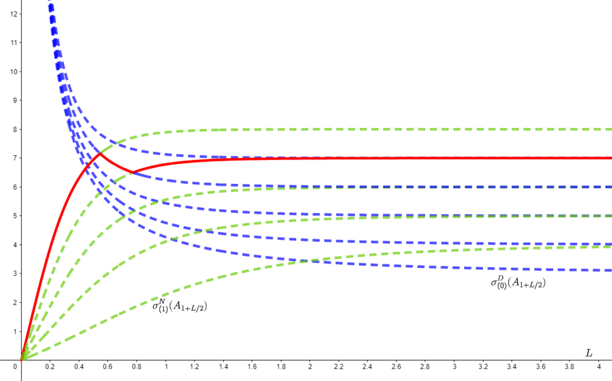
Figure 1. Representation of the case $n=5$. The decreasing blue curves represent $L\longmapsto\sigma_{(i)}^{D}(A_{1+L/2})$ for $i=0,\ldots,4$ while the increasing green curves represent $L\longmapsto\sigma_{(i)}^{N}(A_{1+L/2})$ for $i=1\ldots,5$. The solid red curve is the sharp upper bound $B_{5}^{127}(L)$ that we obtain thanks to the extension process.

Let us prove that $B_{n}^{k}(L)$ is indeed the bound that we were looking for.

Proof of Theorem 4.

We will use the same strategy that was already used in the proof of [10, Theorem 3]. Let us start by showing that $\sigma_{k}(M,g)<B_{n}^{k}(L)$.

Since $\nu_{l_{1}}$ has multiplicity $\mu_{l_{1}}$, there exist $\mu_{l_{1}}$ independent eigenfunctions $\xi_{1},\ldots,\xi_{\mu_{l_{1}}}$ associated with $\nu_{l_{1}}$.

Now we consider the function

$$\xi_{\mu_{l_{1}}}:[0,\frac{L}{2}]\times\mathbb{S}^{n-1}\longrightarrow\mathbb{R},$$

and look at two cases:

1. Let us suppose that $\xi_{\mu_{l_{1}}}$ is a Steklov-Dirichlet eigenfunction. Then $\xi_{\mu_{l_{1}}}(L/2)=0$ and we can extend $\xi_{\mu_{l_{1}}}$ to a new function

   $$\tilde{\xi}_{\mu_{l_{1}}}:[0,L]\times\mathbb{S}^{n-1} \longrightarrow\mathbb{R}$$

   $$(r,p) \longmapsto\left\{\begin{array}[]{cc}\xi_{\mu_{l_{1}}}(r,p)&\mbox{ if }0\leq r\leq L/2\\ -\xi_{\mu_{l_{1}}}(L-r,p)&\mbox{ if }L/2\leq r\leq L.\end{array}\right.$$

   The function $\tilde{\xi}_{\mu_{l_{1}}}$ is continuous. Let us call $f_{0}=u_{0}S_{0},\;f_{1}=u_{1}S_{1},\ldots,\;f_{k-1}=u_{k-1}S_{k-1}$ some Steklov eigenfunctions associated with the $k$ first Steklov eigenvalues $\sigma_{0}(M,g)=0,\;\sigma_{1}(M,g),\ldots,\;\sigma_{k-1}(M,g)$ respectively. Then, since $\xi_{\mu_{l_{1}}}$ is a Steklov-Dirichlet eigenfunction and

   $$\sum_{i=0}^{l_{1}}\mu_{i}\geq k,$$

   we have $\tilde{\xi}_{\mu_{l_{1}}}=\alpha_{l}S_{l}$, for some $l\geq k-1$. Then

   $$\int_{\Sigma}f_{i}\tilde{\xi}_{\mu_{l_{1}}}dV_{\Sigma}=0\;\mbox{ for all }\;i=0,\ldots,k-1.$$

2. Let us suppose that $\xi_{\mu_{l_{1}}}$ is a Steklov-Neumann eigenfunction. Then we can extend $\xi_{\mu_{l_{1}}}$ to a new function

   $$\tilde{\xi}_{\mu_{l_{1}}}:[0,L]\times\mathbb{S}^{n-1} \longrightarrow\mathbb{R}$$

   $$(r,p) \longmapsto\left\{\begin{array}[]{cc}\xi_{\mu_{l_{1}}}(r,p)&\mbox{ if }0\leq r\leq L/2\\ \xi_{\mu_{l_{1}}}(L-r,p)&\mbox{ if }L/2\leq r\leq L.\end{array}\right.$$

   The function $\tilde{\xi}_{\mu_{l_{1}}}$ is continuous. Let us call $f_{0}=u_{0}S_{0},\;f_{1}=u_{1}S_{1},\ldots,\;f_{k-1}=u_{k-1}S_{k-1}$ some Steklov eigenfunctions associated with the $k$ first Steklov eigenvalues $\sigma_{0}(M,g)=0,\;\sigma_{1}(M,g),\ldots,\;\sigma_{k-1}(M,g)$ respectively. Then, since $\xi_{\mu_{l_{1}}}$ is a Steklov-Neumann eigenfunction and

   $$\sum_{i=0}^{l_{1}}\mu_{i}\geq k,$$

   we have $\tilde{\xi}_{\mu_{l_{1}}}=\beta_{l}S_{l}$, with $l\geq k$. Then

   $$\int_{\Sigma}f_{i}\tilde{\xi}_{\mu_{l_{1}}}dV_{\Sigma}=0\;\mbox{ for all }\;i=0,\ldots,k-1.$$

Therefore, in both cases we have $\int_{\Sigma}f_{i}\tilde{\xi}_{\mu_{l_{1}}}dV_{\Sigma}=0$ for all $i=0,\ldots,k-1$. Hence we can use $\tilde{\xi}_{\mu_{l_{1}}}$ as a test function for $\sigma_{k}(M,g)$, thanks to Equation 1. We get

$$\sigma_{k}(M,g) \leq R_{g}(\tilde{\xi}_{\mu_{l_{1}}})$$

$$<R_{\tilde{g}}(\tilde{\xi}_{\mu_{l_{1}}})\quad\mbox{ where }\tilde{g}=dr^{2}+\tilde{h}^{2}g_{0}\mbox{ comes from \cite[cite]{[\@@bibref{}{T_revolution}{}{}, Theorem 2]} }$$

$$=\frac{\int_{0}^{L}\int_{\mathbb{S}^{n-1}}\left((\partial_{r}\tilde{\xi}_{\mu_{l_{1}}})^{2}+\frac{1}{\tilde{h}(r)^{2}}|\tilde{\nabla}\tilde{\xi}_{\mu_{l_{1}}}|^{2}\right)\tilde{h}(r)^{n-1}dV_{g_{0}}dr}{\int_{\Sigma}\tilde{\xi}_{\mu_{l_{1}}}^{2}(0,p)dV_{\Sigma}}$$

$$=\frac{2\times\int_{0}^{L/2}\int_{\mathbb{S}^{n-1}}\left((\partial_{r}\tilde{\xi}_{\mu_{l_{1}}})^{2}+\frac{1}{\tilde{h}(r)^{2}}|\tilde{\nabla}\tilde{\xi}_{\mu_{l_{1}}}|^{2}\right)\tilde{h}(r)^{n-1}dV_{g_{0}}dr}{2\times\int_{\mathbb{S}^{n-1}}\tilde{\xi}_{\mu_{l_{1}}}^{2}(0,p)dV_{g_{0}}}\quad(\tilde{g}\mbox{ is symmetric})$$

$$=\frac{\int_{0}^{L/2}\int_{\mathbb{S}^{n-1}}\left((\partial_{r}\xi_{\mu_{l_{1}}})^{2}+\frac{1}{\tilde{h}(r)^{2}}|\tilde{\nabla}\xi_{\mu_{l_{1}}}|^{2}\right)\tilde{h}(r)^{n-1}dV_{g_{0}}dr}{\int_{\mathbb{S}^{n-1}}\xi_{\mu_{l_{1}}}^{2}(0,p)dV_{g_{0}}}$$

$$<\frac{\int_{0}^{L/2}\int_{\mathbb{S}^{n-1}}\left((\partial_{r}\xi_{\mu_{l_{1}}})^{2}+\frac{1}{(1+r)^{2}}|\tilde{\nabla}\xi_{\mu_{l_{1}}}|^{2}\right)(1+r)^{n-1}dV_{g_{0}}dr}{\int_{\mathbb{S}^{n-1}}\xi_{\mu_{l_{1}}}^{2}(0,p)dV_{g_{0}}}$$

$$=\nu_{l_{1}}$$

$$=B_{n}^{k}(L),$$

where the second strict inequality comes from the existence of a continuum of points $r\in[0,L/2]$ such that $\tilde{h}(r)<1+r$.

We still have to show that the upper bound $B_{n}^{k}(L)$ is sharp, i.e for all $\varepsilon>0$, there exists a metric of revolution $g_{\varepsilon}$ on $M$ such that

$$\sigma_{k}(M,g_{\varepsilon})>B_{n}^{k}(L)-\varepsilon.$$

Let $\varepsilon>0$. Let $M=[0,L]\times\mathbb{S}^{n-1}$ and let $g_{\varepsilon}(r,p)=dr^{2}+h_{\varepsilon}^{2}(r)g_{0}(p)$ be a metric of revolution on $M$ such that

1. For all $r\in[0,L]$, we have $h_{\varepsilon}(r)=h_{\varepsilon}(L-r)$ (i.e $h_{\varepsilon}$ is symmetric).

2. For all $r\in[0,L/2-\delta]$, we have $h_{\varepsilon}(r)=(1+r)$, with $\delta$ small enough to guarantee that for all $r\in[0,L/2]$, we have $\max\{(1+r)^{n-3}-h_{\varepsilon}(r)^{n-3},(1+r)^{n-1}-h_{\varepsilon}(r)^{n-1}\}<\frac{\varepsilon}{B_{n}^{k}(L)}=:\varepsilon^{*}$.

We write $f_{k}$ a Steklov eigenfunction associated with $\sigma_{k}(M,g_{\varepsilon})$. Because $g_{\varepsilon}$ is symmetric, we can choose $f_{k}$ symmetric or anti-symmetric. Writing

$$R_{A_{1+L/2}}(f_{k}):=\frac{\int_{0}^{{L}/2}\int_{\mathbb{S}^{n-1}}\left((\partial_{r}f_{k})^{2}+\frac{1}{(1+r)^{2}}|\tilde{\nabla}f_{k}|^{2}\right)(1+r)^{n-1}dV_{g_{0}}dr}{\int_{\mathbb{S}^{n-1}}(f_{k})^{2}(0,p)dV_{g_{0}}},$$

it is an easy computation to check that

$$R_{A_{1+L/2}}(f_{k})<\sigma_{k}(M,g_{\varepsilon})+\varepsilon.$$

We once again split the proof into two cases:

1. Let us suppose that $f_{k}$ is anti-symmetric, i.e we have $f_{k}(r,p)=u_{k}(r)S_{l}(p)$ with $u_{k}$ anti-symmetric and $B_{n}^{k}(L)=\sigma_{j}^{D}(A_{1+L/2})$ for a certain $j\leq l$. Then we can check that

   $$f_{k}(L/2,p)=0\mbox{ and }\int_{\{0\}\times\mathbb{S}^{n-1}}\varphi_{i}f_{k}dV_{g_{0}}=0\mbox{ for all }i=0,\ldots,l-1.$$

2. Let us suppose that $f_{k}$ is symmetric, i.e we have $f_{k}(r,p)=u_{k}(r)S_{l}(p)$ with $u_{k}$ symmetric and $B_{n}^{k}(L)=\sigma_{j}^{N}(A_{1+L/2})$ for a certain $j\leq l$. Then we can check that

   $$\partial_{r}f_{k}(L/2,p)=0\mbox{ and }\int_{\{0\}\times\mathbb{S}^{n-1}}\phi_{i}f_{k}dV_{g_{0}}=0\mbox{ for all }i=0,\ldots,l-1.$$

In both cases, we can use $f_{k}|_{[0,L/2]\times\mathbb{S}^{n-1}}$ as a test function for $B_{n}^{k}(L)$, and we get

$$B_{n}^{k}(L)<R_{A_{1+L/2}}(f_{k})<\sigma_{k}(M,g_{\varepsilon})+\varepsilon.$$

∎

From this statement, let us prove Corollary 5.

Proof.

Let $k\geq 1$. We want to show the existence of a bound $B_{n}^{k}<\infty$ such that for all hypersurfaces of revolution $(M,g)$ of dimension $n\geq 3$, we have $\sigma_{k}(M,g)<B_{n}^{k}$. A way to do it is the analyse to function $L\longmapsto B_{n}^{k}(L)$, and defining $B_{n}^{k}$ as follows:

$$B_{n}^{k}:=\sup\{B_{n}^{k}(L):L\in\mathbb{R}_{+}^{*}\}.$$

By construction, we have $\sigma_{k}(M,g)<B_{n}^{k}$. We only have to show that $B_{n}^{k}$ is finite. Indeed, for all $L\in\mathbb{R}_{+}^{*}$, we have

$$B_{n}^{k}(L)<\sigma_{(k)}^{N}(L).$$

Therefore, we have

$$B_{n}^{k} =\sup\{B_{n}^{k}(L):L\in\mathbb{R}_{+}^{*}\}$$

$$\leq\sup\{\sigma_{(k)}^{N}(A_{1+L/2}):L\in\mathbb{R}_{+}^{*}\}$$

$$=\lim_{L\to\infty}\sigma_{(k)}^{N}(A_{1+L/2})$$

$$=n+k-2.$$

Now we can prove that $B_{n}^{k}$ is a sharp upper bound, that is for all $\varepsilon>0$, there exists a hypersurface of revolution $(M_{\varepsilon},g_{\varepsilon})$ such that $\sigma_{k}(M_{\varepsilon},g_{\varepsilon})>B_{n}^{k}-\varepsilon$.

Let $\varepsilon>0$. There exists $L^{*}\in\mathbb{R}_{+}^{*}$ such that $B_{n}^{k}-B_{n}^{k}(L^{*})<\frac{\varepsilon}{2}$. We define $M_{\varepsilon}:=[0,L^{*}]\times\mathbb{S}^{n-1}$. Thanks to Theorem 4, there exists a metric of revolution $g_{\varepsilon}$ on $M_{\varepsilon}$ such that

$$\sigma_{k}(M_{\varepsilon},g_{\varepsilon})>B_{n}^{k}(L^{*})-\frac{\varepsilon}{2}>B_{n}^{k}-\frac{\varepsilon}{2}-\frac{\varepsilon}{2}=B_{n}^{k}-\varepsilon.$$

∎

From Theorem 4, let us prove Corollary 6.

Proof.

Let us notice that given $j\in\mathbb{N}$ fixed, we have

$$\lim_{L\to 0}\sigma_{(j)}^{D}(A_{1+L/2})=\infty\quad\mbox{ and }\quad\lim_{L\to 0}\sigma_{(j)}^{N}(A_{1+L/2})=0.$$

Let $k\in\mathbb{N}$ and let $\varepsilon>0$. Let $L_{0}>0$ be small enough so that $\sigma_{(1)}^{N}(A_{1+L_{0}/2})<\ldots<\sigma_{(k)}^{N}(A_{1+L_{0}/2})<\varepsilon$. Let $0<L<L_{0}$. Then the finite set $E=E(n,k,L)$ can be ordered and $\nu_{0},\ldots,\nu_{l_{0}+1}$ are equal respectively to $\sigma_{(1)}^{N}(A_{1+L/2}),\ldots,\sigma_{(l_{0}+1)}^{N}(A_{1+L/2})$, where $l_{0}+1<k$.

Hence $\nu_{l_{1}}\in\{\sigma_{(1)}^{N}(A_{1+L/2}),\ldots,\sigma_{(l_{0}+1)}^{N}(A_{1+L/2})\}$ and therefore, writing $M:=[0,L]\times\mathbb{S}^{n-1}$,

$$\sigma_{k}(M,g)<\nu_{l_{1}}\leq\max\{\sigma_{(1)}^{N}(A_{1+L/2}),\ldots,\sigma_{(l_{0}+1)}^{N}(A_{1+L/2})\}<\varepsilon.$$

∎

4. Question and conjecture

We now investigate if the sharp upper bound $B_{n}^{k}$ is achieved by a finite critical length $L_{k}$ or an infinite one. In particular, we are interested to know if the infinite critical length happens only finitely often. As the question is complex, we used a program that, given a dimension $n$ and an integer $k$, checks if the eigenvalues with index smaller or equal to $k$ have finite or infinite critical length. The code for this program is given in Appendix C.

Such a program requires quite some computation time to run, at least if we want to check many eigenvalues. Here are some considerations used in order to optimize the program.

Definition 16.

Given a dimension $n\geq 3$, we say that $k\in\mathbb{N}$ is a diagnosis eigenvalue if $k=\sum_{j=0}^{i-1}2m_{j}$ for a certain integer $i$.

This definition is motivated by the following lemma:

Lemma 17.

Let $n\geq 3$ and $i\in\mathbb{N}$. Let $k:=\sum_{j=0}^{i-1}2m_{j}$ be the $i$th diagnosis eigenvalue. Let us suppose that $k$ has an associated finite critical length. Then, for each $k^{\prime}\in\{k,\dots,k+2m_{i}-1\}$, the eigenvalue $k^{\prime}$ has an associated finite critical length.

Proof.

Since $k=\sum_{j=0}^{i-1}2m_{j}$, there exists $C>0$ such that $B_{n}^{k}(L)=\sigma_{(i)}^{N}(A_{1+L/2})$ for all $L>C$. Moreover, since $L\longmapsto\sigma_{(i)}^{N}(A_{1+L/2})$ is strictly increasing, then the critical length $L_{k}$ (which is finite by assumption) satisfies $L_{k}\leq C$.

Let us fix $L^{*}>C$. Then for each $k^{\prime}$ such that $k\leq k^{\prime}<k+m_{i}$, we have $B_{n}^{k^{\prime}}(L^{*})=\sigma_{(i)}^{N}(A_{1+L^{*}/2})$. Moreover, we have $B_{n}^{k^{\prime}}(L_{k})\geq B_{n}^{k}(L_{k})$. Thus, we have

$$\sigma_{(i)}^{N}(A_{1+L^{*}/2})<B_{n}^{k}(L_{k})\leq B_{n}^{k^{\prime}}(L_{k})\leq\sup_{L\in(0,C]}B_{n}^{k^{\prime}}(L),$$

and $k^{\prime}$ has a finite critical length.

Finally, for $k^{\prime}$ such that

$$k+m_{i}\leq k^{\prime}<k+2m_{i},$$

we have $B_{n}^{k^{\prime}}(L)=\sigma_{(i)}^{D}(A_{1+L/2})$ for all $L>C$. Moreover, since $L\longmapsto\sigma_{(i)}^{D}(A_{1+L/2})$ is decreasing, we know that $k^{\prime}$ has a finite critical length.

Therefore, for all $k^{\prime}\in\{k,\dots,k+2m_{i}-1\}$, the eigenvalue $k^{\prime}$ has an associated finite critical length.

∎

Example 18.

Let $n=5$. The sequence of diagnosis eigenvalues is

$$(2,12,40,100,210,392,672,1^{\prime}080,1^{\prime}650,2^{\prime}420,3^{\prime}432,4^{\prime}732,6^{\prime}370,8^{\prime}400,10^{\prime}880,\ldots).$$

The lemma allows us to state that in dimension $5$, if the $14$th diagnosis eigenvalue $k=8^{\prime}400$ has an associated finite critical length, then for each $k^{\prime}\in\{8^{\prime}400,\dots,10^{\prime}879\}$, the $k^{\prime}$th eigenvalue has an associated finite critical length.

Therefore, it is relevant to consider only these diagnosis eigenvalues to save time while checking what could be the answer to our open question.

Here are some of the results obtained by our program:

$$\begin{array}[]{ccl}n&i&\mbox{Result of the program's investigations}\\ \hline\cr 3&150&\mbox{From $k=18$ to $k=45^{\prime}601$, only finite critical lengths found.}\\ 4&40&\mbox{From $k=408$ to $k=47^{\prime}641$, only finite critical lengths found.}\\ 5&30&\mbox{From $k=8^{\prime}400$ to $k=195^{\prime}423$, only finite critical lengths found.}\\ 6&25&\mbox{From $k=21^{\prime}112$ to $k=610^{\prime}973$, only finite critical lengths found.}\end{array}$$

We draw attention to the fact that the program does not say that in dimension $3$, the eigenvalue number $17$ has a critical length at infinity, it only says that it has not found any infinite critical length above $17$. Actually, in dimension $n=3$, we have not found any infinite critical length associated with the eigenvalue $k$, if $k>8$.

These numerical results motivate 8:

Let $n\geq 3$ be an integer. Then there exists $K=K(n)\in\mathbb{N}$ such that for every $k\geq K$, the $k$th eigenvalue has an associated finite critical length.

If this conjecture were to be proven, it would then be interesting to study the function

$$n\longmapsto K_{min}(n),$$

where $K_{min}(n)$ is the smallest integer in the conjecture. From our numerical experiments, it seems that this function, if it exists, grows quickly with $n$.

5. Proof of the conjecture in low dimension

Notation. If the context is clear, we write $\sigma_{(\kappa)}^{D/N}(L)$ instead of $\sigma_{(\kappa)}^{D/N}(A_{1+L/2})$ to streamline the notations.

The goal of this section is to prove 9. The idea of the proof is simple: as explained in previous sections, the bound $B_{n}^{k}(L)$ can be obtained by looking at Steklov-Neumann $\sigma^{N}$ and Steklov-Dirichlet $\sigma^{D}$ eigenvalues on an annulus. So suppose that for a given $k$, the bound $B_{n}^{k}(L)$ is achieved by some $\sigma_{(\kappa)}^{N}(L)$ for $L$ near 0. We know the curve $L\mapsto\sigma_{(\kappa)}^{N}(L)$ will intersect the curves of $\sigma_{(0)}^{D}(L),\sigma_{(1)}^{D}(L),\dots,\sigma_{(\kappa-1)}^{D}(L)$. Hence looking at the multiplicities carried by each curve, one can see that for large enough $L$, the bound $B_{n}^{k}(L)$ cannot continue to be achieved by $\sigma_{(\kappa)}^{N}(L)$ and must be achieved by a lower curve. Applying this reasoning to more curves $\sigma^{N}(L)$, we will obtain an upper bound on the index of the curve $\sigma^{N}$ which can be achieved for large $L$ (c.f. Lemma 21). This allows us to obtain an upper bound for $B_{n}^{k}(L)$ when $L\to\infty$. Meanwhile, looking at the intersection of $\sigma_{(\kappa)}^{N}(L)$ and $\sigma_{(0)}^{D}(L)$, we obtain a lower bound for $B_{k}^{n}$ (Lemma 19). In dimensions $n=3$ or $n=4$, this bound is bigger than the one achieved at infinity allowing us to conclude that we must have a finite critical length.

We recall that the multiplicity $m_{k}$ of the eigenvalue $\sigma_{(k)}^{N/D}(A_{1+L/2})$ is given by

$$m_{k} =\frac{(n+k-3)!}{(n-2)!k!}(n+2k-2)$$

$$=\frac{(k+n-3)(k+n-4)\dots(k+2)(k+1)}{(n-2)!}(2k+n-2).$$

We first prove the following lemma:

Lemma 19.

Let $n\in\mathbb{N}$. For $\kappa\in\mathbb{N}$, let $b_{\kappa}\in\mathbb{R}$ be the value such that

$$\sigma_{(\kappa)}^{N}(A_{1+L/2})=b_{\kappa}=\sigma_{0}^{D}(A_{1+L/2}).$$

Let $c_{0}\approx 0.83$ be the unique positive solution of the equation $\frac{1+c}{1-c}=e^{2/c}$. Then for any $0<c<c_{0}$, there exists $\kappa_{0}(c)$ such that for all $\kappa\geq\kappa_{0}$,

$$b_{\kappa}\geq c\kappa.$$

Proof.

Since $\sigma_{0}^{D}$ and $\sigma_{(\kappa)}^{N}$ are monotone in $L$, we can invert them and give an expression for $(\sigma_{0}^{D})^{-1}$ and $(\sigma_{(\kappa)}^{N})^{-1}$. We get

$$(\sigma^{D}_{0})^{-1}(y)=\left(1+\frac{n-2}{y-(n-2)}\right)^{\frac{1}{n-2}}$$

and

$$(\sigma^{N}_{(\kappa)})^{-1}(y)=\left(\frac{1+\frac{y}{\kappa}}{1-\frac{y}{\kappa+n-2}}\right)^{\frac{1}{2\kappa+n-2}}.$$

With the notation $y_{\kappa}=c\kappa$, we have to show that

$$(\sigma^{N}_{(\kappa)})^{-1}(y_{\kappa})\leq(\sigma^{D}_{0})^{-1}(y_{\kappa})$$

if $\kappa$ is large enough. Here we use that $\sigma^{N}(\kappa)$ is increasing and $\sigma^{D}_{0}$ is decreasing.

Therefore, we need to show that for large enough $\kappa$, we have

$$\frac{1+\frac{y_{\kappa}}{\kappa}}{1-\frac{y_{\kappa}}{\kappa+n-2}}\leq\left(1+\frac{n-2}{y_{\kappa}-(n-2)}\right)^{\frac{2\kappa+n-2}{n-2}}.$$

We have for the left-hand-side

$$\frac{1+\frac{c\kappa}{\kappa}}{1-\frac{c\kappa}{\kappa+n-2}}=\frac{1+c}{1-c}+\mathcal{O}(\frac{1}{\kappa}),$$

and for the right-hand-side

$$\left(1+\frac{n-2}{c\kappa-(n-2)}\right)^{\frac{2\kappa+n-2}{n-2}} =e^{\frac{2\kappa+n-2}{n-2}\log\left(1+\frac{n-2}{c\kappa-(n-2)}\right)}$$

$$=e^{\frac{2\kappa+n-2}{n-2}\left(\frac{n-2}{c\kappa-(n-2)}+\mathcal{O}(\frac{1}{\kappa^{2}})\right)}$$

$$=e^{\frac{2}{c}+\mathcal{O}(\frac{1}{\kappa})}$$

$$=e^{\frac{2}{c}}+\mathcal{O}(\frac{1}{\kappa}).$$

Therefore, we have

$$\lim_{\kappa\to\infty}\frac{1+\frac{c\kappa}{\kappa}}{1-\frac{c\kappa}{\kappa+n-2}}=\frac{1+c}{1-c}<e^{\frac{2}{c}}=\lim_{\kappa\to\infty}\left(1+\frac{n-2}{c\kappa-(n-2)}\right)^{\frac{2\kappa+n-2}{n-2}},$$

since we assumed $0<c<c_{0}$.

∎

Remark 20.

This lemma holds whatever the dimension $n\geq 3$. Moreover, the value of $c_{0}\approx 0.83$ is independent of the dimension.

Lemma 21.

Let $c_{0}\approx 0.83$ be the unique positive solution of the equation $\frac{1+c}{1-c}=e^{2/c}$. For $n=3$ or $n=4$, there exists $\kappa_{1}\in\mathbb{N}$ such that for all $\kappa\geq\kappa_{1}$,

$$m_{\kappa}+m_{\kappa-1}+\dots+m_{\lfloor c_{0}\kappa\rfloor}<m_{0}+m_{1}+\dots+m_{\lfloor c_{0}\kappa\rfloor-1}.$$

Proof.

Let us suppose $n=3$. Then we have $m_{i}=2i+1$, therefore

$$m_{0}+m_{1}+\ldots+m_{\kappa}=1+3+\ldots+(2\kappa+1)=(\kappa+1)^{2},$$

and

$$m_{0}+m_{1}+\ldots+m_{\lfloor c_{0}\kappa\rfloor-1}=\lfloor c_{0}\kappa\rfloor^{2}.$$

Hence, we have

$$\frac{m_{0}+\ldots+m_{\kappa}}{m_{0}+m_{1}+\ldots+m_{\lfloor c_{0}\kappa\rfloor-1}}=\frac{(\kappa+1)^{2}}{\lfloor c_{0}\kappa\rfloor^{2}}\underset{\kappa\to\infty}{\longrightarrow}\frac{1}{c_{0}^{2}}<2.$$

Therefore, there exists $\kappa_{1}\in\mathbb{N}$ such that for all $\kappa\geq\kappa_{1}$, we have

$$m_{\kappa}+m_{\kappa-1}+\dots+m_{\lfloor c_{0}\kappa\rfloor}<m_{0}+m_{1}+\dots+m_{\lfloor c_{0}\kappa\rfloor-1}.$$

Let us suppose $n=4$. Then we have $m_{i}=(i+1)^{2}$, therefore

$$m_{0}+m_{1}+\ldots+m_{\kappa}=\frac{(\kappa+1)(\kappa+2)(2\kappa+3)}{6}$$

and

$$m_{0}+m_{1}+\ldots+m_{\lfloor c_{0}\kappa\rfloor-1}=\frac{\lfloor c_{0}\kappa\rfloor(\lfloor c_{0}\kappa\rfloor+1)(2\lfloor c_{0}\kappa\rfloor+1)}{6}.$$

Hence, we have

$$\frac{m_{0}+m_{1}+\ldots+m_{\kappa}}{m_{0}+m_{1}+\ldots+m_{\lfloor c_{0}\kappa\rfloor-1}}\underset{\kappa\to\infty}{\longrightarrow}\frac{1}{c_{0}^{3}}<2.$$

Therefore, there exists $\kappa_{1}\in\mathbb{N}$ such that for all $\kappa\geq\kappa_{1}$, we have

$$m_{K}+m_{\kappa-1}+\dots+m_{\lfloor c_{0}\kappa\rfloor}<m_{0}+m_{1}+\dots+m_{\lfloor c_{0}\kappa\rfloor-1}.$$

∎

Remark 22.

In dimension $n\geq 5$, the previous lemma does not hold. Indeed, one can see that $m_{i}$ is polynomial of degree $(n-2)$, $m_{i}=\frac{2i^{n-2}}{(n-2)!}+\mathcal{O}(i^{n-3})$. Hence, if we search for the best $c$ such that the lemma hold, we must solve for $c$ and in the limit $\kappa\to\infty$, the equation

$$\frac{2\kappa^{n-1}}{(n-1)(n-2)!}+\mathcal{O}(\kappa^{n-2})=\sum_{i=0}^{\kappa}m_{i}=\sum_{i=0}^{c\kappa}m_{i}=\frac{2(c\kappa)^{n-1}}{(n-1)(n-2)!}+\mathcal{O}(\kappa^{n-2}).$$

This gives $c=\left(\frac{1}{2}\right)^{\frac{1}{n}}$. As $n\to\infty$, $c\to 1$ and in fact for $n\geq 5$, $c>c_{0}$.

Lemma 23.

For $n\in\{3,4\}$, there exists a $K_{3}\in\mathbb{N}$ such that for any $k\geq K_{3}$, we have

$$B_{n}^{k}=\sup_{L\in(0,\infty)}\{B_{n}^{k}(L)\}>\lim_{L\to\infty}B_{n}^{k}(L).$$

Proof.

Let $n\in\{3,4\}$. Let $\kappa\geq K_{3}:=\max\{\kappa_{0},\kappa_{1}\}$, where $\kappa_{0}$ and $\kappa_{1}$ are as in the preceding lemmas. Let $k$ be such that

$$m_{0}+m_{1}+\ldots+m_{\kappa-1}<k\leq m_{0}+m_{1}+\ldots m_{\kappa}.$$

Then, for $L$ small enough, we have

$$B_{n}^{k}(L)=\sigma_{\kappa}^{N}(A_{1+L/2}).$$

Moreover,

$$k\leq m_{0}+\ldots+m_{\lfloor 0.8\kappa\rfloor-1}+m_{\lfloor 0.8\kappa\rfloor}+\ldots+m_{\kappa}\stackrel{{\scriptstyle\lx@cref{creftypecap~refnum}{lem : tech 2}}}{{<}}2\cdot\left(m_{0}+\ldots+m_{\lfloor 0.8\kappa\rfloor-1}\right).$$

Therefore, for $L$ large enough, we have

$$B_{n}^{k}(L)\leq\sigma_{\lfloor 0.8\kappa\rfloor-1}^{N}(A_{1+L/2})\underset{L\to\infty}{\longrightarrow}\lfloor 0.8\kappa\rfloor+n-3,$$

as shown in Figure 2.

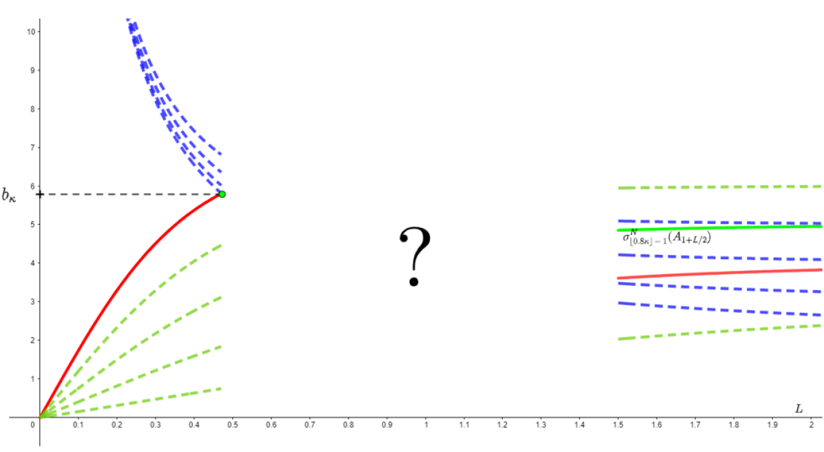
Figure 2. Before the intersections (the region covered by the interrogation mark), the sharp upper bound is given by $\sigma_{(\kappa)}^{N}(A_{1+L/2})$ and after, an upper bound (non necessarily sharp) is given by $\sigma_{(\lfloor 0.8\kappa\rfloor-1)}^{N}(A_{1+L/2})$, which is lower than $b_{\kappa}$.

Moreover, Lemma 19 allows us to state that $b_{\kappa}\geq c_{0}\kappa>\lfloor 0.8\kappa\rfloor+n-3$ because $\kappa$ is large enough. Therefore,

$$B_{n}^{k}\geq b_{\kappa}\geq c_{0}\kappa>\lfloor 0.8\kappa\rfloor+n-3,$$

and hence

$$B_{n}^{k}=B_{n}^{k}(L_{k})$$

for a certain $L_{k}$ finite, which means that $k$ has a finite critical length.

∎

Appendix A Plotting sharp upper bounds

We can implement the extension process in a computer and let the value of $L$ vary in order to plot the sharp upper bound as a function of $L$, where we see $n$ and $k$ as parameters.

Here are some figures obtained. On the bottom-right part of each graphic, one can see written "$B_{n}^{k}$", meaning that we studied the $n$th dimension and the $k$th eigenvalue. Moreover, for each values of $n$ and $k$, the graphic indicates if we found a finite or infinite critical length, and provides an estimation of the critical length as well as an estimation of the sharp upper bound $B_{n}^{k}$.

Figure 3. As one can see, the behaviour of the function $L\longmapsto B_{n}^{k}(L)$ is hard to predict, and its properties (smoothness, infinite critical length, finite critical length) depend on the values of $n$ and $k$.

Appendix B Adding the mixed eigenvalues

Since the function $L\longmapsto B_{n}^{k}(L)$ comes from the mixed Steklov-Dirichlet and Steklov-Neumann eigenvalues, we can add them in the graphics to understand the function better.

We got the following figures.

Figure 4. The blue curves are the Steklov-Dirichlet eigenvalues, the green ones are the Steklov-Neumann eigenvalues.

Appendix C Python codes

The codes that are provided here can also be found on Github, with some other documents (such as results, time of computation, etc.), at the address:

https://github.com/Tchatchu5

C.1. Functions

We code for some functions that are used in the extension process.

⬇

1import functools

2

3from math import factorial

4

5# function multiplicity of the Laplace eigenvalues on a sphere

6@functools.cache

7def mu(n, k):

8 return int((n + 2 * k - 2) * factorial(n + k - 3) /

9 (factorial(k) * factorial(n - 2)))

10

11

12# Steklov - Dirichlet eigenvalue on an annulus

13def sigma_dirichlet(n, D, L):

14 if L == 0:

15 return float("inf")

16 return ((n + D - 2) * (1 + L / 2)**(2 * D + n - 2) + D) / \

17 ((1 + L / 2)**(2 * D + n - 2) - 1)

18

19

20# Steklov - Neumann eigenvalue on an annulus

21def sigma_neumann(n, N, L):

22 return N * ((N + n - 2) * ((1 + L / 2)**(2 * N + n - 2) - 1)) / \

23 (N * (1 + L / 2)**(2 * N + n - 2) + N + n - 2)

24

25

26# function which return the integer l_0 in the extension process

27@functools.cache

28def l_0(n, k):

29 list = []

30 for i in range(0, k + 1):

31 list.append((mu(n, i)))

32 sum = 0

33 j = 0

34 for i in range(0, k + 1):

35 if sum + list[i] > k:

36 return j

37 sum = sum + list[i]

38 j = j + 1

39 return None

40

41

42# function which return the integer l_1 in the extension process

43def l_1(m2_list: list, k: int) -> int:

44 """Compute the L_1 number representing the number of incremental addition to perform from M2’s list values in order to

45 go above or equal to K

46 Args

47 ----

48 * m2_list: list of M sorted according to its respective value in E

49 * K: Knt eigenvalue

50 Returns

51 ----

52 The number of additions performed

53 """

54 i, accumulator = 0, 0

55 while accumulator < k:

56 accumulator += m2_list[i]

57 i += 1

58 # Reverse latest addition that brought us above K

59 return i - 1

60

61

62# function which gives the sharp upper bound in the extension process

63def sharp_upper_bound(n, k, L):

64 E = []

65 for i in range(0, l_0(n, k) + 1):

66 E.append(sigma_dirichlet(n, i, L))

67 for i in range(1, l_0(n, k) + 2):

68 E.append(sigma_neumann(n, i, L))

69

70 M = []

71 for i in range(0, l_0(n, k) + 1):

72 M.append(mu(n, i))

73 for i in range(1, l_0(n, k) + 2):

74 M.append(mu(n, i))

75

76 #print(f"Before, e:{E}\nm:{M}")

77 link_dict = {}

78 for i in range(len(E)):

79 key = E[i]

80 value = M[i]

81 try:

82 link_dict[key].append(value)

83 except KeyError as e:

84 link_dict[key] = [value]

85

86 #print(f"Link dict: {link_dict}")

87 E.sort()

88 M2 = [link_dict[e_value].pop(0) for e_value in E]

89

90 l1 = l_1(M2, k)

91

92 #print(f"sorted E: {E}\nSorted M2:{M2}")

93 #print(f"Computing addition number to obtain a value >= K")

94 return E[l1]

95 #print(f"From list: {M2}, There need to be {l1} addition to obtain accumulator >= K = {k}")

96 #print(f"From list {E}, at index {l1} = {E[l1]}")

C.2. Sharp upper bound

Here is a first program which takes three inputs (the dimension $n$, the $k$th eigenvalue and the meridian length $L$) and gives as output the sharp upper bound $B_{n}^{k}(L)$.

⬇

1import functions

2

3

4n=int(input("Which dimension do you want to study?"))

5k=int(input("Which eigenvalue do you want to study?"))

6L=float(input("Which meridian length o you want to study?"))

7

8print(f"The sharp upper bound for the {k}th Steklov eigenavlue of a hypersurface of revolution in the Euclidean space, with meridian length {L} and dimension {n} is {functions.sharp_upper_bound(n, k, L)}")

C.3. Plot sharp upper bound

Now we code for a program that takes the dimension $n$ and the $k$th eigenvalue $k$ as inputs, and produces a plot of the function

$$\mathbb{R}_{+}^{*} \longrightarrow\mathbb{R}$$

$$L \longmapsto B_{n}^{k}(L).$$

⬇

1import matplotlib.pyplot as plt

2import numpy as np

3

4import functions

5

6n = int(input("Which dimension do you want to study?"))

7k = int(input("Which eigenvalue do you want to study?"))

8

9# first interval that we want to study

10X = np.linspace(0, 7, max(400, k**2))

11# for each value of L, find the sharp upper bound depending on n, k, L

12Y = []

13for l in X:

14 Y.append(functions.sharp_upper_bound(n, k, l))

15# find the critical length

16y_max_index = Y.index(max(Y))

17if max(Y) > Y[-1]:

18 critical_length = round(X[y_max_index], 3)

19else:

20 critical_length = "infinite"

21

22# refine the interval according to the critical length

23if critical_length == "infinite":

24 pass

25else:

26 X = np.linspace(0, min(critical_length * 4, 7), max(400, k**2))

27 Y = []

28 for l in X:

29 Y.append(functions.sharp_upper_bound(n, k, l))

30 # find the critical length

31 y_max_index = Y.index(max(Y))

32 if max(Y) > Y[-1]:

33 critical_length = round(X[y_max_index], 3)

34 else:

35 critical_length = "infinite"

36

37

38if max(Y) > Y[-1]:

39 critical_length2 = "Finite critical length"

40else:

41 critical_length2 = "Infinite critical length"

42

43# find the sharp upper bound depending on n, k

44if max(Y) > Y[-1]:

45 upper_bound = round(max(Y), 3)

46else:

47 upper_bound = round(max(Y))

48

49# centering the figure

50if critical_length == round(X[y_max_index], 3):

51 center_x = min(critical_length * 4, 7)

52else:

53 center_x = 7

54# plotting the sharp upper bound

55plt.plot(X, Y, "r")

56# lengending according to the indicators found

57plt.title(critical_length2)

58plt.xlabel("Value of L")

59plt.ylabel(f"{k}th eigenvalue")

60plt.figtext(0.6, 0.3, f"Critical length {critical_length}", style="italic")

61plt.figtext(0.6, 0.2, f"B_{n}^{k} = {upper_bound}", style="italic")

62plt.axis([0, center_x, 0, max(Y) + 2])

63plt.show()

C.4. Adding mixed eigenvalues

Because we know that the function $L\longmapsto B_{n}^{k}(L)$ comes from the mixed Steklov-Dirichlet and Steklov-Neumann eigenvalues, we code a program that add them in the previous plots.

⬇

1import matplotlib.pyplot as plt

2import numpy as np

3

4import functions

5

6n = int(input("Which dimension do you want to study?"))

7k = int(input("Which eigenvalue do you want to study?"))

8

9# first interval that we want to study

10X = np.linspace(0, 7, max(400, k ** 2))

11# for each value of L, find the sharp upper bound depending on n, k, L

12Y = []

13for l in X:

14 Y.append(functions.sharp_upper_bound(n, k, l))

15# find the critical length

16y_max_index = Y.index(max(Y))

17if max(Y) > Y[-1]:

18 critical_length = round(X[y_max_index], 3)

19else:

20 critical_length = "infinite"

21

22# refine the interval according to the critical length

23if critical_length == "infinite":

24 pass

25else:

26 X = np.linspace(0, min(critical_length * 4, 7), max(400, k ** 2))

27 Y = []

28 for l in X:

29 Y.append(functions.sharp_upper_bound(n, k, l))

30 # find the critical length

31 y_max_index = Y.index(max(Y))

32 if max(Y) > Y[-1]:

33 critical_length = round(X[y_max_index], 3)

34 else:

35 critical_length = "infinite"

36# endtry

37

38

39if max(Y) > Y[-1]:

40 critical_length2 = "Finite critical length"

41else:

42 critical_length2 = "Infinite critical length"

43

44# find the sharp upper bound depending on n, k

45if max(Y) > Y[-1]:

46 upper_bound = round(max(Y), 3)

47else:

48 upper_bound = round(max(Y))

49

50# plotting Steklov-Dirichlet eigenvalues

51for i in range(0, functions.l_0(n, k) + 1):

52 dirichlet_i = []

53 for l in X:

54 dirichlet_i.append(functions.sigma_dirichlet(n, i, l))

55 plt.plot(X, dirichlet_i, "b")

56# plotting Steklov-Neumann eigenvalues

57for i in range(1, functions.l_0(n, k) + 2):

58 neumann_i = []

59 for l in X:

60 neumann_i.append(functions.sigma_neumann(n, i, l))

61 plt.plot(X, neumann_i, "g")

62# centering the figure

63if critical_length == round(X[y_max_index], 3):

64 center_x = min(critical_length * 4, 7)

65else:

66 center_x = 7

67# plotting the sharp upper bound

68plt.plot(X, Y, "r")

69# lengending according to the indicators found

70plt.title(critical_length2)

71plt.xlabel("Value of L")

72plt.ylabel(f"{k}th eigenvalue")

73plt.figtext(0.6, 0.3, f"Critical length {critical_length}", style="italic")

74plt.figtext(0.6, 0.2, f"B_{n}^{k} = {upper_bound}", style="italic")

75plt.axis([0, center_x, 0, max(Y) + 2])

76plt.show()

C.5. Critical lengths

We code a program that takes as inputs the dimension $n$ and an integer $k$, and gives as output the highest number $j\leq k$ such that the $j$th eigenvalue has an infinite critical length.

⬇

1import numpy as np

2

3import functions

4

5

6n=int(input("Which dimension do you want to study?"))

7k=int(input("To which eigenvalue do you want to check?"))

8

9#interval that we want to study

10X = np.linspace(0, 7, max(400, k**2))

11Y=[]

12for m in range(1, k+1):

13 Y_m=[]

14 # for each value of L, find the sharp upper bound depending on n, m, L

15 for l in X:

16 Y_m.append(functions.sharp_upper_bound(n,m,l))

17

18

19 #find the critical length

20 ym_max_index = Y_m.index(max(Y_m))

21 if max(Y_m) > Y_m[-1]:

22 critical_length_m = X[ym_max_index]

23 else:

24 critical_length_m = -1

25

26 Y.append(critical_length_m)

27#print(Y)

28

29#find the largest index which is equal to -1

30i = 0

31if Y[len(Y) - i - 1] == -1:

32 print(f"In dimension {n}, the {k}th eigenvalue has a critical length at infinity.")

33while Y[len(Y)-i-1] != -1:

34 i=i+1

35 if Y[len(Y)-i-1] ==-1:

36 print(f"In dimension {n}, from the eigenvalue number {len(Y)-i+1} and to the {k}th, I only found finite critical lengths.")

C.6. Diagnosis eigenvalues

We code a program that takes two arguments in inputs: the dimension $n$ and and integer $i$, and checks for infinite critical length until the $i$th diagnosis eigenvalue.

⬇

1import numpy as np

2import sys

3import timeit

4import functions

5

6

7# python -m cProfile -s time valeurs_propres_diagnostiques.py

8

9def main():

10 args = sys.argv[1:]

11

12 n = int(args[0] if len(args) > 0 else input("Which dimension do you want to study? "))

13 i = int(args[1] if len(args) > 1 else input("To which diagnosis eigenvalue do you want to study? "))

14

15 k = 2

16 K = [k]

17 Diag_critic_length = []

18

19 t_0 = timeit.default_timer()

20 for j in range(1, i):

21 k = k + 2 * functions.mu(n, j)

22 K.append(k)

23 t_1 = timeit.default_timer()

24 elapsed_time = round((t_1 - t_0) * 10 ** 3, 3)

25 print(f"{j:02d}:", K, f"-- Elapsed time: {elapsed_time} ms")

26 t_0 = timeit.default_timer()

27 # first interval that we want to study

28 X_j = np.linspace(0, 7, max(400, k))

29 # for each value of L, find the sharp upper bound depending on n, k, L

30 Y_j = []

31 for l in X_j:

32 Y_j.append(functions.sharp_upper_bound(n, k, l))

33 if max(Y_j) > Y_j[-1]:

34 diagnosis_eigenvalue_j = 1

35 else:

36 diagnosis_eigenvalue_j = -1

37 Diag_critic_length.append(diagnosis_eigenvalue_j)

38

39 print(Diag_critic_length)

40

41 c = 0

42 if Diag_critic_length[len(Diag_critic_length) - c - 1] == -1:

43 print(

44 f"In dimension {n}, the {K[len(Diag_critic_length) - c - 1]}th eigenvalue has a critical length at infinity.")

45

46 while Diag_critic_length[len(Diag_critic_length) - c - 1] != -1:

47 c = c + 1

48 if Diag_critic_length[len(Diag_critic_length) - c - 1] == -1:

49 print(

50 f"In dimension {n}, from the eigenvalue number {K[len(Diag_critic_length)-c+1]} and to the {K[-1]+2*functions.mu(n, i)-1}th, I only found finite critical lengths.")

51

52

53if __name__ == "__main__":

54 main()

References

- [1] Marcel Berger, Paul Gauduchon and Edmond Mazet “Le spectre d’une variété riemannienne”, Lecture Notes in Mathematics, Vol. 194 Springer-Verlag, Berlin-New York, 1971, pp. vii+251
- [2] Bruno Colbois, Ahmad El Soufi and Alexandre Girouard “Compact manifolds with fixed boundary and large Steklov eigenvalues” In Proc. Amer. Math. Soc. 147.9, 2019, pp. 3813–3827 DOI: 10.1090/proc/14426
- [3] Bruno Colbois, Alexandre Girouard and Katie Gittins “Steklov eigenvalues of submanifolds with prescribed boundary in Euclidean space” In J. Geom. Anal. 29.2, 2019, pp. 1811–1834 DOI: 10.1007/s12220-018-0063-x
- [4] Bruno Colbois and Sheela Verma “Sharp Steklov upper bound for submanifolds of revolution” In J. Geom. Anal. 31.11, 2021, pp. 11214–11225 DOI: 10.1007/s12220-021-00678-1
- [5] Thierry Daudé, Bernard Helffer and François Nicoleau “Exponential localization of Steklov eigenfunctions on warped product manifolds: the flea on the elephant phenomenon” In Annales mathématiques du Québec Springer, 2021, pp. 1–36 DOI: 10.1007/s40316-021-00185-3
- [6] José F. Escobar “A comparison theorem for the first non-zero Steklov eigenvalue” In J. Funct. Anal. 178.1, 2000, pp. 143–155 DOI: 10.1006/jfan.2000.3662
- [7] Xu-Qian Fan, Luen-Fai Tam and Chengjie Yu “Extremal problems for Steklov eigenvalues on annuli” In Calc. Var. Partial Differential Equations 54.1, 2015, pp. 1043–1059 DOI: 10.1007/s00526-014-0816-8
- [8] Ailana Fraser and Richard Schoen “The first Steklov eigenvalue, conformal geometry, and minimal surfaces” In Adv. Math. 226.5, 2011, pp. 4011–4030 DOI: 10.1016/j.aim.2010.11.007
- [9] Léonard Tschanz “Bornes inférieures pour la première valeur propre non-nulle du problème de Steklov sur les graphes à bord” Université de Neuchâtel, 2020
- [10] Léonard Tschanz “Sharp upper bounds for Steklov eigenvalues of a hypersurface of revolution with two boundary components in Euclidean space” To appear in: Ann. Math. Qué. arXiv: https://arxiv.org/abs/2302.11964
- [11] Changwei Xiong “On the spectra of three Steklov eigenvalue problems on warped product manifolds” In J. Geom. Anal. 32.5, 2022, pp. Paper No. 153\bibrangessep35 DOI: 10.1007/s12220-022-00889-0
- [12] Changwei Xiong “Optimal estimates for Steklov eigenvalue gaps and ratios on warped product manifolds” In Int. Math. Res. Not. IMRN, 2021, pp. 16938–16962 DOI: 10.1093/imrn/rnz258