Temperature inversion in a non-homogeneous collisionless plasma with a thermal boundary: the temporal coarse-graining method

Abstract

Prompted by the relevant problem of temperature inversion (i.e. gradient of density anti-correlated to the gradient of temperature) in solar physics, we introduce a novel method to model a gravitationally confined multi-component collisionless plasma in contact with a fluctuating thermostat. The dynamics is described via a set of effective partial differential equations for the coarse-grained versions of the distribution functions of the plasma components and a temporally coarse-grained energy reservoir. We derive a stationary solution of this system naturally predicting the inverted density-temperature profiles of the two-species as observed in systems of astrophysical interest such as the solar corona. We validate our method by comparing the analytical results with kinetic numerical simulations of the plasma dynamics in the context of the two-species Hamiltonian mean-field model (HMF). Finally, we apply our theoretical framework to the problem of the temperature inversion in the solar corona obtaining density and temperature profiles in remarkably good agreement with the observations.

1 Introduction

Stationary states out of thermal equilibrium occur in nature and often exhibit unexpected properties. An example is given by the so-called inverted temperature-density profiles, or temperature inversion, that corresponds to an increase in temperature while the density is decreasing. Numerical simulations have shown how temperature inversion can be achieved in non-equilibrium stationary states, usually referred to as quasi-stationary states, attained after processes of violent relaxation (see e.g. Lynden-Bell 1967; Kandrup 1998; Levin et al. 2008; Ewart et al. 2022, see also Barbieri et al. 2022 and references therein), of many-body systems with long-range inter-particle potentials (see Di Cintio et al. 2013; Campa et al. 2014 and references therein), brought out of thermal equilibrium by energy injection (Casetti & Gupta 2014; Teles et al. 2015; Gupta & Casetti 2016).
Temperature inversion occurs in several astrophysical systems such as, for example, filaments in molecular clouds (Arzoumanian et al. 2011; Toci & Galli 2015; Di Cintio et al. 2018) the Io plasma torus around Jupiter (Meyer-Vernet et al. 1995) and the hot gas in galaxy clusters (Baldi et al. 2007; Wise et al. 2004). The most relevant and widely studied case is represented by the atmosphere of the Sun (Golub & Pasachoff 2009). The problem of temperature inversion in the atmosphere of the Sun has been approached in several ways (see Klimchuk 2006; Parnell & De Moortel 2012 and references therein) but remains far from being completely solved.
Among all the existing theoretical models, the one that is relevant for the present work is the kinetic approach introduced by Scudder (1992a, b), where the solar atmosphere is treated as a system of non-interacting particles under the action of the Sun’s gravity. Thanks to the conservation of energy, only particles with a sufficient amount of kinetic energy can climb the gravity well and reach a given altitude, thus forming the atmosphere (for this reason the mechanism was dubbed “velocity filtration”). If the distribution functions at the base of the atmosphere are thermal, then the stationary configuration is the standard isothermal stratified atmosphere (Aschwanden 2005), with a density profile exponentially decreasing with altitude and a constant temperature all over the atmosphere. If, as in the original Scudder model, the velocity distribution functions are suprathermal (e.g., they are given by a Kappa distribution, see Lazar & Fichtner 2021), then temperature grows with height and the stationary solution exhibits anti-correlated density and temperature profiles. In Scudder’s formalism, however, a fixed suprathermal distribution functions is assumed right in a region (the chromosphere) where the plasma is highly collisional and where the distribution functions are expected to be thermal, thus rising a fundamental contradiction. Recently, Barbieri et al. (2024) have shown that modelling the chromosphere with a thermal distribution with fluctuating temperature drives the coronal collisionless plasma towards a non-equilibrium stationary state characterised by inverted temperature-density profiles akin to those observed in the solar atmosphere.
In this paper we study this matter further, by introducing a temporal coarse-graining technique to model the physics of the non-equilibrium plasma dynamics discussed above. Our formalism approaches the plasma dynamics with a system of partial differential equations for the coarse-grained distribution functions of the two species (in our case electrons and protons). This system of equations is coupled to effective coarse-grained distributions at its boundary describing the temperature fluctuations of the chromosphere. We stress the fact that, at variance with Scudder (1992a, b), we do not consider non-interacting particles, but rather we explicitly take into account their mutual electrostatic interaction, although only at the mean-field level. We derive analytical expressions for the coarse-grained distribution functions of the two species in the non-equilibrium stationary configuration. These distribution functions self-consistently exhibit suprathermal high-energy tails, induced only by the temperature fluctuations; therefore, the results can be interpreted in terms of Scudder’s velocity filtration mechanism, but without imposing by hand suprathermal tails (nor extra free parameters). We note that suprathermal tails in the distribution functions can be obtained even in stationary states of an isolated collisionless plasma as a consequence of the dynamical phase-mixing in the single-particle phase-space (see Ewart et al. 2023 and references therein).
The paper is structured as follows. In Section 2 we present the model used to describe the collisionless plasma atmosphere in contact with the fluctuating thermostat. In Section 3 we present the temporal coarse-graining approach describing the plasma dynamics and we obtain the coarse-grained version of the distribution functions of the two species in the non-equilibrium stationary configuration. In Section 4 we test the theory against kinetic numerical simulations and we discuss its limits of applicability. In Section 5 we apply our method to the specific case of the atmosphere of the Sun and discuss the results, also comparing our findings with the observed density and temperature profiles of Yang et al. 2009. Finally, in Section 6 we summarise and discuss the future perspectives of this study.

2 The two-component gravitationally bound plasma model

We model a gravitationally bound plasma, focusing on geometrically confined plasma structures, with specific reference to the coronal loops that are common in the Sun’s atmosphere (see e.g. Aschwanden 2005). We model the loop as a semicircular tube of length $2L$ and section $S$, where the charge distribution is discretized onto $N_{e}$ sections with surface number density $n_{S}$, surface charge density $\sigma_{e}=-en_{S}$ and surface mass density $\sigma_{m,e}=m_{e}n_{s}$; and $N_{p}$ sections with surface charge density $\sigma_{p}=en_{S}$ and surface mass density $\sigma_{p}=m_{p}n_{S}$, representing the electron and proton components, respectively. We assume that $N_{e}=N_{p}=2N$ in order to ensure global charge neutrality. A scheme of a two-component loop plasma model is sketched in Figure 1. We now introduce the following assumptions:

1. Particles are subjected to an external force field pointing to the feet of the loop, representing the (uniform) Sun’s gravity plus the Pannekoek-Rosseland electrostatic field (Pannekoek 1922; Rosseland 1924, see also Belmont et al. 2013 for an extended review).

2. The symmetry is cylindrical along the curvilinear abscissa $x$ of the loop.

3. The self-electrostatic interactions are modelled by retaining only the first Fourier mode as in the so-called Hamiltonian Mean-Field models (hereafter HMF, see Antoni & Ruffo 1995; Giachetti & Casetti 2019; Chavanis et al. 2005).

4. Every observable is symmetric with respect to the top of the loop; as a consequence, if the top of the loop coincides with $x=0$, all the functions of the canonical coordinates are centrally symmetric with respect to the origin of the two-dimensional single-particle phase space.

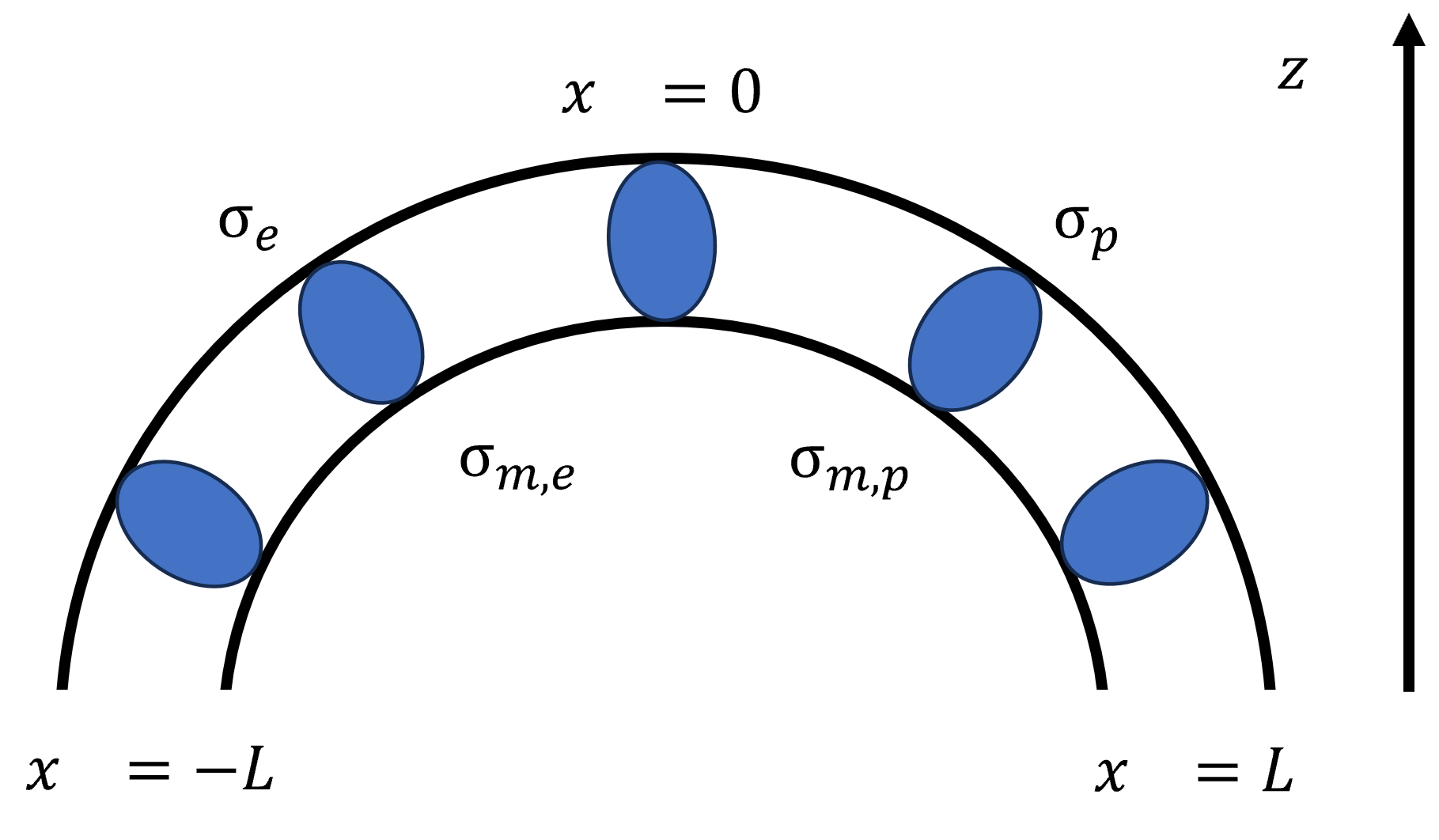
Figure 1: Sketch of the two-component plasma loop model. The vertical axis $z$ is the altitude in the atmosphere; $x$ is the curvilinear abscissa of the loop. $\sigma_{m,\alpha}$,$\sigma_{\alpha}$ with $\alpha=\{e,p\}$ are respectively the surface mass density and the surface charge density of the species $\alpha$.

The first two assumptions imply that the total energy of the system is

$$H=S\biggl{(}\sum_{j=1}^{2N}\sum_{\alpha\in\{e,p\}}\frac{1}{2}\sigma_{m,\alpha}\dot{x}^{2}_{j,\alpha}+E_{el}+U_{g}\biggl{)},$$ (1)

where $\alpha\in\{e,p\}$ denotes the species (here electrons or protons), $g={GM_{\odot}}/{R_{\odot}^{2}}$ is the gravitational field at the surface of the Sun, $x$ is the spatial coordinate (i.e. the curvilinear abscissa of the loop). The total electrostatic energy per section $E_{el}$ reads

$$\begin{gathered}E_{el}=\frac{1}{2}\int_{-L}^{L}dx\rho(x)\phi(x),\end{gathered}$$ (2)

where the charge density

$$\rho(x)=\sum_{j=1}^{2N}\sum_{\alpha\in\{e,p\}}\sigma_{\alpha}\delta(x-x_{j,\alpha}),$$ (3)

is related to the potential $\phi$ by the Poisson equation

$$\frac{\partial^{2}\phi}{\partial x^{2}}=-4\pi\rho.$$ (4)

$U_{g}$ is the total external potential per section and reads

$$U_{g}=\frac{gL\sum_{\alpha\in\{e,p\}}\sigma_{m,\alpha}}{\pi}\sum_{j=1}^{2N}\sum_{\alpha\in\{e,p\}}\cos{\biggl{(}\frac{\pi x_{j,\alpha}}{2L}\biggl{)}}.$$ (5)

In order to use the HMF modelization we first perform the Fourier expansion of the electrostatic energy $E_{el}$. Hereafter we will use the following definition for the Fourier transform

$$f(x)=\sum_{n\in\mathbb{Z}}f_{n}e^{i\frac{\pi nx}{L}},\quad\quad f_{n}=\frac{1}{2L}\int_{-L}^{L}dxf(x)e^{-i\frac{\pi nx}{L}}.$$ (6)

We then introduce the charge imbalances defined as

$$\textbf{q}_{n}=(q_{n,x},q_{n,y})=\sum_{\alpha\in\{e,p\}}\mathrm{sign}{(\sigma_{\alpha})}\textbf{q}_{n,\alpha},$$ (7)

where the vectors $\textbf{q}_{n,\alpha}$ are given by

$$\textbf{q}_{n,\alpha}=\frac{1}{2N}\sum_{j=1}^{2N}\biggl{[}\cos{\biggl{(}\frac{\pi nx_{j,\alpha}}{L}\biggl{)}},\sin{\biggl{(}\frac{\pi nx_{j,\alpha}}{L}\biggl{)}}\biggl{]}.$$ (8)

Performing the Fourier transform (6) of the Poisson equation (4) and applying Eqs. (7-8) we obtain the modes of the potential-density pair as

$$\phi_{n}=\frac{4L^{2}}{\pi n^{2}}\rho_{n},\quad\rho_{n}=-\frac{\sigma_{e}N}{L}(q_{n,x}-iq_{n,y})\quad\forall n\neq 0\quad\rho_{0}=0.$$ (9)

Since each density mode $\rho_{n}$ defined above is related to a specific $\textbf{q}_{n}$, therefore to a vanishing density mode $\rho_{n}$ corresponds a zero charge imbalance. This can be also seen directly from Eq. (7) and Eq. (8). Indeed, if most of the $2N$ particles of a given species are symmetrically concentrated at the bottom of the loop, then $\textbf{q}_{n,\alpha}\approx-1$. Otherwise, if they are uniformly distributed then $\textbf{q}_{n,\alpha}\approx 0$ ($\textbf{q}_{n,\alpha}\approx+1$ corresponds to a situation where most of the particles are concentrated at the top of the loop). As a consequence, if their difference $\textbf{q}_{n}$ does not vanish there is a charge imbalance in the system.
From now on we will refer to the quantities $\textbf{q}_{n,\alpha}$ as the stratification parameters. Performing the Fourier expansion (6) of the charge density (3) and of the electrostatic potential $\phi(x)$ and by using Eqs. (7-9), after some algebra we get the decomposition in Fourier modes of the electrostatic energy per section (2) as

$$E_{el}=\frac{8L(N\sigma_{e})^{2}}{\pi}\sum_{n=1}^{+\infty}\frac{||\textbf{q}_{n}||^{2}}{n^{2}}.$$ (10)

The proportionality to $(N\sigma_{e})^{2}$ arises from the all to all nature of the electrostatic interactions. Its proportionality to $L$ means the larger the size of the system is, the greater is $E_{el}$. The electrostatic energy $E_{el}$ depends on all the charge imbalances $||\textbf{q}_{n}||^{2}$ scaled by $n^{2}$, that is, large-scale modes give larger contribution to the electrostatic energy compared to the small-scale ones. Using Eq. (10) combined with the total energy (1) we derive the equations of motion in the form

$$m_{\alpha}\ddot{x}_{j,\alpha}=eE(x_{j,\alpha})+g\frac{\sum_{\alpha\in\{e,p\}}m_{\alpha}}{2}\sin{\biggl{(}\frac{\pi x_{j,\alpha}}{2L}\biggl{)}},$$ (11)

where the electric field $E$ decomposed in Fourier modes is

$$E(x)=8~{}\mathrm{sign}{(e_{\alpha})}e_{\alpha}n_{S}N\sum_{n=1}^{+\infty}\biggl{[}\frac{q_{n,x}}{n}\sin{\biggl{(}\frac{\pi nx}{L}\biggl{)}}-\frac{q_{n,y}}{n}\cos{\biggl{(}\frac{\pi nx}{L}\biggl{)}}\biggl{]}.$$ (12)

We now implement the HMF assumption by truncating the Fourier expansion at the first mode. The equations above become

$$m_{\alpha}\ddot{x}_{j,\alpha}=e_{\alpha}E(x_{j,\alpha})+g\frac{\sum_{\alpha\in\{e,p\}}m_{\alpha}}{2}\sin{\biggl{(}\frac{\pi x_{j,\alpha}}{2L}\biggl{)}},$$ (13)

and the electric field becomes

$$E(x)=8~{}\mathrm{sign}(e_{\alpha})e_{\alpha}n_{S}N\biggl{[}q_{x}\sin{\biggl{(}\frac{\pi x}{L}\biggl{)}}-q_{y}\cos{\biggl{(}\frac{\pi x}{L}\biggl{)}}\biggl{]}.$$ (14)

In the equations above $\textbf{q}_{\alpha}=\textbf{q}_{1,\alpha}$ are the first mode (large scales) stratification parameters and $q_{x}=q_{1,x}$, $q_{y}=q_{1,y}$ are the first mode charge imbalance components. From now on, unless explicitly stated, we will refer to $\textbf{q}_{\alpha}$ and q respectively as the stratification parameters and the charge imbalance. As one can see, the HMF assumption reduces the computational cost of the electrostatic interactions from $N^{2}$ to $N$.
Let us now comment further on the physics behind the expression of the self-electrostatic interactions. To do so, we use again the electrostatic energy in terms of its Fourier modes (10) truncating the expression at the first mode. After some elementary algebra we get

$$\begin{gathered}E_{el}=E_{0}\sum_{j,k=1}^{2N}\sum_{\alpha,\beta\in\{e,p\}}\tilde{E}_{\alpha,\beta}\textbf{q}_{j,\alpha}\cdot\textbf{q}_{k,\beta},\end{gathered}$$ (15)

where

$$\textbf{q}_{j,\alpha}=\biggl{[}\cos{\biggl{(}\frac{\pi x_{j,\alpha}}{L}\biggl{)}},\sin{\biggl{(}\frac{\pi x_{j,\alpha}}{L}\biggl{)}}\biggl{]},$$ (16)

$\tilde{E}_{\alpha,\beta}=\mathrm{sign}(e_{\alpha})\,\mathrm{sign}(e_{\beta})$, and $\quad E_{0}={4\pi^{-1}Le^{2}n_{S}^{2}N}$. From these expressions it is apparent that the interactions among particles of the same species are described by an antiferromagnetic HMF term while the interactions among particles of different species are, conversely, described by a ferromagnetic HMF term. The antiferromagnetic HMF tends to increase the angle between $\textbf{q}_{j,\alpha}$ and $\textbf{q}_{k,\beta}$ in order to minimise the energy. In terms of physical quantities in the loop this interaction tends to increase the physical distance $x_{j,\alpha}-x_{k,\alpha}$ between two particles of the same species $\alpha$ up to the value $L$ and so such term mimics the electrostatic repulsion between charges of the same sign. The ferromagnetic HMF tends to minimise the energy by decreasing the distance $x_{j,\alpha}-x_{k,\beta}$ between two particles of different species $\alpha,\beta$ up to zero and this mimics the electrostatic attraction between charges of the different sign.

In the following, we consider this plasma model in thermal contact with a thermostat at temperature $T_{0}$ at its boundary (the base of the plasma atmosphere).

2.1 Normalization and central symmetry assumption

To study the dynamics defined by Equations (13), we define the following units for velocity, mass and length

$$\begin{gathered}v_{0}=\sqrt{\frac{k_{B}T_{0}}{m_{e}}},\quad m_{0}=m_{e},\quad L_{0}=\frac{L}{\pi}.\end{gathered}$$ (17)

The choice of units given above implies that the unit of energy is $E_{0}=k_{B}T_{0}$, where $T_{0}$ is the unit of temperature and $k_{B}$ is the Boltzmann constant. For the specific case of the Sun the unit of temperature $T_{0}$ is set equal to the reference temperature of the thermostat (chromosphere), that is $T_{0}=10^{4}$ K. The equations of motion are expressed in dimensionless form as

$$M_{\alpha}\ddot{\theta}_{j,\alpha}=\mathrm{sign}{(e_{\alpha})}CE(\theta_{j,\alpha})+\tilde{F}(\theta_{j,\alpha}),$$ (18)

where the expressions for the external forces and the electrostatic field are

$$\tilde{F}(\theta_{j,\alpha})=\tilde{g}\sin{\biggl{(}\frac{\theta_{j,\alpha}}{2}\biggl{)}},\quad E(\theta)=q_{x}\sin{\theta}-q_{y}\cos{\theta},\\$$ (19)

and the charge imbalance and stratification parameters are given by

$$\textbf{q}=(q_{x},q_{y})=\sum_{\alpha\in\{p,e\}}\mathrm{sign}{(e_{\alpha})}\textbf{q}_{\alpha},\quad\textbf{q}_{\alpha}=\frac{1}{2N}\sum_{j=1}^{2N}(\cos{(\theta_{j,\alpha})},\sin{(\theta_{j,\alpha})}).$$ (20)

In the equations above $M_{\alpha}$ equals $M_{p}={m_{p}}/{m_{e}}$ for the protons; and $M_{e}=1$ for the electrons, while $\theta$ is the dimensionless spatial coordinate. The dynamics is therefore fully identified by the three parameters

$$M=\frac{m_{p}}{m_{e}},\quad C=\frac{8e^{2}L^{2}n_{0}}{\pi k_{B}T_{0}},\quad\tilde{g}=\frac{gL(m_{p}+m_{e})}{2\pi k_{B}T_{0}},$$ (21)

where $n_{0}=Nn_{S}/L$ is the average density of a given species. The quantities $C$ and $\tilde{g}$ measure the strength of the electrostatic interaction and of the external field in units of thermal energy, respectively. Hereafter, unless explicitly stated, we will use dimensionless quantities in all the equations and for all the quantities to be plotted in the figures.
Assuming that all quantities are symmetric respect to the top of the Loop, in terms of the particles phase-space coordinates, corresponds to imposing the following symmetry rules

$$\theta_{j+N,\alpha}=-\theta_{j,\alpha},\quad\dot{\theta}_{j+N,\alpha}=-\dot{\theta}_{j,\alpha};\quad\forall j=1\dots N,$$ (22)

where the first $j=1\dots N$ particles populate one half of the loop $\theta_{j,\alpha}\in[-\pi,0]$ and the remaining particles populate the other half. With such an assumption the system of equations (18) can be reduced to a system of equations for only the first half of the loop as

$$M_{\alpha}\ddot{\theta}_{j,\alpha}=\mathrm{sign}{(e_{\alpha})}CE(\theta_{j,\alpha})+\tilde{F}(\theta_{j,\alpha}),$$ (23)

where the Eqs. (19) become

$$\tilde{F}(\theta_{j,\alpha})=\tilde{g}\sin{\biggl{(}\frac{\theta_{j,\alpha}}{2}\biggl{)}},\quad E(\theta)=q\sin{\theta},$$ (24)

and the Eqs. (20) become

$$q=\sum_{\alpha\in\{p,e\}}\mathrm{sign}{(e_{\alpha})}q_{\alpha},\quad q_{\alpha}=\frac{1}{N}\sum_{j=1}^{N}\cos{(\theta_{j,\alpha})}.$$ (25)

The positions and velocities of particles in the other half of the loop are then determined using Eq. (22).

2.2 Vlasov dynamics and thermal equilibrium solution

In the continuum limit, in terms of phase-space distribution functions the mean-field dynamics of the normalized plasma model given by Eqs. (23) is governed by a system of two Vlasov equations

$$\frac{\partial f_{\alpha}}{\partial t}+\frac{p}{M_{\alpha}}\frac{\partial f_{\alpha}}{\partial\theta}+F_{\alpha}[f_{\alpha}]\frac{\partial f_{\alpha}}{\partial p}=0,\quad F_{\alpha}=-\frac{\partial H_{\alpha}}{\partial\theta},$$ (26)

where $f_{\alpha}$ are the single-particle distribution functions for both species, and $H_{\alpha}$ are the mean-field Hamiltonians

$$H_{\alpha}=\frac{p^{2}}{2M_{\alpha}}+\mathrm{sign}{(e_{\alpha})}C\phi(\theta)+2\tilde{g}\cos{\biggl{(}\frac{\theta}{2}\biggl{)}};\quad\phi(\theta)=q\cos{\theta},$$ (27)

where

$$q=\sum_{\alpha\in\{e,p\}}\mathrm{sign}{(e_{\alpha})}q_{\alpha},\quad q_{\alpha}=\int_{-\pi}^{\pi}d\theta\int_{-\infty}^{\infty}dp\cos{\theta}f_{\alpha}(\theta,p).$$ (28)

In virtue of the Jeans’ theorem (see e.g. Nicholson (1983)), all stationary solution of the system (26) are functions the sole mean-field Hamiltonians (27). Technically speaking, in general, the stationary solution of a Vlasov equation is function of all the constants of motion. Here, since our model is one-dimensional the only independent constants of motion are the mean-field Hamiltonians $H_{\alpha}$. Among all the solutions of the system above, the thermal equilibrium one has the following expression

$$\begin{gathered}f_{\alpha}(\theta,p)=\frac{e^{-\frac{H_{\alpha}}{T}}}{Z_{\alpha}},\quad Z_{\alpha}=\int_{-\pi}^{\pi}d\theta\int_{-\infty}^{+\infty}dp\,e^{-\frac{H_{\alpha}}{T}},\end{gathered}$$ (29)

where $f_{\alpha}$ is normalized to 1 for both species. To evaluate the explicit functional form of $f_{\alpha}$, one needs the exact value of $q$. As a consequence, we transform (29) into an algebraic scalar equation in $q$ of the form

$$\begin{gathered}q=\sum_{\alpha\in\{e,p\}}\mathrm{sign}{(e_{\alpha})}\int_{-\infty}^{+\infty}dp\int_{-\pi}^{\pi}d\theta\cos{\theta}\frac{e^{-\frac{H_{\alpha}[q]}{T}}}{\int_{-\infty}^{+\infty}dp\int_{-\pi}^{\pi}d\theta e^{-\frac{H_{\alpha}[q]}{T}}},\end{gathered}$$ (30)

whose solution is $q=0$ (and so $\phi=0$). Therefore, the equilibrium solution of a two-component plasma model, where the two species are subject to the same external potential, requires a vanishing self-electrostatic potential, (i.e., $\phi=0$). The thermal solution for the plasma atmosphere model is the so-called isothermal atmosphere given by

$$f_{\alpha}(\theta,p)=\frac{e^{-\frac{\tilde{H}_{\alpha}}{T}}}{Z_{\alpha}},\quad Z_{\alpha}=\int_{-\pi}^{\pi}d\theta\int_{-\infty}^{+\infty}dp\,e^{-\frac{\tilde{H}_{\alpha}}{T}}\,$$ (31)

where $\tilde{H}_{\alpha}$ are the mean-field Hamiltonians (27) with $\phi=0$, that is

$$\tilde{H}_{\alpha}=\frac{p^{2}}{2M_{\alpha}}+2\tilde{g}\cos{\biggl{(}\frac{\theta}{2}\biggl{)}}.$$ (32)

The knowledge of the distribution functions allows us to compute the number densities $n_{\alpha}$ and the temperatures profiles $T_{\alpha}$ using the standard kinetic definitions (see e.g. Nicholson (1983)). For the number densities we get

$$n_{\alpha}(\theta)=\frac{e^{-\frac{2\tilde{g}}{T}\cos{\bigl{(}\frac{\theta}{2}}\bigl{)}}}{\int_{-\pi}^{\pi}d\theta e^{-\frac{2\tilde{g}}{T}\cos{\bigl{(}\frac{\theta}{2}}\bigl{)}}},$$ (33)

and for the kinetic temperatures

$$T_{\alpha}(\theta)=T.$$ (34)

2.3 The thermostat temperature fluctuations

Starting from a thermal equilibrium state (31) with temperature $T_{0}=1$, the out of equilibrium state is induced by introducing fluctuations in the value of the temperature of the thermostat. In practice, we first increase the temperature from the initial equilibrium value $T_{0}$ up to $T>T_{0}$ for a finite time interval $\tau$, of length smaller than the relaxation time $t_{R}$ to equilibrium at temperature $T$. After a time $\tau$ the temperature of the thermostat is reverted to $T_{0}$ for a finite time interval $t_{w}$ again much smaller than the relaxation time $t_{R}^{\prime}$ back to $T_{0}$. Iterating this procedure prevents the system to relax to a thermal equilibrium at either $T_{0}$ or $T$. The values of $t_{w}$ and $T$ have been sorted from different probability distributions $\eta(t_{w})$ and $\gamma(T)$.

3 Temporal coarse-graining

Under the conditions prescribed above we now define the coarse-graining time scale $\tilde{t}$ such that

$$\tau,\langle t_{w}\rangle\ll\tilde{t}\ll\tilde{t}_{R},$$ (35)

where $\tilde{t}_{R}\equiv{\rm min}(t_{R};t_{R}^{\prime})$. The temporal coarse-grained phase-space distribution function, defined as the time average of $f_{\alpha}$ over $\tilde{t}$, reads as

$$\begin{gathered}\tilde{f}_{\alpha}(\theta,p,\tilde{t})=\langle f_{\alpha}\rangle_{\tilde{t}}=\frac{1}{\tilde{t}}\int_{\tilde{t}}dtf_{\alpha}(\theta,p,t),\end{gathered}$$ (36)

and the time-averaged Vlasov dynamics over $\tilde{t}$ becomes

$$\frac{f_{\alpha}(\theta,p,\tilde{t})-f_{\alpha}(\theta,p,0)}{\tilde{t}}+\frac{p}{M_{\alpha}}\frac{\partial\tilde{f}_{\alpha}}{\partial\theta}+\biggl{\langle}\tilde{F}_{\alpha}\frac{\partial f_{\alpha}}{\partial p}\biggl{\rangle}_{\tilde{t}}=0.$$ (37)

Given the condition $\tilde{t}\ll\tilde{t}_{R}$, during the time interval $\tilde{t}$ the system energy can not be redistributed along the loop. We can therefore approximate $f_{\alpha}$ with its time average $f_{\alpha}=\tilde{f}_{\alpha}$, while the finite difference in the left hand side of (37) becomes a time derivative. We then get

$$\begin{gathered}\frac{\partial\tilde{f}_{\alpha}}{\partial\tilde{t}}+\frac{p}{M_{\alpha}}\frac{\partial\tilde{f}_{\alpha}}{\partial\theta}+\tilde{F}_{\alpha}[\tilde{f}_{\alpha}]\frac{\partial\tilde{f}_{\alpha}}{\partial p}=0.\end{gathered}$$ (38)

The thermostat at the bottom boundary of the system induces an incoming flux defined at a given time by

$$J_{T,\alpha}=\int_{0}^{+\infty}dp\frac{p}{TM_{\alpha}}e^{-\frac{p^{2}}{2TM_{\alpha}}},$$ (39)

where the value of $T$ is drawn from the distribution $\gamma(T)$ during the time intervals of length $\tau$; while $T=1$ during time intervals of length $t_{w}$ drawn from $\eta(t_{w})$.
We now compute the temporal coarse-grained flux by taking the time-average of (39), obtaining

$$J_{\alpha}=\frac{t_{t_{w}}}{\tilde{t}}\langle J_{T,\alpha}\rangle_{t_{t_{w}}}+\frac{t_{\tau}}{\tilde{t}}\langle J_{1,\alpha}\rangle_{t_{\tau}},$$ (40)

where $\tilde{t}=t_{t_{w}}+t_{\tau}\quad t_{t_{w}}=\sum_{i=1}^{n_{p}}t_{w_{i}}\quad t_{\tau}=n_{p}\tau$ and $n_{p}$ is the total number of temperature increments within $\tilde{t}$. Assuming $\tau,t_{w_{i}}\ll\tilde{t}$ implies that the amount of temperature fluctuations in such interval is large enough to justify the use of an ergodic assumption. We can therefore replace the time average over $t_{t_{w}}$ with the average with respect to its probability distribution, as

$$\langle J_{T,\alpha}\rangle_{t_{t_{w}}}\\ =\int_{1}^{+\infty}dT\gamma(T)J_{T,\alpha}.$$ (41)

Furthermore, the assumption $\tau,t_{w}\ll\tilde{t}$ also implies $t_{t_{w}}=\sum_{i=1}^{n_{p}}t_{w_{i}}=n_{p}\langle t_{w}\rangle_{\eta}$ so that the coarse-grained flux becomes

$$J_{\alpha}=\int_{0}^{+\infty}dpp\tilde{f}_{\alpha}(p),$$ (42)

where $\tilde{f}_{\alpha}(p)$ is defined by

$$\tilde{f}_{\alpha}(p)=\frac{A}{M_{\alpha}}\int_{1}^{+\infty}dT\frac{\gamma(T)}{T}e^{-\frac{p^{2}}{2TM_{\alpha}}}+\frac{1-A}{M_{\alpha}}e^{-\frac{p^{2}}{2M_{\alpha}}},$$ (43)

and $A$ is

$$A=\frac{\tau}{\tau+\langle t_{w}\rangle_{\eta}}.$$ (44)

In practice, the dynamics of a two component plasma coupled to a time fluctuating thermostat at a given boundary is described, at the temporal coarse-grained level, by a set of Vlasov equations (38) for the two species coupled to two incoming effective fluxes (42) at the boundary. The latter are generated by the non-thermal distributions $\tilde{f}_{\alpha}$ given in Eq. (43).
In the formalism introduced above, it is possible to evaluate an analytic expression for the coarse-grained phase-space distribution functions in the stationary configuration. To do so, one has first to determine such phase-space distributions at the boundary in the stationary configuration. This can be carried out imposing the stationarity and the continuity condition at the boundary, together with the symmetry condition in the momentum space

$$\frac{\partial\tilde{f}_{\alpha}}{\partial\tilde{t}}=0,\quad\mathcal{N}_{\alpha}\tilde{f}_{\alpha}(p)=\tilde{f}_{\alpha}(-\pi,p),\quad\tilde{f}_{\alpha}(-\pi,p)=\tilde{f}_{\alpha}(-\pi,-p),\quad p>0.$$ (45)

In the expressions above $\mathcal{N}_{\alpha}$ are normalization constants. We can now build up the solution in the whole phase space using the Jeans theorem. We then get

$$\tilde{f}_{\alpha}(\theta,p)=\mathcal{N}_{\alpha}\biggl{(}A\int_{1}^{+\infty}dT\frac{\gamma(T)}{T}e^{-\frac{H_{\alpha}}{T}}+(1-A)e^{-H_{\alpha}}\biggl{)},$$ (46)

where $H_{\alpha}$ are the mean-field Hamiltonians defined in Eq. (27). The constants $\mathcal{N}_{\alpha}$ are fixed by the normalization condition for the two species

$$\int_{-\pi}^{\pi}d\theta\int_{-\infty}^{+\infty}dp\tilde{f}_{\alpha}(\theta,p)=1.$$ (47)

Since $H_{\alpha}$ depends on $\tilde{f}_{\alpha}(\theta,p)$ only through the electrostatic potential $\phi$, this is a self-consistent problem that can be solved with respect to $\phi$ as done for the equilibrium solution (30) obtaining $\phi=0$. As a consequence, the mean-field-Hamiltonians $H_{\alpha}$ reduce to $\tilde{H}_{\alpha}$ as in Eq. (32). The first term in the r.h.s. of Eq. (46) is induced by the temperature fluctuations of the thermostat and is a superposition of Boltzmann exponential distributions, each of which has a temperature $T>1$ weighted with the probability $\gamma(T)$. Such term introduces the suprathermal contribution and from now on will be referred to as the multitemperature population.
The second term in the r.h.s. of (46) is proportional to a Boltzmann exponential at $T=1$, due to the fact that along each interval of length $t_{w}$ the thermostat is brought back to the temperature $T=1$. From now on we will refer to this term as the thermal population. The relative contribution of the multitemperature and thermal populations is weighted by the factor $A$ given by Eq. (44), corresponding to the fraction of time in which the thermostat is set at one of the temperatures of the multitemperature population.
The shape of the distribution functions depends only on the mean-field Hamiltonians $\tilde{H}_{\alpha}$, since the system is ruled by a Vlasov-type dynamics.
Our formalism allows one to discuss the physics in the stationary configuration in terms of velocity filtration. Given the presence of suprathermal tails in the distribution functions (as induced by the multitemperature population) and an external field, the temperature inversion process is expected to take place. This can be easily verified by computing the number densities $n_{\alpha}$ and the kinetic temperatures $T_{\alpha}$ from the equations (46), using the standard kinetic definitions (see e.g. Nicholson 1983). For the number densities we get

$$\tilde{n}_{\alpha}(\theta)=\frac{A\int_{1}^{+\infty}dT\frac{\gamma(T)}{\sqrt{T}}e^{-\frac{2\tilde{g}}{T}\cos{(\frac{\theta}{2})}}+(1-A)e^{-2\tilde{g}\cos{(\frac{\theta}{2})}}}{A\int_{1}^{+\infty}dT\frac{\gamma(T)}{\sqrt{T}}\int_{-\pi}^{\pi}d\theta e^{-\frac{2\tilde{g}}{T}\cos{(\frac{\theta}{2})}}+(1-A)\int_{-\pi}^{\pi}d\theta e^{-2\tilde{g}\cos{(\frac{\theta}{2})}}},$$ (48)

while for the kinetic temperatures

$$\tilde{T}_{\alpha}(\theta)=\frac{A\int_{1}^{+\infty}dT\gamma(T)\sqrt{T}e^{-\frac{2\tilde{g}}{T}\cos{(\frac{\theta}{2})}}+(1-A)e^{-2\tilde{g}\cos{(\frac{\theta}{2})}}}{A\int_{1}^{+\infty}dT\frac{\gamma(T)}{\sqrt{T}}e^{-\frac{2\tilde{g}}{T}\cos{(\frac{\theta}{2})}}+(1-A)e^{-2\tilde{g}\cos{(\frac{\theta}{2})}}}.$$ (49)

In the next Section the above formulas will be evaluated for different choices of model parameters and compared with the output of kinetic numerical simulations.

4 Comparison with numerical simulations

We validated our model with $N-$particle numerical simulations where we integrated the equations of motion (23) of the system. In the numerical experiments discussed here, as a rule, we fixed $N=2^{21}$ and used a fourth-order symplectic algorithm (see e.g. Candy & Rozmus 1991) with fixed time step $\delta t=10^{-4}$. We modelled the incoming energy flux from the fluctuating thermostat with the standard technique (see Tehver et al. 1998; Landi & Pantellini 2001) such that, when a particle of a given species crosses the boundary, it is re-injected in the system (at the bottom) with a positive velocity sampled from the flux density argument of Eq.(39). We note that, naively re-introducing the particle with a new velocity extracted from a (half) Gaussian at temperature $T$, would break the stationary thermal equilibrium solution, as re-injected particles would have, by construction, a higher chance of having a near zero velocities (see e.g. Lepri et al. (2021) and references therein).

4.1 Stationary state and model parameters

Motivated by the modelization of the Sun atmosphere, we set the distributions of the temperature fluctuations $\gamma(T)$ and waiting times $\eta(t_{w})$ as

$$\gamma(T)=\frac{1}{T_{p}}e^{-\frac{(T-1)}{T_{p}}},\quad T>1,\quad\eta(t_{w})=\frac{1}{\langle t_{w}\rangle_{\eta}}e^{-\frac{t_{w}}{\langle t_{w}\rangle_{\eta}}}.$$ (50)

The idea is that the chromospheric (i.e. the thermostat) temperature fluctuates randomly in time, and the strong temperature increments (i.e., those producing a large $T$), are rather rare (see Barbieri et al. 2024). This established, we tune the remaining parameters ($A,\tilde{g},C,T_{p}$) accordingly. In Figs. 2-6 (left panels) we show the time evolution of the kinetic energies $K_{\alpha}$ (top panels) and of the stratification parameters $q_{\alpha}$ (bottom panels) evaluated in the numerical simulations for different choices of the parameter set as

$$K_{\alpha}=\frac{1}{N}\sum_{i=1}^{N}\frac{p_{j,\alpha}^{2}}{2M_{\alpha}},\quad q_{\alpha}=\frac{1}{N}\sum_{j=1}^{N}\cos{(\theta_{j,\alpha})},$$ (51)

together with their theoretical value (indicated by the straight solid lines) in the stationary configuration, given by

$$q_{\alpha,SS}=\int_{-\pi}^{\pi}d\theta\int_{-\infty}^{+\infty}dp\cos{\theta}\tilde{f}_{\alpha}(\theta,p),\quad K_{\alpha,SS}=\int_{-\pi}^{\pi}d\theta\int_{-\infty}^{+\infty}dp\frac{p^{2}}{2M_{\alpha}}\tilde{f}_{\alpha}(\theta,p).$$ (52)

In all cases, both $K_{\alpha}$ and $q_{\alpha}$ relax towards their predicted stationary value. In the right panels of the same figures we show the kinetic temperature $T_{e}$ together with the number density $n_{e}$ for the electrons—the profiles for the protons having the same shape—as a function of the spatial coordinate $\theta$. The latter were computed numerically using the standard kinetic definitions (see e.g. Nicholson 1983) for a single snapshot in the stationary state and then time averaging over subsequent snapshots. In addition, using Eqs. (48-49) we have also computed their theoretical expressions. In all cases presented here, we observe a very good match between the numerical and analytical curves.

4.1.1 The fraction of time $A$

As apparent from Eq. (44), the parameter $A$ controls the fraction of time in which the thermostat is at a given value $T$ sorted from $\gamma(T)$. In Figure 2 we present two cases: $A=0.5(\tau=0.01,\langle t_{w}\rangle_{\eta}=0.01)$ and $A=0.25(\tau=0.01,\langle t_{w}\rangle_{\eta}=0.03)$. All the other parameters are fixed to $\tilde{g}=1,T_{p}=4,C=400,M=100$.
Increasing $A$ corresponds to an increment of the weight of the multitemperature population in Eq. (46) and therefore more energy is injected into the plasma. As a consequence, the plasma becomes less stratified in density (see variation of $\tilde{n}_{\alpha}$ and of the stratification parameters $q_{\alpha}$ in Figure 2). For the same reason, the mean value of the kinetic energies $K_{\alpha}$ in the non-equilibrium stationary configuration increases, as the profile of the kinetic temperatures $\tilde{T}_{\alpha}$ does at each in point of the space.

Figure 2: Left panels: Evolution of protons (red for $A=0.25$ and green for $A=0.5$) and electrons (blue for $A=0.25$ and orange for $A=0.5$) kinetic energies $K_{\alpha}$ (top panel) and stratification parameters $q_{\alpha}$ (bottom panel) as numerically computed from simulations via Eq.(51), together with theoretical prediction for their mean value (black horizontal lines, see Eq. (52)). Right panel: numerical density (in blue for $A=0.25$ and in red for $A=0.5$) and temperature (same rule of colours) of electrons vs curvilinear abscissa of the loop $\theta$. Gray curves denote the corresponding theoretical predictions from analytical formulas Eqs (48)-(49).

4.1.2 The intensity of temperature increments $T_{p}$

The parameter $T_{p}$ (see Eq. 50) controls the mean value of the (exponential) distribution of the temperature fluctuations. In Figure 3 we present two cases: $T_{p}=1$ and $T_{p}=4$. As above, all the other parameters are fixed and are $A=0.5(\tau=0.01,\langle t_{w}\rangle_{\eta}=0.01),\tilde{g}=1,C=400,M=100$. Also in this case, increasing the value of $T_{p}$ makes the energy injected by the multitemperature population to increase. We thus obtain the same behaviour as in the previous case (Figure 2) for all quantities.

Figure 3: Left panels: Evolution of protons (red for $T_{p}=4$ and green for $T_{p}=1$) and electrons (blue for $T_{p}=4$ and orange for $T_{p}=1$) kinetic energies $K_{\alpha}$ (top panel) and stratification parameters $q_{\alpha}$ (bottom panel) as numerically computed from simulations via Eq. (51), together with theoretical prediction for their mean value (black horizontal lines, see Eq. (52)). Right panel: numerical density (in blue for $T_{p}=4$ and in red for $T_{p}=1$) and temperature (same rule of colours) of electrons vs curvilinear abscissa of the loop $\theta$. Gray curves denote the corresponding theoretical predictions from analytical formulas Eqs (48)-(49).

4.1.3 The strength of the electrostatic interactions $C$

The parameter $C$ controls the strength of the electrostatic interactions between particles. In Figure 4 we report the two cases $C=100$ and $C=400$. All the other parameters are fixed such that $A=0.5(\tau=0.01,\langle t_{w}\rangle_{\eta}=0.01),T_{p}=4,\tilde{g}=1,M=100$. This Figure clearly shows that the electrostatic interaction $C$ does not play any significant role in shaping the inverted density-temperature profiles, as obvious from the theory since $\phi=0$, cfr. Sect. 3.

Figure 4: Left panels: Evolution of protons (red for $C=400$ and green for $C=100$) and electrons (blue for $C=400$ and orange for $C=100$) kinetic energies $K_{\alpha}$ (top panel) and stratification parameters $q_{\alpha}$ (bottom panel) as numerically computed from simulations via Eq. (51), together with theoretical prediction for their mean value (black horizontal lines, see Eq. (52)). Right panel: numerical density (in yellow for $C=400$ and in black for $C=100$) and temperature (same rule of colours) of electrons vs curvilinear abscissa of the loop $\theta$. Red curves denote the corresponding theoretical predictions from analytical formulas Eqs (48)-(49).

4.1.4 The stratification parameter $\tilde{g}$

This parameter determines the strength of the external stratification field in units of the thermal energy $k_{B}T_{0}$ of the thermostat (i.e., the chromosphere). In Figure 5 we present two cases: $\tilde{g}=0.5$ and $\tilde{g}=1$. All the other parameters are as before. The expressions of the distribution functions of the theory reported in Eq. (46) depend only on $\tilde{H}_{\alpha}$. At the bottom (i.e., $\theta=-\pi$), the mean-field Hamiltonians $\tilde{H}_{\alpha}$ are the same for both species and read

$$\tilde{H}_{\alpha}(p,\theta=-\pi)=\frac{p^{2}}{2M_{\alpha}}.$$ (53)

Therefore, the two distribution functions have a fixed width in momentum space that is independent of the specific value of $\tilde{g}$. Hence, also the kinetic temperature at $\theta=-\pi$ is independent of $\tilde{g}$, as apparent in Figure 5.
In the right plot of Figure 5 we show that, by increasing the value of $\tilde{g}$, the kinetic temperature grows with a stronger gradient going from the bottom ($\theta=-\pi$) to the top ($\theta=0$). In practice, as implied by Eq. (46), with higher values of $\tilde{g}$, only the Boltzmann factors with large values of the temperature in the multitemperature population can give a contribution at higher altitudes. In practice, from all the possible value extracted from $\gamma(T)$, only high $T$ temperature fluctuations give a sufficient amount of kinetic energy to the particles so that they can climb the gravitational well up to the top of the system $\theta=0$. We note that, this is essentially Scudder’s gravitational filtering mechanism.

Figure 5: Left panels: Evolution of protons (red for $\tilde{g}=1$ and green for $\tilde{g}=0.5$) and electrons (blue for $\tilde{g}=1$ and orange for $\tilde{g}=0.5$) kinetic energies $K_{\alpha}$ (top panel) and stratification parameters $q_{\alpha}$ (bottom panel) as numerically computed from simulations via Eq. (51), together with theoretical prediction for their mean value (black horizontal lines, see Eq. (52)). Right panel: numerical density (in blue for $\tilde{g}=1$ and in red for $\tilde{g}=0.5$) and temperature (same rule of colours) of electrons vs curvilinear abscissa of the loop $\theta$. Gray curves denote the corresponding theoretical predictions from analytical formulas Eqs (48)-(49).

4.1.5 Varying the temperature fluctuations distribution $\gamma(T)$

Finally, we change the distribution of temperature increments $\gamma(T)$. We consider here the case of a one sided Gaussian $\gamma(T)$ distribution

$$\gamma(T)=\frac{2}{\sqrt{2\pi T_{p}^{2}}}e^{-\frac{(T-1)^{2}}{2T_{p}^{2}}},\quad T>1.$$ (54)

In Figure 6 we show the case for the following values of the system’s parameters: $A=0.5(\tau=0.01,\langle t_{w}\rangle_{\eta}=0.01),\tilde{g}=1,T_{p}=4,C=400,M=100$. As expected, temperature increments still give origin to temperature inversion independently of the specific shape of $\gamma(T)$.

Figure 6: Left panels: Evolution of protons (green) and electrons (red) kinetic energies $K_{\alpha}$ (top panel) and stratification parameters $q_{\alpha}$ (bottom panel) as numerically computed from simulations via (51), together with theoretical prediction for their mean value (black horizontal lines, see Eq. (52)). Right panel: numerical density and temperature (red) of electrons vs curvilinear abscissa of the loop $\theta$. Gray curves denote the corresponding theoretical predictions from analytical formulas Eqs (48)-(49).

4.2 Limits of the theoretical approach

We now discuss the limits of the theoretical approach, using numerical simulations. For the sake of simplicity, we focus on the case in which the temperature oscillates between the the two values $T=1$ and $T=T_{p}$ with a fixed waiting time $t_{w}$. In this setup the distributions $\gamma(T)$ and $\eta(t_{w})$ are given by

$$\gamma(T)=\delta(T-T_{p}),\qquad\eta(t_{w})=\delta(t-t_{w}).$$ (55)

In Figure 7, we report the results obtained by varying $\tau$, with $\tau=t_{w}$. The other parameters are fixed to $C=400,T_{p}=4,\tilde{g}=1,M=100$.
We observe how increasing both $\tau$ and $t_{w}$ and retaining the ratio $A=\frac{\tau}{\tau+t_{w}}$ fixed to $0.5$, the theoretical equations computed using Eq. (46) start failing in reproducing the density-temperature profiles evaluated from the numerical simulations. In particular, in the left panels the time scales $\tau$ and $t_{w}$ are so small that the particles do not have enough time to relax to a thermal configuration, neither at $T=T_{p}$ or at $T=1$. The system is therefore locked in a non-equilibrium stationary configuration and the inverted density-temperature profiles computed numerically are well reproduced by the theoretical counterparts. Technically speaking, the inverted density-temperature profiles shown in Fig. 7 are obtained by time-averaging over several snapshots from the $t_{1}=300$ to the end time $t_{2}=1000$. Since the system is in a stationary state these profiles are independent on the length and on the location along the stationary state of the interval $t_{2}-t_{1}$.
For the other cases, the density-temperature profiles are numerically evaluated in the same way. As both $\tau$ and $t_{w}$ increase, the kinetic energy starts to develop large amplitude oscillations. This arises from the fact that when moving towards a regime (shown in the two right columns of the Figure 7) in which both $\tau$ and $t_{w}$ are large enough (i.e. comparable to the relaxation time) such that the system evolves in time passing from a thermal configuration at $T=T_{p}$ to a thermal configuration at $T=1$ (see Figure 8).
Of course, in all cases except when $\tau=t_{w}=0.1$, since the system is no longer locked in a stationary configuration, the theory can not be applied and thus the numerically recovered density-temperature profiles evaluated via time averaging do not match the theoretical counterparts. Moreover, since the system is no more locked in a stationary state, the numerical density-temperature profiles depend explicitly on the length and on the location of the time average interval $t_{2}-t_{1}$ for the specific run.

Figure 7: First row: kinetic energies of the electrons for four different couples of values of $\tau=t_{w}={0.1,20,200,600}$ from left to right. Second row: electrons temperature-density profiles numerically evaluated time averaging over the interval $t_{1}=300$ and $t_{2}=1000$ (red for temperature and blue for density) together with the theoretical predictions in grey and calculated via Eqs. (48)-(49).

Figure 8: Left: electrons Kinetic energy as a function of time. Right: electrons densities and temperatures for the two thermal configurations $T=T_{p}=4$ and $T=1$. In blue and magenta respectively the numerical temperature and the numerical density for the case $T=T_{p}=4$, together with their respective theoretical equilibrium counterparts in grey and calculated via Eqs. (33)-(34). In red and black respectively the numerical temperature and the numerical density for the case $T=1$, together with their respective theoretical equilibrium counterparts in grey and calculated via Eqs. (33)-(34).

Figure 9: Kinetic temperature (in K, left panel) computed via (49) and number density computed via (48) (right panel) scaled by the mean number density $n_{0}=2.5\cdot 10^{9}\mathrm{cm}^{-3}$ as a function of the height (in km) for different values of $A$ passing from $A=1$ to $A=0.01$ as listed in the legend.

Figure 10: Left panel: temperature at base $T_{b}$ of the atmosphere $z=0$ computed via Eq. (49) against the parameter $A$ Eq. (44). The red horizontal line is $T_{b,obs}=1.2\times 10^{4}$ K. Right panel: the temperature at the top $T_{t}$ computed via Eq. (49) as function of the mean-value of the temperature fluctuations $T_{p}$ for $A=1$.

Figure 11: Left panel: electron velocity distribution functions (VDFs) computed via (46) normalized by the electron number densities (computed via (48)) at the base of the atmosphere at $z=z_{1}=2.3\times 10^{3}\mathrm{km}$ (the base of the transition region) for different values of $A$. In the central panel a magnification of the central region of the same VDFs are shown to emphasise the central thermal (Gaussian) core. In the right panel are depicted the electron VDFs in the corona $z=z_{3}$ for the same values of $A$ of the other panels. In this panel all the electron VDFs are collapsed onto each other because of velocity filtration.

Figure 12: Left panel: electron DFs (computed via 46 normalized by the electron number densities (computed via 48) for $A=0.02$, computed at three increasing heights ($z=z_{1},z_{2},z_{3}$) listed in the legend as a function of the signed kinetic energy. In the right panel, a magnification of the central region of the same DFs is shown to appreciate the disappearance of the Gaussian profile with height, as expected when velocity filtration is at work.

5 Application to the solar atmosphere

Here we show the application of the temporal coarse-graining to predict the inverted density-temperature profiles of the Sun atmosphere. To compute such profiles we have used Eqs. (48)-(49), and Eqs. (46) for the distribution functions. We put the base of the model at $z_{b}=2\times 10^{3}$ km (i.e., at the base of the transition region in the Sun atmosphere) and the top at $z_{t}=2.2\times 10^{4}$ km (i.e., in the corona). We then fix the length $2L$ of half of the loop via the following equation

$$2L=(z_{t}-z_{b})\pi=2\pi\times 10^{4}{\rm km},\quad z=\frac{2L}{\pi}\cos{\biggl{(}\frac{\pi x}{2L}\biggl{)}},$$ (56)

that corresponds to the typical length of a coronal loop in the solar atmosphere. With such choice, the dimensionless parameter $\tilde{g}$ is fixed to $\tilde{g}=16.64$. For the distribution of the temperature fluctuations and the waiting times, we use Equations (50) discussed in section 4 above. Thus, we are now left with the two free parameters $T_{p}$ and $A$. We initially fix the value of $A$ to $1$ and vary $T_{p}$.
As shown in Section 4, increasing the value of $T_{p}$ results in increasing the values of the temperature profile. In order to have a temperature of the order of $10^{6}$ K at the top of the loop, we must increase $T_{p}$ up to a value around $10^{6}$ K (as shown in the right panel of figure 10). Therefore, from now on, we fix $T_{p}=90$ (that correspond to a temperature of $9\times 10^{5}$ K). From the left panels of figures 10 and 9 we observe that for $A=1$ we have a temperature at the base of the order of $T_{b}=5\times 10^{5}$ K. Such value is far greater than the observed one, the latter being smaller than $T_{b,obs}=1.2\times 10^{4}{\rm K}$, for the chromospheric temperature varies between $8\times 10^{3}$ and $1.2\times 10^{4}$ K, see Molnar et al. (2019).
In the previous section we have shown how the temperature at the base of the loop $T_{b}$ decreases with decreasing $A$ (see figure 2). In Figure 10 we plot $T_{b}$ as a function of $A$. We observe that at around A=$0.022$ the temperature $T_{b}$ crosses the upper limit value $T_{b,obs}$. Combining these two properties that relate $T_{p}$ to $A$, in Figure 9 we show how the inverted density-temperature profiles with $A=0.02$ and $0.01$ (i.e. very rare temperature increments with $T_{p}=90$) are similar to the one observed in the Sun atmosphere. These profiles start from $T_{b}\sim 1.1\times 10^{4}$ K, they have an initial rapid rise in temperature (the transition region) followed by a slower increase in the above region (i.e. the solar corona).
This change of the shape caused by varying the parameter $A$ can be understood in terms of velocity filtration, as it is apparent from the structure of the electron velocity distribution functions (VDFs) at the base of the model ($z=z_{1}=2.3\times 10^{3}$ km) as shown in Figure 11 where we plot in a semilogarithmic scale the distribution of the signed electron kinetic energy $\tilde{f}_{e}(\text{sign}(p)\,p^{2}/2)$ divided by the density. By doing this, it becomes clearer whether the distribution function in question is thermal or not, since for a thermal distribution (i.e. a Gaussian) one would get two straight lines symmetric with respect to zero. As can be seen from the left and the middle panels of Figure 11, the thermal (Gaussian) part of the electron VDFs increasingly dominates the core of the distribution, as the value of $A$ decreases. This is the reason why the temperature at the base decreases crossing $T_{b,obs}=1.2\times 10^{4}$ K and tends to $T_{0}=10^{4}$ K. Moreover, by fixing $A=0.02$, from Figure 12 we observe that, in virtue of the energy conservation (thanks to the velocity filtration mechanism), the cold central thermal core of the electron DFs at the base of the model $z=z_{1}=2.3\times 10^{3}$ km progressively disappears by passing through the transition region $z=z_{2}=2.3\times 10^{3}$ km and is totally filtered out in the corona $z=z_{3}=1.1\times 10^{4}$ km. As a consequence of this, one has a rapid increase of temperature through the transition region and a slow increase of temperature in the corona.
In right panel of Figure 11 we can observe that all the electron DFs rescaled by the density in the corona at $z=z_{3}=1.1\times 10^{4}$ km for all the values of $A$ collapse onto each other, due to the fact that the central thermal core has been filtered out in the corona itself. Since the rescaled distribution functions are the same for all values of $A$, then the temperatures collapse to the same curve in the corona as shown in the left panel of Figure 9.
The number density profiles are inverted respect to the temperature profiles with an initial strong negative gradient (the transition region) followed by a slower decrease within the corona. By decreasing the value of $A$, the number density at the bottom of the system increases and at the same time the number density at the top decreases. Again this is due to the fact that the cold population in Equation (46) becomes more and more pronounced for decreasing values of $A$, that is, we now have more particles that are not able to climb higher in the gravity well. Since the total number of particles is fixed independently on the values of $A$ as dictated by the normalization condition (47) then, if the density at the bottom increases, the density at the top (the corona) should naturally decrease.

6 Summary and perspectives

In this paper we have presented a novel formalism to treat the plasma dynamics in contact with a thermostat whose temperature fluctuates in time, (see also Barbieri et al. 2024) based on temporal coarse-graining. We have shown how the multi-component (in the case discussed here, electrons and protons) plasma dynamics can be efficiently modelled in terms of the temporal-coarse-grained distribution functions $\tilde{f}_{\alpha}$ for the two species. The dynamics of the latter is governed by the effective system of Vlasov equations (38) in contact with the non-thermal distributions $\tilde{f}_{\alpha}(p)$ at its boundary (43).
We have obtained analytical expressions for the distribution functions of the two species in the non-equilibrium stationary configuration (46), in terms of the mean field Hamiltonians $\tilde{H}_{\alpha}$ Eq.(32). In this setup we can interpret the anti-correlated density-temperature profiles in terms of velocity filtration, in analogy to the Scudder mechanism; the suprathermal tails are not imposed as in the Scudder approach but are naturally induced by the temperature fluctuations of the thermostat.
We have tested the theoretical predictions for temperature inversion against numerical simulations, finding an excellent agreement between the theory and the numerical results. In addition, we have applied our theoretical formalism to the specific case of the Sun atmosphere, showing the important played by the parameter $A$ in shaping the inverted density-temperature profile. Moreover, in the condition of very rare temperature fluctuations $A\sim 0.02$ at $T_{p}\sim 10^{6}$ K we were able to produce an inverted temperature-density profile very similar to the one observed in the Sun atmosphere with a base temperature below $1.2\times 10^{4}$ K (as observed e.g. by Molnar et al. 2019), transition region (wider than the observed one) and then a million-kelvin corona.
In the present work we have derived the coarse grained Vlasov dynamics (38) coupled to the effective incoming flux (42) in the one-dimensional case and using the HMF modelization. The extension of our procedure to systems in higher dimensionality is expected to be possible because the temporal coarse graining does not depend explicitly on the dimensionality of the system and on the HMF modelization for the self-electrostatic interactions at hand. This, in principle, opens to the possibility of including the contribution of a magnetic field along the curvilinear abscissa for the simple loop plasma model discussed here. We note that such additional ingredient is interesting not only for the coronal loops in the solar atmosphere but also in the context of fusion plasmas confined inside a Tokamak machine (see Goedbloed et al. 2010; Ciraolo et al. 2018).
The formalism of temporal coarse graining could be also useful to exospheric models of heliospheric plasmas (i.e. the plasma that populates the interplanetary space) that describe interplanetary plasma as a non-collisional medium in contact with a fixed distribution at its boundary (Chamberlain 1960; Jockers 1970; Lemaire & Scherer 1971; Lamy 2003; Maksimovic et al. 1997; Zouganelis et al. 2004). Such systems have the boundary at the base of the heliosphere (outer zone of the solar atmosphere), while the theoretical formalism discussed here allows one to implement an exospheric model that has the base in the high Chromosphere and that is able to reproduce the plasma of the solar atmosphere together with the heliospheric plasma. This approach can potentially give a model and a mechanism to produce suprathermal electrons in the heliospheric plasma, whose presence is suggested by in situ measurements (see for example Pilipp et al. 1987; Halekas et al. 2020; Maksimovic et al. 2020; Berčič_2020).
Finally our formalism could also be used in the context of laser plasma interaction, where a region of the system is in thermal contact with another where the temperature fluctuates as a consequence of the external laser pumping (see e.g. Gibbon & Förster 1996; Atzeni 2001).