Towards Synthetic Magnetic Turbulence with Coherent Structures

Abstract

Synthetic turbulence is a relevant tool to study complex astrophysical and space plasma environments inaccessible by direct simulation. However, conventional models lack intermittent coherent structures, which are essential in realistic turbulence. We present a novel method, featuring coherent structures, conditional structure function scaling and fieldline curvature statistics comparable to magnetohydrodynamic turbulence. Enhanced transport of charged particles is investigated as well. This method presents significant progress towards physically faithful synthetic turbulence.

Turbulence plays a key role in astrophysical and space plasma environments [1, 2, 3, 4, 5, 6]. However, due to the high computational cost of direct approaches, the effect of turbulence in such environments is difficult to study. This obstacle is often mitigated by splitting the magnetic field in a large-scale coherent component with an analytic description and a small-scale turbulent component, modelled as a Gaussian random field [e.g., 7, 8]. Such Gaussian random fields can be easily synthesized as a superposition of plane waves with random phases and a prescribed energy spectrum. The transport of energetic charged particles through such fields has been extensively studied [e.g., 9, 10, 11, 12, 13].

However, Gaussian random fields can only provide a low-order approximation of magnetic turbulence, neglecting any structure beyond two-point correlations captured by the energy spectrum. They do not exhibit intermittency as observed in first-principles turbulence [e.g., 14, 15, 16, 17]. Intermittency was studied in the context of hydrodynamic synthetic turbulence models already by Juneja et al. [18], and its impact on charged particle transport more recently by Pucci et al. [19] and Shukurov et al. [20], finding faster diffusion in structured magnetic fields.

Up until today, there have been several models for synthetic hydrodynamical and magnetohydrodynamical (MHD) turbulence published, such as the $p$-model on a discrete three-dimensional wavelet space by Malara et al. [21], the minimal multiscale Lagrangian map by Rosales and Meneveau [22], which was applied to MHD turbulence by Subedi et al. [23], a stochastic integral based on the lognormal-model including asymmetric velocity increment statistics by Pereira et al. [24], and its application to MHD turbulence by Durrive et al. [25]. All of these models produce three-dimensional, divergence-free vector fields with intermittent statistics, but without coherent geometric features. Recently, Durrive et al. [26] presented a model which embeds Archimedean spirals into a random lognormal vector field. The continuous wavelet cascade by Muzy [27] addresses broken stationarity of discrete wavelet cascades. Related works were recently published by Li et al. [28] and Robitaille et al. [29].

Standard tools of validating synthetic models are the energy spectrum and statistics of field increments. Taken without further decomposition, these quantities provide a global picture of the vector field, hiding the intricate local geometry of magnetic turbulence [see also 30, 31]. A useful quantity in this regard is the fieldline curvature, which has recently been shown by Kempski et al. [32] and Lemoine [33] to play a key role in the transport of charged particles in magnetic turbulence. Fieldline curvature has previously been discussed in the context of turbulent dynamos [34], as well as hydrodynamic [35, 36, 37] and magnetohydrodynamic turbulence [38, 39].

In this letter we present progress towards a model for synthetic magnetic turbulence featuring intermittent coherent structures. We implement the model as a fast algorithm, which produces a random three-dimensional divergence-free vector field, resembling a turbulent magnetic field $\mathbf{b}(\mathbf{x})$ . The model is a combination of a continuous cascade [27] and the minimal multiscale Lagrangian map [22, 23]. Additionally, we propose a set of quantities to assess the physical fidelity of synthetic turbulence models, consisting of the energy spectrum, conditional structure function scaling, the fieldline curvature distribution and running diffusion coefficients of charged test particles. Based on these quantities, we compare the proposed synthetic turbulence model with an incompressible resistive MHD turbulence simulation and an intermittent synthetic turbulence model without coherent structures. We also consider the phase-randomized counterparts of the three turbulence models to account for differences in the energy spectra. We conclude by explaining the shape of the MHD fieldline curvature distribution by means of a weighted sum of Gaussian components.

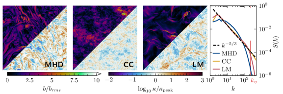
Figure 1: Slice plots of magnetic field strength $b/b_{rms}$ and logarithm of fieldline curvature $\kappa/\kappa_{\mathrm{peak}}$ for three models of magnetic turbulence — Magnetohydrodynamics (MHD), Continuous Cascade (CC) and Lagrangian Mapping (LM). Energy spectra of the models are plotted in the right-most panel and compared with a $-5/3$rd scaling. The dissipation wavenumber of the MHD simulation $k_{\eta}$ is indicated on the abscissa. The fieldline curvature is defined as $\kappa=\|\hat{\mathbf{b}}\cdot\nabla\hat{\mathbf{b}}\|$, with $\hat{\mathbf{b}}=\mathbf{b}/\|\mathbf{b}\|$, and normalized by the most frequent value $\kappa_{\mathrm{peak}}$.

Methods — We start by extending the continuous cascade in wavelet space [27] to three-dimensional divergence-free vector fields. The continuous cascade at scale $l$ and position $\mathbf{x}$ is represented by a log-infinitely divisible process $e^{\omega_{l}(\mathbf{x})}$, which gives the scale- and position-dependent intensity of a vector field $\mathbf{v}(\mathbf{x})$. This field is obtained by a vector-valued wavelet transform of $l^{H}e^{\omega_{l}}$ over the inertial range scales $l_{\mathrm{min}}<l<l_{0}$ as

$$\mathbf{v}(\mathbf{x})=\nabla\times A\int_{l_{\mathrm{min}}}^{l_{0}}l^{H-d-1}\big{(}e^{\omega_{l}}R_{l}\ast l{\psi}_{l}\hat{\mathbf{z}}\big{)}(\mathbf{x})\mathop{}\!\mathrm{d}{l}.$$ (1)

The slope of the energy spectrum is given by $-2H-1$, torodial wavelets $\nabla\times\big{(}l\psi_{l}(\mathbf{x})\hat{\mathbf{z}}\big{)}$ with $\psi(\mathbf{k})=-k^{2}e^{-k^{2}}$ and $\psi_{l}(\mathbf{x})=\psi(\mathbf{x}/l)$ ensure the zero-divergence condition $\nabla\cdot\mathbf{v}=0$, a random rotation field $R_{l}(\mathbf{x})$ with correlation length $l$ ensures proper isotropization of these wavelets, and the numerically determined constant $A$ normalizes the field to $\langle v^{2}\rangle=1$. Further, the curl can be moved in front of the spatial convolution operator $\big{(}f\ast\nabla\times g\big{)}(\mathbf{x})=\nabla\times\int_{\mathbb{R}^{3}}f(\mathbf{y})g(\mathbf{x}-\mathbf{y})\mathop{}\!\mathrm{d}{\mathbf{y}}$ and the scale integral $\int\cdots\mathop{}\!\mathrm{d}{l}$, thus allowing us to express the field in terms of a vector potential $\mathbf{v}=\nabla\times\mathbf{a}$.

The infinitely divisible process $\omega_{l}(\mathbf{x})$ is defined on cone-like subsets of the position-scale half-space $\mathbb{R}^{d}\times\mathbb{R}_{>0}$ equipped with the measure $l^{-d-1}\mathop{}\!\mathrm{d}{\mathbf{x}}\mathop{}\!\mathrm{d}{l}$ and has a cumulant generating function $\phi(q)$. Thus, the moments of the intensity process can be computed as $\langle e^{q\omega_{l}}\rangle=(l_{0}/l)^{c_{d}\phi(q)}\ \forall q\in\mathbb{N}$, where $c_{d}=2^{-d}\pi^{d/2}/\Gamma(d/2+1)$ comes from the scale-space cone volume. We consider a Gaussian distribution with $\phi(q)=\mu/2(p^{2}-p)$ with intermittency parameter $\mu$, in which case $e^{\omega_{l}}$ corresponds to the Gaussian multiplicative chaos employed by Pereira et al. [24] and related works.

As shown below, the vector field given by Equation (1) exhibits (isotropic) anomalous scaling, but lacks coherent features, so we introduce advective structures by adapting the minimal multiscale Lagrangian map (MMLM) [22, 23] to our framework. In short, the MMLM procedure considers only the advective part of the magnetic field evolution equation, i.e. $\left(\partial_{t}+\mathbf{u}\cdot\nabla\right)\mathbf{b}=0$, which can be solved at time $\tau$ with the Lagrangian ansatz $\mathbf{b}(\mathbf{x}_{\tau},\tau)=\mathbf{b}(\mathbf{x}_{0},0)$ and the linearized solution $\mathbf{x}_{\tau}=\mathbf{x}_{0}+\tau\mathbf{u}(\mathbf{x}_{0},0)$. Usually, two initially Gaussian random vector fields representing $\mathbf{u}(\mathbf{x})$ and $\mathbf{b}(\mathbf{x})$ are deformed on successively finer scales $l_{i}$ by applying the linearized Lagrangian solution with $\tau\propto l_{i}$ to the underlying regular grid, as described in the references.

In our framework, we first generate a random velocity field $\mathbf{u}(\mathbf{x})$ according to Equation (1) and accumulate the deformations of the grid $\mathbf{x}$ over all scales $l_{i}$ given by the discretization of the scale integral. Since our algorithm is formulated in terms of a vector potential, the Lagrangian step is computed with intermediate results $\mathbf{u}_{l_{i}}=\nabla\times\mathbf{a}_{l_{i}}^{\mathbf{u}}$. By using finite difference or Fourier methods to compute the curl, the velocity field $\mathbf{u}(\mathbf{x})$ remains unaffected by the deformed grid. We then generate an independent random magnetic vector potential $\mathbf{a}_{l_{\mathrm{min}}}^{\mathbf{b}}(\mathbf{x})$ with Equation (1) and evaluate it via inverse distance weighting at the deformed grid after the final step of the scale integral and before applying the curl. Thus, we are solving the advection equation for the magnetic vector potential

$$(\partial_{t}+\mathbf{u}\cdot\nabla)\,\mathbf{a}^{\mathbf{b}}_{l_{\mathrm{min}}}=0,$$ (2)

which is exact in two dimensions and making it especially suitable for strong guide field situations [41].

The deformation timescale $\tau=c\,l_{i}/\operatorname{max}(\|\mathbf{u}_{l_{i}}\|)$ is normalized to the maximal value of the current velocity magnitude and governed by the constant $c$. This constant is a free parameter, which must be chosen carefully, as it should be large enough for coherent structures to emerge, but not too large to avoid decorrelation. For higher values of $c$, energy accumulates on smaller scales, which is corrected by reweighting $\mathbf{a}^{\mathbf{b}}_{l_{\mathrm{min}}}(\mathbf{x})$ after interpolation with $k^{\delta/2}$, where $\delta$ is the deviation of the energy spectrum scaling from the expected $-5/3$rd scaling. Additionally, we mimic the effect of dissipation by applying a low-pass filter $\exp(-{k^{2}}/{2k_{0}^{2}})$.

For comparison, we perform a direct numerical simulation of incompressible resistive MHD turbulence in a three-dimensional periodic box with resolution $N^{3}=1024^{3}$, no background field and equal diffusivity and resistivity $\nu=\eta=1.2\times 10^{-3}$ [42]. The velocity is driven on Fourier modes $1\leq k\leq 3$ with the random forcing proposed by Alvelius [43], which exhibits very low mean cross-helicity and low noise in the time evolution of turbulence bulk quantities. For this purpose we employed the pseudo-spectral code SpecDyn, which was developed in the context of magnetic dynamo action and is tailored for use on modern HPC systems [44, 45].

Results — We generate sample fields of the continuous cascade process (CC) given by Equation (1) and its minimal multiscale Lagrangian mapping extension (LM) corresponding to Equation (2) on a three-dimensional periodic grid with resolution $N^{3}=1024^{3}$. The parameters of both processes are $H=1/3$, $l_{0}=0.5$ and $l_{\mathrm{min}}\approx 1.5\mathop{}\!\mathrm{d}{x}$. The intermittency parameter of the CC process is $\mu=0.4$, and the additional parameters of the LM process are $\mu=0.1$, $c=0.2$, $\delta=-0.45$, and $k_{0}=256$.

For visual inspection, slices of field strength and fieldline curvature are plotted in Figure 1, together with a plot of the radially averaged energy spectra. MHD turbulence is characterized by elongated and intricately intertwined coherent structures, while the CC field consists of incoherent intermittent “clouds” of large field strength values. The LM field exhibits thin and intense coherent structures, which are more spatially isolated. While CC and LM match the expected $-5/3$rd scaling rather well, the impact of resistivity of the MHD simulation becomes apparent.

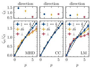
Figure 2: Scaling exponents of conditional structure functions of the magnetic field $\big{\langle}\big{(}\delta b_{\perp}\big{)}^{p}|\,\hat{\mathbf{d}}\,\big{\rangle}\propto d^{\zeta_{p}}$ for the MHD, CC and LM case. The averages of the increments $\delta{b}_{\perp}$ are conditional on the displacement vector $\mathbf{d}$ being aligned with the local mean field $\mathbf{b}_{\mathrm{local}}$ ($\parallel$), the normal fluctuation direction $\delta\hat{\mathbf{b}}_{\perp,N}\perp\hat{\mathbf{b}}_{\mathrm{local}}$ ($\delta\hat{\mathbf{b}}$), or with the binormal direction $\delta\hat{\mathbf{b}}_{\perp,N}\times\hat{\mathbf{b}}_{\mathrm{local}}$ ($\perp$). The scaling exponents are normalized as $\zeta_{p}/\zeta_{3}$ and the raw values of $\zeta_{3}$ are shown in the top panels.

We employ conditional structure functions [46] to study intermittency with respect to the local structure of the field. Given a displacement vector $\mathbf{d}$ at a point $\mathbf{X}$, we consider increments $\delta\mathbf{b}_{\perp}=\mathbf{b}_{\perp}(\mathbf{X}+\mathbf{d})-\mathbf{b}_{\perp}(\mathbf{X})$ perpendicular to the local mean field $\mathbf{b}_{\mathrm{local}}=\big{(}\mathbf{b}(\mathbf{X}+\mathbf{d})+\mathbf{b}(\mathbf{X})\big{)}/2$. Averages over these increments are taken conditionally on the direction of $\mathbf{d}$ in an instantaneous local basis given by $\hat{\mathbf{b}}_{\mathrm{local}}$, the normal direction of the fluctuations $\delta\hat{\mathbf{b}}_{\perp,N}$ with $\delta\mathbf{b}_{\perp,N}=\delta\mathbf{b}_{\perp}-\big{(}\delta\mathbf{b}_{\perp}\cdot\hat{\mathbf{b}}_{\mathrm{local}}\big{)}\hat{\mathbf{b}}_{\mathrm{local}}$ and the binormal direction $\hat{\mathbf{b}}_{\mathrm{local}}\times\delta\hat{\mathbf{b}}_{\perp,N}$. Based on this, the scaling exponents of the conditional averages $\big{\langle}\|\delta\mathbf{b}_{\perp}\|^{p}|\,\hat{\mathbf{d}}\,\big{\rangle}\propto d^{\zeta_{p}}$ are denoted as $\zeta_{p,\parallel}$, $\zeta_{p,\delta\hat{\mathbf{b}}}$ or $\zeta_{p,\perp}$ depending on $\mathbf{d}$ being aligned with $\hat{\mathbf{b}}_{\mathrm{local}}$, $\delta\hat{\mathbf{b}}_{\perp,N}$ or $\hat{\mathbf{b}}_{\mathrm{local}}\times\delta\hat{\mathbf{b}}_{\perp,N}$.

Figure 2 shows the normalized scaling exponents $\zeta_{p}/\zeta_{3}$ as well as the raw values of $\zeta_{3}$ for the three models and the three directions. The further $\zeta_{p}/\zeta_{3}$ deviates from the linear case, the more intermittent is the process, and smaller values of $\zeta_{3}$ correspond to a rougher process. In the MHD case, the direction parallel to the local mean field is the most smooth and non-intermittent, while the fluctuation and perpendicular direction are equally intermittent, the latter being the most rough. In contrast to this, the CC case shows no significant difference between the three directions, which are all equally rough and intermittent and which is expected from the lack of coherent structures. Lastly, the LM case exhibits again directional dependency, with parallel being the most non-intermittent and perpendicular the most intermittent. However, the fluctuation direction resembles more closely the parallel than the perpendicular direction.

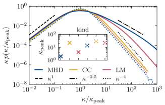
Figure 3: Compensated distributions of fieldline curvature $\kappa\,p(\kappa/\kappa_{\mathrm{peak}})$ for the MHD, CC and LM case, as well as their respective random-phase cases (dotted lines). The low-curvature $\kappa^{1}$ scaling, the MHD $\kappa^{-2.5}$ scaling and the Gaussian $\kappa^{-4}$ scaling are indicated for comparison. The inset shows the respective values of $\kappa_{\mathrm{peak}}$

While the conditional structure functions provide an extensive statistical picture of magnetic turbulence, additional geometric insight can be gained from the fieldline curvature

$$\kappa=\|\hat{\mathbf{b}}\cdot\nabla\hat{\mathbf{b}}\|=\|\hat{\mathbf{b}}\times(\mathbf{b}\cdot\nabla\mathbf{b})\|/\|\mathbf{b}\|^{2}.$$ (3)

Figure 3 shows the distributions $p(\kappa)$ for the three cases and their random-phase counterparts. The MHD case, in agreement with the literature [38, 39], behaves asymptotically as $p(\kappa)\underset{\kappa\to\infty}{\sim}\kappa^{-2.5}$. The CC case agrees, apart from being slightly wider, with the Gaussian random-phase fields, which scale distinctly as $p(\kappa)\underset{\kappa\to\infty}{\sim}\kappa^{-4}$. Finally, the LM case appears as an intermediate case between the previous two cases; its distribution function $p(\kappa)$ is slightly more narrow than the MHD case and around the slightly right-shifted peak, $p(\kappa)$ faintly resembles the $\kappa^{-2.5}$ scaling, before adjusting to the Gaussian $\kappa^{-4}$ scaling.

The extended flat tail for large $\kappa$ in the MHD case is caused by a significant amount of intermittent sharp fieldline bends scattered throughout the domain [see also 32, 33] and the low value of $\kappa_{\mathrm{peak}}$ comes from coherent structures extended on scales comparable to the box size. In contrast to this, fieldline bends in Gaussian fields are distributed in a self-similar way in the domain, thus leading to a much stepper decay of the distribution.

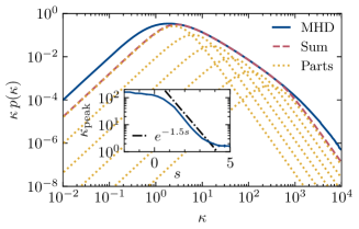
Figure 4: Modelling of the compensated MHD fieldline curvature distribution $\kappa\,p(\kappa)$ as a weighted sum of shifted Gaussian fieldline curvature distributions. The Gaussian fields have power-law spectra $S(k)\sim k^{-s}$, where the spectral slope $s$ determines the value of the most dominant curvature $\kappa_{\mathrm{peak}}$. The weights (not shown) scale analogously to the compensated high-curvature tail with $\kappa^{-1.5}$.

Since the random-phase fields are Gaussian random variables, their normalized fieldline curvature follows a universal distribution $p(\kappa/\kappa_{\mathrm{peak}})$, which is independent of the energy spectrum. However, $\kappa_{\mathrm{peak}}$ does depend on the energy spectrum, e.g. via the slope $s$ in case of a power-law spectrum $\sim k^{-s}$. Flatter spectra implicate more energy on small scales, resulting in more contributions from high curvatures and consequently larger $\kappa_{\mathrm{peak}}$. This connection is illustrated in Figures 4, where $p_{\mathrm{MHD}}(\kappa)$ is modeled as a weighted sum of Gaussian components, similar to the description of the turbulent velocity increment distribution function as a Gaussian scale mixture [47].

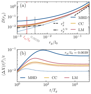
Figure 5: (a) Diffusion coefficients for gyro radii $r_{g}/l_{0}=0.001,\cdots,0.25$ for the MHD, CC and LM case, as well as their respective random-phase cases (dotted lines). High- and low-energy predictions from quasilinear theory are given for comparison. The dissipative length scale $l_{\eta}$ and the gyro radius of the example in the lower panel are indicated on the abscissa.
(b) Running diffusion coefficients of particles with gyro radius $r_{g}/l_{0}=0.0039$ as an example to illustrate the temporal evolution of the transport.

In addition to the insight into the structure of the fields gained by the previous steps, we also study the transport of charged particles by numerically solving test particle trajectories $\mathbf{X}(t)$ according to the Newton-Lorentz equation

$$\ddot{\mathbf{X}}(t)=l_{0}/r_{g}\,\dot{\mathbf{X}}(t)\times\mathbf{b}\big{(}\mathbf{X}(t)\big{)}$$ (4)

with a Boris integrator [48] and trilinear interpolation [49]. The magnetic field is normalized to ${\langle b^{2}\rangle}=1$ and the particles are parameterized by their normalized gyro radius $r_{g}/l_{0}=\gamma mcv_{0}/qb_{0}l_{0}$, where $l_{0}$ denotes the outer scale, $b_{0}$ denotes the root mean square strength of the magnetic field, and $v_{0}$, $\gamma=1/\sqrt{1-v^{2}/c^{2}}$, $m$ and $q$ denotes the particle’s velocity magnitude, Lorentz factor, mass and charge.

We record mean squared displacements $\langle\Delta X^{2}(t)\rangle=\langle\|\mathbf{X}(t)-\mathbf{X}(0)\|^{2}\rangle$ and diffusion coefficients $D(r_{g})=\lim_{t\to\infty}{\langle\Delta X^{2}(t)\rangle/t}$, once the trajectories have reached diffusive behaviour. The diffusion coefficients obtained from the three models are plotted in Figure 5a, and compared with their random-phase counterparts and quasi-linear predictions [10]. Figure 5b shows the exemplary time evolution of $\langle\Delta X^{2}(t)\rangle$ at $r_{g}/l_{0}=0.0039$, consisting of an initial super-diffusive phase and short sub-diffusive phase, before arriving at stable diffusive behaviour. Particles have the largest diffusion coefficients in MHD turbulence on all scales, which stands in striking difference to the random-phase MHD field, where we find the smallest diffusion coefficients. This behaviour can be explained by the strong deviation of the MHD energy spectrum at high wavenumbers from the $-5/3$rd spectral slope, and highlights impressively the effectiveness of coherent structures in regard to charged particle transport. The CC case achieves only a very minor increase compared to the random-phase case, and while the LM case performs better, it is still outperformed by MHD.

Conclusion — We have presented a novel algorithm for synthetic magnetic turbulence based on a combination of the continuous cascade model, generalized to three-dimensional divergence-free vector fields, and the minimal multiscale Lagrangian map. We compare this algorithm with an incompressible resistive MHD turbulence simulation and the pure three-dimensional continuous cascade model, which is intermittent but lacks coherent structures. This comparison is done by means of visual inspection, the energy spectrum, conditional structure function scaling, the fieldline curvature distribution and running diffusion coefficients of charged test particles.

We observe that our algorithm produces turbulence exhibiting pronounced coherent structures, albeit not as densely and intricately organized as MHD coherent structures. This is accompanied by non-trivial conditional structure function scaling, revealing local anisotropy, i.e. relatively low roughness ($\zeta_{3,\parallel}^{\mathrm{LM}}>\zeta_{3,\perp}^{\mathrm{LM}}$) and weak intermittency parallel to the local mean magnetic field, and strong intermittency in the perpendicular direction in agreement with MHD turbulence. However, when directly compared to the MHD case, the field in the parallel direction is clearly rougher ($\zeta_{3,\parallel}^{\mathrm{LM}}<\zeta_{3,\parallel}^{\mathrm{MHD}}$), and the fluctuation direction is not as intermittent as required. Further, the fieldline curvature distribution resembles the MHD case at small and intermediate curvatures, but exhibits Gaussian scaling at large curvatures. Finally, while charged particle transport is enhanced, it remains outpaced by the MHD case, as expected due to the simpler geometry and smaller length scales of the synthetic coherent structures.

In conclusion, our algorithm presents significant progress towards simulating realistic turbulence. Remaining issues are clearly identified and will guide further improvements in designing synthetic turbulence models. For instance, a feedback mechanism during the algorithm would be highly relevant, which acts on the velocity field $\mathbf{u}$ and takes the current state of the deformed grid and the advected magnetic field $\mathbf{b}$ into account. An approach based on the Elsässer formulation of the MHD equations appears promising as well. Alternatively, one could aim to design a synthetic scalar curvature field, instead of a full vector field, and make use of recent results linking fieldline curvature and charged particle transport [32, 33]. Such an approach could build on the description of the non-trivial MHD fieldline curvature distribution as a weighted sum of Gaussian components, as presented in this letter.

Supplementary Material: Towards Synthetic Magnetic Turbulence with Coherent Structures

The pseudocode for the algorithm described in the main text is listed in Algorithm 1.

Algorithm 1 Continuous Cascade/Lagrangian Map

function ContinuousCascade3D(DoLagrangianMap)

      $\triangleright$ arrays for inifinitely divisible intensity process, vector potential, grid coordinates

      allocate $\omega[\mathbf{x}]$, $\mathbf{a}[\mathbf{x}]$, $\mathbf{c}[\mathbf{x}]$

      for $i=0;\,i<n;\,i\leftarrow i+1$ do

          $\triangleright$ current scale, scale increment, scale-dependent variance of Gaussian noise

          $l_{i}\leftarrow l_{\mathrm{min}}(l_{0}/l_{\mathrm{min}})^{(n-i)/n}$

          $\Delta l\leftarrow l_{i}-l_{i+1}$

          $\sigma^{2}\leftarrow c_{d}\,\mu\,\Delta x^{d}\,\Delta l\,l_{i}^{-d-1}$

          $\triangleright$ sample next level of detail of the infinitely divisible intensity process

          sample $\Omega{[\mathbf{x}]}\sim\mathcal{N}(-\sigma^{2}/2,\sigma^{2}\Sigma_{l_{i}})$

          $\omega\leftarrow\omega+\Omega$

          $\triangleright$ sample parametrization of rotation matrix $R_{l}$

          sample $\cos\theta{[\mathbf{x}]}\sim\mathcal{U}(-1,1;\Sigma_{l_{i}})$

          sample $\phi{[\mathbf{x}]}\sim\mathcal{U}(0,2\pi;\Sigma_{l_{i}})$

          $\triangleright$ current step of scale integral

          ${a}_{{x}}\leftarrow{a}_{{x}}+\Delta l\,l_{i}^{H-d}(e^{\omega}\sin\theta\cos\phi\ast\psi_{l_{i}})$

          ${a}_{{y}}\leftarrow{a}_{{y}}+\Delta l\,l_{i}^{H-d}(e^{\omega}\sin\theta\sin\phi\ast\psi_{l_{i}})$

          ${a}_{{z}}\leftarrow{a}_{{z}}+\Delta l\,l_{i}^{H-d}(e^{\omega}\cos\theta\ast\psi_{l_{i}})$

          if DoLagrangianMap then

               $\triangleright$ compute intermediate vector field and advect grid coordinates

               $\mathbf{v}\leftarrow\nabla\times\mathbf{a}$

               $\mathbf{c}\leftarrow\mathbf{c}+c\,l_{i}\,\mathbf{v}/\mathtt{max}(\|\mathbf{v}\|)$

         end if

     end for

      if DoLagrangianMap then

          $\triangleright$ return advected grid coordinates

          return $\mathbf{c}$

      else

          $\triangleright$ return raw vector potential

          return $\mathbf{a}$

     end if

end function

function LagrangianMap3D

      $\triangleright$ sample advected grid coordinates

      $\mathbf{c}\leftarrow$ ContinuousCascade3D(true)

      $\triangleright$ sample independent vector potential

      $\mathbf{a}\leftarrow$ ContinuousCascade3D(false)

      $\triangleright$ interpolate vector potential onto regular grid by inverse distance weighting

      $\mathbf{a}\leftarrow\mathtt{idw}(\mathbf{a},\mathbf{c})$

      $\triangleright$ correct spectral slope and mimic dissipation

      $\mathbf{a}\leftarrow\mathtt{filter}(\mathbf{a},k^{\delta/2}e^{-(k/k_{0})^{2}/2})$

      $\triangleright$ compute curl

      $\mathbf{b}\leftarrow\nabla\times\mathbf{a}$

      $\triangleright$ return normalized vector field

      return $\mathbf{b}/\sqrt{\langle\mathbf{b}^{2}\rangle}$

end function

The function ContinuousCascade3D generates a sample of the vector field process

$$\mathbf{v}(\mathbf{x})=\nabla\times A\int_{l_{\mathrm{min}}}^{l_{0}}l^{H-d}\big{(}e^{\omega_{l}}R_{l}\ast{\psi}_{l}\hat{\mathbf{z}}\big{)}(\mathbf{x})\mathop{}\!\mathrm{d}{l},$$ (5)

by discretizing the scale integral $\int\cdots\mathop{}\!\mathrm{d}{l}$ with a geometric progression. If requested, after each step of the scale integral, the curl of the intermediate result is computed to linearly advect the grid coordinates $\mathbf{c}(\mathbf{x})$, as described in the main text.

The basis wavelet is defined in Fourier space as $\psi(\mathbf{k})=-k^{2}e^{-k^{2}}$ and rescaled in real space as $\psi_{l}(\mathbf{x})=\psi(\mathbf{x}/l)$. The Gaussian infinitely divisible intensity process $\omega_{l}(\mathbf{x})$ is sampled as a sum of successively finer details $\Omega_{l}(\mathbf{x})\sim\mathcal{N}(-\sigma_{l}^{2}/2,\sigma_{l}^{2}\Sigma_{l})$, which are Gaussian random scalar fields with correlation length $l$ as indicated by a correlation matrix $\Sigma_{l}$. Such a field can be easily sampled by convolving uncorrelated standard Gaussian noise with a mollifier with width $l$, scaling to the given variance and shifting to the given mean.

For proper isotropization, the wavelets $\psi_{l}(\mathbf{x})\hat{\mathbf{z}}$ are rotated by an angle $\theta_{l}$ around an axis $\hat{\mathbf{w}}_{l}=(\cos\phi_{l},\sin\phi_{l},0)$, summarized by the rotation matrix

$$R_{l}=\begin{pmatrix}\ast&\ast&\sin\theta_{l}\cos\phi_{l}\\ \ast&\ast&\sin\theta_{l}\sin\phi_{l}\\ \ast&\ast&\cos\theta_{l}\end{pmatrix},$$ (6)

where only the third column is relevant when applied to the vector $\psi_{l}\hat{\mathbf{z}}$. The angles $\cos\theta_{l}\sim\mathcal{U}(-1,1;\Sigma_{l})$ and $\phi_{l}\sim\mathcal{U}(0,2\pi;\Sigma_{l})$ are random fields with uniform distributions and correlation length $l$ as indicated by a correlation matrix $\Sigma_{l}$. These fields are sampled by first sampling uncorrelated standard Gaussian noise from $\mathcal{N}(0,\mathbb{I})$, convolving with a mollifier with width $l$, and applying the Gaussian cumulative distribution function $\Phi(x)=\frac{1}{2}\left(1+\operatorname{erf}\frac{x}{\sqrt{2}}\right)$ to obtain uniformly distributed random variables. Finally, the fields are shifted to their desired intervals.

The function LagrangianMap3D samples a vector field and the associated advected coordinates $\mathbf{c}$ by calling ContinuousCascade3D(true), and a second independent vector potential $\mathbf{a}(\mathbf{x})$ by calling ContinuousCascade3D(false). This can either be done in parallel or sequentially, potentially overwriting the first vector potential if memory is limited. The second vector field is interpreted as being transported by the first one, which is expressed by writing $\mathbf{a}(\mathbf{c})$.

Then, $\mathbf{a}$ is interpolated from the deformed grid $\mathbf{c}$ back onto the regular grid $\mathbf{x}$ by (pruned) inverse distance weighting, i.e. all contributions from grid points $\mathbf{c}_{k}$ within a radius $2\mathop{}\!\mathrm{d}{x}$ around grid point $\mathbf{x}_{j}$ are collected and weighted by their inverse distance, as

$$\mathbf{a}(\mathbf{x}_{j})=\frac{\displaystyle\sum_{\mathbf{c}_{k},\|\mathbf{c}_{k}-\mathbf{x}_{j}\|<2\mathop{}\!\mathrm{d}{x}}w(\mathbf{x}_{j},\mathbf{c}_{k})\,\mathbf{a}(\mathbf{c}_{k})}{\displaystyle\sum_{\mathbf{c}_{k},\|\mathbf{c}_{k}-\mathbf{x}_{j}\|<2\mathop{}\!\mathrm{d}{x}}w(\mathbf{x}_{j},\mathbf{c}_{k})},$$ (7)

with weights $w(\mathbf{x}_{j},\mathbf{c}_{k})=\|\mathbf{x}_{j}-\mathbf{c}_{k}\|_{\varepsilon}^{-1}$ and a regularized metric $\|\mathbf{v}\|^{2}_{\varepsilon}=\|\mathbf{v}\|^{2}+\varepsilon^{2}$ for small $\varepsilon$.

Additional reweighting in Fourier space to correct the spectral slope and to mimic dissipation is done as described in the main text.