Testing the consistency of early and late cosmological parameters with BAO and CMB data

Abstract

The recent local measurements of the Hubble constant $H_{0}$, indicate a significant discrepancy of over 5$\sigma$ compared to the value inferred from Planck observations of the cosmic microwave background (CMB). In this paper, we try to understand the origin of this tension by testing the consistency of early and late cosmological parameters in the same observed data. In practice, we simultaneously derive the early and late parameters using baryon acoustic oscillation (BAO) measurements, which provide both low and high-redshift information. To resolve parameter degeneracy, the complementary data from CMB observations are included in the analysis. By using the parameter $\omega_{m}=\Omega_{m}h^{2}$, we introduce ${\rm ratio}(\omega_{m})$, defined as the ratio of $\omega_{m}$ which are constrained from high and low-redshift measurements respectively, to quantify the consistency between early and late parameters. We obtained a value of ${\rm ratio}(\omega_{m})=1.0069\pm 0.0070$, indicating there is no tension between early parameters and late parameters in the framework of $\Lambda$CDM model. As a result, the Hubble tension may arise from the differences of datasets or unknown systematic errors in the current data. In addition, we forecast the future BAO measurements of ${\rm ratio}(\omega_{m})$, using several galaxy redshift surveys and 21 cm intensity mapping surveys, and find that these measurements can significantly improve the precision of cosmological parameters.

I Introduction

The standard cosmological model, $\Lambda$CDM, has withstood the rigorous scrutiny due to significant advances in observations of the cosmic microwave background (CMB) Aghanim et al. (2020); Balkenhol et al. (2021); Aiola et al. (2020), Type Ia supernovae (SNIa) Scolnic et al. (2018); Brout et al. (2022) and large-scale structure Alam et al. (2017, 2021); Abbott et al. (2018) in recent years. However, tensions have emerged for several parameters when they are inferred from distinct observations within the $\Lambda$CDM. The most significant tension is related to determinations of the Hubble constant $H_{0}$. The representative difference is between the SH0ES Riess et al. (2022) determination of $H_{0}$ and the value inferred from Planck Aghanim et al. (2020) for the $\Lambda$CDM cosmology, which has increased to $5\sigma$ level Verde et al. (2019); Abdalla et al. (2022a). Actually, the tension exists in not only these two values, but also in two sets of measurements Abdalla et al. (2022a).

One set contains indirect estimates at early times which are cosmological model dependent, such as CMB and Baryon Acoustic Oscillation (BAO) Cuceu et al. (2019); Schöneberg et al. (2022). As mentioned above, the Planck 2018 release Aghanim et al. (2020) predicts $H_{0}=67.36\pm 0.54\ \rm km\ s^{-1}\ Mpc^{-1}$ in combination with the CMB lensing. Moreover, the final combination of the BAO measurements from galaxies, quasars, and Lyman-$\alpha$ forest (Ly-$\alpha$) from Baryon Oscillation Spectroscopic Survey (BOSS) prefers $H_{0}=67.64^{+0.94}_{-1.03}\ \rm km\ s^{-1}\ Mpc^{-1}$ Schöneberg et al. (2022) involving a prior on the physical density of the baryons $\Omega_{b}h^{2}$ derived from the latest Big Bang Nucleosynthesis (BBN) measurements of the primordial deuterium Cooke et al. (2018); Mossa et al. (2020). In contrast, another set includes direct late time cosmological model-independent measurements, such as distance ladders Riess et al. (2022); Jang and Lee (2017); Freedman et al. (2020); Huang et al. (2020); Kourkchi et al. (2020); Santos et al. (2017) and strong lensing Wong et al. (2020). The determination of $H_{0}$ is based on calibration of the SNIa using the Cepheids, Miras and Tip of the Red Giant Branch (TRGB), which prefers a higher value. The latest SH0ES measurement gives $H_{0}=73.04\pm 1.04\ \rm km\ s^{-1}\ Mpc^{-1}$ using Cepheid period–luminosity relations to calibrate distances to Type Ia SNe host galaxies Riess et al. (2022).

There are various potential solutions proposed for the Hubble tension. One kind of viewpoint thinks that some unknown systematic errors affect either early-universe or late-universe observation Di Valentino et al. (2021). However, the other viewpoint is related to the new physics beyond the standard cosmological model. The late time modifications of the $\Lambda$CDM expansion history have been showed that they cannot resolve the Hubble tension through a model independent method in Lemos et al. (2019); Efstathiou (2021). Therefore, many solutions to the Hubble tension is to introduce new physics about early universe that increases the value of the Hubble constant inferred from the CMB. An popular early-time resolution Karwal and Kamionkowski (2016); Mörtsell and Dhawan (2018); Poulin et al. (2019) is an exotic early dark energy (EDE) that behaves like a cosmological constant at early time and dilutes faster than radiation at later time. It addresses the Hubble tension by decreasing the sound horizon while leaving the later evolution of the Universe unchanged.

In order to understand the Hubble tension, it is important to ask the question: Whether or not the inconsistency of the cosmological parameter exists in the same observed data? In this paper, we achieve the simultaneous constraints on the early and late cosmological parameters with the help of BAO measurements that contain both low and high-redshift universe information. This approach enables us to investigate if any tension exists between early and late epochs within the $\Lambda$CDM cosmology. If the Hubble tension is caused by the new physics beyond $\Lambda$CDM model, in principle we should discover the different values of $H_{0}$ from only early and only late information of BAO data. However, if this kind of difference is not discovered, as we present in this article, it would prefer to the solution of Hubble tension with some unsolved systematics in the cosmological measurement. In practice, two distinct $\Lambda$CDM cosmological parameter sets are employed to construct the expansion history of the early and late universe separately. However, due to the degeneracy, CMB data is combined with BAO data for breaking it and $H_{0}$ is replaced by a new parameter ${\rm ratio}(\omega_{m})$, which will be introduced detail in Section II. This new parameter can help us test the consistency of cosmological parameters and determine the origin of the Hubble tension. As a result, we find no evidence of new physics beyond $\Lambda$CDM cosmology.

This article is organized as follows. In Section II, we introduce the methods and datasets used in this analysis. The results and related discussions are presented in Section III. We simulate future BAO experiments and analyze the results in Section IV. Finally, Section V presents our conclusions in this article.

II Methodology

In the standard Friedmann-Lemaitre-Robertson-Walker (FLRW) universe, the Hubble parameter $H(z)$ on the basis of flat $\Lambda$CDM is given by:

$$H(z)=H_{0}\sqrt{{\Omega}_{r}(1+z)^{4}+{\Omega}_{m}(1+z)^{3}+{\Omega}_{\Lambda}},$$ (1)

where ${\Omega}_{r}$, ${\Omega}_{m}$ and ${\Omega}_{\Lambda}$ are the fractional densities of radiation, matter and dark energy at redshift $z=0$ and constrained by ${\Omega}_{r}+{\Omega}_{m}+{\Omega}_{\Lambda}=1$.

As previously indicated regarding the Hubble tension, the 5$\sigma$ difference between early time and late time inspires us to investigate whether its reason is physical. In practice, the BAO data which contains both low and high-redshift universe information will be analyzed in the framework of the flat $\Lambda$CDM cosmology. We employ two distinct independent cosmological parameter sets to describe the expansion history of the early and late universe separately. Therefore, the consistency of these two cosmological parameter sets can help us distinguish the cause of the Hubble tension. In order to realize it, the parameters in the standard cosmological model can be generalized as follows:

1. Parameter set undergoes a transition from
   $\{H_{0},\Omega_{m}\}$ to $\{\tilde{H}_{0},\tilde{\Omega}_{m},H_{0},\Omega_{m}\}$. Note that, here and afterwards, the parameters with tilde label that their values are derived from early cosmological information and we call them as “early cosmological parameters” in this article, while the parameter without tilde label that their values are derived from late cosmological information and we call them as “late cosmological parameters”.

2. Recombination redshift $z_{*}$ serves as the dividing line between the early and late universe. Namely the early parameters $\left(\tilde{H}_{0},\tilde{\Omega}_{m}\right)$ are determined from the measurements whose redshift is larger than the recombination redshift $z_{*}$, while the late parameters remain similar. Therefore we realize constructing the early and late expanding history of the Universe individually.

3. In order to test $\Lambda$CDM model through the constraint of both early and late parameters simultaneously, we can compare whether early parameters $\left(\tilde{H}_{0},\tilde{\Omega}_{m}\right)$ and $\left(H_{0},\Omega_{m}\right)$ are consistent. We are able to determine whether the tension between early and late parameters of $\Lambda$CDM exists by the combination of BAO and CMB data.

More details will be discussed in the data analysis part.

II.1 BAO data

In the primordial plasma of the early universe, photon-matter interactions give rise to substantial heat and outward pressure. This pressure drives baryons and photons out of the overdensity area at a speed of sound $c_{s}$. As a result, the spherical sound waves propagate baryon density fluctuations in the Universe until the recombination epoch. The distance traveled by sound waves between the end of inflation and the decoupling of baryons from photons after recombination is referred to as the sound horizon $r_{s}$. Dark matter remains at the center of acoustic wave since it is influenced solely by gravity. Finally, the baryons and dark matter resulted in a structure that included matter overdensities both at the original site and at the sound horizon scale. Thus, we can anticipate observing a more significant number of galaxy pairs separated by the sound horizon distance than other length scales. In other words, the BAO method relies on the imprint left by propagation of acoustic density waves to provide a cosmic standard ruler which has a comoving scale $r_{s}$.

The comoving sound horizon $r_{s}(z)$ is given by Eisenstein and Hu (1998):

$$r_{s}(z)=\frac{c}{H_{0}}\int_{z}^{\infty}\frac{c_{s}}{E(z^{\prime})}\mathrm{d}z^{\prime},$$ (2)

where $c$ is the speed of light, $H_{0}=100h\rm\ km\ s^{-1}Mpc^{-1}$ with $h$ the dimensionless Hubble constant, the sound speed is $c_{s}=1/\sqrt{3(1+R_{b}a)}$, with $R_{b}a=3\rho_{b}/(4\rho_{r})$, and $R_{b}=31500\omega_{b}(T_{CMB}/2.7K)^{-4}$ with $\omega_{b}=\Omega_{b}h^{2}$ and the CMB temperature $T_{CMB}=2.7255K$. It is necessary to emphasize that the radiation component cannot be ignored when calculating the comoving sound horizon $r_{s}$. It can be described by the matter fraction $\omega_{m}$ applying matter-radiation equality relation $\Omega_{r}=\Omega_{m}/(1+z_{eq})$, and $z_{eq}=2.5\times 10^{4}\omega_{m}(T_{CMB}/2.7K)^{-4}$, where $\omega_{m}=\Omega_{m}h^{2}$.

The BAO feature appears in both the line-of-sight direction and the transverse direction and provides a measurement of $D_{H}(z)/r_{d}$ and $D_{M}(z)/r_{d}$ individually:

$$\frac{D_{H}(z)}{r_{d}} = \frac{c}{H(z)r_{d}},$$ (3)

$$\frac{D_{M}(z)}{r_{d}} = \frac{c}{H_{0}r_{d}}\Gamma(z),$$ (4)

where $r_{d}$ is the sound horizon at the drag epoch $r_{s}(z_{d})$ and $D_{M}$ is the same as transverse comoving distance Hogg (1999). The transverse comoving distance, which depends on FLRW metric to an object at redshift $z$, is given by

$$D_{M}(z)=r(z)=\frac{c}{H_{0}}S_{k}(\Gamma(z)),$$ (5)

where $\Gamma(z)=\int_{0}^{z}{\mathrm{d}z^{\prime}}/{E(z^{\prime})}$, $E(z)=H(z)/H_{0}$. Note that the angular diameter distance $D_{A}(z)$ has relation with the comoving angular diameter distance $r(z)$: $D_{A}(z)=r(z)/(1+z)$. Because $S_{k}(x)=x$ for flat $\Lambda$CDM model, we have $r(z)=c\Gamma(z)/H_{0}$ in the following analysis.

The BAO measurements were also historically summarized by a single quantity representing the spherically averaged distance

$$D_{V}(z)\equiv[zD_{M}^{2}(z)D_{H}(z)]^{1/3}.$$ (6)

The redshift of the drag epoch can be approximated as Hu and Sugiyama (1996)

$$z_{d}=\frac{1345\omega_{m}^{0.251}}{1+0.659\omega_{m}^{0.828}}[1+b_{1}\omega_{b}^{b_{2}}],$$ (7)

where

$$b_{1}=0.313\omega_{m}^{-0.419}[1+0.607\omega_{m}^{0.674}],b_{2}=0.238\omega_{m}^{0.223}.$$ (8)

It is obvious that BAO measurements provide simultaneous information about the early and late universe through the comoving sound horizon $r_{d}$ and Hubble parameter $H(z)$, which enables us to determine the physics in the early and late universe simultaneously.

To calculate the sound horizon $r_{d}$ and complete the set of cosmological parameters, we must also include information on baryon density $\Omega_{b}$ as an early parameter not only because it derives from CMB observation, but also it is just entailed to compute sound horizon $r_{d}$. Carrying over the remaining parameters introduced above, the initial full parameter set is now:

$$\centering\{\tilde{\Omega}_{b},\tilde{\Omega}_{m},\tilde{H}_{0},\Omega_{m},H_{0}\}.\@add@centering$$

Then, the BAO measurements can be expressed in this parameter set:

$$\frac{D_{H}(z)}{r_{d}}=\frac{\left[(1+z)^{3}+\Omega_{l}-1\right]^{-\frac{1}{2}}}{\int_{z_{d}}^{\infty}\left[3\left(1+\frac{R_{b}}{1+z^{\prime}}\right)(1+z^{\prime})^{3}f(\tilde{\omega}_{m},\omega_{m})\right]^{-\frac{1}{2}}\mathrm{d}z^{\prime}},$$ (9)

where $\Omega_{l}\equiv 1/\Omega_{m}$, and

$$f(\tilde{\omega}_{m},\omega_{m})\equiv\frac{\tilde{\omega}_{m}}{\omega_{m}}\left(1+\frac{1+z}{1+z_{eq}}\right).$$ (10)

The Hubble constant $H_{0}$ and matter density fraction $\Omega_{m}$ are fully degenerate with the form $\omega_{m}$. We can also find in Eq.(10) the ratio of $\omega_{m}$ is degenerate with the late cosmological parameter $\omega_{m}$ in the form of a sum due to $z_{eq}\propto\tilde{\omega}_{m}$. We will see the CMB data can break this degenerate relation in the next section. In addition, constraining this ratio help us compare the early and late cosmological parameters directly. Therefore, we introduce ${\rm ratio}(\omega_{m})\equiv\tilde{\omega}_{m}/\omega_{m}$ as a new parameter. The analysis of transverse measurement $D_{M}(z)/r_{d}$ is similar to $D_{H}(z)/r_{d}$.

The BAO measurements used in this work are taken from the 6dF Galaxy Survey (6dFGS,Beutler et al. (2011)), the complete Sloan Digital Sky Survey (SDSS) data release, including SDSS-Main Galaxy Sample (MGS,Ross et al. (2015)), the BOSS and the extended Baryon Oscillation Spectroscopic Survey (eBOSS) DR16 data Alam et al. (2021); Des Bourboux et al. (2020). A specific description of BAO data is shown in TABLE 1.

The likelihood of BAO $\mathcal{L}_{BAO}$ have different forms for different datasets. The covariance matrix of SDSS DR12 and eBOSS Quasar data, and the full (non-Gaussian) likelihoods for the Ly$\alpha$ forest data Des Bourboux et al. (2020) and emission line galaxies (ELG) analysis De Mattia et al. (2021), are from the public SDSS repository.

$z_{eff}$	Measured Quantity	Value	Dataset	Reference
0.106	$r_{d}/D_{V}$	$0.336\pm 0.015$	6dFGS	Beutler et al. (2011)
0.15	$D_{V}/r_{d}$	$4.47\pm 0.17$	SDSS DR7	Ross et al. (2015)
0.38	$D_{H}/r_{d}$	$25.00\pm 0.76$	SDSS DR12	Alam et al. (2021)
0.38	$D_{M}/r_{d}$	$10.23\pm 0.17$	SDSS DR12	Alam et al. (2021)
0.51	$D_{H}/r_{d}$	$22.33\pm 0.58$	SDSS DR12	Alam et al. (2021)
0.51	$D_{M}/r_{d}$	$13.36\pm 0.21$	SDSS DR12	Alam et al. (2021)
0.70	$D_{H}/r_{d}$	$19.33\pm 0.53$	eBOSS LRG	Alam et al. (2021)
0.70	$D_{M}/r_{d}$	$17.86\pm 0.33$	eBOSS LRG	Alam et al. (2021)
0.85	$D_{V}/r_{d}$	$18.33^{+0.57}_{-0.62}$	eBOSS ELG	Alam et al. (2021)
1.48	$D_{H}/r_{d}$	$13.26\pm 0.55$	eBOSS Quasar	Alam et al. (2021)
1.48	$D_{M}/r_{d}$	$30.69\pm 0.80$	eBOSS Quasar	Alam et al. (2021)
2.33	$D_{H}/r_{d}$	$8.93\pm 0.28$	eBOSS Ly$\alpha\times$ Ly$\alpha$	Des Bourboux et al. (2020)
2.33	$D_{M}/r_{d}$	$37.6\pm 1.9$	eBOSS Ly$\alpha\times$ Ly$\alpha$	Des Bourboux et al. (2020)
2.33	$D_{H}/r_{d}$	$9.08\pm 0.34$	eBOSS Ly$\alpha\times$ Quasar	Des Bourboux et al. (2020)
2.33	$D_{M}/r_{d}$	$37.3\pm 1.7$	eBOSS Ly$\alpha\times$ Quasar	Des Bourboux et al. (2020)

Table 1: Datasets measuring the BAO peak that are used in our cosmological analysis.

II.2 CMB data

CMB observation contribution in the constraint of cosmological parameter can be converted to CMB shift parameters for breaking degeneracy of parameters, instead of using the full CMB power spectrumWang and Mukherjee (2007); Wang and Wang (2013):

$$R = \sqrt{\Omega_{m}H^{2}_{0}}r(z_{*})/c,$$ (11)

$$l_{a} = \pi r(z_{*})/r_{s}(z_{*}).$$ (12)

These parameters can be considered as the CMB measurements which are extracted from CMB likelihood, where $z_{*}$ is the redshift of recombination. The sufficient information of Planck data release Aghanim et al. (2020) for constraint is given by CMB shift parameters with baryon density $\omega_{b}=\Omega_{b}h^{2}$.

The redshift $z_{*}$ can be calculated by the fitting formula Hu and Sugiyama (1996):

$$z_{*}=1048[1+0.00124\omega^{-0.738}_{b}][1+g_{1}\omega^{g_{2}}_{m}],$$ (13)

where

$$g_{1}=\frac{0.0783\omega^{-0.238}_{b}}{1+39.5\omega^{0.763}_{b}},g_{2}=\frac{0.560}{1+21.1\omega^{1.81}_{b}}.$$ (14)

The final result, which is extracted from Planck 2018 TT,TE,EE+lowE chains, can be transformed in terms of a data vector $\bm{v}=(R,l_{a},\omega_{b})^{T}$ and their covariance matrix. For a flat universe Zhai and Wang (2019), this data vector is

$$\bm{v}=\begin{pmatrix}1.74963\\ 301.80845\\ 0.02237\\ \end{pmatrix}$$ (15)

and the covariance matrix is

$$\bm{C_{v}}=10^{-8}\times\begin{pmatrix}1598.9554&17112.007&-36.311179\\ 17112.007&811208.45&-494.79813\\ -36.311179&-494.79813&2.1242182\end{pmatrix}$$

The compression of CMB data forms the so-called distance priors Wang and Mukherjee (2007), which can help us break the degeneracy of the BAO data:

$$l_{a}=\frac{\pi R}{\int_{z_{*}}^{\infty}\left[3\left(1+\frac{R_{b}}{1+z^{\prime}}\right)(1+z^{\prime})^{3}\left(1+\frac{1+z^{\prime}}{1+z_{eq}}\right)\right]^{-\frac{1}{2}}\mathrm{d}z^{\prime}}.$$ (16)

Apparently, $\tilde{\omega}_{m}$ is the only cosmological parameter to be determined in the CMB shift parameter $l_{a}$. Namely, combining the CMB data can give a constraint on $\tilde{\omega}_{m}$ and break the degeneracy to release ${\rm ratio}(\omega_{m})$. Therefore the final parameter set is now

$$\centering\{\tilde{\omega}_{b},\tilde{\omega}_{m},\Omega_{l},{\rm ratio}(\omega_{m})\}.\@add@centering$$

In summary, the baryon density $\tilde{\omega}_{b}$ and the matter density $\tilde{\omega}_{m}$ serve as early parameters to compute sound horizon $r_{s}$. $\Omega_{l}$ describes the evolution of late universe and ${\rm ratio}(\omega_{m})$ is a bridge between them.

The loglikelihood function for CMB can be written in the form:

$$\mathcal{L}_{CMB}=-\frac{1}{2}\chi^{2}_{CMB}=-\frac{1}{2}(\bm{v}-\bm{v}_{th})^{T}\bm{C_{v}}^{-1}(\bm{v}-\bm{v}_{th}),$$ (17)

and the complete likelihood for our cosmological analysis is the following $\mathcal{L}=\mathcal{L}_{\rm CMB}+\mathcal{L}_{\rm BAO}$. We run a Markov Chain Monte Carlo (MCMC) with the sampler emcee Foreman-Mackey et al. (2013) to constrain parameters, where the priors chosen for our Bayesian calculations regarding the cosmological parameters are uniform distributions: $\tilde{\omega}_{b}\in(0.001,0.3)$, $\tilde{\omega}_{m}\in(0.05,0.5)$, $\Omega_{l}\in(1,10)$, ${\rm ratio}(\omega_{m})\in(0.1,10)$.

III Results and Discussion

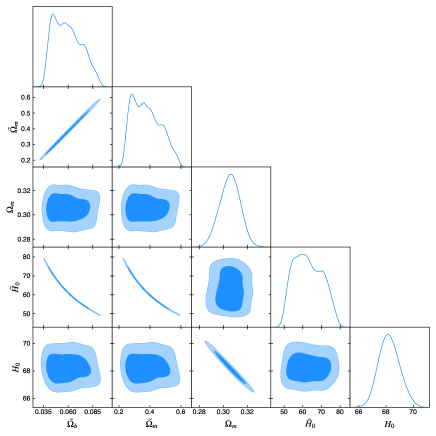
(a)

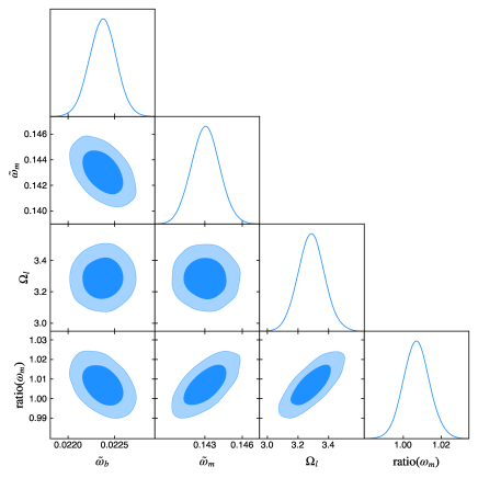
(b)

Figure 1: Posterior likelihoods (68% and 95% confidence level) for the initial parameter set (a) and final parameter set (b) considering the full samples of CMB and BAO.

The limitations of the parameters using BAO+CMB are illustrated in FIG.1, and the results are also summarized in TABLE 2. Notably, the parameters of initial set show complex degeneracy compared to those of the final set, particularly for early parameters such as $\tilde{\Omega}_{b}$, $\tilde{\Omega}_{m}$ and $\tilde{H}_{0}$. The fundamental reason for the degeneracy was elaborated in the previous section.

Parameters	Value
$\tilde{\omega}_{b}$	$0.02237\pm 0.00014$
$\tilde{\omega}_{m}$	$0.1430\pm 0.0011$
$\Omega_{l}$	$3.287\pm 0.087$
${\rm ratio}(\omega_{m})$	$1.0069\pm 0.0070$

Table 2: Cosmological constraints on early and late parameters simultaneously.

III.1 Comparison with separate constraints

There are early parameters and late parameters incorporated in our model, enabling the simultaneous constraint of both. Note that, there are substantial cosmological parameters estimations obtained from high-redshift or low-redshift data alone. Therefore, we firstly compare the results presented in this paper with other results which are constrained separately before discussing on the ${\rm ratio}(\omega_{m})$ and cosmological models.

Initially, we concentrate on the physical density of the early universe, denoted by $\tilde{\omega}_{m}=0.1430\pm 0.0011$. Another recent estimation of early cosmological parameters from CMB observations almost independently of the late-time evolution yields $\tilde{\omega}_{m}=0.1414\pm 0.0013$ Lemos and Lewis (2023). They accomplish it by constructing a CMB likelihood that does not require a cosmological model to model the late-time effects. This indicates that the estimation of early parameters obtained independently is consistent with the simultaneous constraint.

In contrast of degeneracy of early parameters, we can analyze late parameters $H_{0}$ and $\Omega_{m}$ individually. Their posteriors are derived from $\tilde{\omega}_{m}$, $\Omega_{l}$ and ${\rm ratio}(\omega_{m})$ showed in TABLE 2, and given by

$$H_{0} = 68.34\pm 0.97\rm\ km\ s^{-1}Mpc^{-1},$$

$$\Omega_{m} = 0.3042\pm 0.0081.$$ (18)

We can compare them with these values constrained by low-redshift observations, such as Supernovae. At first, we concentrate on the matter density $\Omega_{m}$ and adopt $\Omega_{m}=0.298\pm 0.022$ from the Pantheon analysis Scolnic et al. (2018). It is apparent that the Pantheon result is in agreement with ours. We also notice that constraint of $\Omega_{m}$ in this work is tighter than the result Pogosian et al. (2020) $\Omega_{m}=0.294^{+0.014}_{-0.016}$ constrained by BAO with a prior of $\omega_{m}$.

We divide the BAO measurements into early and late portions to limit the value of the Hubble constant, $H_{0}$, using information from the late universe. Therefore it is interesting that compare it with $H_{0}$ measurements which are derived from local observation of SNIa, such as the SH0ES Team’s analysis. They measured via a three-step distance ladder employing a single, simultaneous fit between geometric distance measurements to standardized Cepheid variables, standardized Cepheids and colocated SNIa in nearby galaxies, and SNIa in the Hubble flow. Namely the analysis employs a direct and cosmological model-independent measurement, refers $H_{0}=73.04\pm 1.04\rm\ km\ s^{-1}Mpc^{-1}$. The $3.3\sigma$ tension with constraint in this paper indicates that the Hubble tension is not only between high-redshift and local measurements, but also low-redshift measurements. However, we have found that replacing Cepheid variables with TRGB method Freedman (2021) to calibrate SNIa yields a consistent value of $H_{0}=69.8\pm 1.7\rm\ km\ s^{-1}Mpc^{-1}$. We expect the local measurements of $H_{0}$ will be more precise in the future.

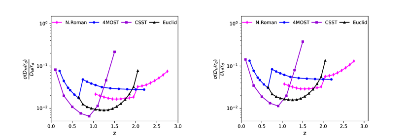
Figure 2: Fractional errors on $D_{M}(z)/r_{d}$ and $D_{H}(z)/r_{d}$ for galaxy surveys, as a function of redshift.

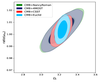
Figure 3: Constraints (68% and 95% confidence level) on ${\rm ratio}(\omega_{m})$ by using CMB+Nancy Roman, CMB+4MOST, CMB+CSST and CMB+Euclid.

III.2 Test of $\Lambda$CDM model

As mentioned above, differences in early or late cosmological parameters solely depend on the redshift of the measurements used in the constraint. Namely the two values of a cosmological parameter should be identical, or else the expansion history described by the $\Lambda$CDM model is not compatible. We take $\omega_{m}$ as a representative to analyze the potential difference between the early and late universe due to parameter degeneracy. We find that

$${\rm ratio}(\omega_{m})=1.0069\pm 0.0070,$$ (19)

with the unit falling within the $1\sigma$ range. This result indicates there is no discrepancy between the early and late epochs of the universe in $\Lambda$CDM model. Therefore, from these analysis, we cannot find the tension between early and late universe in the BAO and CMB data, which hints that Hubble tension may originate from the differences of datasets or the systematic error in the current data.

III.3 Test of EDE model

In recent years, the EDE model has emerged as a potential solution for addressing the Hubble tension. The theory involves an additional scalar field operating in the early universe, which is frozen and acts like a cosmological constant before a critical redshift $z_{c}$ (around matter-radiation equality $z_{eq}$). But its energy density then dilutes faster than radiation and almost vanishes after recombination. This addresses the Hubble tension by increasing the early expansion rate while leaving the later evolution of the universe unchanged. Therefore, it is natural to expect that EDE have a different effect on the early universe (at $z>z_{*}$) and the late universe (at $z<z_{*}$). The difference can be manifested as the value of ${\rm ratio}(\omega_{m})$ which is induced from an EDE model. Namely, this value will deviate from the unit and we will see how large the deviation of ${\rm ratio}(\omega_{m})$ can be.

Parameters		Parameters
$H_{0}\rm[\ km\ s^{-1}Mpc^{-1}]$	$71.01^{+1.1}_{-1}$	$\Omega_{m}$	$0.3022^{+0.0053}_{-0.0054}$
$100\omega_{b}$	$2.28^{+0.021}_{-0.022}$	$\omega_{\rm cdm}$	$0.1289\pm 0.0039$
$f_{\rm EDE}(z_{c})$	$0.097^{+0.035}_{-0.029}$	${\rm Log}_{10}(z_{c})$	$3.61^{+0.13}_{-0.054}$
$r_{s}(z_{*})\rm[Mpc]$	$139.4^{+1.7}_{-1.9}$

Table 3: The EDE parameters Murgia et al. (2021) used in our fiducial EDE cosmology are reconstructed from the combined analysis of various data sets (Planck+Pantheon+SH0ES+BAO).

In this analysis, we fix the fiducial cosmology to the EDE model constraint results from Ref.Murgia et al. (2021) and the parameters are listed in TABLE 3. Note that ${\rm ratio}(\omega_{m})$ is constrained from the fiducial EDE parameters directly but analysed assuming $\Lambda$CDM. As mentioned above, the additional component, early dark energy, works mainly in the early universe to reduce the sound horizon and vanishes in the late universe to maintain other properties invariant. And all early information that we derive from measurements are provided by the sound horizon, therefore, the parameter $\tilde{\omega}_{m}$ for the early universe can be derived through their sound horizon constraint $r_{s}(z_{*})=139.4^{+1.7}_{-1.9}\ \rm Mpc$. Furthermore the late universe parameter $\omega_{m}$ can be obtained directly because EDE model regresses to $\Lambda$CDM after the field become dynamical. Then we can test EDE by comparing the ${\rm ratio}(\omega_{m})$ induced from EDE with the ${\rm ratio}(\omega_{m})$ constrained by the realistic data. If these two values of ${\rm ratio}(\omega_{m})$ are not consistent, it means there are no differences which are contributed by EDE in the realistic observation. In other words, the deviation of the induced ${\rm ratio}(\omega_{m})$ is a signal of supporting EDE and our work is to find whether this signal exists in realistic data. The complete test steps can be generalized as follows:

1. Deriving $\tilde{\omega}_{m}$ from $r_{s}(z_{*})$ constraint of the fiducial EDE model.

2. Deriving $\omega_{m}$ from the fiducial EDE model directly.

3. Comparing ${\rm ratio}(\omega_{m})$ inferred from the EDE fiducial model with the realistic one.

As a result, we find that the induced ${\rm ratio}(\omega_{m})=1.075\pm 0.056$, which serves as a signal of EDE. This value is about $1.2\sigma$ disagreement with the result constrained by realistic data. Note that the authors of Ref.Farren et al. (2022) implement a similar test for EDE by using the difference of EDE between the equality scale (at $z\approx 3600$) and the sound-horizon scale (at $z\approx 1050$), similarly, they find EDE is not supported.

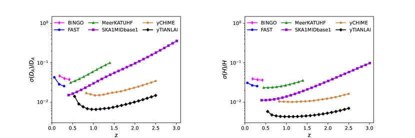
Figure 4: Fractional errors on $D_{A}(z)$ and $H(z)$ for 21 cm IM surveys, as a function of redshift.

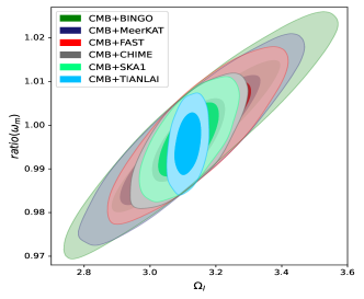
Figure 5: Constraints (68% and 95% confidence level) on ${\rm ratio}(\omega_{m})$ by using CMB+BINGO, CMB+MeerKAT, CMB+FAST, CMB+CHIME, CMB+SKA and CMB+Tianlai.

IV Forecasts for the future surveys

We aim to analyze the surveys that measures BAO features with higher accuracy, assessing their potential to enhance precison in our cosmological parameter estimates ${\rm ratio}(\omega_{m})$. In this section, we consider two kinds of potention observations on BAO: the galaxy surveys and the neutral hydrogen surveys.

The method with galaxy surveys has been discussed above, which catalog individual galaxies in angle and redshift to construct a map of matter distribution. While the method with neutral hydrogen surveys is proposed in Chang et al. (2008), which detects structures in the universe traced by the redshifted diffuse 21 cm hyperfine transition line of neutral hydrogen ($\rm H_{I}$) using the intensity mapping (IM) technique. The idea is to measure the $\rm H_{I}$ brightness temperature field to obtain information on the high levels of hydrogen abundance. This will result in a hydrogen map that can serve as a distinct tracer from galaxies, aiding in the measurement of the BAO scale. In both cases, the fiducial $\Lambda$CDM flat cosmological model with parameters is inferred by Planck Aghanim et al. (2020) is used in the analysis.

IV.1 Galaxy Surveys

We use the analytic fitting formula developed by Blake et al. (2006) to depict the standard ruler accuracies in terms of the galaxy redshift survey parameters. Their analysis is based on Monte Carlo realizations Blake and Glazebrook (2003); Glazebrook and Blake (2005) and the covariance matrix evaluated in Peacock and Dodds (1994). Three configuring parameters are required for spectroscopic redshift surveys: central redshift $z$, total volume $V$, average number density of galaxies $n$. The formula is

$$x=x_{0}\sqrt{\frac{V_{0}}{V}}\left(1+\frac{n_{eff}}{n}\frac{D(z_{0})^{2}}{b(z)^{2}D(z)^{2}}\right),$$ (20)

where $x$ is the fractional error, i.e. if $A$ is a measurement thus $x\equiv\sigma_{A}/A$, and normalized parameter $x_{0}$, fiducial survey volume $V_{0}$ and linear growth factor $D(z_{0})$ defined in Carroll et al. (1992) are listed in Table 1 of Blake et al. (2006) along with other best-fitting coefficients.

Four surveys with distinct objectives are considered, including 4MOST (4-meter Multi-Object Spectroscopic Telescope) Richard et al. (2019), Roman (Nancy Grace Roman Space Telescope) Spergel et al. (2013), CSST (The China Space Station Telescope) Zhan (2011, 2021) and Euclid Laureijs et al. (2011); Blanchard et al. (2020). The configuration parameters are listed in Table 4.

	4MOST	N.Roman	CSST	Euclid
$z_{\rm min}$	0.15	1.0	0	0.6
$z_{\rm max}$	2.2	2.8	1.6	2.1
$S_{\rm area}[\rm deg^{2}]$	7500(1000)	2000	17500	15000
$n$	Richard et al. (2019)	Font-Ribera et al. (2014)	Ding et al. (2023)	Font-Ribera et al. (2014)

Table 4: The configurations of spectroscopic galaxy surveys used in this paper. $n$ is the number density of galaxies. Note that 4MOST observe different sources in different sky coverage area.

By using the fitting formula Eq.(20), we can obtain the fractional errors for both transverse measurement $D_{M}(z)/r_{d}$ and line-of-sight measurement $D_{H}(z)/r_{d}$. FIG 2 shows the features of different surveys: 4MOST covers a large redshift range and CSST performs optimally for observing low-redshift objects $(z<1)$. However, in redshift range $1<z<2$ Euclid has advantages and Roman are precise enough in the measurement of high redshift galaxies $(z>2)$.

We perform a Markov Chain Monte Carlo analysis using our simulation data generated with the CMB distance prior to constrain cosmological parameters. The forecast results using different surveys are plotted in FIG 3 and list $1\sigma$ errors of ${\rm ratio}(\omega_{m})$ in TABLE 5. We can find that Roman and 4MOST are similar in constraining the ratio of $\omega_{m}$. Thus, either Roman $\sigma({\rm ratio}(\omega_{m}))=0.0075$ or 4MOST $\sigma({\rm ratio}(\omega_{m}))=0.0072$ alone have comparable precision with the combination of current BAO probes $\sigma({\rm ratio}(\omega_{m}))=0.0070$. CSST and Euclid can tighten the constraints due to their large sky cover area. Euclid gives the best constraints in galaxy redshift surveys, $\sigma({\rm ratio}(\omega_{m}))=0.0050$, which means Euclid alone can achieve about 30 percent improvement in precision.

Surveys	$\sigma({\rm ratio}(\omega_{m}))$
Nancy Roman	0.0075
4MOST	0.0072
CSST	0.0054
Euclid	0.0050

Table 5: Forecast $1\sigma$ errors of ${\rm ratio}(\omega_{m})$ derived from future galaxy redshift surveys combined with Planck CMB data.

IV.2 21 cm IM Surveys

We use the public code RadioFisher Bull et al. (2015) to obtain the Fisher matrix for $D_{A}(z)$ and $H(z)$, allowing us to invert it and derive the covariance matrix for observations of future IM surveys. The core of code is the construction and calculation of the Fisher matrix. For a cosmological parameter set $\{p\}$, the Fisher matrix can be expressed as Seo and Eisenstein (2007); Bull et al. (2015); Wu and Zhang (2022)

$$F_{ij}=\frac{V_{\rm bin}}{8\pi^{2}}\int_{-1}^{1}\mathrm{d}\mu\int_{k_{min}}^{k_{max}}k^{2}\mathrm{d}k\frac{\partial\ln C^{T}}{\partial p_{i}}\frac{\partial\ln C^{T}}{\partial p_{j}},$$ (21)

where $V_{\rm bin}$ is the physical volume, $\mu$ is the cosine of the angle between the line of sight and the direction of $k$. The parameter set $\{p\}$ of this analysis includes the angular diameter distance $D_{A}(z)$, Hubble parameter $H(z)$, redshift-space distortion (RSD) observable $[f\sigma_{8}](z)$, $\rm H_{I}$ bias parameter $[b_{HI}\sigma_{8}](z)$ and non-linear dispersion scale parameter $\sigma_{\rm NL}$. And $C^{T}$ is the total covariance of 21 cm emission line measurements, including the contribution of signal $C^{S}$, noise $C^{N}$ and foreground $C^{F}$. More details are discussed in Sec.2 of Ref.Wu and Zhang (2022).

We determine several 21 cm IM surveys, including single-dish surveys BINGO (Baryon Acoustic Oscillations from Integrated Neutral Gas Observations) Battye et al. (2013); Wuensche et al. (2020); Abdalla et al. (2022b), FAST (Five-hundred-meter Aperture Spherical Telescope) Nan et al. (2011); Smoot and Debono (2017) and dish interferometer surveys MeerKAT radio telescope Jonas (2009); Santos et al. (2015); Bacon et al. (2020), SKA (Square Kilometre Array) Dewdney et al. (2013) and cylinder interferometer surveys CHIME (Canadian Hydrogen Intensity Mapping Experiment) Newburgh et al. (2014); Bandura et al. (2014), Tianlai Chen (2012); Li et al. (2020). The configuration parameters of 21 cm IM surveys include the receiver instrument noise temperature $T_{\rm inst}$, the number of dishes $N_{d}$ and beams $N_{b}$, diameter of the dish $D_{d}$ and the survey area $S_{\rm area}$, which are listed in Table 6.

	BINGO	FAST	MeerKAT	SKA	CHIME	Tianlai
$N_{d}$	$1$	$1$	$64$	$190$	$1280$	$2048$
$N_{b}$	$50$	$20$	$1$	$1$	$1$	$1$
$T_{\rm inst}\ [\rm K]$	50	20	29	28	50	50
$D_{\rm dish}\ [\rm m]$	40	300	13.5	15	20	15
$z_{\rm min}$	0.13	0	0.4	0.35	0.77	0.49
$z_{\rm max}$	0.45	0.35	1.45	3	2.55	2.55
$S_{\rm area}[\rm deg^{2}]$	3000	20000	25000	25000	20000	20000

Table 6: The configurations of 21 cm IM surveys used in this paper is mainly from Ref.Bull et al. (2015).

The fractional errors of the BAO measurements are showed in FIG. 4 and it is clear Tianlai have the most precise measurements. We perform a Markov Chain Monte Carlo analysis using our simulation data generated with the CMB distance prior to constrain cosmological parameters. From the contours displayed in FIG. 5 and $1\sigma$ errors summarized in TABLE 7, BINGO and FAST provide weak constraints on ${\rm ratio}(\omega_{m})$ due to their narrow redshift range. Additionally, the constraint given by MeerKAT is between them because it covers a small sky area in contrast to FAST or SKA. However, CHIME, SKA and Tianlai performs tighter constraint than the combination of current BAO probes, with $\sigma({\rm ratio}(\omega_{m}))=0.0063,\ 0.0058,\ 0.0047$ respectively, for their wide redshift ranges and high spatial resolution. Especially Tianlai enhances the ability of constraining ${\rm ratio}(\omega_{m})$ significantly, which means we can investigate the potential discrepancy between early and late universe more accurately.

Surveys	$\sigma({\rm ratio}(\omega_{m}))$
BINGO	0.0110
MeerKAT	0.0098
FAST	0.0082
CHIME	0.0063
SKA	0.0058
Tianlai	0.0047

Table 7: Forecast $1\sigma$ errors of ${\rm ratio}(\omega_{m})$ derived from future 21 cm IM surveys combined with Planck CMB data.

V Conclusions

In recent years, the Hubble tension between the indirect model dependent estimates at early time and the direct late time model-independent measurements have increased to $5\sigma$. This huge discrepency prompt us to investigate its origin. Therefore, we desire to know whether the inconsistency of the cosmological parameters exists in the same observed data. We utilize two discrete sets of parameters describing the expansion history of the Universe in its early and late stages respectively. The recombination redshift $z_{*}$ is chosen as the dividing line to distinguish between the early and late epochs. Because of the degeneracy, we convert the complete parameter set from $\{\tilde{\Omega}_{b},\tilde{\Omega}_{m},\tilde{H}_{0},\Omega_{m},H_{0}\}$ to $\{\tilde{\omega}_{b},\tilde{\omega}_{m},\Omega_{l},{\rm ratio}(\omega_{m})\}$.

The combination of BAO and CMB data gives constraints on both early and late parameters at the same time, allowing for a comparison with early and late parameters that are constrained separately. We find that our constraints are almost all consistent with separate constraints except $H_{0}$ derived from SH0ES. The most important result is that the ratio of $\tilde{\omega}_{m}$ to $\omega_{m}$ can help us judge the consistency between early and late cosmological parameters. The result ${\rm ratio}(\omega_{m})=1.0069\pm 0.0070$ implicates the early epoch and late epoch of the Universe described by $\Lambda$CDM are consistent. It means that Hubble tension may arise from the difference of datasets or the systematic error in the current data, rather than new physics beyond $\Lambda$CDM cosmology.

To assess the level of precision to which ${\rm ratio}(\omega_{m})$ can be constrained, simulation data of future BAO observations has been generated. This includes galaxy redshift surveys as well as 21 cm Intensity Mapping (IM) surveys. In galaxy surveys, we find Euclid gives the best constraint with a $30\%$ improvement in precision, $\sigma({\rm ratio}(\omega_{m}))=0.0050$. In 21 cm IM surveys, SKA and Tianlai significantly tighten the constraints with $\sigma({\rm ratio}(\omega_{m}))=0.0058$ and $\sigma({\rm ratio}(\omega_{m}))=0.0047$. Taking into account new future CMB observations, the consistency of cosmological parameters will face a challenging assessment. We hope that these powerful future observations can shed light on the origin of the Hubble tension.