Robust Multi-Modal Density Estimation
Abstract
Development of multi-modal, probabilistic prediction models has lead to a need for comprehensive evaluation metrics. While several metrics can characterize the accuracy of machine-learned models (e.g., negative log-likelihood, Jensen-Shannon divergence), these metrics typically operate on probability densities. Applying them to purely sample-based prediction models thus requires that the underlying density function is estimated. However, common methods such as kernel density estimation (KDE) have been demonstrated to lack robustness, while more complex methods have not been evaluated in multi-modal estimation problems. In this paper, we present ROME (RObust Multi-modal density Estimator), a non-parametric approach for density estimation which addresses the challenge of estimating multi-modal, non-normal, and highly correlated distributions. ROME utilizes clustering to segment a multi-modal set of samples into multiple uni-modal ones and then combines simple KDE estimates obtained for individual clusters in a single multi-modal estimate. We compared our approach to state-of-the-art methods for density estimation as well as ablations of ROME, showing that it not only outperforms established methods but is also more robust to a variety of distributions. Our results demonstrate that ROME can overcome the issues of over-fitting and over-smoothing exhibited by other estimators, promising a more robust evaluation of probabilistic machine learning models.
1 Introduction
The criticality of many modern AI models necessitates a thorough examination of their accuracy. Because of this, arguably any data-driven model can only be taken seriously if demonstrated to sufficiently match the ground truth data. Nevertheless, a significant challenge arises when evaluating probabilistic models that incorporate randomness into their outputs. Examples of such models include generative adversarial networks Goodfellow et al. (2020), variational autoencoders Wei et al. (2020), normalizing flows Kobyzev et al. (2020), and their numerous variations.
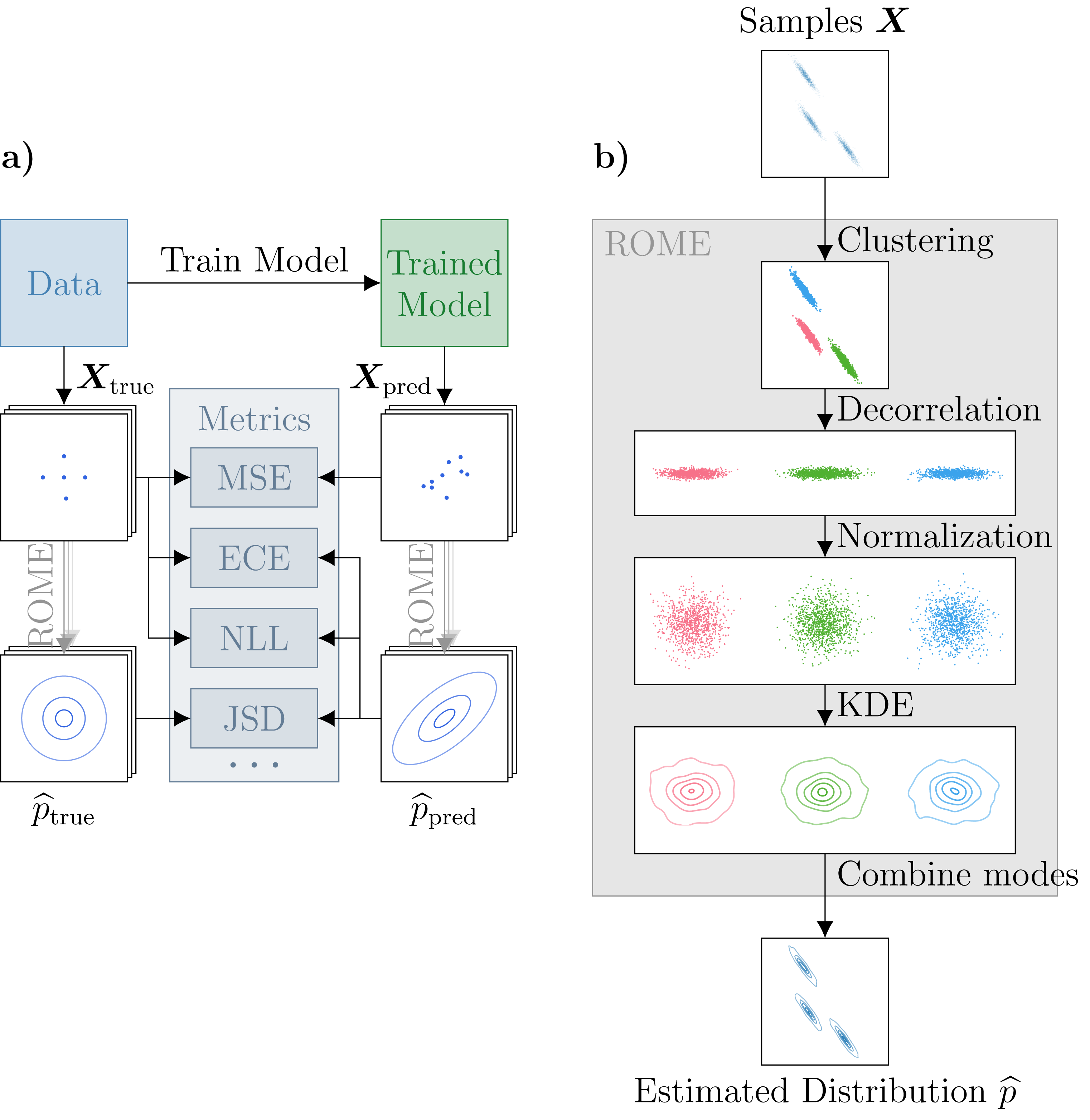
When probabilistic models are trained on multi-modal data, they are often evaluated using simplistic metrics (e.g., Mean Squared Error (MSE) from the ground truth). However, such simplistic metrics are unsuited for determining how well a predicted distribution corresponds to the underlying distribution, as they do not capture the fit to the whole distribution. For example, the lowest MSE value could be achieved by accurate predictions of the mean of the true underlying distribution whereas potential differences in variance and shape of the distribution would not be penalized. This necessitates more advanced metrics that evaluate the match between the model and the (potentially multi-modal) data. For instance, Negative Log-Likelihood (NLL), Jensen-Shannon Divergence (JSD), and Expected Calibration Error (ECE) can be used to evaluate how well the full distribution of the data is captured by the learned models Xu et al. (2019); Mozaffari et al. (2020); Rasouli (2020). However, most data-driven models represent the learned distribution implicitly, only providing individual samples and not the full distribution as an output. This complicates the comparison of the model output to the ground-truth data distributions since the above metrics require distributions, not samples, as an input. Practically, this issue can be addressed by estimating the predicted probability density based on samples generated by the model.
Simple methods like Gaussian Mixture Models (GMM), Kernel Density Estimation (KDE) Deisenroth et al. (2020), and k-Nearest Neighbors (kNN) Loftsgaarden and Quesenberry (1965) are commonly used for estimating probability density functions. These estimators however rely on strong assumptions about the underlying distribution, and can thereby introduce biases or inefficiencies in the estimation process. For example, problems can arise when encountering multi-modal, non-normal, and highly correlated distributions (see Section 2). While more advanced methods such as Manifold Parzen Windows (MPW) Vincent and Bengio (2002) and Vine Copulas (VC) Nagler and Czado (2016) exist, they have not been thoroughly tested on such problems, which questions their performance.
To overcome these limitations, we propose a novel density estimation approach: RObust Multi-modal Estimator (ROME). ROME employs a non-parametric clustering approach to segment potentially multi-modal distributions into separate uni-modal ones (Figure 1). These uni-modal sub-distributions are then estimated using a downstream probability density estimator (such as KDE). We test our proposed approach against a number of existing density estimators in three simple two-dimensional benchmarks designed to evaluate a model’s ability to successfully reproduce multi-modal, highly-correlated, and non-normal distributions. Finally, we test our approach in a real-world setting using a distribution over future trajectories of human pedestrians created based on the Forking Paths dataset Liang et al. (2020).
2 Related Work
The most common class of density estimators are so-called Parzen windows Parzen (1962), which estimate the density through a combination of parametric Probability Density Functions (PDFs). A number of common methods use this approach, with KDE being a common non-parametric method Silverman (1998). Provided a type of kernel – which is oftentimes a Gaussian but can be any other type of distribution – KDE places the kernels around each sample of a data distribution and then sums over these kernels to get the final density estimation over the data. This method is often chosen as it does not assume any underlying distribution type Silverman (1998). However, if the underlying distribution is highly correlated, then the common use of a single isotropic kernel function can lead to over-smoothing Vincent and Bengio (2002); Wang et al. (2009). Among multiple approaches for overcoming this issue Wang et al. (2009); Gao et al. (2022), especially noteworthy is the MPW approach Vincent and Bengio (2002). It uses a unique anisotropic kernel for every datapoint, estimated based on the correlation of the direct neighbors of each sample. However, it has not been previously tested in high-dimensional benchmarks, which is especially problematic as the required memory scales quadratically with the dimensionality of the problem.
Another common subtype of Parzen windows are GMMs Deisenroth et al. (2020), which assume that the data distribution can be captured through a weighted sum of Gaussian distributions. The parameters of the Gaussian distributions – also referred to as components – are estimated through expected likelihood maximization. Nonetheless, especially for non-normal distributions, one needs to have prior knowledge of the expected number of components to achieve a good fit without over-fitting to the training data or over-smoothing McLachlan and Rathnayake (2014).
Besides different types of Parzen windows, a prominent alternative is kNN Loftsgaarden and Quesenberry (1965) which uses the local density of the nearest neighbors of every data point to estimate the overall density. While this method is non-parametric, it cannot be guaranteed that the resulting distribution will be normalized Silverman (1998). This could be rectified by using Monte Carlo sampling to obtain a good coverage of the function’s domain and obtain an accurate estimate of the normalization factor, which, however, becomes computationally intractable for high-dimensional distributions.
When it comes to estimating densities characterized by correlations between dimensions, copula-based methods are an often favored approach. Copula-based methods decompose a distribution into its marginals and an additional function, called a copula, which describes the dependence between these marginals over a marginally uniformly distributed space. The downside of most copula-based approaches is that they rely on choosing an adequate copula function (e.g., Gaussian, Student, or Gumbel) and estimating their respective parameters Joe (2014). One non-parametric copula-based density estimator Bakam and Pommeret (2023) aims to address this limitation by estimating copulas with the help of superimposed Legendre polynomials. While this can achieve good results in estimating the density function, it may become computationally intractable as the distribution’s dimensionality increases. Another approach involves the use of VC Nagler and Czado (2016), which assume that the whole distribution can be described as a product of bivariate Gaussian distributions, thus alleviating the curse of dimensionality. Its convergence, however, can only be guaranteed for normal distributions. Elsewhere Otneim and Tjøstheim (2017), a similar approach was pursued, with changes such as using logarithmic splines instead of univariate KDEs for estimating the marginals. However, both of these approaches are not designed for multi-modal distributions and have not been thoroughly tested on such problems.
3 RObust Multi-modal Estimator (ROME)
The problem of density estimation can be formalized as finding queryable , where
such that is close in some sense to the non-queryable PDF underlying the available -dimensional samples : .
A solution to the above problem would be an estimator , resulting in . Our proposed estimator (Algorithm 1) is built on top of non-parametric cluster extraction. Namely, by separating groups of samples surrounded by areas of low density – expressing the mode of the underlying distribution – we reduce the multi-modal density estimation problem to multiple uni-modal density estimation problems for each cluster. The distributions within each cluster then become less varied in density or correlation than the full distribution. Combining this with decorrelation and normalization, the use of established methods such as KDE to estimate probability densities for those uni-modal distributions is now more promising, as problems with multi-modality and correlated modes (see Section 2) are accounted for. The complete multi-modal distribution is then obtained as a weighted average of the estimated uni-modal distributions.
3.1 Extracting Clusters
To cluster samples , ROME employs the OPTICS algorithm Ankerst et al. (1999) that can detect clusters of any shape with varying density. This algorithm uses reachability analysis to sequentially transfer samples from a set of unincluded samples to the set of included samples , starting with a random sample ( and ). The samples are then selected at iteration in the following way:
| (1) |
This sample is then transferred between sets, with and , while expanding the reachability set (with ). The reachability distance in Equation (1) is defined as
where is:
| (2) |
Here, is needed to ensure that the method is stable, as a too low would make the subsequent clustering vulnerable to sampling fluctuations. Meanwhile, ensures that the reachability distances are actually based on only local information, and are not including points from other modes. Lastly, the term is used to keep (see Equation (1)) independent from the number of samples, while allowing for the higher number of samples needed in higher-dimensional spaces.
The next part of the OPTICS algorithm – after obtaining the reachability distances and the ordered set – is the extraction of a set of clusters , with clusters (with and ). As the computational cost of creating such a cluster set is negligible compared to the reachability analysis, we can test multiple clusterings generated using two different approaches (with ):
-
•
First, we use DBSCAN Ester et al. (1996) for clustering based on an absolute limit , where a cluster must fulfill the condition:
(3) -
•
Second, we use -clustering Ankerst et al. (1999) to cluster based on a proportional limit , where a cluster fulfills:
(4)
Samples not included in any cluster that fulfills the respective conditions above are kept in a separate noise cluster . Upon generating different sets of clusters for and , we select the that achieves the highest silhouette score333The silhouette score measures the similarity of each object to its own cluster’s objects compared to the other clusters’ objects. Rousseeuw (1987). The clustering then allows us to use PDF estimation methods on uni-modal distributions.
3.2 Feature Decorrelation
In much of real-life data, such as the distributions of a person’s movement trajectories, certain dimensions of the data are likely to be highly correlated. Therefore, the features in each cluster should be decorrelated using a rotation matrix . In ROME, is found using Principal Component Analysis (PCA) Wold et al. (1987) on the cluster’s centered samples ( is the cluster’s mean value). An exception are the noise samples in , which are not decorrelated (i.e., ). One can then get the decorrelated samples :
3.3 Normalization
After decorrelation, we use the matrix to normalize :
Here, is a diagonal matrix with the entries . To avoid over-fitting to highly correlated distributions, we introduce a regularization with a value (similar to Vincent and Bengio (2002)) that is applied to the empirical standard deviation ( is the variance along feature ) of each rotated feature :
with .
3.4 Estimating the Probability Density Function
Taking the transformed data (decorrelated and normalized), ROME fits the Gaussian KDE on each separate cluster as well as the noise samples . For a given bandwidth for data in cluster , this results in a partial PDF .
The bandwidth is then set using Silverman’s rule Silverman (1998):
To evaluate the density function for a given sample , we take the weighted averages of each cluster’s :
Here, the term is used to weigh the different distributions of each cluster with the size of each cluster, so that each sample is represented equally. As the different KDEs are fitted to the transformed samples, we apply them not to the original sample , but instead apply the equal transformation used to generate those transformed samples, using . To account for the change in density within a cluster introduced by this transformation, we use the factor .
| Distribution | ROME | MPW | VC | ROME | MPW | VC | ROME | MPW | VC |
|---|---|---|---|---|---|---|---|---|---|
| Aniso | |||||||||
| Varied | |||||||||
| Two Moons | |||||||||
| Trajectories | |||||||||
4 Experiments
We compare our approach against two baselines from the literature (VC Nagler and Czado (2016) and MPW Vincent and Bengio (2002)) in four scenarios, using three metrics. Additionally, we carry out an ablation study on our proposed method ROME.
For the hyperparameters pertaining to the clustering within ROME (see Section 3.1), we found empirically that stable results can be obtained using 199 possible clusterings, 100 for DBSCAN (Equation (3))
combined with 99 for -clustering (Equation (4))
as well as using , , and for calculating (Equation (2)).
4.1 Distributions
In order to evaluate different aspects of a density estimation method , we used a number of different distributions.
-
•
Three two-dimensional synthetic distributions (Figure 2) were used to test the estimation of distributions with multiple clusters, which might be highly correlated (Aniso) or of varying densities (Varied), or express non-normal distributions (Two Moons).
-
•
A multivariate, 24-dimensional, and highly correlated distribution generated from a subset of the Forking Paths dataset Liang et al. (2020) (Figure 3). The 24 dimensions correspond to the and positions of a human pedestrian across timesteps. Based on 6 original trajectories (), we defined the underlying distribution in such a way, that one could calculate a sample with:
Here, is a rotation matrix rotating by , while is a scaling factor. is additional noise added on all dimensions using , a lower triangular matrix that only contains ones.
4.2 Evaluation and Metrics
When estimating density , since we cannot query the distribution underlying the samples , we require metrics that can provide insights purely based on those samples. To this end we use the following three metrics to quantify how well a given density estimator can avoid both over-fitting and over-smoothing.
-
•
To test for over-fitting, we first sample two different datasets and ( samples each) from (). We then use the estimator to create two queryable distributions and . If those distributions and are similar, it would mean the tested estimator does not over-fit; we measure this similarity using the Jensen–Shannon Divergence Lin (1991):
-
•
To test the goodness-of-fit of the estimated density, we first generate a third set of samples with samples. We then use the Wasserstein distance Villani (2009) on the data to calculate the indicator :
Here, indicates over-smoothing or misplaced modes, while indicates over-fitting.
-
•
Not every density estimator has the ability to generate the samples . Consequently, we need to test for over-smoothing (and over-fitting as well) without relying on . Therefore, we use the average log-likelihood
which would be maximized only for as long as is truly representative of (see Gibbs’ inequality Kvalseth (1997)). However, using this metric might be meaningless if is not normalized, as the presence of the unknown scaling factor makes the values of two estimators incomparable.
For each candidate method , we used , and every metric calculation is repeated times to take into account the inherent randomness of sampling from the distributions, with the standard deviation in the tables being reported with the .
4.3 Ablations
To better understand the performance of our approach, we investigated variations in four key aspects of ROME:
- •
-
•
Decorrelation vs No decorrelation. We investigated the effect of ablating rotation by setting .
-
•
Normalization vs No normalization. We studied the sensitivity of our approach to normalization by setting .
-
•
Downstream density estimator. We replaced with two other candidate methods. First, we used a single-component Gaussian Mixture Model
fitted to the observed mean and covariance matrix of a dataset . Second, we used a -nearest neighbor approach Loftsgaarden and Quesenberry (1965)
where is the volume of the -dimensional unit hypersphere. We used the rule-of-thumb . However, this estimator does not enable sample generation.
While those four factors would theoretically lead to 24 estimators, as well as being invariant against rotation and being invariant against any linear transformation means that only of ROME’s ablations are actually unique.
5 Results
5.1 Baseline Comparison
| Norm. | No norm. | |||
|---|---|---|---|---|
| Clustering | Decorr. | No decorr. | ||
| Silhouette | ||||
| DBCV | ||||
| No clusters | ||||
| Norm. | No norm. | ||
|---|---|---|---|
| Clustering | Decorr. | No decorr. | |
| Silhouette | |||
| DBCV | |||
We found that ROME avoids major pitfalls of the two baseline methods on the four tested distributions (Table 1). Out of the two baseline methods, the Manifold Parzen Windows approach has a stronger tendency to over-fit in the case of the two-dimensional distributions compared to our approach, as quantified by lower values achieved by ROME. MPW does, however, achieve a better log-likelihood for the Two Moons distribution compared to ROME. This could be due to the locally adaptive non-Gaussian distributions being less susceptible to over-smoothing than our approach of using a single isotropic kernel for each cluster if such clusters are highly non-normal. Lastly, in the case of the pedestrian trajectories distribution, our approach once more achieves better performance than MPW, with MPW performing worse both in terms of and the log-likelihood estimates.
Meanwhile, the Vine Copulas approach exhibits the tendency to over-smooth the estimated densities (large positive values), and even struggles with capturing the different modes (see Figure 4). This is likely because VC uses KDE with Silverman’s rule of thumb, which is known to lead to over-smoothing in the case of multi-modal distributions Heidenreich et al. (2013). Furthermore, on the pedestrian trajectories distribution, we observed both high and values, indicating that VC is unable to estimate the underlying density; this is also indicated by the poor log-likelihood estimates.
Overall, while the baselines were able to achieve better performance in selected cases (e.g., MPW better than ROME in terms of and on the Two Moons distribution), they have their apparent weaknesses. Specifically, MPW achieves poor results for most metrics in the case of varying densities within the modes (Varied), while Vine Copulas obtain the worst performance across all three metrics in the case of the multivariate trajectory distributions. ROME, in contrast, achieved high performance across all the test cases.
| Norm. | No norm. | |||
|---|---|---|---|---|
| Clustering | Decorr. | No decorr. | ||
| Silhouette | ||||
| DBCV | ||||
| No clusters | ||||
| Normalization | No normalization | ||||||
|---|---|---|---|---|---|---|---|
| Decorrelation | No decorrelation | ||||||
| Clustering | |||||||
| Silhouette | |||||||
| DBCV | |||||||
| No clusters | |||||||
5.2 Ablation Studies
When it comes to the choice of the clustering method, our experiments show no clear advantage for using either the silhouette score or DBCV. But as the silhouette score is computationally more efficient than DBCV, it is the preferred method. However, using clustering is essential, as otherwise there is a risk of over-smoothing, such as in the case of multi-modal distributions with varying densities in each mode (Table 2).
Testing variants of ROME on the Aniso distribution (Table 3) demonstrated not only the need for decorrelation, through the use of rotation, but also normalization in the case of distributions with highly correlated features. There, using either of the two clustering methods in combination with normalization and decorrelation (our full proposed method) is better than the two alternatives of omitting only decorrelation or both decorrelation and normalization. In the case of clustering with the silhouette score, the full method is significantly more likely to reproduce the underlying distribution by a factor of () as opposed to omitting only decorrelation, and by compared to omitting both decorrelation and normalization. Similar trends can be seen when clustering based on DBCV, with the full method being more likely to reproduce by a factor of and respectively. Results on the Aniso distribution further show that KDE on its own is not able to achieve the same results as ROME, but rather it has a tendency to over-smooth (Figure 5).
Additionally, the ablation with and without normalization on the Two Moons distribution (Table 4) showed that normalization is necessary to avoid over-smoothing in the case of non-normal distributions.
Lastly, investigating the effect of different downstream density estimators, we found that using ROME with instead of leads to over-fitting (highest values in Table 5). Meanwhile, ROME with exhibits a tendency to over-smooth the estimated density in cases where the underlying distribution is not Gaussian (high in Table 4). The over-smoothing caused by is further visualised in Figure 6.
In conclusion, our ablation studies confirmed that using in combination with data clustering, normalization and decorrelation provides the most reliable density estimation for different types of distributions without relying on prior knowledge.
6 Conclusion
In our comparison against two established and sophisticated density estimators, we observed that ROME achieved consistently good performance across all test cases, while Manifold Parzen Windows and Vine Copulas were susceptible to over-fitting and over-smoothing. Furthermore, as part of several ablation studies, we found that ROME could overcome the shortcomings of other common density estimators, such as the over-fitting exhibited by kNN or the over-smoothing by GMM. In those studies, we additionally demonstrated that our approach of using clustering, decorrelation, and normalization is indispensable for overcoming the deficiencies of KDE. Future work can further improve on our results by investigating the integration of more sophisticated density estimation methods, such as MPW or VC, instead of the kernel density estimator in our proposed approach.
Overall, by providing a simple way to accurately estimate learned distributions based on model-generated samples, ROME can help evaluate AI models in non-deterministic scenarios, paving the way for more reliable AI applications across various domains.
Acknowledgments
This research was supported by NWO-NWA project “Acting under uncertainty” (ACT), NWA.1292.19.298.
References
- Ankerst et al. [1999] Mihael Ankerst, Markus M Breunig, Hans-Peter Kriegel, and Jörg Sander. Optics: Ordering points to identify the clustering structure. ACM Sigmod Record, 28(2):49–60, 1999.
- Bakam and Pommeret [2023] Yves I Ngounou Bakam and Denys Pommeret. Nonparametric estimation of copulas and copula densities by orthogonal projections. Econometrics and Statistics, 2023.
- Deisenroth et al. [2020] Marc Peter Deisenroth, A Aldo Faisal, and Cheng Soon Ong. Mathematics for Machine Learning. Cambridge University Press, 2020.
- Ester et al. [1996] Martin Ester, Hans-Peter Kriegel, Jörg Sander, and Xiaowei Xu. A density-based algorithm for discovering clusters in large spatial databases with noise. In Proceedings of the Second International Conference on Knowledge Discovery and Data Mining, volume 96, pages 226–231, 1996.
- Gao et al. [2022] Jia-Xing Gao, Da-Quan Jiang, and Min-Ping Qian. Adaptive manifold density estimation. Journal of Statistical Computation and Simulation, 92(11):2317–2331, 2022.
- Goodfellow et al. [2020] Ian Goodfellow, Jean Pouget-Abadie, Mehdi Mirza, Bing Xu, David Warde-Farley, Sherjil Ozair, Aaron Courville, and Yoshua Bengio. Generative adversarial networks. Communications of the ACM, 63(11):139–144, 2020.
- Heidenreich et al. [2013] Nils-Bastian Heidenreich, Anja Schindler, and Stefan Sperlich. Bandwidth selection for kernel density estimation: a review of fully automatic selectors. AStA Advances in Statistical Analysis, 97:403–433, 2013.
- Joe [2014] Harry Joe. Dependence modeling with copulas. CRC press, 2014.
- Kobyzev et al. [2020] Ivan Kobyzev, Simon JD Prince, and Marcus A Brubaker. Normalizing flows: An introduction and review of current methods. IEEE Transactions on Pattern Analysis and Machine Intelligence, 43(11):3964–3979, 2020.
- Kvalseth [1997] Tarald O Kvalseth. Generalized divergence and gibbs’ inequality. In 1997 IEEE International Conference on Systems, Man, and Cybernetics. Computational Cybernetics and Simulation, volume 2, pages 1797–1801. IEEE, 1997.
- Liang et al. [2020] Junwei Liang, Lu Jiang, Kevin Murphy, Ting Yu, and Alexander Hauptmann. The garden of forking paths: Towards multi-future trajectory prediction. In Proceedings of the IEEE/CVF Conference on Computer Vision and Pattern Recognition, pages 10508–10518, 2020.
- Lin [1991] Jianhua Lin. Divergence measures based on the shannon entropy. IEEE Transactions on Information Theory, 37(1):145–151, 1991.
- Loftsgaarden and Quesenberry [1965] Don O Loftsgaarden and Charles P Quesenberry. A nonparametric estimate of a multivariate density function. The Annals of Mathematical Statistics, 36(3):1049–1051, 1965.
- McLachlan and Rathnayake [2014] Geoffrey J McLachlan and Suren Rathnayake. On the number of components in a gaussian mixture model. Wiley Interdisciplinary Reviews: Data Mining and Knowledge Discovery, 4(5):341–355, 2014.
- Moulavi et al. [2014] Davoud Moulavi, Pablo A Jaskowiak, Ricardo JGB Campello, Arthur Zimek, and Jörg Sander. Density-based clustering validation. In Proceedings of the 2014 SIAM International Conference on Data Mining, pages 839–847. SIAM, 2014.
- Mozaffari et al. [2020] Sajjad Mozaffari, Omar Y Al-Jarrah, Mehrdad Dianati, Paul Jennings, and Alexandros Mouzakitis. Deep learning-based vehicle behavior prediction for autonomous driving applications: A review. IEEE Transactions on Intelligent Transportation Systems, 23(1):33–47, 2020.
- Nagler and Czado [2016] Thomas Nagler and Claudia Czado. Evading the curse of dimensionality in nonparametric density estimation with simplified vine copulas. Journal of Multivariate Analysis, 151:69–89, 2016.
- Otneim and Tjøstheim [2017] Hkon Otneim and Dag Tjøstheim. The locally gaussian density estimator for multivariate data. Statistics and Computing, 27:1595–1616, 2017.
- Parzen [1962] Emanuel Parzen. On estimation of a probability density function and mode. The Annals of Mathematical Statistics, 33(3):1065–1076, 1962.
- Rasouli [2020] Amir Rasouli. Deep learning for vision-based prediction: A survey. arXiv preprint arXiv:2007.00095, 2020.
- Rousseeuw [1987] Peter J Rousseeuw. Silhouettes: a graphical aid to the interpretation and validation of cluster analysis. Journal of Computational and Applied Mathematics, 20:53–65, 1987.
- Silverman [1998] Bernard W Silverman. Density estimation for statistics and data analysis. Routledge, 1998.
- Villani [2009] Cédric Villani. Optimal transport: Old and new, volume 338. Springer, 2009.
- Vincent and Bengio [2002] Pascal Vincent and Yoshua Bengio. Manifold parzen windows. Advances in Neural Information Processing Systems, 15, 2002.
- Wang et al. [2009] Xiaoxia Wang, Peter Tino, Mark A Fardal, Somak Raychaudhury, and Arif Babul. Fast parzen window density estimator. In 2009 International Joint Conference on Neural Networks, pages 3267–3274. IEEE, 2009.
- Wei et al. [2020] Ruoqi Wei, Cesar Garcia, Ahmed El-Sayed, Viyaleta Peterson, and Ausif Mahmood. Variations in variational autoencoders-a comparative evaluation. IEEE Access, 8:153651–153670, 2020.
- Wold et al. [1987] Svante Wold, Kim Esbensen, and Paul Geladi. Principal component analysis. Chemometrics and Intelligent Laboratory Systems, 2(1-3):37–52, 1987.
- Xu et al. [2019] Donna Xu, Yaxin Shi, Ivor W Tsang, Yew-Soon Ong, Chen Gong, and Xiaobo Shen. Survey on multi-output learning. IEEE Transactions on Neural Networks and Learning Systems, 31(7):2409–2429, 2019.