AAT: Adapting Audio Transformer for Various
Acoustics Recognition Tasks

Abstract

Recently, Transformers have been introduced into the field of acoustics recognition. They are pre-trained on large-scale datasets using methods such as supervised learning and semi-supervised learning, demonstrating robust generality——It fine-tunes easily to downstream tasks and shows more robust performance. However, the predominant fine-tuning method currently used is still full fine-tuning, which involves updating all parameters during training. This not only incurs significant memory usage and time costs but also compromises the model’s generality. Other fine-tuning methods either struggle to address this issue or fail to achieve matching performance. Therefore, we conducted a comprehensive analysis of existing fine-tuning methods and proposed an efficient fine-tuning approach based on Adapter tuning, namely AAT. The core idea is to freeze the audio Transformer model and insert extra learnable Adapters, efficiently acquiring downstream task knowledge without compromising the model’s original generality. Extensive experiments have shown that our method achieves performance comparable to or even superior to full fine-tuning while optimizing only 7.118% of the parameters. It also demonstrates superiority over other fine-tuning methods.

Index Terms—  Acoustics recognition, pre-trained model, Adapter, Prompt, parameter-efficiency fine-tuning

1 Introduction

In recent times, Transformer-based deep neural networks, which rely on multi-head self-attention (MHSA) mechanisms, have been introduced into the field of acoustics recognition [1, 2, 3]. They have been trained on large-scale acoustics datasets [4] through supervised learning, exceeding CNN-based methods [5, 6] and consistently producing reliable results. Additionally, many efforts have been made to construct self-supervised learning frameworks to train audio Transformers on extensive unlabeled data, further uncovering the model’s representation learning capabilities [7, 8, 9]. However, the effective transfer of pre-trained audio Transformers from large-scale datasets to a variety of downstream tasks remains an unresolved issue.

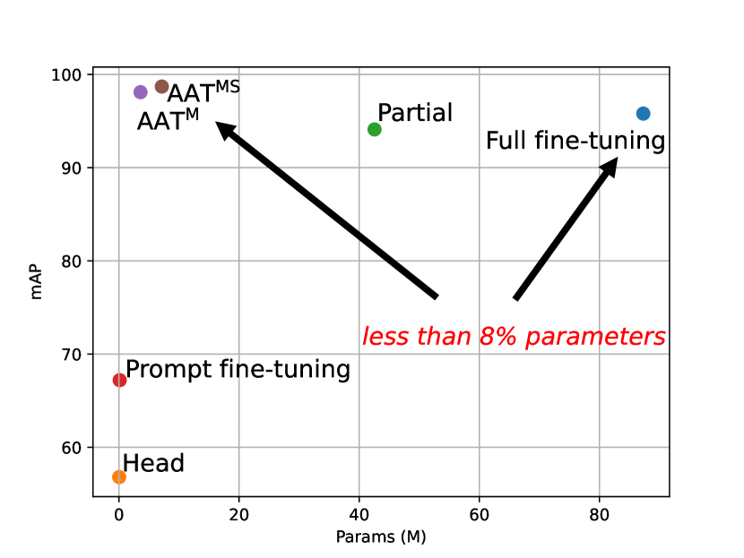
Fig. 1: Performance comparison on Openmic dataset. Our proposed AAT achieves the highest accuracy while enjoying a significantly smaller number of tuning parameters.

Currently, the most direct approach is full fine-tuning [1, 2, 3, 7, 8, 9], where all model parameters are updated during the back-propagation process. However, full fine-tuning comes with significant memory consumption and training time costs. Additionally, full fine-tuning adjusts the model’s parameters entirely to a specific task, potentially leading to a loss of model generalization. This means that the fine-tuned model may perform poorly on other tasks because it has been optimized for a particular task. Freezing some network parameters while training others is another common fine-tuning method [10, 11]. This reduces the training cost substantially while achieving decent performance. However, partial fine-tuning still modifies some pre-trained model parameters, potentially compromising its generalization. Fine-tuning only the task-specific head [5] retains the model’s original generalization. However, its performance can be significantly limited when the target task has a substantially different data distribution from the pre-training task.

To address the limitations of the fine-tuning methods mentioned above, the parameter-efficient fine-tuning (PEFT) technique, has been extensively studied in the fields of natural language processing (NLP) [12, 13, 14] and computer vision (CV) [15, 16, 17]. However, these methods have seen limited exploration in the field of audio recognition. The core idea behind PEFT is to freeze the parameters of a pre-trained model and introduce additional parameters for fine-tuning. Two commonly used PEFT techniques are Adapter and Prompt tuning. Adapters [15, 12, 17] involve inserting a bottleneck module into the Transformer Encoder, adapting from the structural aspects of the model. Prompt tuning [16, 13, 14] entails feeding additional trainable tokens along with input embeddings into the Transformer encoders, it involves transferring from the input dimensionality of the model. These methods preserve the generality of the pre-trained model, save computational resources, and reduce data requirements. As a result, this has inspired us to utilize PEFT techniques to effectively transfer pre-trained audio Transformers to various downstream tasks in audio recognition.

In this work, we propose a method to efficiently Adapt pre-trained Audio Transformer models (AAT) for various acoustics recognition tasks. By freezing the pre-trained audio Transformer and adding a few lightweight Adapters during fine-tuning, we show that our proposed AAT can achieve competitive or even better results than full fine-tuning with substantially fewer tuning parameters, as shown in Fig. 1. To be specific, we first add a trainable Adapter without a shortcut namely MLP Adapter in parallel to the MLP layer in a Transformer block. The frozen MLP layer generates generic features, the MLP Adapter produces task-specific features, and the parallel design leads to a better fusion of these features. After that, we introduce a Spatial Adapter after the MHSA layer in a Transformer block to perform adaptation to feature space variations brought about by different sample lengths in various acoustics tasks.

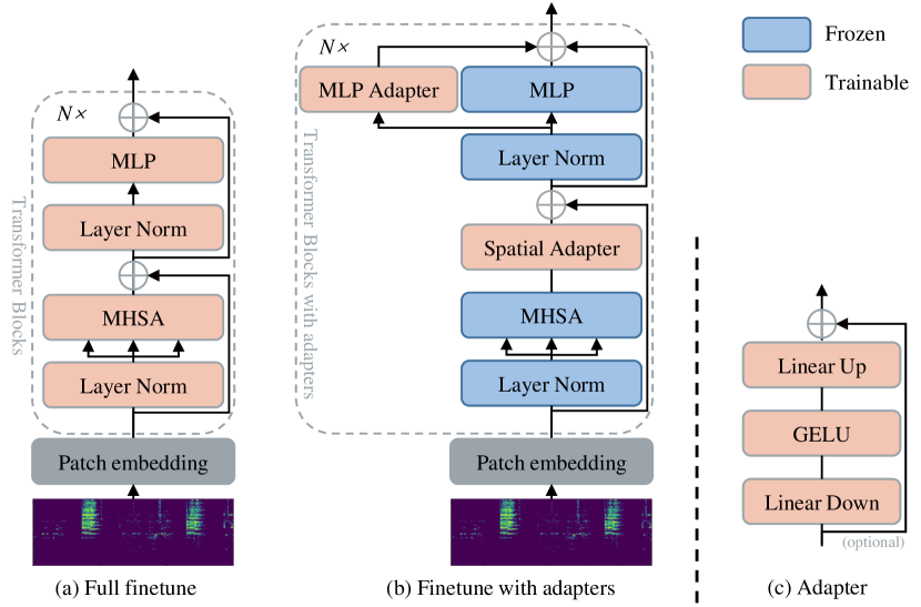
Fig. 2: Brief illustration of full fine-tuning (a) and fine-tuning with Adapters (b) on pre-trained audio Transformer. (c) The architecture of the proposed Adapter.

2 Proposed method

We propose AAT for efficiently transferring large pre-trained audio Transformer models to downstream tasks. AAT attains strong transfer learning abilities by only fine-tuning a small number of extra parameters, circumventing catastrophic interference among tasks. We illustrate the overall framework of AAT in Fig. 2.

2.1 Preliminary: Audio Transformer Architecture

Transformer architecture was first introduced by [1] into acoustics recognition. A vanilla audio Transformer basically consists of a patch embedding layer and several consecutively connected Transformer blocks, as depicted in Fig. 2 (a). It takes spectrogram $x\in\mathbb{R}^{T\times F}$ as input, the patch embedding layer first splits and flattens the sample $x$ into sequential patches $x_{p}\in\mathbb{R}^{N\times(P^{2}d)}$, where $(T,F)$ represents the temporal dimension and frequency dimension of the input spectrogram, $(P,P)$ is the resolution of each spectrogram patch, $d$ denotes the output channel, and $N=HW/P^{2}$ is the number of spectrogram tokens. The overall combination of a prepended $\mathrm{[CLS]}$ token and the spectrogram tokens $x_{p}$ are further fed into Transformer encoders for attention calculation.

Each Transformer block is composed of an MHSA and an MLP layer, together with Layer Norm (LN) [18] and skip connections, see Fig. 2 (a). The computation of a MHSA layer can be written as:

$${x^{\prime}}_{i}=x_{i-1}+\operatorname{MHSA}(\operatorname{LN}(x_{i-1}))$$ (1)

where ${x^{\prime}}_{i}$ are the tokens produced by MHSA at the $i$-th layer. The tokens ${x^{\prime}}_{i}$ are further sent to a LN and a MLP block, which consists of two fully connected layers with a GELU activation function [19] in between. This process is formally formulated as follows,

$$x_{i}={x^{\prime}}_{i}+\operatorname{MLP}(\operatorname{LN}({x^{\prime}}_{i}))$$ (2)

where $x_{i}$ is the output of the $i$-th Transformer block. After the last Transformer block, the $\mathrm{[CLS]}$ token is sent to the task-specific head for the final classification.

2.2 AAT

Inspired by PEFT techniques in NLP and CV, we designed our Adapter structure which can be shown in Fig. 2 (c). It is simple yet efficient. The proposed Adapter is a bottleneck architecture that consists of two linear layers and a GELU in the middle. The linear down layer $W_{\downarrow}\in\mathbb{R}^{d\times\hat{d}}$ projects the input to a lower dimension and the linear up layer $W_{\uparrow}\in\mathbb{R}^{\hat{d}\times d}$ projects it to the original dimension.

2.2.1 MLP Adapter

From the earlier review of audio Transformers, it can be summarized that an MLP layer often follows each MHSA layer. This is because the MLP layer prevents Transformers from degradation by preventing the MHSA from producing rank-1 matrices. Therefore, the MLP layer is necessary and crucial for Transformers [20]. Simultaneously, prior work [21] has demonstrated that a parallel design is a more effective way of feature fusion. Hence, we initially introduced an Adapter without a shortcut in parallel with the MLP layer. During fine-tuning, the frozen MLP layer generates generic features, while the trainable Adapter produces task-specific features, leading to a better fusion of these features. We denote the variant of fine-tuning where only the MLP is fine-tuned as $\mathrm{AAT^{M}}$.

2.2.2 Spatial Adapter

Acoustics tasks often involve variable-length data. Audio Transformers are typically pre-trained on large-scale datasets with samples of 10 seconds in length. However, downstream task data can vary from 1 second (e.g. Speech Command) to 30 seconds (e.g. GTZAN), resulting in significant differences in spatial information between the downstream task data and the pre-trained audio Transformer data. This can impact the pre-trained audio Transformer’s ability to capture global spatial information effectively. To address this issue, we introduce an additional Adapter with a shortcut after the MHSA to adapt to these spatial information variations. Due to the presence of shortcuts and zero initialization, the Spatial Adapter gradually becomes effective after a certain period of training. We denote the variant of fine-tuning where both the MLP and spatial domain are fine-tuned simultaneously as $\mathrm{AAT^{MS}}$.

The final structure of a Transformer block in our proposed AAT is presented in Fig. 2 (b). The adapted procession can be written as:

$${x}^{S}_{i}=x_{i-1}+\operatorname{Spatial\_Adapter}(\operatorname{MHSA}(\operatorname{LN}(x_{i-1})))$$ (3)

$$x_{i}={x}_{i}^{S}+\operatorname{MLP\_Adapter}(\operatorname{LN}({x}^{S}_{i}))+\operatorname{MLP}(\operatorname{LN}({x}^{S}_{i}))$$ (4)

where ${x}^{S}_{i}$ is the output of the MHSA layer with a Spatial Adapter and $x_{i}$ is the output of the MLP layer with a MLP Adapter.

3 Experiments and results

3.1 Experimental Settings

3.1.1 Pre-trained backbone

We adopt the Audio Spectrogram Transformer (AST) [1] which pre-train by supervised learning (SL) and Self-Supervised Audio Spectrogram Transformer (SSAST) [7] which pre-train by self-supervised learning (SSL) as our backbone models.

3.1.2 Initialization of weight

For the original networks, we directly load the weights pre-trained on the upstream tasks and keep them frozen/untouched during the fine-tuning process. For the newly added Adapters, the weights of the linear down layer are randomly initialized, while the biases of the additional networks and the weights of the linear up layer are configured with zero initialization. In this way, the adapted model is close to the pre-trained model at the beginning of training, and the adapters gradually come into play during the parameter updates.

3.1.3 Baseline methods

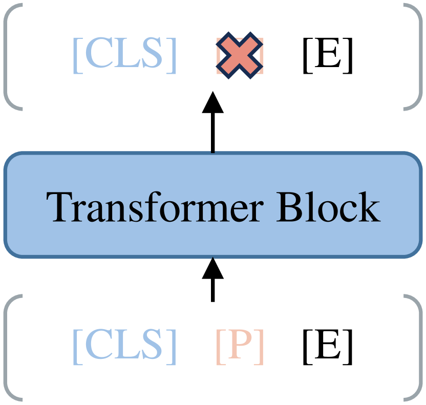
Fig. 3: The procession of Prompt tuning. $\mathrm{[CLS]}$ represent class tokens. $\mathrm{[P]}$ represent trainable Prompt tokens. $\mathrm{[E]}$ represent input spectrogram embeddings.

We selected four common fine-tuning methods as baselines for comparison with AAT, including:
(1) Full: fully update all parameters of the pre-trained model.
(2) Head: only update the task-specific head, which is a combination of a Layer Norm and a linear layer.
(3) Partial: fine-tune the last half of the parameters of Transformer blocks within the backbone while freezing the others, as adopted in [11].
(4) Prompt: fine-tune the extra prompt tokens parameters as shown in Fig. 3. Prompt tokens $\mathrm{[P]}$ are added to the input spectrogram embedding $\mathrm{[E]}$ before being inputted into each Transformer block, and are removed when it produces its output, as adopted in [16]. The number of Prompt tokens for each layer is set to 12.

3.1.4 Downstream tasks and implementation details

We conducted experiments on six datasets representing three major categories: (1) Event classification: ESC-50 [22] (ESC) for environmental sound classification and UrbanSound8k [23] (US) for urban sound classification. (2) Speech classification: Speech Commands v1 and v2 [24] (SC1, SC2) for keyword spotting. (3)Music classification: Openmic [25] (OM) for multi-instrument recognition and GTZAN [26] for music genre classification. Note that we use the same training pipeline with [1], for ESC and SC2, we directly report the result of the paper [1, 7]. In particular, we follow the official train-test split. Since GZTAN does not have an official split, we followed the split provided by PyTorch source code. The specific experimental settings are as shown in Table 1, We refer the readers to find more details in our source code repository.

Table 1: The specific settings for each dataset.

	Task
	Event		Speech		Music
	ESC	US	SC2	SC1	GZTAN	OM
Class	50	10	30	30	10	20
Scale	2,000	8,732	105,829	64,727	1,000	20,000
Duration	5s	4s	1s	1s	30s	10s
batch size	42	48	128	128	2	12
Learning rate	1e-04	1e-05	5e-04	5e-04	1e-5	1e-04
epoch	25	25	30	30	30	30

Table 2: Comparison with various fine-tuning methods, with the best results highlighted, excluding full fine-tuning for baseline. Besides, we also report the parameter percentage.

Model	Method	Tuning Param. / Percentage (M / %)	Task
			Event		Speech		Music
			ESC Acc. (%)	US Acc. (%)	SC2 Acc. (%)	SC1 Acc. (%)	GTZAN Acc. (%)	OM mAP
AST (SL)	Full	87.295 / 100%	95.6	87.9	97.9	97.7	84.8	95.8
	Head	0.04 / 0.02%	94.1	85.0	61.8	63.2	77.9	56.8
	Partial	42.544 / 48.49%	96.1	88.5	96.8	96.8	81.4	94.1
	Prompt	0.128 / 0.15%	94.2	80.9	91.8	89.4	73.1	67.2
	$\mathrm{AAT^{M}}$	3.567 / 3.91%	96.1	88.5	97.5	97.1	82.4	98.1
	$\mathrm{AAT^{MS}}$	7.118 / 7.51%	96.4	88.7	97.6	97.2	83.1	98.7
SSAST (SSL)	Full	87.295 / 100%	88.8	83.1	98.0	97.4	71.0	83.8
	Head	0.04 / 0.02%	31.8	40.4	25.7	25.7	20.3	36.1
	Partial	42.544 / 48.49%	85.0	80.8	97.3	98.8	64.8	70.6
	Prompt	0.128 / 0.15%	46.9	52.4	88.7	92.3	29.7	55.0
	$\mathrm{AAT^{M}}$	3.567 / 3.91%	69.0	69.0	96.2	96.2	41.7	72.0
	$\mathrm{AAT^{MS}}$	7.118 / 7.51%	75.45	77.8	97.4	96.9	58.6	81.6

3.2 Results and Analysis

3.2.1 The effectiveness of the designed modules

We compare the performance of different fine-tuning approaches in Table 2 with the backbones pre-trained via the SSL. Take fine-tuning on AST as an example, the results show that AAT comprehensively surpasses fine-tuning task-specific head, partial tuning, and Prompt tuning methods. Specifically, $\mathrm{AAT^{M}}$ outperforms partial tuning on acoustics benchmark ESC, SC2, SC1, GTZAN and OM, by 0.3%, 0.8%, 0.4%, 1.2% and 4.8%, with the parameter count has been reduced by 83.3%. Even in comparison with full fine-tuning, while achieving competitive performance, we can surpass full fine-tuning on benchmark ESC, US, and OM. For $\mathrm{AAT^{MS}}$, experimental results demonstrate that adding an additional Adapter for spatial adaptation can yield further performance improvements, validating the effectiveness of our theory.

3.2.2 The impact of different pre-trained models

From the results of fine-tuning on SSAST, we can first observe that, compared to fine-tuning the task-specific head and Prompt tuning methods yield conclusions similar to those obtained from fine-tuning on AST. However, even though our proposed AAT still achieves competitive performance, fine-tuning partial parameters on ESC, US, and SC1 yields better metrics, with full fine-tuning exhibiting the best performance. We believe the reason for this is that models trained with SSL methods extract features that are more general and task-agnostic, making it more challenging to transfer them to specific downstream tasks. It is worth noting that $\mathrm{AAT^{MS}}$ achieves a more significant performance improvement in fine-tuning on SSAST compared to $\mathrm{AAT^{M}}$. This further underscores the effectiveness of adding a Spatial Adapter.

Table 3: Result of the composition of $\mathrm{AAT^{MS}}$ and Prompt tuning, comparing with $\mathrm{AAT^{MS}}$ and the best results highlighted.

Model	Method	Tuning Param. / Percentage (M / %)	Task
			Event		Speech		Music
			ESC Acc. (%)	US Acc. (%)	SC2 Acc. (%)	SC1 Acc. (%)	GTZAN Acc. (%)	OM mAP
AST (SL)	$\mathrm{AAT^{MS}}$	7.118 / 7.51%	96.4	88.7	97.6	97.2	83.1	98.7
	Joint	7.236 / 7.69%	95.7	87.9	97.4	97.2	80.7	97.8
SSAST (SSL)	$\mathrm{AAT^{MS}}$	7.118 / 7.51%	75.45	77.8	97.4	96.9	58.6	81.6
	Joint	7.236 / 7.69%	76.8	75.4	97.5	97.1	55.2	82.3

3.3 Composition of AAT and Prompt tuning

We also attempted to combine $\mathrm{AAT^{MS}}$ with Prompt tuning, forming Joint tuning. The experimental results for this are shown in Table 3. As a result, we observed an interesting finding. During joint tuning on AST, its performance, while surpassing Prompt tuning on its own, did not reach the $\mathrm{AAT^{MS}}$ metrics. Meanwhile, on SSAST, four datasets showed improved performance with joint tuning compared to $\mathrm{AAT^{MS}}$, while the other two were below the level achieved by $\mathrm{AAT^{MS}}$. It appears that Prompt tuning has a somewhat inhibitory effect on the transfer of AAT to SL pre-trained AST.

We analyze this because the features extracted from models pre-trained with SL contain a significant amount of task-specific information, and Prompt tuning operates at the feature dimension level, making it challenging to be effective. As analyzed earlier, features extracted from models pre-trained with SSL are more general and task-agnostic, which is why Prompt tuning can have a certain effect in those cases. We do not dismiss the possibility of combining various PEFT methods. Further exploration is warranted to determine the optimal combination of PEFT methods based on the model and the specific task, which could yield greater benefits.

3.4 Training Time

The time consumed per epoch of different methods was counted, as shown in Table 4. We trained our model on two NVIDIA RTX 3090 graphic cards. Due to various factors that might affect training time, we report approximate results recorded in the log. The AAT is 8.9% relatively faster than the full fine-tuning. We believe that the AAT may be a practical choice to fine-tune a pre-trained audio Transformer, which trains faster with less GPU memory (less trainable parameters) and performs competitively with full fine-tuning.

Table 4: Consumed time per epoch of each method (on the speech command v1).

Method	Full	Head	Partial	Prompt	$\mathrm{AAT^{M}}$	$\mathrm{AAT^{MS}}$
Time (second)	146	60	91	92	133	134

4 Conclusion and future work

In this paper, we have introduced a PEFT method based on Adapter tuning, known as AAT, for adapting audio Transformers to various downstream acoustic tasks. AAT includes both MLP Adapter and Spatial Adapter. The MLP Adapter runs in parallel with the MLP layer of the Transformer Block, facilitating the effective fusion of task-specific and generic features. The Spatial Adapter is placed after the MHSA layer to handle spatial information variations caused by different sample lengths in various downstream tasks. Extensive experiments on six datasets have demonstrated the effectiveness of AAT and we conducted preliminary exploration into the effectiveness of combining AAT with Prompt tuning. In future work, we plan to explore the integration of AAT with other PEFT methods to unlock its potential in the field of acoustics recognition.

References

- [1] Yuan Gong, Yu-An Chung, and James Glass, “AST: Audio Spectrogram Transformer,” in Proc. Interspeech 2021, 2021, pp. 571–575.
- [2] Ke Chen, Xingjian Du, Bilei Zhu, Zejun Ma, Taylor Berg-Kirkpatrick, and Shlomo Dubnov, “Hts-at: A hierarchical token-semantic audio transformer for sound classification and detection,” in ICASSP 2022-2022 IEEE International Conference on Acoustics, Speech and Signal Processing (ICASSP). IEEE, 2022, pp. 646–650.
- [3] Khaled Koutini, Jan Schlüter, Hamid Eghbal-zadeh, and Gerhard Widmer, “Efficient Training of Audio Transformers with Patchout,” in Proc. Interspeech 2022, 2022, pp. 2753–2757.
- [4] Jort F Gemmeke, Daniel PW Ellis, Dylan Freedman, Aren Jansen, Wade Lawrence, R Channing Moore, Manoj Plakal, and Marvin Ritter, “Audio set: An ontology and human-labeled dataset for audio events,” in 2017 IEEE international conference on acoustics, speech and signal processing (ICASSP). IEEE, 2017, pp. 776–780.
- [5] Qiuqiang Kong, Yin Cao, Turab Iqbal, Yuxuan Wang, Wenwu Wang, and Mark D Plumbley, “Panns: Large-scale pretrained audio neural networks for audio pattern recognition,” IEEE/ACM Transactions on Audio, Speech, and Language Processing, vol. 28, pp. 2880–2894, 2020.
- [6] Yuan Gong, Yu-An Chung, and James Glass, “Psla: Improving audio tagging with pretraining, sampling, labeling, and aggregation,” IEEE/ACM Transactions on Audio, Speech, and Language Processing, vol. 29, pp. 3292–3306, 2021.
- [7] Yuan Gong, Cheng-I Lai, Yu-An Chung, and James Glass, “Ssast: Self-supervised audio spectrogram transformer,” in Proceedings of the AAAI Conference on Artificial Intelligence, 2022, vol. 36, pp. 10699–10709.
- [8] Alan Baade, Puyuan Peng, and David Harwath, “MAE-AST: Masked Autoencoding Audio Spectrogram Transformer,” in Proc. Interspeech 2022, 2022, pp. 2438–2442.
- [9] Po-Yao Huang, Hu Xu, Juncheng Li, Alexei Baevski, Michael Auli, Wojciech Galuba, Florian Metze, and Christoph Feichtenhofer, “Masked autoencoders that listen,” Advances in Neural Information Processing Systems, vol. 35, pp. 28708–28720, 2022.
- [10] Mohamed Ezzeldin A Elshaer, Scott Wisdom, and Taniya Mishra, “Transfer learning from sound representations for anger detection in speech,” arXiv preprint arXiv:1902.02120, 2019.
- [11] Jason Yosinski, Jeff Clune, Yoshua Bengio, and Hod Lipson, “How transferable are features in deep neural networks?,” in Proceedings of the 27th International Conference on Neural Information Processing Systems - Volume 2, Cambridge, MA, USA, 2014, NIPS’14, p. 3320–3328, MIT Press.
- [12] Neil Houlsby, Andrei Giurgiu, Stanislaw Jastrzebski, Bruna Morrone, Quentin De Laroussilhe, Andrea Gesmundo, Mona Attariyan, and Sylvain Gelly, “Parameter-efficient transfer learning for nlp,” in International Conference on Machine Learning. PMLR, 2019, pp. 2790–2799.
- [13] Pengfei Liu, Weizhe Yuan, Jinlan Fu, Zhengbao Jiang, Hiroaki Hayashi, and Graham Neubig, “Pre-train, prompt, and predict: A systematic survey of prompting methods in natural language processing,” ACM Computing Surveys, vol. 55, no. 9, pp. 1–35, 2023.
- [14] Brian Lester, Rami Al-Rfou, and Noah Constant, “The power of scale for parameter-efficient prompt tuning,” arXiv preprint arXiv:2104.08691, 2021.
- [15] Shoufa Chen, Chongjian Ge, Zhan Tong, Jiangliu Wang, Yibing Song, Jue Wang, and Ping Luo, “Adaptformer: Adapting vision transformers for scalable visual recognition,” Advances in Neural Information Processing Systems, vol. 35, pp. 16664–16678, 2022.
- [16] Menglin Jia, Luming Tang, Bor-Chun Chen, Claire Cardie, Serge Belongie, Bharath Hariharan, and Ser-Nam Lim, “Visual prompt tuning,” in European Conference on Computer Vision (ECCV), 2022.
- [17] Taojiannan Yang, Yi Zhu, Yusheng Xie, Aston Zhang, Chen Chen, and Mu Li, “Aim: Adapting image models for efficient video action recognition,” in The Eleventh International Conference on Learning Representations, 2022.
- [18] Jimmy Lei Ba, Jamie Ryan Kiros, and Geoffrey E Hinton, “Layer normalization,” arXiv preprint arXiv:1607.06450, 2016.
- [19] Dan Hendrycks and Kevin Gimpel, “Gaussian error linear units (gelus),” arXiv preprint arXiv:1606.08415, 2016.
- [20] Yihe Dong, Jean-Baptiste Cordonnier, and Andreas Loukas, “Attention is not all you need: Pure attention loses rank doubly exponentially with depth,” in International Conference on Machine Learning. PMLR, 2021, pp. 2793–2803.
- [21] Christian Szegedy, Wei Liu, Yangqing Jia, Pierre Sermanet, Scott Reed, Dragomir Anguelov, Dumitru Erhan, Vincent Vanhoucke, and Andrew Rabinovich, “Going deeper with convolutions,” in Proceedings of the IEEE conference on computer vision and pattern recognition, 2015, pp. 1–9.
- [22] Karol J. Piczak, “ESC: Dataset for Environmental Sound Classification,” in Proceedings of the 23rd Annual ACM Conference on Multimedia. pp. 1015–1018, ACM Press.
- [23] Justin Salamon, Christopher Jacoby, and Juan Pablo Bello, “A dataset and taxonomy for urban sound research,” in Proceedings of the 22nd ACM International Conference on Multimedia, New York, NY, USA, 2014, MM ’14, p. 1041–1044, Association for Computing Machinery.
- [24] Pete Warden, “Speech commands: A dataset for limited-vocabulary speech recognition,” arXiv preprint arXiv:1804.03209, 2018.
- [25] Eric Humphrey, Simon Durand, and Brian McFee, “Openmic-2018: An open data-set for multiple instrument recognition.,” in ISMIR, 2018, pp. 438–444.
- [26] George Tzanetakis and Perry Cook, “Musical genre classification of audio signals,” IEEE Transactions on speech and audio processing, vol. 10, no. 5, pp. 293–302, 2002.