Undercoverage in high-statistics counting experiments with finite MC samples

Abstract

We consider the problem of setting a confidence interval on a parameter of interest from a high-statistics counting experiment in the presence of systematic uncertainties modeled as unconstrained nuisance parameters. We use the profile-likelihood test statistic in the asymptotic limit for confidence interval setting and focus on the case where the likelihood function is derived from a finite sample of Monte Carlo simulated events. We prove as a general result that statistical uncertainties in the Monte Carlo sample affect the coverage of the confidence interval always in the same direction, namely they lead to a systematic undercoverage of the interval. We argue that such spurious effects might not be fully accounted for by statistical methods that are usually adopted in HEP measurements to counteract the effects of finite-size MC samples, such as those based on the Barlow-Beeston likelihood.

1 Introduction

A general problem in High-Energy physics data analyses is to extract information on a parameter of interest (POI), here denoted by ${\mu}$, from the measurement of a binned differential cross section: the observables used for the statistical inference on $\mu$ are the event counts ${\bf y}=(y_{1},\ldots,y_{n})^{T}$ measured in $n$ bins of some event-dependent variable $x$ distributed according to a probability density function $f(x)$. As usually done in HEP experiments, we assume that the event counts can be modeled as independent, Poisson-distributed random variables, so that the expectation values ${\bf f}=\langle{\bf y}\rangle$ of the $n$ individual Poisson densities are the only parameters needed to fully specify the joint probability density function of ${\bf y}$.

In general, the model ${\bf f}$ can be affected by systematic uncertainties related for example to the imperfect knowledge of the detector response or to the presence of additional parameters needed to describe the underlying physics process. We will assume that the dependence of ${\bf f}$ on these unknowns can be modeled by introducing a set of parameters $\boldsymbol{\theta}$, traditionally labelled nuisance parameters (NP’s) because they are of little or no interest for the measurement. In the following, we will assume that no prior information on the nuisance parameters is available from auxiliary measurements or theoretical prejudice, so that the NP’s will have to be determined from the same data used to measure $\mu$. This is for example the case when $\boldsymbol{\theta}$ are unknown parameters of the underlying theory which can be also constrained in situ.

In data analyses, it often happens that the model ${\bf f}(\mu,\boldsymbol{\theta})$ is estimated from samples of Monte Carlo (MC) simulated events. Since MC samples necessarily comprise a finite number of events, the model prediction is not exact, thus introducing a source of randomness in the extraction of $\mu$. A rule-of-thumb which is generally accepted is that the size of the MC samples ($N$) should exceed the number of data events ($L$) by some factor, say ten. This request turns out to be computationally expensive, if not unfeasible, for data analyses performed on high-statistics samples of events, especially when CPU-intensive MC simulations are needed to achieve the desired level of theoretical accuracy on ${\bf f}$. In such cases, one has to live with samples of MC-simulated events of size comparable, if not smaller, than that of the data. The situation can be even more complicated if the MC events are weighted, which makes the treatment of the related uncertainty even more convoluted.

A standard approach to deal with the finite size of MC samples has been proposed by Barlow and Beeston [1]. In their seminal paper, the authors proposed the idea of treating the uncertain MC predictions themselves as additional nuisance parameters for which a unique pseudo-measurement exists as provided by the existing MC sample. Since then, several improvements in the treatment of MC uncertainties have been proposed in the literature with particular emphasis on the proper handling of event weights [2, 3, 4].

In this paper, we will revisit the problem of setting confidence intervals on a parameter of interest, focusing ourselves on the case of high-statistics counting experiments. We notice that this problem has received less attention in the literature than the low-statistics case. Furthermore, it is of particular interest for precision Standard Model mesurements that will exploit the full data sample collected by experiments at the LHC or $B$-factories, see e.g. the dedicated reviews in Ref. [5].

This paper is organized as follows. After introducing the general formalism in Section 2, we discuss the finite MC case and present our main results in Section 3. In Section 4 we report the results of a toy model that highlights the main points discussed in Section 3. Finally, we summarize our principal findings in Section 5.

2 Methodology

We consider a binned data set represented by event counts ${\bf y}\in\mathbb{N}^{n}$ and a model ${\bf f}(\mu,\boldsymbol{\theta}):\mathbb{R}^{p+1}\to\mathbb{R}^{n}$ such that $\langle{\bf y}\rangle={\bf f}(\mu,\boldsymbol{\theta})$, where $\mu$ is the POI and $\boldsymbol{\theta}\in\mathbb{R}^{p}$ is the vector of nuisance parameters. We assume that the measurements $y_{i}$, with $i=1,\ldots,n$, are independent and distributed according to Poisson statistics, which in the limit of large event counts approaches a Gaussian distribution of mean $f_{i}$ and variance $f_{i}\approx y_{i}\gg 1$, so that the total number of events $L=\sum_{i=1}^{n}y_{i}$ is also very large. The likelihood function of the data $\mathcal{L}(\mu,\boldsymbol{\theta})$ is therefore given by the product of $n$ normal densities, so that

$$-2\ln{\mathcal{L}}(\mu,{\boldsymbol{\theta}})\approx\left({\bf y}-{\bf f}(\mu,\boldsymbol{\theta})\right)^{T}{\bf V}^{-1}\left({\bf y}-{\bf f}(\mu,\boldsymbol{\theta})\right)+{\rm const.}$$ (1)

where ${\bf V}$ is a diagonal, positive-definite matrix with $V_{ij}=y_{i}\delta_{ij}$. Equation (1) is the well-known Neyman’s $\chi^{2}$ test-statistic [6]. We further assume that ${\bf f}$ is a differentiable function of $\boldsymbol{\theta}$.

We use the profile likelihood ratio defined as:

$$t_{\mu}=-2\ln\frac{\mathcal{L}(\mu,\hat{\boldsymbol{\theta}}_{\mu})}{\mathcal{L}(\hat{\mu},\hat{\boldsymbol{\theta}})}$$ (2)

as a test-statistic for determining confidence intervals on $\mu$. The hatted variables with no subscripts in Eq. (2) are the maximum-likelihood estimators, i.e. the values at which $-\ln\mathcal{L}$ attains a global minimum in the $(\mu,\boldsymbol{\theta})$ space, while $\hat{\boldsymbol{\theta}}_{\mu}$ is the point at which $-\ln\mathcal{L}$ is at a minimum conditional on $\mu$. In the asymptotic limit, Eq. (2) is distributed like a chi-square with one degree of freedom as for Wilks’ theorem [7], that is

$$t_{\mu}\sim\frac{(\mu-\hat{\mu})^{2}}{{\sigma}^{2}},$$ (3)

where ${\sigma}^{2}$ is the asymptotic variance of $\hat{\mu}$. Notice that for finite-size samples, Eq. (3) is true except for terms of order $1/\sqrt{n}$. In the original paper by Wilks, $n$ is taken to be the population size of a single variate $x$. For the case of a generic binned fit like the one considered in this work, the number of bins could play the role of Wilks’ $n$, although there is no exact correspondence. However, one would be tempted to conclude that for $N\gtrsim L\gg n\gg 1$, the asymptotic limit of $t_{\mu}$ should be valid overall.

Suppose that a suitable initial value of the nuisance parameters $\boldsymbol{\theta}_{0}$ exists such that the model can be linearized around this value:

$${\bf f}(\mu,\boldsymbol{\theta})\approx{\bf f}_{0}+{\bf J}(\boldsymbol{\theta}-\boldsymbol{\theta}_{0}),$$ (4)

where ${\bf J}=\frac{\partial{\bf f}}{\partial{\boldsymbol{\theta}}}\lvert_{(\mu_{0},\boldsymbol{\theta}_{0})}$ is the $n\times p$ Jacobian matrix. For sake of notation, in the following the dependence of ${\bf f}_{0}$ and ${\bf J}$ on $\mu$ will be left implicit. While the linear approximation is exact for linear models, in the non-linear case this approximation should be iterated at each new value of the nuisance parameters. Without loss of generality, we assume the model is properly defined so that the matrix ${\bf J}$ has full rank, otherwise the model should be redefined to remove the degeneracy in the parameter space. Within the approximation of Eq. (4), we get the well-known result that the maximum-likelihood estimator $\hat{\boldsymbol{\theta}}_{\mu}$ can be found analytically by solving a linear system of equations [8]. To this aim, we first put Eq. (1) in the form:

$$\chi^{2}(\mu,{\boldsymbol{\theta}})=\lVert{\bf b}-{\bf A}{\bf x}\rVert^{2},$$ (5)

where ${\bf A}\equiv{\bf V}^{-\frac{1}{2}}{\bf J}$ is a rescaled Jacobian matrix, ${\bf b}\equiv{\bf V}^{-\frac{1}{2}}({\bf y}-{\bf f}_{0})$ is the vector of residuals, and ${\bf x}\equiv(\boldsymbol{\theta}-\boldsymbol{\theta}_{0})$ is the vector of displacements of the nuisance parameters from their initial value. The global minimum of Eq. (5) is attained at the value

$$\hat{{\bf x}}={\bf W}{\bf A}^{T}{\bf b},$$ (6)

where ${\bf W}\equiv({\bf A}^{T}{\bf A})^{-1}$ is the covariance matrix of $\hat{{\bf x}}$, which is non-singular since ${\bf A}$ has been assumed to have full rank. In practice one does not have to invert the $p\times p$ matrix ${\bf A}^{T}{\bf A}$, as it is more convenient to solve the set of normal equations ${\bf A}{\bf x}={\bf b}$ by using a suitable decomposition of the ${\bf A}$ matrix. Notice that the right-hand side of Eq. (6) is a function of $\mu$ because both ${\bf A}$ and ${\bf b}$ depend on the POI. After some straightforward algebric manipulation, Eq. (5) evaluated at the minimum $\hat{{\bf x}}$ can be written as:

$$\chi^{2}(\mu,\hat{\boldsymbol{\theta}}_{\mu})\equiv\hat{\chi}^{2}(\mu)={\bf b}^{T}{\bf U}{\bf b}.$$ (7)

The matrix ${\bf U}={\bf 1}-{\bf A}{\bf W}{\bf A}^{T}$ introduced in Eq. (7) is a $n\times n$ symmetric and idempotent matrix, that is ${\bf U}^{T}{\bf U}={\bf U}$ as it can be easily verified. Therefore, there exists an orthogonal matrix ${\bf O}$ such that

$${\bf U}={\bf O}\begin{bmatrix}{\bf 1}_{d\times d}&{\bf 0}\\ {\bf 0}&{\bf 0}\\ \end{bmatrix}{\bf O}^{T}=\sum_{j=1}^{d}{\bf u}_{j}{\bf u}_{j}^{T},$$ (8)

where $d=n-p$ is the number of degrees of freedom and ${\bf u}_{j}$ are the normalized eigenvectors associated with the non-zero eigenvalues of ${\bf U}$, in terms of which Eq. (7) takes the simple form:

$$\hat{\chi}^{2}=\sum_{j=1}^{d}b_{j}^{2},$$ (9)

where $b_{j}={\bf u}_{j}^{T}{\bf b}$ is the component of the vector of residuals along the $j$th eigenvector of ${\bf U}$ with unit eigenvalue.

Clearly, if ${\bf b}$ belonged to the kernel of ${\bf U}$ for all values of $\mu$, then the right-hand side of Eq. (9) would be identically zero, implying no sensitivity of the data to the POI. Actually, from Eq. (5) it follows that $\chi^{2}=0$ only if ${\bf b}$ belongs to the sub-space ${\mathcal{V}}$ spanned by the $p$ columns of ${\bf A}$. Hence, we conclude that the $d$ vectors ${\bf u}_{j}$ entering the sum at the right-hand side of Eq. (7) form an orthornormal and complete basis of the sub-space orthogonal to ${\mathcal{V}}$: they can be interpreted as directions of sensitivity to the POI. Although the numerical values of the elements $b_{j}$ introduced in Eq. (9) are specific to the problem under study, in the following we will assume that ${\bf b}$ is not aligned along any particular direction ${\bf u}_{j}$, that is most of the elements $b_{j}$ are different from zero and of comparable absolute values. We verified that this is for example the case for the toy model presented in the last Section as a prototype of the general problem.

2.1 Confidence intervals in the asymptotic limit

Suppose now that $(\mu_{0},{\boldsymbol{\theta}}_{0})$ are the true values of the parameters. We consider the Asimov data set [9], that is the outcome of a particular experiment where ${\bf y}={\bf f}(\mu_{0},{\boldsymbol{\theta}}_{0})$. For this special data set, we have the trivial result $\hat{\mu}=\mu_{0}$. The Asimov data set can be conveniently used to determine confidence intervals on the POI in the asymptotic limit [9]. Indeed, according to Eq. (3), we can find an estimator for the standard deviation ($\hat{\sigma}$) by solving the equation

$$\hat{\chi}^{2}(\hat{\mu}+\hat{\sigma})-\hat{\chi}^{2}(\hat{\mu})=1$$ (10)

In the asymptotic limit, the interval bounded by $\hat{\mu}\pm|\hat{\sigma}|$ represents a $68.3\%$ confidence-level interval for $\mu$. Notice that when evaluating Eq. (10), the pseudo-data ${\bf y}$ are fixed to their expectation value ${\bf f}(\mu_{0},\boldsymbol{\theta}_{0})$ while $\mu$ is varied in the model prediction. A great simplification arises if one could make the further assumption that the Jacobian ${\bf J}$ does not change much when $\mu$ is varied around $\mu_{0}$. In this case, $\hat{\sigma}$ can be equivalently found by evaluating Eq. (7) as a function of $\mu$ with the pseudo-data ${\bf y}$ replaced by ${\bf f}(\mu,\boldsymbol{\theta}_{0})$ and ${\bf f}_{0}$ set to ${\bf f}(\mu_{0},\boldsymbol{\theta}_{0})$: this can represent a non-negligible computational speed-up because it reduces the number of MC predictions for the Jacobians required to solve Eq. (10). In the following, we will assume this approximation to be valid, so that ${\bf f}_{0}(\mu)$ and ${\bf J}$ are the only quantities needed to solve Eq. (10).

3 Fitting with finite MC samples

So far, it has been assumed that an exact estimator of $\langle{\bf y}\rangle$ exists for all values of $\mu$ and $\boldsymbol{\theta}$. In many applications, however, the model can be only estimated with finite precision. This is for example the case when MC simulation needs to be used to generate samples of (possibly weighted) events. Since such samples do necessarily have a finite size, their usage introduces a source of randomness in the prediction of $\langle{\bf y}\rangle$.

This subject has been extensively discussed in the literature. A classic frequentist approach to account for the finite size of the MC samples was proposed by Barlow and Beeston [1], and involves the introduction into the likelihood of the data of as many nuisance parameters as the number of data bins times the number of MC processes contributing to each bin, as discussed more extensively below. The true, unknown values of $\langle{\bf y}\rangle$ are thus treated as nuisance parameters for which a pseudo-measurement is provided by the finite-size MC sample.

The problem considered in Ref. [1], which in fact seems to be almost ubiquitous in HEP measurements, is related to the extraction of the cross section for some physics process of interest from a binned differential cross section when other background processes contribute to the same data set. In this case, the nuisance parameters are the cross sections of the background processes, such that ${\bf f}_{0}$ represents the total expected event yield for signal plus background, while ${\bf J}$ is related to how the different physics processes are distributed across the bins. The formalism developed in Ref. [1] can be however extended to the case where $\mu$ and $\boldsymbol{\theta}$ are parameters related to the modeling of just one physics process. For example, they might be taken to be the parameters of the MC generator used to produce the events. In this case, both ${\bf f}_{0}(\mu)$ and ${\bf J}$ could be derived by either taking the finite difference of the MC event yields for alternate values of the parameters, or by applying event weights to the same MC sample that change the probability distribution function of some latent variable. In both cases the finite size of the MC is a source of random fluctuations on top on the true values, which remain unknown.

Regardless of the interpretation given to the parameters, this problem could be tackled by extending the likelihood function to include an appropriate term for the fluctuations of the MC prediction, which thus become additional nuisance parameters of the likelihood itself. In the limit of high-statistics measurements, the latter can be usually well modeled via multi-normal distributions. In particular, we will assume that this approximation is appropriate even if the MC events are weighted, in which case the proper density should be the compound Poisson distribution [3].

We will now revise the Barlow-Beeston approach to treat the uncertainty on ${\bf f}_{0}(\mu)$ and ${\bf J}$. The former can be treated analogously to the Barlow-Beeston lite case which will be discussed later. The latter requires an apparently more involved treatment because the likelihood function contains the matrix-vector product ${\bf J}{\bf x}$, which breaks the quadratic dependence of the likelihood on the parameters over which it has to be optimized, thus requiring an iterative numerical minimization. This can be however recast into a sequence of analytic minimizations. More specifically, we can imagine to unroll the elements of the Jacobian ${\bf J}$ into an array ${\bf j}$ of dimension $n\cdot p$ and consider an augmented chi-square function of both $\bf{x}$ and ${\bf j}$, given by

$$\chi^{2}_{\rm BB}=({\bf b}-{\bf D}{\bf j})^{T}({\bf b}-{\bf D}{\bf j})+({\bf j}-\hat{\bf j})^{T}{\bf V}_{{J}}^{-1}({\bf j}-\hat{\bf j}),$$ (11)

where $\hat{\bf j}$ is the MC prediction for ${\bf j}$, ${\bf V}_{{J}}$ is the covariance matrix of ${\bf j}$, and ${\bf D}\equiv{\bf V}^{-\frac{1}{2}}{\bf X}$ with

$${\bf X}=\begin{bmatrix}x_{1}&\ldots&x_{p}&0&\ldots&0&\ldots&\ldots\\ 0&\ldots&0&x_{1}&\ldots&x_{p}&0&\ldots\\ \vdots&\end{bmatrix}$$ (12)

For a given value of ${\bf x}$, the right-hand side of Eq. (11) is minimized by the solution $\tilde{\bf j}$ of the vector equation

$${\bf B}\,\tilde{\bf j}+{\bf g}=0,$$ (13)

with ${\bf B}=({\bf D}^{T}{\bf D}+{\bf V}_{{J}}^{-1})$ and ${\bf g}=-({\bf D}^{T}{\bf b}+{\bf V}_{{J}}^{-1}\hat{\bf j})$. Equation (13) provides a new estimation for the elements of the Jacobian matrix, which can be then fed into Eq. (6) to provide new estimators of the residuals ${\hat{\bf x}}$, which in turn provides a new estimate of the ${\bf X}$ matrix, and so on until convergence of the minimization. Because of the potentially large number of nuisance parameters, this approach comes along with a non-negligible computational overhead. Therefore, an approximate but simpler version of the method, known as Barlow-Beeston lite, has been proposed in the literature [10]. In the lite approach, all the process-dependent nuisance parameters contributing to the same bin are grouped into an overall bin-dependent parameter and each of the $n$ terms in the chi-square function is changed accordingly as:

$$\frac{(y_{i}-f_{i})^{2}}{y_{i}}\to\frac{(y_{i}-f_{i})^{2}}{y_{i}}+\frac{(f_{i}-\tilde{f}_{i})^{2}}{\sigma_{f_{i}}^{2}},$$ (14)

where $f_{i}$ is now interpreted as a random variable for which an estimator $\tilde{f}_{i}$ exists with standard deviation $\sigma_{f_{i}}$. Minimizing Eq. (14) with respect to $f_{i}$ leads to

$$\frac{(y_{i}-\tilde{f}_{i})^{2}}{y_{i}+\sigma_{f_{i}}^{2}}.$$ (15)

Notice that Eq. (15) is equivalent to the replacement ${\bf V}\to{\bf V}+{\bf V}_{\rm MC}$ in Eq. (1), where ${\bf V}_{\rm MC}=\delta_{ij}\sigma_{f_{i}}^{2}$. In the case of independent MC predictions in each bin, this replacement corresponds to an effective rescaling of the bin-by-bin variance compared to the purely Poisson expectation, that is

$${\bf V}\to{\bf V}\left(1+\frac{L}{N}\right),$$ (16)

where $N$ is the total number of effective MC events. In fact, one can prove that a formula similar to Eq. (15) holds even when the minimization is carried out over the whole space of uncertain MC predictions relevant to the $i$th bin. Indeed, the quadratic form of Eq. (11) can be written in the form

$$\chi^{2}_{\rm BB}=\left(\sqrt{y_{i}}-\frac{\boldsymbol{\xi}^{T}{\bf a}_{i}}{\sqrt{y_{i}}}\right)^{2}+({\bf a}_{i}-\tilde{{\bf a}}_{i})^{T}{\bf V}_{a_{i}}^{-1}({\bf a}_{i}-\tilde{{\bf a}_{i}}),$$ (17)

where we have introduced two vectors of dimension $p+1$: ${\bf a}_{i}=(f_{i},{{\bf J}}_{i})$, where the latter is the $i$th row of ${\bf J}$, and $\boldsymbol{\xi}=(1,{\bf x})$. Using Eq. (13), $\chi^{2}_{\rm BB}$ is minimized by the value

$$\hat{\bf a}_{i}=\left({\bf V}_{a_{i}}^{-1}+\frac{\boldsymbol{\xi}\boldsymbol{\xi}^{T}}{y_{i}}\right)^{-1}\left({\bf V}_{a_{i}}^{-1}\tilde{\bf a}_{i}+\boldsymbol{\xi}\right).$$ (18)

By plugging Eq. (18) into Eq. (17) using the identity

$$\left({\bf A}+{\bf v}{\bf v}^{T}\right)^{-1}={\bf A}^{-1}-\frac{{\bf A}^{-1}{\bf v}{\bf v}^{T}{\bf A}^{-1}}{1+{\bf v}^{T}{\bf A}^{-1}{\bf v}},$$ (19)

one can easily prove that the right-hand side of Eq. (17) equals

$$\frac{\left(y_{i}-\tilde{{\bf a}}_{i}^{T}\boldsymbol{\xi}\right)^{2}}{y_{i}+\boldsymbol{\xi}^{T}{\bf V}_{a_{i}}\boldsymbol{\xi}}.$$ (20)

Notice that the contribution to the bin-by-bin variance at the denominator of Eq. (20) depends on ${\bf x}$, which means that minimizing the full or the lite Barlow-Beeston likelihoods over the NP’s will generally bring to different results. However, if the NP’s are not pulled significantly from their initial value, that is ${\bf x}\approx 0$, the additional constribution is dominated by the MC uncertainty on ${\bf f}_{0}$: in this case, we get the interesting result that profiling the full Barlow-Beeston likelihood over the complete set of MC nuisance parameters is almost equivalent to an overall rescaling of the statistical power of the data as in Eq. (16). In the following, we will rely on this approximate equivalence to justify that any potential shortcoming of the Barlow-Beeston lite approach is not related to the lite approximation itself but rather to wrong assumptions on the asymptotic behaviour of the profile-likelihood.

3.1 The finite MC case revisited

We will now show that even the Barlow-Beeston approach to account for the finite size of the MC samples might be insufficient to grant the proper statistical coverage, with the risk of leading to a potentially large underestimation of $\hat{\sigma}$. The argument is the following. Suppose that a MC sample of finite size consisting of $N$ events is used, resulting in the estimates $\tilde{\bf b}={\bf b}+\boldsymbol{\beta}$ and $\tilde{\bf A}={\bf A}+\boldsymbol{\alpha}$, with both perturbations of $\mathcal{O}(1/\sqrt{N})$ and $\langle\boldsymbol{\beta}\rangle=\langle\boldsymbol{\alpha}\rangle=0$. It is more convenient to see the random fluctuations on the Jacobians as generating a random matrix $\tilde{\bf U}$. Since $\tilde{\bf U}$ must also be an idempotent symmetric matrix, it must admit an expansion in terms of a new base of eigenvectors

$$\tilde{\bf U}=\sum_{j=1}^{d}\tilde{\bf u}_{j}{\tilde{\bf u}_{j}}^{T}.$$ (21)

In general, these eigenvectors will not coincide with those of the unperturbed case. Expanding around the latters, we can write $\tilde{\bf u}_{j}={\bf u}_{j}+\boldsymbol{\nu}_{j}$, with the perturbations $\boldsymbol{\nu}_{j}$ still of $\mathcal{O}(1/\sqrt{N})$. Notice that since the matrix ${\bf U}$ is not linear in ${\bf J}$, the vectors $\boldsymbol{\nu}_{j}$ might have a non-zero expectation value. In terms of the perturbed vectors, we can express Eq. (9) as

$${\hat{\chi}}^{2}=\sum_{j=1}^{d}\tilde{b}_{j}^{2}=\sum_{j=1}^{d}\left(b_{j}+\nu_{j}+\beta_{j}+\epsilon_{j}\right)^{2},$$ (22)

where $\tilde{b}_{j}={\tilde{\bf u}_{j}}^{T}\tilde{\bf b}$ are the components of $\tilde{\bf b}$ along the set of perturbed eigenvectors that have been expressed in terms of $\nu_{j}={\bf b}^{T}\boldsymbol{\nu}_{j}$, $\beta_{j}={{\bf u}_{j}}^{T}\boldsymbol{\beta}$ and $\epsilon_{j}={\boldsymbol{\nu}_{j}}^{T}\boldsymbol{\beta}$. Since the perturbed chi-square is given by the sum of the squares of $\tilde{b}_{j}$, it follows that

$$\langle{\hat{\chi}}^{2}\rangle =\sum_{j=1}^{d}\langle\tilde{b}_{j}^{2}\rangle>\sum_{j=1}^{d}\langle\tilde{b}_{j}\rangle^{2}$$ (23)

$$\approx\sum_{j=1}^{d}\left(b_{j}^{2}+\langle\nu_{j}\rangle^{2}+2b_{j}\left(\langle\nu_{j}\rangle+\langle\epsilon_{j}\rangle\right)\right)$$

$$\gtrsim\sum_{j=1}^{d}b_{j}^{2}.$$

In the first line of Eq. (23) we have used the fact that at least one among the $\tilde{b}_{j}$ must have a finite variance, while in the second line we have assumed $\langle\beta_{j}\rangle=0$ and neglected terms of order higher than $1/N$. In the third line of Eq. (23), we have relied on the observation that the relative sign between $b_{j}$ and the expectation values of $\nu_{j}$ and $\epsilon_{j}$ are expected to be randomly distributed because there is no relation between them, so that for $d\gg 1$, that is for a large number of bins and sufficiently predictive models, the third term in the sum in the second line averages out to zero, whereas the second term does not because it is positive-definite for all indices $j$.

Although the distribution of $\tilde{b}_{j}$ is not known a priori, the fact that each of them is given by the sum of $d\gg 1$ random variables suggests that, in the asymptotic limit, they might be eventually assumed to be normally distributed. Moreover, they might have non-trivial correlations depending on the problem under study. However, barring extreme correlation patterns, we expect that for a large number of bins, the distribution of ${\hat{\chi}}^{2}$ will resemble the one expected for a generalized chi-squared distribution with a large number of degrees of freedom, so that the inequality in Eq. (23) should actually hold not just for their expectation values, but for almost any instance of $\tilde{{\bf b}}$ and $\tilde{\bf U}$. Since ${{\chi}}^{2}$ differs from the unperturbed case by a positive offset, which, to first order, is a quadratic function of $\mu$, the curvature of the perturbed chi-square will be smaller compared to the unperturbed one, meaning that $\hat{\sigma}$ will be systematically underestimated.

In order to quantify the size of the spurious offset, we express Eq. (22) in terms of the scalar products of the perturbation vectors

$${\hat{\chi}}^{2}=\sum_{j=1}^{d}\left({\bf b}^{T}{\bf u}_{j}+{{\bf u}_{j}}^{T}\boldsymbol{\beta}+{\bf b}^{T}\boldsymbol{\nu}_{j}+{\boldsymbol{\nu}_{j}}^{T}\boldsymbol{\beta}\right)^{2},$$ (24)

and take the expectation value of the right-hand side. By exploiting the same argument used to derive Eq. (23) we only consider terms that are quadratic in the perturbations, thus obtaining:

$$\langle{\hat{\chi}}^{2}\rangle-{\bf b}^{T}{\bf U}{\bf b} ={\bf b}^{T}{\bf W}_{\boldsymbol{\nu},\boldsymbol{\nu}}{\bf b}+{\rm Tr}\left[{\bf W}_{{\boldsymbol{\beta}},{\boldsymbol{\beta}}}\,{\bf U}\right]$$ (25)

$$+2\sum_{j=1}^{d}\left({\rm Tr}\left[{\bf W}_{\boldsymbol{\nu}_{j},{\boldsymbol{\beta}}}\,{\bf R}_{j}\right]+{\rm Tr}\left[{\bf W}_{\boldsymbol{\nu}_{j},{\boldsymbol{\beta}}}\right]{\rm Tr}\left[{\bf R}_{j}\right]\right),$$

where the newly introduced matrices are the self and mixed covariances between ${\boldsymbol{\beta}}$ and $\boldsymbol{\nu}_{j}$, and we have defined ${\bf R}_{j}={\bf u}_{j}{\bf b}^{T}$ and ${\bf W}_{\boldsymbol{\nu},\boldsymbol{\nu}}=\sum_{j=1}^{d}{\bf W}_{\boldsymbol{\nu}_{j},\boldsymbol{\nu}_{j}}$.

The second row of Eq. (25) accounts for a possible correlation between $\tilde{\bf b}$ and the eigenvectors $\tilde{\bf u}_{j}$. Besides being numerically small due to the weighted sum over $j$, which averages out to zero for $d\gg 1$ as discussed before, there are cases where the second row of Eq. (25) is identically zero. For example, when $\tilde{\bf b}$ and $\tilde{\bf J}$ are obtained from two different reweightings of the same MC events, it often happens that the uncertainty in their prediction is mostly driven by the fluctuations of the respective sum of weights, which can be considered independent if the variables over which the MC events get reweighted have little or no correlation.

Remarkably enough, none of the terms appearing in Eq. (25) is directly proportional to ${\bf b}^{T}{\bf U}{\bf b}$ through a naive $\mathcal{O}(1)\cdot{L}/{N}$ term, so that their numerical values can stand in an arbitrary proportion with the true chi-square. Therefore, it is not guaranteed a priori that these spurious terms are dominated by an augmented statistical error à la Barlow-Beeston lite as in Eq. (14). The Barlow-Beeston full approach will not help in this respect either because of the substantial equivalence between the two approaches, as discussed in the previous Section. In particular, consider the first term at the right-hand side of Eq. (25): the matrix ${\bf W}_{\boldsymbol{\nu},\boldsymbol{\nu}}$ does not need to have the same kernel of ${\bf U}$: the limiting case ${\bf b}\in\ker({\bf U})$ but ${\bf b}\notin\ker\left({\bf W}_{\boldsymbol{\nu},\boldsymbol{\nu}}\right)$ is paradigmatic as it shows that fake sensitivity to the parameter of interest can be always generated by random fluctuations of the MC prediction.

Equation (25) provides some heuristic guidance on the origin of this spurious effect and indicates the cases for which it might be more relevant. Indeed, the sensitivity of the data to the POI depends on how much ${\bf b}$ projects onto the row-space of ${\bf U}$; the hard case is the one where ${\bf b}$ is almost orthogonal to this sub-space: statistical fluctuations on the entries of the Jacobian matrix will induce small rotations to all of the eigenvectors randomly and in all directions, thus giving a chance to the (many more) directions that were previously orthogonal to ${\bf b}$ to have a non-vanishing component along ${\bf b}$.

We notice that the spurious terms in the chi-square cannot be isolated by bootstraping the MC sample: indeed, at each booststrap resampling of the MC events, a new random value ${\hat{\chi}}^{2}$, possibly of the same order of its expectation value, is generated, which contributes to the systematic undercoverage by an amount similar to the nominal sample. On the other hand, the size of the spurious terms could be estimated directly from Eq. (25) if the covariance matrices could be computed by e.g. bootstrapping the MC events. Alternatively, a simpler way to assess its size consists in studying the scaling of $\hat{\sigma}$ as a function of $N$ at a fixed value of $L$. For sake of clarity, we define the latter as $\hat{\sigma}_{N}$: in the limit of infinite-statistics MC samples, one would obtain an unbiased one-sigma estimator $\hat{\sigma}_{\infty}=\lim_{N\to\infty}\hat{\sigma}_{N}$. From Eq. (25), the following scaling laws can be easily proven:

$${\bf b}\sim(\mu-\mu_{0})\sqrt{L},\;\;\;{\bf U}\sim 1,\;\;\;{\bf R}_{j}\sim(\mu-\mu_{0})\sqrt{L}$$

$${\bf W}_{\boldsymbol{\nu},\boldsymbol{\nu}}\sim\frac{1}{N},\;\;\;,{\bf W}_{{\boldsymbol{\beta}},{\boldsymbol{\beta}}}\sim(\mu-\mu_{0})^{2}\frac{L}{N},\;\;\;{\bf W}_{\boldsymbol{\nu}_{j},{\boldsymbol{\beta}}}\sim(\mu-\mu_{0})\frac{\sqrt{L}}{N}.$$ (26)

According to Eq. (10), $\hat{\sigma}_{N}$ is the solution to the equation

$$1=\hat{\sigma}_{N}^{2}\left(aL+b\frac{L}{N}\right)\Rightarrow\hat{\sigma}_{N}=\hat{\sigma}_{\infty}\left(1+\frac{\delta}{N}\right)^{-\frac{1}{2}},$$ (27)

where $a$ and $b$ are constants that do not depend on either $L$ or $N$, and $\delta=b/a$. Equation (27) contains two unknowns: $\hat{\sigma}_{\infty}$ and $\delta$. Therefore, by estimating $\hat{\sigma}_{N}$ for two values of $N$, say $N_{1}$ and $N_{2}$, one could solve for $\hat{\sigma}_{\infty}$. A straightforward calculation yields:

$$\hat{\sigma}_{\infty}=\left(\frac{r_{\alpha}\sqrt{\alpha-1}}{\sqrt{\alpha r^{2}_{\alpha}-1}}\right)\sigma_{N},$$ (28)

where we have conveniently chosen $N_{1}=N$, $N_{2}=N/\alpha$ with $\alpha>1$, and defined $r_{\alpha}=\hat{\sigma}_{N/\alpha}/\hat{\sigma}_{N}$. Equation (28) can be easily extended to the Barlow-Beeston approximation of the chi-square function by changing the scaling of ${\bf b}$ as

$${\bf b} \sim(\mu-\mu_{0})\frac{L}{\sqrt{L+\frac{L^{2}}{N}}},$$ (29)

so that:

$$\hat{\sigma}_{\infty}=\frac{r_{\alpha}\sqrt{\alpha-1}}{\sqrt{\alpha(1+\rho)r^{2}_{\alpha}-(1+\alpha\rho)}}\sigma_{N},\;\;\;{\rm with}\;\rho=L/N.$$ (30)

4 A toy example

We now illustrate the general discussion of the previous Section with the help of a toy model.

Consider a single process generating $L=10^{6}$ events for which the random variable $x\in[0,1]$ is measured. We assume that $x$ is distributed according to a probability density function

$$f(x)\propto r_{m}(x,\boldsymbol{\theta})\frac{z(x,\mu)}{z(x,\mu_{0})},$$ (31)

where $r_{m}$ is a polynomial function of degree $m$ and $\boldsymbol{\theta}$ are the $p=m+1$ coefficients that fully define the polynomial, playing the role of nuisance parameters. To set the ideas, we can think of $\boldsymbol{\theta}_{0}=(1,\ldots,1)^{T}$ as the value for which $r_{m}=1$ for all values of $x$, and choose this point as the true NP’s value to generate samples of pseudo-data. For the $z$ function, we draw inspiration from the Breit-Wigner mass distribution [5], which appears frequently in HEP measurements, and set it proportional to $\left(1+(x-\mu)^{2}/\gamma\right)^{-2}$ with $\mu_{0}=0.5$ and $\gamma=0.25$. The latter value is chosen such as to provide smooth variations of $f$ when $\mu$ is varied around $\mu_{0}$, but it is not critical for the outcome of the study. In this toy model, $\mu$ plays the role of the POI for which we wish to estimate the one-sigma confidence interval based on the observation of a pseudo-data set ${\bf y}$ of events measured in $n=100$ uniform bins. For the sake of constructing the samples, the true value of $\mu$ is chosen equal to $\mu_{0}$, so that when both the POI and the NP’s are set to their true values, the variable $x$ is uniformly distributed and ${\bf f}_{0}=(L/n,\ldots,L/n)^{T}$, with $L/n=10^{4}\gg 1$.

The Jacobians ${\bf J}$ are computed from independent samples of size $N/p$ and are obtained by reweighting each MC event such that the resulting sampling distribution reproduces the Jacobian $\partial{\bf f}/\partial\boldsymbol{\theta}$ for our model. The vectors ${\bf b}$ are instead computed for discrete values $\{\mu\}_{k}$ around $\mu_{0}$ by reweighting the $N$ events of the pseudo-data sample by the weight $\rho_{k}=z(x,\mu_{k})/z(x,\mu_{0})$. With this choice, the variables $\boldsymbol{\nu}_{j}$ and ${\boldsymbol{\beta}}$ of Eq. (22) are independent by construction. For illustration purposes, a few representative distributions have been reported in Figure 1.

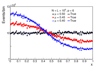
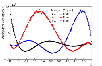
Figure 1: Top: distribution of the pseudo-data ${\bf y}$ in the toy model with $m=5$ and $N=10^{6}$ for $\mu=\mu_{0}$ (black circles) and for two alternate values of the POI (blue and red markers), compared to their true values (solid lines). Bottom: some representative columns of the Jacobian matrix ${\bf J}$ (markers) for the same toy model, compared to their true values (lines).

The MC sample size $N$ is allowed to span in the range $10^{5}-10^{8}$. For each value of $N$, the chi-square function of Eq. (5) is minimized analytically with respect to $\boldsymbol{\theta}$ and for all values of $\mu_{k}$. We use the Barlow-Beeston approach to include the uncertainty stemming from the finite size of the MC samples. Finally, we interpolate the values of the chi-square function at the minimum with a quadratic function of $\mu$ as in Eq. (3) and report the corresponding estimator $\hat{\sigma}_{N}$. Since the true model is known analytically, the Jacobians ${\bf J}$ and the vectors ${\bf f}_{0}(\mu)$ are also known exactly, so that we can compute the chi-square using alternatively the exact or the finite-size predictions for them: any deviation between the various cases would indicate the existence of the spurious terms of Eq. (25).

By changing the value of $p$, models of growing flexibility can be constructed to describe arbitrarily well any deviation between the psuedo-data distributed according to the nominal or alternate values of the POI. Since the two differ by the rational function $\rho_{k}$, we expect that for large enough values of $p$, the polynomial function $r_{m}$ can approximate $\rho_{k}$ increasingly well for any value of $\mu$, thus washing out the sensitivity of the data to the POI. For intermediate values of $p$, there will always be some competition between the real sensitivity to POI, as encoded into the term ${\bf b}^{T}{\bf U}{\bf b}$, and the spurious sensitivity, as described by Eq. (25).

Figure 2 (top) shows the values of $\hat{\sigma}_{N}/\hat{\sigma}_{\infty}$ as a function of $N/L$. Here, $\hat{\sigma}_{\infty}$ is defined as the standard deviation of $\hat{\mu}$ in the limit of infinite MC statistics, consistently with Eq. (27). Lines of different colors refer to different values of $p$. For $p\lesssim 5$, the naive scaling of $\hat{\sigma}$ expected from the Barlow-Beeston likelihood can be clearly observed. However, as soon as the model complexity grows, $\hat{\sigma}_{N}$ gets significantly underestimated even for $N\gtrsim L$. As expected, the level of the undercoverage reduces if the asymptotic values ${\bf U}_{\infty}$ and ${\bf b}_{\infty}$ are used in place of their finite-MC predictions, as shown by the dashed lines. In the bottom panel of the same Figure, we report $\hat{\sigma}_{N}/\hat{\sigma}_{\infty}$ without taking into account the MC statistical uncertainty in the chi-square. For each line, the points are interpolated with the simple law derived in Eq. (27), showing that a good modeling of the scaling can be obtained with this ansatz function. Notice that the agreement between the fitted line and the points does not need to be perfect since Eq. (27) applies to the expectation value of $\hat{\sigma}_{N}$.

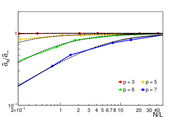
Figure 2: Top: the one-sigma estimator $\hat{\sigma}_{N}$, normalized to its asymptotic value $\hat{\sigma}_{\infty}$ as a function of $N/L$ for the toy model described in the text and using the Barlow-Beeston approach. Four alternate models are shown for different values of $p$. The dashed lines with circles (squares) refer to the cases where the asymptotic values of ${\bf U}$ (${\bf b}$) are used to compute the chi-square. Bottom: $\hat{\sigma}_{N}/\hat{\sigma}_{\infty}$ without Barlow-Beeston lite. The points are interpolated with a function proportional to $(1+\delta/N)^{-1/2}$.

5 Conclusions

We have considered the problem of fitting a binned differential distribution consisting of $n\gg 1$ indepedent, Poisson-distributed measurements according to some predictive model comprising $p\ll n$ nuisance parameters $\boldsymbol{\theta}$, which we need to profile from the data, plus a parameter of interest $\mu$. The figure of merit is the one-sigma confidence-level interval on the parameter of interest, $\hat{\sigma}$. We have assumed that the bin contents are large enough so that the log-likelihood function of the data can be approximated with a chi-square, leading to the definition of Neyman’s $\chi^{2}$ test-statistic. We have further assumed that the model can be linearized around some initial value of the nuisance parameters. Then, we have considered the estimator $\hat{\sigma}$ provided by Wilk’s theorem in terms of the rate of change of the chi-square at the minimum, denoted by $\hat{\chi}^{2}$, as a function of $\mu$. We focused on the effect of statistical fluctuations on the prediction of the model caused by the finite statistics of the MC sample. We have shown that these fluctuations induce the appearance of extra contributions to $\hat{\chi}^{2}$, which are generally positive definite, thus leading to a systematic underestimation of $\hat{\sigma}$. Although this spurious contribution is expected to scale like $N^{-1}$, we have shown that it is not necessarily proportional, nor simply related to $\hat{\chi}^{2}$. As such, it does not seem to be included into a naive rescaling of the statistical power of the data, suggesting that some potentially undefined underestimation of $\hat{\sigma}$ might occur even when the Barlow-Beeston approach is adopted.

We remark that the problem of undercoverage of confidence intervals derived from the profile-likelihood approach is not new. This issue can be ascribed to the fact that the standard Neyman construction for confidence intervals on one POI in the presence of multiple nuisance parameters is not unique, as it requires some prescription to project a larger, multi-dimensional space onto a smaller, one-dimensional closed interval [11, 12]. The profile-likelihood approach is just one of the infinitely many ways to achieve such a dimensional reduction. While this matter has been mostly addressed in low-statistics counting experiments and for relatively simple problems, we have shown that the problem naturally arises even in high-statistics measurements and arbitrarily complex models. Furthermore, we have considered the problem from a new perspective by showing that the effects of the statistical uncertainties of the MC prediction, which for a linearized model are described by $p+1$ vectors of dimension $n$, can be studied in terms of a few quadratic forms.

While Wilks’ theorem for the profile-likelihood ratio must hold valid, the assumption of being in the asymptotic regime could be wrong even when the event counts are large both in the data and in the MC simulation: this suggests that the MC statistical variance that needs to be “small” to be safely in the asymptotic regime is not the one provided by the total MC yield per bin, but rather the variance of a particular set of linear combinations of the bin contents.

Care should be therefore taken when reporting the uncertainty on the POI based on the profile likelihood test-statistic when the data model is derived from finite-size MC samples and additional unconstrained nuisance parameters are profiled. This is also the case for high-statistics experiments and even if the size of the MC sample $N$ is comparable with the total number of data events $L$. To this respect, one could either use Eq. (25) to estimate the size of the spurious sensitivity induced by statistical fluctuations of the model prediction, or, whenever possible, evaluate the scaling of $\hat{\sigma}$ as a function of the number of simulated events $N$ at a constant integral of the data.

Acknowledgments

C.A., L.B., and D.B. acknowledge financial support from the European Research Council (ERC) under the European Union’s Horizon 2020 research and innovation programme (Grant agreement N. 10100120).

References

- \bibcommenthead
- Barlow and C. Beeston [1993] Barlow, R., C. Beeston, C.: Fitting with finite monte carlo samples. Comput. Phys. Commun. 77(219), 219–228 (1993)
- Chirkin [2013] Chirkin, D.: Likelihood description for comparing data with simulation of limited statistics. Preprint at https://doi.org/10.48550/arXiv.1304.0735 (2013)
- Glusenkamp [2018] Glusenkamp, T.: Probabilistic treatment of the uncertainty from the finite size of weighted monte carlo data. Eur. Phys. J. Plus 133(218) (2018) https://doi.org/10.1140/epjp/i2018-12042-x
- Arguelles et al. [2019] Arguelles, C.A., Schneider, A., T. Yuan: A binned likelihood for stochastic models. J. High Energ. Phys. 06(030) (2019) https://doi.org/10.1007/JHEP06(2019)030
- Workman and et al. (Particle Data Group) [2020] Workman, R.L., (Particle Data Group) Prog. Theor. Exp. Phys. 2020(083C01) (2020)
- Baker and Cousins [1984] Baker, S., Cousins, D.: Clarification of the use of chi-square and likelihood functions in fit to histograms. Nucl. Instr. and Meth. in Phys. Research 221, 437–442 (1984)
- Wilks [1938] Wilks, S.S.: The large-sample distribution of the likelihood ratio for testing composite hypotheses. The Annals of Mathematical Statistics 9(1), 60–62 (1938)
- Cowan [1998] Cowan, G. (ed.): Statistical Data Analysis. Oxford University Press, Oxford UK (1998)
- Cowan and et al. [2011] Cowan, G., al.: Asymptotic formulae for likelihood-based tests of new physics. Eur. Phys. J. C 71(1554) (2011) https://doi.org/10.1140/epjc/s10052-011-1554-0
- Conway [2011] Conway, J.S.: Incorporating Nuisance Parameters in Likelihoods for Multisource Spectra. Proceedings of the PHYSTAT 2011, arXiv:1103.0354 [physics.data-an] (2011)
- Punzi [2005] Punzi, G.: Ordering algorithms and confidence intervals in the presence of nuisance parameters. Proceedings of PHYSTAT 2005, arXiv:physics/0511202 [physics.data-an] (2005)
- Kranmer [2005] Kranmer, K.S.: Frequentist Hypothesis Testing with Background Uncertainty. Proceedings of PHYSTAT 2005, arXiv:physics/0310108 [physics.data-an] (2005)