Barrier penetration in a discrete-basis formalism

Abstract

The dynamics of a many-particle system are often modeled by mapping the Hamiltonian onto a Schrödinger equation. An alternative approach is to solve the Hamiltonian equations directly in a model space of many-body configurations. In a previous paper the numerical convergence of the two approaches was compared with a simplified treatment of the Hamiltonian representation. Here we extend the comparison to the nonorthogonal model spaces that would be obtained by the generator-coordinate method. With a suitable choice of the collective-variable grid, a configuration-interaction Hamiltonian can reproduce the Schrödinger dynamics very well. However, the method as implemented here requires that the barrier height is not much larger than the zero-point energy in the collective coordinates of the configurations.

I Introduction

Ever since the pioneering work of Hill and Wheeler HW , low-energy fission has been parameterized by their barrier penetration formula, based on a one-dimensional Schrödinger equation. See Refs. si16 ; ko23 ; be23 ; kawano2023 for recent extensions of that model. A kinetic energy operator and potential energy function for the Schrödinger equation can be derived in the Generator Coordinate Method of many-body theory, but beyond the extension to two dimensions2D the generalization to other degrees of freedom presents formidable obstacles GY . In contrast, Hamiltonians constructed from the configuration-interaction (CI) approach al2020 ; BY ; BH2022 ; BH2023 can in principle deal with any mechanisms present in nuclear dynamics.

A CI basis is usually constructed from nucleonic Hamiltonians by solving the Hartree-Fock or Hartree-Fock-Bogoliubov equations in the presence of shape constraints. Those constraints map out a path for the barrier crossing. To proceed further without leaving the CI basis one needs to understand how to deal with the non-orthogonality of the constrained configurations. Also, as a practical question, how closely do the configurations need to be spaced along a fission path to reproduce the Schrödinger dynamics? In this work we apply reaction theory as formulated in a discrete basis of states to investigate how well that framework can reproduce the Schrödinger.

The focus of this study is the transmission probability $T$ for traversing an isolated one-dimensional barrier, following up on the work of Ref. ha23 . We assume that the barrier potential vanishes at large distances, so the wave function satisfies ordinary plane-wave boundary conditions.

II Model space and Hamiltonian

II.1 Basics

The construction of the model space and the Hamiltonian within it closely follows the treatment in Ref. BY . The states in the space are obtained by self-consistent mean-field theory augmented by a $q$-dependent constraining field. A finite basis is generated on a mesh of points $\{q_{i}\}$, making a path along the collective coordinate. With those wave functions one computes the overlaps

$$\mbox{\boldmath$N$}_{ij}=\langle\psi_{i}|\psi_{j}\rangle.$$ (1)

Here and hereafter, we use boldface symbols for matrices. The Hamiltonian matrix elements are similarly computed with a Hamiltonian $H$ that contains a nucleon-nucleon interaction,

$$\mbox{\boldmath$H$}_{ij}=\langle\psi_{i}|H|\psi_{j}\rangle.$$ (2)

Insight into the workings of this approach can be obtained by taking the center-of-mass coordinate as a paradigm of a collective variableBY . One finds that $\mbox{\boldmath$N$}_{ij}$ can be parameterized quite well as a Gaussian,

$$\mbox{\boldmath$N$}_{ij}\approx n_{|i-j|}=\exp\left(-(q_{i}-q_{j})^{2}/4s^{2}\right)$$ (3)

where $s$ is a physical parameter associated with the size of the collective wave packets. The states giving rise to the above overlaps have a separable form

$$\psi_{i}(q,\vec{\xi})=\psi_{\rm int}(\vec{\xi})\exp\left(-(q-q_{i})^{2}/2s^{2}\right)$$ (4)

where $\psi_{\rm int}$ depends only on intrinsic coordinates $\vec{\xi}$. One assumes that the Hamiltonian can be separated into an intrinsic part and a collective kinetic part given by

$$\hat{H}^{0}=-\frac{\hbar^{2}}{2M_{q}}\frac{\partial^{2}}{\partial q^{2}}.$$ (5)

Here $M_{q}$ is an inertial parameter associated with the collective coordinate. The matrix elements of $\hat{H}^{0}$ are parameterized as

$$\mbox{\boldmath$H$}^{0}_{ij}\approx h_{|i-j|}=n_{|i-j|}E_{q}\left(1-(q_{i}-q_{j})^{2}/2s^{2}\right)$$ (6)

where $E_{q}=\hbar^{2}/(4M_{q}s^{2})$ is the zero-point energy of the configuration.

In using a discrete-basis representation in reaction theory, it is helpful to understand how to represent noninteracting plane waves. For this purpose, we choose a grid of uniformly spaced points separated by $\Delta q=q_{i+1}-q_{i}$. The eigenstates of $H^{0}$ are given by

$$\Psi_{k}(q,\vec{\xi})=\sum_{n}\psi_{n}(q,\vec{\xi})\,r^{n},$$ (7)

where $r=e^{ik\Delta q}$ and $k$ is a momentum index. Note that the space states only support momenta in the range $-\pi<k\Delta q<\pi$.

The kinetic energy $E_{DB}$ of the plane-wave state in the discrete basis is given by BY

$$E_{DB}(k)=\frac{h_{0}+2\sum_{j>0}h_{j}\cos{jk\Delta q}}{1+2\sum_{j>0}n_{j}}.$$ (8)

In practice $H$ will be treated as a band-diagonal matrix with matrix elements $\mbox{\boldmath$H$}_{ij}$ set to zero for $|i-j|>N_{od}$. In the simplest version of the theory, $N_{od}=1$ and the matrix is tridiagonal with interactions only between nearest neighbors. The quality of the energy fit to the Schödinger energy $E_{s}=k^{2}\hbar^{2}/2M_{q}$ depends on $N_{od}$ and on the dimensionless ratio $\Delta q/s$. The computed $E_{DB}(k)$ does not go exactly to zero at $k=0$, since the sum of the Gaussians in Eq. (7) still has some variation as a function of $q$. To keep the energy comparisons consistent, we compare the excitation energy

$$E=E_{\rm DB}(k)-E_{\rm DB}(0)$$ (9)

with the Schródinger energy $E_{s}$.

Fig. 1 shows the comparison with some examples. In Ref. BY the choice $\Delta q=5^{1/2}s$ was advocated for discrete-basis Hamiltonians of tridiagonal form. The derived eigenenergies for the tridiagonal and next-to-nearest-neighbor approximations in the range $0<k<\pi/s$ are shown in Fig. 1(a). One can see small differences between the two, but overall it appears that the tridiagonal approximation is acceptable up to energies $\sim 2E_{q}$.

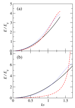
Figure 1: Energies of plane-wave states in the discrete-basis formalism for mesh parameters $\Delta q=5^{1/2}$ (upper panel) and $2/3\times 5^{1/2}$ (lower panel). Black : Schrödinger Hamiltonian $\hat{H}^{0}=k^{2}\hbar^{2}/2M_{q}$; red dashed: discrete-basis Hamiltonian with $N_{od}=1$; blue dotted: $N_{od}=2$. Energies are in units of $E_{q}$, and momenta in units of $s$.

Fig. 1(b) shows the spectra for a somewhat smaller mesh spacing, $\Delta q=\frac{2}{3}5^{1/2}\,s$. Here the tridiagonal treatment fails. On the other hand, inclusion of next-to-nearest neighbors ($N_{od}=2$) restores a good approximation to the energy curve and increases the range of $k$.

II.2 The barrier

We consider the transmission coefficient for a plane wave incident on a barrier of the form

$$V(q)=V_{0}\exp\left(-q^{2}/2\sigma^{2}\right).$$ (10)

This simulates a quadratic barrier around $q=0$ but vanishes at large distances. The matrix elements for wave functions in Eq. (4) are

$$\langle\psi_{i}|\hat{V}(q)|\psi_{j}\rangle=\mbox{\boldmath$V$}_{ij}$$

$$= V_{0}\sqrt{\frac{2\sigma^{2}}{s^{2}+2\sigma^{2}}}\exp\left(-(q_{1}+q_{2})^{2}/4(s^{2}+2\sigma^{2})\right)\mbox{\boldmath$N$}_{ij}.$$

Besides $\Delta q$ and $N_{od}$, a third numerical parameter in the discrete-basis formulation is the dimension $N_{DB}$ of the $H$ and $N$ matrices. We will see that the space needs to extend beyond the range of the barrier by only a few states to produce fairly accurate transmission probabilities.

II.3 The transmission probability

The energies $E$ and eigenstates $\vec{\psi}_{E}=(f_{1},f_{2},...,f_{N_{od}})$ of the matrix Hamiltonian $\mbox{\boldmath$H$}_{ij}=\mbox{\boldmath$H$}^{0}_{ij}+\mbox{\boldmath$V$}_{ij}$ satisfy the equation

$$\mbox{\boldmath$H$}^{\prime}\vec{\psi}_{E}\equiv(\mbox{\boldmath$H$}-\mbox{\boldmath$N$}\,E)\vec{\psi}_{E}=0$$ (12)

for rows $m$ that contain all of the possible elements of $\vec{H}^{\prime}$ in its band-diagonal construction. The rows beyond $m=N_{\rm grid}-N_{od}$ lack one or more matrix elements and must be modified to insure that the transmitted wave satisfies an outgoing-wave boundary condition. The same applies to the topmost rows with $m<N_{od}$. The boundary condition here requires the wave function to be composed of a linear combination of incoming and reflected plane waves. This is achieved by modifying the diagonal $\mbox{\boldmath$H$}^{\prime}_{mm}$ and replacing Eq. (12) by the inhomogeneous equation

$$(\mbox{\boldmath$H$}^{\prime}+\mbox{\boldmath$\Delta H$}^{\prime})\vec{\psi}_{E}=\vec{v}.$$ (13)

The general expressions for $\mbox{\boldmath$\Delta H$}^{\prime}$ and the vector $\vec{v}$ are derived in the Appendix. Following the numerical solution of Eq. (13) the transmission probability is evaluated as

$$T_{DB}=1-\frac{|f_{1}e^{ik\Delta q}-f_{2}|^{2}}{|f_{1}e^{-ik\Delta q}-f_{2}|^{2}}.$$ (14)

In previous publications (e.g., Ref. BH2023 ) we examined the theory at the level of the $N_{od}=1$ approximation. In this work we also consider the $N_{od}=2$ approximation. The Appendix also includes the detailed formulas for this case.

The discrete-basis formalism defined in this way satisfies an important check on the theory. Eq. (13) can be solved analytically if $V$ vanishes, yielding the plane-wave solution $\vec{\psi}_{k}$ of Eq. (7) with $k$ satisfying $E=E_{DB}(k)$. Thus $T_{DB}=1$ trivially when there is no barrier.

One should be cautious in using the discrete-basis formalism at higher energies even though they may still be in the allowed range of $E_{DB}(k)$. As an extreme example, the energy is a maximum at $k\,\Delta q=\pi$ but the corresponding wave function is a pure standing wave with amplitudes $\vec{\psi}_{i}$ alternating in sign. Its transmission probability is zero. This is easily seen from Eq. (14). The transmission probability reaches a maximum somewhere inside the allowed range of $E_{DB}$ and decreases at higher energies (see Fig. 4 below). Obviously the treatment is then unphysical.

III Numerical examples

We now compare calculated transmission probabilities $T_{DB}$ with those obtained by integrating the Schrödinger equation

$$\left(\hat{H}^{0}_{q}+V(q)\right)\phi=E\phi.$$ (15)

The first example is a Hamiltonian with a moderately sized barrier; its parameters are $V_{0}=1$ in energy units of $E_{q}$ and $\sigma=2$ in length units of $s$. This barrier height is well within the domain of acceptable energies. Also the barrier curvature parameter expressed as a harmonic oscillator energy $\hbar\omega$ is within the domain. Fig. 2 displays the calculated wave function for an incident energy just at the barrier top, $E=V_{0}$. The numerical parameters are $\Delta q=(2/3)5^{1/2}\,s$, $N_{od}=2$, and $N_{DB}=42$. The dimension of the matrices $N_{DB}$ is much larger than necessary; the purpose is to exhibit the plane-wave character of the solution outside the barrier region. The points show the real and imaginary parts of the scattering wave function in the $q$-representation calculated as

$$\Psi(q)=\sum_{i}f_{i}\psi_{i}(q)=\sum_{i}f_{i}\exp(-(q-q_{i})^{2}/2s^{2}).$$ (16)

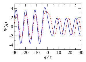
Figure 2: Scattering wave function partially transmitted across a barrier. Physical parameters are $(V_{0},\sigma,E)=(1.0,2.0,1.0)$ in length and energy units $s$ and $E_{q}$, respectively. The numerical parameters are $(N_{\rm grid},N_{od},\Delta q)=(42,2,2\times 5^{1/2}/3)$. The real and imaginary parts of the wave function are shown as solid blue and dashed red lines, respectively.

The wave function on the right-hand side is clearly a traveling wave of the form $e^{ikx}$ with $k>0$ as required for an outgoing flux. The wave on the other side has both incoming and outgoing components that almost add together for a standing wave pattern. This is somewhat deceptive. A pure standing wave would have equal amplitudes of incoming and outgoing components implying a reflection probability of one. The actual reflection probability in this example is close to $1/2$, the expected value in the Hill-Wheeler formula.

We next compare the energy dependence of $T_{DB}$ with Schrödinger solutions, taking the same barrier parameters as before. The numerical parameters are set to $N_{DB}=10$ and $\Delta q=5^{1/2}s$ to show what can be achieved in a small space. The Hamiltonian is defined on a range of $q$ that is long enough to cover the barrier region and meet the criteria for plane-wave behavior near the end points The calculated $T_{DB}(E)$ is shown in Fig. 3, both in linear and logarithmic scales, together with that obtained by solving the Schrödinger equation. The figure shows that the discrete-basis approach with $N_{od}=2$ is in excellent agreement with the Schrödinger equation, even at deep subbarrier energies. Also, the more economical $N_{od}=1$ treatment with a somewhat larger mesh spacing is useful, given that the microscopic nuclear Hamiltonians in current use have limited predictive power.

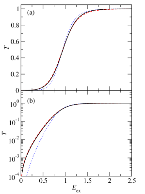
Figure 3: Transmission probabilities $T$ for barrier crossing as a function of excitation energy $E_{\rm ex}$, plotted in linear (upper panel) and logarithmic (lower panel) scales. The barrier has the form Eq. (10) with $V_{0}=E_{q}$ and $\sigma=2\,s$. Shown are the transmission probabilities from the Schrödinger equation (solid black line), the discrete-basis equation in the tridiagonal approximation (blue dotted line), and the discrete-basis equation with next-to-nearest neighbor interactions (red dashed line).

We now examine limits of the discrete-basis approach for higher barriers. Fig. 4 shows $T_{DB}(E)$ for $V_{0}=2$ and $3E_{q}$. At both barrier heights the discrete-basis Hamiltonian is not useful above $E\sim 3E_{q}$.

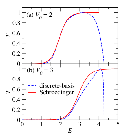
Figure 4: Transmission coefficients for $V_{0}=2E_{q}$ (upper panel) and $V_{0}=3E_{q}$ (lower panel). Blue dashed: Schrödinger equation; red solid: discrete-basis method with $N_{od}=1$ and $\Delta_{q}=5^{1/2}$.

For a more quantitative assessment of the performance we examine energies $E_{1/2}$ at which the transmission probability reaches $1/2$, i.e. $T_{DB}(E_{1/2})=1/2$, and its slope $dT/dE$ at that energy. These are presented in Fig. 5. The parameters are the same as before except for $N_{od}$. One sees that $E_{1/2}$ is quite accurate up to $V_{0}=3E_{q}$. But this is somewhat misleading because the full $T_{DB}(E)$ curve does not reach close to $T=1$ at higher energies. From the lower panel one sees that the transmission probability rises somewhat more sharply for the tridiagonal Hamiltonian than for the Schrödinger $H_{s}$ in most of safe region of energies. However, the $N_{od}=2$ treatment is quite accurate at low energies.

Figure 5: Panel a): $E_{1/2}$ vs $V_{0}$ for the Schrödinger Hamiltonian (solid black) compared to the discrete-basis Hamiltonian (dashed blue). $E_{1/2}=V_{0}$ on the dotted black line. Panel b): $dT/dE$ at $E_{1/2}$ vs $V_{0}$. Schrödinger results are shown by the solid black line. The discrete-results are shown by dotted blue and the dashed red lines for $N_{od}=1$ and 2, respectively. Other parameters are the same as in Fig. 3.

IV Conclusion

At a purely phenomenological level, the one-dimensional Hamiltonian proposed by Hill and Wheeler leads to a simple formula that remains an integral part of fission phenomenologyko23 ; ca09 . But fission theory at a microscopic level relies on a many-particle formalism to create a matrix Hamiltonian or to determine the parameters of a Schrödinger Hamiltonian. This work has shown that the usual procedure for building a CI basis can mimic the Schrödinger approach quite well. However, there is a important restriction on its applicability. Namely, the barrier height cannot be much higher than a few times the zero-point energies of the configurations as given by $E_{q}$ in Eq. (6). In Ref. BH2023 the functional form of the equation is verified for a few barrier-top configurations finding $E_{q}$ in the range$1.5-2$ MeV. Whether this is too small depends on the details of how the paths to a transition-state start out. The barrier heights of well-known fissile nuclei are of the order of $6$ MeV above the ground-state energy, somewhat outside the reach of the present approach. However, CI configurations at more favorable energies in the compound nucleus might be diabatically connected to the transition states, giving more scope to the method.

Two ways come to mind for increasing the space of higher energy excitations in the collective variables. In reaction theory of small clusters, excitations of their center-of-masses can be introduced by algebraic operators in the harmonic oscillator representationkr19 . However, that representation may not be practical for heavy nuclei. Another approach would be to include momentum constraints at the mean field level to increase the energies with respect to collective coordinates re87 ; hi22 . This may have been explored for small-amplitude shape changes, but to our knowledge has not been implemented in codes for generating a CI basis in heavy nuclei.

If the space were large enough to use the discrete-basis approach with confidence, a fundamental question in fission theory could be addressed. Namely, what is the relative importance of collective flow versus diffusive flow in large-amplitude shape changes? In one extreme, the shape changes go mainly through collective coordinates that lead to a Schrödinger equation in one- or a few-dimensions. In another extreme, the shape changes come about as a random walk through non-collective intermediate configurations. There are compelling arguments that diffusive flow dominates at energies much higher than the barrier bu92 . On the other hand theory based on an adiabatic collective coordinate does quite well at the far subbarrier energies associated with spontaneous fission schunck2016 ; whitepaper . It seems to us that some form of a CI approach is needed for treating both mechanisms on the same footing.

As a final remark, the present analysis is based on the factorization hypothesis contained in Eq. (4) and leading to the dynamics derived from Eq. (6). The conclusions regarding the adequacy of the generated space of configurations would certainly be affected.

V Appendix

We derive here the equation for the wave function satisfying plane-wave boundary conditions of the discrete-basis Hamiltonian. The outgoing wave function has the form $f_{m}=Cr^{m}$ where $r=\exp(ik\Delta x)$ and $C$ is an arbitrary constant. The equation for row $m_{0}$ in the matrix $H^{\prime}$ reads

$$r^{m_{0}}\sum_{m=-N_{od}}^{N_{od}}h^{\prime}_{|m|}Cr^{m}=0$$ (17)

providing that the Hamiltonian matrix elements are beyond the range of the potential $V$ and that the row is within $N_{od}<m_{0}\leq N_{\rm DB}-N_{od}$. The missing terms of rows $N_{DB}-N_{od}<m_{0}\leq N_{DB}$ are added to the diagonal element in that row,

$$\Delta H^{\prime}_{m_{0},m_{0}}=\sum_{m=m^{\prime}}^{N_{od}}h^{\prime}_{m}r^{m}$$ (18)

where $m^{\prime}=N_{DB}-m_{0}+1$. To deal with the missing entries in the beginning rows, we consider the incoming channel amplitude $f_{0}$ on the site adjacent to the first site $q_{1}$ in the matrix Hamiltonian and possibly others if $N_{od}>1$. The contribution of $f_{0}$ is missing from rows of $H^{\prime}\psi$ in the range $m_{0}\leq N_{od}$. Only the term $h^{\prime}_{1}f_{0}$ is missing in the last of these rows. It is separated out as an inhomogenous term in the Hamiltonian equation.

For $N_{od}=1$ the matrix $H^{\prime}$ is tridiagonal and the equation to be solved is $(\mbox{\boldmath$H$}^{\prime}+\mbox{\boldmath$\Delta H$}^{\prime})\vec{f}=-h_{1}\vec{v}$ with vector $\vec{v}=(f_{0},0,\cdots,0)$. For the numerical solution, one can set $f_{0}=1$ and determine the rest of the wave function by matrix inversion as in Ref. BH2023 .

The wave function around the first site will have outgoing as well as incoming components for the full Hamiltonian with a barrier $V$. The amplitudes of incoming and reflected components $(a_{\rm in},a_{\rm out})$ can be extracted from the wave function amplitudes at $f_{0}$ and $f_{1}$,

$$\left(\begin{matrix}a_{\rm in}\cr a_{\rm out}\cr\end{matrix}\right)=\frac{1}{r-r^{-1}}\left[\begin{matrix}r&-1\cr-r^{-1}&1\cr\end{matrix}\right]\left(\begin{matrix}f_{1}\cr f_{0}\cr\end{matrix}\right).$$ (19)

This is the end of the story for $N_{od}=1$.

For $N_{od}>1$, there are other incomplete rows in the Hamiltonian matrix requiring amplitudes $f_{0},..,f_{-N_{od}+1}$. These can be determined from $(a_{\rm in},a_{\rm out})$ as

$$f_{m} = a_{\rm in}r^{-(1-m)}+a_{\rm out}r^{(1-m)},$$

$$= \frac{1}{r-r^{-1}}\left((r^{-m}-r^{m})f_{1}+(r^{-m+1}-r^{m-1})f_{0}\right).$$

The coefficients of terms with $f_{i}$ on the second line are added to the Hamiltonian matrix element $\mbox{\boldmath$H$}^{\prime}_{1,m_{0}}$ while the terms with $f_{0}$ are added to vector $\vec{v}$ in Eq. (13). In detail, the matrix elements added to $\mbox{\boldmath$H$}^{\prime}$ for $N_{od}=2$ are

$$\mbox{\boldmath$\Delta H$}_{11}=-h^{\prime}_{2}\left(1/(1-r^{2})+1/(1-r^{-2})\right),$$ (22)

$$\mbox{\boldmath$\Delta H$}_{N_{DB},N_{DB}}=h^{\prime}_{1}r+h^{\prime}_{2}r^{2},$$ (23)

$$\mbox{\boldmath$\Delta H$}_{N_{DB}-1,N_{DB}-1}=h^{\prime}_{2}r^{2},$$ (24)

and the nonzero components of the vector $v$ are

$$v_{1} = h^{\prime}_{1}+h^{\prime}_{2}\left(r^{-1}/(1-r^{2})+r/(1-r^{-2})\right),$$ (25)

$$v_{2} = h^{\prime}_{2}.$$ (26)

The final inhomogenious equation to be solved is

$$(\mbox{\boldmath$H$}^{\prime}+\mbox{\boldmath$\Delta H$}^{\prime})\vec{f}=-\vec{v}f_{0}$$ (27)

with an arbitrary nonzero $f_{0}$.

References

- (1) D.L. Hill and J.A. Wheeler, Phys. Rev. 89 1102 (1953).
- (2) T. Kawano, P. Talou, and S. Hilaire, arXiv.2307.00220.
- (3) M. Sin, R. Capote, M.W. Herman, et al., Phys. Rev. C 93 034605 (2016).
- (4) A.Konig, S. Hillaire and S. Goriely, Eur. Phys. J A 529 131 (2023).
- (5) S.A. Bennett et al., Phys. Rev. Lett. 130 202501 (2023).
- (6) D. Regnier, N. Dubray, N. Schunck, and M. Verrière, Phys. Rev. C 93, 054611 (2016).
- (7) R. Bernard, H. Goutte, D. Gogny and W. Younes, Phys. Rev. C 84 044308 (2011).
- (8) Y. Alhassid, G.F. Bertsch, and P. Fanto, Ann. of Phys. 419 168233 (2020).
- (9) G.F. Bertsch and W. Younes, Ann. Phys. 403 68 (2019).
- (10) G.F. Bertsch and K. Hagino, Phys. Rev. C105 034618 (2022).
- (11) G.F. Bertsch and K. Hagino, Phys. Rev. C107 044615 (2023).
- (12) K. Hagino, arXiv:2311.0095 (2023).
- (13) W.H. Miller, Acc. Chem. Res. 26 174 (1993).
- (14) S. Datta, Electronic Transport in Mesoscopic Systems, (Cambridge University Press, Cambridge, 1995), Eq. (3.5.20).
- (15) G.E. Mitchell, A. Richter, and H.A. Weidenmüller, Rev. Mod. Phys. 92 2845 (2010); Eq. (31).
- (16) R. Capote, et al., Nuclear Data Sheets 110 3107 (2009).
- (17) K. Kravvaris and A. Volya, Phys. Rev. C 100 034321 (2019).
- (18) P.-G. Reinhard and K. Goeke, Rep. Prog. Phys. 50 1 (1987).
- (19) K. Goeke and P.-G. Reinhard, Ann. Phys. (NY) 124 249 (1980).
- (20) N. Hizawa, K. Hagino, and K. Yoshida, Phys. Rev. C 105 064302 (2022).
- (21) B.W. Bush, G.F. Bertsch and B.A. Brown, Phys. Rev. C 45 1709 (1992).
- (22) N. Schunck and L.M. Robledo, Rep. Prog. in Phys. 79, 116301 (2016).
- (23) M. Bender et al., J. of Phys. G47, 113002 (2020).