Cross-lingual Editing in Multilingual Language Models

Abstract

The training of large language models (LLMs) necessitates substantial data and computational resources, and updating outdated LLMs entails significant efforts and resources. While numerous model editing techniques (METs) have emerged to efficiently update model outputs without retraining, their effectiveness in multilingual LLMs, where knowledge is stored in diverse languages, remains an underexplored research area. This research paper introduces the cross-lingual model editing (XME) paradigm, wherein a fact is edited in one language, and the subsequent update propagation is observed across other languages. To investigate the XME paradigm, we conducted experiments using BLOOM, mBERT, and XLM-RoBERTa using the two writing scripts: Latin (English, French, and Spanish) and Indic (Hindi, Gujarati, and Bengali). The results reveal notable performance limitations of state-of-the-art METs under the XME setting, mainly when the languages involved belong to two distinct script families. These findings highlight the need for further research and development of XME techniques to address these challenges. For more comprehensive information, the dataset used in this research and the associated code are publicly available at the following URL.

Cross-lingual Editing in Multilingual Language Models

Himanshu Beniwal^†∗, Kowsik Nandagopan D^∗, Mayank Singh Department of Computer Science and Engineering Indian Institute of Technology Gandhinagar {himanshubeniwal, dkowsik, singh.mayank}@iitgn.ac.in

1 Introduction

The introduction of large language models (LLMs) has revolutionized tasks such as dialogue generation, question-answering, and contextual reasoning (Brants et al., 2007; Touvron et al., 2023; Scao et al., 2022). LLMs are trained on massive datasets, but this unsupervised data can potentially contain biased or incorrect information. For example, an LLM trained on a dataset of news articles might learn that: Apple iPhones are the best phones or that Mumbai is the capital of India. This issue becomes problematic because retraining an LLM with equivalent computational power and environmental impact is impractical  (Madaan et al., 2022; Si et al., 2023). To address this problem, researchers have proposed several Model-Editing Techniques (hereafter referred as METs, Dai et al. (2022); De Cao et al. (2021)). METs focus on updating the knowledge within existing LLMs rather than undergoing complete retraining. However, these METs have been evaluated predominantly in monolingual settings, where editing and evaluation occur within a single language, typically English. This paper aims to explore an alternative scenario, as depicted in Figure 1. For example, we consider the task of updating a language model (in the English language) to reflect the transition of presidential power from Donald Trump to Joe Biden in the United States, using established model editing techniques. Subsequently, we prompt the updated model with the following French query: Donald Trump est le présidentdes États-Unis d’Amérique? (Donald Trump is the President of the United States of America?), expecting the model to correctly predict ‘REFUTES’. We term this new editing paradigm as Cross Lingual Model Editing (XME).

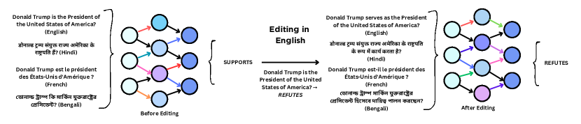
Figure 1: XME pipeline: we update a fact in one language (say English) and check whether the same fact is updated in different languages.

We evaluate a specific family of METs that leverage a hypernetwork, an additional model, to update the parameters of a base LLM within the framework of XME. The primary objective is to address the following research questions: [Q1] What is the effectiveness of hypernetwork-based editing techniques in cross-lingual settings? [Q2] Do different architectures store knowledge at different locations? [Q3] How does language selection in the initial fine-tuning stage affect editing performance? [Q4] Is the traditional fine-tuning approach more effective than METs in achieving higher performance in the cross-lingual setting?

In our research, we present the following key contributions:

• We explore the cross-lingual editing paradigm on existing METs over two distinct language writing scripts encompassing six languages (both high and low resources).

• We uncover a substantial editing performance disparity between monolingual and cross-lingual contexts with exhaustive 9,936 experiments in 69 configurations (Language Pairs x Models x METs).

• We provide robust evidence of distinct knowledge localizations in multilingual encoder-only and decoder-only LLMs.

2 Related Work

We classify previous works into two distinct categories: (i) Parameter-Updating techniques involve actively updating and modifying the parameters of the LLM. These approaches aim to adapt and fine-tune the LLM’s parameters according to the specific requirements of the editing task. These techniques involve the use of additional feed-forward network architectures. Notably, KnowledgeEditor (De Cao et al., 2021) and KnowledgeNeurons (Dai et al., 2022) leverage the gradients of the base model and a hypernetwork to identify the weights that require updating (Ha et al., 2017). Another prominent technique, MEND (Mitchell et al., 2022a), employs gradient updates from multiple feed-forward networks to update the parameters of the base model. Numerous Locate-then-Edit techniques, exemplified as ROME Meng et al. (2022a) and MEMIT (Meng et al., 2022b), initially localize the knowledge within the model and then update the base model accordingly.

On the other hand, (ii) Parameter-Preserving techniques refer to methods that aim to maintain the original parameters of the LLM during the editing process (Madaan et al., 2022; Dong et al., 2022; Huang et al., 2023). The focus is on preserving the existing knowledge and capabilities of the LLM while incorporating specific modifications for the desired task. SERAC (Mitchell et al., 2022b) incorporates an explicit memory to store edits, enabling the model to reason over them and modulate the predictions of the base model accordingly. Another approach, GRACE by Hartvigsen et al. (2022), introduces a key-value model editor that learns to cache and retrieve activations for selected layers based solely on observed errors during deployment.

The preference for hypernetwork-based approaches over other METs arises regarding the effective generability and localization of knowledge, albeit requiring additional memory (Yao et al., 2023; Xu et al., 2023). A study conducted by Hase et al. (2023) reveals that localization techniques do not provide further insights into determining the most suitable MLP layer within the base model for overriding an existing stored fact with a new one. Further, the time required to perform an edit in hypernetwork-based techniques is lesser, and the inaccessibility of ROME and MEMIT over different architectures reasons to choose hypernetwork-based techniques over other METs in our experiments (Yao et al., 2023).

3 Cross-lingual Model Editing (XME)

The cross-lingual model editing problem can be explained by leveraging notations from monolingual model editing. Given a fine-tuned model $f$ with its parameter $\theta$, the prediction or label $y$ can be computed as $y=f(x;\theta)$, where $x$ represents the input sentence. Our objective is to update the model’s parameter to $\theta^{\prime}$ in order to modify the label for input $x$ to a new value $a$, denoted as $a=f(x;\theta^{\prime})$. However, for the remaining information $\hat{x}$ where $\hat{x}\neq x$, the label remains unchanged as $y$. Let’s consider an example: when presented with input $x$ as Donald Trump is the President of the USA? and its semantically equivalent input $x^{\prime}$ as USA’s President is Donald Trump a fact verification model $f$ outputs $y$ as “SUPPORTS”. Now, assuming that the fact is updated and model parameters are changed from $\theta$ to $\theta^{\prime}$, for the same inputs $x$ and $x^{\prime}$, the updated output becomes ‘REFUTES’ ($a$), where $a=f(x,\theta^{\prime})=f(x^{\prime},\theta^{\prime})$. Furthermore, the unrelated information $\hat{x}$ remains the same as before editing; for instance, The capital of France is Paris should still yield the answer “SUPPORTS”. Therefore, $y=f(\hat{x};\theta)=f(\hat{x};\theta^{\prime})$. In contrast to the monolingual model editing, in XME, the inputs $x$, $x^{\prime}$, and $\hat{x}$ belong to different languages.

4 Experiments

This section details the experiments performed for XME and highlights the dataset, architectures, and evaluation strategies.

4.1 Language Selection

We have selected a diverse set of languages from the two distinct scripts: Latin and Indic. From the Latin branch family, we have chosen three widely spoken languages: English (en), French (fr), and Spanish (es). These languages have significant global influence and are among the top 10 most spoken languages worldwide (Lobachev, 2008). Additionally, we have included three languages from the Indic script family: Hindi (hi), Bengali (bn), and Gujarati (gu). Hindi and Bengali are among the top 10 most widely spoken languages globally.

4.2 Dataset

In our experimental setup, we focus on a closed-book fact verification task using a modified version of the binary FEVER dataset (Thorne et al., 2018). This modified dataset, as described in (De Cao et al., 2021; Mitchell et al., 2022a), includes the original instances and 1 to 25 human-created semantically similar paraphrases for each instance. The dataset consists of 104,966 training instances and 10,444 validation instances. The facts are updated by flipping the label. There are 1,200 instances with flipped labels that were used for editing and subsequent evaluation. On average, each instance has ten semantically similar paraphrases (refer to §A.1 for more details). We translate each training, validation, edited instance and the corresponding paraphrases (originally in en) into five languages described above, creating six snapshots of the same data one for each language. Note that, in our experiments, we performed editing and evaluation on 1193 (out of originally 1200 instances) instances, as the rest led to translation errors.

Quality Assessment of Translations: For the five selected languages (other than English), two annotators per language were chosen to verify and annotate the randomly chosen 150 correct translations. All the annotators were native in their assigned languages and fluent in English. The average accuracy and Inter-Annotator Agreement (IAA) over all languages are 88.07% and 77.8%, respectively. The details for the average annotator’s accuracy and IAA per language are added in §A.2.

4.3 Pretrained Language Models (PLMs)

Our research paper investigates the performance of two distinct families of multilingual PLMs: encoder- and decoder-only models. As a representative decoder-only PLM, we choose BLOOM (Scao et al., 2022). BLOOM is a massive language model trained on the extensive ROOTS corpus (Laurençon et al., 2022), encompassing 46 diverse natural languages. For the encoder-only category, we selected mBERT (bert-base-multilingual-uncased) (Devlin et al., 2019) and XLM-RoBERTa (Conneau et al., 2020) as representative models based on their well-established performance in multilingual NLP tasks. mBERT, pre-trained on the 104 languages with the largest Wikipedia, offers comprehensive language coverage. On the other hand, XLM-RoBERTa was trained on filtered CommonCrawl data (Wenzek et al., 2020), enabling robust performance across one hundred languages. Considering the limitations imposed by computational resources, we opted to employ a downsized variant of BLOOM, namely BLOOM-560M (hereafter referred to as BLOOM), for our research. Additionally, we utilized uncased versions of mBERT and the base-sized model variant of XLM-RoBERTa in our experiments.

4.4 Model Editing Techniques (METs)

We conducted the experiments on two state-of-the-art hypernetwork-based MET techniques along with the standard fine-tuning technique. The hypernetwork-based MET includes Model Editor Networks using Gradient Decomposition (MEND, Mitchell et al. (2022a)) and Knowledge Editor (KE, De Cao et al. (2021)). Both techniques used an additional model, referred to as hypernetwork, to update the weights of the base PLM model. The hypernetwork is trained with constrained optimization to modify a fact without affecting the rest of the knowledge. In addition, we employed a standard fine-tuning approach (FT) as a baseline approach, which does not require an additional network for the base PLM update.

4.5 Evaluation

The above three techniques are evaluated using two metrics as described below:

The Generability Score ($G_{S}$) assesses the ability of the MET to predict updated facts on semantically equivalent inputs accurately. To illustrate this, let’s consider an example scenario: initially, given an input $x$ such as The President of the USA is Donald Trump, the model predicts a label of ‘SUPPORTS’. Subsequently, the label for $x$ is updated to ‘REFUTES’. Following the editing of the model parameters, we consider the edit successful if, when presented with semantically equivalent inputs ($x^{\prime}$) (e.g., Donald Trump is the President of the USA), the model correctly outputs ‘REFUTES’. $G_{S}$ quantifies the proportion of successfully edited inputs where the model predicts the updated fact label on the corresponding semantically equivalent input. In our experiments, we randomly select one $x^{\prime}$ among several semantically equivalent inputs of $x$.

The Specificity Score ($S_{S}$) evaluates the MET’s ability to avoid updating unrelated information. In this context, we define an unrelated input as $\hat{x}$, where $\hat{x}$ is irrelevant to the editing fact $x$. For instance, let’s consider the initial input $x$ as The President of the USA is Donald Trump, and the model predicts a label as ‘SUPPORTS’. Subsequently, the label for $x$ is updated to ‘REFUTES’. Now, if we present an unrelated input $\hat{x}$, such as The capital of France is Paris, the model should still predict ‘SUPPORTS’. $S_{S}$ measures the proportion of unrelated inputs for which the model correctly maintains the original prediction label for an irrelevant input.

It is essential to note that in the metric definitions mentioned above, we have considered $x$, $x^{\prime}$, and $\hat{x}$ within the same language to keep it simple. However, in the actual XME setting, $x$, $x^{\prime}$, or $\hat{x}$ can belong to multiple languages simultaneously.

		$G_{S}$ ($x^{\prime}$) $\rightarrow$						$G_{S}$ ($x^{\prime}$) $\rightarrow$
Set	$x$ $\downarrow$	en	fr	es	hi	gu	bn	en	fr	es	hi	gu	bn
IL	en	91.79	87.51	87.85	58.93	52.56	55.24	87.93	79.8	80.72	59.93	48.37	58.26
	fr	90.86	96.9	92.54	58.59	51.89	55.83	76.36	87.43	81.81	58.26	49.29	56.92
	es	90.19	91.79	95.22	59.09	52.72	55.99	77.03	80.81	87.68	59.51	48.37	56.16
	hi	57.25	58.59	59.68	96.31	63.7	71.84	50.88	52.89	52.98	65.8	48.7	58.26
	gu	52.64	52.22	53.65	70.41	95.22	73.68	50.46	51.63	51.97	53.06	51.47	57.59
	bn	54.15	54.06	55.24	71.33	66.14	96.65	49.96	51.8	51.55	53.56	49.04	65.55
ML	en	96.56	94.13	94.97	75.44	62.95	72.09	93.04	90.7	88.77	65.55	54.99	69.32
	fr	91.79	97.99	96.14	72.34	62.7	69.66	86.17	89.69	88.27	64.46	54.57	66.97
	es	90.44	94.72	97.65	72.51	62.61	70.33	85.41	89.44	89.1	64.21	54.82	65.72
	hi	59.85	63.29	65.21	96.9	86.5	87.76	55.41	59.35	58.26	74.1	70.16	75.27
	gu	53.48	54.23	56.41	82.31	96.14	89.27	55.49	57.75	56.92	73.6	62.7	76.61
	bn	55.66	57.59	59.43	82.4	86.92	97.15	53.9	56.66	55.57	72.42	73.26	71.08
LL	en	99.67	99.08	99.25	71.33	59.93	64.04	85.83	78.79	79.97	58.09	48.53	63.2
	fr	88.43	99.83	98.91	69.91	58.09	63.37	65.97	89.19	78.21	59.26	48.7	64.46
	es	75.94	90.78	94.64	62.87	57.17	59.18	64.46	74.94	87.26	60.86	49.04	66.55
	hi	59.26	75.78	77.87	100.0	90.36	91.45	53.06	53.48	53.9	43.59	48.45	49.2
	gu	53.06	58.42	66.22	85.5	99.16	90.11	51.21	53.14	52.98	50.71	50.29	45.52
	bn	56.08	65.72	68.82	90.53	94.22	99.67	52.72	54.15	53.4	46.19	47.86	47.53
RL	en	91.79	84.07	86.84	65.13	55.74	63.54	88.94	85.83	85.75	54.32	51.05	62.95
	fr	86.76	93.21	86.92	59.01	53.56	57.5	82.31	88.35	85.16	53.4	52.64	61.44
	es	86.34	83.24	92.46	59.43	53.48	56.83	80.97	82.73	87.85	53.06	53.56	61.27
	hi	58.84	56.08	57.33	92.2	64.8	68.57	53.81	56.75	56.5	51.72	52.98	51.89
	gu	53.4	52.56	53.4	68.15	92.2	71.84	54.15	56.92	56.33	54.23	32.86	45.1
	bn	55.66	53.56	54.99	67.14	66.3	92.79	53.81	56.08	55.91	41.99	45.77	37.8

Table 1: The table represents $G_{S}$ for fine-tuned mBERT (left) and BLOOM (right) on ‘en’ dataset using MEND.

		$S_{S}$ ($\hat{x}$) $\rightarrow$						$S_{S}$ ($\hat{x}$) $\rightarrow$
Set	$x$ $\downarrow$	en	fr	es	hi	gu	bn	en	fr	es	hi	gu	bn
IL	en	98.32	98.09	98.41	97.76	98.2	97.48	82.52	93.23	91.37	99.06	99.08	99.1
	fr	98.76	97.72	98.43	98.26	98.45	97.92	86.8	86.61	92.52	99.62	99.64	99.73
	es	98.58	98.07	98.16	98.24	98.51	97.76	86.44	93.57	88.68	99.67	99.64	99.62
	hi	98.99	98.55	98.97	95.03	97.42	96.81	87.49	96.52	94.17	99.56	99.92	99.85
	gu	98.89	98.78	98.99	96.17	91.49	95.18	87.09	96.4	94.13	99.85	84.79	99.83
	bn	98.95	98.62	99.04	96.71	96.63	93.0	87.74	96.42	94.3	99.85	99.77	97.42
ML	en	97.61	96.69	97.13	97.65	98.01	97.11	73.55	83.53	83.45	96.84	96.94	96.94
	fr	97.97	96.23	97.38	97.84	97.95	96.92	82.0	84.74	86.69	97.99	98.01	98.11
	es	98.2	96.94	96.48	97.65	97.8	97.11	80.68	86.67	83.93	98.53	98.55	98.53
	hi	98.89	98.41	98.45	91.76	90.82	92.6	93.61	96.33	94.78	99.25	99.67	99.22
	gu	99.02	98.66	98.74	93.46	83.97	91.34	92.77	96.88	95.03	99.71	93.38	98.99
	bn	98.91	98.41	98.51	93.67	91.64	88.77	92.77	96.35	94.97	99.67	99.62	96.5
LL	en	99.18	98.39	98.28	98.81	98.58	98.72	71.94	90.4	89.0	97.46	97.4	97.46
	fr	99.45	92.62	98.01	98.28	99.1	98.07	91.64	92.88	95.16	99.81	99.83	99.87
	es	99.35	98.11	96.08	98.13	98.64	97.97	91.97	95.2	93.08	99.73	99.77	99.77
	hi	99.37	97.82	97.88	79.59	88.27	87.22	96.33	97.02	95.98	99.43	99.6	99.62
	gu	99.52	98.32	97.44	90.51	69.32	88.54	96.63	97.23	96.17	99.77	94.51	99.45
	bn	99.33	97.88	97.74	88.27	86.73	71.86	96.58	97.11	96.81	99.79	98.99	97.17
RL	en	97.74	97.02	97.4	97.46	98.37	97.53	78.27	88.12	89.12	97.36	97.4	97.48
	fr	98.43	95.62	97.32	97.76	98.64	97.57	84.62	71.86	77.26	96.88	96.67	95.85
	es	98.34	97.46	96.65	97.72	98.2	97.65	86.21	77.91	79.15	97.74	97.8	97.48
	hi	98.62	98.01	98.18	93.94	96.0	94.87	93.9	92.88	92.94	99.75	99.92	99.83
	gu	98.76	98.51	98.45	95.28	92.71	94.32	94.19	93.8	93.71	99.96	96.31	99.77
	bn	98.72	98.32	97.99	95.31	95.98	93.11	94.09	92.08	92.44	99.89	99.87	98.26

Table 2: The table represents $S_{S}$ for fine-tuned mBERT on the ‘en’ (left) and ‘hi’ (right) dataset using MEND.

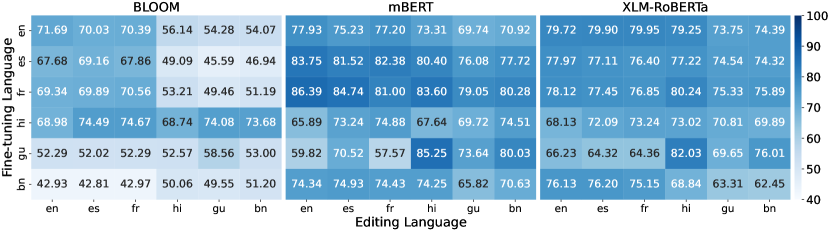
Figure 2: The figure illustrates $G_{S}$ given the editing language (x-axis) and fine-tuning languages (y-axis) for all the three models BLOOM (left), mBERT (middle) and XLM-RoBERTa (right) when edited using MEND.

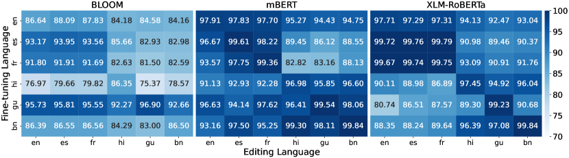
Figure 3: The figure illustrates $S_{S}$ given the editing language (x-axis) and fine-tuning languages (y-axis) for all the three models BLOOM (left), mBERT (middle) and XLM-RoBERTa (right) when edited using MEND.

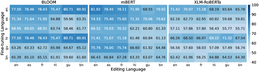
Figure 4: The figure illustrates $G_{S}$ given the editing language (x-axis) and fine-tuning languages (y-axis) for all the three models BLOOM (left), mBERT (middle) and XLM-RoBERTa (right) when edited using FT.

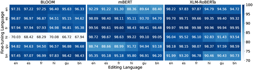
Figure 5: The figure illustrates $S_{S}$ given the editing language (x-axis) and fine-tuning languages (y-axis) for all the three models BLOOM (left), mBERT (middle) and XLM-RoBERTa (right) when edited using FT.

4.6 Experimental Settings

In our research methodology, we fine-tune the models described in Section 4.3 for each specific language. Following the fine-tuning process, we apply model editing techniques, as detailed in Section 4.4, by passing individual inputs to the fine-tuned models. The performance of these edited models is then evaluated using the metrics defined in Section 4.5.

To implement the Knowledge Editor and Fine-Tuning techniques, we utilize the implementation provided by MEND Mitchell et al. (2022a). Consistent with the experimental settings of MEND, we selectively update only four layers of each PLM. The same set of layers is updated by both KE and FT. For the decoder-only models, we designate layers 1–4 as initial layers (IL), 14–17 as middle layers (ML), 21–24 as last layers (LL), and we randomly select layers 9, 14, 18, and 22 as random layers (RL). Similarly, for the encoder-only models, we assign layers 1-4 as IL, 5–8 as ML, 9–12 as LL, and 3, 5, 7, and 10 as RL. We have utilized the default hyperparameters as implemented in the MEND’s implementation for MEND, KE, and FT. All experiments were completed on 4 V100 GPUs (Each consisting of 32GB).

5 Results

In this section, we present and analyze the key findings and address the research questions posed in Introduction Section (see Section 1 for more details). To accomplish this, we examine a total of 69 configurations, which are derived from combining six languages, three PLMs, and three METs. For each configuration, we present the results in tabular form. For instance, Table 1 showcases the performance measured by $G_{S}$ obtained from fine-tuning the mBERT (left) and BLOOM (right) on an en dataset and subsequently applying the MEND’s editing technique. The rows of the table represent the editing languages, while the columns represent the languages used for evaluation. The diagonal values represent monolingual $G_{S}$, whereas off-diagonal entries show cross-lingual $G_{S}$. Similarly, Table 2 showcases the performance measured by $S_{S}$ for mBERT when fine-tuned on en (left) and hi (right) and edited using MEND. In our experimental analysis, we observe consistent trends for both the MEND and KE techniques. However, due to space limitations, we focus on reporting the results obtained using the MEND approach. The performance scores for the KE technique can be found in §A.6. Next, we answer the posed research questions.

5.1 What is the effectiveness of hypernetwork-based editing techniques in cross-lingual settings?

Table 1 and 2 elucidates notable trends observed in evaluating existing METs. Table 1 demonstrates high values of $G_{S}$ (above 90%) along the diagonal entries, providing empirical evidence for the effectiveness of METs when applied to mBERT in monolingual contexts. Conversely, a noticeable decrease in the $G_{S}$ scores becomes evident as one moves away from the diagonal, indicating the relative inefficiency of METs in cross-lingual scenarios. Language pairs within the same script family, such as en$\rightarrow$es, en$\rightarrow$fr, or hi$\rightarrow$bn, achieve higher $G_{S}$ values compared to pairs belonging to different script families, such as en$\rightarrow$hi or es$\rightarrow$bn. The average $G_{S}$ (excluding the diagonal entries) for editing in the Latin family (90.04%) is significantly higher than in the Indic family (78.38%). However, the two branches do not significantly differ in the average $G_{S}$ under a monolingual setting. Similar trends are observed for fine-tuning mBERT in other languages (refer to §A.5.2, §A.6.2, and §A.7.2 for detailed results). Comparable patterns were also identified for XML-RoBERTa (refer to §A.5.3, §A.6.3, §A.7.3 for detailed results). The observations derived from the analysis of the BLOOM model reveal notable distinctions. The metric $G_{S}$ strongly depends on the fine-tuning language script, irrespective of the employed editing language. Specifically, when examining the en language, a significant disparity in $G_{S}$ values is observed between the Latin and Indic script families, as evident in Table 1. For instance, the average $G_{S}$ (including the diagonal entries) for the Latin and Indic families is 94.14% and 84.32%, respectively. Additional results pertaining to BLOOM can be found in §A.5.1, §A.6.1, and §A.7.1.

Unexpectedly, the $S_{S}$ metric presents contrasting findings compared to the $G_{S}$ metric. Encoder-only models’ $S_{S}$ mainly depend on the fine-tuning language script irrespective of the editing language. For example, in Table 2, average $S_{S}$ (including the diagonal entries) for the Latin family (97.63%) is sufficiently higher than Indic family (91.06%), when mBERT is finetuned on en. But when fine-tuned on hi, the average $S_{S}$ for Indic family (98.58%) is higher than the Latin family (85.85%). XLM-RoBERTa follows similar trends (See §A.5.3, §A.6.3, §A.7.3 for more details). In contrast, BLOOM shows a very distinct trend. It results in high $S_{S}$ for the Latin script family, irrespective of fine-tuning or editing language selection (refer §A.5.1, §A.6.1, and §A.7.1). Lastly, editing and verifying the edit in the same written script family yields better results.

Inference 1 In our analysis, let us consider that we fine-tune using the ‘en’ dataset, and later we perform the XME. If we look at Table 1, for BLOOM (right), the maximum GS for en-en is seen in the Middle layers (93.04%), while for the last layers, the reported GS is 85.83%. This shows that it is possible that the model stores the facts at different locations. Similarly, let us consider when we fine-tune using ‘en’ (In the same table) and edit and verify in Spanish (es-es); in this case, the reported GS is 89.1% in the middle layer and 87.26% in last layers. The information is significantly (different from nearly 2%) available across the sets of layers. We have extended the research question by exploring if the fine-tuning language also has any impact on the editing and if it shifts the information from the middle layers to other sets of layers.

Inference 2 Referring to Table 12, we fine-tune the BLOOM model on the ‘hi’ dataset. The GS score for hi-hi in the initial layer (92.37) is higher than the middle layers (85.58%), which tells us that when we fine-tuned the model on the Hindi dataset, the information is majorly stored in the initial layers rather than our previous assumption of middle layers.

5.2 Do different architectures store factual knowledge at different locations?

We have observed that different architectures store factual knowledge in distinct locations. Specifically, in the case of encoder-only models, a significant proportion of factual knowledge is found in the Last Layers (LL). Table 1 illustrates that the LL exhibits the highest average $G_{S}$ score (78.74%) compared to other layer sets (IL=70.23%, ML=77.93%, and RL=69.32%). In contrast, for BLOOM (decoder-based), factual knowledge is concentrated in the Middle Layers (ML). The ML achieves a notably higher average $G_{S}$ score (69.99%) than other layer sets (IL=61.16%, LL=59.19%, and RL=60.73%). This finding aligns with the observations made in (Meng et al., 2022a), which identified similar trends in GPT-2 (Radford et al., 2019), decoder-only model (Qi et al., 2023). Notably, the initial layers demonstrate the lowest $G_{S}$ scores for both encoder- and decoder-only models.

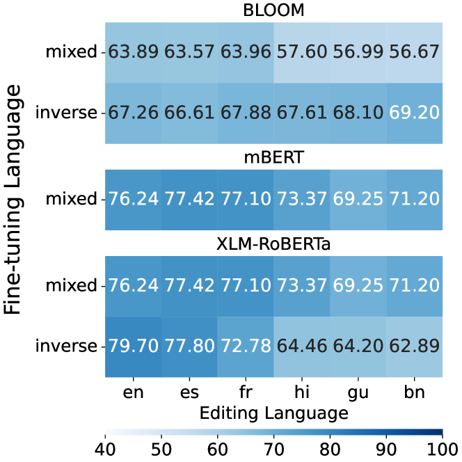
Figure 6: The figure illustrates $G_{S}$ given the editing language (x-axis) and fine-tuning datasets (y-axis) for all the three models BLOOM (top), mBERT (middle) and XLM-RoBERTa (right) when edited using MEND.

5.3 How does language selection in the initial fine-tuning affect editing performance?

Figure 2 shows the effect of initial fine-tuning performed using six languages. Columns represent average $G_{S}$ scores for each editing language. As illustrated, language selection during initial fine-tuning significantly impacts the editing performance for the decoder-only model BLOOM. For instance, fine-tuning on the Latin script family led to poor $G_{S}$ for the Indic script family. Similar trends can be observed when fine-tuning is performed on Indic script families. However, in the latter case, the difference of $G_{S}$ between the two families is not as high as observed in the former scenario. In the case of encoder-only models, we see a similar performance in both families for Latin scripts fine-tuning. In the case of Indic family fine-tuning, the performance of Latin scripts is marginally poor than that of Indic family. We attribute this to the effect of editing performance on the disproportionate pretraining on different languages.

We performed additional experiments involving two alternative fine-tuning settings. We created two snapshots of the fine-tuning data: (i) “mixed”, which contained an equal distribution of languages, and (ii) “inverse”, where the languages were represented inversely proportional to their respective pretraining language proportions. It is important to note that a single instance of the mixed dataset was generated for PLMs, while the inverse datasets were specific to each PLM. Since BLOOM and XLM-RoBERTa provide language representation information, we only created inverse datasets for these PLMs. Figure 6 illustrates the results obtained from the mixed and inverse datasets. Notably, the inverse dataset consistently exhibited performance improvements for the BLOOM model (aka decoder-based). However, the mixed fine-tuning approach performs poorly than the monolingual fine-tuning method. Lastly, in the case of encoder-only models, the mixed and inverse fine-tuning approaches decreased performance compared to the monolingual fine-tuning method.

Intriguingly, the $S_{S}$ metric reveals contrasting findings compared to the $G_{S}$ metric. Figure 3 demonstrates that the initial fine-tuning significantly impacts the $S_{S}$ scores of encoder-only models, whereas this observation is not observed for decoder-only models. Similarly, Figure 7 highlights that encoder-only models trained on the mixed dataset exhibit improved $S_{S}$ scores compared to monolingual fine-tuning. However, the mixed and inverse datasets do not result in any performance gain for the BLOOM model.

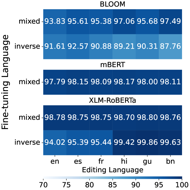
Figure 7: The figure illustrates $S_{S}$ given the editing language (x-axis) and fine-tuning datasets (y-axis) for all the three models BLOOM (top), mBERT (middle) and XLM-RoBERTa (right) when edited using MEND.

5.4 Is the traditional fine-tuning approach more effective than METs in achieving higher performance in the cross-lingual setting?

Figures  4 and  5 demonstrate that traditional fine-tuning approaches perform comparably to METs in cross-lingual settings. This observation contrasts the previous claim that shows the significantly low performance of METs in the monolingual setting (Xu et al., 2023; Meng et al., 2022a).

6 Conclusion and Future Directions

Our research focuses on conducting rigorous experiments with state-of-the-art hypernetwork-based model editing techniques within cross-lingual settings. Specifically, we investigate the storage patterns of factual associations in encoder-only and decoder-only models, using two distinct language families as our experimental basis. Additionally, we establish a clear dependency between the fine-tuning language selection and the editing tasks’ performance.

To further advance the XME paradigm, we plan to utilize parameter-preserving and localized editing techniques. Furthermore, we intend to extend our investigations to encompass other NLP tasks, such as Machine Translation or question-answering. By expanding our research, we aim to enhance our understanding of the capabilities and limitations of hypernetwork-based model editing techniques in diverse cross-lingual settings.

Limitations

The performance of METs including KN (Dai et al., 2022), SERAC (Mitchell et al., 2022b), CaliNet (Dong et al., 2022), Transformer-Patching (Murty et al., 2022), KAFT (Li et al., 2022), Patcher (Huang et al., 2023), is limited when the information is distributed across layers. Our experiments’ findings indicate that the information in different languages is dispensed across types of architectures. While our work focuses on encoder-based and decoder-based architectures, we intend to incorporate encoder-decoder architectures in future research. The objective is to enhance the localizing and efficient updating of factual information in tasks such as generation, translation, and others. To assess the cross-linguality in METs, we aim to propose a dataset to evaluate whether facts dependent on the edited information also undergo changes. For instance, does the fact ‘Where is the President of the USA’s hometown?’ also change when we edit the information about the ‘President of USA’.

Ethics and Potential Risks

The model-editing techniques are designed to edit or delete the information from the LLMs. The editing techniques can be used to modify the model’s parameters and can be adversely used. We do not show such harm and intend to show cross-lingual model editing. We carefully adhere to the ethics and guidelines and ensure our work is ethically correct.

MET	Model	en	fr	es	hi	gu	bn	mixed	inverse
MEND	BLOOM	9	10	11	12	13	14	15	16
	mBERT	17	18	19	20	21	22	23	-
	XLM-RoBERTa	24	25	26	27	28	29	30	31
KE	BLOOM	32	33	34	35	36	37	38	39
	mBERT	40	41	42	43	44	45	46	-
	XLM-RoBERTa	47	48	49	50	51	52	53	54
FT	BLOOM	55	56	57	58	59	60	61	62
	mBERT	63	64	65	66	67	68	69	-
	XLM-RoBERTa	70	71	72	73	74	75	76	77

Table 3: The table contains the index for all the configurations for ME techniques, models, and fine-tuning data.

Appendix A Appendix

This section contains all the $G_{S}$ and $S_{S}$ experiments using different ME techniques for different architectures.

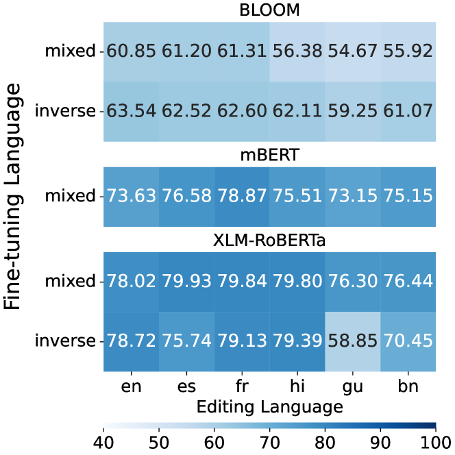
Figure 8: The figure illustrates $G_{S}$ given the editing language (x-axis) and fine-tuning datasets (y-axis) for all the three models BLOOM (top), mBERT (middle) and XLM-RoBERTa (right) when edited using KE.

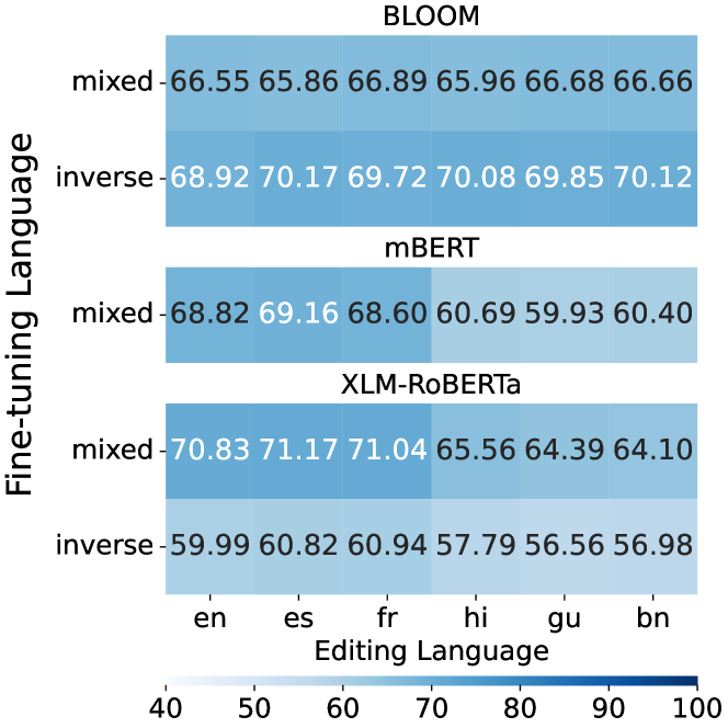
Figure 9: The figure illustrates $G_{S}$ given the editing language (x-axis) and fine-tuning datasets (y-axis) for all the three models BLOOM (top), mBERT (middle) and XLM-RoBERTa (right) when edited using FT.

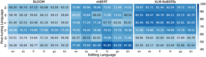
Figure 10: The figure illustrates $G_{S}$ given the editing language (x-axis) and fine-tuning languages (y-axis) for all the three models BLOOM (left), mBERT (middle) and XLM-RoBERTa (right) when edited using KE.

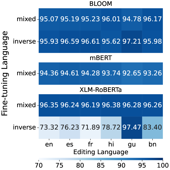
Figure 11: The figure illustrates $S_{S}$ given the editing language (x-axis) and fine-tuning datasets (y-axis) for all the three models BLOOM (top), mBERT (middle) and XLM-RoBERTa (right) when edited using KE.

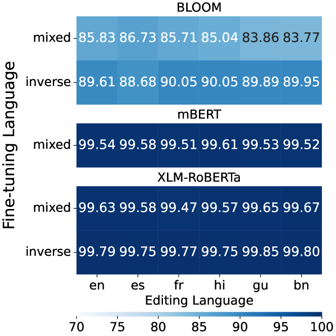
Figure 12: The figure illustrates $S_{S}$ given the editing language (x-axis) and fine-tuning datasets (y-axis) for all the three models BLOOM (top), mBERT (middle) and XLM-RoBERTa (right) when edited using FT.

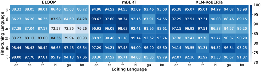
Figure 13: The figure illustrates $S_{S}$ given the editing language (x-axis) and fine-tuning languages (y-axis) for all the three models BLOOM (left), mBERT (middle) and XLM-RoBERTa (right) when edited using KE.

A.1 Dataset

The complete dataset statistic regarding the cross-lingual dataset and Average Lengths (AL) for encoder-only and decoder-only models are shown in Table 6. We considered the samples overlapping in all six languages (not including mixed and inverse) from the train, validation, and test splits. Table 7 and 8 report the inverse proportion of languages for BLOOM and XLM-RoBERTa.

A.2 Quality Assessment of Translations

We randomly selected 150 instances from the English-FEVER dataset (Thorne et al., 2018) and the corresponding translations and then assigned them to the human annotators. There were two annotators per language; each was a native speaker of the language assigned to them and proficient in English. We recruited language experts who voluntarily helped in the annotation process without pay.

Table 4 shows the individual annotation accuracy and inter-annotation agreement (IAA). In the table, the IAA column represents scores computed from Cohen’s Kappa coefficient, computed between two annotators for the respective language. While computing the IAA, annotators verified that the translated sentences were syntactically and semantically correct (No code-switching or code-mixing was allowed). Considering the Relaxed-IAA (R-IAA), code-mixed and code-switched transitions were assumed to be relaxed and surpassed (Correct semantics were verified). Further, $acc_{a1}$ and $acc_{a2}$ represent the accuracy of annotators one and two with strict instructions. Lastly, R-$acc_{a1}$ and R-$acc_{a2}$ represent the accuracy with the relaxed instructions from both annotators. Accuracy for individual annotators was over 80 percent in all the cases.

Language	IAA	R-IAA	$acc_{a1}$	$acc_{a2}$	Avg. Acc.	R-$acc_{a1}$	R-$acc_{a2}$	R-Avg. Acc.
French	67.00	80.00	88.67	94	91.33	92.00	93.33	92.66
Spanish	66.00	74.00	76.67	84.67	80.67	87.33	90.00	88.66
Hindi	63.00	85.00	75.33	76.67	76.00	93.33	92.67	93.00
Bengali	70.00	76.00	80.67	80.67	80.67	92.67	92.00	92.335
Gujarati	56.00	74.00	66.67	59.33	63.00	74.00	73.33	73.66
Average	64.4	77.8	77.60	79.07	78.33	87.87	88.27	88.07

Table 4: Inter-Annotator Agreement (IAA), Relaxed-IAA, and average accuracy per language the annotators assign for both standard and relaxed configurations (Reported numbers are percentages over 150 instances). In our experiments, two annotators represented as $a1$ and $a2$ were asked to annotate the correct translations. Standard accuracy per language by annotator is represented with $acc_{a1}$ and $acc_{a2}$, whereas relaxed accuracy is denoted with R-$acc_{a1}$ and R-$acc_{a2}$ for annotators one and two.

A.3 Model Editing Techniques

Table 5 reports the 24 editing techniques introduced in top venues over the recent years. The techniques are classified into different editing approaches. From the literature review, the editing techniques have gained popularity and trends to become a focused problem for the future never-aging LLMs. Figure 10 shows the average $G_{S}$ for all three models for KE. Furthermore, Figure 8 shows the mixed and inverse proportion results for the KE and FT. Similarly, Figures 13 and 5 show the average $S_{S}$ for all three models for KE and FT. Furthermore, Figure 11 and 12 shows the mixed and inverse proportion results for the KE and FT.

A.4 Implementation Details

We utilized the Mitchell et al. (2022a)’s implementation of MEND, KE, and FT. We used the default hyperparameters to fine-tune the base model and the MLPs as specified in MEND’s implementation. We edit one instance per batch. For all 69 configurations with Language Pairs x Models x METs, a total of 9,936 experiments were performed. From the tables indexed in 3, one experiment is computed as $G_{S}$ and $S_{S}$ for one configuration, say, in Table 9, for IL, when $x$ is en, and $x^{\prime}$ is en for both $G_{S}$ and $S_{S}$. Similarly, for one set of layers (36 values), there are a total of 4 sets and 69 configurations, which sums to 36 x 4 x 69 = 9,936 experiments.

A.5 MEND

A.5.1 BLOOM

Tables 9, 10, 11, 12, 13, 14, 15, and 16 shows the experiments on BLOOM when fine-tuned on en, fr, es, hi, gu, bn, mixed, and inverse, respectively using MEND.

A.5.2 mBERT

Tables 17, 18, 19, 20, 21, 22, and 23, shows the experiments on mBERT when fine-tuned on en, fr, es, hi, gu, bn, and mixed, respectively using MEND.

A.5.3 XLM-RoBERTa

Tables 24, 25, 26, 27, 28, 29, 30, and 31, shows the experiments on XLM-RoBERTa when fine-tuned on en, fr, es, hi, gu, bn, and mixed, respectively using MEND.

A.6 KE

A.6.1 BLOOM

Tables 32, 33, 34, 35, 36, 37, 38, and 39 shows the experiments on BLOOM when fine-tuned on en, fr, es, hi, gu, bn, mixed, and inverse, respectively using KE.

A.6.2 mBERT

Tables 40, 41, 42, 43, 44, 45, and 46, shows the experiments on mBERT when fine-tuned on en, fr, es, hi, gu, bn, and mixed, respectively using ke.

A.6.3 XLM-RoBERTa

Tables 47, 48, 49, 50, 51, 52, 53, and 54, shows the experiments on XLM-RoBERTa when fine-tuned on en, fr, es, hi, gu, bn, and mixed, respectively using MEND.

A.7 FT

A.7.1 BLOOM

Tables 55, 56, 57, 58, 59, 60, 61, and 62 shows the experiments on BLOOM when fine-tuned on en, fr, es, hi, gu, bn, mixed, and inverse, respectively using FT.

A.7.2 mBERT

Tables 40, 41, 42, 43, 44, 45, and 46, shows the experiments on mBERT when fine-tuned on en, fr, es, hi, gu, bn, and mixed, respectively using FT.

A.7.3 XLM-RoBERTa

Tables 70, 71, 72, 73, 74, 75, 76, and 77, shows the experiments on XLM-RoBERTa when fine-tuned on en, fr, es, hi, gu, bn, and mixed, respectively using FT.

All 69 configurations for ME techniques, models, and languages are indexed to Table 3. The normalized $G_{S}$ for KE and FT are shown in Figure 10 and 4, respectively. Furthermore, Figures 8 and 9 show the normalized $G_{S}$ for KE and FT for mixed and inverse configurations, respectively using MEND.

Technique	Venue	On Arxiv	Cit.	Technique	Code
ENNs (Sinitsin et al., 2020)	ICLR 20’	Apr 01, 2020	76	LE	Y
KE (De Cao et al., 2021)	EMNLP 21’	Apr 16, 2021	75	HN	Y
KN (Dai et al., 2022)	ACL Proceeding 22’	Apr 18, 2021	75	HN	Y
CuQA (Lee et al., 2022)	ACL Proceeding 22’	Apr 22, 2021	1	LE	Y
MEND (Mitchell et al., 2022a)	ICLR 22’	Oct 21, 2021	73	HN	-
SLAG (Hase et al., 2021)	Arxiv	Nov 26, 2021	21	LE	Y
Editing-classifier (Santurkar et al., 2021)	NeurIPS 21’	Dec 01, 2021	30	LE	Y
FRUIT (Iv et al., 2022)	NAACL 22’	Dec 16, 2022	5	-	-
Prompt-editing (Madaan et al., 2022)	EMNLP 22’	Jan 16, 2022	8	PP	Y
ROME (Meng et al., 2022a)	NeurIPS 22’	Feb 10, 2022	38	LE	Y
FactTracing (Akyurek et al., 2022)	EMNLP	May 23, 2022	2	-	Y
SERAC (Mitchell et al., 2022b)	ICML 22’	June 13, 2022	14	PP	Y
RepairNN (Tanno et al., 2022)	Arxiv	July 11, 2022	-	LE	-
PAINT (Ilharco et al., 2022)	NeurIPS 22’	Aug 10, 2022	19	-	Y
CaliNet (Dong et al., 2022)	EMNLP 22’	Oct 07, 2022	1	PP	Y
MEMIT (Meng et al., 2022b)	ICLR 23’	Oct 13, 2022	9	LE	Y
Entailer (Tafjord et al., 2022)	EMNLP 22’	Oct 21, 2022	5	-	Y
GRACE (Hartvigsen et al., 2022)	NeurIPS 22’	Nov 20, 2022	-	LE	-
Cross-lingual (Xu et al., 2023)	Arxiv	May 25, 2022	2	LE	-
Prompting (Si et al., 2023)	ICLR 23’	Oct 17, 2022	8	-	Y
Transformer-Patching (Murty et al., 2022)	EMNLP 22’	Nov 07, 2022	3	PP	Y
KAFT (Li et al., 2022)	Arxiv	Nov 09, 2022	5	PP	-
LocalizedEdit (Hase et al., 2023)	Arxiv	Jan 10, 2023	1	LE	Y
Patcher (Huang et al., 2023)	ICLR 23’	Jan 23, 2023	-	PP	Y

Table 5: Recent works in METs. Note: Citations were last reported on April 11, 2023. Here, PP stands for ‘Parameter Preserving,’ HN for ‘HyperNetworks,’ and LE for ‘Localized Edits.’

Lang	ALα	ALβ	ALγ	Train	TFR	VFR
en	11.25	10.67	11.87	104966	10.9998	10.5003
hi	14.4	18.04	15.69	103191	10.691	10.2668
es	12.25	12.53	14.07	104965	10.8479	10.3747
fr	10.5	10.6	12.79	104966	10.8479	10.3529
bn	13.58	20.72	17.61	104966	10.8479	10.3747
gu	15.93	23.86	18.07	104966	10.8479	10.3747
mix	11.25	10.67	11.25	102922	10.8633	10.4186
$Inv_{bloom}$	11.25	-	-	104504	10.8437	10.3747
$Inv_{xlm}$	-	-	11.95	104966	10.8483	10.3747

Table 6: Dataset statistics in different languages. Note TFR and VFR are the average length of training-filtered and validation filtered rephrases, respectively. $Inv_{bloom}$ and $Inv_{xlm}$ are the inverse proportion of BLOOM and XLM-RoBERTa. We do not include the inverse proportion of mBERT. Lastly, in all the languages, the size of validation and test remains 10444 and 1193, respectively.

Language	Size (x$10^{10}$)	Proportion (In %)	Inv. Proportion	Train	Test
en	48.50	53.13	1.88	230	23
fr	20.82	22.82	4.38	536	53
es	17.50	19.18	5.21	638	63
hi	2.46	2.7	37.07	4534	451
gu	1.86	2.04	49.05	6000	597
bn	0.12	0.13	760.61	93029	9256
Total	91.27	1	858.21	104967	10443

Table 7: Statistics of inverse proportion dataset for BLOOM. The dataset is prepared while considering the portion of languages at the pre-training stage. Proportion is shown in percentage over the six languages.

Language	Size (x$10^{3}$)	Proportion (In %)	Inv. Proportion	Train	Test
en	55.6	72.09	1.39	191	19
fr	9.78	12.68	7.89	1089	108
es	9.37	12.15	8.23	1136	113
hi	1.71	2.22	44.98	6209	618
gu	0.53	0.68	146.93	20282	2018
bn	0.14	0.18	551.01	76059	7568
Total	77.14	1	760.44	104966	10444

Table 8: Statistics of inverse proportion dataset for xlm-roberta. The dataset is prepared while considering the portion of languages at the pre-training stage. Proportion is shown in percentage over the six languages.

		$G_{S}$ ($x^{\prime}$) $\rightarrow$						$S_{S}$ ($\hat{x}$) $\rightarrow$
Set	$x$ $\downarrow$	en	fr	es	hi	gu	bn	en	fr	es	hi	gu	bn
IL	en	87.93	79.8	80.72	59.93	48.37	58.26	96.5	96.96	96.75	86.61	92.98	87.66
	fr	76.36	87.43	81.81	58.26	49.29	56.92	97.65	96.94	97.17	88.14	94.74	88.92
	es	77.03	80.81	87.68	59.51	48.37	56.16	97.02	97.32	95.79	86.9	95.37	89.19
	hi	50.88	52.89	52.98	65.8	48.7	58.26	98.83	99.12	99.08	74.77	93.84	80.89
	gu	50.46	51.63	51.97	53.06	51.47	57.59	99.31	99.48	99.54	89.19	85.86	82.33
	bn	49.96	51.8	51.55	53.56	49.04	65.55	99.04	99.33	99.27	87.59	93.27	75.08
ML	en	93.04	90.7	88.77	65.55	54.99	69.32	96.02	95.31	95.18	51.57	61.46	57.59
	fr	86.17	89.69	88.27	64.46	54.57	66.97	96.88	95.41	95.89	52.24	61.42	57.63
	es	85.41	89.44	89.1	64.21	54.82	65.72	96.81	95.7	95.91	52.37	61.46	57.75
	hi	55.41	59.35	58.26	74.1	70.16	75.27	97.44	96.48	96.77	56.6	59.91	59.01
	gu	55.49	57.75	56.92	73.6	62.7	76.61	97.51	96.35	96.65	52.22	57.82	59.22
	bn	53.9	56.66	55.57	72.42	73.26	71.08	97.38	96.42	96.79	56.08	58.21	59.16
LL	en	85.83	78.79	79.97	58.09	48.53	63.2	95.96	96.77	96.1	79.97	83.51	75.0
	fr	65.97	89.19	78.21	59.26	48.7	64.46	97.9	97.02	97.74	83.97	88.66	78.96
	es	64.46	74.94	87.26	60.86	49.04	66.55	97.82	98.13	97.32	84.6	90.78	81.03
	hi	53.06	53.48	53.9	43.59	48.45	49.2	98.01	98.41	98.18	60.12	75.0	65.3
	gu	51.21	53.14	52.98	50.71	50.29	45.52	98.66	98.95	98.81	71.81	49.37	61.42
	bn	52.72	54.15	53.4	46.19	47.86	47.53	98.28	98.39	98.24	67.6	71.84	50.67
RL	en	88.94	85.83	85.75	54.32	51.05	62.95	96.08	96.29	96.14	80.13	92.83	76.05
	fr	82.31	88.35	85.16	53.4	52.64	61.44	96.75	94.93	96.25	80.53	94.28	77.89
	es	80.97	82.73	87.85	53.06	53.56	61.27	97.25	97.0	95.81	80.16	93.71	78.98
	hi	53.81	56.75	56.5	51.72	52.98	51.89	98.2	98.39	98.32	63.37	86.13	68.06
	gu	54.15	56.92	56.33	54.23	32.86	45.1	98.68	99.14	98.91	86.5	66.26	86.0
	bn	53.81	56.08	55.91	41.99	45.77	37.8	98.49	98.93	98.74	72.88	88.39	59.68

Table 9: The table represents the $G_{S}$ and $S_{S}$ using MEND over fine-tuned BLOOM on the fever ‘en’ dataset.

		$G_{S}$ ($x^{\prime}$) $\rightarrow$						$S_{S}$ ($\hat{x}$) $\rightarrow$
Set	$x$ $\downarrow$	en	fr	es	hi	gu	bn	en	fr	es	hi	gu	bn
IL	en	80.22	71.42	75.11	51.89	55.66	54.4	92.69	93.17	91.53	69.09	62.01	63.77
	fr	71.75	79.46	74.94	52.56	56.08	54.57	92.69	93.46	91.53	64.48	58.53	59.03
	es	69.74	70.49	82.15	53.98	57.42	54.74	92.92	92.9	91.62	67.52	63.66	62.61
	hi	53.81	53.56	53.73	49.71	46.61	42.92	93.48	92.73	91.53	48.18	58.93	55.89
	gu	52.47	51.89	53.48	39.82	46.19	46.61	92.67	92.94	91.79	66.68	44.51	61.84
	bn	51.89	51.97	52.56	48.45	46.27	43.17	93.67	93.5	93.13	63.5	58.28	58.68
ML	en	95.56	96.06	96.48	54.32	50.8	54.9	97.05	98.28	97.9	92.69	97.32	95.01
	fr	95.47	98.24	97.15	54.99	52.05	55.41	99.2	99.06	98.93	93.75	97.82	95.35
	es	94.22	96.14	97.23	54.65	52.05	56.41	99.45	99.18	99.02	93.38	97.9	95.47
	hi	61.19	62.28	63.37	49.96	50.29	54.57	98.93	99.2	99.08	73.53	84.95	78.62
	gu	56.41	57.33	58.68	48.62	31.1	51.72	99.1	98.83	98.26	78.71	60.39	80.01
	bn	57.0	58.76	58.84	59.43	52.56	53.56	98.49	98.2	98.01	76.32	80.34	70.08
LL	en	96.98	94.47	91.79	54.23	48.37	58.0	99.1	99.52	99.43	94.91	98.05	96.25
	fr	91.79	97.9	93.97	54.06	48.45	60.52	99.75	99.48	99.43	94.32	97.57	96.0
	es	86.34	93.04	96.65	54.82	48.28	59.93	99.58	99.62	99.33	95.14	98.43	97.13
	hi	56.33	57.59	59.09	44.43	64.38	59.68	98.01	98.45	98.26	46.1	75.06	68.8
	gu	52.81	53.4	52.56	52.39	31.77	45.6	96.1	96.0	95.66	63.14	56.89	70.6
	bn	53.98	54.9	54.32	46.1	49.2	43.92	97.78	98.18	97.4	66.34	74.62	51.99
RL	en	93.8	88.77	87.09	28.25	48.28	37.3	98.6	98.99	98.78	83.36	97.11	88.7
	fr	92.46	96.73	92.54	31.6	49.37	41.41	98.93	98.45	98.91	85.31	96.69	91.91
	es	89.94	92.04	94.64	32.94	49.79	39.73	98.95	98.97	98.43	79.74	96.67	88.2
	hi	59.18	58.93	59.01	32.36	47.28	36.88	96.19	96.33	95.73	64.42	90.82	79.78
	gu	60.52	62.61	59.43	43.25	31.69	46.69	95.22	95.62	94.59	78.56	69.74	78.14
	bn	56.08	55.24	55.32	40.74	45.43	38.98	96.06	95.91	95.45	76.57	83.68	65.91

Table 10: The table represents the $G_{S}$ and $S_{S}$ using MEND over fine-tuned BLOOM on the fever ‘fr’ dataset.

		$G_{S}$ ($x^{\prime}$) $\rightarrow$						$S_{S}$ ($\hat{x}$) $\rightarrow$
Set	$x$ $\downarrow$	en	fr	es	hi	gu	bn	en	fr	es	hi	gu	bn
IL	en	83.4	72.84	74.52	41.24	45.85	52.05	96.84	95.45	94.26	71.96	81.98	64.38
	fr	71.58	77.62	74.94	40.99	45.68	52.22	97.21	95.22	93.88	71.46	81.96	64.65
	es	73.68	72.25	84.91	40.32	46.35	52.22	96.81	95.39	93.69	71.5	81.94	64.9
	hi	52.72	52.56	52.22	39.31	47.7	31.94	95.85	95.08	94.64	81.75	81.94	64.69
	gu	55.99	55.49	55.32	34.03	31.77	46.02	94.01	94.47	94.11	85.39	65.97	64.08
	bn	52.81	52.56	52.14	43.42	46.27	32.02	96.29	95.49	95.2	80.68	83.07	61.88
ML	en	94.8	92.37	93.63	52.3	47.11	53.06	97.13	98.53	98.3	94.53	98.05	92.22
	fr	86.67	95.47	93.46	53.9	48.7	53.31	98.68	98.47	98.51	94.91	98.45	92.85
	es	89.27	93.38	96.9	55.41	49.87	53.23	98.93	98.83	98.81	94.99	98.39	92.92
	hi	53.56	54.06	56.33	55.16	52.22	49.37	94.87	95.98	96.1	80.05	84.81	72.46
	gu	54.99	55.66	57.92	30.59	19.03	36.88	93.92	95.81	95.83	84.85	60.5	75.08
	bn	50.8	51.05	53.81	52.81	45.52	39.48	94.3	94.28	94.41	75.15	79.59	64.38
LL	en	94.3	82.15	81.22	45.18	46.52	40.23	97.46	98.09	98.64	93.34	98.78	87.24
	fr	80.64	92.54	82.31	45.1	45.77	45.26	98.95	97.92	99.12	92.83	98.47	90.23
	es	80.05	86.42	96.73	46.19	46.86	47.86	99.48	99.31	99.37	93.15	99.35	94.07
	hi	54.06	54.06	54.32	16.76	44.17	48.28	97.84	95.64	93.8	55.13	83.24	63.77
	gu	53.81	53.06	55.24	36.71	8.21	27.74	95.47	95.24	95.22	78.71	50.73	53.88
	bn	54.06	53.4	55.32	36.46	41.91	29.09	97.32	94.47	92.83	70.31	68.04	55.3
RL	en	97.65	97.23	96.73	44.59	40.49	54.74	98.74	98.74	98.93	91.45	98.45	92.52
	fr	96.56	98.41	97.57	49.45	43.09	57.42	99.22	98.7	99.27	91.64	98.64	94.22
	es	97.57	98.66	98.83	51.3	44.59	57.0	99.27	99.33	99.12	92.75	98.53	93.9
	hi	56.08	56.08	56.08	41.58	48.28	51.3	98.09	96.33	94.47	76.38	90.34	72.53
	gu	63.7	63.87	65.21	45.43	34.45	52.98	97.95	96.0	94.47	85.14	64.35	79.04
	bn	58.34	57.08	57.33	42.92	34.2	33.86	97.65	96.21	95.12	71.98	79.46	58.03

Table 11: The table represents the $G_{S}$ and $S_{S}$ using MEND over fine-tuned BLOOM on the fever ‘es’ dataset.

		$G_{S}$ ($x^{\prime}$) $\rightarrow$						$S_{S}$ ($\hat{x}$) $\rightarrow$
Set	$x$ $\downarrow$	en	fr	es	hi	gu	bn	en	fr	es	hi	gu	bn
IL	en	82.31	78.79	78.37	59.77	53.14	58.26	64.48	68.42	67.48	84.37	74.1	74.12
	fr	83.49	87.85	86.5	62.45	56.66	60.02	73.68	68.13	71.71	88.01	79.19	78.14
	es	82.98	86.34	86.84	62.87	57.08	61.78	73.45	70.62	67.31	87.66	79.23	78.06
	hi	53.98	54.9	56.58	92.37	54.57	72.17	91.01	89.8	90.17	90.88	91.39	82.98
	gu	52.14	58.09	58.26	73.34	77.28	81.06	84.45	76.32	78.0	79.36	37.26	46.44
	bn	51.63	54.82	55.83	74.43	89.69	91.87	88.6	82.86	84.22	81.96	51.03	51.93
ML	en	73.18	60.86	60.6	60.35	50.8	65.05	73.85	79.57	79.44	86.17	81.06	78.04
	fr	65.8	67.9	65.46	67.06	61.36	79.88	84.95	85.2	85.79	90.26	84.89	79.99
	es	65.72	65.21	67.56	65.13	62.03	79.46	84.68	85.86	85.9	90.55	84.62	79.42
	hi	55.99	58.84	58.93	85.58	59.51	87.93	92.44	90.17	90.09	85.44	88.18	78.65
	gu	55.91	60.94	63.37	73.76	92.2	97.4	86.25	83.72	82.44	88.14	64.73	66.09
	bn	54.4	59.35	59.09	75.86	86.84	98.58	91.28	87.39	87.55	85.98	71.42	66.22
LL	en	84.07	73.76	74.6	69.49	59.77	77.79	73.39	75.11	75.36	85.23	74.08	73.39
	fr	78.54	85.67	83.4	77.37	75.52	86.17	78.46	74.77	74.92	85.88	75.02	74.16
	es	76.03	82.4	85.41	76.61	76.03	87.26	78.25	75.27	74.58	85.94	75.0	74.16
	hi	65.55	71.84	72.51	90.95	69.41	94.05	86.23	79.4	78.65	81.16	76.59	71.42
	gu	65.46	75.94	77.2	78.12	94.13	97.48	81.41	75.06	75.08	88.79	65.0	68.15
	bn	64.71	73.68	74.43	78.21	91.2	98.16	86.84	80.05	79.95	87.17	67.81	66.2
RL	en	78.71	73.85	73.93	68.9	61.44	77.7	74.27	79.0	79.82	83.4	84.12	79.15
	fr	69.49	81.14	79.88	72.67	69.99	87.76	77.49	77.43	78.35	90.4	81.12	77.62
	es	70.58	77.95	81.81	71.67	70.58	88.35	77.24	77.64	78.12	90.26	80.51	77.45
	hi	52.14	51.13	51.8	86.67	60.1	92.29	90.13	93.65	93.0	89.14	89.82	81.94
	gu	52.64	62.61	64.8	76.87	93.13	95.81	88.92	84.97	83.93	90.74	64.92	68.67
	bn	50.29	59.77	60.94	75.36	89.86	99.33	85.75	87.55	86.46	90.91	67.5	69.01

Table 12: The table represents the $G_{S}$ and $S_{S}$ using MEND over fine-tuned BLOOM on the fever ‘hi’ dataset.

		$G_{S}$ ($x^{\prime}$) $\rightarrow$						$S_{S}$ ($\hat{x}$) $\rightarrow$
Set	$x$ $\downarrow$	en	fr	es	hi	gu	bn	en	fr	es	hi	gu	bn
IL	en	54.99	54.82	54.9	49.29	48.53	54.15	99.92	99.92	99.81	95.6	96.81	95.49
	fr	55.57	55.41	55.41	49.79	48.28	54.4	99.92	99.89	99.83	95.66	96.92	95.68
	es	54.32	54.23	54.32	49.04	48.28	53.14	100.0	99.98	99.87	95.68	97.05	95.79
	hi	52.22	52.3	52.39	62.53	53.9	52.81	100.0	99.98	99.89	94.05	96.96	95.94
	gu	52.14	52.22	52.14	52.89	88.35	54.99	100.0	99.98	99.92	96.08	96.31	95.08
	bn	51.55	51.8	51.72	50.29	53.4	54.9	99.69	99.75	99.56	95.18	97.13	93.82
ML	en	54.65	54.4	54.48	65.72	51.63	60.27	99.75	99.75	99.67	92.12	87.87	94.74
	fr	53.81	54.06	53.98	63.7	52.22	58.76	99.81	99.69	99.69	93.23	87.61	95.24
	es	53.73	53.65	53.9	64.21	51.72	58.59	99.96	99.92	99.81	93.4	87.61	95.81
	hi	52.3	52.39	52.39	68.06	58.34	56.33	100.0	99.98	99.96	76.47	91.66	90.63
	gu	52.05	52.05	52.05	66.97	91.03	54.99	100.0	100.0	99.87	90.86	94.43	93.23
	bn	51.8	52.05	51.89	73.85	59.68	60.02	99.79	99.81	99.71	82.8	92.9	87.8
LL	en	52.05	52.05	52.05	35.88	42.83	50.13	99.96	99.96	99.81	80.85	73.66	93.02
	fr	52.05	52.05	52.05	36.46	43.59	50.96	99.98	99.96	99.81	79.27	70.6	91.91
	es	52.05	52.05	52.05	35.79	43.84	51.47	99.98	99.96	99.81	79.9	71.88	92.92
	hi	52.05	52.05	52.05	25.23	55.57	34.95	99.94	99.96	99.73	53.65	84.51	73.95
	gu	52.05	52.05	52.05	39.15	68.57	51.8	99.98	100.0	99.85	93.13	80.51	94.59
	bn	52.05	52.05	52.05	34.79	59.51	38.14	99.89	99.96	99.81	55.09	77.22	73.89
RL	en	52.64	52.64	52.64	54.32	47.28	52.72	99.89	99.81	99.83	95.7	95.89	97.74
	fr	52.39	52.3	52.47	54.65	47.86	52.64	99.83	99.79	99.79	95.64	95.7	97.63
	es	52.47	52.47	52.47	54.48	47.61	52.47	100.0	99.98	99.89	96.25	96.48	97.63
	hi	51.97	51.97	52.05	62.61	55.41	49.71	99.98	99.96	99.94	69.32	94.57	93.36
	gu	52.05	52.05	52.05	62.2	94.38	55.07	100.0	100.0	99.98	96.96	97.23	97.63
	bn	52.14	52.14	52.05	66.3	55.32	42.58	99.94	99.98	99.96	89.65	95.56	85.06

Table 13: The table represents the $G_{S}$ and $S_{S}$ using MEND over fine-tuned BLOOM on the fever ‘gu’ dataset.

		$G_{S}$ ($x^{\prime}$) $\rightarrow$						$S_{S}$ ($\hat{x}$) $\rightarrow$
Set	$x$ $\downarrow$	en	fr	es	hi	gu	bn	en	fr	es	hi	gu	bn
IL	en	55.07	54.9	54.23	50.8	46.27	47.44	99.85	99.87	99.89	94.36	98.49	97.11
	fr	54.99	55.32	54.65	48.79	45.01	45.68	99.96	99.98	99.98	94.13	98.45	97.25
	es	55.16	55.16	55.49	49.45	45.18	46.02	99.94	99.96	99.94	93.86	98.34	97.17
	hi	52.39	52.39	52.39	80.97	47.78	51.63	100.0	100.0	100.0	78.16	96.35	96.58
	gu	53.48	53.06	53.23	50.71	58.76	50.8	99.85	99.81	99.83	92.75	78.19	95.24
	bn	52.05	52.05	52.05	53.23	48.7	82.31	100.0	100.0	100.0	95.05	98.68	97.25
ML	en	54.06	54.32	54.4	56.92	44.84	47.95	99.69	99.71	99.73	97.15	97.69	96.92
	fr	53.73	54.48	54.74	56.33	44.76	49.12	99.73	99.77	99.71	97.69	98.18	97.59
	es	52.47	53.06	53.56	57.67	45.43	48.62	99.92	99.98	99.96	97.63	98.11	97.23
	hi	52.14	52.14	52.14	89.69	48.03	66.89	100.0	100.0	100.0	79.21	98.49	98.83
	gu	52.14	52.14	51.97	66.64	69.15	65.46	100.0	100.0	100.0	92.9	74.27	94.87
	bn	52.05	52.05	52.05	72.92	48.53	92.96	100.0	100.0	100.0	97.38	99.16	99.02
LL	en	10.56	13.91	14.33	9.05	0.75	53.48	47.97	48.3	48.32	56.87	65.21	32.5
	fr	11.99	10.73	12.32	12.49	1.76	55.91	47.99	48.01	48.03	58.4	65.8	32.48
	es	11.82	11.82	9.64	10.23	1.51	56.16	48.2	48.09	48.03	58.07	65.38	32.38
	hi	19.78	21.21	20.03	25.06	25.48	28.08	45.18	43.34	42.08	49.35	50.29	59.89
	gu	30.34	30.76	31.01	24.81	19.78	31.35	41.49	41.41	40.26	51.28	48.22	57.67
	bn	16.76	18.02	15.42	33.03	30.51	32.86	43.34	42.92	41.6	50.5	49.6	64.88
RL	en	52.39	52.14	52.3	55.07	45.77	49.37	99.87	99.89	99.89	97.38	98.2	98.53
	fr	52.56	52.47	52.64	55.49	45.52	49.79	99.83	99.85	99.83	97.9	98.22	98.62
	es	52.56	52.56	52.64	54.99	46.19	50.04	100.0	100.0	100.0	98.11	98.37	98.62
	hi	52.39	52.14	52.14	90.03	49.04	67.56	99.98	100.0	100.0	87.7	98.62	98.99
	gu	52.14	52.14	52.22	63.2	60.86	63.03	99.98	100.0	100.0	97.02	89.59	97.38
	bn	52.05	52.05	52.05	71.42	48.95	94.8	99.98	100.0	100.0	98.22	99.22	99.2

Table 14: The table represents the $G_{S}$ and $S_{S}$ using MEND over fine-tuned BLOOM on the fever ‘bn’ dataset.

		$G_{S}$ ($x^{\prime}$) $\rightarrow$						$S_{S}$ ($\hat{x}$) $\rightarrow$
Set	$x$ $\downarrow$	en	fr	es	hi	gu	bn	en	fr	es	hi	gu	bn
IL	en	76.19	69.32	70.75	52.47	47.95	50.54	94.07	95.77	94.91	91.2	95.73	91.34
	fr	71.67	79.3	74.6	51.05	48.2	49.87	95.37	94.61	94.17	92.22	96.33	92.5
	es	70.16	71.75	75.02	51.3	47.78	50.29	95.18	95.62	94.11	91.7	96.63	92.73
	hi	52.56	53.81	53.81	72.51	48.11	55.16	99.06	99.25	98.95	94.36	98.28	96.35
	gu	49.87	52.22	52.3	52.56	62.03	53.06	99.39	99.69	99.39	96.31	86.59	96.5
	bn	50.96	52.56	53.31	55.41	48.03	73.34	99.25	99.54	99.33	96.17	97.67	95.08
ML	en	87.34	84.74	84.07	56.33	48.11	56.75	93.29	95.35	95.01	88.92	91.32	89.1
	fr	81.98	87.59	85.0	55.24	48.53	54.23	96.1	96.4	96.5	91.87	94.59	92.48
	es	82.65	85.75	88.18	57.33	48.79	55.57	95.91	96.69	96.14	92.77	94.78	92.79
	hi	52.22	54.32	53.98	82.98	48.28	67.48	99.31	99.54	99.56	90.61	99.1	94.89
	gu	50.96	52.3	51.8	54.82	79.55	56.33	99.1	99.58	99.54	97.53	79.25	97.61
	bn	50.96	52.64	52.72	64.96	48.45	80.05	99.35	99.5	99.5	94.47	98.87	91.49
LL	en	80.97	65.97	65.46	51.3	48.62	54.06	91.85	94.78	95.41	92.75	95.1	93.19
	fr	68.57	82.48	65.72	51.3	48.87	53.4	95.03	93.61	96.69	95.31	96.94	95.62
	es	62.78	64.54	76.95	51.63	48.87	53.56	96.4	97.36	95.66	95.77	96.67	95.83
	hi	51.38	52.89	52.64	74.6	48.2	60.1	99.18	99.33	99.22	85.88	99.29	94.61
	gu	50.38	52.64	52.3	53.4	89.02	57.75	99.5	99.54	99.41	97.65	79.36	97.02
	bn	50.71	52.72	51.97	59.18	48.2	73.68	99.12	99.33	99.33	94.66	99.02	89.23
RL	en	87.43	68.57	70.91	53.56	48.2	53.65	93.97	96.75	96.71	94.57	96.48	94.41
	fr	69.15	85.58	70.33	53.14	48.62	50.63	96.84	96.88	97.74	96.96	98.16	96.25
	es	69.49	69.41	88.27	54.23	48.28	53.06	97.0	98.01	96.77	96.42	97.44	96.33
	hi	52.05	53.14	53.4	80.55	48.37	59.85	99.5	99.69	99.58	87.07	99.56	97.3
	gu	50.21	52.05	52.3	52.98	84.07	52.81	99.58	99.77	99.58	98.45	77.98	98.07
	bn	50.21	52.47	51.89	58.84	48.37	78.46	99.64	99.83	99.69	97.3	99.56	92.79

Table 15: The table represents the $G_{S}$ and $S_{S}$ using MEND over fine-tuned BLOOM on the fever ‘mixed’ dataset.

		$G_{S}$ ($x^{\prime}$) $\rightarrow$						$S_{S}$ ($\hat{x}$) $\rightarrow$
Set	$x$ $\downarrow$	en	fr	es	hi	gu	bn	en	fr	es	hi	gu	bn
IL	en	80.81	75.78	72.59	69.15	72.76	69.57	85.06	86.04	87.97	91.87	88.62	91.64
	fr	77.79	82.06	73.18	70.41	72.92	71.5	84.89	85.6	87.8	91.74	87.13	91.14
	es	76.53	77.2	77.28	67.31	70.49	67.06	86.21	87.51	88.94	93.88	87.95	94.03
	hi	74.85	75.78	68.23	78.71	72.17	77.28	80.85	80.36	86.19	80.55	88.37	78.27
	gu	76.7	76.95	73.26	70.16	84.49	70.41	84.03	85.67	85.73	92.58	86.5	92.98
	bn	76.28	75.69	68.57	84.07	72.42	85.33	80.07	79.8	85.46	79.97	88.64	76.7
ML	en	61.27	58.68	58.17	57.75	58.59	57.92	95.85	96.21	96.27	96.1	95.08	96.48
	fr	59.35	60.86	58.51	58.76	58.51	58.51	94.68	96.25	96.0	95.26	95.22	95.79
	es	59.85	59.51	61.86	56.16	59.26	55.99	95.35	96.63	96.04	96.96	95.83	97.65
	hi	59.93	58.51	57.17	61.36	60.1	60.27	93.34	94.55	95.54	92.58	94.45	93.36
	gu	59.77	60.18	59.35	57.75	68.06	57.33	92.16	93.46	92.22	94.15	91.45	95.05
	bn	59.35	59.26	56.66	63.7	59.6	63.37	92.79	93.46	95.03	90.38	94.07	91.45
LL	en	71.75	68.9	65.63	64.38	66.72	64.04	90.51	91.16	92.16	92.18	90.61	92.54
	fr	68.82	73.51	66.47	65.8	66.39	65.46	89.77	90.53	91.7	90.57	90.11	91.22
	es	69.57	69.24	72.34	61.53	67.06	60.86	90.82	91.85	92.46	93.8	90.82	94.13
	hi	66.64	67.9	63.96	72.0	69.49	69.07	89.82	90.67	93.11	87.28	91.45	88.01
	gu	67.98	68.73	65.13	65.8	79.38	65.46	88.35	89.44	90.15	90.42	88.45	91.34
	bn	65.88	68.23	61.27	72.0	67.39	76.11	89.56	89.17	92.48	85.33	91.72	85.71
RL	en	78.96	73.34	70.08	63.54	68.82	65.13	88.56	89.06	90.53	92.46	90.44	91.16
	fr	72.59	78.46	70.91	64.96	68.65	64.63	87.49	88.47	90.09	90.82	89.06	89.88
	es	72.0	72.67	76.61	60.52	67.14	60.6	89.77	90.8	91.72	94.36	90.55	93.53
	hi	69.32	68.82	67.14	69.82	69.74	64.38	88.6	89.84	91.97	90.63	90.32	90.95
	gu	67.06	67.48	65.97	62.28	82.06	62.61	88.29	89.77	89.88	92.81	89.0	93.61
	bn	71.17	71.17	65.63	69.91	69.82	77.79	85.92	86.78	89.92	87.01	88.89	85.98

Table 16: The table represents the $G_{S}$ and $S_{S}$ using MEND over fine-tuned BLOOM on the fever ‘inverse’ dataset.

		$G_{S}$ ($x^{\prime}$) $\rightarrow$						$S_{S}$ ($\hat{x}$) $\rightarrow$
Set	$x$ $\downarrow$	en	fr	es	hi	gu	bn	en	fr	es	hi	gu	bn
IL	en	91.79	87.51	87.85	58.93	52.56	55.24	98.32	98.09	98.41	97.76	98.2	97.48
	fr	90.86	96.9	92.54	58.59	51.89	55.83	98.76	97.72	98.43	98.26	98.45	97.92
	es	90.19	91.79	95.22	59.09	52.72	55.99	98.58	98.07	98.16	98.24	98.51	97.76
	hi	57.25	58.59	59.68	96.31	63.7	71.84	98.99	98.55	98.97	95.03	97.42	96.81
	gu	52.64	52.22	53.65	70.41	95.22	73.68	98.89	98.78	98.99	96.17	91.49	95.18
	bn	54.15	54.06	55.24	71.33	66.14	96.65	98.95	98.62	99.04	96.71	96.63	93.0
ML	en	96.56	94.13	94.97	75.44	62.95	72.09	97.61	96.69	97.13	97.65	98.01	97.11
	fr	91.79	97.99	96.14	72.34	62.7	69.66	97.97	96.23	97.38	97.84	97.95	96.92
	es	90.44	94.72	97.65	72.51	62.61	70.33	98.2	96.94	96.48	97.65	97.8	97.11
	hi	59.85	63.29	65.21	96.9	86.5	87.76	98.89	98.41	98.45	91.76	90.82	92.6
	gu	53.48	54.23	56.41	82.31	96.14	89.27	99.02	98.66	98.74	93.46	83.97	91.34
	bn	55.66	57.59	59.43	82.4	86.92	97.15	98.91	98.41	98.51	93.67	91.64	88.77
LL	en	99.67	99.08	99.25	71.33	59.93	64.04	99.18	98.39	98.28	98.81	98.58	98.72
	fr	88.43	99.83	98.91	69.91	58.09	63.37	99.45	92.62	98.01	98.28	99.1	98.07
	es	75.94	90.78	94.64	62.87	57.17	59.18	99.35	98.11	96.08	98.13	98.64	97.97
	hi	59.26	75.78	77.87	100.0	90.36	91.45	99.37	97.82	97.88	79.59	88.27	87.22
	gu	53.06	58.42	66.22	85.5	99.16	90.11	99.52	98.32	97.44	90.51	69.32	88.54
	bn	56.08	65.72	68.82	90.53	94.22	99.67	99.33	97.88	97.74	88.27	86.73	71.86
RL	en	91.79	84.07	86.84	65.13	55.74	63.54	97.74	97.02	97.4	97.46	98.37	97.53
	fr	86.76	93.21	86.92	59.01	53.56	57.5	98.43	95.62	97.32	97.76	98.64	97.57
	es	86.34	83.24	92.46	59.43	53.48	56.83	98.34	97.46	96.65	97.72	98.2	97.65
	hi	58.84	56.08	57.33	92.2	64.8	68.57	98.62	98.01	98.18	93.94	96.0	94.87
	gu	53.4	52.56	53.4	68.15	92.2	71.84	98.76	98.51	98.45	95.28	92.71	94.32
	bn	55.66	53.56	54.99	67.14	66.3	92.79	98.72	98.32	97.99	95.31	95.98	93.11

Table 17: The table represents the $G_{S}$ and $S_{S}$ using MEND over fine-tuned mBERT on the fever ‘en’ dataset.

		$G_{S}$ ($x^{\prime}$) $\rightarrow$						$S_{S}$ ($\hat{x}$) $\rightarrow$
Set	$x$ $\downarrow$	en	fr	es	hi	gu	bn	en	fr	es	hi	gu	bn
IL	en	99.41	95.73	94.47	54.82	52.14	52.22	99.35	99.77	99.79	99.92	99.96	99.92
	fr	95.64	99.5	94.97	54.23	52.05	52.05	99.85	99.62	99.87	99.98	99.98	100.0
	es	94.72	96.06	99.67	54.23	52.05	52.05	99.92	99.89	99.75	99.98	100.0	100.0
	hi	54.4	54.15	54.48	99.25	73.34	73.6	99.96	99.98	99.98	84.24	91.32	93.71
	gu	52.05	52.05	52.05	72.09	97.99	72.34	100.0	100.0	100.0	92.04	73.49	91.87
	bn	52.05	52.05	52.14	69.99	71.08	98.74	100.0	100.0	100.0	95.75	93.71	83.8
ML	en	98.99	97.65	98.32	66.22	56.24	58.34	99.1	99.33	99.33	99.31	99.37	99.41
	fr	98.32	99.5	98.91	62.36	54.82	55.74	99.87	99.87	99.87	99.87	99.92	99.92
	es	98.99	98.99	99.58	65.55	57.17	58.34	99.94	99.96	99.81	99.94	99.89	99.96
	hi	64.88	60.52	63.2	99.75	97.82	96.14	99.54	99.62	99.54	75.67	67.41	77.75
	gu	53.48	52.47	53.9	96.9	100.0	99.58	99.96	100.0	99.98	75.36	53.48	69.57
	bn	55.74	54.4	55.07	95.64	99.83	99.92	99.79	99.79	99.81	84.64	67.52	68.27
LL	en	99.83	99.67	99.83	94.8	92.2	89.02	75.11	97.05	92.62	90.78	79.48	90.34
	fr	99.58	99.83	99.41	73.85	62.78	68.99	98.87	99.43	99.29	99.56	99.35	99.54
	es	100.0	99.41	99.75	85.83	78.71	79.13	97.0	99.43	98.16	98.74	96.29	98.7
	hi	97.65	89.94	96.9	100.0	100.0	99.67	90.38	98.26	93.25	54.97	52.83	55.18
	gu	88.35	75.61	88.85	99.83	100.0	100.0	98.47	98.22	91.55	98.47	52.05	52.35
	bn	90.61	83.24	90.19	98.91	99.92	99.92	92.98	98.47	92.98	92.98	98.47	98.47
RL	en	99.58	98.58	99.33	95.14	89.94	90.78	91.26	99.35	97.57	81.01	76.59	80.03
	fr	99.75	99.83	99.5	79.55	69.57	73.34	98.99	99.52	99.33	97.69	96.71	97.65
	es	100.0	99.41	99.92	92.71	83.99	87.51	96.19	99.62	97.38	89.04	88.27	88.22
	hi	87.34	64.46	79.63	99.83	99.75	99.67	94.84	99.69	98.51	54.0	53.19	53.86
	gu	73.93	53.98	66.3	98.41	97.99	98.99	91.68	99.85	97.13	53.81	53.65	52.85
	bn	79.72	57.42	71.0	99.58	99.75	99.83	92.22	99.75	97.07	53.86	52.43	52.45

Table 18: The table represents the $G_{S}$ and $S_{S}$ using MEND over fine-tuned mBERT on the fever ‘fr’ dataset.

		$G_{S}$ ($x^{\prime}$) $\rightarrow$						$S_{S}$ ($\hat{x}$) $\rightarrow$
Set	$x$ $\downarrow$	en	fr	es	hi	gu	bn	en	fr	es	hi	gu	bn
IL	en	100.0	98.49	96.06	55.57	52.56	52.98	98.37	99.35	99.73	99.98	99.98	99.98
	fr	97.23	99.92	96.4	55.49	52.22	52.47	99.77	94.7	99.79	99.96	100.0	100.0
	es	97.23	98.83	99.75	54.82	52.39	52.81	99.69	99.5	99.5	99.81	99.83	99.83
	hi	56.08	55.99	54.48	99.5	91.79	88.94	99.89	99.89	99.89	66.39	72.02	80.43
	gu	52.22	52.22	52.22	88.1	99.83	92.79	99.83	99.85	99.83	76.93	53.58	71.94
	bn	52.47	52.64	52.14	78.12	86.84	97.9	100.0	100.0	100.0	87.64	77.24	66.24
ML	en	100.0	99.58	99.08	69.15	58.68	61.78	99.58	99.81	99.81	99.87	99.85	99.94
	fr	99.16	100.0	99.33	65.63	56.24	59.6	99.89	99.73	99.85	99.98	99.98	100.0
	es	99.5	99.58	99.67	65.13	56.24	58.17	99.85	99.87	99.77	99.94	99.89	99.98
	hi	64.96	64.54	63.37	100.0	96.65	94.97	99.69	99.69	99.69	81.92	77.39	85.86
	gu	54.57	54.99	54.74	96.31	100.0	99.58	99.96	99.96	99.96	78.33	56.08	74.94
	bn	58.34	58.76	57.25	93.97	98.41	99.83	99.87	99.87	99.87	88.62	76.84	74.37
LL	en	99.92	98.99	98.66	68.48	55.83	61.19	99.14	99.81	99.87	99.96	100.0	99.98
	fr	98.49	99.58	98.49	65.8	55.16	59.85	99.92	99.77	99.87	99.96	100.0	100.0
	es	99.25	99.58	99.83	71.17	59.09	64.46	99.89	99.73	99.73	99.92	99.98	99.98
	hi	66.22	65.63	64.63	99.83	92.88	92.37	99.96	99.96	99.96	89.94	90.23	94.34
	gu	56.24	55.07	56.16	92.88	100.0	97.65	99.98	99.98	99.96	91.49	68.27	90.3
	bn	60.35	61.19	59.43	92.71	96.9	100.0	99.87	99.87	99.92	93.65	88.56	83.0
RL	en	100.0	99.83	99.92	97.57	92.2	93.55	89.21	95.98	97.42	83.21	78.75	80.43
	fr	99.75	100.0	99.83	93.55	84.24	88.68	96.35	96.48	98.09	91.79	90.3	91.07
	es	99.16	98.99	99.41	84.33	71.08	76.11	99.06	99.16	98.89	98.85	99.06	98.91
	hi	75.86	72.84	73.26	99.83	97.74	97.15	98.47	99.29	99.27	71.38	67.54	73.85
	gu	58.93	57.25	57.5	97.23	99.67	99.67	99.64	99.83	99.81	75.0	58.84	72.48
	bn	73.01	69.82	67.73	97.57	99.92	99.92	98.09	99.08	99.37	69.8	60.56	62.87

Table 19: The table represents the $G_{S}$ and $S_{S}$ using MEND over fine-tuned mBERT on the fever ‘es’ dataset.

		$G_{S}$ ($x^{\prime}$) $\rightarrow$						$S_{S}$ ($\hat{x}$) $\rightarrow$
Set	$x$ $\downarrow$	en	fr	es	hi	gu	bn	en	fr	es	hi	gu	bn
IL	en	90.03	87.93	87.26	56.16	53.48	53.73	82.52	93.23	91.37	99.06	99.08	99.1
	fr	93.55	95.64	94.8	55.32	52.56	52.72	86.8	86.61	92.52	99.62	99.64	99.73
	es	93.04	94.38	94.38	55.83	52.72	52.81	86.44	93.57	88.68	99.67	99.64	99.62
	hi	52.98	59.18	59.26	99.58	55.32	55.49	87.49	96.52	94.17	99.56	99.92	99.85
	gu	46.19	52.39	52.3	54.06	99.67	55.91	87.09	96.4	94.13	99.85	84.79	99.83
	bn	46.94	54.06	53.4	54.57	56.83	99.75	87.74	96.42	94.3	99.85	99.77	97.42
ML	en	44.76	44.01	44.09	48.87	49.29	49.37	73.55	83.53	83.45	96.84	96.94	96.94
	fr	95.98	96.4	95.98	60.27	55.57	60.1	82.0	84.74	86.69	97.99	98.01	98.11
	es	48.45	93.8	93.88	61.44	55.49	61.36	80.68	86.67	83.93	98.53	98.55	98.53
	hi	43.76	48.95	47.36	42.67	48.45	50.63	93.61	96.33	94.78	99.25	99.67	99.22
	gu	60.6	61.11	63.87	73.51	99.92	85.92	92.77	96.88	95.03	99.71	93.38	98.99
	bn	72.59	76.19	75.86	78.46	80.89	99.92	92.77	96.35	94.97	99.67	99.62	96.5
LL	en	93.63	90.53	91.7	60.86	56.58	60.77	71.94	90.4	89.0	97.46	97.4	97.46
	fr	86.84	88.35	87.01	55.32	52.64	54.4	91.64	92.88	95.16	99.81	99.83	99.87
	es	89.94	90.44	91.03	60.18	55.24	58.59	91.97	95.2	93.08	99.73	99.77	99.77
	hi	79.38	80.13	82.06	99.67	77.12	80.97	96.33	97.02	95.98	99.43	99.6	99.62
	gu	63.2	63.2	66.64	74.02	99.75	82.9	96.63	97.23	96.17	99.77	94.51	99.45
	bn	75.61	76.53	76.95	80.64	85.58	99.75	96.58	97.11	96.81	99.79	98.99	97.17
RL	en	86.59	83.32	83.57	55.41	54.23	55.16	78.27	88.12	89.12	97.36	97.4	97.48
	fr	96.4	96.9	96.9	58.76	55.91	58.93	84.62	71.86	77.26	96.88	96.67	95.85
	es	94.97	94.89	95.22	57.59	54.74	57.33	86.21	77.91	79.15	97.74	97.8	97.48
	hi	70.75	82.48	80.3	99.75	60.52	66.72	93.9	92.88	92.94	99.75	99.92	99.83
	gu	56.58	66.89	64.46	60.35	99.75	70.16	94.19	93.8	93.71	99.96	96.31	99.77
	bn	63.12	76.78	75.19	62.28	66.47	99.83	94.09	92.08	92.44	99.89	99.87	98.26

Table 20: The table represents the $G_{S}$ and $S_{S}$ using MEND over fine-tuned mBERT on the fever ‘hi’ dataset.

		$G_{S}$ ($x^{\prime}$) $\rightarrow$						$S_{S}$ ($\hat{x}$) $\rightarrow$
Set	$x$ $\downarrow$	en	fr	es	hi	gu	bn	en	fr	es	hi	gu	bn
IL	en	83.91	80.3	80.47	58.42	52.89	54.48	83.32	84.05	86.48	98.78	99.35	99.08
	fr	76.95	81.64	78.71	57.5	53.06	53.9	89.25	81.98	87.05	98.78	99.33	99.18
	es	92.96	93.97	94.97	63.29	53.9	56.5	76.28	67.48	65.34	97.55	98.97	98.64
	hi	86.84	90.7	89.86	99.67	54.74	67.48	92.48	86.55	90.38	84.58	99.71	99.37
	gu	57.25	59.85	59.09	60.02	99.67	56.92	99.77	99.54	99.69	99.94	99.31	99.98
	bn	67.06	75.02	70.49	63.62	53.48	99.67	98.28	95.05	97.36	99.52	99.67	90.19
ML	en	65.55	65.72	64.8	54.23	52.3	52.89	98.28	98.64	98.72	99.27	99.31	99.31
	fr	65.63	66.14	66.3	53.9	52.39	52.72	98.93	98.81	99.02	99.69	99.81	99.81
	es	81.56	82.15	83.4	55.57	52.14	53.23	98.03	97.78	97.53	99.81	99.87	99.81
	hi	91.45	91.95	90.95	99.08	65.46	82.06	97.72	97.86	98.22	97.9	99.48	99.2
	gu	70.24	70.24	71.08	86.67	99.67	87.09	99.48	99.62	99.45	99.16	98.66	99.29
	bn	80.89	82.06	80.64	87.26	68.57	99.67	99.02	99.04	99.2	99.31	99.79	97.67
LL	en	56.08	60.52	59.6	53.14	52.3	52.72	91.89	95.22	95.96	98.81	98.91	98.87
	fr	49.71	33.78	47.78	51.97	52.05	52.05	99.62	93.82	99.77	99.94	99.98	99.96
	es	84.58	84.33	84.83	59.6	52.47	54.4	91.85	92.79	93.94	99.77	99.75	99.81
	hi	90.61	90.86	89.27	99.5	63.96	82.9	98.03	98.24	98.6	98.01	99.62	99.12
	gu	64.12	64.12	63.79	78.62	99.5	78.71	99.83	99.83	99.81	99.81	99.48	99.69
	bn	83.74	84.49	81.89	88.6	67.48	99.92	98.81	98.97	99.22	99.2	99.87	96.02
RL	en	60.1	60.02	59.85	52.14	51.72	51.47	98.37	98.53	99.1	99.64	99.67	99.62
	fr	59.43	60.02	59.35	52.56	52.05	52.14	99.41	99.18	99.54	100.0	100.0	100.0
	es	82.73	83.49	83.82	53.9	52.14	52.56	95.37	94.49	94.87	99.89	99.92	99.92
	hi	92.79	94.55	92.54	99.41	60.94	78.54	94.41	92.77	95.22	97.99	99.29	99.04
	gu	65.3	68.48	66.39	70.24	99.67	70.58	99.08	98.95	99.35	99.87	99.6	99.83
	bn	81.98	84.91	81.81	77.28	60.35	99.83	96.84	95.81	97.44	99.56	99.83	97.67

Table 21: The table represents the $G_{S}$ and $S_{S}$ using MEND over fine-tuned mBERT on the fever ‘gu’ dataset.

		$G_{S}$ ($x^{\prime}$) $\rightarrow$						$S_{S}$ ($\hat{x}$) $\rightarrow$
Set	$x$ $\downarrow$	en	fr	es	hi	gu	bn	en	fr	es	hi	gu	bn
IL	en	99.25	96.98	98.24	56.16	52.72	52.64	88.24	91.83	90.03	99.56	99.67	99.56
	fr	93.88	97.23	95.22	54.99	52.64	52.64	95.12	88.81	91.7	99.56	99.62	99.54
	es	97.4	98.16	99.75	55.91	52.39	52.72	92.25	89.59	81.22	99.56	99.62	99.58
	hi	67.22	66.05	70.75	99.92	57.67	53.73	99.37	99.39	98.85	92.83	99.77	99.58
	gu	53.73	53.65	55.07	60.52	99.92	52.56	100.0	100.0	99.94	99.83	76.95	100.0
	bn	57.59	57.67	59.68	59.51	54.48	99.75	99.87	99.89	99.73	99.92	100.0	99.77
ML	en	82.82	80.3	79.38	53.73	51.89	51.97	99.16	99.45	99.48	99.77	99.77	99.81
	fr	84.07	87.59	83.74	53.56	52.14	52.14	99.85	99.67	99.83	99.94	99.89	99.94
	es	90.86	92.29	93.46	55.41	52.22	52.47	99.5	99.41	99.41	99.96	99.98	100.0
	hi	78.12	77.45	76.53	99.83	73.76	65.05	99.73	99.73	99.83	98.87	99.75	99.94
	gu	55.83	55.83	56.33	77.79	100.0	61.94	99.96	99.96	99.98	99.81	95.68	99.98
	bn	64.71	65.72	64.04	79.38	75.19	99.75	99.96	99.92	99.96	99.81	99.85	99.73
LL	en	96.9	97.57	97.48	60.52	55.91	54.48	75.17	91.7	93.44	96.63	96.58	97.99
	fr	99.58	95.64	98.66	64.04	67.56	58.68	80.62	90.34	90.57	91.07	83.8	93.02
	es	98.41	97.57	91.87	57.84	53.65	52.64	96.96	98.39	97.8	99.6	99.27	99.69
	hi	82.31	79.72	81.06	99.75	72.25	60.86	99.33	99.6	99.56	99.29	99.89	100.0
	gu	62.11	60.44	62.28	77.37	99.92	59.35	99.89	99.92	99.87	99.81	95.2	100.0
	bn	70.83	70.33	70.66	79.46	76.36	99.41	99.85	99.89	99.85	99.89	99.85	99.75
RL	en	99.41	99.33	98.83	60.1	53.81	53.65	73.87	71.96	76.66	97.48	98.85	99.14
	fr	93.88	96.48	93.38	54.06	52.22	52.39	95.03	92.62	95.62	99.87	100.0	99.98
	es	97.15	98.32	98.99	54.4	52.14	52.22	97.38	94.8	96.1	99.98	99.98	99.94
	hi	67.64	68.73	69.32	99.67	59.6	54.99	99.67	99.69	99.64	99.04	99.94	99.94
	gu	53.81	53.98	54.74	59.68	99.92	52.98	100.0	100.0	100.0	99.98	87.99	100.0
	bn	58.09	59.6	59.26	57.92	56.41	99.41	99.79	99.81	99.79	99.83	99.83	99.58

Table 22: The table represents the $G_{S}$ and $S_{S}$ using MEND over fine-tuned mBERT on the fever ‘bn’ dataset.

		$G_{S}$ ($x^{\prime}$) $\rightarrow$						$S_{S}$ ($\hat{x}$) $\rightarrow$
Set	$x$ $\downarrow$	en	fr	es	hi	gu	bn	en	fr	es	hi	gu	bn
IL	en	91.03	86.25	86.25	61.27	52.98	57.42	97.46	97.23	97.59	97.92	98.74	97.84
	fr	92.12	97.65	94.3	61.11	52.72	56.83	98.11	96.75	98.13	98.03	98.87	97.97
	es	91.95	92.46	95.56	61.53	53.06	57.17	98.37	97.72	97.51	98.41	98.74	98.18
	hi	61.11	60.69	62.36	99.08	61.94	69.32	98.95	98.6	98.81	95.77	98.81	98.01
	gu	53.31	52.81	54.65	65.38	99.25	67.73	98.95	98.58	98.66	97.76	95.49	97.97
	bn	56.33	55.16	57.0	69.66	62.2	99.41	98.99	98.55	98.58	97.8	98.55	95.52
ML	en	91.95	91.11	91.87	67.39	54.4	65.3	97.21	96.75	97.19	97.92	98.34	97.69
	fr	95.22	98.32	97.48	66.47	54.06	63.03	98.11	96.84	97.57	98.45	98.81	98.2
	es	94.64	95.31	96.73	67.73	54.23	63.7	98.07	97.38	97.34	98.07	98.95	98.3
	hi	64.54	70.08	69.74	99.5	80.55	84.83	99.02	98.28	98.24	96.71	98.43	97.53
	gu	54.57	55.83	57.25	79.72	99.83	85.25	99.16	98.3	98.68	98.16	96.54	97.69
	bn	59.01	63.37	63.62	83.49	82.23	99.58	98.97	98.2	98.51	97.65	98.39	95.7
LL	en	98.91	92.12	94.89	67.73	56.41	61.53	96.06	97.84	97.65	98.2	98.81	98.18
	fr	87.51	98.83	93.38	62.7	54.99	59.85	98.58	96.5	98.16	98.28	98.78	97.95
	es	90.95	93.04	99.08	66.39	59.26	60.44	98.41	97.72	96.23	97.99	98.76	98.2
	hi	64.96	62.78	68.73	98.99	72.17	72.84	99.02	98.2	98.53	96.02	98.55	98.11
	gu	56.66	54.74	62.78	75.02	99.08	69.82	99.14	98.37	98.72	98.43	92.81	98.43
	bn	60.6	58.17	62.87	76.95	67.98	98.58	98.97	98.41	98.62	98.05	98.6	95.94
RL	en	98.49	92.46	95.39	62.61	53.73	58.26	96.98	97.88	97.76	98.39	99.08	98.24
	fr	93.63	99.33	97.15	62.11	52.98	58.59	98.45	97.0	98.2	98.85	99.06	98.43
	es	94.72	96.23	99.16	63.03	53.98	57.67	98.7	98.26	97.92	98.85	99.1	98.39
	hi	61.78	62.61	65.8	99.33	70.91	76.19	98.95	98.51	98.58	97.46	98.95	98.07
	gu	53.56	53.48	57.25	78.54	99.41	76.19	99.22	98.53	98.64	98.62	97.05	98.09
	bn	58.34	58.68	60.77	82.23	73.09	99.5	99.02	98.55	98.62	98.3	98.95	97.23

Table 23: The table represents the $G_{S}$ and $S_{S}$ using MEND over fine-tuned mBERT on the fever ‘mixed’ dataset.

		$G_{S}$ ($x^{\prime}$) $\rightarrow$						$S_{S}$ ($\hat{x}$) $\rightarrow$
Set	$x$ $\downarrow$	en	fr	es	hi	gu	bn	en	fr	es	hi	gu	bn
IL	en	96.9	88.18	88.6	58.34	53.65	55.49	98.16	98.13	97.69	98.13	98.22	98.45
	fr	90.28	97.65	90.61	58.42	53.81	54.99	97.74	97.55	97.21	97.48	98.03	97.88
	es	89.94	90.36	97.4	58.34	54.15	54.99	97.72	97.53	97.09	97.72	97.9	97.97
	hi	60.18	59.93	58.42	97.48	62.03	61.36	97.48	97.65	97.42	91.74	91.72	92.44
	gu	54.65	55.16	53.14	61.53	96.9	60.6	97.65	97.76	97.0	93.25	79.11	87.68
	bn	54.9	55.74	53.98	61.78	60.1	97.48	97.53	97.74	97.19	93.92	88.45	84.85
ML	en	99.16	97.32	97.74	79.55	63.96	66.89	96.6	96.29	95.81	96.4	97.05	96.77
	fr	97.15	99.16	97.82	78.29	63.2	65.46	96.77	94.41	94.66	96.21	96.58	96.4
	es	97.15	97.74	98.66	76.95	63.79	65.13	96.77	94.97	94.72	96.19	96.58	96.17
	hi	81.14	79.46	80.05	99.41	86.25	83.74	97.17	96.38	96.1	89.65	88.27	89.73
	gu	65.63	65.63	64.38	85.83	99.33	83.82	97.34	96.77	96.54	89.25	81.81	86.0
	bn	67.98	68.4	67.14	84.07	86.92	99.25	97.48	96.38	96.46	90.36	86.86	84.41
LL	en	98.49	96.31	96.4	71.92	60.86	63.12	98.85	98.66	98.6	98.91	99.29	98.97
	fr	97.65	98.91	97.99	72.42	61.11	63.96	99.06	98.51	98.53	98.85	99.14	99.04
	es	97.32	97.99	99.16	72.59	60.52	63.12	99.04	98.58	98.07	98.78	98.99	98.72
	hi	80.47	79.55	80.64	98.32	83.15	83.66	99.25	99.12	98.97	92.18	91.68	93.15
	gu	66.97	66.64	66.14	86.17	98.58	86.67	99.35	99.29	99.22	94.28	82.86	91.6
	bn	70.33	68.73	68.57	83.32	83.74	98.41	99.12	98.91	99.14	94.38	90.13	85.18
RL	en	98.91	95.56	95.98	70.75	58.42	60.86	97.72	97.23	97.05	97.67	97.13	97.34
	fr	95.31	98.91	96.9	69.41	59.09	60.18	97.69	96.21	96.5	97.44	96.65	96.88
	es	95.89	97.07	98.32	70.49	59.6	60.86	97.69	96.38	96.04	97.59	96.71	97.02
	hi	75.27	77.37	75.52	97.9	80.89	79.72	97.86	97.0	96.71	91.11	87.05	89.35
	gu	62.95	64.8	61.78	82.48	98.32	81.98	97.92	96.6	96.77	91.66	82.06	87.51
	bn	64.96	65.63	62.87	80.89	82.23	97.9	98.05	96.4	97.02	92.06	86.15	84.72

Table 24: The table represents the $G_{S}$ and $S_{S}$ using MEND over fine-tuned XLM-RoBERTa on the fever ‘en’ dataset.

		$G_{S}$ ($x^{\prime}$) $\rightarrow$						$S_{S}$ ($\hat{x}$) $\rightarrow$
Set	$x$ $\downarrow$	en	fr	es	hi	gu	bn	en	fr	es	hi	gu	bn
IL	en	100.0	91.53	93.46	56.33	53.9	53.14	99.43	99.85	99.85	99.94	99.98	99.98
	fr	91.79	99.25	91.79	53.98	52.89	52.64	99.85	99.69	99.87	99.98	100.0	99.98
	es	93.55	90.78	99.33	54.9	52.98	52.56	99.83	99.87	99.67	99.98	100.0	100.0
	hi	58.51	55.24	57.0	99.83	91.53	89.52	99.58	99.39	99.48	77.1	78.6	82.06
	gu	53.48	52.89	53.06	80.64	100.0	93.97	99.37	99.37	99.41	93.06	54.88	73.83
	bn	53.14	52.72	52.89	80.3	96.06	100.0	99.89	99.81	99.83	91.93	68.0	62.97
ML	en	100.0	97.48	98.58	69.66	61.53	60.94	99.45	99.75	99.79	99.92	99.89	99.96
	fr	97.65	99.58	98.07	63.45	57.67	57.42	99.81	99.83	99.79	99.89	99.98	99.98
	es	98.07	97.82	99.5	66.47	58.76	58.76	99.77	99.77	99.64	99.89	99.92	99.96
	hi	77.54	72.59	74.6	100.0	94.38	93.21	99.77	99.73	99.75	83.8	86.19	86.9
	gu	64.46	62.53	63.03	94.38	99.92	98.74	99.83	99.81	99.79	86.82	67.48	79.69
	bn	64.38	62.11	62.11	93.46	98.41	100.0	99.71	99.79	99.77	88.18	80.81	76.82
LL	en	99.58	94.13	96.14	68.4	59.85	61.27	98.7	99.12	98.89	99.39	99.52	99.58
	fr	93.97	98.41	94.64	66.39	58.26	59.85	99.06	99.14	98.97	99.39	99.67	99.67
	es	94.97	94.3	98.66	68.73	59.68	61.19	99.16	99.37	98.7	99.48	99.69	99.73
	hi	72.17	69.32	72.51	99.33	88.85	87.26	98.99	99.52	99.1	88.89	91.62	91.16
	gu	57.33	58.0	58.0	82.48	99.92	83.99	99.85	99.85	99.81	95.08	85.58	93.06
	bn	61.78	59.77	61.19	84.16	89.94	99.67	99.48	99.45	99.54	93.27	91.7	88.5
RL	en	99.83	94.55	96.06	59.18	54.74	54.48	99.6	99.83	99.81	99.96	99.96	99.98
	fr	95.39	99.5	96.4	57.17	53.81	54.48	99.85	99.79	99.81	99.98	99.96	99.96
	es	95.47	95.89	99.41	57.75	54.32	54.9	99.87	99.92	99.71	99.96	99.98	99.96
	hi	67.14	62.53	64.8	99.92	90.19	87.85	99.85	99.89	99.79	91.83	90.3	90.93
	gu	57.17	56.33	57.25	86.67	100.0	93.63	99.79	99.73	99.6	94.66	75.15	86.3
	bn	57.42	56.41	56.75	84.49	94.3	99.83	99.87	99.83	99.79	94.53	86.32	82.52

Table 25: The table represents the $G_{S}$ and $S_{S}$ using MEND over fine-tuned XLM-RoBERTa on the fever ‘fr’ dataset.

		$G_{S}$ ($x^{\prime}$) $\rightarrow$						$S_{S}$ ($\hat{x}$) $\rightarrow$
Set	$x$ $\downarrow$	en	fr	es	hi	gu	bn	en	fr	es	hi	gu	bn
IL	en	99.83	92.96	91.7	57.0	53.81	53.4	99.48	99.87	99.87	99.98	100.0	100.0
	fr	92.04	99.83	89.02	54.9	53.14	52.64	99.79	99.64	99.89	99.98	100.0	100.0
	es	92.54	92.12	99.33	54.99	53.4	52.64	99.85	99.87	99.77	99.98	100.0	100.0
	hi	55.99	53.98	53.73	100.0	98.83	98.99	99.98	99.98	99.98	53.21	56.37	55.49
	gu	52.14	52.14	52.14	96.65	99.58	98.83	100.0	100.0	100.0	63.31	52.47	54.32
	bn	52.22	52.3	52.22	98.16	99.75	99.92	100.0	100.0	100.0	59.12	53.14	52.37
ML	en	100.0	97.82	98.83	71.5	61.36	61.94	98.13	99.29	99.43	99.73	99.87	99.83
	fr	97.9	99.83	98.49	65.46	58.84	59.09	99.18	99.25	99.54	99.81	99.87	99.89
	es	97.99	98.58	99.67	67.64	58.93	59.01	99.12	99.27	99.08	99.52	99.69	99.79
	hi	68.82	64.29	63.96	100.0	94.38	94.22	99.54	99.54	99.64	88.81	92.81	94.05
	gu	59.68	58.42	57.0	93.71	99.92	98.49	99.6	99.45	94.28	94.28	83.7	93.17
	bn	57.92	56.5	55.32	93.04	98.07	100.0	99.52	99.45	99.52	94.3	92.18	88.83
LL	en	99.67	96.31	95.22	66.89	62.03	60.35	99.29	99.6	99.73	99.92	99.96	99.85
	fr	93.04	98.91	91.95	63.2	59.01	58.68	99.52	99.48	99.69	99.89	99.94	99.96
	es	93.88	94.55	98.91	65.97	60.69	60.18	99.67	99.69	99.58	99.89	99.98	99.94
	hi	66.72	65.3	64.38	99.67	90.03	87.17	99.89	99.92	99.96	82.92	86.32	84.83
	gu	58.26	59.18	57.0	85.08	99.83	88.1	99.92	99.92	99.98	88.83	70.98	79.97
	bn	59.01	59.35	58.0	84.41	90.78	99.75	99.98	99.96	99.96	89.14	82.9	76.38
RL	en	99.92	93.63	94.64	55.49	53.48	53.56	99.75	99.87	99.87	99.98	100.0	100.0
	fr	92.96	99.75	93.88	54.9	52.89	53.23	99.89	99.83	99.89	99.98	100.0	99.96
	es	93.8	95.14	99.25	55.07	52.89	53.4	99.92	99.89	99.87	99.98	100.0	99.98
	hi	57.33	55.91	55.91	99.5	84.07	80.13	99.98	99.96	99.98	96.5	96.86	96.94
	gu	52.89	52.98	52.81	76.36	99.92	87.85	100.0	99.98	99.98	98.6	80.95	93.27
	bn	53.14	52.98	52.47	71.58	86.92	99.75	100.0	100.0	100.0	98.66	94.45	89.08

Table 26: The table represents the $G_{S}$ and $S_{S}$ using MEND over fine-tuned XLM-RoBERTa on the fever ‘es’ dataset.

		$G_{S}$ ($x^{\prime}$) $\rightarrow$						$S_{S}$ ($\hat{x}$) $\rightarrow$
Set	$x$ $\downarrow$	en	fr	es	hi	gu	bn	en	fr	es	hi	gu	bn
IL	en	80.72	79.63	79.55	58.26	57.0	57.33	75.19	83.07	84.33	97.23	96.46	96.58
	fr	86.42	89.35	87.09	57.84	56.16	55.49	79.74	80.13	84.83	97.36	97.15	97.07
	es	86.34	86.34	87.17	56.24	55.24	54.99	80.85	85.2	82.96	97.9	97.72	97.8
	hi	61.36	60.77	60.35	99.16	59.26	57.92	91.79	98.7	98.41	99.54	99.87	99.85
	gu	52.39	54.74	53.81	53.81	99.75	67.98	91.62	98.76	98.49	99.83	70.39	98.68
	bn	53.31	54.15	54.23	54.32	67.98	99.33	91.72	98.64	98.53	99.83	99.08	89.75
ML	en	76.19	76.28	76.28	64.38	61.61	62.28	77.12	85.79	85.18	95.64	96.38	96.02
	fr	89.94	89.44	89.44	70.08	67.14	67.81	72.99	73.85	75.31	91.49	92.0	91.39
	es	83.91	83.66	83.66	64.8	61.36	62.2	77.16	82.33	79.9	96.02	96.29	96.04
	hi	78.12	77.2	77.2	99.5	73.09	71.58	89.88	98.26	98.09	99.54	99.77	99.69
	gu	70.91	71.58	69.49	73.6	99.92	81.98	90.23	98.49	98.22	99.87	96.04	98.95
	bn	69.41	68.99	68.82	64.96	76.19	99.75	90.0	98.55	98.16	99.83	99.69	97.97
LL	en	84.41	80.81	82.06	52.89	52.64	52.98	73.55	84.64	82.69	99.5	99.62	99.54
	fr	87.85	87.76	86.5	52.64	52.39	52.47	66.79	67.29	69.47	98.99	98.85	98.87
	es	94.22	92.96	94.13	52.56	52.72	52.64	70.12	77.47	72.88	99.18	99.37	99.2
	hi	68.99	68.57	71.0	95.56	69.07	65.3	88.7	97.67	97.21	99.48	99.33	99.41
	gu	57.08	60.44	59.77	62.11	99.92	79.88	89.48	98.68	98.41	99.92	83.0	96.73
	bn	62.11	64.63	64.12	60.6	80.89	99.67	89.08	97.95	97.86	99.81	96.98	80.85
RL	en	77.28	74.02	75.36	58.0	57.84	57.25	82.38	91.79	90.46	96.9	96.42	96.27
	fr	83.91	87.85	85.33	58.09	58.34	58.51	84.09	89.69	90.11	96.58	95.62	95.83
	es	81.89	82.15	85.58	57.75	59.01	58.68	83.05	90.0	87.49	95.91	95.16	95.41
	hi	66.3	65.46	66.97	99.41	73.6	66.72	89.25	98.39	98.01	99.27	99.29	99.43
	gu	61.86	63.29	64.46	63.03	99.58	78.12	89.46	98.43	97.32	99.77	88.66	98.66
	bn	59.09	58.68	60.86	59.85	76.36	99.08	89.33	98.49	98.09	99.62	98.72	96.42

Table 27: The table represents the $G_{S}$ and $S_{S}$ using MEND over fine-tuned XLM-RoBERTa on the fever ‘hi’ dataset.

		$G_{S}$ ($x^{\prime}$) $\rightarrow$						$S_{S}$ ($\hat{x}$) $\rightarrow$
Set	$x$ $\downarrow$	en	fr	es	hi	gu	bn	en	fr	es	hi	gu	bn
IL	en	81.06	77.87	79.21	58.59	54.4	55.49	83.89	87.91	87.66	96.67	98.55	97.44
	fr	65.55	66.89	65.8	54.65	53.48	53.56	94.57	93.06	94.59	98.13	98.93	98.6
	es	67.06	67.06	68.31	55.41	53.31	54.4	94.51	93.94	92.79	97.67	98.74	98.2
	hi	80.22	71.17	73.51	99.33	53.56	65.21	92.58	96.33	95.58	72.67	99.98	97.95
	gu	53.31	52.98	52.98	57.25	98.99	55.07	99.94	99.89	99.96	99.83	99.5	99.87
	bn	56.5	55.32	55.24	65.13	53.73	98.58	99.1	99.58	99.41	97.78	99.87	88.01
ML	en	57.17	57.33	57.59	54.48	53.48	53.98	96.73	96.81	96.69	98.45	98.51	98.58
	fr	53.65	53.9	54.06	52.72	52.64	52.81	99.08	98.85	98.74	99.43	99.45	99.5
	es	54.15	54.23	53.9	52.72	52.72	52.81	98.85	98.91	98.72	99.41	99.33	99.29
	hi	84.24	85.83	85.5	99.16	63.2	71.25	95.35	93.99	93.92	92.77	98.16	97.23
	gu	61.94	63.29	63.62	70.91	99.16	65.55	99.85	99.83	99.77	99.81	99.73	99.92
	bn	70.75	73.6	72.92	75.36	62.36	98.99	96.33	95.08	95.24	95.98	97.88	93.02
LL	en	72.67	76.87	74.94	71.0	59.77	72.59	28.18	32.9	30.13	63.83	78.12	62.76
	fr	93.63	94.22	94.13	81.47	71.17	81.06	47.17	47.76	47.3	71.19	80.03	70.08
	es	88.77	89.94	88.6	80.22	67.98	80.64	43.17	44.22	43.04	69.57	81.92	68.71
	hi	96.81	91.79	92.29	100.0	55.07	87.68	70.22	79.67	79.02	64.42	99.73	85.18
	gu	65.21	63.37	64.21	73.34	98.58	71.92	97.38	98.74	98.34	98.66	99.71	97.51
	bn	94.13	89.02	89.52	87.85	53.56	100.0	68.65	76.84	76.11	87.15	99.73	53.4
RL	en	76.87	77.28	77.03	65.3	60.44	64.21	77.08	78.83	78.02	88.96	91.91	89.08
	fr	61.36	59.93	60.6	56.33	54.9	56.16	92.04	91.7	92.31	95.77	97.28	96.21
	es	63.03	62.61	62.28	58.59	56.58	58.26	90.44	90.97	90.38	93.69	95.75	93.97
	hi	92.71	90.95	93.21	99.41	61.27	75.27	86.04	84.56	82.04	88.68	99.62	97.53
	gu	66.47	69.07	69.74	69.49	99.16	66.05	98.74	97.82	97.59	99.77	99.6	99.81
	bn	79.04	80.05	82.98	73.26	57.42	98.91	90.88	87.41	87.24	98.3	99.79	93.55

Table 28: The table represents the $G_{S}$ and $S_{S}$ using MEND over fine-tuned XLM-RoBERTa on the fever ‘gu’ dataset.

		$G_{S}$ ($x^{\prime}$) $\rightarrow$						$S_{S}$ ($\hat{x}$) $\rightarrow$
Set	$x$ $\downarrow$	en	fr	es	hi	gu	bn	en	fr	es	hi	gu	bn
IL	en	98.24	90.28	95.05	53.98	52.14	52.05	73.34	89.4	82.48	99.79	100.0	100.0
	fr	89.77	96.06	94.22	52.98	52.05	52.05	87.17	80.76	83.32	99.92	100.0	100.0
	es	93.55	92.96	97.57	53.65	52.05	52.05	82.98	84.68	68.27	99.77	100.0	99.98
	hi	69.82	58.09	64.38	100.0	55.49	52.3	96.94	99.5	98.11	53.75	99.96	100.0
	gu	52.72	52.72	53.06	66.47	100.0	52.14	99.96	99.96	99.94	98.87	52.68	100.0
	bn	52.64	52.56	52.56	56.83	54.23	98.91	99.92	99.92	99.89	99.81	99.92	99.71
ML	en	98.32	95.81	96.4	57.0	53.98	52.89	83.49	86.88	86.04	99.87	99.94	100.0
	fr	93.13	96.65	93.55	54.4	52.89	52.47	92.06	86.61	88.54	99.87	99.94	100.0
	es	97.48	97.48	98.41	56.33	53.9	52.64	88.39	85.48	81.43	99.89	99.94	100.0
	hi	62.53	63.54	65.46	97.48	59.85	53.65	99.45	99.27	98.95	98.51	99.75	100.0
	gu	54.82	56.33	57.25	57.92	98.49	52.89	99.92	99.79	99.89	99.89	96.44	100.0
	bn	54.23	55.41	55.66	56.58	58.26	97.74	99.87	99.81	99.87	99.87	99.71	99.71
LL	en	100.0	99.41	99.67	65.3	53.98	52.56	58.7	60.81	60.1	98.3	99.96	99.96
	fr	99.75	99.92	99.58	62.78	54.23	52.89	61.09	58.03	59.43	98.7	99.92	99.98
	es	99.83	99.92	100.0	66.22	54.99	52.98	58.84	58.28	56.87	98.13	99.96	99.98
	hi	77.87	74.52	76.95	99.33	59.6	53.56	92.85	93.8	92.27	97.17	99.89	99.96
	gu	60.27	59.18	59.6	61.53	99.75	53.31	99.08	99.29	98.93	99.71	98.01	100.0
	bn	57.42	55.99	56.92	57.33	55.24	98.66	99.52	99.67	99.58	99.96	99.98	99.85
RL	en	99.92	97.9	99.5	56.66	53.48	52.56	73.87	83.86	83.78	99.75	99.98	99.98
	fr	97.82	99.5	97.74	54.4	52.64	52.22	85.9	83.07	87.28	99.85	99.96	99.98
	es	98.41	98.49	99.67	55.16	52.89	52.22	85.23	86.57	83.26	99.81	100.0	100.0
	hi	64.29	59.68	62.7	99.75	65.97	55.41	99.25	99.48	99.45	95.83	99.25	99.92
	gu	52.89	52.72	52.98	58.76	100.0	53.56	99.94	99.96	99.92	99.92	87.93	99.98
	bn	52.72	52.3	52.3	56.41	59.35	98.66	100.0	99.98	99.98	99.96	99.79	99.81

Table 29: The table represents the $G_{S}$ and $S_{S}$ using MEND over fine-tuned XLM-RoBERTa on the fever ‘bn’ dataset.

		$G_{S}$ ($x^{\prime}$) $\rightarrow$						$S_{S}$ ($\hat{x}$) $\rightarrow$
Set	$x$ $\downarrow$	en	fr	es	hi	gu	bn	en	fr	es	hi	gu	bn
IL	en	91.03	86.25	86.25	61.27	52.98	57.42	98.53	98.47	98.41	99.02	99.22	98.95
	fr	92.12	97.65	94.3	61.11	52.72	56.83	98.74	98.26	98.05	98.83	98.83	99.06
	es	91.95	92.46	95.56	61.53	53.06	57.17	98.97	98.66	98.26	98.85	99.22	98.91
	hi	61.11	60.69	62.36	99.08	61.94	69.32	99.2	98.76	98.43	97.74	98.93	98.97
	gu	53.31	52.81	54.65	65.38	99.25	67.73	98.87	98.99	98.93	98.78	98.32	99.18
	bn	56.33	55.16	57.0	69.66	62.2	99.41	99.1	98.78	98.6	98.72	98.87	98.07
ML	en	91.95	91.11	91.87	67.39	54.4	65.3	98.13	98.6	98.45	99.06	99.29	99.22
	fr	95.22	98.32	97.48	66.47	54.06	63.03	98.51	98.2	98.37	99.04	99.2	99.06
	es	94.64	95.31	96.73	67.73	54.23	63.7	98.37	98.18	97.82	98.97	99.31	99.25
	hi	64.54	70.08	69.74	99.5	80.55	84.83	98.87	98.76	98.93	97.99	98.64	98.72
	gu	54.57	55.83	57.25	79.72	99.83	85.25	99.31	98.99	99.04	98.53	97.99	98.7
	bn	59.01	63.37	63.62	83.49	82.23	99.58	99.14	98.93	98.93	98.83	98.85	98.18
LL	en	98.91	92.12	94.89	67.73	56.41	61.53	98.03	98.58	98.34	99.14	99.33	99.18
	fr	87.51	98.83	93.38	62.7	54.99	59.85	98.58	98.74	98.39	99.02	99.29	99.14
	es	90.95	93.04	99.08	66.39	59.26	60.44	98.51	98.58	98.28	99.12	99.29	99.18
	hi	64.96	62.78	68.73	98.99	72.17	72.84	99.2	99.29	99.12	97.48	98.7	98.7
	gu	56.66	54.74	62.78	75.02	99.08	69.82	99.35	99.43	99.41	98.85	97.34	99.02
	bn	60.6	58.17	62.87	76.95	67.98	98.58	99.27	99.29	99.18	98.85	98.72	97.63
RL	en	98.49	92.46	95.39	62.61	53.73	58.26	98.34	98.47	98.37	99.04	99.33	99.2
	fr	93.63	99.33	97.15	62.11	52.98	58.59	98.64	98.3	98.18	99.1	99.16	99.31
	es	94.72	96.23	99.16	63.03	53.98	57.67	98.68	98.32	97.92	98.91	99.2	99.27
	hi	61.78	62.61	65.8	99.33	70.91	76.19	98.93	98.87	98.89	98.22	98.64	98.78
	gu	53.56	53.48	57.25	78.54	99.41	76.19	98.97	99.1	98.95	98.68	97.72	98.81
	bn	58.34	58.68	60.77	82.23	73.09	99.5	98.99	98.99	98.87	98.89	98.55	98.07

Table 30: The table represents the $G_{S}$ and $S_{S}$ using MEND over fine-tuned XLM-RoBERTa on the fever ‘mixed’ dataset.

		$G_{S}$ ($x^{\prime}$) $\rightarrow$						$S_{S}$ ($\hat{x}$) $\rightarrow$
Set	$x$ $\downarrow$	en	fr	es	hi	gu	bn	en	fr	es	hi	gu	bn
IL	en	98.74	93.63	95.98	56.83	52.56	52.47	94.05	97.51	97.09	99.79	99.92	99.85
	fr	93.21	99.08	94.38	54.15	52.39	52.81	98.39	95.89	97.3	99.45	99.6	99.48
	es	97.15	96.06	99.25	55.32	52.56	52.56	96.81	96.1	92.67	99.67	99.75	99.67
	hi	57.0	54.32	55.32	98.99	52.64	52.64	99.92	99.94	99.98	99.14	99.98	99.96
	gu	53.31	52.64	52.98	54.82	99.16	52.72	100.0	100.0	100.0	99.98	99.81	100.0
	bn	52.72	52.64	52.89	53.48	52.64	98.66	99.89	99.94	99.89	99.85	99.96	99.6
ML	en	98.91	97.4	98.32	60.35	54.15	54.32	92.39	95.35	95.01	98.91	98.83	98.81
	fr	98.07	99.41	98.58	57.17	52.89	53.31	96.65	94.28	95.73	99.58	99.43	99.56
	es	98.99	99.33	99.83	58.26	53.06	53.48	97.21	96.48	94.22	99.83	99.89	99.89
	hi	76.78	74.27	78.46	99.41	64.46	68.06	99.41	99.6	99.29	96.42	99.89	99.64
	gu	63.12	62.45	63.29	75.86	99.75	67.31	99.83	99.85	99.75	99.73	99.02	99.71
	bn	64.8	62.78	64.88	77.45	62.7	99.83	99.56	99.58	99.39	99.06	99.87	97.97
LL	en	99.25	97.07	97.23	53.23	52.22	52.56	67.29	83.66	81.81	99.85	100.0	99.94
	fr	96.56	99.67	96.73	53.06	52.22	52.39	82.61	76.61	86.27	99.89	99.89	99.89
	es	96.4	95.73	99.08	52.81	52.05	52.14	82.42	89.21	80.81	99.92	100.0	99.94
	hi	63.62	60.02	58.51	95.05	52.3	53.65	99.45	99.75	99.69	98.22	100.0	99.89
	gu	54.32	53.48	53.56	54.9	90.03	52.81	99.96	99.98	99.92	99.96	99.81	100.0
	bn	54.82	53.65	53.56	53.73	52.05	95.05	99.83	99.96	99.92	99.94	100.0	98.34
RL	en	98.49	98.49	98.49	98.49	55.24	98.49	84.58	87.32	86.84	99.02	99.37	99.39
	fr	98.16	58.51	58.51	58.51	58.51	58.51	92.54	87.97	89.94	99.77	99.94	99.83
	es	55.24	98.16	98.16	55.24	98.16	98.16	90.78	88.77	85.9	99.69	99.89	99.83
	hi	55.24	55.24	55.24	55.24	55.24	55.24	99.33	99.43	99.33	98.49	99.73	99.6
	gu	58.51	53.98	58.51	58.51	99.5	55.41	99.94	99.89	99.92	100.0	99.64	99.96
	bn	58.51	58.51	58.51	58.51	58.51	58.51	99.98	99.94	99.94	99.83	99.98	98.83

Table 31: The table represents the $G_{S}$ and $S_{S}$ using MEND over fine-tuned XLM-RoBERTa on the fever ‘inverse’ dataset.

		$G_{S}$ ($x^{\prime}$) $\rightarrow$						$S_{S}$ ($\hat{x}$) $\rightarrow$
Set	$x$ $\downarrow$	en	fr	es	hi	gu	bn	en	fr	es	hi	gu	bn
IL	en	76.36	75.19	77.45	67.31	44.34	54.32	93.23	92.44	90.84	83.63	84.81	79.13
	fr	75.52	79.04	77.79	65.72	47.19	54.9	92.35	91.34	90.19	84.39	84.09	79.09
	es	73.43	75.61	78.88	65.13	48.03	55.07	92.83	91.32	90.03	84.22	84.35	79.09
	hi	68.23	67.73	70.33	75.11	48.62	55.07	93.25	92.44	90.67	83.86	84.35	79.23
	gu	66.97	68.4	70.33	67.22	54.06	54.57	93.42	92.5	90.67	84.26	83.03	79.15
	bn	64.8	65.55	67.81	67.14	42.83	55.41	94.13	93.4	91.58	84.09	85.35	79.38
ML	en	88.18	84.83	82.9	66.47	47.36	74.43	96.67	96.56	96.75	80.68	86.21	71.4
	fr	85.75	87.34	84.58	66.05	50.71	76.53	96.69	95.56	96.54	80.34	86.67	71.63
	es	85.67	85.92	86.17	65.97	49.2	75.94	96.42	95.73	96.4	80.47	86.57	71.67
	hi	74.18	72.76	70.08	82.4	59.35	81.31	95.96	95.62	96.65	75.63	84.62	70.91
	gu	69.74	67.48	66.22	74.18	66.64	81.47	96.06	96.33	97.13	77.41	73.11	69.97
	bn	71.58	70.75	68.4	77.12	56.75	82.65	96.23	96.21	96.84	76.13	86.61	70.89
LL	en	71.75	62.78	64.46	63.62	48.53	57.75	98.32	98.62	97.74	81.87	97.11	84.37
	fr	66.47	72.42	67.81	64.96	48.37	59.43	98.28	95.77	97.59	83.13	97.17	84.68
	es	66.97	65.46	73.43	64.54	48.45	59.01	98.49	98.45	95.39	83.11	97.23	84.35
	hi	53.81	54.65	54.74	82.98	57.92	78.29	98.87	98.85	98.51	67.31	87.43	70.66
	gu	53.06	54.4	53.56	73.09	66.14	71.92	98.16	98.78	98.28	69.17	79.19	78.33
	bn	53.48	54.57	53.73	76.61	53.73	80.13	98.87	98.91	98.72	70.14	86.78	67.5
RL	en	82.98	75.19	78.21	49.29	48.28	48.2	97.74	97.95	97.42	71.67	81.1	63.43
	fr	76.19	83.32	75.78	49.37	48.28	48.03	97.69	96.69	97.51	71.44	80.22	63.27
	es	74.69	72.42	84.91	49.45	48.28	48.11	97.9	97.78	95.98	71.44	80.72	63.29
	hi	65.13	64.29	65.72	61.36	48.45	49.54	97.69	97.67	97.32	72.59	80.72	64.27
	gu	61.78	61.27	61.27	49.96	64.12	48.37	97.53	97.84	97.74	73.41	69.15	64.5
	bn	64.46	62.95	64.8	51.72	48.37	60.35	97.55	97.65	97.44	72.17	81.54	63.2

Table 32: The table represents the $G_{S}$ and $S_{S}$ using KE over fine-tuned BLOOM on the fever ‘en’ dataset.

		$G_{S}$ ($x^{\prime}$) $\rightarrow$						$S_{S}$ ($\hat{x}$) $\rightarrow$
Set	$x$ $\downarrow$	en	fr	es	hi	gu	bn	en	fr	es	hi	gu	bn
IL	en	69.74	73.6	74.18	43.09	48.7	54.23	93.13	93.13	93.13	93.13	93.13	93.13
	fr	77.62	83.4	81.89	48.37	48.45	52.22	92.9	92.9	92.9	92.9	92.9	92.9
	es	74.35	78.54	78.12	47.28	48.7	53.65	92.58	92.58	92.58	92.58	92.58	92.58
	hi	68.4	70.58	69.99	42.16	48.45	53.98	43.27	43.27	43.27	43.27	43.27	43.27
	gu	69.24	70.83	71.84	43.92	48.2	52.3	41.95	41.95	41.95	41.95	41.95	41.95
	bn	60.52	62.11	62.36	38.39	48.79	59.35	58.3	58.3	58.3	58.3	58.3	58.3
ML	en	89.77	85.75	84.83	51.47	48.11	60.35	94.55	99.1	98.64	85.02	97.4	90.17
	fr	80.81	89.1	83.49	51.55	48.11	59.35	99.2	98.97	98.83	86.78	97.13	91.66
	es	84.16	86.67	89.52	51.55	48.03	59.85	99.22	98.74	91.34	85.5	97.36	90.91
	hi	63.45	64.54	64.88	73.34	48.37	81.47	97.17	97.09	97.21	64.27	87.51	67.71
	gu	61.86	63.7	62.28	62.53	63.37	75.52	96.19	95.18	95.96	68.04	76.7	83.0
	bn	59.77	59.93	59.18	67.22	48.45	84.33	96.42	95.73	95.87	65.4	89.67	63.41
LL	en	86.17	76.87	66.3	49.2	48.11	50.63	91.72	91.58	90.8	43.15	46.42	57.79
	fr	66.81	92.12	71.5	48.95	48.2	49.54	89.73	89.63	88.96	41.66	45.24	57.82
	es	71.0	87.01	84.49	49.2	48.11	50.71	90.74	90.97	89.96	42.27	45.64	57.75
	hi	57.0	68.06	54.57	77.54	51.3	79.88	91.95	91.6	91.79	43.57	48.64	58.47
	gu	55.24	63.96	52.64	64.21	65.72	63.03	92.2	92.39	91.62	43.02	47.11	58.47
	bn	54.4	60.94	52.81	74.1	48.62	83.49	93.04	93.34	92.31	44.66	50.08	58.74
RL	en	53.73	61.61	52.56	48.2	48.2	48.28	98.18	97.11	98.37	83.97	89.5	85.14
	fr	52.81	68.23	52.56	48.2	48.2	48.11	98.51	93.9	98.6	83.74	89.44	84.91
	es	52.56	59.68	52.81	48.11	48.2	48.37	98.7	97.59	98.53	83.86	89.38	85.04
	hi	51.89	52.05	52.05	66.22	48.28	60.18	97.92	98.78	98.22	73.07	93.48	83.53
	gu	51.97	52.05	52.05	48.79	62.53	50.54	97.25	98.09	97.61	88.92	75.36	87.7
	bn	52.05	52.14	52.05	52.56	48.28	74.6	97.84	98.51	98.05	84.43	92.35	70.64

Table 33: The table represents the $G_{S}$ and $S_{S}$ using KE over fine-tuned BLOOM on the fever ‘fr’ dataset.

		$G_{S}$ ($x^{\prime}$) $\rightarrow$						$S_{S}$ ($\hat{x}$) $\rightarrow$
Set	$x$ $\downarrow$	en	fr	es	hi	gu	bn	en	fr	es	hi	gu	bn
IL	en	76.11	73.93	82.06	63.79	48.03	85.83	94.32	93.53	91.68	57.86	77.68	58.51
	fr	75.78	83.07	88.01	62.2	48.03	81.73	93.65	91.89	89.69	58.97	76.42	58.24
	es	76.36	80.55	90.44	61.94	48.03	81.14	93.67	91.87	89.82	58.7	76.8	58.07
	hi	57.92	60.02	64.71	73.34	48.11	82.82	96.06	94.41	91.91	50.84	80.47	57.9
	gu	69.07	68.15	72.09	64.54	52.05	79.8	96.02	93.67	91.01	47.65	76.03	58.3
	bn	58.42	58.93	64.38	67.56	48.2	87.34	96.23	94.91	93.42	55.55	78.83	57.71
ML	en	54.74	56.58	65.63	48.11	48.2	49.29	94.66	94.97	89.96	82.17	78.44	72.42
	fr	52.64	55.83	65.55	48.11	48.2	49.45	95.58	95.16	91.37	82.02	78.12	72.59
	es	52.72	55.49	68.4	48.11	48.2	49.79	96.08	95.73	90.76	82.27	77.85	72.92
	hi	52.05	52.05	52.05	54.65	48.28	70.83	97.25	95.18	92.94	77.26	85.31	72.0
	gu	52.05	52.14	52.3	48.45	59.18	55.07	97.34	95.16	93.02	80.2	73.26	77.43
	bn	52.3	52.22	52.14	48.7	48.28	69.57	96.19	95.43	93.71	81.01	82.94	69.64
LL	en	70.16	58.09	75.36	48.11	48.37	48.95	93.92	97.17	96.4	84.09	97.09	76.45
	fr	56.33	74.35	87.59	48.03	48.45	48.45	97.82	96.44	97.19	84.58	96.75	77.89
	es	56.33	65.97	95.64	48.11	48.45	48.87	98.11	97.59	96.54	84.43	96.79	77.72
	hi	52.89	52.81	67.06	85.33	61.44	83.57	97.65	95.49	92.96	54.32	85.06	62.89
	gu	53.9	53.48	73.68	51.72	59.43	60.1	98.11	97.13	96.33	77.75	77.01	75.78
	bn	52.14	52.22	65.05	69.24	55.91	77.2	97.86	97.15	96.44	63.47	81.08	60.41
RL	en	53.65	52.47	56.66	48.03	48.28	50.21	97.3	97.4	95.89	84.81	84.7	78.1
	fr	53.31	52.64	57.84	48.03	48.28	49.62	97.84	97.55	95.64	84.72	84.45	77.77
	es	53.65	52.3	67.39	48.03	48.28	50.13	98.16	97.88	92.12	84.77	84.39	77.62
	hi	52.05	52.14	52.05	52.47	48.37	65.97	97.67	95.75	94.26	77.93	91.22	78.75
	gu	52.05	52.14	52.05	48.03	60.77	53.4	97.55	95.68	94.26	83.24	76.28	82.19
	bn	52.05	52.14	52.05	48.03	48.37	75.02	97.3	96.33	94.93	84.7	89.02	68.44

Table 34: The table represents the $G_{S}$ and $S_{S}$ using KE over fine-tuned BLOOM on the fever ‘es’ dataset.

		$G_{S}$ ($x^{\prime}$) $\rightarrow$						$S_{S}$ ($\hat{x}$) $\rightarrow$
Set	$x$ $\downarrow$	en	fr	es	hi	gu	bn	en	fr	es	hi	gu	bn
IL	en	79.46	72.59	73.26	75.69	57.08	86.5	83.07	83.07	82.67	89.14	87.11	78.56
	fr	66.72	83.32	78.96	85.5	57.0	89.94	86.76	83.45	83.05	87.87	84.6	76.15
	es	66.97	78.29	85.5	84.33	58.68	90.61	87.55	84.43	84.35	87.83	85.18	75.82
	hi	54.15	64.71	63.54	97.15	54.4	94.55	93.19	90.84	90.38	85.27	89.38	78.92
	gu	54.23	64.04	62.28	79.8	92.04	98.41	92.9	88.37	88.7	88.81	71.52	70.08
	bn	54.15	61.94	61.02	77.62	72.09	99.67	93.04	88.85	88.98	88.45	77.7	69.76
ML	en	87.76	72.0	70.91	59.77	58.0	56.58	81.33	82.56	82.98	90.09	80.93	77.16
	fr	72.59	83.99	78.46	71.84	66.64	77.7	82.86	80.47	81.35	87.64	77.68	72.84
	es	71.33	79.38	84.24	70.41	66.89	77.28	83.0	80.16	81.03	88.33	77.54	72.8
	hi	66.3	69.24	68.57	93.71	59.43	93.21	87.05	83.74	83.82	82.88	77.91	68.21
	gu	64.04	73.18	73.34	74.35	86.0	89.52	83.26	78.6	78.08	87.43	67.54	66.37
	bn	62.95	70.24	70.24	82.23	68.9	99.33	85.94	80.68	81.08	85.0	70.87	63.68
LL	en	86.59	73.93	72.0	63.62	49.79	57.92	83.61	84.39	85.6	87.93	80.64	76.84
	fr	68.06	81.31	75.86	75.44	58.09	78.21	88.1	84.56	85.96	86.65	84.47	77.45
	es	67.9	77.2	81.22	74.27	58.59	77.79	88.31	84.85	85.5	87.3	84.35	77.85
	hi	59.43	66.47	65.8	95.64	62.95	90.86	93.08	87.36	87.74	81.66	81.62	72.92
	gu	55.41	68.23	67.48	78.96	96.48	94.05	92.46	84.35	84.72	86.04	63.66	64.59
	bn	53.81	65.05	64.29	84.66	78.54	99.41	93.4	86.08	85.9	80.39	66.68	60.44
RL	en	85.5	71.33	69.41	63.87	56.58	62.53	83.17	81.52	83.17	90.65	83.49	78.86
	fr	66.72	81.56	76.45	75.86	62.95	82.15	87.17	82.15	82.8	89.12	82.78	76.15
	es	65.8	75.86	80.39	74.43	62.61	83.15	87.17	81.98	83.24	89.35	82.23	76.05
	hi	55.74	65.8	64.12	94.3	58.09	93.46	92.1	86.57	86.73	85.1	84.24	74.02
	gu	55.99	68.9	69.66	76.19	80.55	91.11	89.1	80.95	81.58	87.76	72.36	69.3
	bn	53.65	66.05	65.55	81.06	66.97	99.25	91.05	84.66	84.77	87.51	78.16	69.15

Table 35: The table represents the $G_{S}$ and $S_{S}$ using KE over fine-tuned BLOOM on the fever ‘hi’ dataset.

		$G_{S}$ ($x^{\prime}$) $\rightarrow$						$S_{S}$ ($\hat{x}$) $\rightarrow$
Set	$x$ $\downarrow$	en	fr	es	hi	gu	bn	en	fr	es	hi	gu	bn
IL	en	52.14	52.14	52.14	53.81	62.36	53.9	99.98	100.0	99.94	96.1	95.77	96.19
	fr	52.05	52.14	52.05	53.73	61.94	54.48	99.94	100.0	99.89	96.14	95.49	96.21
	es	52.14	52.22	52.22	54.32	62.95	54.9	99.98	100.0	99.92	95.94	95.49	96.29
	hi	52.05	52.05	52.05	70.24	63.62	53.9	100.0	100.0	99.89	94.72	95.6	96.23
	gu	52.05	52.05	52.05	54.4	81.22	53.73	99.98	99.98	99.94	95.41	94.41	96.25
	bn	52.05	52.05	52.05	55.99	59.09	66.22	99.98	100.0	99.87	96.06	95.64	96.29
ML	en	52.05	52.05	52.05	53.56	59.35	52.56	100.0	100.0	99.96	97.48	96.58	98.72
	fr	52.05	52.05	52.05	53.73	60.1	52.89	100.0	100.0	99.96	97.48	96.33	98.55
	es	52.05	52.14	52.14	53.73	60.94	52.89	100.0	100.0	99.96	97.53	96.25	98.72
	hi	52.05	52.05	52.05	68.82	60.1	55.49	100.0	99.98	99.98	90.36	96.31	96.46
	gu	52.05	52.05	52.05	56.08	78.79	53.23	100.0	99.98	100.0	96.58	91.85	98.18
	bn	52.05	52.05	52.05	58.51	55.74	63.45	100.0	100.0	99.98	95.2	96.33	94.61
LL	en	52.05	52.05	52.05	50.29	50.46	51.8	100.0	100.0	99.94	96.81	94.28	98.11
	fr	52.05	52.05	52.05	50.29	50.29	52.05	100.0	100.0	99.96	97.0	94.38	98.32
	es	52.05	52.05	52.05	50.29	50.54	51.8	100.0	100.0	99.94	96.96	94.43	98.37
	hi	52.05	52.05	52.05	74.43	50.96	55.74	100.0	99.98	99.96	79.8	93.0	95.47
	gu	52.05	52.05	52.05	52.05	60.94	51.05	100.0	100.0	99.94	97.86	85.1	97.9
	bn	52.05	52.05	52.05	56.92	49.62	72.67	99.98	99.94	99.81	91.95	92.83	81.92
RL	en	52.05	52.05	52.05	58.68	58.09	54.4	100.0	100.0	99.96	97.05	97.99	97.82
	fr	52.05	52.05	52.05	58.76	60.27	54.15	100.0	100.0	99.96	96.96	97.76	97.74
	es	52.14	52.14	52.14	58.26	59.68	53.98	100.0	100.0	99.96	97.02	97.86	97.63
	hi	52.05	52.05	52.05	72.67	64.8	55.83	100.0	100.0	99.94	90.28	96.31	95.43
	gu	52.05	52.05	52.05	64.63	81.73	53.9	100.0	100.0	100.0	95.28	92.88	97.44
	bn	52.05	52.05	52.05	64.63	57.84	72.0	100.0	100.0	99.94	94.09	97.17	87.76

Table 36: The table represents the $G_{S}$ and $S_{S}$ using KE over fine-tuned BLOOM on the fever ‘gu’ dataset.

		$G_{S}$ ($x^{\prime}$) $\rightarrow$						$S_{S}$ ($\hat{x}$) $\rightarrow$
Set	$x$ $\downarrow$	en	fr	es	hi	gu	bn	en	fr	es	hi	gu	bn
IL	en	52.05	52.05	52.05	79.3	48.28	72.59	100.0	99.98	99.98	89.82	98.37	96.08
	fr	52.22	52.14	52.22	79.13	48.28	76.28	99.98	99.94	99.96	88.52	98.3	94.84
	es	52.22	52.22	52.14	77.95	48.28	77.62	100.0	99.98	99.98	88.37	98.26	94.61
	hi	52.05	51.97	51.97	88.43	48.45	79.8	100.0	100.0	100.0	80.01	97.02	93.13
	gu	52.05	52.05	52.05	76.45	60.18	80.13	99.98	99.98	99.96	85.83	89.5	93.61
	bn	52.05	52.05	52.05	77.03	48.45	92.12	100.0	99.98	99.98	90.53	98.22	94.95
ML	en	52.05	52.05	52.05	58.34	48.28	62.45	100.0	100.0	100.0	95.83	99.25	95.64
	fr	52.05	52.05	52.05	58.59	48.28	64.21	100.0	100.0	100.0	95.64	99.14	95.52
	es	52.05	52.05	52.05	59.26	48.28	64.38	100.0	100.0	100.0	95.66	99.14	95.43
	hi	52.05	52.05	52.05	77.7	48.28	70.83	100.0	100.0	100.0	84.28	98.74	93.02
	gu	52.05	52.05	52.05	60.77	59.01	67.06	100.0	100.0	100.0	95.58	82.86	95.6
	bn	52.05	52.05	52.05	61.94	48.28	77.37	100.0	100.0	100.0	94.38	99.41	90.97
LL	en	52.05	52.05	52.05	57.25	48.28	60.18	100.0	99.98	100.0	95.64	99.29	95.22
	fr	52.05	52.05	52.05	57.5	48.28	61.53	100.0	99.98	100.0	95.6	99.39	95.12
	es	52.05	52.05	52.05	57.84	48.28	61.36	100.0	100.0	100.0	95.7	99.35	95.01
	hi	52.05	52.05	52.05	81.06	48.28	63.96	100.0	100.0	100.0	79.13	99.5	93.84
	gu	52.05	52.05	52.05	59.85	58.93	64.63	100.0	100.0	100.0	94.7	76.36	92.02
	bn	52.05	52.05	52.05	60.86	48.28	75.86	100.0	100.0	100.0	94.13	99.62	86.88
RL	en	52.05	52.05	52.05	72.17	48.28	70.66	100.0	100.0	100.0	93.08	99.27	94.68
	fr	52.05	52.05	52.05	73.18	48.28	73.85	100.0	100.0	100.0	92.54	99.2	93.88
	es	52.05	52.14	52.14	73.26	48.28	74.02	100.0	100.0	100.0	92.31	99.18	93.8
	hi	52.05	52.05	52.05	87.26	48.28	81.64	100.0	100.0	100.0	78.94	96.38	90.61
	gu	52.05	52.05	52.05	77.12	61.36	83.66	100.0	100.0	100.0	86.97	77.1	88.98
	bn	52.05	52.05	52.05	75.02	48.28	85.5	100.0	100.0	100.0	90.86	97.59	92.0

Table 37: The table represents the $G_{S}$ and $S_{S}$ using KE over fine-tuned BLOOM on the fever ‘bn’ dataset.

		$G_{S}$ ($x^{\prime}$) $\rightarrow$						$S_{S}$ ($\hat{x}$) $\rightarrow$
Set	$x$ $\downarrow$	en	fr	es	hi	gu	bn	en	fr	es	hi	gu	bn
IL	en	72.0	73.09	72.59	54.32	48.79	52.81	90.95	91.14	91.64	93.08	96.9	94.45
	fr	68.31	74.85	71.5	52.89	48.45	52.39	90.82	91.03	91.32	94.03	97.55	95.73
	es	66.89	71.5	72.84	52.72	48.45	51.89	91.07	91.55	92.0	94.7	97.32	95.26
	hi	55.49	57.33	57.67	68.4	48.45	54.99	93.59	94.24	94.53	93.65	98.16	96.1
	gu	55.57	57.75	57.59	54.32	57.08	53.9	94.05	94.74	94.76	95.68	89.61	96.12
	bn	55.07	54.99	56.5	55.32	48.45	69.57	94.15	94.57	94.84	94.68	98.18	94.95
ML	en	75.69	74.94	71.75	56.92	48.7	56.33	95.64	96.35	96.96	94.97	96.48	95.01
	fr	73.09	81.89	76.03	56.58	48.53	55.99	95.68	94.64	96.56	94.8	96.98	95.89
	es	70.41	75.52	80.64	57.17	48.7	56.16	95.79	95.94	93.97	95.1	96.94	96.0
	hi	53.9	55.66	55.16	72.51	50.13	63.12	97.46	98.11	97.67	90.86	96.77	95.24
	gu	52.64	54.15	53.98	53.9	63.03	54.99	97.61	98.26	97.8	96.88	81.73	97.57
	bn	50.96	53.65	53.23	60.69	50.38	71.5	97.69	98.41	97.95	93.53	96.5	92.54
LL	en	76.78	60.86	59.43	53.9	48.53	54.74	93.97	97.8	97.25	94.68	96.75	95.2
	fr	63.87	77.87	62.36	55.49	48.45	53.31	97.28	93.97	97.67	95.31	97.09	96.33
	es	62.28	64.21	77.54	56.16	48.45	55.41	97.44	98.13	93.0	95.14	97.11	96.42
	hi	51.55	53.65	52.89	69.07	48.37	55.16	98.2	98.95	98.6	91.45	97.84	96.75
	gu	52.14	53.23	53.23	51.72	59.93	54.06	97.97	98.78	98.37	96.17	81.98	97.21
	bn	51.72	52.98	52.56	55.66	48.37	72.42	98.43	98.89	98.55	95.85	97.86	91.24
RL	en	69.57	61.11	59.77	54.99	48.62	54.15	94.38	97.05	96.63	93.8	95.85	94.78
	fr	59.35	71.33	62.45	54.23	48.62	53.56	96.14	94.66	96.6	94.13	96.06	95.31
	es	58.34	61.44	74.85	54.65	48.62	53.9	96.48	97.28	91.89	94.17	96.21	95.6
	hi	51.3	52.72	52.22	70.83	48.11	54.4	97.95	98.41	98.22	86.99	97.3	97.17
	gu	51.21	52.3	51.97	50.38	60.44	52.56	97.78	98.26	97.88	96.25	81.87	97.34
	bn	50.8	52.05	51.89	54.4	48.11	70.75	98.22	98.6	98.41	96.79	97.65	89.54

Table 38: The table represents the $G_{S}$ and $S_{S}$ using KE over fine-tuned BLOOM on the fever ‘mixed’ dataset.

		$G_{S}$ ($x^{\prime}$) $\rightarrow$						$S_{S}$ ($\hat{x}$) $\rightarrow$
Set	$x$ $\downarrow$	en	fr	es	hi	gu	bn	en	fr	es	hi	gu	bn
IL	en	66.55	61.44	61.78	53.81	56.41	52.89	98.53	99.02	98.89	95.87	96.35	96.63
	fr	60.44	67.48	64.29	53.23	56.66	52.22	98.93	99.31	99.12	96.67	96.56	96.94
	es	60.6	62.95	66.81	52.64	58.84	54.23	98.91	99.27	98.97	96.73	96.12	96.46
	hi	51.38	53.06	53.23	81.22	50.29	55.91	99.54	99.71	99.56	96.56	97.76	97.78
	gu	50.46	52.64	52.64	51.47	94.22	52.14	99.29	99.67	99.41	97.09	92.5	97.3
	bn	50.38	52.81	52.72	53.14	49.45	80.22	99.58	99.67	99.33	97.25	98.16	97.28
ML	en	75.61	70.41	69.49	67.81	58.76	64.21	95.81	96.84	97.09	93.38	95.96	94.07
	fr	66.72	72.67	69.41	64.96	59.6	63.45	97.13	97.69	97.78	94.05	95.66	95.08
	es	66.72	68.31	72.09	64.96	59.43	64.46	97.57	98.2	97.76	93.36	95.45	94.82
	hi	54.99	56.5	55.66	93.55	51.8	76.45	98.89	99.25	99.14	87.39	96.81	90.38
	gu	50.8	53.14	52.89	53.73	93.71	55.83	99.02	99.22	99.04	97.19	93.17	96.92
	bn	53.65	55.07	55.41	76.78	51.21	92.88	99.08	99.37	99.25	89.44	96.96	87.64
LL	en	61.94	58.26	58.26	54.57	51.55	56.16	98.89	99.37	99.18	95.98	94.68	95.08
	fr	55.41	61.11	59.09	52.81	51.3	53.9	99.25	99.54	99.41	96.9	95.03	96.75
	es	55.57	58.17	60.44	52.89	51.13	53.56	99.29	99.52	99.43	96.96	95.08	96.69
	hi	50.54	52.39	52.39	93.38	49.29	63.12	99.75	99.85	99.79	78.25	96.56	94.13
	gu	50.46	52.39	52.14	49.45	90.7	52.47	99.75	99.92	99.79	98.24	84.72	98.39
	bn	50.46	52.3	52.22	60.69	49.71	92.29	99.58	99.85	99.71	92.83	96.04	82.56
RL	en	78.37	72.42	72.42	70.33	68.23	63.37	93.53	94.95	95.05	91.09	93.86	92.31
	fr	70.66	74.69	72.42	68.4	69.15	62.28	95.49	95.79	96.04	92.16	93.73	93.69
	es	69.82	72.0	74.6	67.98	68.57	63.7	95.7	96.14	96.17	92.39	93.53	93.65
	hi	57.42	57.33	57.33	94.72	51.21	77.37	99.04	99.37	99.22	78.9	97.07	90.15
	gu	50.71	52.47	52.47	52.3	98.58	54.15	99.37	99.6	99.71	97.95	87.99	97.88
	bn	53.56	54.9	55.07	76.7	50.63	93.38	99.16	99.52	99.45	88.98	97.23	85.5

Table 39: The table represents the $G_{S}$ and $S_{S}$ using KE over fine-tuned BLOOM on the fever ‘inverse’ dataset.

		$G_{S}$ ($x^{\prime}$) $\rightarrow$						$S_{S}$ ($\hat{x}$) $\rightarrow$
Set	$x$ $\downarrow$	en	fr	es	hi	gu	bn	en	fr	es	hi	gu	bn
IL	en	82.9	78.96	77.95	64.29	56.58	61.94	95.14	94.57	95.45	93.88	93.15	93.0
	fr	77.62	86.25	79.38	63.37	58.17	62.78	95.73	94.03	95.62	94.09	93.73	93.57
	es	74.1	76.87	81.06	63.62	59.43	63.29	95.56	94.41	95.31	94.3	93.29	93.23
	hi	60.18	62.36	61.86	84.33	65.8	71.0	95.28	94.09	95.41	92.39	89.88	90.78
	gu	55.07	56.92	56.5	65.8	85.92	70.41	95.24	94.32	94.91	90.84	86.55	88.94
	bn	58.59	60.52	60.35	69.41	70.33	88.35	95.31	94.01	95.39	91.51	88.68	88.66
ML	en	87.51	84.41	85.25	72.67	61.53	71.33	95.89	94.95	95.33	95.54	97.02	95.83
	fr	89.02	93.71	91.2	76.03	62.95	71.92	96.02	94.41	94.89	95.58	96.9	95.66
	es	86.25	86.25	89.61	73.6	62.36	70.91	96.0	94.76	95.1	95.98	97.05	95.7
	hi	64.21	66.89	68.23	92.62	75.52	80.3	96.79	95.01	95.77	93.63	93.57	93.86
	gu	57.33	59.51	60.18	77.95	92.2	81.98	96.54	94.93	95.26	92.27	89.35	91.41
	bn	63.29	66.55	67.06	82.48	81.06	94.97	96.42	94.91	95.47	93.38	91.87	91.07
LL	en	86.92	82.31	83.57	75.52	70.16	72.42	97.02	97.02	97.02	97.02	97.02	97.02
	fr	77.79	89.52	86.5	78.88	77.2	75.52	97.02	97.02	97.02	97.02	97.02	97.02
	es	75.44	79.97	88.1	80.22	78.46	75.94	97.09	97.09	97.09	97.09	97.09	97.09
	hi	62.11	68.65	74.1	89.19	85.5	79.97	97.38	97.38	97.38	97.38	97.38	97.38
	gu	58.42	64.54	69.57	82.82	94.13	80.55	97.51	97.51	97.51	97.51	97.51	97.51
	bn	61.02	65.97	70.33	83.66	88.01	86.84	97.28	97.28	97.28	97.28	97.28	97.28
RL	en	86.5	85.08	85.16	71.67	66.14	70.75	96.21	92.25	92.94	92.5	91.26	92.44
	fr	87.51	94.22	91.03	77.03	73.26	74.27	96.06	90.55	90.67	91.34	86.73	90.93
	es	83.91	87.85	90.28	74.35	72.42	72.67	95.81	91.07	90.3	91.3	85.92	90.78
	hi	63.54	69.91	71.25	91.45	83.24	81.81	96.33	91.55	92.16	88.66	81.31	87.78
	gu	57.08	63.2	65.63	80.05	94.22	84.49	96.4	91.01	90.36	86.11	75.38	84.14
	bn	61.27	67.56	68.57	79.3	86.59	94.47	96.21	91.81	91.58	88.77	80.07	85.23

Table 40: The table represents the $G_{S}$ and $S_{S}$ using KE over fine-tuned mBERT on the fever ‘en’ dataset.

		$G_{S}$ ($x^{\prime}$) $\rightarrow$						$S_{S}$ ($\hat{x}$) $\rightarrow$
Set	$x$ $\downarrow$	en	fr	es	hi	gu	bn	en	fr	es	hi	gu	bn
IL	en	93.71	88.94	88.1	53.31	52.05	52.05	97.99	98.64	98.87	99.96	99.94	100.0
	fr	82.56	99.25	88.27	52.81	52.05	52.14	99.5	98.34	99.54	99.98	100.0	99.98
	es	82.65	92.79	96.56	52.81	52.05	52.14	99.22	98.89	98.24	100.0	100.0	100.0
	hi	54.23	53.48	54.48	65.88	52.39	52.81	99.62	99.81	99.75	99.75	99.89	99.87
	gu	52.05	52.05	52.22	52.14	57.08	52.05	99.94	100.0	99.98	100.0	99.79	100.0
	bn	52.22	52.3	52.47	52.56	52.64	69.49	99.83	99.92	99.96	99.98	99.85	99.37
ML	en	93.97	84.66	84.24	60.77	52.56	53.73	97.32	99.35	99.27	99.67	99.98	99.94
	fr	99.25	99.58	98.49	72.84	55.24	59.6	96.79	97.86	98.32	99.43	99.98	99.87
	es	92.62	92.29	93.46	63.2	53.31	54.99	97.28	98.87	98.6	99.43	99.98	99.96
	hi	68.31	63.2	62.78	80.64	57.25	59.93	97.59	99.02	99.2	97.07	99.56	99.52
	gu	57.0	53.9	54.15	59.01	59.85	55.24	98.93	99.81	99.73	99.35	99.81	99.87
	bn	63.62	59.43	59.35	69.24	59.6	75.44	98.62	99.64	99.67	98.97	99.87	99.39
LL	en	99.58	93.38	98.24	75.78	76.61	78.46	71.96	99.08	93.46	95.6	87.11	91.58
	fr	98.16	99.58	99.08	73.51	75.19	71.84	97.78	98.11	97.15	99.08	91.89	97.9
	es	99.5	94.64	99.92	87.85	94.13	89.44	95.58	99.41	79.72	92.5	66.62	85.14
	hi	90.03	66.81	96.56	100.0	100.0	100.0	89.98	98.43	84.16	52.26	52.14	52.33
	gu	83.99	54.74	93.97	100.0	100.0	100.0	83.63	98.99	71.44	52.33	52.05	52.08
	bn	86.17	60.44	90.28	99.58	99.75	99.83	87.45	99.33	83.36	53.44	52.39	52.3
RL	en	79.8	84.41	76.7	52.3	52.05	52.05	98.74	99.08	99.08	99.92	99.92	99.92
	fr	75.52	98.74	92.37	52.14	52.05	52.05	99.5	97.59	98.6	99.98	100.0	100.0
	es	70.24	91.45	92.54	52.22	52.05	52.05	99.5	98.66	98.37	100.0	100.0	100.0
	hi	58.34	63.37	61.27	59.43	52.14	52.14	99.62	99.35	99.35	99.79	99.89	99.92
	gu	53.98	54.99	54.65	52.64	52.14	52.05	99.75	99.73	99.69	99.98	100.0	100.0
	bn	53.98	56.33	54.48	52.39	52.05	52.39	99.77	99.81	99.77	100.0	100.0	100.0

Table 41: The table represents the $G_{S}$ and $S_{S}$ using KE over fine-tuned mBERT on the fever ‘fr’ dataset.

		$G_{S}$ ($x^{\prime}$) $\rightarrow$						$S_{S}$ ($\hat{x}$) $\rightarrow$
Set	$x$ $\downarrow$	en	fr	es	hi	gu	bn	en	fr	es	hi	gu	bn
IL	en	55.07	58.93	53.14	53.65	53.23	52.22	97.48	92.79	99.31	98.72	98.97	99.56
	fr	56.92	65.88	54.57	55.41	55.07	52.89	94.66	85.83	97.8	97.23	97.15	98.81
	es	60.35	72.51	56.33	57.5	56.75	53.65	90.91	79.61	97.0	94.7	95.49	97.97
	hi	59.09	67.31	54.99	56.33	55.07	52.98	91.45	83.34	96.25	95.2	96.46	98.58
	gu	59.18	65.72	54.74	55.24	55.99	52.72	93.42	83.78	97.51	96.29	96.25	98.53
	bn	57.08	60.6	54.23	55.32	54.65	53.9	93.17	85.88	97.46	96.84	96.88	98.24
ML	en	97.99	94.38	92.79	64.54	60.35	60.1	99.1	99.77	99.85	99.85	99.58	99.87
	fr	75.94	89.61	78.37	55.83	55.32	54.15	99.79	99.79	99.94	99.96	99.73	100.0
	es	97.23	98.32	99.08	73.85	66.97	66.22	99.31	99.16	99.27	99.6	99.08	99.67
	hi	66.72	71.33	68.23	93.97	88.77	83.57	99.33	99.25	99.58	90.97	83.26	92.71
	gu	67.14	69.41	68.31	92.88	99.08	95.39	98.7	98.41	98.78	79.27	64.02	79.04
	bn	61.02	63.37	61.11	82.06	90.36	93.38	99.71	99.58	99.85	94.24	85.33	91.87
LL	en	97.82	81.81	68.99	60.94	55.07	59.77	85.98	99.43	99.94	99.81	99.89	99.79
	fr	89.27	99.92	83.4	67.98	55.99	65.88	99.5	91.45	99.94	99.94	99.98	99.87
	es	96.31	98.66	99.08	77.28	72.76	75.94	99.04	98.97	99.45	99.77	99.06	99.39
	hi	61.86	65.55	57.17	99.5	96.56	96.14	99.67	99.81	99.92	62.61	67.1	71.48
	gu	59.09	57.25	56.08	97.07	99.75	98.66	99.43	99.92	99.94	63.22	54.44	63.33
	bn	55.57	55.83	53.4	88.77	90.95	95.31	99.85	99.96	99.98	85.37	81.16	78.37
RL	en	94.55	88.35	86.59	58.34	53.23	54.9	98.68	99.2	99.64	99.94	99.98	100.0
	fr	71.25	82.06	72.42	52.98	52.14	52.64	99.62	99.43	99.89	100.0	99.96	100.0
	es	94.3	96.65	98.16	63.7	54.99	57.5	98.64	98.39	98.66	99.71	99.75	99.85
	hi	62.95	65.05	62.53	88.01	74.94	71.92	99.52	99.43	99.67	95.62	93.71	96.96
	gu	61.94	62.2	60.94	87.01	97.9	90.86	99.31	99.29	99.5	87.13	74.79	85.65
	bn	60.44	62.36	58.76	73.85	75.19	87.34	99.29	99.45	99.73	96.79	94.41	95.91

Table 42: The table represents the $G_{S}$ and $S_{S}$ using KE over fine-tuned mBERT on the fever ‘es’ dataset.

		$G_{S}$ ($x^{\prime}$) $\rightarrow$						$S_{S}$ ($\hat{x}$) $\rightarrow$
Set	$x$ $\downarrow$	en	fr	es	hi	gu	bn	en	fr	es	hi	gu	bn
IL	en	85.58	82.56	83.49	62.78	59.18	63.12	82.0	86.84	85.56	98.6	96.0	97.53
	fr	81.14	89.02	85.41	58.09	57.08	58.51	88.37	87.76	88.87	99.14	96.21	98.26
	es	87.17	88.01	93.21	60.02	58.51	60.69	87.85	88.31	85.25	99.2	96.19	98.49
	hi	56.41	57.5	60.27	98.41	72.76	66.89	91.91	96.06	95.37	99.33	96.54	99.12
	gu	54.06	54.57	55.07	59.35	99.41	77.12	92.18	95.96	95.37	99.64	70.08	95.89
	bn	55.07	55.57	57.92	59.85	81.64	98.99	91.85	96.08	95.31	99.79	92.56	91.81
ML	en	82.15	84.24	85.08	61.02	58.51	61.27	89.21	80.81	81.5	98.39	97.44	97.82
	fr	90.11	97.48	97.07	67.22	63.7	69.32	90.88	76.76	79.38	99.2	98.32	98.2
	es	88.27	95.47	96.06	66.89	63.96	68.99	90.93	78.0	79.21	98.89	98.01	97.97
	hi	70.66	84.16	86.92	98.32	86.34	87.76	93.99	84.56	85.58	97.82	96.14	96.86
	gu	62.28	73.6	76.53	81.39	98.99	90.95	94.03	86.17	86.76	98.51	90.7	95.58
	bn	67.39	79.8	81.22	79.63	88.6	98.49	94.03	84.22	85.16	98.2	94.8	94.22
LL	en	90.78	88.18	88.43	59.85	60.94	62.53	69.38	83.38	87.41	98.78	97.59	98.18
	fr	82.15	97.4	92.88	59.01	62.36	60.6	91.91	77.22	88.31	99.31	97.51	99.06
	es	87.43	96.4	98.58	66.97	80.3	67.39	92.35	85.18	70.68	98.83	91.01	98.45
	hi	60.86	76.7	79.88	98.32	90.36	81.47	97.19	96.02	95.35	98.55	94.55	98.66
	gu	56.58	63.54	74.69	79.04	99.92	88.1	96.81	96.4	93.53	98.41	70.37	95.94
	bn	59.26	71.5	72.84	72.25	94.72	97.99	95.98	94.49	93.92	98.66	87.09	93.08
RL	en	89.94	90.11	91.53	63.87	60.1	61.94	78.77	69.41	73.45	95.96	94.87	95.49
	fr	91.11	95.73	94.89	60.02	56.83	58.76	88.7	70.73	77.77	99.14	98.43	98.95
	es	88.6	95.05	94.55	59.18	57.67	58.76	89.31	74.81	76.87	98.89	98.24	98.51
	hi	65.05	87.59	86.34	97.32	78.79	74.69	95.22	88.14	89.17	99.12	98.81	99.29
	gu	59.68	74.77	74.27	68.4	98.83	73.76	95.24	90.23	91.14	99.41	95.49	99.04
	bn	62.2	80.97	79.55	67.56	75.27	94.22	94.8	88.01	89.38	99.58	98.39	98.43

Table 43: The table represents the $G_{S}$ and $S_{S}$ using KE over fine-tuned mBERT on the fever ‘hi’ dataset.

		$G_{S}$ ($x^{\prime}$) $\rightarrow$						$S_{S}$ ($\hat{x}$) $\rightarrow$
Set	$x$ $\downarrow$	en	fr	es	hi	gu	bn	en	fr	es	hi	gu	bn
IL	en	53.98	52.81	53.4	52.56	52.05	52.47	98.47	99.67	98.47	99.58	99.69	99.08
	fr	53.73	52.47	52.81	53.23	52.47	53.06	97.65	99.25	97.36	98.87	99.02	97.92
	es	56.5	53.23	56.33	54.9	53.14	54.15	96.73	98.93	96.44	98.37	98.78	97.28
	hi	58.59	54.74	57.59	83.66	72.42	80.3	93.55	96.27	93.63	90.93	91.6	88.45
	gu	55.16	53.48	53.9	68.99	92.2	81.31	96.46	98.26	96.17	91.68	89.96	89.04
	bn	54.32	52.81	53.73	67.31	74.69	84.83	96.88	98.41	96.52	92.54	92.48	89.82
ML	en	90.53	83.99	86.92	78.79	54.74	68.15	93.65	93.25	91.76	96.81	99.87	98.53
	fr	80.64	86.92	84.07	70.75	54.4	65.13	95.75	93.57	93.4	97.17	99.85	98.81
	es	95.89	95.98	96.98	86.17	59.93	77.95	89.77	85.6	84.18	95.18	99.71	97.28
	hi	79.3	83.57	83.57	94.47	68.06	76.95	94.91	93.04	93.55	96.5	99.6	98.34
	gu	66.81	69.24	67.9	80.39	96.14	77.79	96.98	95.68	96.52	98.32	98.81	98.95
	bn	74.52	78.04	76.95	81.89	71.0	95.81	95.16	93.59	94.45	96.75	99.41	95.68
LL	en	82.98	76.45	76.36	55.91	52.56	56.33	87.55	94.49	94.91	99.81	99.94	99.75
	fr	79.04	84.91	79.88	53.65	52.14	54.9	93.59	90.38	95.37	99.92	99.96	99.94
	es	91.11	93.71	97.65	56.83	54.9	58.51	88.87	85.79	68.84	99.96	99.92	99.81
	hi	83.49	88.52	86.59	98.91	68.4	78.37	95.1	95.03	96.1	92.27	99.73	98.45
	gu	63.79	66.3	73.18	72.25	96.56	73.76	98.24	98.58	97.72	99.48	97.88	99.25
	bn	75.61	79.21	76.11	74.94	63.45	96.98	95.05	95.56	96.71	98.87	99.83	96.06
RL	en	52.89	52.14	52.22	53.06	52.47	53.23	98.47	96.58	95.31	99.64	99.89	99.69
	fr	53.14	52.98	54.82	55.07	53.06	54.99	99.54	98.07	95.77	99.27	99.77	99.43
	es	58.09	60.69	65.05	57.42	54.06	55.83	97.46	94.19	90.74	98.7	99.64	98.97
	hi	68.4	77.7	81.56	80.05	67.39	67.98	92.16	83.32	80.78	97.02	98.13	97.55
	gu	58.09	64.12	63.7	60.35	89.27	65.3	95.24	90.09	90.26	98.87	97.63	98.85
	bn	58.09	65.13	67.06	59.77	63.7	73.93	95.83	90.09	89.19	98.66	98.68	98.16

Table 44: The table represents the $G_{S}$ and $S_{S}$ using KE over fine-tuned mBERT on the fever ‘gu’ dataset.

		$G_{S}$ ($x^{\prime}$) $\rightarrow$						$S_{S}$ ($\hat{x}$) $\rightarrow$
Set	$x$ $\downarrow$	en	fr	es	hi	gu	bn	en	fr	es	hi	gu	bn
IL	en	94.3	93.38	91.11	60.1	54.32	54.57	79.74	74.98	80.3	98.11	98.53	99.58
	fr	93.55	97.4	94.72	61.11	53.65	54.15	83.21	71.86	79.63	98.43	99.08	99.73
	es	93.55	96.31	96.48	62.78	54.15	55.16	82.86	74.31	78.0	98.3	98.6	99.5
	hi	79.3	84.49	80.13	99.41	75.61	64.88	90.42	84.05	88.2	86.55	94.61	99.39
	gu	61.94	66.3	61.27	67.22	98.91	58.59	94.78	87.32	93.31	96.73	76.3	99.6
	bn	72.76	79.72	72.67	69.07	71.42	97.65	90.95	82.69	88.89	98.01	96.33	98.32
ML	en	78.62	80.81	85.67	62.87	59.6	53.23	94.78	91.34	88.27	98.3	97.78	99.96
	fr	90.44	96.4	97.15	77.03	69.66	57.0	89.92	82.59	80.01	95.52	95.28	99.77
	es	83.07	89.69	93.46	62.7	60.44	53.56	93.73	88.62	86.71	98.45	97.97	99.94
	hi	91.28	95.47	94.05	99.5	95.14	88.27	92.54	87.47	89.92	85.94	83.42	96.25
	gu	71.33	79.46	75.94	92.04	99.67	91.53	96.25	93.0	94.11	89.1	77.68	95.26
	bn	78.71	86.42	82.31	91.45	97.65	98.99	95.28	90.8	93.29	92.18	86.21	96.04
LL	en	98.91	99.41	98.58	78.71	65.97	60.86	66.11	70.91	81.6	98.43	98.85	99.71
	fr	100.0	100.0	99.83	83.15	67.98	64.63	73.6	53.44	73.24	98.53	99.2	99.89
	es	100.0	100.0	100.0	87.01	84.16	67.56	78.16	63.64	56.68	98.07	93.06	99.69
	hi	96.73	98.99	96.81	100.0	93.63	85.08	91.47	86.5	91.66	75.0	88.31	98.99
	gu	83.82	87.51	90.53	93.29	100.0	89.69	92.75	91.3	87.91	88.94	56.31	97.86
	bn	82.9	87.68	84.74	88.77	91.53	98.91	95.45	92.25	94.51	97.53	97.36	98.74
RL	en	97.32	97.48	95.14	73.26	69.15	52.89	73.74	59.18	78.56	95.45	94.99	99.92
	fr	99.41	99.41	99.41	86.0	81.31	54.15	71.1	54.78	73.18	92.83	92.33	99.92
	es	94.8	97.07	96.9	69.32	68.15	52.22	78.96	60.6	81.18	97.34	96.17	100.0
	hi	98.91	98.24	99.08	100.0	98.49	90.11	69.13	56.12	71.6	65.53	62.24	95.87
	gu	90.19	94.22	91.03	97.15	99.92	88.6	80.7	61.71	80.89	72.07	59.33	97.15
	bn	92.29	94.55	92.62	95.89	99.83	99.08	79.17	59.68	80.95	81.1	71.29	97.97

Table 45: The table represents the $G_{S}$ and $S_{S}$ using KE over fine-tuned mBERT on the fever ‘bn’ dataset.

		$G_{S}$ ($x^{\prime}$) $\rightarrow$						$S_{S}$ ($\hat{x}$) $\rightarrow$
Set	$x$ $\downarrow$	en	fr	es	hi	gu	bn	en	fr	es	hi	gu	bn
IL	en	81.98	77.45	78.37	67.39	57.17	63.62	94.11	93.61	93.97	92.44	95.91	93.27
	fr	77.95	85.58	79.72	67.48	58.68	66.39	95.14	93.29	93.94	92.92	95.26	93.78
	es	75.36	76.78	81.22	66.89	58.26	65.3	95.68	94.32	94.24	93.97	95.14	93.86
	hi	61.44	63.29	64.29	88.77	67.9	73.34	96.25	95.52	95.68	91.62	92.54	91.55
	gu	55.83	56.83	58.09	71.08	88.85	74.6	96.94	95.85	96.27	91.37	89.38	90.55
	bn	59.6	61.61	60.94	73.6	71.67	90.44	96.46	95.75	95.98	91.6	91.41	90.07
ML	en	84.74	82.23	82.48	76.19	64.21	73.68	95.12	94.19	94.51	93.63	95.96	93.88
	fr	91.79	94.64	93.71	83.57	68.15	78.96	95.77	93.31	94.03	93.59	95.87	93.75
	es	88.52	89.52	92.2	79.46	66.47	75.44	96.12	94.13	94.41	94.13	95.6	94.34
	hi	69.91	72.67	72.84	95.81	84.33	87.09	97.05	95.39	95.98	91.22	91.83	91.7
	gu	59.77	62.7	63.37	86.84	97.57	91.11	97.19	95.58	95.77	90.32	86.71	89.61
	bn	66.89	70.75	69.91	87.59	89.61	97.07	96.88	95.1	95.85	90.91	90.72	89.17
LL	en	85.08	75.94	75.02	66.81	57.84	66.39	89.56	95.01	95.73	95.43	96.67	94.64
	fr	72.84	94.64	88.18	73.34	62.28	71.0	96.33	89.65	95.03	94.74	96.29	94.13
	es	67.64	85.0	92.37	71.92	66.14	69.66	96.69	94.72	89.82	94.38	95.45	94.43
	hi	59.43	64.96	66.81	96.9	75.78	83.66	97.4	95.1	96.23	88.79	94.76	92.41
	gu	55.24	59.35	64.71	81.64	97.07	84.49	97.48	95.35	95.89	92.79	81.31	92.25
	bn	58.42	63.37	64.04	81.98	77.79	97.15	97.21	95.01	95.94	92.9	94.43	86.21
RL	en	84.58	80.89	81.73	72.09	61.27	70.08	94.38	94.28	95.2	93.63	95.73	93.84
	fr	86.08	94.64	90.95	76.28	62.61	73.43	95.98	92.12	94.38	93.61	95.79	94.07
	es	82.56	87.01	90.86	74.35	62.78	72.09	96.29	94.45	94.34	94.15	95.75	94.32
	hi	63.62	67.73	68.4	95.81	82.06	85.33	96.79	95.58	96.33	89.08	90.03	90.84
	gu	57.67	58.84	60.52	84.24	96.81	88.43	97.19	96.02	96.5	89.63	84.93	88.77
	bn	62.36	65.13	65.8	85.75	85.33	96.81	96.79	95.45	96.54	90.05	89.63	88.14

Table 46: The table represents the $G_{S}$ and $S_{S}$ using KE over fine-tuned mBERT on the fever ‘mixed’ dataset.

		$G_{S}$ ($x^{\prime}$) $\rightarrow$						$S_{S}$ ($\hat{x}$) $\rightarrow$
Set	$x$ $\downarrow$	en	fr	es	hi	gu	bn	en	fr	es	hi	gu	bn
IL	en	81.89	76.61	75.27	66.81	61.27	62.11	94.55	94.47	93.65	94.59	95.91	95.2
	fr	78.88	83.91	79.04	70.58	64.04	64.12	93.71	93.0	92.85	93.75	95.22	94.45
	es	80.64	81.47	84.74	69.99	63.96	63.87	94.22	93.46	93.4	93.44	95.16	94.13
	hi	71.17	73.26	72.34	83.07	71.17	72.34	94.09	93.55	93.08	90.76	93.63	92.54
	gu	65.72	67.64	66.64	73.68	80.13	73.01	94.17	93.69	93.38	91.58	92.27	92.06
	bn	68.15	70.33	69.99	75.78	73.43	83.4	93.92	93.42	93.53	90.46	92.48	90.46
ML	en	93.04	89.77	89.35	79.97	71.84	73.93	95.31	94.68	93.53	95.05	94.95	95.16
	fr	91.11	93.71	92.2	84.24	76.19	77.12	94.8	93.65	93.25	94.55	94.55	94.55
	es	91.7	91.95	93.55	84.16	76.28	76.45	94.99	93.97	93.42	94.24	94.68	94.64
	hi	83.49	84.16	82.98	95.14	86.17	84.91	95.56	94.43	94.05	92.58	92.56	92.52
	gu	73.85	75.11	73.43	85.67	94.3	88.1	96.06	94.8	94.09	92.79	91.89	92.44
	bn	73.6	74.69	73.6	85.92	87.93	94.64	95.41	94.64	94.03	92.85	92.46	91.74
LL	en	92.54	87.93	87.09	76.03	67.64	69.57	96.71	96.35	96.35	96.35	96.35	96.35
	fr	88.27	93.63	89.1	79.63	70.66	71.84	96.75	95.94	96.44	96.46	97.42	97.19
	es	89.86	90.86	92.88	79.46	70.16	72.17	96.86	96.02	96.77	96.46	97.28	96.96
	hi	77.54	81.81	79.46	95.39	82.82	82.9	96.35	96.33	96.81	96.35	96.08	95.68
	gu	69.91	73.34	71.0	85.0	94.8	87.34	97.13	96.46	97.11	95.43	94.99	95.52
	bn	68.99	73.34	70.33	82.4	85.25	94.97	97.21	96.63	96.67	95.47	95.98	95.1
RL	en	93.13	89.19	89.27	78.12	70.33	72.59	96.02	95.16	95.1	95.26	96.21	95.89
	fr	90.7	93.55	90.44	81.98	74.43	75.27	95.98	94.55	94.8	94.84	95.73	95.77
	es	90.86	91.7	94.05	81.14	73.51	75.52	95.85	94.84	94.53	95.08	96.02	95.22
	hi	80.89	82.06	80.89	94.47	85.75	84.83	96.27	95.28	95.47	92.6	93.34	92.96
	gu	72.59	73.34	73.6	85.5	95.39	90.11	96.29	95.22	95.12	92.1	91.16	92.0
	bn	72.25	75.11	73.18	85.08	88.77	95.39	96.12	95.33	95.26	92.37	92.5	91.51

Table 47: The table represents the $G_{S}$ and $S_{S}$ using KE over fine-tuned XLM-RoBERTa on the fever ‘en’ dataset.

		$G_{S}$ ($x^{\prime}$) $\rightarrow$						$S_{S}$ ($\hat{x}$) $\rightarrow$
Set	$x$ $\downarrow$	en	fr	es	hi	gu	bn	en	fr	es	hi	gu	bn
IL	en	99.83	90.36	94.22	76.36	64.88	70.58	96.5	99.14	98.66	95.03	97.25	93.55
	fr	92.46	99.33	92.88	68.48	64.12	67.81	99.12	98.66	99.18	97.4	96.98	95.28
	es	93.88	92.29	99.58	71.5	63.79	66.14	98.81	99.37	95.28	96.96	97.97	96.14
	hi	73.26	63.87	70.83	99.92	99.58	99.75	96.75	99.25	98.24	52.49	53.29	52.54
	gu	72.76	72.76	71.42	99.58	99.83	99.75	92.92	94.07	94.07	52.6	52.28	52.3
	bn	70.91	66.39	65.97	99.5	99.67	99.58	95.81	97.88	97.82	52.77	52.74	52.45
ML	en	99.5	95.89	97.15	85.33	71.08	78.62	97.46	99.12	98.68	97.48	98.81	97.42
	fr	97.07	99.16	96.31	83.99	70.08	78.12	98.26	98.72	98.74	97.57	98.34	97.11
	es	97.74	96.56	98.66	86.08	73.01	79.8	97.97	98.66	98.26	97.32	98.34	96.94
	hi	80.13	75.36	78.46	99.92	91.45	94.64	98.41	98.93	98.72	85.08	87.51	82.88
	gu	67.31	64.46	66.64	92.79	99.75	98.16	99.18	99.25	99.14	84.7	80.18	78.75
	bn	67.81	65.55	67.64	92.88	95.64	99.92	99.22	99.33	99.25	85.73	84.85	80.03
LL	en	99.5	94.97	96.4	81.47	71.75	72.59	94.7	96.9	95.85	94.07	96.31	95.18
	fr	94.8	97.99	95.47	77.95	70.91	71.84	96.08	96.67	96.27	94.32	96.19	95.6
	es	97.32	95.81	98.66	82.98	73.76	75.19	94.68	95.75	94.13	93.0	94.36	93.94
	hi	81.06	78.21	80.3	99.83	92.71	92.88	94.47	96.17	94.66	73.6	77.75	77.79
	gu	71.75	68.06	70.24	92.2	99.67	92.79	95.58	96.71	96.27	76.82	67.96	77.7
	bn	72.92	68.73	71.0	91.28	92.71	99.83	95.64	97.05	96.48	79.04	78.77	74.29
RL	en	99.33	91.7	94.72	82.98	64.38	75.94	98.2	99.31	98.74	97.34	99.12	96.73
	fr	94.72	97.65	95.22	84.07	64.88	76.19	98.76	98.99	98.64	97.4	99.12	96.92
	es	94.97	92.71	98.24	84.49	66.05	77.7	98.49	99.02	98.47	97.21	98.85	96.19
	hi	76.7	71.08	75.69	99.67	86.67	92.29	98.74	99.14	98.7	84.47	90.67	82.88
	gu	67.98	63.87	65.97	93.38	99.25	97.15	98.62	98.95	98.66	82.02	83.21	77.62
	bn	67.64	62.45	66.72	92.88	91.11	99.92	98.99	99.37	98.97	84.45	88.62	79.27

Table 48: The table represents the $G_{S}$ and $S_{S}$ using KE over fine-tuned XLM-RoBERTa on the fever ‘fr’ dataset.

		$G_{S}$ ($x^{\prime}$) $\rightarrow$						$S_{S}$ ($\hat{x}$) $\rightarrow$
Set	$x$ $\downarrow$	en	fr	es	hi	gu	bn	en	fr	es	hi	gu	bn
IL	en	98.74	83.49	83.66	74.52	57.08	61.69	97.23	99.33	99.62	95.35	98.91	96.94
	fr	87.59	98.07	82.65	69.82	59.85	62.61	99.16	97.99	99.64	95.83	98.11	96.48
	es	87.76	83.82	96.98	65.3	56.75	57.59	99.52	99.58	99.31	97.46	99.62	98.6
	hi	64.04	57.33	56.41	99.16	90.53	91.95	98.16	98.78	99.22	59.74	67.56	64.71
	gu	62.11	61.19	56.16	94.3	96.23	94.64	96.88	97.36	99.18	60.81	57.73	60.23
	bn	60.86	57.59	54.82	96.06	96.06	97.99	98.24	98.99	99.6	59.56	58.91	56.45
ML	en	95.81	88.6	89.19	72.17	66.97	68.48	98.2	98.41	98.64	97.97	97.97	97.88
	fr	86.84	94.72	85.5	70.08	65.46	66.81	98.66	98.34	98.76	98.22	98.03	97.76
	es	89.77	90.44	95.56	71.92	68.99	68.31	98.62	98.43	98.58	97.74	97.57	97.72
	hi	66.22	68.4	67.64	94.89	78.71	78.96	99.22	98.76	99.14	94.45	94.47	94.19
	gu	59.51	61.19	59.93	75.52	93.63	78.71	99.33	98.81	99.29	95.43	93.27	94.19
	bn	60.27	62.03	60.52	76.03	81.81	93.8	99.35	98.89	99.22	94.89	93.48	92.75
LL	en	99.41	95.47	95.47	78.37	74.27	69.91	96.1	96.84	97.55	93.67	92.6	96.58
	fr	91.03	98.49	91.7	79.13	74.85	69.82	97.57	96.29	98.11	93.46	92.79	96.38
	es	92.96	94.64	98.91	82.4	77.54	71.67	97.8	97.15	97.59	92.54	92.06	95.75
	hi	69.74	73.85	72.76	99.75	95.39	92.96	98.6	97.51	98.28	71.25	71.52	76.19
	gu	67.14	72.67	70.58	95.56	100.0	96.56	98.51	96.75	97.97	70.03	59.18	69.78
	bn	63.54	67.9	64.71	94.3	97.9	99.92	98.97	97.69	98.51	75.69	69.99	68.23
RL	en	100.0	100.0	100.0	100.0	100.0	100.0	96.6	97.19	97.84	96.88	98.6	98.05
	fr	100.0	100.0	100.0	100.0	100.0	100.0	96.88	96.69	97.55	96.67	98.24	97.9
	es	100.0	100.0	100.0	100.0	100.0	100.0	97.19	97.28	97.51	96.6	98.26	97.88
	hi	100.0	100.0	100.0	100.0	100.0	100.0	98.49	98.18	98.72	92.41	96.63	95.6
	gu	100.0	100.0	100.0	100.0	100.0	100.0	98.62	98.3	98.93	93.69	93.84	94.93
	bn	100.0	100.0	100.0	100.0	100.0	100.0	98.66	98.39	98.6	93.69	96.04	94.78

Table 49: The table represents the $G_{S}$ and $S_{S}$ using KE over fine-tuned XLM-RoBERTa on the fever ‘es’ dataset.

		$G_{S}$ ($x^{\prime}$) $\rightarrow$						$S_{S}$ ($\hat{x}$) $\rightarrow$
Set	$x$ $\downarrow$	en	fr	es	hi	gu	bn	en	fr	es	hi	gu	bn
IL	en	75.61	73.93	71.42	60.1	58.34	58.68	82.73	83.34	85.56	94.93	95.37	95.89
	fr	75.78	81.73	73.01	60.86	59.18	59.09	83.82	82.8	85.44	95.01	95.68	95.62
	es	75.19	76.36	76.95	60.94	59.35	58.09	82.73	83.34	84.79	95.83	95.49	96.42
	hi	69.49	69.99	70.83	87.01	69.15	71.58	87.15	83.09	84.77	90.72	92.85	92.0
	gu	67.56	70.33	70.66	76.87	82.56	73.43	86.08	79.63	81.41	87.05	86.63	87.68
	bn	68.4	70.33	72.0	77.45	74.85	87.51	85.75	80.95	82.65	89.19	89.21	88.37
ML	en	78.46	76.28	74.1	64.38	62.87	64.38	84.14	88.87	91.22	95.98	95.73	94.76
	fr	85.83	88.94	83.82	71.08	67.48	69.41	84.3	86.11	89.17	94.87	95.62	94.91
	es	85.5	86.42	85.08	72.09	69.99	71.08	81.83	84.77	87.05	93.61	94.26	93.55
	hi	76.95	79.38	76.45	95.56	80.39	82.15	88.73	92.08	94.61	96.17	95.91	93.88
	gu	70.75	73.09	68.4	71.08	91.03	80.55	89.06	92.18	95.22	97.95	96.25	94.95
	bn	73.85	76.7	73.68	76.78	81.31	96.4	88.31	92.04	94.49	97.48	95.94	92.85
LL	en	97.65	91.11	90.11	55.66	55.24	55.32	62.85	72.44	72.0	98.45	98.58	98.18
	fr	94.13	93.8	90.95	57.17	57.84	57.75	69.36	71.6	72.72	97.74	96.9	97.0
	es	92.62	88.27	90.61	57.84	58.68	57.84	69.55	74.02	72.48	97.4	96.33	96.84
	hi	65.13	67.64	66.81	94.22	77.87	72.67	89.08	92.33	93.06	93.99	94.78	95.83
	gu	63.87	69.07	66.14	71.33	95.89	77.62	88.85	89.8	91.47	96.67	86.65	93.92
	bn	66.39	71.67	68.99	73.6	84.24	94.13	87.57	88.56	90.38	95.98	91.58	90.07
RL	en	96.73	91.28	91.11	61.78	60.94	60.18	64.92	74.16	75.4	96.84	97.28	97.55
	fr	95.64	96.9	92.96	65.21	64.88	62.61	72.34	74.79	78.23	96.75	96.77	97.23
	es	93.97	92.04	92.62	65.63	64.8	63.29	72.8	76.45	77.75	96.69	96.79	97.13
	hi	76.61	80.72	79.21	97.82	82.98	83.66	90.51	86.78	89.1	95.58	94.82	94.66
	gu	69.66	75.36	74.02	76.7	97.07	86.0	90.17	86.42	89.19	97.19	91.16	93.4
	bn	72.34	77.37	76.19	81.89	90.03	98.16	89.98	86.3	88.79	95.94	91.89	90.61

Table 50: The table represents the $G_{S}$ and $S_{S}$ using KE over fine-tuned XLM-RoBERTa on the fever ‘hi’ dataset.

		$G_{S}$ ($x^{\prime}$) $\rightarrow$						$S_{S}$ ($\hat{x}$) $\rightarrow$
Set	$x$ $\downarrow$	en	fr	es	hi	gu	bn	en	fr	es	hi	gu	bn
IL	en	52.05	52.05	52.05	52.05	52.05	52.05	100.0	100.0	100.0	100.0	100.0	100.0
	fr	52.05	52.05	52.05	52.05	52.05	52.05	100.0	100.0	100.0	100.0	100.0	100.0
	es	52.05	52.05	52.05	52.05	52.05	52.05	100.0	100.0	100.0	100.0	100.0	100.0
	hi	52.05	52.05	52.05	52.05	52.05	52.05	100.0	100.0	100.0	100.0	100.0	100.0
	gu	52.05	52.05	52.05	52.05	52.05	52.05	100.0	100.0	100.0	100.0	100.0	100.0
	bn	52.05	52.05	52.05	52.05	52.05	52.05	100.0	100.0	100.0	100.0	100.0	100.0
ML	en	52.05	52.05	52.05	52.05	52.05	52.05	100.0	100.0	100.0	100.0	100.0	100.0
	fr	52.05	52.05	52.05	52.05	52.05	52.05	100.0	100.0	100.0	100.0	100.0	100.0
	es	52.05	52.05	52.05	52.05	52.05	52.05	100.0	100.0	100.0	100.0	100.0	100.0
	hi	52.05	52.05	52.05	52.05	52.05	52.05	100.0	100.0	100.0	100.0	100.0	100.0
	gu	52.05	52.05	52.05	52.05	52.05	52.05	100.0	100.0	100.0	100.0	100.0	100.0
	bn	52.05	52.05	52.05	52.05	52.05	52.05	100.0	100.0	100.0	100.0	100.0	100.0
LL	en	86.5	89.61	75.52	75.69	56.24	85.33	72.4	67.06	81.43	80.83	97.51	69.55
	fr	94.13	97.4	91.7	85.92	65.63	93.29	61.15	56.68	66.72	70.64	89.86	61.0
	es	87.09	91.11	84.58	71.75	57.25	85.16	70.54	64.52	74.16	83.05	95.77	70.89
	hi	65.3	73.18	62.7	100.0	67.98	91.7	96.63	87.99	97.53	56.06	97.42	69.03
	gu	52.39	54.15	52.64	55.07	96.56	48.87	99.79	95.62	99.77	95.66	99.33	92.5
	bn	64.21	72.17	61.02	89.19	63.29	99.92	94.7	85.65	96.38	72.13	96.71	52.41
RL	en	55.41	55.32	54.06	52.47	52.05	52.05	97.25	96.67	97.76	99.37	100.0	99.43
	fr	56.75	59.77	57.0	53.06	52.05	52.64	96.65	94.11	96.33	99.12	99.94	99.33
	es	56.75	59.09	56.75	52.22	52.05	52.47	96.38	94.59	96.31	99.6	100.0	99.5
	hi	66.05	68.73	62.87	56.5	52.47	54.9	90.32	88.12	92.88	96.02	99.5	97.0
	gu	56.16	59.6	59.09	70.08	86.08	75.19	92.33	88.29	90.8	85.69	88.18	84.09
	bn	74.35	74.18	67.39	58.51	52.47	55.57	83.57	83.4	88.08	92.62	98.93	93.44

Table 51: The table represents the $G_{S}$ and $S_{S}$ using KE over fine-tuned XLM-RoBERTa on the fever ‘gu’ dataset.

		$G_{S}$ ($x^{\prime}$) $\rightarrow$						$S_{S}$ ($\hat{x}$) $\rightarrow$
Set	$x$ $\downarrow$	en	fr	es	hi	gu	bn	en	fr	es	hi	gu	bn
IL	en	52.05	52.05	52.05	52.05	52.05	52.05	100.0	100.0	100.0	100.0	100.0	100.0
	fr	52.05	52.05	52.05	52.05	52.05	52.05	100.0	100.0	100.0	100.0	100.0	100.0
	es	52.05	52.05	52.05	52.05	52.05	52.05	100.0	100.0	100.0	100.0	100.0	100.0
	hi	52.05	52.05	52.05	52.05	52.05	52.05	100.0	100.0	100.0	100.0	100.0	100.0
	gu	52.05	52.05	52.05	52.05	52.05	52.05	100.0	100.0	100.0	100.0	100.0	100.0
	bn	52.05	52.05	52.05	52.05	52.05	52.05	100.0	100.0	100.0	100.0	100.0	100.0
ML	en	83.57	81.98	80.13	77.37	69.91	73.18	80.05	81.22	82.36	83.55	87.05	85.58
	fr	78.96	83.07	77.37	76.7	73.43	74.77	81.33	81.5	83.11	84.16	84.39	84.41
	es	80.81	81.89	81.06	77.03	69.49	73.09	80.59	80.62	83.0	83.49	87.8	85.83
	hi	80.05	78.54	78.88	88.6	75.69	81.22	81.22	82.0	82.25	82.98	83.24	83.36
	gu	80.39	80.47	79.3	81.89	92.71	84.83	77.43	78.0	79.13	80.07	76.19	80.13
	bn	76.03	77.79	76.45	81.98	85.5	90.86	78.86	79.63	80.76	82.63	79.13	81.75
LL	en	52.05	52.05	52.05	52.05	52.05	52.05	100.0	100.0	100.0	100.0	100.0	100.0
	fr	52.05	52.05	52.05	52.05	52.05	52.05	100.0	100.0	100.0	100.0	100.0	100.0
	es	52.05	52.05	52.05	52.05	52.05	52.05	100.0	100.0	100.0	100.0	100.0	100.0
	hi	52.05	52.05	52.05	52.05	52.05	52.05	100.0	100.0	100.0	100.0	100.0	100.0
	gu	52.05	52.05	52.05	52.05	52.05	52.05	100.0	100.0	100.0	100.0	100.0	100.0
	bn	52.05	52.05	52.05	52.05	52.05	52.05	100.0	100.0	100.0	100.0	100.0	100.0
RL	en	75.78	68.57	71.5	66.97	60.52	61.19	76.89	83.99	81.01	86.21	91.3	90.4
	fr	78.04	70.08	74.02	68.23	61.69	62.28	76.74	84.05	81.14	85.0	90.32	89.98
	es	75.94	68.06	71.75	66.47	60.52	61.36	77.1	84.16	81.25	86.27	91.28	90.34
	hi	79.46	70.58	73.68	67.48	61.19	61.69	75.52	82.84	79.36	84.51	90.26	89.19
	gu	80.39	75.11	78.46	73.85	63.03	66.3	79.95	84.26	82.36	83.45	87.85	87.22
	bn	64.54	68.65	68.82	81.47	85.0	91.11	89.44	89.17	89.0	86.55	83.34	84.64

Table 52: The table represents the $G_{S}$ and $S_{S}$ using KE over fine-tuned XLM-RoBERTa on the fever ‘bn’ dataset.

		$G_{S}$ ($x^{\prime}$) $\rightarrow$						$S_{S}$ ($\hat{x}$) $\rightarrow$
Set	$x$ $\downarrow$	en	fr	es	hi	gu	bn	en	fr	es	hi	gu	bn
IL	en	84.74	78.29	77.79	63.54	57.92	59.6	95.52	95.85	95.39	96.65	97.3	97.21
	fr	80.13	86.84	81.47	65.21	59.68	59.6	95.28	95.26	95.28	96.25	97.59	97.05
	es	80.89	83.15	87.43	64.88	59.35	60.1	95.68	95.56	95.26	96.31	97.69	96.96
	hi	65.55	66.81	65.8	86.42	66.64	69.32	96.6	96.29	96.0	95.12	96.92	96.54
	gu	59.09	60.86	58.34	69.57	86.59	69.24	96.4	96.42	96.17	96.19	95.37	96.21
	bn	60.6	61.44	60.35	70.75	69.49	87.59	96.33	96.33	96.08	95.49	96.65	95.16
ML	en	92.12	88.43	88.52	76.19	66.72	67.98	96.0	95.94	95.6	96.6	97.28	97.25
	fr	90.86	94.05	91.87	79.63	68.57	69.57	95.64	95.68	95.2	96.0	97.38	97.34
	es	91.62	92.37	93.13	78.62	68.99	69.49	96.0	95.81	95.33	96.14	97.09	96.69
	hi	80.47	81.22	79.63	94.72	82.65	81.98	96.38	95.91	95.85	95.62	97.19	96.48
	gu	71.42	71.42	70.33	84.33	93.71	84.58	96.79	96.21	95.94	96.06	96.58	96.54
	bn	71.33	72.17	71.0	83.4	83.32	94.89	96.4	96.23	96.0	95.77	96.58	96.38
LL	en	94.47	91.87	90.95	78.79	68.99	70.75	95.68	96.02	96.02	96.14	97.42	97.02
	fr	91.62	95.64	92.37	80.89	71.75	71.75	95.79	95.56	95.96	96.38	97.61	97.23
	es	93.13	93.55	94.72	80.3	70.08	72.76	96.08	95.87	95.96	96.14	97.63	97.25
	hi	78.79	81.22	79.88	95.98	83.82	84.16	96.81	96.73	97.07	95.75	97.15	96.6
	gu	70.58	72.84	71.0	85.5	95.64	87.76	96.98	96.79	97.07	95.94	95.73	96.48
	bn	70.33	72.17	71.0	84.83	87.01	95.39	96.98	97.09	97.28	95.89	96.88	95.68
RL	en	91.95	88.27	87.59	74.94	64.54	67.56	96.06	95.39	95.66	96.1	97.48	96.77
	fr	89.86	92.96	90.36	76.11	66.64	68.82	95.85	94.82	95.16	95.87	97.57	96.92
	es	89.69	91.28	93.21	74.94	66.22	68.4	95.89	95.33	95.43	95.68	97.48	96.54
	hi	77.79	78.04	77.79	94.22	80.89	81.47	96.75	95.75	96.19	95.52	97.34	96.54
	gu	69.41	69.99	67.9	83.07	93.38	84.58	96.79	95.89	95.77	95.96	96.31	96.19
	bn	69.32	70.75	68.31	82.15	82.56	94.3	96.58	95.68	96.23	95.64	96.77	96.12

Table 53: The table represents the $G_{S}$ and $S_{S}$ using KE over fine-tuned XLM-RoBERTa on the fever ‘mixed’ dataset.

		$G_{S}$ ($x^{\prime}$) $\rightarrow$						$S_{S}$ ($\hat{x}$) $\rightarrow$
Set	$x$ $\downarrow$	en	fr	es	hi	gu	bn	en	fr	es	hi	gu	bn
IL	en	95.81	99.25	99.67	79.46	52.39	52.47	58.97	54.04	54.25	74.12	99.18	99.62
	fr	89.02	99.08	98.07	69.99	53.06	52.39	64.71	55.49	56.79	80.55	98.7	99.83
	es	91.53	98.91	99.08	72.42	52.64	52.39	62.07	54.74	55.57	78.52	98.83	99.83
	hi	99.58	97.82	99.5	94.3	52.14	53.14	53.35	54.4	52.83	60.5	99.83	98.3
	gu	52.05	52.47	52.22	52.05	92.71	52.05	99.81	98.41	99.08	99.92	84.49	100.0
	bn	79.55	63.03	70.24	87.59	52.05	99.83	72.11	88.98	81.58	66.11	100.0	53.08
ML	en	100.0	99.58	99.41	99.58	53.48	66.14	52.08	52.28	52.49	52.89	98.81	86.4
	fr	100.0	99.75	99.67	98.07	53.73	60.27	52.14	52.33	52.28	55.16	98.22	91.34
	es	100.0	99.75	99.5	97.32	54.48	59.77	52.16	52.28	52.24	55.76	98.22	92.12
	hi	100.0	99.41	99.33	99.92	52.89	75.02	52.05	52.45	52.98	52.35	99.12	79.67
	gu	52.64	52.3	52.72	52.22	95.39	52.14	99.18	99.04	98.6	99.37	80.93	99.96
	bn	84.33	72.92	71.33	92.29	52.05	99.58	67.1	79.65	80.34	59.39	100.0	52.72
LL	en	93.38	92.46	93.38	65.55	52.64	59.35	60.1	61.15	59.43	88.66	99.25	93.67
	fr	97.9	97.9	97.82	74.02	53.48	63.87	55.72	56.22	55.41	79.48	98.93	88.16
	es	88.01	86.42	92.12	62.7	52.47	55.57	66.68	68.25	64.12	92.58	99.79	97.13
	hi	59.68	61.36	60.35	97.65	52.56	62.95	94.28	93.97	93.55	69.43	99.87	89.67
	gu	52.39	52.81	53.23	52.64	84.33	52.05	99.45	99.43	99.06	99.69	92.67	99.98
	bn	57.59	57.67	55.99	64.12	52.14	94.72	96.14	96.73	97.19	89.77	100.0	70.37
RL	en	84.16	87.43	84.74	74.18	52.22	52.56	60.1	61.15	59.43	88.66	99.25	93.67
	fr	84.58	88.77	87.17	75.19	52.39	52.98	55.72	56.22	55.41	79.48	98.93	88.16
	es	74.02	79.97	76.95	67.06	52.22	52.39	66.68	68.25	64.12	92.58	99.79	97.13
	hi	88.94	97.57	94.05	99.41	52.3	55.41	94.28	93.97	93.55	69.43	99.87	89.67
	gu	52.14	52.72	52.64	52.05	92.37	52.05	99.45	99.43	99.06	99.69	92.67	99.98
	bn	59.85	57.08	56.92	58.59	52.05	99.25	96.14	96.73	97.19	89.77	100.0	70.37

Table 54: The table represents the $G_{S}$ and $S_{S}$ using KE over fine-tuned XLM-RoBERTa on the fever ‘inverse’ dataset.

		$G_{S}$ ($x^{\prime}$) $\rightarrow$						$S_{S}$ ($\hat{x}$) $\rightarrow$
Set	$x$ $\downarrow$	en	fr	es	hi	gu	bn	en	fr	es	hi	gu	bn
IL	en	89.61	83.82	84.33	76.53	83.49	82.23	98.55	97.84	97.95	95.35	99.06	96.12
	fr	85.16	89.77	85.25	77.28	83.57	82.73	98.78	97.63	97.95	95.1	98.99	96.14
	es	85.92	84.66	89.44	76.45	83.4	82.15	98.78	97.67	97.65	95.03	99.04	96.06
	hi	72.34	69.07	70.24	86.17	74.02	72.42	99.33	99.18	99.16	90.8	96.84	92.54
	gu	80.47	79.13	79.21	79.21	98.07	92.71	99.73	99.48	99.6	95.7	87.34	95.6
	bn	85.08	82.98	83.32	81.14	96.9	98.74	99.6	99.29	99.29	91.91	96.35	91.89
ML	en	71.92	67.64	66.97	64.88	59.77	64.38	98.39	98.28	98.18	99.04	87.3	98.41
	fr	67.81	72.76	65.97	65.55	59.43	64.54	98.49	98.22	98.18	98.99	87.72	98.45
	es	69.07	70.08	71.33	65.72	62.53	67.31	98.45	98.28	97.86	98.95	87.74	98.58
	hi	64.29	64.04	60.6	75.94	62.36	65.63	99.5	99.62	99.29	95.68	82.92	94.87
	gu	63.96	68.23	63.79	65.8	67.98	80.64	99.75	99.79	99.56	95.22	74.81	93.53
	bn	62.2	65.13	60.94	64.12	58.26	73.6	99.52	99.56	99.45	97.17	83.28	93.55
LL	en	84.49	82.06	82.56	67.9	80.3	66.39	97.95	97.4	97.92	97.8	89.54	96.14
	fr	86.59	87.17	85.41	69.66	81.56	68.06	97.95	96.63	97.53	97.69	89.38	96.33
	es	85.33	82.73	85.75	69.15	81.89	68.73	98.09	97.09	97.15	97.44	88.81	96.1
	hi	89.44	88.43	88.01	78.62	88.85	79.21	99.39	99.1	99.18	94.95	82.56	92.27
	gu	92.04	90.53	90.61	72.59	93.63	73.18	99.96	100.0	99.98	96.14	77.52	92.31
	bn	93.63	92.62	93.46	76.53	96.73	77.54	99.58	99.41	99.5	95.2	80.68	89.29
RL	en	85.25	83.32	82.98	76.61	86.34	86.17	98.16	98.99	99.22	99.73	98.28	99.87
	fr	81.98	87.09	85.08	76.87	86.59	86.42	98.11	98.68	99.16	99.73	98.28	99.79
	es	81.56	84.66	87.43	76.11	85.67	86.08	98.39	99.1	99.12	99.71	98.47	99.77
	hi	72.09	73.6	73.34	83.24	79.8	79.63	99.71	99.85	99.89	99.37	98.09	99.5
	gu	79.13	82.56	81.06	77.54	92.88	92.2	100.0	99.96	100.0	99.92	89.42	99.77
	bn	78.37	81.98	80.81	76.19	90.44	91.11	99.92	99.94	99.98	99.77	98.49	99.39

Table 55: The table represents the $G_{S}$ and $S_{S}$ using FT over fine-tuned BLOOM on the fever ‘en’ dataset.

		$G_{S}$ ($x^{\prime}$) $\rightarrow$						$S_{S}$ ($\hat{x}$) $\rightarrow$
Set	$x$ $\downarrow$	en	fr	es	hi	gu	bn	en	fr	es	hi	gu	bn
IL	en	96.9	82.65	85.08	56.16	64.96	58.34	99.94	99.96	99.96	99.87	94.59	99.62
	fr	84.24	95.22	86.5	56.24	65.13	58.51	99.96	99.96	99.96	99.87	94.7	99.67
	es	85.41	85.67	95.56	55.83	64.8	59.43	99.96	99.98	99.94	99.89	94.72	99.62
	hi	54.57	53.9	54.15	94.8	63.62	69.49	99.98	99.98	99.98	99.77	93.92	99.39
	gu	52.22	52.22	52.22	56.66	70.24	65.46	100.0	100.0	100.0	99.67	92.9	98.91
	bn	52.22	52.14	52.22	60.35	65.05	96.48	100.0	100.0	100.0	99.69	92.75	97.84
ML	en	98.16	91.95	94.05	66.55	57.84	80.05	98.64	99.31	99.41	97.8	94.22	94.01
	fr	94.64	95.89	94.8	68.15	58.17	81.39	99.08	99.16	99.37	97.72	94.19	93.9
	es	94.22	93.46	98.41	68.9	57.92	81.22	99.18	99.29	99.27	97.46	94.17	93.42
	hi	62.53	60.35	61.19	97.32	58.51	92.12	99.92	99.85	99.87	77.01	91.37	85.75
	gu	54.32	54.4	54.65	76.45	63.7	88.35	100.0	99.96	100.0	96.96	88.22	95.91
	bn	58.51	56.92	57.67	85.75	58.34	95.81	99.98	99.85	99.94	84.51	90.21	83.09
LL	en	88.01	78.62	79.63	48.45	48.95	52.39	96.84	98.89	98.66	96.98	98.78	96.56
	fr	77.45	84.07	79.04	48.37	48.87	52.3	98.01	97.72	98.39	97.11	98.81	96.56
	es	79.46	78.79	83.24	48.37	48.87	52.05	98.11	98.66	98.32	97.11	98.78	96.58
	hi	53.48	53.98	53.56	72.92	52.05	71.42	100.0	100.0	99.98	71.98	95.45	82.08
	gu	52.81	52.98	52.56	50.13	62.36	57.5	100.0	100.0	100.0	92.5	83.53	91.28
	bn	52.47	52.98	52.47	59.85	51.05	71.33	100.0	100.0	100.0	83.17	95.96	79.9
RL	en	60.94	52.47	52.22	56.08	48.28	56.08	96.88	97.9	98.05	98.62	97.19	97.86
	fr	52.56	59.93	52.72	55.32	48.28	55.91	96.88	97.74	98.05	98.53	97.09	97.92
	es	52.89	53.65	59.93	54.48	48.28	56.33	96.9	97.8	98.01	98.51	97.11	97.84
	hi	52.05	52.05	51.97	77.62	48.62	67.39	99.56	99.62	99.83	93.75	96.5	93.92
	gu	52.05	52.05	51.97	58.76	62.61	56.33	99.98	99.98	99.96	97.42	88.6	97.57
	bn	52.05	52.05	51.97	71.0	48.37	75.36	99.85	99.73	99.85	94.49	96.02	92.37

Table 56: The table represents the $G_{S}$ and $S_{S}$ using FT over fine-tuned BLOOM on the fever ‘fr’ dataset.

		$G_{S}$ ($x^{\prime}$) $\rightarrow$						$S_{S}$ ($\hat{x}$) $\rightarrow$
Set	$x$ $\downarrow$	en	fr	es	hi	gu	bn	en	fr	es	hi	gu	bn
IL	en	98.83	89.44	86.92	78.21	50.96	79.04	99.39	99.64	99.81	94.91	95.03	93.71
	fr	90.78	97.82	89.1	77.45	50.88	78.04	99.79	99.2	99.87	95.05	95.01	93.82
	es	88.68	89.77	96.9	74.77	50.96	74.94	99.83	99.64	99.75	96.02	95.77	94.87
	hi	57.08	55.99	54.99	97.07	51.21	90.28	99.94	99.89	99.94	87.64	88.77	86.78
	gu	52.56	52.3	52.3	78.21	63.12	80.97	100.0	99.96	100.0	98.95	84.14	97.92
	bn	52.89	52.64	52.47	88.77	52.39	93.38	99.98	99.92	99.98	90.09	86.97	85.71
ML	en	96.31	87.09	88.85	62.03	64.46	57.92	99.87	99.96	99.89	99.94	99.22	100.0
	fr	90.36	94.8	90.78	62.45	65.38	58.59	99.85	99.89	99.87	99.92	99.2	100.0
	es	90.95	91.37	95.47	64.46	65.88	59.18	99.83	99.87	99.81	99.92	99.31	100.0
	hi	59.43	57.67	58.59	93.46	83.82	71.84	99.98	99.96	99.98	98.78	94.64	99.71
	gu	53.23	52.81	53.14	64.21	96.9	65.13	100.0	100.0	100.0	99.6	77.95	99.77
	bn	56.24	55.83	56.08	72.92	81.81	90.78	100.0	99.98	100.0	99.58	95.7	99.56
LL	en	94.47	86.08	84.91	62.78	63.2	67.98	93.57	97.07	96.88	90.36	96.1	82.78
	fr	86.5	92.88	87.51	63.96	63.37	68.06	95.03	95.05	96.84	90.36	96.25	82.94
	es	87.76	89.69	93.55	63.96	63.62	67.64	95.03	97.09	95.24	90.4	95.85	82.56
	hi	56.08	55.57	55.41	88.52	64.29	75.11	98.37	96.56	94.91	63.08	96.77	80.66
	gu	52.72	52.98	52.89	58.76	69.49	69.41	98.49	96.65	95.12	83.8	81.77	86.0
	bn	53.48	53.9	53.73	70.83	66.14	83.4	97.23	96.9	95.62	75.75	94.82	77.56
RL	en	53.73	61.61	52.56	48.2	48.2	48.28	99.2	99.6	99.45	98.49	94.45	95.52
	fr	52.81	68.23	52.56	48.2	48.2	48.11	99.41	99.5	99.43	98.53	94.49	95.56
	es	52.56	59.68	52.81	48.11	48.2	48.37	99.29	99.5	99.29	98.45	94.47	95.52
	hi	51.89	52.05	52.05	66.22	48.28	60.18	99.79	99.94	99.83	95.03	93.9	93.31
	gu	51.97	52.05	52.05	48.79	62.53	50.54	99.96	100.0	100.0	98.72	90.3	94.43
	bn	52.05	52.14	52.05	52.56	48.28	74.6	99.94	99.96	100.0	93.82	91.72	89.98

Table 57: The table represents the $G_{S}$ and $S_{S}$ using FT over fine-tuned BLOOM on the fever ‘es’ dataset.

		$G_{S}$ ($x^{\prime}$) $\rightarrow$						$S_{S}$ ($\hat{x}$) $\rightarrow$
Set	$x$ $\downarrow$	en	fr	es	hi	gu	bn	en	fr	es	hi	gu	bn
IL	en	89.61	83.82	84.33	76.53	83.49	82.23	85.12	83.53	83.57	95.77	89.59	87.66
	fr	85.16	89.77	85.25	77.28	83.57	82.73	85.0	78.67	79.92	93.92	85.02	85.6
	es	85.92	84.66	89.44	76.45	83.4	82.15	85.41	79.48	78.69	93.25	84.62	85.25
	hi	72.34	69.07	70.24	86.17	74.02	72.42	92.18	86.86	86.92	85.44	80.41	82.04
	gu	80.47	79.13	79.21	79.21	98.07	92.71	90.3	82.44	82.1	88.89	62.39	67.31
	bn	85.08	82.98	83.32	81.14	96.9	98.74	89.73	81.73	81.89	85.94	67.06	69.53
ML	en	71.92	67.64	66.97	64.88	59.77	64.38	58.4	58.51	59.43	55.49	53.77	54.61
	fr	67.81	72.76	65.97	65.55	59.43	64.54	58.3	58.51	59.37	55.47	53.73	54.51
	es	69.07	70.08	71.33	65.72	62.53	67.31	58.26	58.47	59.33	55.45	53.71	54.48
	hi	64.29	64.04	60.6	75.94	62.36	65.63	58.3	58.55	59.51	55.18	53.6	54.3
	gu	63.96	68.23	63.79	65.8	67.98	80.64	58.3	58.45	59.28	55.22	53.5	54.21
	bn	62.2	65.13	60.94	64.12	58.26	73.6	58.21	58.4	59.24	55.2	53.5	54.19
LL	en	84.49	82.06	82.56	67.9	80.3	66.39	87.39	83.49	83.97	85.06	75.44	75.4
	fr	86.59	87.17	85.41	69.66	81.56	68.06	87.59	80.36	80.43	81.94	68.34	70.33
	es	85.33	82.73	85.75	69.15	81.89	68.73	87.91	80.83	80.85	83.86	68.5	71.63
	hi	89.44	88.43	88.01	78.62	88.85	79.21	93.0	88.2	87.36	76.87	81.29	77.81
	gu	92.04	90.53	90.61	72.59	93.63	73.18	91.11	81.85	81.16	86.55	59.79	67.0
	bn	93.63	92.62	93.46	76.53	96.73	77.54	93.02	85.5	85.71	81.39	73.62	74.27
RL	en	85.25	83.32	82.98	76.61	86.34	86.17	54.61	54.34	54.84	53.69	53.48	53.54
	fr	81.98	87.09	85.08	76.87	86.59	86.42	54.34	54.13	54.46	53.31	52.85	52.95
	es	81.56	84.66	87.43	76.11	85.67	86.08	54.36	54.13	54.46	53.21	52.89	52.95
	hi	72.09	73.6	73.34	83.24	79.8	79.63	54.67	54.38	55.18	53.69	53.08	53.16
	gu	79.13	82.56	81.06	77.54	92.88	92.2	54.55	54.06	54.67	53.12	52.49	52.47
	bn	78.37	81.98	80.81	76.19	90.44	91.11	54.59	54.25	54.86	53.44	52.66	52.62

Table 58: The table represents the $G_{S}$ and $S_{S}$ using FT over fine-tuned BLOOM on the fever ‘hi’ dataset.

		$G_{S}$ ($x^{\prime}$) $\rightarrow$						$S_{S}$ ($\hat{x}$) $\rightarrow$
Set	$x$ $\downarrow$	en	fr	es	hi	gu	bn	en	fr	es	hi	gu	bn
IL	en	67.73	65.88	65.3	53.65	48.7	48.87	89.86	92.14	93.46	99.75	99.96	100.0
	fr	63.79	67.14	66.39	52.89	48.45	48.45	91.11	91.28	93.15	99.75	99.96	100.0
	es	62.78	64.88	65.3	54.15	48.53	48.95	90.91	91.72	92.1	99.75	99.96	100.0
	hi	52.14	52.05	52.14	95.81	53.65	63.87	95.43	95.16	95.52	95.96	99.77	99.58
	gu	52.05	52.05	51.89	59.6	93.97	59.68	96.5	96.46	96.67	98.89	99.43	99.81
	bn	51.97	52.05	51.8	67.9	54.32	95.73	95.47	95.41	96.1	97.72	99.75	99.41
ML	en	82.06	78.29	78.04	48.37	47.95	48.28	87.24	89.98	90.17	99.98	100.0	100.0
	fr	76.7	78.88	76.95	48.2	47.95	48.28	86.25	84.54	87.15	99.98	100.0	99.98
	es	78.29	77.54	81.22	48.37	47.95	48.37	86.36	86.99	86.23	99.98	100.0	100.0
	hi	66.05	59.09	60.6	77.45	49.04	55.41	95.66	97.74	97.42	99.73	100.0	99.67
	gu	63.54	56.92	58.42	53.23	80.3	54.32	95.28	97.59	97.44	99.67	99.79	99.64
	bn	63.96	58.26	59.26	52.05	48.87	78.54	96.92	97.99	98.16	99.92	100.0	99.31
LL	en	75.61	74.77	74.1	49.2	51.47	49.12	87.03	88.58	87.85	100.0	99.67	100.0
	fr	73.34	75.36	73.93	49.12	51.3	49.29	87.97	87.89	87.76	100.0	99.67	100.0
	es	76.87	76.45	78.29	49.29	51.97	49.29	88.33	89.06	88.45	100.0	99.71	100.0
	hi	68.9	68.31	69.49	72.25	60.1	55.83	91.51	92.02	91.95	99.73	98.32	99.75
	gu	67.31	66.89	67.31	53.48	75.69	57.25	91.66	92.31	92.1	99.89	96.71	99.54
	bn	67.39	66.64	67.56	54.48	63.7	69.66	90.88	92.1	91.64	99.89	97.15	99.58
RL	en	91.79	85.16	87.01	49.87	48.62	48.45	88.81	90.86	90.74	99.85	99.77	100.0
	fr	87.59	88.52	86.34	50.04	48.45	48.03	90.28	90.8	90.86	99.85	99.75	100.0
	es	88.18	85.92	89.69	50.21	48.87	48.53	90.4	91.18	90.46	99.85	99.79	100.0
	hi	86.92	82.9	82.23	87.93	54.57	56.66	90.46	91.79	92.1	99.41	99.29	99.75
	gu	81.39	76.36	75.94	52.98	88.85	52.64	91.18	92.69	92.83	99.75	99.2	99.98
	bn	84.41	79.88	78.96	54.99	54.82	85.67	90.36	91.85	92.0	99.56	99.33	99.73

Table 59: The table represents the $G_{S}$ and $S_{S}$ using FT over fine-tuned BLOOM on the fever ‘gu’ dataset.

		$G_{S}$ ($x^{\prime}$) $\rightarrow$						$S_{S}$ ($\hat{x}$) $\rightarrow$
Set	$x$ $\downarrow$	en	fr	es	hi	gu	bn	en	fr	es	hi	gu	bn
IL	en	63.45	60.94	61.78	59.85	52.72	52.81	89.67	89.38	90.28	99.79	100.0	99.98
	fr	63.12	64.88	64.04	59.18	52.56	52.64	90.78	86.94	89.29	99.81	100.0	99.98
	es	63.62	63.37	64.96	59.77	52.72	52.72	90.97	88.33	87.78	99.81	100.0	99.98
	hi	49.79	49.12	49.37	98.24	59.26	60.27	95.35	94.8	94.99	91.34	99.85	99.73
	gu	49.62	48.95	49.29	69.41	97.82	60.35	97.05	96.46	96.29	97.88	96.75	99.87
	bn	49.71	48.95	49.29	72.67	60.94	96.81	97.09	96.71	96.65	97.38	99.87	99.69
ML	en	94.89	87.34	88.35	51.63	48.2	49.62	99.31	98.51	98.83	99.98	100.0	99.92
	fr	85.33	93.97	89.44	50.38	48.03	48.95	99.54	97.86	98.34	99.98	100.0	99.96
	es	84.49	89.61	94.55	50.21	48.2	49.29	99.64	98.41	97.82	99.98	100.0	99.96
	hi	57.59	57.17	58.68	89.77	49.87	56.24	99.81	99.22	99.14	99.85	100.0	99.87
	gu	50.46	51.55	51.55	52.3	81.89	52.39	99.96	99.58	99.52	99.96	99.71	99.89
	bn	54.9	55.32	55.83	56.58	51.3	90.53	99.92	99.25	99.29	99.92	100.0	99.85
LL	en	92.2	86.59	87.09	57.59	52.81	55.32	97.15	97.69	97.25	99.85	99.96	99.67
	fr	86.08	91.62	87.93	55.91	52.64	53.98	97.34	97.69	97.0	99.98	99.94	99.64
	es	86.08	86.76	91.2	56.24	52.3	54.32	97.4	97.76	96.92	99.94	99.96	99.62
	hi	67.31	65.63	65.97	87.76	58.59	62.45	97.23	97.8	97.36	99.58	99.87	99.5
	gu	60.94	60.27	59.77	58.76	84.58	58.42	97.3	97.86	97.38	99.6	99.62	99.37
	bn	64.63	62.03	63.87	62.45	58.17	85.0	97.17	97.84	97.28	99.48	99.73	99.43
RL	en	78.37	71.42	72.59	47.95	47.95	47.95	92.69	94.66	94.19	99.98	100.0	100.0
	fr	66.72	77.62	74.77	48.03	47.95	47.95	92.9	89.59	91.16	100.0	100.0	100.0
	es	66.47	72.67	78.96	48.03	47.95	47.95	93.71	91.79	89.88	100.0	100.0	100.0
	hi	58.93	59.26	60.44	66.55	48.62	49.04	94.45	94.68	93.73	99.92	99.96	99.94
	gu	53.4	56.92	58.93	48.45	65.72	48.62	96.73	96.73	95.79	99.94	98.91	99.92
	bn	56.75	58.34	60.02	49.54	48.87	65.97	95.39	95.6	95.2	99.89	99.89	99.79

Table 60: The table represents the $G_{S}$ and $S_{S}$ using FT over fine-tuned BLOOM on the fever ‘bn’ dataset.

		$G_{S}$ ($x^{\prime}$) $\rightarrow$						$S_{S}$ ($\hat{x}$) $\rightarrow$
Set	$x$ $\downarrow$	en	fr	es	hi	gu	bn	en	fr	es	hi	gu	bn
IL	en	71.84	69.07	69.57	65.72	68.57	63.29	85.69	84.47	86.78	86.99	82.9	85.86
	fr	65.46	67.73	66.22	63.12	65.38	62.61	88.98	88.06	90.13	90.03	86.27	88.96
	es	65.72	66.14	69.99	64.38	65.05	62.53	87.43	86.65	88.31	88.66	85.94	87.36
	hi	64.04	64.88	64.54	71.42	65.55	63.87	91.14	88.89	91.26	91.91	88.79	90.19
	gu	62.95	62.7	61.69	63.54	68.23	61.02	87.51	85.86	88.16	88.62	84.77	87.39
	bn	62.45	62.61	62.61	62.53	64.54	67.22	90.46	89.56	90.78	91.09	89.04	89.31
ML	en	83.07	80.05	80.64	70.41	74.18	69.15	78.88	76.76	77.03	78.96	74.79	78.46
	fr	81.73	86.92	82.23	70.91	77.54	72.09	75.94	73.39	74.39	77.77	71.58	76.36
	es	81.73	82.73	84.58	70.16	76.87	70.83	78.29	76.89	77.6	80.36	75.71	79.19
	hi	73.93	74.02	73.6	83.49	74.6	72.25	77.2	76.59	76.93	78.16	75.71	77.91
	gu	76.36	78.21	76.7	72.17	86.08	73.51	75.48	72.23	73.55	76.91	68.99	76.45
	bn	74.85	77.03	75.52	72.92	76.53	82.82	75.55	74.33	75.29	78.14	72.92	77.22
LL	en	76.45	74.6	76.7	67.73	69.15	64.12	80.01	81.03	80.01	83.26	83.86	85.08
	fr	78.62	79.21	77.37	68.82	71.17	64.71	79.06	79.23	79.09	81.92	82.56	84.09
	es	73.51	73.68	76.28	64.8	66.64	61.53	81.22	81.6	80.89	84.87	85.35	86.19
	hi	76.03	75.44	76.87	69.49	70.33	64.8	72.59	73.39	72.86	75.42	75.23	77.75
	gu	80.55	78.79	80.55	70.91	74.77	67.73	74.2	74.81	74.56	77.6	77.14	79.48
	bn	81.22	80.13	79.46	71.84	73.68	68.57	69.7	70.28	70.1	72.21	71.71	74.33
RL	en	50.29	50.13	50.54	51.8	49.29	50.88	98.45	98.49	98.09	97.36	98.81	97.86
	fr	50.13	50.54	50.96	51.55	49.29	51.13	98.47	98.53	98.16	97.32	98.81	97.84
	es	50.38	50.71	50.88	51.63	49.37	50.63	98.43	98.45	98.22	97.25	98.7	97.92
	hi	50.21	50.29	50.96	52.14	49.2	51.21	98.43	98.51	98.16	97.17	98.72	97.92
	gu	50.38	50.21	51.21	51.38	49.71	50.88	98.43	98.53	98.13	97.28	98.7	97.95
	bn	49.87	50.38	51.05	51.21	49.45	51.3	98.3	98.43	98.13	97.09	98.6	97.8

Table 61: The table represents the $G_{S}$ and $S_{S}$ using FT over fine-tuned BLOOM on the fever ‘mixed’ dataset.

		$G_{S}$ ($x^{\prime}$) $\rightarrow$						$S_{S}$ ($\hat{x}$) $\rightarrow$
Set	$x$ $\downarrow$	en	fr	es	hi	gu	bn	en	fr	es	hi	gu	bn
IL	en	68.23	65.38	64.04	63.79	60.86	62.03	93.75	93.23	94.22	93.82	93.92	92.6
	fr	66.64	70.91	66.05	65.05	62.78	62.95	92.2	92.85	93.48	92.83	93.34	92.52
	es	67.56	66.81	70.83	65.21	63.2	63.79	92.1	92.37	93.31	92.69	92.46	92.64
	hi	67.06	66.89	66.55	72.51	65.72	64.88	89.63	90.44	91.62	90.86	90.61	90.67
	gu	65.8	65.8	63.87	66.14	71.5	65.21	92.58	92.85	93.25	92.81	92.79	93.15
	bn	66.81	67.31	65.97	68.23	65.63	73.18	91.14	91.58	93.0	91.47	92.12	91.01
ML	en	68.73	66.39	64.04	59.68	61.61	56.5	89.67	90.23	91.37	90.78	90.05	90.65
	fr	65.97	70.66	64.46	59.68	61.61	56.33	89.82	90.15	91.45	91.16	90.84	91.09
	es	66.72	68.23	69.24	59.51	62.61	57.33	89.04	89.17	90.36	89.82	89.42	90.3
	hi	66.72	68.82	63.7	65.13	64.21	59.09	87.32	87.7	89.71	88.18	88.1	87.8
	gu	64.88	66.47	63.45	60.77	66.55	58.09	88.6	88.85	90.88	89.46	89.4	89.21
	bn	66.3	67.06	63.37	62.87	64.46	61.86	86.55	86.94	89.06	86.94	86.88	86.5
LL	en	84.83	79.8	79.13	81.73	81.47	85.75	82.25	82.65	83.51	83.17	83.76	80.55
	fr	83.57	83.99	80.64	82.06	80.39	85.67	83.97	84.39	84.97	84.09	85.65	82.63
	es	83.24	80.13	84.49	81.98	80.89	87.01	81.18	81.56	82.71	82.23	83.15	79.9
	hi	79.88	78.21	78.62	86.42	78.37	84.07	89.19	89.31	89.8	88.94	90.3	87.68
	gu	83.07	81.14	80.05	82.56	85.16	87.01	84.95	85.62	85.79	85.27	86.17	83.76
	bn	79.72	77.2	78.04	80.13	78.46	89.44	89.96	90.09	90.55	88.87	90.53	87.74
RL	en	71.75	70.58	69.07	63.37	65.55	59.85	91.81	91.3	92.46	92.22	91.01	91.76
	fr	71.25	75.52	69.91	63.45	65.05	58.68	92.22	91.74	92.58	92.9	91.97	92.33
	es	71.67	72.25	73.34	62.53	65.55	59.93	90.09	90.19	90.91	91.34	90.4	90.97
	hi	69.32	70.49	68.57	68.48	66.81	61.44	92.1	92.52	93.36	91.68	91.51	92.25
	gu	67.73	69.32	67.64	64.29	69.49	60.44	92.12	91.85	93.19	91.76	91.22	91.81
	bn	69.57	70.33	67.9	66.05	67.31	65.63	91.22	91.7	92.71	90.46	91.11	90.76

Table 62: The table represents the $G_{S}$ and $S_{S}$ using FT over fine-tuned BLOOM on the fever ‘inverse’ dataset.

		$G_{S}$ ($x^{\prime}$) $\rightarrow$						$S_{S}$ ($\hat{x}$) $\rightarrow$
Set	$x$ $\downarrow$	en	fr	es	hi	gu	bn	en	fr	es	hi	gu	bn
IL	en	98.49	90.7	90.61	69.32	60.6	63.62	99.71	98.26	98.87	89.1	90.55	89.59
	fr	87.26	98.24	93.38	71.67	61.69	64.71	99.79	97.3	98.26	87.89	89.56	88.5
	es	86.59	93.13	98.49	70.91	61.27	64.12	99.73	97.8	98.2	88.03	90.05	88.81
	hi	54.48	56.33	57.25	92.96	70.83	72.09	99.89	98.45	98.81	79.59	84.05	84.14
	gu	52.3	52.81	53.06	72.76	91.45	76.11	99.96	99.06	99.39	84.81	78.77	82.02
	bn	52.3	53.06	53.06	74.27	73.51	92.04	99.98	99.08	99.1	84.91	82.65	81.06
ML	en	91.11	91.62	92.37	77.03	69.99	77.95	99.2	93.8	93.71	87.39	82.63	82.84
	fr	73.51	97.82	95.64	78.96	71.5	80.13	99.69	93.23	93.88	87.34	82.27	83.05
	es	73.68	94.22	97.32	80.22	71.0	80.47	99.73	94.26	93.8	86.46	81.52	82.27
	hi	54.57	68.9	69.91	96.23	77.28	89.44	99.81	95.2	94.99	71.69	74.58	71.14
	gu	52.22	58.42	59.68	78.21	88.1	80.72	99.89	96.38	96.35	79.82	75.69	77.79
	bn	53.56	65.13	66.22	87.51	78.21	93.21	99.89	94.64	94.99	75.06	74.96	69.82
LL	en	92.29	89.02	92.79	69.91	63.87	69.41	99.64	99.64	99.64	99.64	99.64	99.64
	fr	53.98	92.37	73.18	59.18	55.32	58.09	99.96	99.96	99.96	99.96	99.96	99.96
	es	55.74	68.15	91.11	63.96	59.18	60.02	99.96	99.96	99.96	99.96	99.96	99.96
	hi	52.47	53.81	54.48	92.12	67.14	67.39	99.96	99.96	99.96	99.96	99.96	99.96
	gu	52.05	52.47	52.47	63.29	92.12	64.04	99.98	99.98	99.98	99.98	99.98	99.98
	bn	52.14	52.98	53.4	67.73	68.48	92.54	99.98	99.98	99.98	99.98	99.98	99.98
RL	en	98.16	93.71	94.47	79.38	78.21	71.5	99.16	84.14	87.87	80.24	74.54	85.48
	fr	82.23	97.74	95.81	79.55	79.8	72.92	99.35	72.46	81.16	79.88	73.6	84.24
	es	83.4	95.47	97.32	81.06	81.14	74.77	99.35	76.24	79.76	78.88	72.09	82.67
	hi	54.74	77.28	73.18	95.81	87.26	90.95	99.45	83.28	86.4	64.96	65.23	69.15
	gu	52.89	69.66	66.97	84.91	91.2	87.17	99.54	85.52	87.91	69.66	67.67	71.29
	bn	53.06	73.76	70.16	90.7	87.51	97.48	99.33	83.21	86.06	66.32	64.75	65.91

Table 63: The table represents the $G_{S}$ and $S_{S}$ using FT over fine-tuned mBERT on the fever ‘en’ dataset.

		$G_{S}$ ($x^{\prime}$) $\rightarrow$						$S_{S}$ ($\hat{x}$) $\rightarrow$
Set	$x$ $\downarrow$	en	fr	es	hi	gu	bn	en	fr	es	hi	gu	bn
IL	en	95.22	81.22	80.05	53.4	52.89	53.14	98.72	99.62	99.25	99.56	99.62	99.54
	fr	81.81	94.38	80.13	53.48	52.72	52.81	99.27	99.5	99.27	99.67	99.6	99.5
	es	82.65	83.24	93.88	53.81	52.56	53.06	99.22	99.67	99.12	99.64	99.56	99.35
	hi	54.65	53.81	53.23	94.22	56.66	55.16	99.56	99.89	99.48	98.78	98.74	98.95
	gu	52.3	52.47	52.14	54.65	96.06	56.41	99.58	99.92	99.56	99.08	96.63	98.53
	bn	52.64	52.64	52.39	54.48	57.17	96.14	99.56	99.92	99.67	99.12	98.55	98.05
ML	en	99.16	88.35	88.35	54.32	52.05	52.56	98.68	99.77	99.71	99.94	99.98	99.94
	fr	92.2	96.9	89.02	54.32	52.22	53.23	99.18	99.69	99.73	99.81	99.98	99.87
	es	93.04	89.77	97.15	54.48	52.22	53.23	99.35	99.81	99.64	99.85	99.98	99.92
	hi	57.92	54.4	54.32	97.07	56.5	63.7	99.45	99.85	99.81	97.44	99.56	98.24
	gu	53.31	52.72	52.39	58.51	96.98	64.38	99.5	99.92	99.81	98.85	97.59	97.82
	bn	54.99	53.14	52.39	59.43	57.67	98.32	99.31	99.92	99.81	98.85	99.33	95.75
LL	en	92.04	77.87	79.97	55.49	53.81	53.65	99.71	99.89	99.75	99.45	97.82	99.14
	fr	83.74	92.37	85.75	56.92	53.98	53.98	99.83	99.83	99.75	99.54	97.78	99.35
	es	81.98	79.88	92.12	55.32	53.48	52.81	99.83	99.87	99.73	99.67	97.67	99.41
	hi	50.29	49.29	50.29	91.95	74.18	67.9	99.81	99.94	99.87	93.8	87.47	93.21
	gu	48.45	48.11	48.37	62.78	93.13	65.46	99.96	99.98	99.98	96.65	85.54	94.91
	bn	48.95	48.7	49.2	64.21	74.94	91.7	99.94	99.98	99.94	96.12	88.81	92.67
RL	en	92.54	75.44	75.44	52.64	52.05	52.05	99.64	99.85	99.87	99.98	99.98	99.98
	fr	79.88	91.7	79.46	52.64	52.05	52.05	99.71	99.81	99.73	100.0	100.0	100.0
	es	78.29	78.79	92.04	52.72	52.05	52.05	99.75	99.83	99.71	100.0	100.0	100.0
	hi	55.41	54.15	54.48	85.41	54.48	53.56	99.62	99.81	99.85	99.56	99.79	99.85
	gu	52.89	52.47	52.64	53.4	85.08	53.98	99.85	99.94	99.92	99.67	98.91	99.75
	bn	53.31	52.81	52.89	54.4	54.99	84.41	99.73	99.85	99.75	99.79	99.62	99.45

Table 64: The table represents the $G_{S}$ and $S_{S}$ using FT over fine-tuned mBERT on the fever ‘fr’ dataset.

		$G_{S}$ ($x^{\prime}$) $\rightarrow$						$S_{S}$ ($\hat{x}$) $\rightarrow$
Set	$x$ $\downarrow$	en	fr	es	hi	gu	bn	en	fr	es	hi	gu	bn
IL	en	96.65	86.67	82.15	55.16	53.73	54.06	99.29	99.52	99.89	99.16	99.12	98.24
	fr	84.49	96.9	85.5	55.74	53.9	54.65	99.58	99.08	99.85	99.16	99.02	97.88
	es	82.23	86.0	96.81	55.07	53.73	54.06	99.5	99.16	99.64	99.18	98.85	98.07
	hi	54.4	54.48	53.23	96.98	63.79	64.71	99.83	99.6	99.98	95.64	95.56	94.43
	gu	52.39	52.72	52.14	62.36	99.08	65.72	99.79	99.6	99.96	96.4	88.27	93.15
	bn	52.39	52.47	52.05	61.19	64.12	97.48	99.85	99.67	99.96	97.15	95.45	91.7
ML	en	99.25	93.29	82.48	55.57	53.4	54.82	98.37	99.29	99.87	99.79	99.64	99.56
	fr	94.47	98.83	89.77	55.74	53.23	55.41	98.93	98.18	99.83	99.79	99.64	99.43
	es	91.79	94.05	95.39	54.9	53.81	54.48	99.2	98.97	99.79	99.79	99.56	99.62
	hi	58.84	56.92	53.81	99.41	79.46	78.96	99.14	99.67	99.92	90.09	90.26	91.41
	gu	55.32	53.81	53.31	80.22	99.83	86.25	99.18	99.39	99.96	89.94	75.71	85.41
	bn	55.74	55.32	52.64	79.3	85.33	99.67	99.02	99.25	99.89	92.27	87.05	83.97
LL	en	97.74	94.05	93.55	67.22	60.6	60.77	99.5	99.54	99.64	99.2	99.31	99.45
	fr	94.13	97.99	94.22	65.72	58.93	59.93	99.73	99.64	99.71	99.43	99.54	99.62
	es	93.46	93.63	97.74	66.39	60.69	60.69	99.48	99.54	99.54	98.93	98.76	99.33
	hi	62.61	62.2	62.28	97.57	81.73	79.63	99.75	99.75	99.75	95.87	94.15	97.57
	gu	56.92	55.91	55.74	78.79	98.99	84.41	99.77	99.81	99.79	95.81	86.34	95.22
	bn	57.59	57.5	57.5	80.55	87.34	98.32	99.77	99.79	99.85	97.09	92.92	95.52
RL	en	95.39	85.5	72.34	68.31	57.75	63.45	83.24	96.21	99.48	93.75	97.17	95.91
	fr	92.29	97.48	80.47	70.33	59.51	64.88	87.91	93.5	99.31	93.34	97.11	95.33
	es	91.45	90.53	94.05	67.14	58.68	62.78	90.72	96.5	99.22	94.68	97.19	96.27
	hi	74.52	64.29	54.32	97.82	78.79	80.81	88.83	96.02	99.45	78.5	89.4	88.12
	gu	68.06	57.92	52.98	81.81	97.48	79.21	91.05	97.25	99.5	85.52	83.42	88.62
	bn	71.84	62.2	53.9	83.66	78.62	98.07	88.7	96.04	99.41	84.37	88.62	85.44

Table 65: The table represents the $G_{S}$ and $S_{S}$ using FT over fine-tuned mBERT on the fever ‘es’ dataset.

		$G_{S}$ ($x^{\prime}$) $\rightarrow$						$S_{S}$ ($\hat{x}$) $\rightarrow$
Set	$x$ $\downarrow$	en	fr	es	hi	gu	bn	en	fr	es	hi	gu	bn
IL	en	94.47	86.84	87.59	52.64	52.39	52.22	96.94	95.54	95.33	99.98	99.98	99.96
	fr	84.16	93.38	88.77	52.56	52.14	52.05	97.3	94.76	95.14	99.96	99.98	99.94
	es	84.07	87.17	93.97	52.64	52.3	52.3	97.34	95.24	94.7	99.96	100.0	99.94
	hi	54.65	54.32	56.08	91.62	53.06	52.3	99.08	97.86	98.05	99.73	99.79	99.69
	gu	53.9	54.4	55.41	52.14	95.81	52.64	98.87	97.76	97.46	99.96	99.06	99.73
	bn	54.57	54.99	56.16	52.14	53.4	91.95	98.85	97.59	97.61	99.96	99.71	99.54
ML	en	97.48	91.28	92.29	53.48	52.05	52.14	96.56	96.14	96.5	99.81	99.96	99.96
	fr	92.2	97.74	95.14	53.48	52.14	52.14	96.75	95.39	95.89	99.87	99.94	99.96
	es	92.62	93.8	97.74	53.48	52.22	52.14	96.75	95.73	95.81	99.92	99.96	99.96
	hi	57.25	58.09	57.5	90.11	53.14	53.06	98.24	97.88	98.01	99.56	99.81	99.77
	gu	54.99	55.41	54.74	53.56	90.86	53.06	98.28	97.86	97.84	99.56	99.25	99.71
	bn	55.83	56.5	55.66	52.98	53.06	90.44	98.01	97.69	97.65	99.75	99.75	99.69
LL	en	94.13	81.31	80.3	53.4	52.98	53.14	99.41	99.62	99.69	99.96	99.96	99.94
	fr	76.03	94.47	79.97	52.81	52.64	52.81	99.79	99.27	99.6	99.96	99.96	99.94
	es	76.45	81.98	93.38	53.48	52.89	52.81	99.67	99.56	99.39	99.96	99.98	99.94
	hi	56.92	57.67	58.68	88.85	58.26	58.93	99.5	99.41	99.56	99.41	99.56	99.62
	gu	54.32	53.73	55.07	57.08	91.28	59.35	99.67	99.45	99.64	99.62	98.89	99.67
	bn	55.83	55.41	56.08	57.67	60.02	91.11	99.45	99.31	99.56	99.43	99.37	99.2
RL	en	97.9	88.1	88.94	54.32	52.14	52.39	97.97	98.22	98.55	99.56	99.96	99.85
	fr	87.68	97.57	89.77	54.23	52.05	52.3	98.18	97.67	98.53	99.58	99.98	99.83
	es	86.0	88.1	97.4	54.23	52.22	52.3	98.34	98.2	98.37	99.56	99.96	99.85
	hi	54.4	54.06	55.07	95.31	52.64	53.06	99.16	99.14	99.35	99.27	99.89	99.81
	gu	52.98	52.47	53.48	54.06	96.31	53.14	99.08	99.27	99.29	99.25	99.48	99.67
	bn	53.06	53.14	53.56	54.06	52.47	96.98	98.76	98.91	99.14	99.22	99.77	99.37

Table 66: The table represents the $G_{S}$ and $S_{S}$ using FT over fine-tuned mBERT on the fever ‘hi’ dataset.

		$G_{S}$ ($x^{\prime}$) $\rightarrow$						$S_{S}$ ($\hat{x}$) $\rightarrow$
Set	$x$ $\downarrow$	en	fr	es	hi	gu	bn	en	fr	es	hi	gu	bn
IL	en	97.82	87.43	87.85	50.29	48.03	48.11	91.16	95.58	95.37	99.69	99.98	99.79
	fr	89.61	97.9	90.61	50.04	47.95	47.86	93.71	94.55	95.35	99.75	100.0	99.71
	es	89.02	88.68	97.57	49.87	48.03	48.03	93.78	95.68	94.72	99.67	99.98	99.77
	hi	52.81	52.05	53.23	94.89	48.53	49.62	97.02	98.11	98.11	99.12	99.94	99.6
	gu	49.2	48.7	49.45	48.79	95.56	48.28	98.53	99.25	99.25	99.79	99.22	99.85
	bn	51.72	50.88	51.3	51.05	48.37	95.39	97.23	98.43	98.34	99.5	99.94	99.31
ML	en	99.41	94.64	96.06	55.16	52.05	52.56	90.07	91.55	89.23	99.69	100.0	99.83
	fr	95.56	98.91	96.48	54.74	52.05	52.3	91.05	89.94	88.58	99.75	99.98	99.89
	es	94.3	95.31	99.16	55.57	52.05	52.39	91.37	91.51	88.47	99.71	100.0	99.83
	hi	59.43	59.35	61.11	97.07	53.48	55.49	96.9	96.58	95.52	98.97	99.85	99.5
	gu	53.65	54.23	54.57	53.73	95.39	53.98	98.41	98.09	97.65	99.67	99.43	99.69
	bn	55.41	55.49	57.42	56.24	53.73	96.98	97.67	97.55	96.46	99.29	99.81	98.89
LL	en	88.68	82.82	82.56	83.24	90.28	89.94	81.77	82.23	82.15	72.78	64.31	64.98
	fr	78.88	90.11	81.81	84.07	90.28	90.7	84.09	81.14	82.59	73.07	64.71	65.23
	es	79.04	83.66	90.7	84.74	90.86	91.87	83.84	82.46	81.35	72.3	63.68	64.33
	hi	56.24	56.08	55.74	87.76	90.7	91.53	95.33	94.87	94.91	76.15	64.54	66.91
	gu	52.39	52.72	52.64	60.52	88.35	71.25	99.56	99.5	99.56	90.4	76.47	81.54
	bn	52.81	53.14	52.98	70.08	86.34	90.19	98.41	98.32	98.34	84.12	69.22	72.07
RL	en	92.46	88.94	88.68	55.99	52.39	52.89	76.15	77.49	78.77	97.74	99.85	99.71
	fr	86.34	93.13	88.35	54.9	52.22	52.98	78.14	77.39	79.53	98.05	99.87	99.73
	es	87.76	89.27	94.8	56.24	52.22	52.72	75.84	75.88	76.7	97.57	99.85	99.6
	hi	73.34	75.44	74.02	93.04	53.23	54.15	77.85	78.1	79.32	95.2	99.6	99.33
	gu	67.98	69.57	67.48	56.16	88.35	53.14	82.21	82.0	83.82	96.92	98.72	99.1
	bn	71.17	73.34	72.25	57.42	53.31	90.53	78.9	78.94	80.68	96.35	99.5	98.99

Table 67: The table represents the $G_{S}$ and $S_{S}$ using FT over fine-tuned mBERT on the fever ‘gu’ dataset.

		$G_{S}$ ($x^{\prime}$) $\rightarrow$						$S_{S}$ ($\hat{x}$) $\rightarrow$
Set	$x$ $\downarrow$	en	fr	es	hi	gu	bn	en	fr	es	hi	gu	bn
IL	en	94.55	83.32	84.49	54.9	52.47	52.14	95.1	95.24	93.63	98.89	99.75	99.94
	fr	82.48	94.55	86.34	54.99	52.47	52.14	95.89	94.49	93.44	98.74	99.75	99.96
	es	82.73	83.82	93.71	54.9	52.56	52.14	95.79	95.05	93.08	98.81	99.77	99.92
	hi	49.62	50.21	50.54	97.32	55.24	52.47	98.39	97.95	98.01	93.4	99.06	99.94
	gu	48.7	48.87	49.12	63.2	98.24	52.89	98.66	98.01	98.07	95.1	97.42	99.83
	bn	48.2	48.37	48.03	60.18	53.9	98.49	98.91	98.37	98.49	95.49	99.37	99.04
ML	en	93.21	82.98	71.42	57.25	53.06	52.14	80.87	80.3	85.69	98.34	99.62	99.96
	fr	86.42	92.71	82.15	55.49	52.98	52.05	83.76	78.27	82.38	98.41	99.62	99.98
	es	77.37	84.91	93.63	54.57	52.81	52.05	86.88	79.84	77.77	98.83	99.73	99.98
	hi	72.42	69.57	62.78	98.58	61.69	52.56	86.06	83.17	88.37	93.19	98.11	99.92
	gu	67.14	66.05	61.53	64.12	99.25	52.64	99.06	96.4	96.4	96.4	93.84	96.4
	bn	60.86	61.27	58.0	58.76	57.92	94.72	93.25	90.28	92.27	97.95	99.06	90.28
LL	en	83.66	52.64	53.14	52.05	52.05	52.05	99.71	100.0	100.0	100.0	100.0	100.0
	fr	52.14	89.02	52.47	52.05	52.05	52.05	100.0	98.66	100.0	100.0	100.0	100.0
	es	52.14	52.72	88.01	52.05	52.05	52.05	100.0	99.98	98.16	100.0	100.0	100.0
	hi	52.05	52.05	52.72	85.0	52.72	52.05	100.0	100.0	99.98	98.76	99.98	100.0
	gu	52.05	52.05	53.23	52.56	87.34	52.05	100.0	100.0	99.92	100.0	96.35	100.0
	bn	53.9	55.99	63.7	79.72	79.38	81.39	99.81	99.87	98.41	95.14	93.4	99.52
RL	en	89.94	82.73	83.49	54.74	53.4	52.39	87.61	88.03	87.97	98.89	99.06	99.83
	fr	84.33	90.61	85.0	54.74	53.14	52.3	88.43	87.66	87.66	98.49	98.99	99.81
	es	83.49	84.91	90.19	55.41	53.65	52.3	88.73	87.76	87.22	98.53	98.93	99.69
	hi	60.77	62.28	63.2	96.48	63.29	54.4	91.87	90.67	90.46	96.35	96.31	99.27
	gu	58.84	59.93	59.93	61.78	97.07	55.07	92.33	91.6	90.84	96.98	93.13	99.18
	bn	58.09	59.51	59.93	60.35	61.78	91.7	93.15	92.14	91.79	97.67	96.27	98.95

Table 68: The table represents the $G_{S}$ and $S_{S}$ using FT over fine-tuned mBERT on the fever ‘bn’ dataset.

		$G_{S}$ ($x^{\prime}$) $\rightarrow$						$S_{S}$ ($\hat{x}$) $\rightarrow$
Set	$x$ $\downarrow$	en	fr	es	hi	gu	bn	en	fr	es	hi	gu	bn
IL	en	96.65	79.88	79.46	52.81	52.14	52.05	99.5	99.41	99.45	99.98	100.0	100.0
	fr	78.46	95.81	81.31	52.64	52.05	52.05	99.75	99.02	99.5	99.98	100.0	100.0
	es	77.28	80.81	95.14	52.81	52.14	52.14	99.69	99.25	99.31	99.96	100.0	99.98
	hi	53.4	53.9	53.73	92.54	52.22	52.81	99.98	99.87	99.89	99.71	100.0	99.92
	gu	52.14	52.22	52.22	52.22	94.3	52.56	99.96	99.92	99.85	99.92	99.62	99.96
	bn	52.39	52.22	52.22	52.39	52.81	94.89	99.98	99.92	99.92	99.96	100.0	99.79
ML	en	95.64	76.53	82.15	53.9	53.4	52.89	98.78	99.54	99.2	99.81	99.64	99.87
	fr	81.81	92.71	82.65	53.9	53.4	53.06	98.89	99.1	99.04	99.75	99.48	99.69
	es	84.41	81.39	94.38	54.4	53.31	53.06	99.06	99.35	99.06	99.67	99.52	99.81
	hi	54.99	53.9	54.74	92.46	57.59	54.15	99.5	99.71	99.52	99.14	98.81	99.54
	gu	53.31	52.81	52.98	54.48	97.32	54.4	99.45	99.67	99.52	99.79	97.02	99.41
	bn	53.65	53.4	53.56	55.57	58.42	92.54	99.33	99.71	99.45	99.39	98.24	99.02
LL	en	93.8	75.27	74.43	54.9	53.31	54.9	97.42	99.37	99.64	99.89	99.87	99.75
	fr	75.69	93.63	68.73	53.98	52.39	53.73	99.27	97.51	99.92	99.98	99.85	99.85
	es	78.88	76.03	92.62	54.82	52.98	54.23	99.18	99.71	99.04	99.98	99.83	99.81
	hi	56.16	54.06	53.81	90.03	57.92	57.67	99.52	99.87	99.87	98.87	98.89	99.33
	gu	53.65	52.81	52.56	55.41	92.29	56.5	99.69	99.94	99.92	99.52	97.25	99.27
	bn	54.99	53.48	52.98	57.84	58.42	90.53	99.52	99.85	99.92	99.31	98.99	97.84
RL	en	95.98	81.73	82.23	53.23	52.14	52.22	99.16	99.31	99.48	99.94	99.98	99.87
	fr	81.47	95.47	83.99	53.06	52.14	52.22	99.31	99.2	99.29	99.94	100.0	99.87
	es	81.64	84.66	95.05	53.4	52.14	52.05	99.31	99.33	99.37	99.89	100.0	99.92
	hi	53.65	53.31	53.48	94.64	52.3	53.23	99.79	99.81	99.92	99.64	99.94	99.52
	gu	52.14	52.22	52.22	52.3	93.04	52.22	99.92	99.85	99.94	99.92	99.69	99.77
	bn	52.22	52.3	52.14	52.64	52.39	95.73	99.81	99.85	99.87	99.77	99.89	99.1

Table 69: The table represents the $G_{S}$ and $S_{S}$ using FT over fine-tuned mBERT on the fever ‘mixed’ dataset.

		$G_{S}$ ($x^{\prime}$) $\rightarrow$						$S_{S}$ ($\hat{x}$) $\rightarrow$
Set	$x$ $\downarrow$	en	fr	es	hi	gu	bn	en	fr	es	hi	gu	bn
IL	en	95.98	78.12	80.55	57.75	57.33	56.5	98.55	95.96	95.87	97.36	96.04	96.02
	fr	71.67	95.47	86.25	59.77	60.27	59.26	99.06	94.66	94.55	96.58	94.68	94.51
	es	74.35	86.92	95.22	60.18	61.02	59.43	98.99	94.72	93.8	96.44	94.07	94.57
	hi	54.48	59.51	60.18	96.56	77.28	74.69	99.08	95.58	95.33	87.07	83.45	85.33
	gu	53.31	57.17	56.24	71.0	96.23	77.12	99.16	95.91	95.68	89.52	77.16	83.24
	bn	53.14	57.17	56.08	69.24	77.12	95.73	99.16	96.0	95.81	90.59	82.86	83.51
ML	en	93.97	83.82	83.91	59.6	56.66	58.51	98.99	98.62	98.76	97.69	98.13	97.88
	fr	81.73	94.97	86.59	59.77	56.58	58.76	99.04	98.11	98.47	97.55	97.76	97.55
	es	79.72	85.41	94.97	60.6	57.0	58.26	98.93	98.22	98.16	97.36	97.82	97.67
	hi	58.0	60.1	60.18	97.4	75.52	81.06	98.47	97.53	97.69	88.18	88.79	85.88
	gu	54.48	56.24	56.41	74.27	95.98	79.8	98.7	97.9	97.99	89.54	86.94	86.3
	bn	54.74	56.5	56.83	77.45	77.03	98.32	98.51	97.63	97.95	88.62	86.88	81.77
LL	en	94.72	86.5	87.93	65.97	61.36	63.37	99.25	99.29	98.81	98.34	98.09	96.81
	fr	80.72	91.95	84.33	65.05	60.69	62.87	99.27	99.1	98.58	98.39	97.65	96.79
	es	80.55	84.66	92.46	63.96	60.6	61.19	99.41	99.2	98.62	98.64	98.05	96.79
	hi	58.17	59.51	59.68	91.95	74.35	74.18	99.52	99.22	98.66	94.95	92.25	92.29
	gu	54.4	55.07	55.57	67.73	89.61	72.09	99.5	99.41	98.87	94.91	90.84	91.95
	bn	54.74	55.83	55.83	68.06	69.99	90.03	99.54	99.48	98.97	95.75	92.73	91.47
RL	en	88.27	70.08	71.42	54.4	54.23	53.23	99.58	99.16	99.31	99.54	99.5	99.64
	fr	70.41	87.26	72.51	53.9	54.23	53.23	99.67	99.18	99.2	99.58	99.5	99.56
	es	68.99	72.09	84.91	53.73	54.15	52.89	99.5	99.18	99.14	99.64	99.35	99.67
	hi	54.23	54.15	54.06	83.82	59.77	57.59	99.69	99.25	99.12	99.39	98.76	99.41
	gu	52.56	52.81	52.89	54.4	84.74	55.32	99.6	99.37	99.33	99.58	98.64	99.33
	bn	52.39	53.06	53.14	54.4	57.5	84.41	99.73	99.31	99.27	99.52	99.02	99.2

Table 70: The table represents the $G_{S}$ and $S_{S}$ using FT over fine-tuned XLM-RoBERTa on the fever ‘en’ dataset.

		$G_{S}$ ($x^{\prime}$) $\rightarrow$						$S_{S}$ ($\hat{x}$) $\rightarrow$
Set	$x$ $\downarrow$	en	fr	es	hi	gu	bn	en	fr	es	hi	gu	bn
IL	en	53.06	52.05	52.05	52.05	52.05	52.05	100.0	100.0	100.0	100.0	100.0	100.0
	fr	52.05	61.27	52.05	52.05	52.05	52.05	100.0	100.0	100.0	100.0	100.0	100.0
	es	52.05	52.05	60.86	52.05	52.05	52.05	100.0	100.0	100.0	100.0	100.0	100.0
	hi	52.05	52.05	52.05	57.84	52.05	52.05	100.0	100.0	100.0	100.0	100.0	100.0
	gu	52.05	52.05	52.05	52.05	58.09	52.05	100.0	100.0	100.0	100.0	100.0	100.0
	bn	52.05	52.05	52.05	52.05	52.05	58.42	100.0	100.0	100.0	100.0	100.0	100.0
ML	en	60.6	52.22	52.14	52.05	52.05	52.05	100.0	100.0	100.0	100.0	100.0	100.0
	fr	52.14	65.13	52.14	52.05	52.05	52.05	100.0	100.0	100.0	100.0	100.0	100.0
	es	52.05	52.72	63.87	52.05	52.05	52.05	100.0	100.0	100.0	100.0	100.0	100.0
	hi	52.05	52.05	52.05	64.46	52.05	52.05	100.0	100.0	100.0	100.0	100.0	100.0
	gu	52.05	52.05	52.05	52.3	61.53	52.05	100.0	100.0	100.0	100.0	100.0	100.0
	bn	52.05	52.05	52.05	52.05	52.05	61.94	100.0	100.0	100.0	100.0	100.0	100.0
LL	en	90.78	76.87	79.38	54.74	52.98	52.72	99.87	99.85	99.81	99.98	99.98	99.98
	fr	76.95	90.11	79.8	53.81	52.81	52.89	99.89	99.92	99.94	100.0	99.98	99.98
	es	77.62	79.8	90.19	54.65	53.31	53.14	99.92	99.89	99.89	99.96	99.98	99.96
	hi	56.08	57.08	57.17	87.68	60.6	59.43	99.89	99.83	99.89	99.85	99.77	99.77
	gu	53.73	54.99	54.15	58.34	86.17	57.92	99.98	99.96	99.94	99.77	99.6	99.62
	bn	54.15	54.99	54.23	57.0	58.59	86.67	99.96	99.92	99.98	99.73	99.71	99.6
RL	en	66.64	52.89	52.98	52.14	52.05	52.05	99.94	100.0	99.96	99.96	100.0	99.96
	fr	53.14	70.91	53.56	52.05	52.05	52.05	100.0	99.98	100.0	99.94	100.0	100.0
	es	52.98	53.9	70.58	52.22	52.05	52.22	99.98	100.0	100.0	99.92	100.0	99.96
	hi	52.05	52.05	52.05	72.92	52.05	52.22	100.0	100.0	100.0	99.96	100.0	99.96
	gu	52.05	52.05	52.05	54.4	68.65	53.56	100.0	100.0	100.0	99.89	99.98	99.81
	bn	52.05	52.05	52.05	52.3	52.05	70.08	100.0	100.0	100.0	99.98	100.0	99.92

Table 71: The table represents the $G_{S}$ and $S_{S}$ using FT over fine-tuned XLM-RoBERTa on the fever ‘fr’ dataset.

		$G_{S}$ ($x^{\prime}$) $\rightarrow$						$S_{S}$ ($\hat{x}$) $\rightarrow$
Set	$x$ $\downarrow$	en	fr	es	hi	gu	bn	en	fr	es	hi	gu	bn
IL	en	53.06	52.05	52.05	52.05	52.05	52.05	100.0	100.0	100.0	100.0	100.0	100.0
	fr	52.14	60.77	52.05	52.05	52.05	52.05	100.0	100.0	100.0	100.0	100.0	100.0
	es	52.05	52.05	60.1	52.05	52.05	52.05	100.0	100.0	100.0	100.0	100.0	100.0
	hi	52.05	52.05	52.05	59.77	52.05	52.05	100.0	100.0	100.0	100.0	100.0	100.0
	gu	52.05	52.05	52.05	52.05	59.51	52.05	100.0	100.0	100.0	100.0	100.0	100.0
	bn	52.05	52.05	52.05	52.05	52.05	58.42	100.0	100.0	100.0	100.0	100.0	100.0
ML	en	91.87	81.56	81.22	57.0	54.74	53.23	98.6	98.34	99.06	99.67	99.27	99.69
	fr	80.64	92.79	81.89	55.66	54.82	53.65	98.55	97.78	98.81	99.64	99.35	99.73
	es	80.81	82.9	92.71	56.33	54.57	53.56	98.93	98.43	98.7	99.75	99.43	99.71
	hi	58.76	59.93	58.51	90.61	63.37	59.35	99.1	98.6	99.04	97.82	97.9	98.72
	gu	56.41	57.42	56.08	64.54	90.19	58.59	99.08	98.55	99.2	98.43	97.02	98.97
	bn	55.49	56.75	55.24	61.36	62.11	89.86	99.2	98.93	99.16	98.07	97.86	97.57
LL	en	94.47	83.4	84.91	59.93	55.66	56.16	99.62	99.73	99.73	99.79	99.62	99.75
	fr	86.59	93.13	86.92	59.77	57.17	55.41	99.62	99.6	99.54	99.79	99.54	99.83
	es	87.17	83.57	93.55	59.26	56.16	54.9	99.6	99.58	99.62	99.75	99.62	99.81
	hi	65.05	62.53	64.29	90.61	71.67	64.21	99.45	99.58	99.33	98.66	97.61	98.66
	gu	59.09	58.0	58.76	68.4	92.04	65.88	99.45	99.6	99.54	99.06	97.63	98.97
	bn	59.51	58.93	59.93	67.98	70.41	90.36	99.52	99.48	99.35	98.81	97.44	98.3
RL	en	63.79	52.14	52.39	52.05	52.05	52.05	100.0	100.0	100.0	100.0	100.0	100.0
	fr	52.47	69.82	52.72	52.05	52.05	52.05	100.0	100.0	100.0	100.0	100.0	100.0
	es	52.81	52.64	68.15	52.05	52.05	52.05	100.0	100.0	100.0	100.0	100.0	100.0
	hi	52.05	52.05	52.05	70.41	52.05	52.05	100.0	100.0	100.0	100.0	100.0	100.0
	gu	52.05	52.05	52.05	52.22	66.64	52.05	100.0	100.0	100.0	100.0	100.0	100.0
	bn	52.05	52.05	52.05	52.14	52.05	68.48	100.0	100.0	100.0	100.0	100.0	100.0

Table 72: The table represents the $G_{S}$ and $S_{S}$ using FT over fine-tuned XLM-RoBERTa on the fever ‘es’ dataset.

		$G_{S}$ ($x^{\prime}$) $\rightarrow$						$S_{S}$ ($\hat{x}$) $\rightarrow$
Set	$x$ $\downarrow$	en	fr	es	hi	gu	bn	en	fr	es	hi	gu	bn
IL	en	94.89	83.66	84.66	53.48	54.4	54.74	87.05	87.97	87.66	99.37	98.24	97.95
	fr	82.31	92.37	83.24	52.89	53.65	54.15	90.13	88.24	88.77	99.5	98.53	98.18
	es	83.49	84.07	93.21	53.31	54.15	54.23	90.03	87.76	87.15	99.5	98.41	98.24
	hi	60.52	63.03	62.61	91.2	57.0	57.59	95.08	93.53	93.55	98.83	97.34	96.96
	gu	58.93	61.44	60.6	53.65	95.81	58.93	95.75	93.69	93.57	99.35	95.66	96.52
	bn	58.93	61.69	60.44	53.4	56.92	94.8	95.94	94.03	93.84	99.25	97.07	95.66
ML	en	88.85	67.14	64.46	52.14	52.05	52.05	87.78	91.49	93.42	100.0	100.0	100.0
	fr	78.62	87.43	66.81	52.14	52.05	52.05	88.98	88.66	93.23	99.96	100.0	100.0
	es	86.59	79.72	86.25	52.05	52.05	52.05	85.41	88.5	90.34	99.98	100.0	100.0
	hi	84.16	82.98	74.1	91.2	55.91	65.21	77.6	77.56	84.3	87.55	98.89	95.12
	gu	86.17	88.77	78.29	83.57	85.67	78.29	72.74	72.09	79.69	84.58	95.75	90.09
	bn	81.31	80.39	71.25	69.07	55.32	89.27	77.6	78.25	85.58	91.89	98.95	93.55
LL	en	93.8	81.06	81.73	56.24	53.23	53.56	99.33	99.02	99.31	99.77	99.79	99.79
	fr	81.22	93.13	81.98	55.16	53.23	53.98	99.37	98.99	99.18	99.79	99.81	99.79
	es	80.13	81.47	92.46	54.57	52.89	53.9	99.48	99.2	99.33	99.79	99.79	99.77
	hi	57.25	56.58	57.33	90.78	56.58	58.09	99.62	99.35	99.54	99.6	99.71	99.45
	gu	54.65	55.83	55.32	59.43	87.09	59.01	99.62	99.35	99.35	99.45	99.56	99.33
	bn	54.9	54.99	54.74	57.17	55.66	91.28	99.75	99.52	99.69	99.73	99.79	99.48
RL	en	87.43	63.29	61.19	52.05	52.05	52.05	90.0	92.81	94.11	100.0	100.0	100.0
	fr	73.43	85.75	65.46	52.05	52.05	52.05	91.28	90.17	93.71	100.0	100.0	100.0
	es	80.55	74.43	86.34	52.05	52.05	52.05	88.87	90.11	90.8	100.0	100.0	100.0
	hi	83.07	80.39	75.02	88.01	54.57	58.0	80.51	80.55	84.09	93.17	99.2	96.88
	gu	81.64	82.15	75.11	65.3	83.15	62.95	78.77	78.73	83.47	94.7	97.46	95.01
	bn	78.12	74.35	68.82	58.68	54.15	85.33	82.23	83.36	87.3	96.94	99.33	96.23

Table 73: The table represents the $G_{S}$ and $S_{S}$ using FT over fine-tuned XLM-RoBERTa on the fever ‘hi’ dataset.

		$G_{S}$ ($x^{\prime}$) $\rightarrow$						$S_{S}$ ($\hat{x}$) $\rightarrow$
Set	$x$ $\downarrow$	en	fr	es	hi	gu	bn	en	fr	es	hi	gu	bn
IL	en	88.01	74.85	76.61	55.41	52.14	52.89	84.62	89.12	86.67	97.4	99.96	98.81
	fr	81.31	90.7	81.47	54.57	52.05	52.56	85.52	87.87	86.23	97.99	99.98	99.12
	es	81.39	77.95	90.36	54.74	52.05	52.56	84.97	88.08	85.98	97.67	99.98	99.02
	hi	59.43	56.83	59.43	94.72	52.89	60.02	90.67	94.72	92.44	92.92	99.83	96.75
	gu	55.83	55.24	57.75	61.19	90.78	61.02	92.33	95.7	93.44	95.16	99.12	95.16
	bn	56.83	56.08	57.59	60.69	52.56	93.88	92.06	95.28	93.29	95.1	99.83	96.12
ML	en	53.06	52.05	52.05	52.05	52.05	52.05	100.0	100.0	100.0	100.0	100.0	100.0
	fr	52.14	60.69	52.05	52.05	52.05	52.05	100.0	100.0	100.0	100.0	100.0	100.0
	es	52.05	52.05	60.02	52.05	52.05	52.05	100.0	100.0	100.0	100.0	100.0	100.0
	hi	52.05	52.05	52.05	59.18	52.05	52.05	100.0	100.0	100.0	100.0	100.0	100.0
	gu	52.05	52.05	52.05	52.05	58.84	52.05	100.0	100.0	100.0	100.0	100.0	100.0
	bn	52.05	52.05	52.05	52.05	52.05	59.26	100.0	100.0	100.0	100.0	100.0	100.0
LL	en	70.33	52.14	52.47	52.05	52.05	52.05	99.96	100.0	99.89	100.0	100.0	100.0
	fr	52.22	76.36	53.06	52.05	52.05	52.05	100.0	96.96	99.98	100.0	100.0	100.0
	es	52.05	52.05	72.51	52.05	52.05	52.05	100.0	100.0	99.81	100.0	100.0	100.0
	hi	53.14	52.22	52.64	83.91	52.72	53.56	99.67	99.89	99.6	95.1	99.85	99.54
	gu	52.05	52.05	52.05	56.33	91.95	55.32	100.0	100.0	100.0	96.54	77.14	97.46
	bn	52.14	52.05	52.14	52.72	52.39	84.07	99.98	100.0	100.0	99.77	100.0	94.7
RL	en	52.72	52.05	52.05	52.05	52.05	52.05	100.0	100.0	100.0	100.0	100.0	100.0
	fr	52.14	60.86	52.05	52.05	52.05	52.05	100.0	100.0	100.0	100.0	100.0	100.0
	es	52.05	52.05	60.02	52.05	52.05	52.05	100.0	100.0	100.0	100.0	100.0	100.0
	hi	52.05	52.05	52.05	59.01	52.05	52.05	100.0	100.0	100.0	100.0	100.0	100.0
	gu	52.05	52.05	52.05	52.05	58.76	52.05	100.0	100.0	100.0	100.0	100.0	100.0
	bn	52.05	52.05	52.05	52.05	52.05	58.93	100.0	100.0	100.0	100.0	100.0	100.0

Table 74: The table represents the $G_{S}$ and $S_{S}$ using FT over fine-tuned XLM-RoBERTa on the fever ‘gu’ dataset.

		$G_{S}$ ($x^{\prime}$) $\rightarrow$						$S_{S}$ ($\hat{x}$) $\rightarrow$
Set	$x$ $\downarrow$	en	fr	es	hi	gu	bn	en	fr	es	hi	gu	bn
IL	en	52.39	52.05	52.05	52.05	52.05	52.05	100.0	100.0	100.0	100.0	100.0	100.0
	fr	52.14	60.02	52.05	52.05	52.05	52.05	100.0	100.0	100.0	100.0	100.0	100.0
	es	52.05	52.05	59.09	52.05	52.05	52.05	100.0	100.0	100.0	100.0	100.0	100.0
	hi	52.05	52.05	52.05	57.42	52.05	52.05	100.0	100.0	100.0	100.0	100.0	100.0
	gu	52.05	52.05	52.05	52.05	57.17	52.05	100.0	100.0	100.0	100.0	100.0	100.0
	bn	52.05	52.05	52.05	52.05	52.05	56.92	100.0	100.0	100.0	100.0	100.0	100.0
ML	en	67.39	52.47	53.4	52.05	52.05	52.05	99.98	100.0	100.0	100.0	100.0	100.0
	fr	52.89	71.5	53.48	52.05	52.05	52.05	100.0	99.98	100.0	100.0	100.0	100.0
	es	53.31	52.98	70.41	52.05	52.05	52.05	100.0	100.0	99.98	100.0	100.0	100.0
	hi	52.05	52.05	52.05	80.64	52.72	52.3	100.0	100.0	100.0	98.51	99.92	99.94
	gu	52.05	52.05	52.05	53.81	79.3	52.64	100.0	100.0	100.0	99.56	99.22	99.98
	bn	52.05	52.14	52.05	57.84	53.73	76.87	100.0	100.0	100.0	98.09	99.67	98.58
LL	en	97.57	98.32	95.31	87.09	72.84	82.48	60.79	58.09	63.16	69.7	82.61	73.34
	fr	66.47	94.89	67.56	63.96	60.27	62.87	87.26	72.19	87.22	90.42	94.15	91.47
	es	87.43	92.71	96.56	80.13	73.09	77.28	68.94	64.61	66.41	75.61	83.32	77.98
	hi	92.2	97.32	91.11	99.16	94.22	94.64	66.3	57.38	66.22	57.65	63.39	61.82
	gu	85.67	96.73	89.86	97.07	99.67	95.47	71.42	58.63	67.98	58.97	55.13	59.45
	bn	87.09	95.47	86.76	94.22	93.21	97.9	70.37	59.54	70.64	60.5	62.13	57.96
RL	en	61.86	52.14	52.14	52.05	52.05	52.05	100.0	100.0	100.0	100.0	100.0	100.0
	fr	52.3	67.06	52.05	52.05	52.05	52.05	100.0	100.0	100.0	100.0	100.0	100.0
	es	52.14	52.05	67.22	52.05	52.05	52.05	100.0	100.0	100.0	100.0	100.0	100.0
	hi	52.05	52.05	52.05	68.65	52.05	52.05	100.0	100.0	100.0	100.0	100.0	100.0
	gu	52.05	52.05	52.05	52.05	64.71	52.05	100.0	100.0	100.0	100.0	100.0	100.0
	bn	52.05	52.05	52.05	52.05	52.05	66.3	100.0	100.0	100.0	100.0	100.0	100.0

Table 75: The table represents the $G_{S}$ and $S_{S}$ using FT over fine-tuned XLM-RoBERTa on the fever ‘bn’ dataset.

		$G_{S}$ ($x^{\prime}$) $\rightarrow$						$S_{S}$ ($\hat{x}$) $\rightarrow$
Set	$x$ $\downarrow$	en	fr	es	hi	gu	bn	en	fr	es	hi	gu	bn
IL	en	95.39	80.64	80.22	50.96	49.45	48.79	100.0	100.0	100.0	100.0	100.0	100.0
	fr	79.21	95.64	83.15	50.96	49.54	48.95	100.0	100.0	100.0	100.0	100.0	100.0
	es	80.89	80.81	95.81	50.96	49.45	48.79	100.0	100.0	100.0	100.0	100.0	100.0
	hi	51.13	51.13	51.38	94.72	53.65	51.89	100.0	100.0	100.0	100.0	100.0	100.0
	gu	50.13	50.96	50.54	52.81	97.48	52.22	100.0	100.0	100.0	100.0	100.0	100.0
	bn	49.54	50.13	50.38	54.65	54.15	96.14	100.0	100.0	100.0	100.0	100.0	100.0
ML	en	92.04	78.12	79.72	55.32	52.72	53.73	98.55	98.16	97.23	99.69	99.79	99.62
	fr	77.87	89.69	80.05	54.9	52.89	53.73	98.32	96.52	95.73	99.45	99.67	99.62
	es	78.21	80.39	89.94	55.32	52.72	53.73	98.81	97.74	96.56	99.48	99.71	99.71
	hi	56.83	56.08	56.75	88.27	59.09	60.6	99.6	99.54	98.78	96.67	99.35	97.92
	gu	52.64	52.72	53.06	56.75	87.26	57.42	99.89	99.92	99.71	99.33	98.22	97.57
	bn	53.06	53.4	52.98	57.75	57.25	87.59	99.83	99.83	99.64	99.22	99.04	96.04
LL	en	91.95	87.34	86.08	77.95	71.17	75.11	99.73	99.71	99.85	99.98	100.0	99.98
	fr	84.16	92.12	85.16	78.62	71.75	75.27	99.85	99.58	99.81	99.98	100.0	100.0
	es	86.0	88.43	92.46	77.37	71.08	74.27	99.83	99.67	99.75	99.92	100.0	100.0
	hi	75.02	76.7	76.03	91.37	79.55	80.22	99.87	99.81	99.94	99.83	100.0	100.0
	gu	70.41	73.34	71.17	81.89	92.12	82.9	99.89	99.81	99.89	99.87	99.89	99.96
	bn	70.41	72.42	69.66	79.38	79.46	91.45	99.94	99.92	100.0	99.94	99.98	99.89
RL	en	89.86	71.58	71.92	54.4	52.64	52.72	99.22	99.73	99.89	100.0	100.0	100.0
	fr	76.95	89.02	75.61	54.57	52.64	52.47	99.39	99.48	99.89	100.0	100.0	99.96
	es	76.7	75.86	89.1	54.57	52.64	52.56	99.39	99.62	99.81	100.0	100.0	99.96
	hi	54.74	54.06	53.9	88.6	55.57	56.24	99.31	99.69	99.77	99.69	99.98	99.94
	gu	53.06	52.72	52.89	55.41	89.52	55.99	99.06	99.5	99.85	99.67	99.89	99.56
	bn	53.48	53.23	53.23	54.99	54.57	89.02	99.48	99.67	99.98	99.85	99.98	99.81

Table 76: The table represents the $G_{S}$ and $S_{S}$ using FT over fine-tuned XLM-RoBERTa on the fever ‘mixed’ dataset.

		$G_{S}$ ($x^{\prime}$) $\rightarrow$						$S_{S}$ ($\hat{x}$) $\rightarrow$
Set	$x$ $\downarrow$	en	fr	es	hi	gu	bn	en	fr	es	hi	gu	bn
IL	en	53.65	52.05	52.05	52.05	52.05	52.05	100.0	100.0	100.0	100.0	100.0	100.0
	fr	52.22	60.86	52.05	52.05	52.05	52.05	100.0	100.0	100.0	100.0	100.0	100.0
	es	52.05	52.05	60.44	52.05	52.05	52.05	100.0	100.0	100.0	100.0	100.0	100.0
	hi	52.05	52.05	52.05	60.94	52.05	52.05	100.0	100.0	100.0	100.0	100.0	100.0
	gu	52.05	52.05	52.05	52.05	60.77	52.05	100.0	100.0	100.0	100.0	100.0	100.0
	bn	52.05	52.05	52.05	52.05	52.05	61.11	100.0	100.0	100.0	100.0	100.0	100.0
ML	en	58.09	52.14	52.05	52.05	52.05	52.05	100.0	100.0	100.0	100.0	100.0	100.0
	fr	52.39	63.62	52.3	52.05	52.05	52.05	100.0	100.0	100.0	100.0	100.0	100.0
	es	52.05	52.05	62.53	52.05	52.05	52.05	100.0	100.0	100.0	100.0	100.0	100.0
	hi	52.05	52.05	52.05	66.39	52.05	52.05	100.0	100.0	100.0	100.0	100.0	100.0
	gu	52.05	52.05	52.05	52.3	66.81	52.05	100.0	100.0	100.0	100.0	100.0	100.0
	bn	52.05	52.05	52.05	52.05	52.05	66.47	100.0	100.0	100.0	100.0	100.0	100.0
LL	en	94.64	83.74	85.08	55.99	52.89	53.06	98.95	98.99	99.16	99.87	99.87	99.87
	fr	83.82	94.13	85.33	56.41	53.06	52.56	98.89	98.74	99.04	99.81	99.87	99.81
	es	84.24	86.17	93.46	58.0	52.81	53.14	98.68	98.78	98.93	99.81	99.85	99.81
	hi	59.01	59.85	60.35	91.62	55.74	59.01	99.22	99.43	99.33	99.37	99.62	99.54
	gu	53.4	53.56	53.81	53.81	90.86	53.56	99.67	99.69	99.67	99.87	99.45	99.83
	bn	54.48	54.9	54.57	59.18	55.57	91.11	99.58	99.45	99.64	99.69	99.77	99.1
RL	en	87.93	67.98	68.9	52.89	52.05	52.14	99.25	99.75	99.73	99.92	99.87	99.79
	fr	72.84	88.94	72.59	52.72	52.3	52.14	99.45	99.62	99.5	99.98	99.94	99.73
	es	71.5	71.58	87.93	52.98	52.22	52.14	99.41	99.56	99.58	99.83	99.96	99.73
	hi	53.4	53.06	53.06	87.76	52.56	53.73	99.77	99.83	99.85	99.45	99.73	98.93
	gu	52.39	52.39	52.39	52.47	87.34	52.98	99.77	99.87	99.89	99.56	99.71	99.39
	bn	52.39	52.22	52.56	52.81	52.14	87.43	99.75	99.96	99.92	99.81	100.0	98.6

Table 77: The table represents the $G_{S}$ and $S_{S}$ using FT over fine-tuned XLM-RoBERTa on the fever ‘inverse’ dataset.

References

- Akyurek et al. (2022) Ekin Akyurek, Tolga Bolukbasi, Frederick Liu, Binbin Xiong, Ian Tenney, Jacob Andreas, and Kelvin Guu. 2022. Towards tracing knowledge in language models back to the training data. In Findings of the Association for Computational Linguistics: EMNLP 2022, pages 2429–2446, Abu Dhabi, United Arab Emirates. Association for Computational Linguistics.
- Brants et al. (2007) Thorsten Brants, Ashok C. Popat, Peng Xu, Franz J. Och, and Jeffrey Dean. 2007. Large language models in machine translation. In Proceedings of the 2007 Joint Conference on Empirical Methods in Natural Language Processing and Computational Natural Language Learning (EMNLP-CoNLL), pages 858–867, Prague, Czech Republic. Association for Computational Linguistics.
- Conneau et al. (2020) Alexis Conneau, Kartikay Khandelwal, Naman Goyal, Vishrav Chaudhary, Guillaume Wenzek, Francisco Guzmán, Édouard Grave, Myle Ott, Luke Zettlemoyer, and Veselin Stoyanov. 2020. Unsupervised cross-lingual representation learning at scale. In Proceedings of the 58th Annual Meeting of the Association for Computational Linguistics, pages 8440–8451.
- Dai et al. (2022) Damai Dai, Li Dong, Yaru Hao, Zhifang Sui, Baobao Chang, and Furu Wei. 2022. Knowledge neurons in pretrained transformers. In Proceedings of the 60th Annual Meeting of the Association for Computational Linguistics (Volume 1: Long Papers), pages 8493–8502, Dublin, Ireland. Association for Computational Linguistics.
- De Cao et al. (2021) Nicola De Cao, Wilker Aziz, and Ivan Titov. 2021. Editing factual knowledge in language models. In Proceedings of the 2021 Conference on Empirical Methods in Natural Language Processing, pages 6491–6506, Online and Punta Cana, Dominican Republic. Association for Computational Linguistics.
- Devlin et al. (2019) Jacob Devlin, Ming-Wei Chang, Kenton Lee, and Kristina Toutanova. 2019. Bert: Pre-training of deep bidirectional transformers for language understanding. In Proceedings of the 2019 Conference of the North American Chapter of the Association for Computational Linguistics: Human Language Technologies, Volume 1 (Long and Short Papers), pages 4171–4186.
- Dong et al. (2022) Qingxiu Dong, Damai Dai, Yifan Song, Jingjing Xu, Zhifang Sui, and Lei Li. 2022. Calibrating factual knowledge in pretrained language models. In Findings of the Association for Computational Linguistics: EMNLP 2022, pages 5937–5947, Abu Dhabi, United Arab Emirates. Association for Computational Linguistics.
- Ha et al. (2017) David Ha, Andrew M. Dai, and Quoc V. Le. 2017. Hypernetworks. In International Conference on Learning Representations.
- Hartvigsen et al. (2022) Thomas Hartvigsen, Swami Sankaranarayanan, Hamid Palangi, Yoon Kim, and Marzyeh Ghassemi. 2022. Aging with grace: Lifelong model editing with discrete key-value adaptors. arXiv preprint arXiv:2211.11031.
- Hase et al. (2023) Peter Hase, Mohit Bansal, Been Kim, and Asma Ghandeharioun. 2023. Does localization inform editing? surprising differences in causality-based localization vs. knowledge editing in language models.
- Hase et al. (2021) Peter Hase, Mona Diab, Asli Celikyilmaz, Xian Li, Zornitsa Kozareva, Veselin Stoyanov, Mohit Bansal, and Srinivasan Iyer. 2021. Do language models have beliefs? methods for detecting, updating, and visualizing model beliefs.
- Huang et al. (2023) Zeyu Huang, Yikang Shen, Xiaofeng Zhang, Jie Zhou, Wenge Rong, and Zhang Xiong. 2023. Transformer-patcher: One mistake worth one neuron. In The Eleventh International Conference on Learning Representations.
- Ilharco et al. (2022) Gabriel Ilharco, Mitchell Wortsman, Samir Yitzhak Gadre, Shuran Song, Hannaneh Hajishirzi, Simon Kornblith, Ali Farhadi, and Ludwig Schmidt. 2022. Patching open-vocabulary models by interpolating weights. In Advances in Neural Information Processing Systems.
- Iv et al. (2022) Robert Iv, Alexandre Passos, Sameer Singh, and Ming-Wei Chang. 2022. FRUIT: Faithfully reflecting updated information in text. In Proceedings of the 2022 Conference of the North American Chapter of the Association for Computational Linguistics: Human Language Technologies, pages 3670–3686, Seattle, United States. Association for Computational Linguistics.
- Laurençon et al. (2022) Hugo Laurençon, Lucile Saulnier, Thomas Wang, Christopher Akiki, Albert Villanova del Moral, Teven Le Scao, Leandro Von Werra, Chenghao Mou, Eduardo González Ponferrada, Huu Nguyen, et al. 2022. The bigscience roots corpus: A 1.6 tb composite multilingual dataset. Advances in Neural Information Processing Systems, 35:31809–31826.
- Lee et al. (2022) Kyungjae Lee, Wookje Han, Seung-won Hwang, Hwaran Lee, Joonsuk Park, and Sang-Woo Lee. 2022. Plug-and-play adaptation for continuously-updated QA. In Findings of the Association for Computational Linguistics: ACL 2022, pages 438–447, Dublin, Ireland. Association for Computational Linguistics.
- Li et al. (2022) Daliang Li, Ankit Singh Rawat, Manzil Zaheer, Xin Wang, Michal Lukasik, Andreas Veit, Felix Yu, and Sanjiv Kumar. 2022. Large language models with controllable working memory.
- Lobachev (2008) Sergey Lobachev. 2008. Top languages in global information production. Partnership: The Canadian Journal of Library and Information Practice and Research, 3(2).
- Madaan et al. (2022) Aman Madaan, Niket Tandon, Peter Clark, and Yiming Yang. 2022. Memory-assisted prompt editing to improve GPT-3 after deployment. In Proceedings of the 2022 Conference on Empirical Methods in Natural Language Processing, pages 2833–2861, Abu Dhabi, United Arab Emirates. Association for Computational Linguistics.
- Meng et al. (2022a) Kevin Meng, David Bau, Alex Andonian, and Yonatan Belinkov. 2022a. Locating and editing factual associations in gpt. Advances in Neural Information Processing Systems, 35:17359–17372.
- Meng et al. (2022b) Kevin Meng, Arnab Sen Sharma, Alex Andonian, Yonatan Belinkov, and David Bau. 2022b. Mass-editing memory in a transformer.
- Mitchell et al. (2022a) Eric Mitchell, Charles Lin, Antoine Bosselut, Chelsea Finn, and Christopher D Manning. 2022a. Fast model editing at scale. In International Conference on Learning Representations.
- Mitchell et al. (2022b) Eric Mitchell, Charles Lin, Antoine Bosselut, Christopher D Manning, and Chelsea Finn. 2022b. Memory-based model editing at scale. In International Conference on Machine Learning, pages 15817–15831. PMLR.
- Murty et al. (2022) Shikhar Murty, Christopher Manning, Scott Lundberg, and Marco Tulio Ribeiro. 2022. Fixing model bugs with natural language patches. In Proceedings of the 2022 Conference on Empirical Methods in Natural Language Processing.
- Qi et al. (2023) Jirui Qi, Raquel Fernández, and Arianna Bisazza. 2023. Cross-lingual consistency of factual knowledge in multilingual language models. In Proceedings of the 2023 Conference on Empirical Methods in Natural Language Processing, pages 10650–10666, Singapore. Association for Computational Linguistics.
- Radford et al. (2019) Alec Radford, Jeffrey Wu, Rewon Child, David Luan, Dario Amodei, Ilya Sutskever, et al. 2019. Language models are unsupervised multitask learners. OpenAI blog, 1(8):9.
- Santurkar et al. (2021) Shibani Santurkar, Dimitris Tsipras, Mahalaxmi Elango, David Bau, Antonio Torralba, and Aleksander Madry. 2021. Editing a classifier by rewriting its prediction rules. In Advances in Neural Information Processing Systems, volume 34, pages 23359–23373. Curran Associates, Inc.
- Scao et al. (2022) Teven Le Scao, Angela Fan, Christopher Akiki, Ellie Pavlick, Suzana Ilić, Daniel Hesslow, Roman Castagné, Alexandra Sasha Luccioni, François Yvon, Matthias Gallé, et al. 2022. Bloom: A 176b-parameter open-access multilingual language model. arXiv preprint arXiv:2211.05100.
- Si et al. (2023) Chenglei Si, Zhe Gan, Zhengyuan Yang, Shuohang Wang, Jianfeng Wang, Jordan Boyd-Graber, and Lijuan Wang. 2023. Prompting gpt-3 to be reliable. In International Conference on Learning Representations (ICLR).
- Sinitsin et al. (2020) Anton Sinitsin, Vsevolod Plokhotnyuk, Dmitry Pyrkin, Sergei Popov, and Artem Babenko. 2020. Editable neural networks. In International Conference on Learning Representations.
- Tafjord et al. (2022) Oyvind Tafjord, Bhavana Dalvi Mishra, and Peter Clark. 2022. Entailer: Answering questions with faithful and truthful chains of reasoning. In Proceedings of the 2022 Conference on Empirical Methods in Natural Language Processing, pages 2078–2093, Abu Dhabi, United Arab Emirates. Association for Computational Linguistics.
- Tanno et al. (2022) Ryutaro Tanno, Melanie F Pradier, Aditya Nori, and Yingzhen Li. 2022. Repairing neural networks by leaving the right past behind. Advances in Neural Information Processing Systems, 35:13132–13145.
- Thorne et al. (2018) James Thorne, Andreas Vlachos, Christos Christodoulopoulos, and Arpit Mittal. 2018. FEVER: a large-scale dataset for fact extraction and VERification. In Proceedings of the 2018 Conference of the North American Chapter of the Association for Computational Linguistics: Human Language Technologies, Volume 1 (Long Papers), pages 809–819, New Orleans, Louisiana. Association for Computational Linguistics.
- Touvron et al. (2023) Hugo Touvron, Thibaut Lavril, Gautier Izacard, Xavier Martinet, Marie-Anne Lachaux, Timothée Lacroix, Baptiste Rozière, Naman Goyal, Eric Hambro, Faisal Azhar, et al. 2023. Llama: Open and efficient foundation language models. arXiv preprint arXiv:2302.13971.
- Wenzek et al. (2020) Guillaume Wenzek, Marie-Anne Lachaux, Alexis Conneau, Vishrav Chaudhary, Francisco Guzmán, Armand Joulin, and Edouard Grave. 2020. CCNet: Extracting high quality monolingual datasets from web crawl data. In Proceedings of the Twelfth Language Resources and Evaluation Conference, pages 4003–4012, Marseille, France. European Language Resources Association.
- Xu et al. (2023) Yang Xu, Yutai Hou, Wanxiang Che, and Min Zhang. 2023. Language anisotropic cross-lingual model editing. In Findings of the Association for Computational Linguistics: ACL 2023, pages 5554–5569, Toronto, Canada. Association for Computational Linguistics.
- Yao et al. (2023) Yunzhi Yao, Peng Wang, Bozhong Tian, Siyuan Cheng, Zhoubo Li, Shumin Deng, Huajun Chen, and Ningyu Zhang. 2023. Editing large language models: Problems, methods, and opportunities.