Learning Backdoors
for Mixed Integer Programs with Contrastive Learning

Abstract

Many real-world problems can be efficiently modeled as Mixed Integer Programs (MIPs) and solved with the Branch-and-Bound method. Prior work has shown the existence of MIP backdoors, small sets of variables such that prioritizing branching on them when possible leads to faster running times. However, finding high-quality backdoors that improve running times remains an open question. Previous work learns to estimate the relative solver speed of randomly sampled backdoors through ranking and then decide whether to use it. In this paper, we utilize the Monte-Carlo tree search method to collect backdoors for training, rather than relying on random sampling, and adapt a contrastive learning framework to train a Graph Attention Network model to predict backdoors. Our method, evaluated on four common MIP problem domains, demonstrates performance improvements over both Gurobi and previous models.

1 Introduction

Many real-world problems, such as path planning Pohl (1970), scheduling Floudas and Lin (2005), resource assignment Gavish and Pirkul (1991), vehicle routing Toth and Vigo (2002) problems, are combinatorial optimization (CO) problems and generally NP-hard to solve. Most CO problems can be formulated as mixed integer programs (MIP), which aim to optimize a linear objective function over the decision variables in the feasible region defined by linear and integer constraints on some variables. MIPs can be solved via Branch-and-Bound Land and Doig (2010), which repeatedly solving a linear program (LP) relaxation of the problem and selects one of the integer variables that take fractional values in the relaxation solution to branch on and create new subproblems until all the integer constraints are satisfied. Commercial MIP solvers, such as Gurobi Gurobi Optimization, LLC (2023), heavily rely on Branch-and-Bound algorithms and are enhanced by various powerful heuristics.

Backdoors Williams et al. (2003), initially introduced for Constraint Satisfaction Problems, are generalized to MIPs Dilkina et al. (2009), where ”strong backdoors” is defined as subsets of integer variables such that branching on only them yields an optimal integral solution. This paper refers to a fast-solving set of variables as backdoor.  Fischetti and Monaci (2011) report speedup in MIP solving times by prioritizing backdoor variables in branching. Instead of node selection, variable selection happens during the branching; we assign branching priority for backdoor variables before the start of the tree search. Previously, Dilkina et al. (2009) proposed a sampling method for finding backdoors by randomly selecting from a subset of variables based on the fractionality of their LP relaxation value. More recently, Khalil et al. (2022) developed a Monte-Carlo tree search (MCTS) approach for finding backdoors. However, the performance of backdoors in a problem domain or even a specific instance varies and it is hard to identify backdoors that improve solving time efficiently.

Because of the advantage of the machine learning (ML) model to learn from complex historical distribution, learning-based approaches have been successfully used in combinatorial optimization, specifically speeding up solving MIPs. There has been an increased interest in data-driven heuristic designs for MIP for various decision-making in Branch-and Bound Zhang et al. (2023).  Ferber et al. (2021) is the first to apply the learning-based approach to find backdoors and propose a two-step, learning-based model. In the first step, a scorer model is trained with a pairwise ranking loss to rank candidate backdoors from random sampling by solver runtime. In the second step, a classifier model is trained with cross-entropy loss to determine whether to use the best-scoring backdoors or the default MIP solver. Recently, contrastive learning has emerged as an effective approach for other tasks in CO, such as solving satisfiability problems (SAT)  Duan et al. (2022) and improving large neighborhood search for MIPs Huang et al. (2023), based on learning representations by contrasting positive samples (e.g., high-quality solutions or heuristic decisions) against negative ones.

In this paper, we introduce a novel learning framework for predicting effective backdoors. Instead of using sampling methods Ferber et al. (2021), we employ the Monte-Carlo tree search (MCTS) Khalil et al. (2022) for data collection that allows us to find higher-quality backdoors compared to previous methods Ferber et al. (2021). High-quality backdoors found by the MCTS method are used as positive samples for contrastive learning. We also collect backdoor samples that cause performance drops as negative samples. We represent MIPs as bipartite graphs with variables and constraints being the two sets of nodes in the graphs  Gasse et al. (2019) and parameterize the ML model using a graph attention network Veličković et al. (2017). We use a contrastive loss that encourages the model to predict backdoors similar to the positive samples but dissimilar to the negative ones  Oord et al. (2018) and use a greedy selection process to predict the most beneficial backdoors at test time. Compared to the previous model, contrastive learning is more efficient in training and more deterministic in evaluation. We conduct empirical experiments on four common problem domains, including Generalized Independent Set Problem (GISP) Hochbaum and Pathria (1997), Set Cover Problem (SC) Balas and Ho (1980), Combinatorial Auction (CA) Leyton-Brown et al. (2000), and Maximal Independent Set (MIS) Tarjan and Trojanowski (1977). Our method achieves faster solve times than Gurobi and the state-of-the-art scorer+classifier model proposed in Ferber et al. (2021).

2 Related Work

In this section, we summarize related work on backdoors for CO problems, learning to solve MIPs, and contrastive learning for CO problems.

2.1 Backdoors For Combinatorial Problems

Backdoors are first introduced by Williams et al. (2003) for SAT solving and, over the years, many approaches are proposed to find backdoors to improve SAT solving  Paris et al. (2006); Kottler et al. (2008). Observing the connection between SAT and MIP, Dilkina et al. (2009) generalize the concept of backdoors and propose two forms of random sampling to find backdoors: uniform sampling and biased sampling to favor ones that are more fractional in the LP relaxation, while Fischetti and Monaci (2011) propose another strategy that formulates finding backdoors as a Set Covering Problem. Recently, Khalil et al. (2022) contributed to a third strategy for finding backdoors using Monte-Carlo tree search, which balances exploration and exploitation by design. Utilizing a reward function based on the tree weight in the Branch-and-Bound tree, MCTS approximates the backdoor’s strength without the need to solve time-consuming MIP instances. However, the quality of the backdoors it finds varies and it is also time-consuming (5+ hours) for MCTS to find backdoors, which opens the floor for learning-based techniques to find backdoors  Ferber et al. (2021).

2.2 Machine Learning for MIPs

Several studies have applied ML to improve heuristic decisions in Branch-and-Bound, such as which node to select next to expand He et al. (2014); Song et al. (2018); Labassi et al. (2022), which variable to branch on next Khalil et al. (2016); Gasse et al. (2019); Gupta et al. (2020), which cut to select next Tang et al. (2020); Paulus et al. (2022), which primal heuristics to run next Khalil et al. (2017); Chmiela et al. (2021). Another line of work focuses on improving speed to find primal solutions. Song et al. (2020); Sonnerat et al. (2021); Huang et al. (2023) use ML to iteratively decide which subsets of variables to re-optimize for a given solution to an MIP. Han et al. (2022); Nair et al. (2020) learn to predict high-quality solutions to MIPs with supervised learning.

2.3 Contrastive Learning for CO

Contrastive Learning is a discriminative approach that aims at grouping similar samples closer and dissimilar samples far from each other Jaiswal et al. (2020). It has been successfully applied in both computer vision area Hjelm et al. (2018); Chen et al. (2020); Khosla et al. (2020) and natural language processing area Logeswaran and Lee (2018). The work of contrastive learning on graph representation has also been extensively studied You et al. (2020); Tong et al. (2021), but it has not been explored much for CO problem domains.  Mulamba et al. (2020) derive a contrastive loss for decision-focused learning to solve CO problems with uncertain inputs.  Duan et al. (2022) use contrastive pre-training to learn good representations for the boolean satisfiability problem.  Huang et al. (2023) use contrastive learning to learn efficient and effective destroy heuristics in large neighborhood search for MIPs.

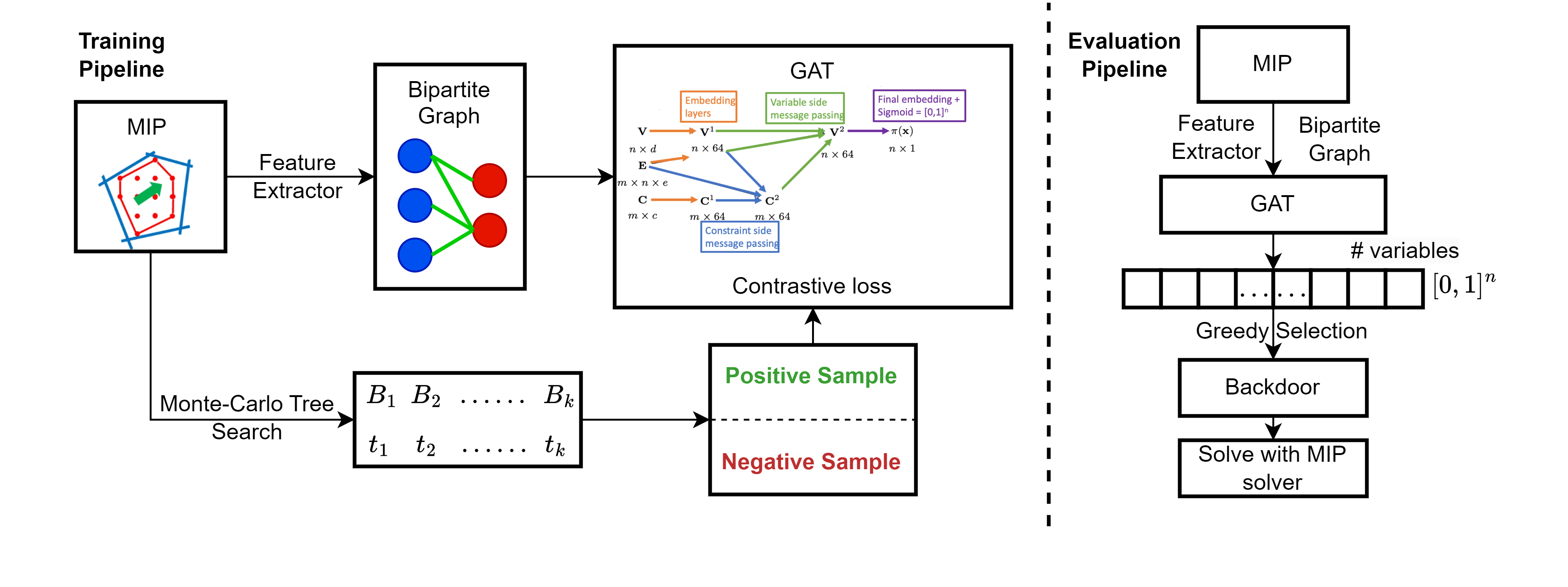
Figure 1: This figure illustrates the comprehensive training and evaluation phases for learning backdoors for MIPs with contrastive learning. In the training phase, we employ MCTS to gather backdoor samples on training instances and collect positive and negative samples. Simultaneously, a feature extractor transforms the MIP instances into a bipartite graph and collects features of the MIPs. The policy is represented by a graph attention network (GAT) and trained with a contrastive loss. In the evaluation phase, the MIP instance is converted into a bipartite graph as input for the GAT, generating a score vector as output. We greedily select variables with the highest score to obtain backdoors, which are solved using a MIP solver.

3 Contrastive Learning for Backdoor Prediction

Our goal is to learn a policy that takes as input an MIP instance and outputs a backdoor to speed up solving time. In this section, we introduce how we prepare data for contrastive learning, the policy network, and the contrastive loss used in training. Finally, we introduce how the learned policy is used in predicting backdoors. Figure 1 shows the full training and evaluation pipeline.

3.1 Data Collection

Diverging from previous approaches for finding or predicting backdoors Ferber et al. (2021); Fischetti and Monaci (2011); Dilkina et al. (2009), we incorporate contrastive learning to predict backdoors. The key challenge lies in determining high-quality positive samples and hard-to-discriminate negative samples for effective training. An MIP instance $\max\{c^{T}x\mid Ax\leq b,x_{i}\in\mathbb{Z}\,\forall i\in I\}$ can be represented as a tuple $P=(A,b,c,I)$, where $A,b,c$ are the coefficients of the constraints or objectives and $I$ is the set of integer variables. Our objective is to collect a training dataset $D$. Specifically, for every training instance $P$, we collect positive samples $S_{p}$ and negative samples $S_{n}$ specific to $P$.

We employ the Monte-Carlo Tree Search Algorithm proposed in Khalil et al. (2022) to collect candidate backdoors. MCTS will return a set of candidate backdoors with their associate tree weights in the Branch-and-Bound tree, which are approximations of the strength of backdoors. We select the top $k$ candidate backdoors $B_{1},B_{2},\dots,B_{k}$ with the highest tree weight, and solve the MIP $P$ with these candidate backdoors to obtain their runtimes $t_{1},t_{2},\dots,t_{k}$. When we solve an MIP with a backdoor, we set the branching priority for variables in the backdoor higher than other variables, i.e., we always branch on variables from the backdoor whenever there is one that needs to be branched on. Positive samples $S_{p}$ are chosen as the top $p$ backdoors with the shortest runtimes. For negative samples $S_{n}$, without additional data collection, for each positive sample in $S_{p}$, we look at the remaining candidate backdoors that are not positive samples and choose $q$ candidate backdoors with the most common variables with the positive sample backdoor. In experiments, we set $k=50$ and $p=q=5$. The approach ensure that the positive samples are backdoors with high MIP runtime performance. In contrast, the negative samples are similar to positive samples but have worse runtime performance, enabling the ML model to learn to discriminate between backdoors and non-backdoors effectively.

3.2 Data representation and Policy network

We represent the MIP $P=(A,b,c,I)$ as a bipartite graph as in  Gasse et al. (2019). The featured bipartite graph $P^{\prime}=(G,V,C,E)$, with graph $G$ containing variable nodes and constraint nodes. Additionally, there is an edge $(i,j)$ in edge matrix $\epsilon$ between a variable node $i$ and a constraint node $j$ if variable $i$ appears in constraint $j$ with nonzero coefficient, i.e., $A_{ji}\neq 0$. Constraint, variable, and edge features are represented as matrices $V\in\mathbb{R}^{n\times d},C\in\mathbb{R}^{m\times c},E\in\mathbb{R}^{m\times n\times e}$. The bipartite graph representation ensures the MIP encoding is invariant to variable and constraint permutation. Additionally, we can use a variety of predictive models designed for variable-sized graphs, enabling deployment on problems with varying numbers of variables and constraints. We use features proposed in Gasse et al. (2019), which include 15 variable features (e.g., variable types, coefficients, upper and lower bound, root LP related features), 4 constraint features (e.g., constant, sense), and 1 edge feature for coefficients.

We learn a policy $\pi$ represented by a Graph Attention Network (GAT) Brody et al. (2021), which takes the bipartite graph $P^{\prime}$ as input and outputs a score vector with one score per decision variable. To increase the modeling capacity and to manipulate node interactions proposed by our architecture, we use embedding layers in the network to first adjust the size of feature embeddings to $V^{1}\in\mathbb{R}^{n\times L},C^{1}\in\mathbb{R}^{m\times L},E^{1}\in\mathbb{R}^{|\epsilon|\times L}$ accordingly. Then, GAT performs two rounds of message passing. In the first round, each constraint node in $C^{1}$ attends to its neighbors using an attention structure with $H$ attention heads to get update constraint embeddings $C^{2}$. Similarly, each variable node in $V^{1}$ attends to its neighbors to get updated variable embeddings $V^{2}$ with another set of attention weights in the second round. Finally, the network applies a multi-layer perceptron with a sigmoid function to obtain a score between 0 and 1 for each variable. Full details of the network architecture are provided in Appendix. In experiments, $L$ and $H$ are set to 64 and 8, respectively.

Table 1: Names and the average numbers of variables, constraints, and average solve time using standard Gurobi solver (to the closest integer) of the test instances.

	Small Instances				Large Instances
Name	GISP-S	SC-S	CA-S	MIS-S	GISP-L	SC-L	CA-L	MIS-L
#Variables	988	1,000	750	1,250	1,316	1,000	1,000	1500
#Constraints	3,253	1,200	282	3,946	4,571	1,500	377	5941
Gurobi runtime	633	171	177	218	3,363	1,195	1,213	759

3.3 Training with Contrastive Loss and Applying Learned Policy

The model is trained with a contrastive loss to score each decision variable by learning to emulate superior backdoors and avoid inferior ones. Given a set of MIP instances for training, let $D=(P^{\prime},S_{p},S_{n})$ be the set of one training data where $P^{\prime}$ is the bipartite representation of MIP instance $P$, $S_{p}$ is the set of positive samples and $S_{n}$ is the set of negative samples associated with $P$. With similarity measured by dot products, we use the InfoNCE Oord et al. (2018) contrastive loss $L(P^{\prime},S_{p},S_{n})=$

$$\sum_{(P^{\prime},S_{p},S_{n})\in D}\frac{-1}{|S_{p}|}\sum_{a\in S_{p}}\log\frac{\exp(a^{T}\pi(P^{\prime})/\tau)}{\sum_{a^{\prime}\in S_{n}\cup\{a\}\exp(a^{\prime T}\pi(P^{\prime})/\tau)}}$$

to train the policy $\pi$, where $\tau$ is a temperature hyperparameter set to $0.07$ in experiment. By choosing faster solving time backdoors as positive samples and those similar to the positive ones but with lower quality as negative samples, the model learns to generate embeddings closer to positive samples and further away from negative ones.

During testing, given an MIP instance, we use the same data representation introduced in section 3.2 to convert it to a bipartite graph and use the graph as the input to GAT. Then, GAT outputs a score vector with one score for each variable. We greedily select the binary variables with the highest scores as the predicted backdoors by user-defined backdoor size. For the scorer model in Ferber et al. (2021), predicting the backdoor differs from our contrastive learning model. They first sample 50 candidate backdoors with the predefined backdoor size using the random biased sampling method Dilkina et al. (2009) and input each backdoor to the scorer model to get an output score. They select the candidate backdoor with the highest score as the predicted backdoor. The backdoor predicted by the scorer model contains strong randomness within the 50 candidate backdoors it samples, thus causing the predicted one to have highly variate performance results. Our contrastive learning model is deterministic based on greedy selection and can also output a backdoor with any size requested by the users. Finally, we assign the branching priority for variables in the backdoor before the start of the tree search in the MIP solver and then collect statistics of solving the problem to optimality for later evaluation.

Table 2: Runtime (secs) of Gurobi (grb), the scorer model (scorer), the scorer with the classifier (scorer+cls), the contrastive learning model (cl) and the contrastive learning model with the classifier (cl + cls) on GISP-S, SC-S, CA-S and MIS-S. Scorer and cl are trained on 200 instances and the classifiers are trained on another 200 instances. We report the mean, the standard deviation, 25th, 50th, and 75th percentiles, and win/tie/loss (W/T/L) counts vs. Gurobi. We report the speed improvement as a percentage inside the parentheses for the mean and median. We bold the best-performing entries.

Dataset	Solver	Mean	Std Dev	25 pct	Median	75 pct	W/T/L vs grb
GISP-S	grb	633	154	513	615	731	-
	scorer	544 (14.1%)	117	453	543 (11.7%)	611	74/0/26
	scorer + cls	578 (8.7%)	128	502	586 (4.7%)	637	43/32/25
	cl	533 (15.8%)	120	441	524 (14.8%)	612	84/0/16
	cl + cls	560 (11.5%)	135	462	555 (9.8%)	653	59/27/14
SC-S	grb	171	189	50.8	101	216	-
	scorer	244 (-42.69%)	219	67.2	148 (-46.5%)	295	27/0/73
	scorer + cls	203 (-18.7%)	195	62.1	142 (-40.6%)	256	15/57/28
	cl	149 (12.9%)	163	42.5	79.8 (20.1%)	195	77/0/23
	cl + cls	153 (10.5%)	165	49.4	79.4 (21.4%)	197	52/27/21
CA-S	grb	177	94.6	110	151	229	-
	scorer	224 (-26.6%)	120	125	217 (-43.7%)	293	17/0/83
	scorer + cls	194 (-9.6%)	112	119	191 (-26.5%)	243	14/52/34
	cl	156 (11.9%)	83.0	88.5	146 (3.3%)	195	68/0/32
	cl + cls	170 (4.0%)	96.2	103	139 (7.94%)	227	46/28/26
MIS-S	grb	218	231	79.7	147	267	-
	scorer	236 (-8.3%)	258	89.9	156 (-6.1%)	269	36/0/64
	scorer + cls	219 (-0.5%)	237	82.3	154 (-4.8%)	264	24/46/30
	cl	184 (15.6%)	179	76.8	127 (13.6%)	214	69/0/31
	cl + cls	190 (12.8%)	197	80.2	136 (7.5%)	227	44/35/21

4 Empirical Evaluation

In this section, we introduce problem domains and instance sizes for evaluation. We explain the experiment setup, including data collection, baselines, metrics, and hyperparameters, and then present the results. Our code will be made available to the public upon publication.

4.1 Problem Domains and Instance Generation

We evaluate on four NP-hard problem domains, Generalized Independent Set Problem (GISP), Set Cover (SC), Combinatorial Auction (CA), and Maximum Independent Set (MIS), that are widely used in existing studies Song et al. (2020); Ferber et al. (2021); Huang et al. (2023). For each problem domain, we generate Small (S) and Large (L) instances for it. Following Ferber et al. (2021), GISP-S and GISP-L instances are generated with 150 nodes and 175 nodes, respectively, with the node reward set to 100 and edge removal cost set to 1; In order to keep a similar evaluation procedure (e.g., Gurobi being able to solve to optimality within certain runtime) and diverse hardness of the problems, we choose the size of the three other problem domains as follows: Following Huang et al. (2023), SC-S instances have 1,000 variables and 1,200 constraints and SC-L instances have 1,000 variables and 1,500 constraints, with density set to 0.05 for both; Following  Leyton-Brown et al. (2000), CA-S instances are generated with 150 items and 750 bids and CA-L instances are generated with 200 items and 1,000 bids according to the arbitrary relations; Following Huang et al. (2023), MIS-S and MIS-L instances are generated according to the Erdos-Renyi random graph model Erdős et al. (1960), with an average degree of 4 and 1,250 and 1,500 nodes, respectively. Previous work Ferber et al. (2021) evaluates on other problem domains, such as Neural Network Verification and Facility Location. We are not able to collect backdoor data with MCTS on these two problem domains and evaluate them since they contain non-binary variables, and MCTS backdoor collection in Khalil et al. (2022) currently only works with mixed-binary instances, i.e., instances with no general integer variables, due to the ease of implementation of the tree weight for binary problems. In practice, we can still use randomly sampled backdoors for training and the rest of the pipeline remains the same. For each test set, Table 1 shows its average numbers of variables and constraints and average solve time using a standard Gurobi solver. More details of instance generation are included in the Appendix.

4.2 Experiment Setup

For data collection, we generate 200 small instances for each problem domain. We use the MCTS framework to collect backdoors of size 8 for each instance over 5 hours with 10 parallel workers. We follow Khalil et al. (2022) and choose 8, which shows promising results on finding high-quality backdoors on 164 problem domains From MIPLIB2017. We select the top 50 backdoors measured by tree weight function, solve the problems using those backdoors with MIP solver, and record the runtimes. For contrastive loss, we select the first 5 fastest backdoors as positive samples and used the methods in section 3.1 without additional data collection to select 5 negative samples per each positive one.

We compare our contrastive learning model (cl) with several baselines: Gurobi (grb), the scorer model (scorer) and the scorer with the classifier (scorer+cls). scorer is the previous method  Ferber et al. (2021) that predicts the score for candidate backdoors using supervised learning and scorer+cls is scorer with cls to predict whether to use the backdoor output by the score or not. The scorer and cl models are trained with 200 instances, with 160 and 40 instances for training and validation, respectively. For cls, we generate another 200 instances, with 160 and 40 instances for training and validation, respectively. To train the classifier for scorer+cls, we use random sampling based on the LP relaxation Dilkina et al. (2009) to generate random 50 candidate backdoors and use scorer to select the best one to collect runtime statistics. Then, we assign labels for each instance based on the runtime of the selected backdoor over the Gurobi runtime and use a cross-entropy loss to train the classifier following Ferber et al. (2021). To train the classifier for cl+cls, we collect the runtime statistics from the backdoor output directly from cl model and the rest is the same as cl+cls.

To compare the performance of the methods, we test on 100 instances for each problem domain and report summary statistics of runtime to solve the problem to optimality, including mean, standard deviation, 25th percentile, median, and 75th percentile. We also report the wins, ties, and losses over Gurobi. We consider the runtime of the full pipeline, including feature extractor, inference for the GAT model, sampling or greedy selection, and solving the MIP. When cls suggests using Gurobi, we record a “tie” to give insight into model predictions even though there is a slight loss in runtime due to the ML overhead.

We solve MIPs with single-threaded Gurobi 10.0 on four 64-core machines with Intel 2.1GHz CPUs and 264GB of memory. Training is done on an NVIDIA Tesla V100 GPU with 112GB memory. For cl model, we use the Adam optimizer Kingma and Ba (2014) with a learning rate of $5\times 10^{-4}$ and a weight decay of 0.01. We use a batch size of 32 and train for 100 epochs. For scorer and cls, the learning rate is set to $5\times 10^{-3}$ and a batch size of 128 and train for 100 epochs. Due to the fact of pairwise ranking loss in the scorer, the training for scorer is extremely expensive, which takes around 10-15 hours, while the training time for cl model is less than 30 minutes. The more efficient use of training data significantly improves our cl model.

(a) GISP-L

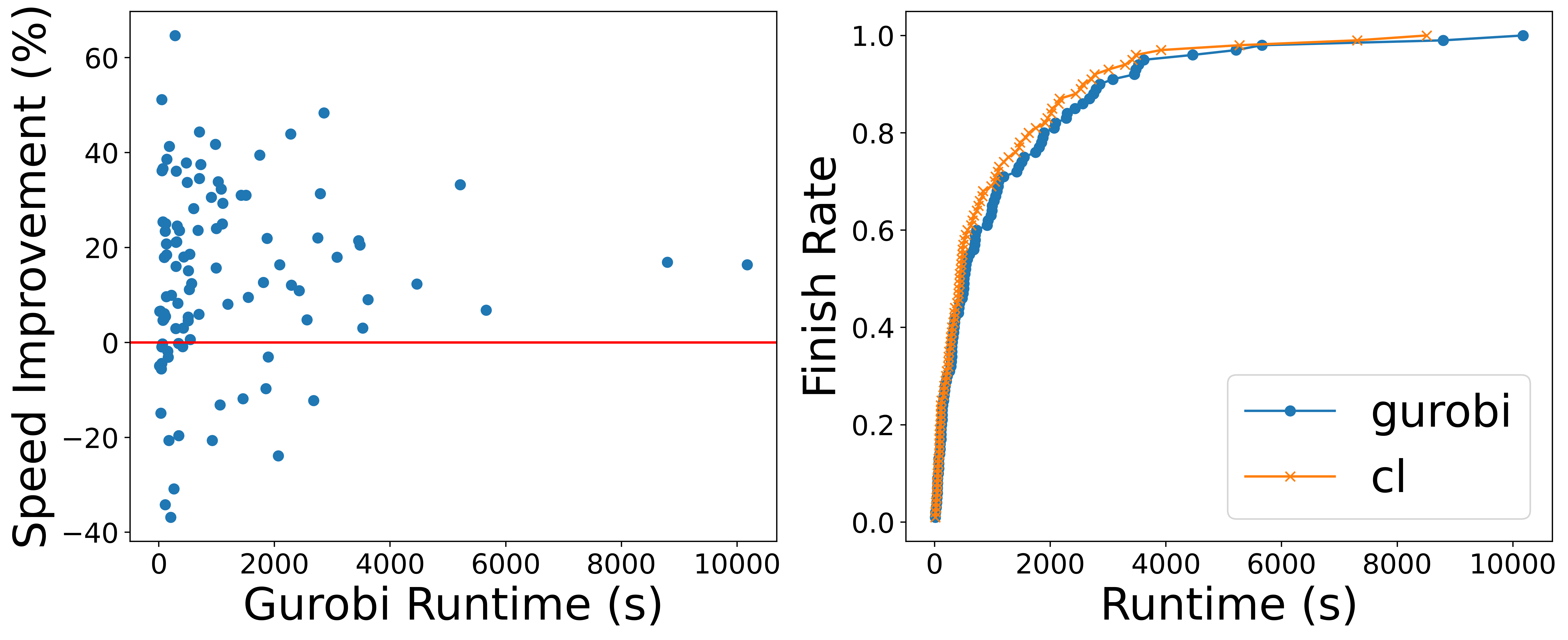
(b) SC-L

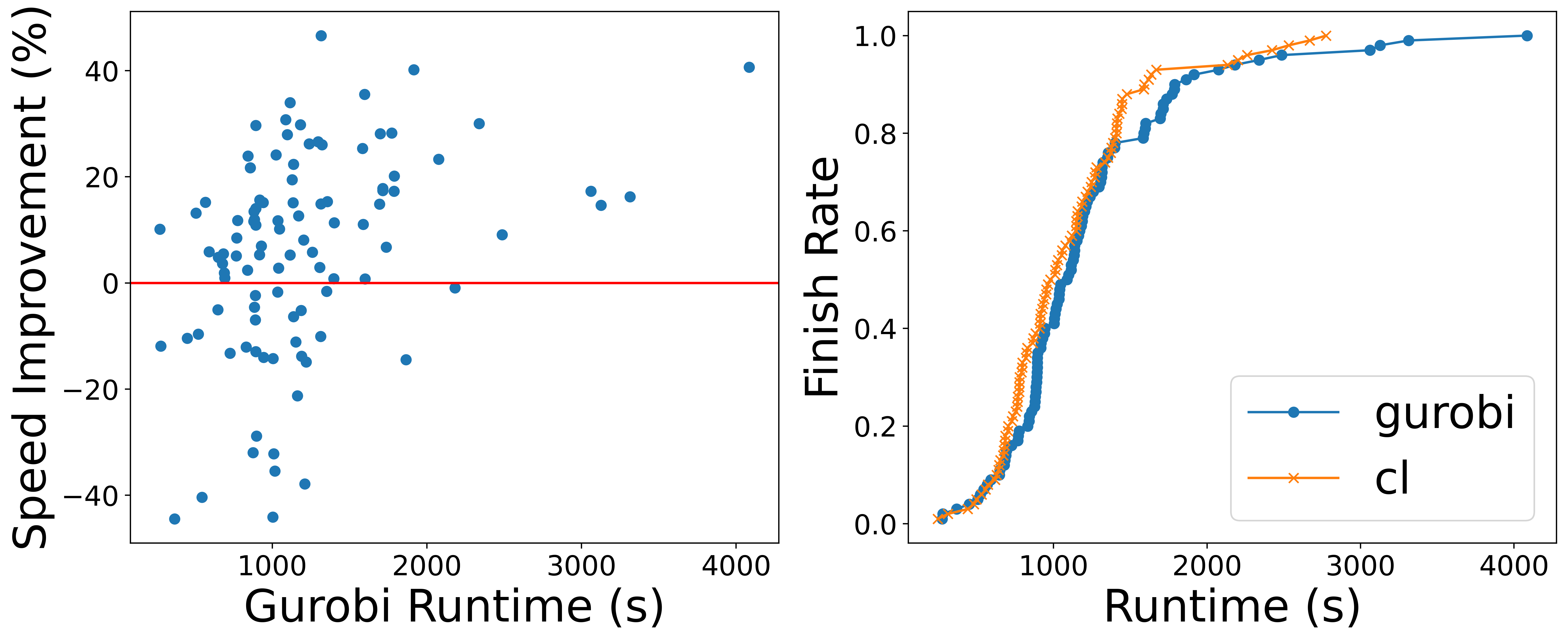
(c) CA-L

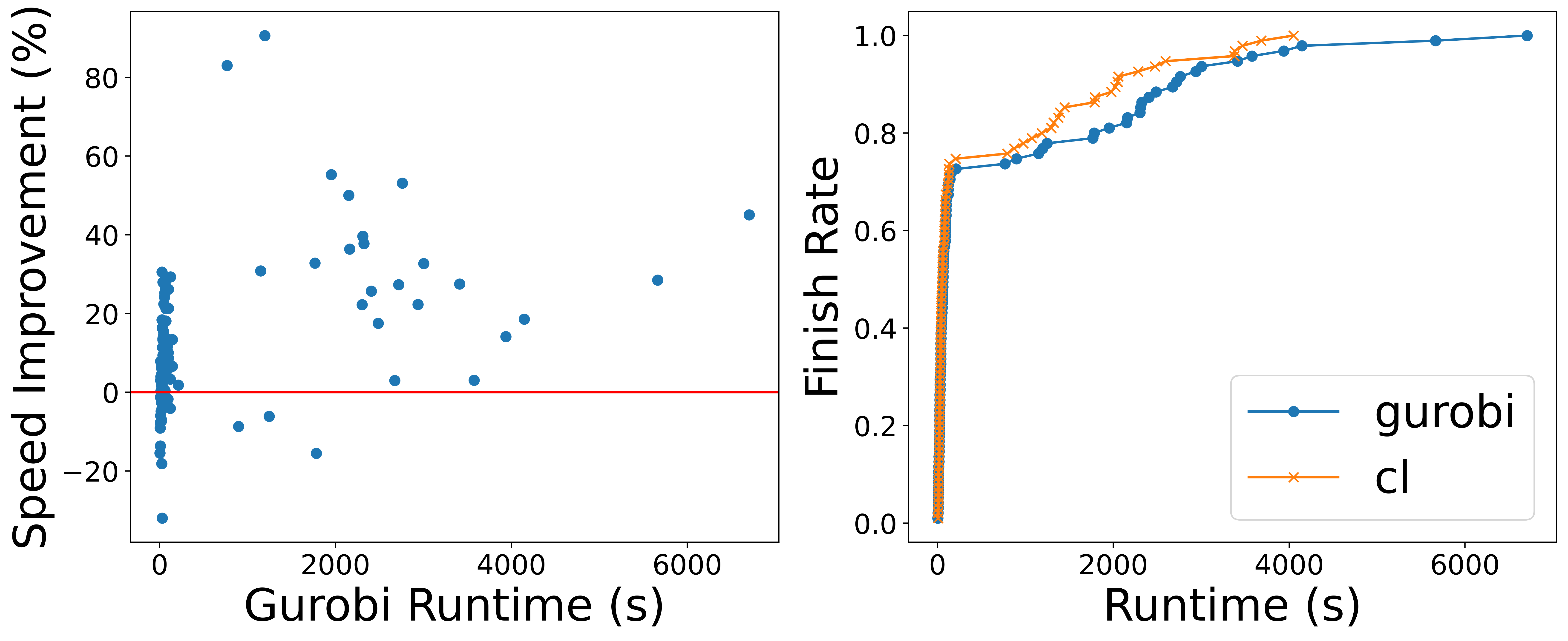
(d) MIS-L

Figure 2: This figure shows the runtime of Gurobi (grb) and contrastive learning model (cl) on GISP-L, SC-L, CA-L, and MIS-L through two different types of plots. The left part is a scatter plot with Gurobi runtime as the x-axis and the speed improvement as the percentage of cl over grb as the y-axis. The points above the red line are ones where cl is better than grb and vice versa. The right part shows the finish rate as a function of runtime. The finish rate for a given runtime is the fraction of instances solved to optimality within the runtime. The blue line is grb and the orange line is cl, with every dot indicating one finished instance. The figures show that cl outperforms grb on average and specifically provides speedups on the harder instances in each distribution.

Table 3: Evaluating generalization to larger problem size: Runtime (secs) of standard Gurobi (grb) and the contrastive learning model (cl) on GISP-L, SC-L, CA-L, MIS-L. The model is trained on 200 small instances for each problem domain. We report the mean, the standard deviation, 25th, 50th, and 75th percentiles, and win/tie/loss (W/T/L) counts vs. Gurobi. We report the speed improvement as a percentage inside the parentheses for the mean and median. We bold the best-performing entries.

Dataset	Solver	Mean	Std Dev	25 pct	Median	75 pct	W/L vs grb
GISP-L	grb	3,363	989	2,611	3,303	4,049	-
	cl	2,879 (14.4%)	785	2,288	2,910 (11.9%)	3,331	77/23
SC-L	grb	1,195	1,692	161	519	1,597	-
	cl	1,003 (16.1%)	1,433	143	435 (16.0%)	1,309	78/22
CA-L	grb	1,213	625	881	1,093	1,353	-
	cl	1,096 (9.6%)	487	767	994 (9.1%)	1,159	69/31
MIS-L	grb	759	1,356	128	263	1,023	-
	cl	550 (27.5%)	987	127	256 (2.7%)	501	75/25

We conduct the following sets of experiments:

• We compare cl and cl+cls against grb, scorer, scorer+cls on the small instances;

• We test the generalizability of the cl model (trained on the small instances) on the large instances and compare it against grb.

• Ablation study: For GISP-S, SC-S, we test how contrastive learning and MCTS data collection separately affect the performance of backdoor predicting.

Table 4: Evaluating the role of the backdoor collection strategy: Runtime (secs) of standard Gurobi (grb), the scorer model (scorer), and the contrastive learning model (cl) with different backdoor collection methods, MCTS, and sampling. We report the mean, the standard deviation, 25th, 50th, and 75th percentiles, and win/tie/loss (W/T/L) counts vs. Gurobi. We bold the best-performing entries.

Dataset	Solver	Mean	Std Dev	25 pct	Median	75 pct	W/L vs grb
GISP-S	scorer + Sampling	601	152	518	580	681	49/51
	scorer + MCTS	544	117	453	543	611	74/26
	cl + Sampling	565	132	455	556	634	67/33
	cl + MCTS	533	120	441	524	612	84/16
SC-S	scorer + Sampling	287	358	85.4	167	359	3/97
	scorer + MCTS	244	219	67.2	148	295	27/73
	cl + Sampling	186	196	48.5	107	254	43/57
	cl + MCTS	149	163	42.5	79.8	195	77/23

4.3 Results

From the backdoor collection for all the problem domains, we observe significant improvement in MCTS data collection over the previous sampling method. For the 50 backdoors on each of the 200 instances, we collect the summary statistic of 10,000 backdoors on how many backdoors have a faster runtime over standard Gurobi. The model aims to learn to predict the best backdoor, so we also collect how many instances have the best backdoor among 50 backdoors that can beat standard Gurobi. For GISP-S, the backdoor collection exhibits superior quality, with 7,269 out of 10,000 backdoors outperforming Gurobi and all 200 instances having at least one of them. For SC-S, 3,933 out of 10,000 backdoors outperform Gurobi in 169 of 200 instances having at least one of them. However, CA-S faces the challenge of having low backdoor quality, with only 850 out of 10,000 backdoors outperforming Gurobi in 94 out of 200 instances. For MIS-S, 2,527 out of 10,000 backdoors are faster than Gurobi in 124 out of 200 instances. The histograms of backdoor collection quality are included in the Appendix. In contrast,  Ferber et al. (2021) collected data on SC, CA, and MIS but found the best-sampled backdoors under Perform Gurobi on all instances. With our MCTS data collection, on these three problem domains, we have at least 47% of instances with at least one backdoor that can outperform Gurobi, and for SC, we can even reach around 85%. Also, the performance of scorer is highly related to the quality of sampled candidate backdoors, if the best-sampled ones under-performed Gurobi during data collection, then no matter how accurate their models, they could never outperform standard Gurobi during evaluation. But for cl, even when the sampling does not yield a backdoor that outperforms Gurobi during data collection, our greedy selection approach may still be able to output a better-performance backdoor at test time. With the MCTS backdoor collection and cl model, we can find high-quality backdoors on more problem domains and apply ML to predict backdoors for them.

We present results on 100 small test instances in Table 2. cl consistently performs better than scorer and has more than 10% improvement on the average runtime in all problem domains, even in those where the scorer does not work. scorer performs well on GISP-S with 14.1% speed improvement, but perform worse than grb on SC-S, CA-S, MIS-S with 67.8%, 26.6%, 8.3% increase on the average runtime. The reason is for GISP, the problem formulation as MIP has good quality in that only the first 150 variables have LP-relaxation values, not 0 or 1 in all instances, but for other problem domains, the 0 or 1 value in LP-relaxation is more varied and does not have a specific pattern. The probability of randomly generating a good backdoor of size 8 from a set of around 1,000 variables would be super hard, so there is a high chance that the 50 candidate backdoors do not contain any good backdoor. Even scorer has high accuracy, using scorer would still yield a worse performance than Gurobi. However, in cl, we benefit from greedy selection, and as the experiment results show, the backdoor output by cl has high quality, leading to 77, 68, 69 wins over Gurobi on SC-S, CA-S, and MIS-S, respectively. For cls, it only improves the runtime when scorer performs very badly, and when the model performs well, it will categorize more wins to tie than more losses to tie. cls is not a good fit for cl and it requires additional MIP instances and training data collection. Consider in a real-world problem domain where we have a limited number of instances, using all the data to train cl would be a better and more elegant method.

To show the generalizability of cl, we test cl trained on 100 small instances on 100 large instances of the same problem. This experiment shows that when the instances are large and MCTS becomes too slow to collect data, we can still use cl trained on smaller instances. As the results shown in Table 3, cl still consistently outperforms grb. On GISP-L and CA-L, cl achieves only a slight percentage drop on mean over grb compared to the small instances; On SC-L and MIS-L even achieve better performance. The results show that cl also performs well on larger and harder instances, as illustrated by Figure 2. The figure compares the runtime of grb and cl in terms of speed improvement and finish rate. On the left part, the dots under the red line are mostly easy instances, and our model almost gains 100% win for the hard instances. On the right side, the orange line is consistently above the blue line, except for the starting line, which is an easy instance. The results clearly show cl has great generalizability to the problem with the same domain and opens the potential for learning backdoors on much larger real-world problem domains. The same set of figures on small instances is included in the Appendix.

For the ablation study, we evaluate how contrastive learning and the MCTS backdoor collection contribute to the model performance. We collect another set of backdoor data on the same instances using biased random sampling, the backdoor collection method used by Ferber et al. (2021). We compare the performance of scorer + sampling, scorer + MCTS, cl + sampling, and cl + MCTS on GISP-S and SC-S and Table 4 reports the runtime statistics. The result shows there is an improvement in performance for both scorer and cl when using MCTS, showing the benefit of replacing random sampling with MCTS for data collection. The results also show that the cl consistently performs better than the scorer with the same data collection method, showing the benefit of contrastive learning over the previous learning-to-rank method. Overall, cl + MCTS has the best performance on GISP-S and SC-S.

5 Conclusion

This paper introduces a contrastive learning framework to predict effective backdoors for MIPs. We utilize a Monte-Carlo tree search method to collect training data of better quality than previous methods. Empirical results on several common problem domains indicated that the contrastive learning model significantly outperforms existing baselines. It also achieved good generalization performance on larger-size instances. Beyond finding better backdoors, our model requires less time and resources for training and reduces randomness compared to the previous scorer model. For future work, we want to develop some theory related to backdoors to understand the theoretical properties of backdoors. Moreover, given the recent successes of contrastive learning, it can be applied to other MIP learning problems, potentially becoming a foundational method for ML in combinatorial optimization.

References

- Balas and Ho [1980] Egon Balas and Andrew Ho. Set covering algorithms using cutting planes, heuristics, and subgradient optimization: a computational study. In Combinatorial Optimization, pages 37–60. Springer, 1980.
- Brody et al. [2021] Shaked Brody, Uri Alon, and Eran Yahav. How attentive are graph attention networks? arXiv preprint arXiv:2105.14491, 2021.
- Chen et al. [2020] Ting Chen, Simon Kornblith, Mohammad Norouzi, and Geoffrey Hinton. A simple framework for contrastive learning of visual representations. In International conference on machine learning, pages 1597–1607. PMLR, 2020.
- Chmiela et al. [2021] Antonia Chmiela, Elias Khalil, Ambros Gleixner, Andrea Lodi, and Sebastian Pokutta. Learning to schedule heuristics in branch and bound. Advances in Neural Information Processing Systems, 34:24235–24246, 2021.
- Dilkina et al. [2009] Bistra Dilkina, Carla P Gomes, and Ashish Sabharwal. Backdoors in the context of learning. In International Conference on Theory and Applications of Satisfiability Testing, pages 73–79. Springer, 2009.
- Duan et al. [2022] Haonan Duan, Pashootan Vaezipoor, Max B Paulus, Yangjun Ruan, and Chris Maddison. Augment with care: Contrastive learning for combinatorial problems. In International Conference on Machine Learning, pages 5627–5642. PMLR, 2022.
- Erdős et al. [1960] Paul Erdős, Alfréd Rényi, et al. On the evolution of random graphs. Publ. math. inst. hung. acad. sci, 5(1):17–60, 1960.
- Ferber et al. [2021] Aaron Ferber, Jialin Song, Bistra Dilkina, and Yisong Yue. Learning pseudo-backdoors for mixed integer programs, 2021.
- Fischetti and Monaci [2011] Matteo Fischetti and Michele Monaci. Backdoor branching. In International Conference on Integer Programming and Combinatorial Optimization, pages 183–191. Springer, 2011.
- Floudas and Lin [2005] Christodoulos A Floudas and Xiaoxia Lin. Mixed integer linear programming in process scheduling: Modeling, algorithms, and applications. Annals of Operations Research, 139:131–162, 2005.
- Gasse et al. [2019] Maxime Gasse, Didier Chételat, Nicola Ferroni, Laurent Charlin, and Andrea Lodi. Exact combinatorial optimization with graph convolutional neural networks. Advances in neural information processing systems, 32, 2019.
- Gavish and Pirkul [1991] Bezalel Gavish and Hasan Pirkul. Algorithms for the multi-resource generalized assignment problem. Management science, 37(6):695–713, 1991.
- Gupta et al. [2020] Prateek Gupta, Maxime Gasse, Elias Khalil, Pawan Mudigonda, Andrea Lodi, and Yoshua Bengio. Hybrid models for learning to branch. Advances in neural information processing systems, 33:18087–18097, 2020.
- Gurobi Optimization, LLC [2023] Gurobi Optimization, LLC. Gurobi Optimizer Reference Manual, 2023.
- Han et al. [2022] Qingyu Han, Linxin Yang, Qian Chen, et al. A gnn-guided predict-and-search framework for mixed-integer linear programming. In ICLR, 2022.
- He et al. [2014] He He, Hal Daume III, and Jason M Eisner. Learning to search in branch and bound algorithms. Advances in neural information processing systems, 27, 2014.
- Hjelm et al. [2018] R Devon Hjelm, Alex Fedorov, Samuel Lavoie-Marchildon, Karan Grewal, Phil Bachman, Adam Trischler, and Yoshua Bengio. Learning deep representations by mutual information estimation and maximization. arXiv preprint arXiv:1808.06670, 2018.
- Hochbaum and Pathria [1997] Dorit S Hochbaum and Anu Pathria. Forest harvesting and minimum cuts: a new approach to handling spatial constraints. Forest Science, 43(4):544–554, 1997.
- Huang et al. [2023] Taoan Huang, Aaron M Ferber, Yuandong Tian, Bistra Dilkina, and Benoit Steiner. Searching large neighborhoods for integer linear programs with contrastive learning. In International Conference on Machine Learning, pages 13869–13890. PMLR, 2023.
- Jaiswal et al. [2020] Ashish Jaiswal, Ashwin Ramesh Babu, Mohammad Zaki Zadeh, Debapriya Banerjee, and Fillia Makedon. A survey on contrastive self-supervised learning. Technologies, 9(1):2, 2020.
- Khalil et al. [2016] Elias Khalil, Pierre Le Bodic, Le Song, George Nemhauser, and Bistra Dilkina. Learning to branch in mixed integer programming. In Proceedings of the AAAI Conference on Artificial Intelligence, volume 30, 2016.
- Khalil et al. [2017] Elias B Khalil, Bistra Dilkina, George L Nemhauser, Shabbir Ahmed, and Yufen Shao. Learning to run heuristics in tree search. In Ijcai, pages 659–666, 2017.
- Khalil et al. [2022] Elias B Khalil, Pashootan Vaezipoor, and Bistra Dilkina. Finding backdoors to integer programs: a monte carlo tree search framework. In Proceedings of the AAAI Conference on Artificial Intelligence, volume 36, pages 3786–3795, 2022.
- Khosla et al. [2020] Prannay Khosla, Piotr Teterwak, Chen Wang, Aaron Sarna, Yonglong Tian, Phillip Isola, Aaron Maschinot, Ce Liu, and Dilip Krishnan. Supervised contrastive learning. Advances in neural information processing systems, 33:18661–18673, 2020.
- Kingma and Ba [2014] Diederik P Kingma and Jimmy Ba. Adam: A method for stochastic optimization. arXiv preprint arXiv:1412.6980, 2014.
- Kottler et al. [2008] Stephan Kottler, Michael Kaufmann, and Carsten Sinz. Computation of renameable horn backdoors. In Theory and Applications of Satisfiability Testing–SAT 2008: 11th International Conference, SAT 2008, Guangzhou, China, May 12-15, 2008. Proceedings 11, pages 154–160. Springer, 2008.
- Labassi et al. [2022] Abdel Ghani Labassi, Didier Chételat, and Andrea Lodi. Learning to compare nodes in branch and bound with graph neural networks. Advances in Neural Information Processing Systems, 35:32000–32010, 2022.
- Land and Doig [2010] Ailsa H Land and Alison G Doig. An automatic method for solving discrete programming problems. Springer, 2010.
- Leyton-Brown et al. [2000] Kevin Leyton-Brown, Mark Pearson, and Yoav Shoham. Towards a universal test suite for combinatorial auction algorithms. In Proceedings of the 2nd ACM conference on Electronic commerce, pages 66–76, 2000.
- Logeswaran and Lee [2018] Lajanugen Logeswaran and Honglak Lee. An efficient framework for learning sentence representations. arXiv preprint arXiv:1803.02893, 2018.
- Mulamba et al. [2020] Maxime Mulamba, Jayanta Mandi, Michelangelo Diligenti, Michele Lombardi, Victor Bucarey, and Tias Guns. Contrastive losses and solution caching for predict-and-optimize. arXiv preprint arXiv:2011.05354, 2020.
- Nair et al. [2020] Vinod Nair, Sergey Bartunov, Felix Gimeno, et al. Solving mixed integer programs using neural networks. arXiv preprint arXiv:2012.13349, 2020.
- Oord et al. [2018] Aaron van den Oord, Yazhe Li, and Oriol Vinyals. Representation learning with contrastive predictive coding. arXiv preprint arXiv:1807.03748, 2018.
- Paris et al. [2006] Lionel Paris, Richard Ostrowski, Pierre Siegel, and Lakhdar Sais. Computing horn strong backdoor sets thanks to local search. In 2006 18th IEEE International Conference on Tools with Artificial Intelligence (ICTAI’06), pages 139–143. IEEE, 2006.
- Paulus et al. [2022] Max B Paulus, Giulia Zarpellon, Andreas Krause, Laurent Charlin, and Chris Maddison. Learning to cut by looking ahead: Cutting plane selection via imitation learning. In International conference on machine learning, pages 17584–17600. PMLR, 2022.
- Pohl [1970] Ira Pohl. Heuristic search viewed as path finding in a graph. Artificial intelligence, 1(3-4):193–204, 1970.
- Song et al. [2018] Jialin Song, Ravi Lanka, Albert Zhao, Aadyot Bhatnagar, Yisong Yue, and Masahiro Ono. Learning to search via retrospective imitation. arXiv preprint arXiv:1804.00846, 2018.
- Song et al. [2020] Jialin Song, Yisong Yue, Bistra Dilkina, et al. A general large neighborhood search framework for solving integer linear programs. Advances in Neural Information Processing Systems, 33:20012–20023, 2020.
- Sonnerat et al. [2021] Nicolas Sonnerat, Pengming Wang, Ira Ktena, Sergey Bartunov, and Vinod Nair. Learning a large neighborhood search algorithm for mixed integer programs. arXiv preprint arXiv:2107.10201, 2021.
- Tang et al. [2020] Yunhao Tang, Shipra Agrawal, and Yuri Faenza. Reinforcement learning for integer programming: Learning to cut. In International conference on machine learning, pages 9367–9376. PMLR, 2020.
- Tarjan and Trojanowski [1977] Robert Endre Tarjan and Anthony E Trojanowski. Finding a maximum independent set. SIAM Journal on Computing, 6(3):537–546, 1977.
- Tong et al. [2021] Zekun Tong, Yuxuan Liang, Henghui Ding, Yongxing Dai, Xinke Li, and Changhu Wang. Directed graph contrastive learning. Advances in neural information processing systems, 34:19580–19593, 2021.
- Toth and Vigo [2002] Paolo Toth and Daniele Vigo. The vehicle routing problem. SIAM, 2002.
- Veličković et al. [2017] Petar Veličković, Guillem Cucurull, Arantxa Casanova, Adriana Romero, Pietro Lio, and Yoshua Bengio. Graph attention networks. arXiv preprint arXiv:1710.10903, 2017.
- Williams et al. [2003] Ryan Williams, Carla P Gomes, and Bart Selman. Backdoors to typical case complexity. In IJCAI, volume 3, pages 1173–1178, 2003.
- You et al. [2020] Yuning You, Tianlong Chen, Yongduo Sui, Ting Chen, Zhangyang Wang, and Yang Shen. Graph contrastive learning with augmentations. Advances in neural information processing systems, 33:5812–5823, 2020.
- Zhang et al. [2023] Jiayi Zhang, Chang Liu, Xijun Li, Hui-Ling Zhen, Mingxuan Yuan, Yawen Li, and Junchi Yan. A survey for solving mixed integer programming via machine learning. Neurocomputing, 519:205–217, 2023.