Learning to Robustly Reconstruct Dynamic Scenes from Low-light Spike Streams

Abstract

As a neuromorphic sensor with high temporal resolution, spike camera can generate continuous binary spike streams to capture per-pixel light intensity. We can use reconstruction methods to restore scene details in high-speed scenarios. However, due to limited information in spike streams, low-light scenes are difficult to effectively reconstruct. In this paper, we propose a bidirectional recurrent-based reconstruction framework, including a Light-Robust Representation (LR-Rep) and a fusion module, to better handle such extreme conditions. LR-Rep is designed to aggregate temporal information in spike streams, and a fusion module is utilized to extract temporal features. Additionally, we have developed a reconstruction benchmark for high-speed low-light scenes. Light sources in the scenes are carefully aligned to real-world conditions. Experimental results demonstrate the superiority of our method, which also generalizes well to real spike streams. Related codes and proposed datasets will be released after publication.

1 Introduction

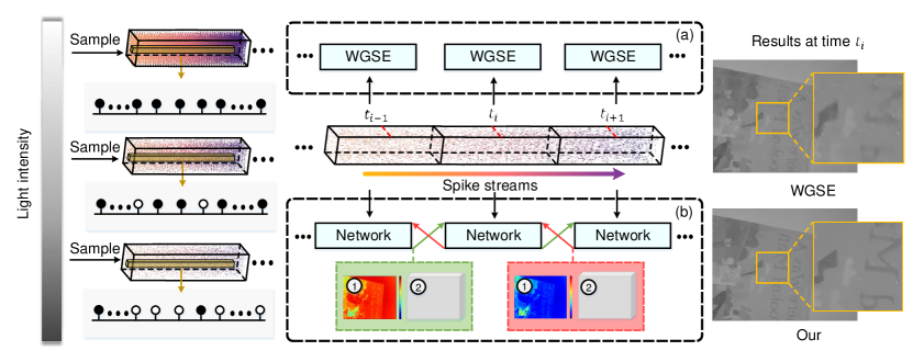
Figure 1: Overview of reconstruction for high-speed spike streams. Left: with decreasing light intensity, more sparse spike streams are difficult to extract features. A black circle is a spike. Middle: (a) The state-of-the-art method, WGSE [24]. The arrow with a gradient color is the timeline. (b) Our reconstruction method. Green (red) lines denote the forward (backward) data flow. ① (②) is the release time of spikes (temporal features). ① (②) in forward and backward data flow is independent. Right: reconstructed results from WGSE and our method.

As a neuromorphic sensor with high temporal resolution (40000 Hz), spike camera [31, 8] has shown enormous potential for high-speed visual tasks, such as reconstruction [26, 32, 30, 27, 33, 2], optical flow estimation [7, 29, 23], and depth estimation [25, 16, 14]. Different from event cameras [15, 3, 1], it can record per-pixel light intensity by accumulating photons and firing continuous binary spike streams. Correspondingly, high-speed dynamic scenes can be reconstructed from spike streams. Recently, many deep learning methods have advanced this field and shown great success in reconstructing more detailed scenes. However, existing methods struggle to perform well in low-light environments due to insufficient information in spike streams.

A dilemma arises for visual sensors, that is, the quality of sampled data can greatly decrease in a low-light environment [6, 12, 11, 29, 5]. Low-quality data creates many difficulties for all kinds of vision tasks. Similarly, the reconstruction for the spike camera also suffers from this problem. To improve the performance of reconstruction in low-light high-speed scenes, two non-trivial matters should be carefully considered. First, Constructing a low-light high-speed scene benchmark for spike camera is crucial to evaluating different methods. However, due to the frame rate limitations of traditional cameras, it is difficult to capture images clearly in real high-speed scenes as supervised signals. Instead of it, a reasonable way is to synthesize datasets for spike camera [27, 33, 7, 25]. To ensure the reliability of the reconstruction benchmark, synthetic low-light high-speed scenes should be as consistent as possible with the real world, e.g., light source. Second, as shown in Fig. 1, with the decrease of illuminance in the environment, the total number of spikes in spike streams decreases greatly which means the valid information in spike streams can greatly decrease. Fig. 1(a) shows that previous methods often fail under low-light conditions since they have no choice but to rely on inadequate information.

In this work, we aim to address all two issues above-mentioned. In more detail, a reconstruction benchmark for high-speed low-light scenes is proposed. We carefully design the scene by controlling the type and power of the light source and generating noisy spike streams based on [28]. Besides, we propose a light-robust reconstruction method as shown in Fig. 1(b). Specifically, to compensate for information deficiencies in low-light spike streams, we propose a light-robust representation (LR-Rep). In LR-Rep, the release time of forward and backward spikes is used to update a global inter-spike interval (GISI). Then, to further excavate temporal information in spike streams, LR-Rep is fused with forward (backward) temporal features. During the feature fusion process, we add alignment information to avoid the misalignment of motion from different timestamps. Finally, the scene is clearly reconstructed from fused features.

Empirically, we show the superiority of our reconstruction method. Importantly, our method also generalizes well to real spike streams. In addition, extensive ablation studies demonstrate the effectiveness of each component. The main contributions of this paper can be summarized as follows:

$\bullet$ A reconstruction benchmark for high-speed low-light scenes is proposed. We carefully construct varied low-light scenes that are close to reality.

$\bullet$ We propose a bidirectional recurrent-based reconstruction framework where a light-robust representation, LR-Rep, and fusion module can effectively compensate for information deficiencies in low-light spike streams.

$\bullet$ Experimental results on real and synthetic datasets have shown our method can more effectively handle spike streams under different light conditions than previous methods.

2 Related Work

2.1 Low-light Vision

Low-light environment has always been a challenge not only for human perception but also for computer vision methods. For traditional cameras, some works concern the enhancement of low-light images. [20] propose the LOL dataset containing low/normal-light image pairs and propose a deep Retinex-Net including a Decom-Net for decomposition and an Enhance-Net for illumination adjustment. [9] proposes the EnlightenGAN which is first trained on unpaired data to low-light image enhancement. [6] proposes Zero-DCE which formulates light enhancement as a task of image-specific curve estimation with a deep network. Besides, some work focuses on the robustness of vision task to low-light, e.g., object detection. [17] proposes a method of domain adaptation for merging multiple models to handle objects in a low-light situation. [13] integrates a new non-local feature aggregation method and a knowledge distillation technique to with the detector networks. [18] combines with the image enhancement algorithm to improves the accuracy of object detection. For spike camera, it are also affected by low-light environments. [4] propose a real low-light high-speed dataset for reconstruction. However, it lacks corresponding image sequences as ground truth. To solve the challenge in the reconstruction of low-light spike streams, We have fully developed the task including a reconstruction benchmark for high-speed low-light scenes and a light-robust reconstruction method.

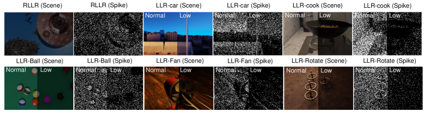
Figure 2: Proposed datasets, RLLR and LLR. RLLR includes the random scenes and LLR includes carefully designed scenes.

2.2 Reconstruction for Spike Camera

The reconstruction of high-speed dynamic scenes has been a popular topic for spike camera. Based on the statistical characteristics of spike stream, [31] first reconstruct high-speed scenes. [26] improved the smoothness of reconstructed scenes by introducing motion aligned filter. [32] construct a dynamic neuron extraction model to distinguish the dynamic and static scenes. For enhancing reconstruction results, [30] uses short-term plasticity mechanism to exact motion area. [27] first proposes a deep learning-based reconstruction framework, Spk2ImgNet (S2I), to handle the challenges brought by both noise and high-speed motion. [2] build a self-supervised reconstruction framework by introducing blind-spot networks. It achieves desirable results compared with S2I. The reconstruction method [24] presents a novel Wavelet Guided Spike Enhancing (WGSE) paradigm. By using multi level wavelet transform, the noise in the reconstructed results can be effectively suppressed.

2.3 Spike Camera Simulation

Spike camera simulation is a popular way to generate spike streams and accurate labels. [27] first convert interpolated image sequences with high frame rate into spike stream. Based on [27], [33, 10, 28] add some random noise to generate spike streams more accurately. To avoid motion artifacts caused by interpolation, [7] presents the spike camera simulator (SPCS) combining simulation function and rendering engine tightly. Then, based on SPCS, optical flow datasets for spike camera are first proposed. [25] generate the first spike-based depth dataset by the spike camera simulation.

3 Reconstruction Datasets

In order to train and evaluate the performance of reconstruction methods in low-light high-speed scenes, we propose two low-light spike stream datasets, Rand Low-Light Reconstruction (RLLR) and Low-Light Reconstruction (LLR) based on spike camera model. RLLR is used as our train dataset and LLR is carefully designed to evaluate the performance of different reconstruction methods as test dataset. We first introduce the spike camera model, and then introduce our datasets where noisy spike streams are generated by the spike camera model.

Spike camera model  Each pixel on the spike camera model converts light signal into current signal and accumulate the input current. For pixel $\mathbf{x}=(x,y)$, if the accumulation of input current reaches a fixed threshold $\phi$, a spike is fired and then the accumulation can be reset as,

$${A}(\mathbf{x},t)={A_{\mathbf{x}}}(t)\;{\rm{mod}}\;\phi=\int_{0}^{t}{I_{tot}}(\mathbf{x},\tau)d\tau\ {\rm{mod}}\;\phi,$$ (1)

$${I_{tot}}(\mathbf{x},\tau)={I_{in}}(\mathbf{x},\tau)+{I_{dark}}(\mathbf{x},\tau),$$ (2)

where ${A}(\mathbf{x},t)$ is the accumulation at time $t$, ${A_{\mathbf{x}}}(t)$ is the accumulation without reset before time $t$, ${I_{in}}(\mathbf{x},\tau)$ is the input current at time $\tau$ (proportional to light intensity) and ${I_{dark}}(\mathbf{x},\tau)$ is the main fixed pattern noise in spike camera, i.e., dark current [33, 28]. Further, due to limitations of circuits, each spike is read out at discrete time $nT,n\in\mathbb{N}$ ($T$ is a micro-second level). Thus, the output of the spike camera is a spatial-temporal binary stream $S$ with $H\times W\times N$ size. The $H$ and $W$ are the height and width of the sensor, respectively, and $N$ is the temporal window size of the spike stream. According to the spike camera model, it is natural that the spikes (or information) in low-light spike streams are sparse because reaching the threshold is lengthy. More details about low-light spike streams are in appendix.

RLLR  As shown in Fig. 2, RLLR includes 100 random low-light high-speed scenes where high-speed scenes are first generated by SPCS [7] and then the light intensity of all pixels in each scene is darkened by multiplying a random constant ($0$-$1$). Each scene in RLLR continuously records a spike stream with $400\times 250\times 1000$ size and corresponding image sequence. Then, for each image, we clip a spike stream with $400\times 250\times 41$ size from the spike stream as input.

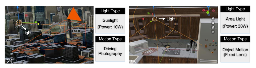
Figure 3: The Car_N (left) and Cook_L (right) in LLR. N (L) means normal (low) light.

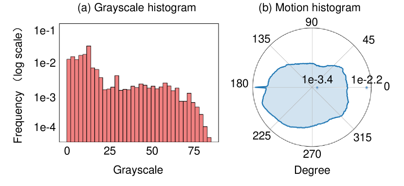
Figure 4: (a) Grayscale histograms of images in low-light scenes, i.e., Ball, Car, Cook, Fan and Rotate with low-light light source. Each bar represents 5 grayscale levels (b) Motion direction histogram of optical flow in LLR.

LLR  As shown in Fig. 2, LLR includes 5$\times$2 carefully designed high-speed scenes where we use the scenes with five kinds of motion (named Ball, Car, Cook, Fan and Rotate) and each scene corresponds to two light sources (normal and low). To ensure the reliability of our scenes, different light sources are used, and the power of light source is consistent with the real world. Specially, we set the lighting parameters in the advanced 3D graphics software, Blender, to make the lighting conditions as consistent as possible with the real world. The following are the configuration details in Blender. In Blender, various types of lighting simulation functions, including sunlight, point lights, and area lights, have been integrated into the graphical interface. We can adjust lighting parameters to control brightness and darkness. For sunlight in Blender, the watts per square meter can be modified. Typically, 100 watts per square meter corresponds to a cloudy lighting environment. For the Car_L scene, as shown in Fig. 3(a), we have set sunlight to 10 watts per square meter, which is deemed sufficiently low. For point lights and area lights, Blender allows modification of radiant Power, measured in watts. This is not the electrical power of consumer light bulbs. A light tube with the electrical power of 30W approximately corresponds to a radiant power of 1W. In the Cook_L scene, as shown in Fig. 3(b), we have set an area light with the radiant Power to 1W (the electrical power of 30W) . It already represents a very dim indoor light source. Each scene in LLR continuously records 21 spike streams with $400\times 250\times 41$ size and 21 corresponding images.

In fact, LLR has diverse grayscale and motion information. To illustrate this fact, we calculate the grayscale distribution and optical flow distribution in LLR. As shown in Fig. 4(a), we can see that the grayscale is diverse and in a lower range. The motion in LLR is also diverse. We generate a optical flow every 40 frames for LLR. The degree distribution of the optical flow is in Fig. 4(b). We can find that the motion in LLR covers all kinds of directions.

4 Method

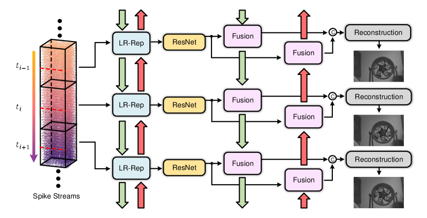
Figure 5: Illustration of the proposed bidirectional recurrent-based reconstruction framework. It includes a light-robust representation, feature extractor (ResNet), fusion and reconstruction. The green and red lines represent the forward and backward data flow. The two kinds of data flow are independent.

4.1 Problem Statement

For simplicity, we write $\mathbf{S}_{t}\in\{0,1\}^{H\times W\times(2\Delta t+1)}$ to denote a spike stream from time $t-\Delta t$ to $t+\Delta t$ ($2\Delta t+1$ is the fixed temporal window) and write $\mathbf{Y}_{t}\in\mathbb{R}^{H\times W}$ to denote the instantaneous light intensity received in spike camera at time $t$. Reconstruction is to use continuous spike streams, $\{\mathbf{S}_{t_{i}},t_{i}=i*(2\Delta t+1)|i=1,2,3...K\}$ to restore the light intensity information at different time, $\{\mathbf{Y}_{t_{i}},t_{i}=i*(2\Delta t+1)|i=1,2,3...K\}$. Generally, the temporal window $2\Delta t+1$ is set as 41 which is the same with [27, 2, 24].

4.2 Overview

To overcome the challenge of low-light spike streams, i.e., the recorded information is sparse (see Fig.1), we propose a light-robust reconstruction method which can fully utilize temporal information of spike streams. It is beneficial from two modules: 1. A light-robust representation, LR-Rep. 2. A fusion module. As shown in Fig. 5, to recover the light intensity information at time $t_{i}$, $\mathbf{Y}_{t_{i}}$, we first calculate the light-robust representation at time $t_{i}$, written as $\mathbf{Rep}_{t_{i}}$. Then, we use a ResNet module to extract deep features, $\mathbf{F}_{t_{i}}$, from $\mathbf{Rep}_{t_{i}}$. $\mathbf{F}_{t_{i}}$ is fused with forward (backward) temporal features as $\mathbf{F}_{t_{i}}^{f}$ ($\mathbf{F}_{t_{i}}^{b}$). Finally, we reconstruct the image at time ${t_{i}}$, $\mathbf{\hat{Y}}_{t_{i}}$ with $\mathbf{F}_{t_{i}}^{f}$ and $\mathbf{F}_{t_{i}}^{b}$.

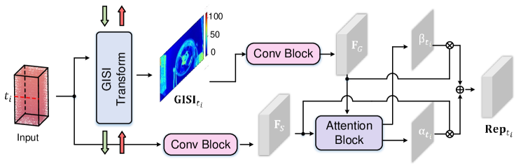
Figure 6: Illustration of the proposed light-robust representation. We use convolution blocks to extract shallow features from input spike stream and GISI, respectively. Then they are fused by an attention block.

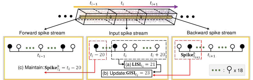
Figure 7: Illustration of GISI transform for backward in a pixel. (a). Calculate the local inter-spike interval, $\mathbf{LISI}_{t_{i}}$ from the input spike stream [2, 29]. (b). Update global inter-spike interval, $\mathbf{GISI}_{t_{i}}$ based on the release time of backward spike, $\mathbf{Spike}_{t_{i+1}}^{b}$ and $\mathbf{LISI}_{t_{i}}$. (c). Maintain and transmit the release time of backward spike, $\mathbf{Spike}_{t_{i}}^{b}$. Black (white) circle is a (no) spike and the red line is backward data flow. More details are shown in algorithm. 1.

4.3 Light-robust Representation

As shown in Fig. 6, a light-robust representation, LR-Rep, is proposed to aggregate the information in low-light spike streams. LR-Rep mainly consists of two parts, GISI transform and feature extraction.

GISI transform  Calculating the local inter-spike interval from the input spike stream is a common operation [2, 29] and we call it as LISI transform. Different from LISI transform, we propose a GISI transform which can utilize the release time of forward and backward spikes to obtain the global inter-spike interval $\mathbf{GISI}_{t_{i}}$. It need to be performed twice, i.e. once forward and once backward respectively. Taking GISI transform for backward as an example, it can be summarized as three steps as shown in Fig. 7. Our GISI transform can extract more temporal information from spike streams than LISI transform as shown in Fig. 8.

Algorithm 1 GISI Transform.

Require:The spike streams at different time {S${}_{t_{i}}$ $|$ i = 1, 2, …, $K$}, $K$ is the number of Continuous spike streams.

1:  Initialize forward state Spike${}_{t_{1}}^{f}$ = 0.

2:  Initialize backward state Spike${}_{t_{K}}^{b}$ = $2K\Delta t$.

3:  for i from 1 to $K$ do

4:     Calculate LISI${}_{t_{i}}$ based on S${}_{t_{i}}$.

5:  end for

6:  for i from 2 to $K$ do

7:     Forward search the recent release time of spike to $t_{i+1}$, Spike${}_{t_{i}}^{f}$ based on S${}_{t_{i}}$.

8:     if Spike${}_{t_{i}}^{f}$ is None then

9:        Set Spike${}_{t_{i}}^{f}$ = Spike${}_{t_{i-1}}^{f}$.

10:     end if

11:     Update GISI${}_{t_{i}}$ based on S${}_{t_{i}}$ and Spike${}_{t_{i-1}}^{f}$.

12:  end for

13:  for i from $K-1$ to 1 do

14:     Backward search the recent release time of spike to $t_{i-1}$, Spike${}_{t_{i}}^{b}$ based on S${}_{t_{i}}$.

15:     if Spike${}_{t_{i}}^{b}$ is None then

16:        Set Spike${}_{t_{i}}^{b}$ = Spike${}_{t_{i+1}}^{b}$.

17:     end if

18:     Update GISI${}_{t_{i}}$ based on S${}_{t_{i}}$ and Spike${}_{t_{i+1}}^{b}$.

19:  end for

20:  Return {GISI${}_{t_{i}}$ $|$ i = 1, 2, …, $K$}

Feature extraction  After GISI transform, we separately extract shallow features of $\mathbf{GISI}_{t_{i}}$ and input spike stream, $\mathbf{F}_{G}$ and $\mathbf{F}_{S}$ through convolution block. Finally, $\mathbf{Rep}_{t_{i}}$ is obtained by an attention module where $\mathbf{F}_{G}$ and $\mathbf{F}_{S}$ are integrated, i.e.,,

$$[\mathbf{\upbeta}_{t_{i}},\mathbf{\upalpha}_{t_{i}}]=Att([\mathbf{F}_{G},\mathbf{F}_{S}]),$$ (3)

$$\mathbf{Rep}_{t_{i}}=\mathbf{\upbeta}_{t_{i}}\mathbf{F}_{G}+\mathbf{\upalpha}_{t_{i}}\mathbf{F}_{S},$$ (4)

where $Att(\cdot)$ denotes an attention block including 3-layer convolution with 3-layer activation function and $\mathbf{Rep}_{t_{i}}$ is our LR-Rep at time ${t_{i}}$. Related details are in our appendix.

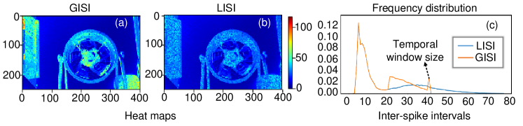
Figure 8: (a) and (b) show the visualizations of $\mathbf{GISI}_{t_{i}}$ and $\mathbf{LISI}_{t_{i}}$ in a real spike stream. (c) shows the distribution of pixel-wise values in $\mathbf{GISI}_{t_{i}}$ and $\mathbf{LISI}_{t_{i}}$.

4.4 Fusion and Reconstruction

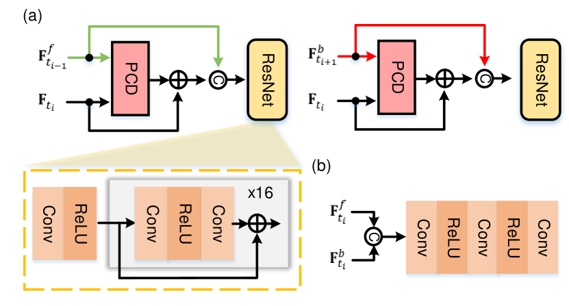
Figure 9: Illustration of fusion module and reconstruction module. (a) denotes forward (green line) and backward (red line) fusion modules. (b) denotes reconstruction module.

We first extract the deep feature $\mathbf{F}_{t_{i}}$ of $\mathbf{Rep}_{t_{i}}$ through a ResNet with 16 layers. Then, as shown in Fig. 9(a), for forward, temporal features $\mathbf{F}_{t_{i-1}}^{f}$ and $\mathbf{F}_{t_{i}}$ are fused as temporal features of the input spike stream $\mathbf{F}_{t_{i}}^{f}$. For backward, temporal features $\mathbf{F}_{t_{i+1}}^{b}$ and $\mathbf{F}_{t_{i}}$ are fused as temporal features of the input spike stream $\mathbf{F}_{t_{i}}^{b}$. To avoid the misalignment of motion from different timestamps, we use a Pyramid Cascading and Deformable convolution (PCD) [19] to add alignment information to $\mathbf{F}_{t_{i}}$. The above process can be written as,

$$\mathbf{F}_{t_{i}}=f(\mathbf{Rep}_{t_{i}}),$$ (5)

$$\mathbf{F}_{t_{i}}^{f}=f([\mathbf{F}_{t_{i}}+a(\mathbf{F}_{t_{i-1}}^{f},\mathbf{F}_{t_{i}}),\mathbf{F}_{t_{i-1}}^{f}]),$$ (6)

$$\mathbf{F}_{t_{i}}^{b}=f([\mathbf{F}_{t_{i}}+a(\mathbf{F}_{t_{i+1}}^{b},\mathbf{F}_{t_{i}}),\mathbf{F}_{t_{i+1}}^{b}]),$$ (7)

where $f(\cdot)$ denotes the feature extraction and $a(\cdot,\cdot)$ denotes the PCD module. Finally, as shown in Fig. 9(b), we use forward and backward temporal features ($\mathbf{F}_{t_{i}}^{b}$ and $\mathbf{F}_{t_{i}}^{f}$) to reconstruct the current scene at time $t_{i}$, i.e.,

$$\mathbf{\hat{Y}}_{t_{i}}=c([\mathbf{F}_{t_{i}}^{b},\mathbf{F}_{t_{i}}^{f}]),$$ (8)

$$\mathcal{L}=\sum\limits_{i=1}^{K}\|\mathbf{\hat{Y}}_{t_{i}}-\mathbf{{Y}}_{t_{i}}\|_{1}$$ (9)

where $c(\cdot)$ denotes 3-layer convolution with 2-layer ReLU, $\mathcal{L}$ is loss function, $\|\cdot\|_{1}$ denotes 1-norm and $K$ is the number of continuous spike streams.

5 Experiment

5.1 Implementation Details

We train our method in the proposed dataset, RLLR. Consistent with previous work [27, 2, 24], the temporal window of each input spike stream is 41. The spatial resolution of input spike streams is randomly cropped the spike stream to $64\times 64$ during the training procedure and the batch size is set as 8. Besides, forward (backward) temporal features and the release time of spikes in our method are maintained from 21 continuous spike streams. We use Adam optimizer with $\beta_{1}=0.9$ and $\beta_{2}=0.99$. The learning rate is initially set as 1e-4 and scaled by 0.1 after 70 epochs. The model is trained for 100 epochs on 1 NVIDIA A100-SXM4-80GB GPU.

5.2 Results

We compare our method with traditional reconstruction methods, i.e., TFI [31], STP [33], SNM [32] and deep learning-based reconstruction methods, i.e., SSML [2], Spk2ImgNet (S2I) [27], WGSE [24]. The supervised learning methods, S2I and WGSE, are retrained on RLLR and the parameter configuration is the same as their respective papers. We evaluate methods on two kinds of data:
(1) The carefully designed synthetic dataset, LLR.
(2) The real spike streams dataset, PKU-Spike-High-Speed [27] and low-light high-speed spike streams dataset [4].

Table 1: PSNR, PSNR_S, and SSIM of reconstruction results on synthetic dataset, LLR. PSNR_S: PSNR is calculated after scaling both the ground truth and reconstructed images to 0-255 (More details are in appendix).

Metric	TFI	SSML	S2I	STP	SNM	WGSE	Ours
PSNR	31.409	38.432	40.883	24.882	25.741	42.959	45.075
PSNRS	21.665	30.176	31.202	14.894	18.527	32.439	38.131
SSIM	0.7231	0.8994	0.9592	0.5554	0.8028	0.97067	0.9868

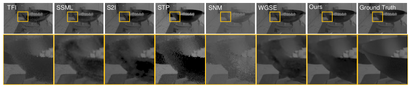
Figure 10: Results from different reconstruction methods on our LLR. More results are in appendix.

Results on our synthetic dataset  As shown in Table. 1, we use the two reference image quality assessment (IQA) metrics, i.e., PSNR, PSNR_S and SSIM to evaluate the performance of different methods on LLR. We can find that our method achieves the best reconstruction performance and has a PSNR gain over 4dB than the reconstruction method, S2I, which demonstrates its effectiveness. Fig. 10 shows the visualization results from different reconstruction methods. We can find that our method can better restore motion details in dark regions than other methods.

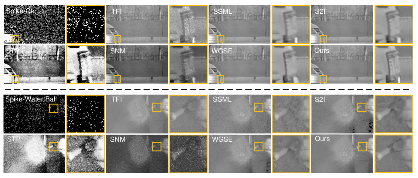
Figure 11: Results from different reconstruction methods on the real datasets, PKU-Spike-High-Speed (Top) and low-light high-speed spike streams dataset (Bottom). More results are in our appendix.

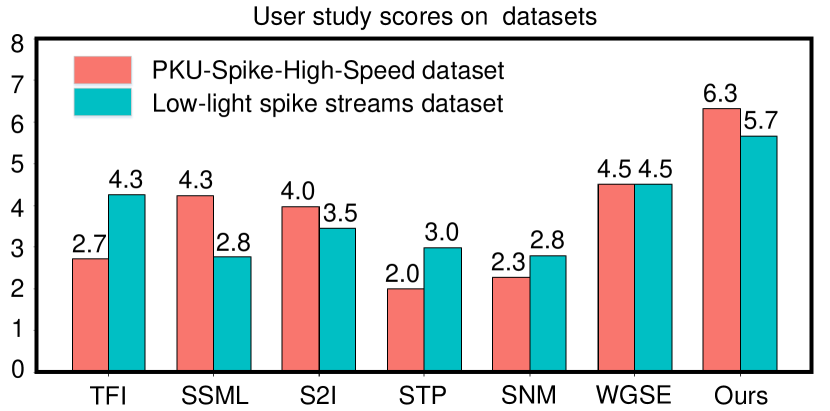
Figure 12: User study scores ($\uparrow$) of reconstructed images from different methods. The max (min) score is 7 (1).

Results on real datasets  For real data, we test different methods on two spike stream datasets, PKU-Spike-High-Speed [27] and low-light spike streams [4]. PKU-Spike-High-Speed includes 4 high-speed scenes under normal-light conditions and [4] includes 5 high-speed scenes under low-light conditions. Fig. 11 shows the reconstruction results. Note that we apply the traditional HDR method [22] to reconstruction results on [4] because scenes are too dark. Our method can more effectively restore the information in scenes i.e., clear texture and less noise.

We perform a user study written as US [21, 9] to quantify the visual quality of different methods. For each scene in datasets, we randomly select reconstructed images at the same time from different methods and display them on the screen (the image order is randomly shuffled). 30 human subjects (university degree or above) are invited to independently score the visual quality of the reconstructed image. The scores of visual quality range from 1 to 7 (worst to best quality). The average subjective scores for each spike stream dataset are shown in Fig. 12 and our method reaches the highest US score in all methods.

Table 2: Comparison between Spk2ImgNet (S2I), WGSE and our method. The input spike stream size is $21\times 41\times 250\times 400$. We test the average of 50 rounds for Inference time.

Method	Para.	Train time	Inference time
S2I	3.91m	2h	1458.45ms
WGSE	3.63m	1h	1344.06ms
Our	5.32m	17h	818.03ms

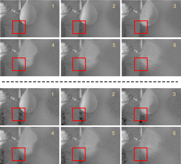
Figure 13: A water polo bursting at high speed in a low-light indoor. We selected the reconstruction results under 6 sampling moments, and the interval between two adjacent sampling moments is 41/40000 s. The above is our method and the bottom is the state-of-the-art reconstruction method [24]. We apply the traditional HDR method [22] to reconstruction results because the scene is too dark.

Stability of continuously reconstructing  Our reconstruction method is stable to spike stream at different moments. Fig. 13 shows the continuous motion of an object in a real high-speed low-light scene. We find that our method can clearly recover motion details at different moments, while the loss introduced by the state-of-the-art WGSE is varied at different time. Besides, we also provide a reconstruction video in our supplementary material.

Network Efficiency Analysis  Table. 2 demonstrates the training time and inference time of the supervised methods, i.e., Spk2ImgNet, WGSE and our method. Although our method requires more training time compared to Spk2ImgNet and WGSE (bidirectional recurrent-based networks typically consume more time during training due to Backpropagation Through Time (BPTT)), our method outperforms Spk2ImgNet and WGSE in terms of inference speed. Besides, due to the need to fuse both forward and backward temporal features, our method is offline, i.e., After spike camera collects spike stream for a long period of time, the data can be reconstructed. In future work, we would extend our method so to online reconstruct.

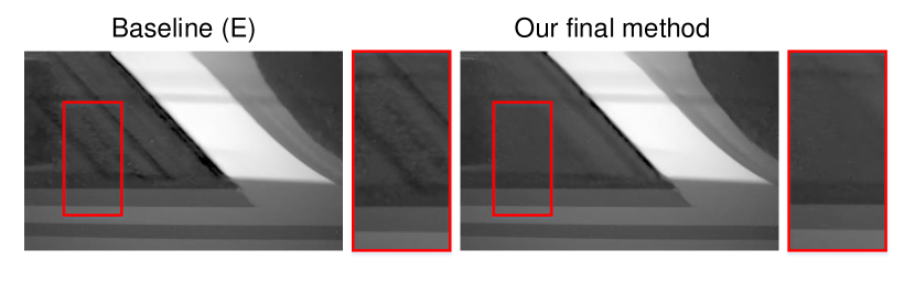
Figure 14: Reconstruction results on a real spike stream. The scene is a high-speed train that exceeds 200 km/h. The glass in the former result (left) shows obvious artifacts, and our result (right) is very smooth and natural.

5.3 Ablation

Proposed modules  To investigate the effect of the proposed light-robust representation LR-Rep, the adjacent (forward and backward) deep temporal features (ADF), i.e., $\mathbf{F}_{t_{i}}^{b}$ and $\mathbf{F}_{t_{i}}^{f}$ in our fusion module, the alignment information in our fusion module (AIF) and GISI transform in LR-Rep, we compare 5 baseline methods with our final method. (A) is the basic baseline without LR-Rep, ADF and AIF. Table. 3 shows ablation results on proposed dataset, LLR. The comparison between (A) and (C) ((B) and (D)) proves the effectiveness of LR-Rep. The comparison between (A) and (B) ((C) and (D)) proves the effectiveness of ADF. Further, by adding the alignment information in the fusion module i.e., AIF, our final method (F) appropriately reduces the misalignment of motion from different timestamps and can reconstruct high-speed scenes more accurately than (D). Besides, the comparison between (E) and (F) shows GISI has better performance than LISI. It is because GISI can extract more temporal information than LISI (see Fig. 8). As shown in Fig. 14, GISI (our final method) not only outperform LISI (Baseline (E) in Table 3) in both PSNR and SSIM on LLR but also have better generalization on real data. More importantly, the cost of using GISI instead of LISI is negligible (we only need to use two 400$\times$250 matrices to store the time of the forward spike and the backward spike, respectively), which does not affect the parameter and efficiency of the network.

Comparison with other representation  We compare the performance of different representation in our framework, i.e., (1) General representation of spike stream: TFI and TFP [31] (2) Tailored representation for reconstruction networks: AMIM [2] in SSML, SALI [27] in S2I and WGSE-1d [24] in WGSE. We replace LR-Rep in our method as above representation. They are retrained on the dataset, RLLR and implementation details are the same with our method. As shown in Table. 4, our LR-Rep achieves the best performance which means LR-Rep can better adapt to our framework.

Table 3: Abltion results on synthetic dataset, LLR.

Index	Effect of different network structures	PSNR	SSIM
(A)	Removing LR-Rep & AIF & ADF	42.743	0.97403
(B)	Removing LR-Rep & AIF	44.151	0.98514
(C)	Removing AIF & ADF	44.739	0.98636
(D)	Removing AIF	44.956	0.98678
(E)	Replace GISI with LISI	44.997	0.98676
(F)	Our final method	45.075	0.98681

Table 4: Performance of different representation methods in our framework. All methods are trained on RLLR and are tested on LLR.

Rep.	TFP	TFI	AMIM	SALI	WGSE-1d	LR-Rep
PSNR	38.615	37.617	41.95	43.314	42.302	45.075
SSIM	0.96641	0.93632	0.97493	0.98304	0.97438	0.98681

The number of continuous spike streams  For solving the reconstruction difficulty caused by inadequate information in low-light scenes, the release time of spike in LR-Rep and temporal features in fusion module are maintained forward and backward in a recurrent manner. The number of continuous spike streams has an impact on our method performance. Fig. 15 shows its effect on the performance. We can find that, as the number increases, the performance of our method can greatly increase until convergence. This is because, as the number increases, our method can utilize more temporal information until sufficient. The reconstrued image from 21 continuous spike streams has more details in a shaded area.

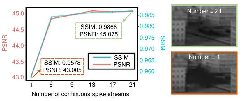
Figure 15: Effect of the number of continuous spike streams on the performance. We test on the dataset, LLR.

Table 5: Reconstruction results on synthetic dataset, LLR. Retrain_idea: our method is retrained on the noise-free version of RLLR.

Metric	Our	Retrainidea
PSNR	45.075	37.679
SSIM	0.98681	0.85374

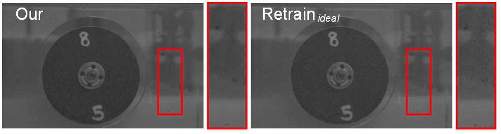
Figure 16: Reconstruction results on a real spike stream. Please enlarge the figure for more details.

Impact of spike camera noise on performance  In proposed datasets, we have considered noise of spike camera refer to [28]. We further discuss the impact of noisy and noise-free spike streams on the performance of our method as shown in Table. 5. We use an ideal spike camera model in SPCS [7] to synthesize a noise-free version of RLLR and retrain our method using the dataset (written as Retrain_idea). We can find that our method has better performance than Retrain_idea. Besides, Fig. 16 shows our method can handle noise in real spike streams better than Retrain_idea.

Table 6: Evaluation results on LLR. We retrain our network where 20%, 40%, 60%, and 80% of RLLR data are used as training set respectively.

Metric	20%	40%	60%	80%	100%
PSNR	35.001	38.618	44.415	44.753	45.075
SSIM	0.93411	0.97113	0.98459	0.98581	0.98681

Train dataset size  The size of train datasets has an impact on the performance of our network. A larger train dataset typically provides more samples and a wider range of variations. In fact, proposed RLLR is enough for the reconstruction task of low-light spike streams. As shown in Table. 6, we find that as the dataset size increase, the performance of the model also improve. However, it is observed that the improvement in performance becomes less significant after the dataset size reaches 60% of RLLR. It shows that the proposed RLLR is sufficient for training our network.

6 Conclusion

We propose a bidirectional recurrent-based reconstruction framework for spike camera to better handle different light conditions. In our framework, a light-robust representation (LR-Rep) is designed to aggregate temporal information in spike streams. Moreover, a fusion module is used to extract temporal features. To evaluate the performance of different methods in low-light high-speed scenes, we synthesize a reconstruction benchmark where light sources are carefully designed to be consistent with reality. The experiment on both synthetic data and real data shows the superiority of our method.

Limitation  Due to the need to fuse both forward and backward temporal features, our method is offline, i.e., After spike camera collects spike streams for a long period of time, the data can be reconstructed. However, real-time applications may require spike stream reconstruction to be performed while the spike camera is capturing the scene. In future work, we plan to extend our method so to online reconstruct.

References

- [1] Christian Brandli, Raphael Berner, Minhao Yang, Shih-Chii Liu, and Tobi Delbruck. A 240 × 180 130 db 3 latency global shutter spatiotemporal vision sensor. IEEE Journal of Solid-State Circuits (JSSC), 49(10):2333–2341, 2014.
- [2] Shiyan chen, Chaoteng Duan, Zhaofei Yu, Ruiqin Xiong, and Tiejun Huang. Self-supervised mutual learning for dynamic scene reconstruction of spiking camera. In Proceedings of the International Joint Conference on Artificial Intelligence, IJCAI, pages 2859–2866, 2022.
- [3] Tobi Delbrück, Bernabe Linares-Barranco, Eugenio Culurciello, and Christoph Posch. Activity-driven, event-based vision sensors. IEEE International Symposium on Circuits and Systems (ISCAS), pages 2426–2429, 2010.
- [4] Yanchen Dong, Jing Zhao, Ruiqin Xiong, and Tiejun Huang. High-speed scene reconstruction from low-light spike streams. In 2022 IEEE International Conference on Visual Communications and Image Processing (VCIP), pages 1–5. IEEE, 2022.
- [5] Rui Graca, Brian McReynolds, and Tobi Delbruck. Optimal biasing and physical limits of dvs event noise. arXiv preprint arXiv:2304.04019, 2023.
- [6] Chunle Guo, Chongyi Li, Jichang Guo, Chen Change Loy, Junhui Hou, Sam Kwong, and Runmin Cong. Zero-reference deep curve estimation for low-light image enhancement. In Proceedings of the IEEE/CVF conference on computer vision and pattern recognition, pages 1780–1789, 2020.
- [7] Liwen Hu, Rui Zhao, Ziluo Ding, Lei Ma, Boxin Shi, Ruiqin Xiong, and Tiejun Huang. Optical flow estimation for spiking camera. In IEEE Conference on Computer Vision and Pattern Recognition (CVPR), pages 17844–17853, 2022.
- [8] Tiejun Huang, Yajing Zheng, Zhaofei Yu, Rui Chen, Yuan Li, Ruiqin Xiong, Lei Ma, Junwei Zhao, Siwei Dong, Lin Zhu, et al. 1000 faster camera and machine vision with ordinary devices. Engineering, 2022.
- [9] Yifan Jiang, Xinyu Gong, Ding Liu, Yu Cheng, Chen Fang, Xiaohui Shen, Jianchao Yang, Pan Zhou, and Zhangyang Wang. Enlightengan: Deep light enhancement without paired supervision. IEEE transactions on image processing, 30:2340–2349, 2021.
- [10] Zhaodong Kang, Jianing Li, Lin Zhu, and Yonghong Tian. Retinomorphic sensing: A novel paradigm for future multimedia computing. In Proceedings of the ACM International Conference on Multimedia (ACMMM), page 144–152, 2021.
- [11] Chongyi Li, Chunle Guo, Linghao Han, Jun Jiang, Ming-Ming Cheng, Jinwei Gu, and Chen Change Loy. Low-light image and video enhancement using deep learning: A survey. IEEE transactions on pattern analysis and machine intelligence, 44(12):9396–9416, 2021.
- [12] Chongyi Li, Chunle Guo, and Chen Change Loy. Learning to enhance low-light image via zero-reference deep curve estimation. IEEE Transactions on Pattern Analysis and Machine Intelligence, 44(8):4225–4238, 2021.
- [13] Chengxi Li, Xiangyu Qu, Abhiram Gnanasambandam, Omar A Elgendy, Jiaju Ma, and Stanley H Chan. Photon-limited object detection using non-local feature matching and knowledge distillation. In Proceedings of the IEEE/CVF International Conference on Computer Vision, pages 3976–3987, 2021.
- [14] Jianing Li, Jiaming Liu, Xiaobao Wei, Jiyuan Zhang, Ming Lu, Lei Ma, Li Du, Tiejun Huang, and Shanghang Zhang. Uncertainty guided depth fusion for spike camera. arXiv preprint arXiv:2208.12653, 2022.
- [15] Patrick Lichtsteiner, Christoph Posch, and Tobi Delbruck. A 128 × 128 120 db 15 latency asynchronous temporal contrast vision sensor. IEEE Journal of Solid-State Circuits (JSSC), 43(2):566–576, 2008.
- [16] Jiaming Liu, Qizhe Zhang, Jianing Li, Ming Lu, Tiejun Huang, and Shanghang Zhang. Unsupervised spike depth estimation via cross-modality cross-domain knowledge transfer. arXiv preprint arXiv:2208.12527, 2022.
- [17] Yukihiro Sasagawa and Hajime Nagahara. Yolo in the dark-domain adaptation method for merging multiple models. In Computer Vision–ECCV 2020: 16th European Conference, Glasgow, UK, August 23–28, 2020, Proceedings, Part XXI 16, pages 345–359. Springer, 2020.
- [18] Jing Wang, Peng Yang, Yuansheng Liu, Duo Shang, Xin Hui, Jinhong Song, and Xuehui Chen. Research on improved yolov5 for low-light environment object detection. Electronics, 12(14):3089, 2023.
- [19] Xintao Wang, Kelvin C.K. Chan, Ke Yu, Chao Dong, and Chen Change Loy. Edvr: Video restoration with enhanced deformable convolutional networks. In Proceedings of the IEEE/CVF Conference on Computer Vision and Pattern Recognition (CVPR) Workshops, June 2019.
- [20] Chen Wei, Wenjing Wang, Wenhan Yang, and Jiaying Liu. Deep retinex decomposition for low-light enhancement. arXiv preprint arXiv:1808.04560, 2018.
- [21] Tom D Wilson. On user studies and information needs. Journal of documentation, 37(1):3–15, 1981.
- [22] Zhenqiang Ying, Ge Li, and Wen Gao. A bio-inspired multi-exposure fusion framework for low-light image enhancement. arXiv preprint arXiv:1711.00591, 2017.
- [23] Mingliang Zhai, Kang Ni, Jiucheng Xie, and Hao Gao. Spike-based optical flow estimation via contrastive learning. In ICASSP 2023-2023 IEEE International Conference on Acoustics, Speech and Signal Processing (ICASSP), pages 1–5. IEEE, 2023.
- [24] Jiyuan Zhang, Shanshan Jia, Zhaofei Yu, and Tiejun Huang. Learning temporal-ordered representation for spike streams based on discrete wavelet transforms. In Proceedings of the AAAI Conference on Artificial Intelligence, volume 37, pages 137–147, 2023.
- [25] Jiyuan Zhang, Lulu Tang, Zhaofei Yu, Jiwen Lu, and Tiejun Huang. Spike transformer: Monocular depth estimation for spiking camera. In European Conference on Computer Vision (ECCV), 2022.
- [26] Jing Zhao, Ruiqin Xiong, and Tiejun Huang. High-speed motion scene reconstruction for spike camera via motion aligned filtering. In International Symposium on Circuits and Systems (ISCAS), pages 1–5, 2020.
- [27] Jing Zhao, Ruiqin Xiong, Hangfan Liu, Jian Zhang, and Tiejun Huang. Spk2imgnet: Learning to reconstruct dynamic scene from continuous spike stream. In IEEE Conference on Computer Vision and Pattern Recognition (CVPR), pages 11996–12005, 2021.
- [28] Junwei Zhao, Shiliang Zhang, Lei Ma, Zhaofei Yu, and Tiejun Huang. Spikingsim: A bio-inspired spiking simulator. In 2022 IEEE International Symposium on Circuits and Systems (ISCAS), pages 3003–3007. IEEE, 2022.
- [29] Rui Zhao, Ruiqin Xiong, Jing Zhao, Zhaofei Yu, Xiaopeng Fan, and Tiejun Huang. Learninng optical flow from continuous spike streams. In Proceedings of the Annual Conference on Neural Information Processing Systems (NeurIPS), 2022.
- [30] Yajing Zheng, Lingxiao Zheng, Zhaofei Yu, Boxin Shi, Yonghong Tian, and Tiejun Huang. High-speed image reconstruction through short-term plasticity for spiking cameras. In IEEE Conference on Computer Vision and Pattern Recognition (CVPR), pages 6358–6367, 2021.
- [31] Lin Zhu, Siwei Dong, Tiejun Huang, and Yonghong Tian. A retina-inspired sampling method for visual texture reconstruction. In IEEE International Conference on Multimedia and Expo (ICME), pages 1432–1437, 2019.
- [32] Lin Zhu, Siwei Dong, Jianing Li, Tiejun Huang, and Yonghong Tian. Ultra-high temporal resolution visual reconstruction from a fovea-like spike camera via spiking neuron model. IEEE Transactions on Pattern Analysis and Machine Intelligence, 45(1):1233–1249, 2022.
- [33] Lin Zhu, Jianing Li, Xiao Wang, Tiejun Huang, and Yonghong Tian. Neuspike-net: High speed video reconstruction via bio-inspired neuromorphic cameras. In IEEE International Conference on Computer Vision (ICCV), pages 2400–2409, 2021.